Sticky prices and comovement of business cycle

Sticky prices and comovement of business cycle∗

Junhee Lee†‡

Abstract

A defining characteristic of business cycle is comovements of economicvariables across sectors. But it is not easy to replicate these comovementsin standard real business cycle models. Traditionally, however, not onlythe productivity shocks emphasized in real business cycle models but alsomonetary shocks have been believed to be important in explaining businesscycles. Following this tradition, a two sector sticky price model is con-structed in this paper to examine the sectoral comovements of economicvariables under nominal rigidities. It turns out that monetary shocks cangenerate comovements of sectoral variables.

Keywords: Comovement over business cycles, Sticky prices, Stickywages

JEL Classification: F32

∗I’d like to thank professor Paul Evans for his guidance and valuable advices. Also I’dlike to thank macro lunch participants at the Ohio State University. All remaining errors aremine.

†Department of Economics, The Ohio State University, 321 Arps Hall, 1945 N. High Street,Columbus, OH 43210.

‡E-mail address : [email protected]

1

1 IntroductionAs noted in Huffman and Wynne (1998), a defining characteristic of businesscycles, whether in the traditional sense of Burns and Mitchell (1946) or in thecontemporary sense of Lucas (1977), is the comovement in the pace of economicactivity in different sectors of the economy. Also according to Christiano andFitzgerald (1998) and Huffman and Wynne (1998), levels of output, employmentand investment in various sectors of the economy move in a procyclical manneralthough they do not move perfectly in tandem.As an example, Huffman and Wynne (1998) divided the U.S. economy into

consumption and investment sectors, and they report the correlations of output,capital, labor input and investment flow in consumption sector and investmentsector with aggregate output as shown in table1. Using the 1987 input-outputtables to determine how much of a sector’s final output goes to consumption asopposed to investment or intermediate uses, they classified a sector as belongingto the consumption sector if the bulk of the sector’s final output is allocated tofinal consumption demand and a sector as belonging to the investment sectorotherwise. Using this criterion, they classified the finance, insurance and realestate(FIRE), retail trade and services sectors as the consumption sector andthe mining, construction, manufacturing, transportation and public utilities andwholesale trade sectors as the investment sector. Table1 shows that the outputsin both sectors are procyclical and the output of the investment sector is morecorrelated with aggregate output than output of the consumption sector, andis also nearly three times more volatile. The labor inputs in both sectors arealso strongly procyclical, and the labor input in the investment sector is nearlytwice as volatile as the labor input in the consumption sector. Finally sectoralinvestment flows show procyclical movements. Huffman and Wynne (1998) alsoreports that more detailed sectoral data show similar patterns.However, it is not easy to replicate the sectoral comovement of economic

variables in a business cycle model. In standard real business cycle models, asshown in Christiano and Fitzgerald (1998), a positive productivity shock in-duces labor hours and investment in the consumption sector to move negativelynot positively, in contrast with data.1 Christiano and Fitzgerald (1998) docu-ments various approaches to solve this "comovement puzzle" in the real businesscycle models. Such approaches include Benhabib et al. (1991) which incorpo-rates household production as a third sector, Hornstein and Praschnik (1997)which stresses intermediate input channel, Huffman and Wynne (1998) whichintroduces intratemporal adjustment costs in producing investment goods, andChristiano and Fisher (1998) which modifies standard model by introducing la-bor immobility and habit persistence. But also limitations of these approaches

1Christiano and Fitzgerald (1998) explains as follows. When a positive productivity shockhits the economy, the outputs of both consumption and investment goods sector increase.However, there is a relatively larger increase in the output of investment goods reflecting therise of opportunity cost of applying resources to the consumption sector and the consumptionsmoothing motives of households. The increase in the demand for investment goods relative toconsumption goods implies that capital and labor resources are shifted out of the productionof consumption goods and into the production of investment goods.

2

are documented in Christiano and Fitzgerald (1998) and possible new lines ofapproaches to solve this "puzzle" such as incorporating strategic complementar-ity, information externalities, and efficiency wages are suggested in Christianoand Fitzgerald (1998).On the other hand, economists have explained business cycle phenomena not

only in terms of productivity shocks emphasized in real business cycle models,but also in terms of aggregate demand shocks. And traditionally monetaryshocks have been believed to be important sources of business cycle fluctuationsas in Friedman and Schwartz (1963). Along this line of thought, we can findsticky price and wage models such as Chari et al. (2000), Christiano et al.(2001) and Erceg et al. (2000) which try to explain fluctuations of economicvariables in terms of monetary shocks. Thus it is very natural to examine thebehavior of a sticky price and wage model in a two sector setting so that wecan see whether monetary shocks can explain sectoral movements(particularlycomovement) better than productivity shocks. Since monetary shocks, whichare demand shocks by nature, can work differently from productivity shocks,which are supply shocks by nature, they may explain the sectoral comovementof business cycles better than productivity shocks. Simply put, when a monetaryshock hits the economy, this can increase demand across all sectors, leading tothe possible comovement of economic variables across the sectors.But until now, there has been virtually no attempt to explain the comove-

ment of sectoral variable in terms of aggregate demand shocks or more specifi-cally monetary shocks. So in this paper, we construct a two sector sticky priceand wage model to see whether monetary shocks can generate a realistic co-movement of economic variables in the model economy.The main findings from this attempt can be summarized as follows. First

monetary shocks can generate comovement of sectoral variables in the modeleconomy and volatility and correlation statistics in the model economy are sim-ilar to the actual data. And this result is obtained by a fairly standard two sectorsticky price and wage model constructed below and thus we can say monetaryshocks naturally and inherently generate the comovement of economic variablesin sticky price and wage model without any major modifications. Second, pro-ductivity shocks do not generate comovement of economic variables in the modelconstructed below. We observe negative responses of aggregate inputs after apositive productivity shock due to the stickiness in price and wage as explainedin Gali (2000). In addition, we observe that labor input in each sector movesin the opposite direction when there is a productivity shock in the investmentsector, as can be seen in standard two sector real business cycle models.Thus we can explain the comovement of economic variables very easily with

monetary shocks in a sticky price and wage model. But we can not easilygenerate the comovement with productivity shocks in the model and at leastsome modifications, like those tried in real business cycle models, are needed toobtain the comovement when productivity shocks are used as sources of businesscycles.The rest of the paper is organized as follows. In section 2, we describe the

model. In section 3, we characterize the equilibrium of the model and calibrate

3

parameters. In section 4, we summarize findings from our benchmark modeland its variations. And in section 5, we conclude.

2 Model Economy

2.1 General Description

The model basically modifies Chari et al. (2000) which is one sector stickyprice model and also incorporates several other minor modifications. In eachperiod t, the model economy experiences an event st in St which is a set of allpossible events at t.We denote by st = (s0, ..., st) the history of events up through and including

period t. The probability as of period 0, of any particular history st is π(st).The initial realization s0 is given.There are two sectors in this economy. One sector produces a consumption

good and the other sector produces a durable investment good. This followsfrom standard two sector models such as Huffman and Wynne (1998) and Chris-tiano and Fisher (1998). The consumption good is produced by aggregating acontinuum of intermediate goods and is sold to the market competitively. In-termediate goods for the production of consumption good are produced usinglabor and capital and sold by imperfect competitors. And intermediate goodsproducers set prices in a staggered fashion as in Taylor (1980).The investment sector works similar to the consumption sector except that

there is an intratemporal adjustment costs in producing investment goods as inHuffman and Wynne (1998) which will be explained below.In the labor market, wages are also determined in a staggered fashion.

Namely we introduce sticky wages by letting labor be differentiated and in-troducing monopolistically competitive unions that set wages in a staggeredway as in Chari et al. (2002). We also introduce intratemporal adjustmentcosts in the labor supply as in investment good production.

2.2 Agents’ Problems

2.2.1 Consumption Good Sector

Final consumption good is produced by applying following technology:

yc(st) =

·Zydc (i, s

t)θcdi

¸ 1θc

(1)

where yc(st) is the consumption good, ydc (i, st) is an intermediate good of type

i ∈ [0, 1] used for the production of consumption good. And the elasticity ofsubstitution between the intermediate goods is 1/(1− θc).

4

The technology for producing each intermediate good i is a standard Cobb-Douglas production function given as

yc(i, st) = kdc (i, s

t)α1(λc(st)ldc (i, s

t))1−α1 (2)

where kdc (i, st) and ldc (i, s

t) are the capital and labor inputs used to producethe ith intermediate good. And λc(st) is consumption sector productivity shockrepresented in labor augmenting form as in Huffman and Wynne (1998). Alsoα1 is the parameter for the Cobb-Douglas production function.Final consumption good producers behave competitively and in each period

t, they choose intermediate inputs ydc (i, st) for all i ∈ [0, 1], and output yc(st)

to maximize the profits given as

maxP c(st)yc

¡st¢− Z Pc(i, s

t−1)ydc (i, st)di (3)

subject to (1), where P c(st) is the price of the final consumption good in period

t and Pc(i, st−1) is the price of intermediate good i used for the consumption

good production in period t. We assume period t intermediate goods pricesare set before the realization of the period t shocks, thus intermediate goodsprices do not depend on st. Solving the problem in (3) gives the input demandfunctions:

ydc (i, st) =

·P c (s

t)

Pc(i, st−1)

¸ 1(1−θc)

yc(st) (4)

The zero-profit condition implies that

P c(st) =

·ZPc(i, s

t−1)θc

θc−1

¸ θc−1θc

(5)

In equilibrium the consumption good price in period t depends only on st−1 dueto the price setting assumption of the intermediate goods producers.Intermediate goods producers behave as imperfect competitors. They set

prices for N periods and do so in a staggered fashion. In particular, in eachperiod t, a fraction 1/N of these producers choose new prices Pc(i, st−1) be-fore the realization of the event st. These prices are set for N periods, sofor this group of intermediate goods producers, Pc(i, st+τ−1) = Pc(i, s

t−1) forτ = 0, ..., N − 1. The intermediate goods producers are indexed so that produc-ers indexed i ∈ [0, 1N ] set new prices in 0, N, 2N, and so on, while producersindexed i ∈ [ 1N , 2N ] set new prices in 1, N + 1, 2N + 1, and so on, for the Ncohorts of intermediate goods producers. Intermediate goods producers whoseprice setting constraint is Pc(i, st+τ−1) = Pc(i, s

t−1) for τ = 0, ..., N − 1, maxi-mize discounted profits from period t to period t+N − 1 given as:

maxPc(i,st−1),kdc (i,sτ ),ldc(i,sτ )

t+N−1Xτ=t

Xsτ

Q(sτ¯̄st−1

¢[Pc(i, s

t−1)yc(i, sτ )

5

−P c(sτ )rc(s

τ )kdc (i, sτ )− P c(s

τ )wc(sτ )ldc (i, s

τ )] (6)

subject to (2), (4), where Q(sτ¯̄st−1

¢is the price of one dollar in sτ in units of

dollars at st−1, rc(sτ ) is the rental rate on capital and wc(sτ ) is the real wage

rate evaluated in terms of final consumption good.First order conditions imply2

Pc(i, st−1) =

Pt+N−1τ=t

Psτ Q(s

τ¯̄st−1

¢P c(s

τ )(2−θc)/(1−θc)υc(sτ )yc(sτ )

θcPt+N−1

τ=t

Psτ Q(s

τ |st−1)P c(sτ )1/(1−θc)yc(sτ )(7)

where υc(sτ ) is given as

υc(sτ ) =

1

(1− α1)λc(sτ )wc(s

τ )

µλc(s

τ )ldc (i, sτ )

kdc (i, sτ )

¶α1(8)

And also from the first order conditions, we getµ1− α1α1

¶kdc (i, s

t)

ldc (i, st)=

wc(st)

rc (st)(9)

Given the constant elasticity of substitution (CES) property of Cobb-Douglasfunction, this implies that capital-labor ratios are equated across the interme-diate goods firms, so for all i ∈ [0, 1],

kdc (i, st)

ldc (i, st)=

kdc (0, st)

ldc (0, st)

(10)

2.2.2 Investment Good Sector

Durable investment goods are produced in the investment sector for the use ofconsumption sector and for its own use. The basic structure of the investmentsector is similar to the consumption sector. But we will introduce intratemporaladjustment costs discussed in Huffman and Wynne (1998).3

Producers who produce investment goods for both sectors produce the re-quired investment goods using a composite investment good yi(s

t). And thecomposite investment good yi(s

t) is produced in turn by aggregating its inter-mediate goods.Production technology for the composite good yi(s

t) is given as follows,which is analogous to the final consumption good in the consumption sector.

yi(st) =

·Zydi (j, s

t)θidj

¸ 1θi

(11)

2Appendix containing detailed derivaitons is available upon request.3Huffman and Wynne (1998) generates sectoral comovement of investment by incorporating

this type of intratemporal adjustment costs in a two sector real business cycle model.

6

where ydi (j, st) is intermediate good of type j ∈ [0, 1] used for the produc-

tion of yi(st). The elasticity of substitution between the intermediate goods is1/ (1− θi).And the technology for the production of intermediate good yi(j, st) is given

asyi(j, s

t) = kdi (j, st)α2(λi(s

t)ldi (j, st))1−α2 (12)

where kdi (j, st) and ldi (j, s

t) are the capital and labor inputs used to producejth intermediate good. λi(s

t) is productivity shock in the investment sector,and α2 is a parameter.The production of investment goods is then allocated across the two sectors

according to the relationship:

Υ[φic(st)−ρ + (1− φ)ii(s

t)−ρ]−1/ρ = ydi (st) (13)

where ic(st) is the investment good produced for consumption sector, and ii(st)is the investment good produced for investment sector. ydi (s

t) is the compos-ite good used for the production of investment goods. And φ, ρ and Υ areparameters.We need some explanations concerning (13). With φ = 0.5, ρ = −1 and

Υ = 2, (13) becomes standard resource constraint for the investment goods.That is, total investment(yi(st)) is the sum of investment good produced forthe consumption good sector and investment good sector. However, changingthese parameters we can change the relative price of the two investment goods.Figure1 illustrates some relevant facts where we change parameter ρ settingφ = 0.5 and Υ = 2. For the standard case when ρ = −1, there is an infiniteelasticity of substitution between ic(s

t) and ii(st). This means that it is very

easy to switch from the production of one type of investment good into that ofanother. Specifically, by cutting back the production of new investment goodfor one sector by one unit, it is possible to increase production of new invest-ment good for the other sector by one unit without incurring further costs. It isplausible that an economy can alter its capacity for producing heavy equipmentfor industrial use on the one hand, and alternative equipment for services sectoruse on the other. However, in practice it can be costly to do so quickly. Now, asthe absolute value of ρ gets bigger, it becomes more difficult to alter the com-position of investment goods produced. The motivation of this specification isthat it takes time and resources to change the composition of investment goodsproduced. This is referred to as intratemporal adjustment costs in Huffmanand Wynne (1998), since we encounter decreasing marginal returns in produc-ing more of one type of investment good while reducing the production of thealternative investment good at a particular moment in time.Investment goods producers act competitively and their problem is specified

as follows:maxPicic(s

t) + Piiii(st)− P iy

di (s

t) (14)

subject to (13), where Pic, Pii, and P i are prices for ic(st), ii(st), and ydi (st)

7

respectively. The first order conditions for investment goods producers are:

Pic(st)

P i(st)= Υ[φic(s

t)−ρ + (1− φ)ii(st)−ρ]−(1+ρ)/ρφic(st)−ρ−1 (15)

Pii(st)

P i(st)= Υ[φic(s

t)−ρ + (1− φ)ii(st)−ρ]−(1+ρ)/ρ(1− φ)ii(s

t)−ρ−1 (16)

The composite good producers behave competitively and in each period t,they choose inputs yi (j, st) for all j ∈ [0, 1], and output yi(st) to maximizeprofits:

maxP i(st)yi

¡st¢− Z Pi(j, s

t−1)ydi (j, st)dj (17)

subject to (11). Solving the problem in (17) gives the input demand functions:

ydi (j, st) =

·P i(s

t)

Pi(j, st−1)

¸ 1

(1−θi)yi(s

t) (18)

The zero-profit condition implies that

P i(st) =

·ZPi(j, s

t−1)θi

θi−1

¸ θi−1θi

(19)

The intermediate goods producers in this sector work analogous to those inthe consumption sector. Namely, they set prices for M periods and do so ina staggered fashion. In particular, in each period t, a fraction 1/M of theseproducers choose new prices Pi(j, st−1) before the realization of the event st.These prices are set for M periods, so for this group of intermediate goodsproducers, Pi(j, st+τ−1) = Pi(j, s

t−1) for τ = 0, ...,M − 1. The intermediategoods producers are indexed so that producers indexed j ∈ [0, 1M ] set newprices in 0, M, 2M, and so on, while producers indexed j ∈ [ 1M , 2M ] set newprices in 1, M + 1, 2M + 1, and so on, for the M cohorts of intermediategoods producers. Intermediate goods producers whose price setting constraintis Pi(j, st+τ−1) = Pi(j, s

t−1) for τ = 0, ...,M − 1, maximize discounted profitsfrom period t, to period t+M − 1. That is, each solves problem:

maxPi(j,st−1),kdi (j,sτ ),l

di (j,s

τ )

t+M−1Xτ=t

Xsτ

Q(sτ¯̄st−1

¢[Pi(j, s

τ−1)yi(j, sτ )

−P i(sτ )ri(s

τ )kdi (j, sτ )− P i(s

τ )wi(sτ )ldi (j, s

τ )] (20)

subject to (12), (18), where ri(sτ ), wi(sτ ) are rental rate of capital and wage

rate in the investment sector evaluated in terms of investment composite good,The first order conditions imply

Pi(j, st−1) =

Pt+M−1τ=t

Psτ Q(s

τ¯̄st−1

¢P i(s

τ )(2−θi)/(1−θi)υi(sτ )yi(sτ )

θiPt+M−1

τ=t

Psτ Q(s

τ |st−1)P i(sτ )1/(1−θi)yi(sτ )(21)

8

where υi(sτ ) is given as

υi(sτ ) =

1

(1− α2)λi (sτ )wi(s

τ )

µλi (s

τ ) ldi (j, sτ )

kdi (j, sτ )

¶α2(22)

And also from the first order conditionsµ1− α2α2

¶kdi (j, s

t)

ldi (j, st)=

wi(st)

ri (st)(23)

Given the CES property of Cobb-Douglas function, this implies that capital-labor ratios are equated across the intermediate goods firms, so for all j ∈ [0, 1],

kdi (j, st)

ldi (j, st)=

kdi (0, st)

ldi (0, st)

(24)

2.2.3 Labor and Capital Supplying Firms

We introduce labor and capital supplying firms for ease of analysis. Laborsupplying firms will supply labor to both sectors in the presence of intratemporaladjustment costs analogous to the investment goods production. Namely, laborsupplying firms will provide labor for both sectors using composite labor l (st)and the constraint for the labor supply is given as:

Φ[ lc(st)−κ + (1− )li(s

t)−κ ]−1/κ = ld(st) (25)

where lc(st) is the labor supply for consumption sector, and li(s

t) is the la-bor supply for investment sector. ld(st) is the composite labor used for theprovision of labor for each sector. And Φ, and κ are parameters. We intro-duce intratemporal adjustment costs in labor supply because it is also costly toreallocate labor between sectors quickly.Labor supplying firms act competitively and their problem is specified as

follows:

maxP c(st)wc(s

t)lc(st) + P i(s

t)wi(st)li(s

t)−W¡st¢ld(st) (26)

subject to (25), where W is price for labor l(st). The first order conditions forlabor supplying firms imply

P c(st)wc(s

t)

W (st)= Φ[ lc(s

t)−κ + (1− )li(st)−κ ]−(1+κ )/κ lc(s

t)−κ−1 (27)

P i(st)wi(s

t)

W (st)= Φ[ lc(s

t)−κ +(1− )li(st)−κ ]−(1+κ )/κ (1− )li(s

t)−κ−1 (28)

9

Composite labor is created by aggregating a continuum of differentiated laborinputs l (q, st) , provided by labor unions of type q ∈ [0, 1]. That is,

l¡st¢=

·Zld¡q, st

¢ϑdq

¸1/ϑ(29)

where l (st) is composite labor, ld (q, st) is the amount of differentiated laborinput of type q, and ϑ is a parameter. And the composite labor is providedcompetitively. Thus each composite labor providing firm solves following prob-lem

maxW¡st¢l(st)−W

¡q, st−1

¢ld(q, st) (30)

subject to (29). The first order conditions to this problem imply,

ld(q, st) =

µW (st)

W (q, st−1)

¶ 11−ϑ

l¡st¢

(31)

where W (st) =hR

W (q, st−1)ϑ

ϑ−1 dqiϑ−1

ϑ

.

Now let’s turn to the capital supplying firms. Capital used for the consump-tion sector is provided by competitive capital leasing firms (below referred as theconsumption sector capital leasing firm) which maximize the following problem

∞Xτ=t

Xsτ

Q(sτ¯̄st¢ {P c(s

τ )rc (sτ ) kc(s

τ−1)− Pic (sτ ) idc (s

τ )} (32)

subject to the law of motion for capital accumulation.4

kc(st) = (1− δ1)kc(s

t−1)− bc2

µic (s

t)

kc (st−1)− δ1

¶2kc¡st−1

¢+ ic

¡st¢

(33)

Here, δ1 denotes the depreciation rate of capital.The first order conditions are5

Pic¡st¢= ξ

¡st¢½1− bc

µic (s

t)

kc (st−1)− δ1

¶¾(34)

ξ¡st¢=Xst+1

Q(st+1¯̄st¢ £P c(s

t+1)rc¡st+1

¢+ ξ

¡st+1

¢ {(1− δ1)

−bc2

Ãic¡st+1

¢kc (st)

− δ1

!2+ bc

Ãic¡st+1

¢kc (st)

− δ1

!ic¡st+1

¢kc (st)

(35)

4This form of capital accumulation equation is from Chari et al. (2000). Also capital isimmobile across sectors and thus we have a separate capital accumulation equation in eachsector as in Huffman and Wynne (1998).

5Appendix containing detailed derivaitons is available upon request.

10

where ξ (st) is Lagrangian multiplier associated with the law of motion for cap-ital accumulation.The capital used for the investment sector is provided similarly. Thus com-

petitive capital leasing firms (below referred as the investment sector capitalleasing firm) maximize the following objective function.

∞Xτ=t

Xsτ

Q(sτ¯̄st¢ {P i(s

τ )ri (sτ ) ki(s

τ−1)− Pii (sτ ) idi (s

τ )} (36)

subject to the law of motion for capital accumulation

ki(st) = (1− δ2)ki(s

t−1)− bi2

µii (s

t)

ki (st−1)− δ2

¶2ki¡st−1

¢+ ii

¡st¢

(37)

Here, δ2 denotes the depreciation rate of capitalFirst order conditions imply

Pii¡st¢= κ

¡st¢½1− bi

µii (s

t)

ki (st−1)− δ2

¶¾} (38)

κ¡st¢=Xst+1

Q(st+1¯̄st¢ £P i(s

t+1)ri¡st+1

¢+ κ

¡st+1

¢ {(1− δ2)

−bi2

Ãii¡st+1

¢ki (st)

− δ2

!2+ bi

Ãii¡st+1

¢ki (st)

− δ2

!ii¡st+1

¢ki (st)

(39)

where κ(st) is Lagrangian multiplier associated with the law of motion for capitalaccumulation.

2.2.4 Consumer Problem

The consumer side of the market is organized into a continuum of unions indexedby q ∈ [0, 1]. Union q consists of all the consumers in the economy with type qlabor. Each union realizes that it faces a downward-sloping demand for its owntype of labor. Namely, the total demand for type q labor is given as (31). Weassume that a fraction 1/G of unions set their wages in a given period and holdwages fixed for G subsequent periods. The unions are indexed so that thosewith q ∈ [0, 1/G] set new wages in 0, G, 2G, and so on, while those withq ∈ [1/G, 2/G] set new wages in 1, G+1, 2G+1, and so on, for the G cohortsof unions. In each period, these new wages are set before the realization of theevent st. Notice that the wage-setting arrangement is analogous to the price-setting arrangement for intermediate goods producers in both consumption andinvestment sector.

11

Total discounted expected utility for the qth union is given as

∞Xt=0

Xst

βtπ¡st¢U(c(q, st), l(q, st),M(q, st)/P c(s

t)) (40)

where 0 < β < 1 is the discount factor and c(q, st), l(q, st), andM(q, st)/P c(st)

are consumption in period t , labor in period t, and real balances in period trespectively.Temporal utility function is given as

U(c(q, st), l(q, st),M(q, st)/P c(st))

=c(q, st)1−σ

1− σ+ ψ

(1− l (q, st))1−γ

1− γ+ ω

¡M(q, st)/P c(s

t)¢1−η

1− η(41)

where ω and ψ are relative weight parameters, η is interest elasticity of realbalance, σ is risk aversion, and γ is labor elasticity.The budget constraints are given as

P c(st)c(q, st) +M(q, st) +

Xst+1

Q(st+1¯̄st¢B(q, st+1)

≤W (q, st−1)l(q, st) +M(q, st−1) +B(q, st) +Π¡st¢+ T (st) (42)

where Π (st) is the nominal profits of the intermediate goods producers, andT (st) is nominal transfers. Each of the nominal bonds B(q, st+1) is a claim toone dollar in state st+1 and costs Q(st+1 |st) dollars in state st. In terms ofrelating the prices in the intermediate goods producers’ problem to these prices,note that Q(sτ |st) = Q(st+1 |st)Q(st+2 ¯̄st+1¢ · ·· Q(sτ ¯̄sτ−1¢ for all τ > t.The problem of the qth union is thus to maximize (40) subject to the la-

bor demand schedule (31), the budget constraints (42), and the wage settingconstraints W (q, st+τ−1) = W (q, st−1) for τ = 0, ...,M − 1. The first orderconditions are6

ζ¡q, st

¢=

U1 (q, st)

P c (st)(43)

W (q, st−1) = −Pt+G−1

τ=t

Psτ β

τ−t+1π(st+1 |st)W (sτ )1

1−ϑ l(sτ )U2(q, sτ )

ϑPt+G−1

τ=t

Psτ β

τ−t+1π(st+1 |st) ζ (q, sτ )W (sτ )1

1−ϑ l(sτ )(44)

U3(q, st)

P c(st)− ζ

¡q, st

¢+ β

Xst+1

π(st+1¯̄st¢ζ¡q, st+1

¢= 0 (45)

Q(sτ¯̄st¢= βτ−tπ(sτ

¯̄st¢ ζ ¡q, st+1¢

ζ (q, st)(46)

for all τ > t, where ζ (q, st) is Lagrangian multiplier associated with budgetconstraint in period t, U1(st), U2(st), and U3(s

t) denote the derivatives of the

6Appendix containing detailed derivaitons is available upon request.

12

utility function with respect to its arguments and π(sτ |st) = π(sτ )/π(st) is theconditional probability of sτ given st . Notice that (46) imply that

ζ¡q, st+1

¢ζ (q, st)

=ζ¡q0, st+1

¢ζ (q0, st)

(47)

for all q, and q0. So, Lagrangian multipliers of different type of union are equatedup to a factor of proportionality, namely the date 0 Lagrangian multiplier ontheir budget constraint. Here, we assume that initial debts and transfers amongthe G types in the economy are such that the multipliers are equated. In thatcase, we have

U1¡q, st

¢= U1

¡q0, st

¢(48)

U3¡q, st

¢= U3

¡q0, st

¢(49)

for all q, and q0 from (43) and (45).

2.2.5 Money Supply

The nominal money supply process is given by

M(st) = µ¡st¢M¡st−1

¢(50)

where µ (st) follows a first order autoregressive process

logµ¡st¢= ρµ logµ

¡st−1

¢+ µ(s

t) (51)

where µ(st) is independent and identically normally distributed mean zero

shock with standard deviation σ µ . New money balances are distributed to con-sumers in a lump sum fashion by having nominal transfers satisfying T (st) =M (st)−M

¡st−1

¢.

2.2.6 Productivity Shock

Productivity shocks λc(st) and λi(st) jointly obey the following law of motion:

Λt ≡·log(λc(s

t))log (λi(s

t))

¸= ΓΛt−1 + λ(s

t) (52)

where Γ is autoregressive matrix and λ(st) is independent, identically and

normally distributed mean zero shock with covariance matrix Σλwhich is sym-

metric positive definite.

13

2.3 Market Equilibrium

In terms of market-clearing conditions, consider first the factor markets. Thecapital supply for the consumption sector is kc(st−1).7 On the demand side, weneed to aggregate demand for capital by each intermediate goods producer i inconsumption sector kdc (i, s

t) , i ∈ [0, 1]. Analogous reasoning also holds for capi-tal market for investment sector. Thus market clearing conditions for the capitalused for the consumption sector and the investment sector are respectively,

kc(st−1) =

Zkdc (i, s

t)di ≡ kdc (st) (53)

ki(st−1) =

Zkdi (j, s

t)dj ≡ kdi (st) (54)

We denote aggregate demands for capital in consumption and investment sectoras kdc (s

t) and kdi (st) respectively.

Similarly for labor market, labor demand for each sector equals labor supplyfor each sector.

lc(st) =

Zldc (i, s

t)di ≡ ldc (st) (55)

li(st) =

Zldi (j, s

t)dj ≡ ldi (st) (56)

We denote aggregate demands for labor in each sector as ldc (st) and ldi (s

t).Also demand for composite labor equals supply of composite labor.

l(st) = ld(st) (57)

And market for the labor input of the qth union clears such that

l(q, st) = ld(q, st) (58)

Bond market clearing requires that

B(st+1) = 0 (59)

The consumption goods market clears such that

yc(st) = c

¡st¢

(60)

The investment goods market also clears such that

ic(st) = idc(s

t) (61)

ii(st) = idi (s

t) (62)

7And note that capital provided to each sector is determined one period ahead.

14

The market clearing condition for the investment composite good holds,

yi(st) = ydi

¡st¢

(63)

Finally, intermediate goods markets for the consumption and investmentsectors clear trivially such that

yc(i, st) = ydc (i, s

t) (64)

yi(i, st) = ydi (i, s

t) (65)

An equilibrium for this economy is, then, a collection of allocations for theqth union c(q, st), l(q, st), M(q, st), B(q, st+1) for all q ∈ [0, 1]; allocations forthe labor providing firms lc(st), li (st) , l(st); allocations for the composite laborproviding firms l(st), l(q, st) for all q ∈ [0, 1]; allocations for the consumptionsector capital leasing firms kc

¡st−1

¢, kc (s

t) , ic (st) ; allocations for the in-

vestment sector capital leasing firms ki¡st−1

¢, ki (s

t) , ii (st) ; allocations for

the consumption goods producers yc(st), yc (i, st) for all i ∈ [0, 1]; allocationsfor the intermediate goods producers in consumption sector yc (i, st), kc(i, st),lc (i, s

t) for all i ∈ [0, 1]; allocations for the investment goods producers ic(st),ii (s

t) , yi(st); allocations for the investment composite goods producers yi(st),

yi(j, st) for all j ∈ [0, 1]; allocations for the intermediate goods producers in

investment sector yi (j, st), ki(j, st), li (j, st) all for j ∈ [0, 1]; together withprices W (st), W (q, st) for all q ∈ [0, 1], wc(s

t), wi(st), rc(s

t), ri(st), Q(sτ |st)for τ = t, ..., P c(s

t), Pc(i, st−1) for all i ∈ [0, 1], Pic(st), Pii(s

t), P i(st) and

Pi(j, st−1) for all j ∈ [0, 1] that satisfy the following conditions: (a) taking all

prices but its own wage as given, each union’s wage and allocations solve theunion’s problem; (b) taking all prices as given, the labor providing firm’s allo-cations solve the labor providing firm’s problem; (c) taking all prices as given,the composite labor providing firm’s allocations solve the composite labor pro-viding firm’s problem; (d) taking all prices as given, the consumption sectorcapital leasing firm’s allocations solve the consumption sector capital leasingfirm’s problem; (e) taking all prices as given, the investment sector capital leas-ing firm’s allocations solve the investment sector capital leasing firm’s problem;(f) taking all prices as given, the final consumption goods producer’s allocationssolve the final consumption goods producer’s problem; (g) taking all prices buthis own as given, allocations of each intermediate goods producer in the con-sumption sector solve problem (6); (h) taking all prices as given, the investmentgoods producer’s allocations solve the investment goods producer’s problem; (i)taking all prices as given, the investment composite goods producer’s alloca-tions solve the composite goods producer’s problem; (j) taking all prices but hisown as given, each intermediate goods producer’s price and allocations in theinvestment sector solve problem (20); and (k) the market clearing conditions(53) — (65) hold.

15

3 Computation of Equilibrium and Parametriza-tion

3.1 Computing the equilibrium

Here computation of the equilibrium in the model economy is described.8 Webegin by substituting out a number of variables and reducing the equilibriumto several equations. The reduction of the number of equations characterizingthe model economy is not absolutely necessary but it helps to represent themodel more compactly and it also helps to find analytical expression for thenonstochastic values of the steady-state variables. Once we have these reducedequations, we compute Markov equilibria.In what follows we will focus on the symmetric equilibrium in which all

the intermediate goods producers of the same cohort make identical decisions.Thus, Pc(i, st) = Pc(i

0, st), kc(i, st) = kc(i0, st), lc(i, st) = lc(i

0, st), yc(i, st) =yc(i

0, st), for all i, i0 ∈ [0, 1/N ], and so on, for the N cohorts of intermediategoods producers in consumption sector. And Pi(j, s

t) = Pi(j0, st), ki(j, s

t) =ki(j

0, st), li(j, st) = li(j

0, st), yi(j, st) = yi(j

0, st), for all j, j0 ∈ [0, 1/M ],and so on, for the M cohorts of intermediate goods producers in investmentsector. Similarly labor unions of the same cohort make identical decisions.Thus W (q, st) =W (q0, st), l(q, st) = l(q0, st), B(q, st) = B(q0, st) for all q, q0 ∈[0, 1/G] , and so on, for the G cohorts of labor unions.9

We begin with the intermediate goods equilibrium in the consumption sector.Equating supplies of and demands for each intermediate good using equations(2) and (4), then integrating gives

P c(st)1/(1−θc)

µZPc¡i, st−1

¢1/(θc−1)di

¶yc(s

t) = kc(st−1)α1(λc(st)lc(st))1−α1

where we have exploited the fact that the production function has a constantelasticity of substitution so that the capital-labor ratios are equated across pro-ducers, as seen in (10) and we also used the definition lc(s

t) ≡ R lc(i, st)di in(55). Rearranging above equation gives

yc(st) = kc(s

t−1)α1(λc(st)lc(st))1−α1Ã

P c(st)1/(θc−1)R

Pc (i, st−1)1/(θc−1) di

!(66)

With symmetric equilibrium assumptions, all the intermediate goods prices areequal within each cohort. And we need only to record one intermediate goodprice per cohort and not the index identifying the intermediate goods. Thus,from now on, we drop the index i, and we let P (st−1) denote the wages set at

8Appendix containing details on the computations is available upon request.9Note that c(q, st) and M(q, st) is same regardless of the type of union due (48) and (49).

16

the beginning of period t, P (st−2) denote the wages set at the beginning of t−1,etc. Thus using (5) and symmetric equilibrium assumption, we can rewrite thefinal consumption good price as

P c(st) =

·1

NPc(s

t−1)θc/(θc−1) + · · ·+ 1

NPc(s

t−N )θc/(θc−1)¸(θc−1)/θc

(67)

Substituting equation (67) in (66), we get our first equation to be used forcomputation.Similarly we obtain an equation derived from the intermediate goods equi-

librium in the investment sector.

yi(st) = ki(s

t−1)α2(λi(st)li(st))1−α2Ã

P i(st)1/(θi−1)R

Pi (j, st−1)1/(θi−1) dj

!(68)

And using (13), we get

Υ[φic(st)−ρ + (1− φ)ii(s

t)−ρ]−1/ρ =

ki(st−1)α2(λi(st)li(st))1−α2

ÃP i(s

t)1/(θi−1)RPi (j, st−1)

1/(θi−1) dj

!(69)

Using (19) and the symmetric equilibrium assumption, we can write the priceindex for investment composite good as

P i(st) =

·1

MPi(s

t−1)θi/(θi−1) + · · ·+ 1

MPi(s

t−M )θi/(θi−1)¸(θi−1)/θi

(70)

Substituting equation (70) in (69), we get our second equation.Next we transform the wage equation (44). We use (46) to substitute for

Q(sτ |st) , (43) to substitute for ζ(q, st), and (25) to substitute for l (st) . Also,we rewrite the wage index W (st) as

W (st) =

·1

GW (st−1)ϑ/(ϑ−1) + · · ·+ 1

GW (st−G)ϑ/(ϑ−1)

¸(ϑ−1)/ϑ(71)

usingW (st) =hR

W (q, st−1)ϑ

ϑ−1 dqiϑ−1

ϑ

and the symmetric equilibrium assump-

tion. Then we get our third equation.Now we can develop another equation using (7). To do so, we rewrite υc(st)

in (8) as

υc(st) =

1

(1− α1)λc (st)

µλc(s

t)lc(st)

kc (st)

¶α1×Φ[ lc(s

t)−κ + (1− )li(st)−κ ]−(1+κ )/κ lc(s

t)−κ−1W (st)

P c(st)(72)

using (10) and (27). Using (46), (66), (72), (67) and (71) in (7), we obtain thepricing equation for consumption sector, which is our fourth equation.

17

We can do the same work for the investment sector. First, we express υi(st)in (22) as

υi(st) =

1

(1− α2)λi (st)

µλi(s

t)li(st)

ki (st)

¶α2×Φ[ lc(s

t)−κ + (1− )li(st)−κ ]−(1+κ )/κ (1− )li(s

t)−κ−1W (st)

P i(st)(73)

using (24) and (28). Using (46), (69), (73) (70) and (71) in (21), we obtain thepricing equation for investment sector, which is our fifth equation.And we rewrite the Euler condition for consumption (43) substituting P c(s

t)using (67). This is our sixth equation. Also we rewrite the Euler conditionfor money (45), substituting P c(s

t) using (67), and then we get our seventhequation.And, we can rewrite the first order conditions for consumption sector capital

(34) and (35) substituting rc(st+1) using (9), (27) and (71), and substituting

Pic(st) using (15). These are our eighth and ninth equations.Similarly we can rewrite the first order conditions for investment sector capi-

tal (38) and (39) substituting ri(st+1) using (23), (27) and (71), and substitutingPii(s

t) using (16). These are our tenth and eleventh equations.In addition to these, we use the law of motion for the money supply, the laws

of motion for the productivity shocks and the capital accumulation equationsfor each sector as our twelfth to sixteenth equations.After these successive substitutions, we get 16 equations and 16 variables c,

Pc/M, Pi/M, W/M, lc, li, µ, λc, λi, kc, ki, ic, ii, ξ/M, κ/M, ζM their pastvariables, and their future variables in expectation. Note that since we areinterested in a stationary equilibrium, we have normalized prices(Pc, Pi) , wagerate(W ) and Lagrange multipliers(ξ, κ, ζ) by either dividing or multiplyingthem by the money stock(M) as in Chari et al. (2000) and Cho and Cooley(1995).And then we log-linearize the resulting equations around the nonstochastic

steady-state of the model. After the log-linearization, we can cast the result-ing 16 equations characterizing the model economy, equations defining laggedvariables and equations defining lagged expectations in the following form

Π0bxt = Π1bxt−1 +Π2εt +Π3(bxt −Et−1[bxt]) (74)

where bxt is the vector of log differences from the steady state of the 16 variablesas well as their lagged variables and their lagged expectations. And εt is a vectorof the exogenous error terms, namely the monetary and productivity shocks.Then this system of linear stochastic difference equations can be solved using

the QZ decomposition method by Sims (2001).10 The solution, which is uniqueand bounded in the model, takes the following form:

bxt = Ψ1bxt−1 +Ψ2εt (75)

10Sims (2001) contains details on the solution methods. The Matlab code is available athttp://www.priceton.edu/~sims/

18

3.2 Parameterization

The time period in the model is assumed to be a quarter. The parameter valuesfor the benchmark model economy are summarized in Table 2.The production parameters, depreciation rates, disturbance parameters for

the productivity shocks, and intratemporal adjustment parameters are fromHuffman and Wynne (1998). The market demand parameters are from Chariet al. (2002), the monetary shock parameters are from Cho and Cooley (1995),and the preference parameters are basically from Chari et al. (2000).Huffman and Wynne (1998) calculate the elasticities of output with respect

to the labor inputs in the two sectors(i.e., 1 − α1 and 1 − α2) as the averagevalues over the post-war period of the ratio of the sum of compensation ofemployees plus proprietor’s income to output in each sector. Also δ1 and δ2are calibrated using annual depreciation to the net capital stock in the fixedreproducible tangible wealth data, and Γ and Σ

λare calibrated using the same

sectoral input and output data. Note that λ1−α1c and λ1−α2i can be interpretedas Solow residuals in each sector given our labor augmenting form of productivityshock in the production function.

ρ is calibrated using nominal and real investment flows. That is from (15)and (16), we have

PicicPiiii

≡ IcIi=

φ

1− φ

µiiic

¶ρ(76)

Using this relationship and Hodrick-Prescott filtered nominal investment flowsand real investment flows we can calibrate ρ. This calibrated value ranges from-1.3 to -1.1. And Huffman and Wynne (1998) picked -1.1 to be conservative.And φ is chosen so that the price of each type of capital in each sector is equalin the nonstochastic steady state. κ was picked to be -1.1 so that intratemporaladjustment costs in investment and labor is roughly same. And is calibratedin a similar way as φ.Chari et al. (2002) chose market parameters based on the work of Basu

(1996), Basu and Fernald (1994), Basu and Fernald (1995), and Basu et al.(1997). And in this paper, we set θc = θi assuming same market demandparameters in consumption and investment sectors11 . Cho and Cooley (1995)calibrated monetary shocks fitting first auto-regressive process to the M1 stock.We calibrate the preference parameters as in Chari et al. (2000). They

set β assuming a 4% annual discount rate, and they set σ = γ = η based onthe balanced growth requirement. Also since the model can be used to pricea nominal bond that costs one dollar at st and pays a gross interest rate ofR (st) dollars in all states st+1, we can get a first order condition for this asset ,

which is U3(st)

P c(st)= ζ (st) (R (st)− 1) /R (st) where ζ (st) is Lagrangian multiplier

11And from simulation results, setting reasonable different values of θ in each sector (e.g.15% difference in the elasticity of substitution between sectors) does not change the featuresof sectoral comovement.

19

in (43)12 . This can be rewritten as13

logM

P c

=1

ηlogω + logC − 1

ηlog¡R¡st¢− 1¢ /R ¡st¢ (77)

And Chari et al. (2002)’s calibration gives η = 2.56 and ω = 0.66. ψ is calibratedso that a share of time allocated to labor is around 1/3.Finally the capital accumulation parameters bc and bi will be adjusted so

that the relative standard deviation of total investment to that of consumptionand the relative standard deviation of consumption sector investment to that ofinvestment sector investment are similar to the corresponding statistics for theU.S. economy in line with Chari et al. (2000).14 In the simulation of the model,we will set N = M = Q = 4 as in Chari et al. (2002) so that prices and wagesare set for four quarters.

4 Findings

Before examining the behavior of the model, it needs to be noted that thepresence of multiple sectors gives rise to a measurement issue of aggregates. Inthis paper, a fixed-weight price deflator is employed to measure the aggregatesas in Huffman and Wynne (1998). Namely, for example, to measure aggregateoutput, we add up the amount of investment to that of consumption by usingsteady state price level.15 The basic comovement behavior of the model issummarized below.

4.1 Benchmark Model

In the benchmark model, we can generate the comovement of economic variablesincluding sectoral variables when we perturb the model economy with monetary

12This can be shown as follows.From (45)

U3(st)

P c(st)− ζ

¡st¢1− β

Xst+1

π(st+1¯̄st¢ ζ ¡st+1¢

ζ (st)

= 0From (46) and by definition

βXst+1

π(st+1¯̄st¢ ζ ¡st+1¢

ζ (st)=Xst+1

Q(sτ¯̄st¢=

1

R (st)

13 ζ¡st¢=

U1(st)Pc(st)

from (43).14We set bc = bi = 0 when the relative volatility of total investment is too small compared

with data.15As explained in Huffman and Wynne (1998), this method of combining consumption and

investment in an aggregate is close to the actual national income data generating method.

20

shocks. But we do not generate the comovement when we perturb the modeleconomy with productivity shocks.

4.1.1 Monetary Shock

Figure2 plots the responses of economic variables to a one standard deviationmonetary shock in the benchmark model. Total output, total labor, consump-tion and total investment all increase due to the monetary shock. And laborin both sectors move very similarly although the amplitude of response is big-ger in the investment sector than in the consumption sector. The investmentin both sectors also move similarly but the response of investment in the con-sumption sector is bigger in amplitude than the response of investment in the

investment sector. The prices in both sectors³log P c

M , log P i

M

´and wage

³log W

M

´in this economy decrease.When the monetary shock hits the economy, the prices of the consumption

and investment goods and the wage all become relatively lower than before dueto the stickiness of prices and wage. Then output, consumption, investment, andlabor in the economy all increase due to high demands following the relativelylower prices and wages. But this economic boom induced by monetary shockdoes not last long since prices and wage will adjust after a while as can be seenin the diagram.In Table3, we also report the relative standard deviation of each economic

variables to the consumption as well as the correlation coefficients of each eco-nomic variables with the output when the economy is perturbed by monetaryshocks. Consistent with the impulse response diagrams in Figure2, all the corre-lation coefficients of important variables in the model with the total output arepositive, showing contemporaneous comovement of those variables with output.And the correlation coefficients of consumption and investment with output areslightly higher than the correlation coefficient of labor with output. In termsof volatility, investment is more volatile than output, and thus output is morevolatile than consumption. And labor in the investment sector is more volatilethan labor in the consumption sector and investment in the consumption sectoris more volatile than investment in the investment sector, somewhat consistentwith the actual data in table 1.In sum, monetary shocks generate comovement of economic variables in this

model.16 And this can be considered a major improvement compared withnegative correlations of sectoral variables in a standard two sector real businesscycle models.

4.1.2 Consumption sector productivity shock16Even when we do not impose intratemporal adjustment costs in labor and investment so

that ρ = χ = −1, we have the comovement of variables when perturbed by a monetary shock.

21

Figure3 plots the responses of the economic variables to a standard deviationproductivity shock in the consumption sector. Total output decreases slightlyin the beginning and overall it increases. Consumption increases but total la-bor and investment decrease. And labor in both sectors decrease. Investmentin both sectors decrease in the beginning but investment in investment sectorrebounds above steady state thereafter. The prices in both sectors and wage inthis economy decrease.When there is a positive productivity shock in the consumption sector, con-

sumption good production and thus consumption increases. And due to thisincreased production of the consumption good, total output also increases.If the prices and wages were all flexible, the increase of marginal product of

labor and capital in consumption sector due to the positive productivity shockwould raise the labor and capital inputs in the consumption sector and also itwould raise the labor and capital inputs in the investment sector due to theequalization of marginal product across sectors. But when price and wages aresticky, a positive technology shock can have a negative effect on the inputs asexplained in Gali (2000). That is, the combination of a constant money supplyand predetermined prices implies that real balance thus aggregate demands forconsumption goods remain unchanged in the period when the productivity shockoccurs in the consumption sector. Producing same amount of consumptiongoods given the positive productivity shock will require less inputs thus loweringlabor and capital inputs in consumption sector. Lower amount of requiredcapital in consumption sector induces lower amount of output in the investmentsector. And due to the large decrease in the production of investment goods inthe beginning, total output also decreases slightly in the beginning. And laborand investment in the consumption sector decrease more sharply than thosein the investment sector reflecting the fact that the productivity shock hitsthe consumption sector. Prices and wages fall due to the positive productivityshock given constant aggregate demands and decrease in consumption good

price³log P c

M

´is sharper than investment good price

³log P i

M

´or wages

³log W

M

´since the positive productivity shock occurred in the consumption sector.Productivity shocks in the consumption sector overall do not generate the

comovement of economic variables observed in the data. Particularly the cor-relation between total output and total investment and the correlation betweentotal output and total labor show negative sign.

4.1.3 Investment sector productivity shock

Figure4 plots the responses of economic variables initiated by a standard devi-ation productivity shock in the investment sector. Total output, total invest-ment, and total labor decrease in the beginning and then increase. Consumptionincreases but the response of consumption is at least 10−1 smaller than the re-sponse of other aggregate variables. Labor in both sectors move in the opposite

22

direction and the magnitude of response in consumption sector is 10−1 smallerthan the magnitude in the investment sector. Investment in both sectors movetogether showing similar movement as total investment. The price in the in-vestment sector decreases, but wage increase. The price in the consumptionsector increases for relatively short periods in the beginning and then decreasesthereafter.When a positive productivity shock hits the investment sector, investment

good production thus total investment increases. But we see small decrease oftotal output and total investment in the beginning due to the sticky price andwage. If the prices and wages were fully flexible, investment good productionwould increase from the beginning but when prices and wages are sticky, we donot need to produce more investment good initially to meet relatively unchangeddemands. And actually we demand and produce less investment good in thebeginning expecting a decrease in the relative price of investment good in thefuture.17 And thus total investment decreases slightly in the beginning and totaloutput and investment in each sector reflect this movement of total investment.Labor input in the investment sector decreases in the beginning due to the

stickiness of prices and wages following the positive productivity shock. Butlabor input in the consumption sector increases in the beginning to producemore consumption goods. The consumption increases from the beginning re-flecting the positive productivity shock and consumption smoothing motive. Ina relatively longer time horizon, however, labor in the investment sector in-creases while labor in the consumption sector decreases following the positiveproductivity shock in the investment sector. But this is a standard result fromtwo sector real business cycle models as discussed in Christiano and Fitzgerald(1998).

Concerning the prices and wages, the investment good price decreases³log P i

M

´due to the positive productivity shock given constant aggregate demands. But

wages³log W

M

´increase due to the rise of marginal productivity of labor fol-

lowing the productivity shock in the investment sector. Consumption sector

price³log P c

M

´increases initially due to the rise of wages but decreases there-

after due to the reduced capital costs following positive productivity shock inthe investment sector.In sum, productivity shocks in investment sector do not generate comove-

ment of economic variables observed in the data. Particularly correlation co-efficient between labor in both sectors show negative sign as in standard realbusiness cycle models.

4.1.4 Aggregate productivity shock

We can consider an aggregate productivity shock that affects all the sectorsequally. The result is that an aggregate productivity shock also does not gener-17 Investment good is transformed into capital which depreciates gradually over time. Thus

it is important to consider future price of investment good.

23

ate comovement of the variables as in either the consumption sector productivityshock and investment sector productivity shock. This is very natural since wecan think of an aggregate productivity shock as a combination of consumptionsector productivity shock and investment sector productivity shock. Particu-larly total labor and output shows negative correlation coefficients due to thereason explained by Gali (2000).

4.2 Variations

4.2.1 Sticky prices or Sticky Wage

We can consider the case when there is stickiness only in either prices or thewage. But in those cases, the basic movement patterns of the variables in themodel economy are not much changed from the benchmark model.For instance, the responses of economic variables corresponding to a mone-

tary shock when only prices are sticky are depicted in Figure 5 and the responseswhen only the wage is sticky are depicted in Figure 6. Total output, total la-bor, consumption, total investment, and sectoral labor all show similar patternto the benchmark model. But investment in investment sector is more volatilethan investment in consumption sector when there is stickiness only in the wagecontrary to the benchmark model. And the responses of economic variablesare more persistent when there is stickiness only in the wage compared withbenchmark model18 . Prices and wage movements in these are different fromthe benchmark case but it is very natural since we assumed stickiness either inprices or wage instead of stickiness in both.Productivity shocks also induce similar movements patterns in the variables

as in the benchmark economy and they do not generate comovement of economicvariables as in benchmark model.

4.2.2 Persistent and Hump Shaped Responses

Christiano et al. (2001) shows that habit formation and variable capacity uti-lization are helpful in matching the persistence and hump shape in the impulseresponses of model economies to the US economy’s.To examine this in our model, we can introduce habit formation in the utility

function, and different law of motions for the accumulation of capital in eachsectors as well as variable utilization of capital in the benchmark model followingChristiano et al. (2001).

18See Huang and Liu (2002).

24

The results of these modifications can be seen in Figure 7. The responsesof economic variables to a monetary shocks are now more persistent and theyare generally hump shaped. But the volatility statistics and correlation coef-ficients are basically unchanged compared with benchmark model. Thus thesemodification generate persistence and hump shapes in the responses of economicvariables without altering basic features of movement patterns of economic vari-ables.

5 Conclusion

The comovement of sectoral economic variables such as sectoral labor inputsand sectoral investment is one of the defining characteristics of business cyclefluctuations.But recent real business cycle models have not been able to successfully

generate the comovement of sectoral variables. In this paper, we consideredthe possibility of comovement of sectoral economic variables during a businesscycle induced by monetary shocks. It is very natural in that monetary shockhas been traditionally believed to be one of most important candidates amongthe sources of business cycle. Following this tradition, we constructed a stickyprices and sticky wage model to see the monetary effects on the economy.The main results from this attempt can be summarized as follow. Unlike

productivity shocks, monetary shocks can generate the comovement of economicvariables across sectors in the model economy, and volatility statistics and cor-relations among economic variables in the model economy are similar to the realworld counterparts when the economy are continuously perturbed by monetaryshocks.

25

References[1] Basu, S., Fernald, J., Kimball, M., 1997. Are technology improvements

contractionary? Working Paper, University of Michigan.

[2] Basu, S., 1996. Procyclical productivity: increasing returns or cyclical uti-lization? Quarterly Journal of Economics 111, 719-751.

[3] Basu, S., Fernald, J., 1994. Constant returns and small markups in U.S.manufacturing. International Finance Discussion Paper 483, Board of Gov-ernors of the Federal Reserve System.

[4] Basu, S., Fernald, J., 1995. Are apparent productive spillovers a figment ofspecification error? Journal of Monetary Economics 36, 165-188.

[5] Basu, S., Fernald, J., Kimball, M., 1997. Cyclical productivity with unob-served input variation. Working Paper 5915, National Bureau of EconomicResearch.

[6] Benhabib, J., Rogerson, R., Wright, R., 1991. Homework in macroeco-nomics: household production and aggregate fluctuations. Journal of Po-litical Economy 99, 1166-1187.

[7] Boldrin, M., Christiano, L. J., Fisher, J., 2001. Habit persistence, assetreturns and the business cycle. American Economic Review 86, 1154-1174.

[8] Burns, A.F., Mitchell, W.C., 1946. Measuring business cycles. NationalBureau of Economic Research, New York.

[9] Chari, V. V., Kehoe, P. J., McGrattan, E. R., 2000. Sticky price modelsof the business cycle: can the contract multiplier solve the persistenceproblem? Econometrica 68, 1151-1179.

[10] Chari, V. V., Kehoe, P. J., McGrattan, E. R., 2000. Can sticky price modelsgenerate volatile and persistent real exchange rates? Staff Report 277,Federal Reserve Bank of Minneapolis.

[11] Cho, J. O., Cooley, T. F., 1995. The business cycle with nominal contracts.Economic Theory 6, 13-33.

[12] Christiano, L. J., Eichenbaum, M., Evans, C., 2001. Nominal rigidities andthe dynamic effects of a shock to monetary policy. Manuscript, Northwest-ern University.

[13] Christiano, L. J., Fisher, J. D. M., 1998. Stock market and investmentgood prices: implications for macroeconomics. Working paper 98-6, FederalReserve Bank of Chicago.

[14] Christiano, L. J., Fitzgerald, T. J., 1998. The business cycle: it’s still apuzzle, Federal Reserve Bank of Chicago Economic Perspectives 22, 56-83.

26

[15] Erceg, C., Henderson, J., Dale, W., Levin, A. T., 2000. Optimal mone-tary policy with staggered wage and price contracts. Journal of MonetaryEconomics 46, 281-313.

[16] Friedman, M., Schwartz, A., 1963. A monetary history of the United States,1867-1960. Princeton University Press, Princeton, NJ.

[17] Fuhrer, J., 2000. Habit formation in consumption and its implications formonetary policy models. American Economic Review 90, 367-390.

[18] Gali, J., 1999. Technology, employment, and the business cycle: do tech-nology shocks explain aggregate fluctuations? American Economic Review89, 249-271.

[19] Greenwood, J., Hercowitz, Z., Krussell, P., 2000. The role of investment-specific technological change in the business cycle. European Economic Re-view 44, 91-115.

[20] Hornstein, A., 1997. The business cycle and industry comovement. FederalReserve Bank of Richmond Economic Quarterly 86/1, 27-48.

[21] Hornstein, A., Praschnik. J., 1997. Intermediate inputs and sectoral co-movement in the business cycle. Journal of Monetary Economics 40, 573-95.

[22] Horvath, M., 2000. Sectoral shocks and aggregate fluctuations. Journal ofMonetary Economics 45, 69-106.

[23] Huang, K.X.D., Liu, Z., 2002. Staggered price-setting, staggered wage-setting, and business cycle persistence. Journal of Monetary Economics 49,405-433.

[24] Huffman, G., Wynne, M., 1998. The role of intratemporal adjustment costsin a multisector economy. Journal of Monetary Economics 43, 317-350.

[25] Kim, J., 2000. Constructing and estimating a realistic optimizing model ofmonetary policy. Journal of Monetary Economics 45, 329-359.

[26] King, R. G., Rebelo, S., 1999. Resuscitating real business cycles. WorkingPaper 7534, National Bureau of Economic Research.

[27] Lucas, R.E. Jr., 1981. Studies in Business Cycle Theory. MIT press, Cam-bridge.

[28] Sims, C. A., 2001. Solving linear rational expectations models. Computa-tional Economics 20, 1-20.

[29] Taylor, J. B., 1980. Aggregate dynamics and staggered contracts. Journalof Political Economy 88, 1-23.

27

Table119

Correlations with aggregate output(annual data)Corr(xt−j , yt)

%Std. -2 -1 0 1 2Output

Consumption sector 1.24 -0.110 0.317 0.856 0.272 -0.297Investment sector 3.69 -0.153 0.376 0.991 0.393 -0.097

CapitalConsumption sector 1.60 0.269 0.293 -0.023 -0.215 -0.076Investment sector 1.22 0.369 -0.004 -0.408 -0.324 -0.213

Labor Input(Household data)Consumption sector 1.66 0.054 0.638 0.931 0.453 -0.031Investment sector 3.15 0.215 0.673 0.864 0.148 -0.444

Investment flowsConsumption sector 8.59 -0.06 0.10 0.54 0.16 -0.11Investment sector 7.24 0.07 0.63 0.67 -0.12 -0.34

Table 2 Benchmark Model Parametersparameter values

Preferences β = 0.971/N , ω = 0.66, ψ =adjusted ,σ = γ = η = 2.56

Production α1 = 0.41, α2 = 0.34,

Market demand θc = θi = 0.9, ϑ = 0.87

Intratemporal ρ = −1.1, φ = adjusted, Υ = 2,Adjustment cost κ = −1.1, = adjusted, Φ = 2,

Capital accumulation 1− δ1 = 0.982, 1− δ2 = 0.98bc = adjusted, bi = adjusted

Monetary Shock ρµ = 0.48, σε = 0.00985

Productivity Shock Γ =

·0.928 0.0000.000 0.786

¸,

Σ λ =

·0.000179 0.0003320.000332 0.000873

¸19Correlations are between HP filtered series with smoothing parameter set equal to 100.

28

Table3 Benchmark Model(Monetary shock only)20

STD. Relative to Consumption Corr. with Outputc 1.00 (1.00) 0.99 (0.86)i 2.95 (2.98) 0.99 (0.99)kc 0.80 (1.29) 0.51 (-0.02)ki 0.67 (0.98) 0.55 (-0.41)lc 1.50 (1.34) 0.98 (0.93)li 4.40 (2.54) 0.97 (0.86)ic 3.05 (6.93) 0.99 (0.54)ii 2.59 (5.84) 0.98 (0.67)

Figure1

0 0.1 0.2 0.3 0.4 0.5 0.6 0.7 0.8 0.9 10

0.1

0.2

0.3

0.4

0.5

0.6

0.7

0.8

0.9

1

ii(st)

i c(st )

rho=-3 rho=-1.1

20Numbers in parentheses are corresponding statistics from Table1. The statistics for themodel economy are obtained by simulating the model for 5,000 annual periods.

29

Figure221

Monetary Shock in Benchmark Model

4 6 8 10 12 14 16 18-0.01

0

0.01

0.02

0.03

0.04

0.05

0.06Aggregate Variables

Total Ouput Consumption Total InvestmentTotal Labor

4 6 8 10 12 14 16 18-0.014

-0.012

-0.01

-0.008

-0.006

-0.004

-0.002

0Prices in Both Sectors and Wage

Consumption Sector PriceInvestment Sector Price Wage

21All variables are in log-deviation form. The shock hits the economy at 5th period.

30

Figure2 continuedMonetary Shock in Benchmark Model

4 6 8 10 12 14 16 18-0.01

0

0.01

0.02

0.03

0.04

0.05

0.06

0.07

0.08

0.09Labor in Both Sectors

Consumption Sector LaborInvestment Sector Labor

4 6 8 10 12 14 16 18-0.01

0

0.01

0.02

0.03

0.04

0.05

0.06

0.07Investment in Both Sectors

Consumption Sector InvestmentInvestment Sector Investment

31

Figure322

Consumption Sector Productivity Shock in Benchmark Model

0 5 10 15 20 25 30 35 40 45 50-12

-10

-8

-6

-4

-2

0

2

4x 10

-3 Aggregate Variables


0 5 10 15 20 25 30 35 40 45 50-9

-8

-7

-6

-5

-4

-3

-2

-1

0

1x 10

-3 Prices in Both Sectors and Wage


22 See footnote for Figure2.

32

Figure3 continuedConsumption Sector Productivity Shock in Benchmark Model

0 5 10 15 20 25 30 35 40 45 50-14

-12

-10

-8

-6

-4

-2

0

2x 10

-3 Labor in Both Sectors


0 5 10 15 20 25 30 35 40 45 50-7

-6

-5

-4

-3

-2

-1

0

1

2x 10

-3 Investment in Both Sectors


33

Figure423

Investment Sector Productivity Shock in Benchmark Model

0 5 10 15 20 25 30 35 40 45 50-0.01

-0.005

0

0.005

0.01

0.015



0 5 10 15 20 25 30 35 40 45 50-6

-5

-4

-3

-2

-1

0

1x 10




34

Figure4 continuedInvestment Sector Productivity Shock in Benchmark Model

0 5 10 15 20 25 30 35 40 45 50-0.035

-0.03

-0.025

-0.02

-0.015

-0.01

-0.005

0

0.005

0.01



0 5 10 15 20 25 30 35 40 45 50-5

0

5

10

15

20x 10

-3 Investment in Both Sectors


35

Figure4 continuedInvestment Sector Productivity Shock in Benchmark Model

0 5 10 15 20 25 30 35 40 45 50-5

-4

-3

-2

-1

0

1

2

3x 10

-4 Labor in Consumption Sector

0 5 10 15 20 25 30 35 40 45 50-0.035

-0.03

-0.025

-0.02

-0.015

-0.01

-0.005

0

0.005

0.01

0.015Labor in Investment Sector

36

Figure524

Monetary Shock When Prices are Sticky

4 6 8 10 12 14 16 18-0.02

0

0.02

0.04

0.06

0.08


Total ouput Consumption Total investmentTotal labor

4 6 8 10 12 14 16 18-0.01

0

0.01

0.02

0.03

0.04

0.05

0.06

0.07

0.08Prices in both sectors and Wage

Consumption sector priceInvestment sector price Wage


37

Figure5 continuedMonetary Shock When Prices are Sticky

4 6 8 10 12 14 16 18-0.04

-0.02

0

0.02

0.04

0.06

0.08

0.1

0.12

0.14

0.16Labor in both sectors

Consumption sector laborInvestment sector labor

4 6 8 10 12 14 16 18-0.02

0

0.02

0.04

0.06

0.08

0.1Investment in both sectors

Consumption sector investmentInvestment sector investment

38

Figure625

Monetary Shock When Wages are Sticky

4 6 8 10 12 14 16 18 20-0.005

0

0.005

0.01

0.015

0.02

0.025


Total ouput Consumption Total investmentTotal labor

4 6 8 10 12 14 16 18 20-0.015

-0.01

-0.005

0

0.005

0.01Prices in both sectors and Wage

Consumption sector priceInvestment sector price Wage


39

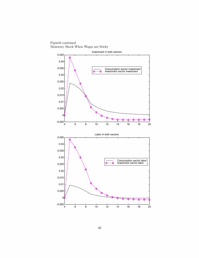
Figure6 continuedMonetary Shock When Wages are Sticky

4 6 8 10 12 14 16 18 20-0.005

0

0.005

0.01

0.015

0.02

0.025

0.03

0.035

0.04

0.045Investment in both sectors

Consumption sector investmentInvestment sector investment

4 6 8 10 12 14 16 18 20-0.005

0

0.005

0.01

0.015

0.02

0.025

0.03

0.035

0.04

0.045Labor in both sectors

Consumption sector laborInvestment sector labor

40

Figure726

Monetary Shock with Persistent and Hump Shaped Responses

4 6 8 10 12 14 16 18-0.01

0

0.01

0.02

0.03

0.04



4 6 8 10 12 14 16 18-14

-12

-10

-8

-6

-4

-2

0

2x 10




41

Figure7 continuedMonetary Shock with Persistent and Hump Shaped Responses

4 6 8 10 12 14 16 18-0.01

0

0.01

0.02

0.03

0.04

0.05



4 6 8 10 12 14 16 18-0.01

0

0.01

0.02

0.03

0.04

0.05

0.06Investment in Both Sectors


42

Sticky prices and comovement of business cycle

Documents

Transcript of Sticky prices and comovement of business cycle