PREPRINT: IEEE TRANSACTIONS SIGNAL PROCESSING, VOL. 54, NO. 11,...

PREPRINT: IEEE TRANSACTIONS SIGNAL PROCESSING, VOL. 54, NO. 11, PP. 4091–4104, NOV 2006 1

The Gaussian Mixture Probability HypothesisDensity Filter

Ba-Ngu Vo, and Wing-Kin Ma

Abstract— A new recursive algorithm is proposed for jointlyestimating the time-varying number of targets and their statesfrom a sequence of observation sets in the presence of data associ-ation uncertainty, detection uncertainty, noise and false alarms.The approach involves modelling the respective collections oftargets and measurements as random finite sets and applying theprobability hypothesis density (PHD) recursion to propagate theposterior intensity, which is a first order statistic of the randomfinite set of targets, in time. At present, there is no closed formsolution to the PHD recursion. This work shows that under linear,Gaussian assumptions on the target dynamics and birth process,the posterior intensity at any time step is a Gaussian mixture.More importantly, closed form recursions for propagating themeans, covariances and weights of the constituent Gaussiancomponents of the posterior intensity are derived. The proposedalgorithm combines these recursions with a strategy for managingthe number of Gaussian components to increase efficiency. Thisalgorithm is extended to accommodate mildly nonlinear targetdynamics using approximation strategies from the extended andunscented Kalman filters.

Index Terms— Multi-target tracking, optimal filtering, pointprocesses, random sets, intensity function.

I. I NTRODUCTION

In a multi-target environment, not only do the states of thetargets vary with time, but the number of targets also changesdue to targets appearing and disappearing. Often, not all ofthe existing targets are detected by the sensor. Moreover, thesensor also receives a set of spurious measurements (clutter)not originating from any target. As a result, the observationset at each time step is a collection of indistinguishable partialobservations, only some of which are generated by targets.The objective of multi-target tracking is to jointly estimate, ateach time step, the number of targets and their states froma sequence of noisy and cluttered observation sets. Multi-target tracking is an established area of study, for details onits techniques and applications, readers are referred to [1], [2].Up to date overviews are also available in more recent workssuch as [3]–[5].

An intrinsic problem in multi-target tracking is the unknownassociation of measurements with appropriate targets [1], [2],[6], [7]. Due to its combinatorial nature, the data associationproblem makes up the bulk of the computational load in multi-target tracking algorithms. Most traditional multi-target track-

This work is supported in part by discovery grant DP0345215 awarded bythe Australian Research Council.

B.-N. Vo is with the Electrical Engineering Department the University ofMelbourne, Melbourne, Vic. 3010, Australia. (email: [email protected]).

W.-K. Ma is with the Institute of Communications Engineering andDepartment of Electrical Engineering, National Tsing Hua University, 101,Hsinchu,Taiwan 30013. (e-mail: [email protected]).

ing formulations involve explicit associations between mea-surements and targets. Multiple Hypotheses Tracking (MHT)and its variations concern the propagation of associationhypotheses in time [2], [6], [7]. The joint probabilistic dataassociation filter (JPDAF) [1], [8], the probabilistic MHT(PMHT) [9], and the multi-target particle filter [3], [4] useobservations weighted by their association probabilities. Al-ternative formulations that avoid explicit associations betweenmeasurements and targets include Symmetric MeasurementEquations [10] and Random Finite Sets (RFS) [5], [11]–[14].

The random finite set (RFS) approach to multi-target track-ing is an emerging and promising alternative to the traditionalassociation-based methods [5], [11], [15]. A comparison of theRFS approach and traditional multi-target tracking methodshas been given in [11]. In the RFS formulation, the collectionof individual targets is treated as aset-valued state, and thecollection of individual observations is treated as aset-valuedobservation. Modelling set-valued states and set-valued obser-vations as RFSs allows the problem of dynamically estimatingmultiple targets in the presence of clutter and associationuncertainty to be cast in a Bayesian filtering framework [5],[11], [15]–[17]. This theoretically optimal approach to multi-target tracking is an elegant generalization of the single-targetBayes filter. Indeed, novel RFS-based filters such as themulti-target Bayes filter, the Probability Hypothesis Density (PHD)filter [5], [11], [18] and their implementations [16], [17], [19]–[23] have generated substantial interest.

The focus of this paper is the PHD filter, a recursion thatpropagates the first-order statistical moment, or intensity, ofthe RFS of states in time [5]. This approximation was devel-oped to alleviate the computational intractability in the multi-target Bayes filter, which stems from the combinatorial natureof the multi-target densities and the multiple integrations onthe (infinite dimensional) multi-target state space. The PHDfilter operates on the single-target state space and avoids thecombinatorial problem that arises from data association. Thesesalient features render the PHD filter extremely attractive.However, the PHD recursion involves multiple integrals thathave no closed form solutions in general. A generic sequentialMonte Carlo technique [16], [17], accompanied by variousperformance guarantees [17], [24], [25], have been proposedto propagate the posterior intensity in time. In this approach,state estimates are extracted from the particles representingthe posterior intensity using clustering techniques such asK-mean or expectation maximization. Special cases of thisso-called particle-PHD filter have also been independentlyimplemented in [21] and [22]. Due to its ability to handlethe time-varying number of nonlinear targets with relatively


low complexity, innovative extensions and applications ofthe particle-PHD filter soon followed [26]–[31]. The maindrawbacks of this approach though, are the large number ofparticles, and the unreliability of clustering techniques forextracting state estimates. (The latter will be further discussedin Section III-C.)

In this paper, we propose an analytic solution to the PHDrecursion for linear Gaussian target dynamics and Gaussianbirth model. This solution is analogous to the Kalman filteras a solution to the single-target Bayes filter. It is shownthat when the initial prior intensity is a Gaussian mixture,the posterior intensity at any subsequent time step is also aGaussian mixture. Moreover, closed form recursions for theweights, means, and covariances of the constituent Gaussiancomponents are derived. The resulting filter propagates theGaussian mixture posterior intensity in time as measurementsarrive in the same spirit as the Gaussian sum filter of [32],[33]. The fundamental difference is that the Gaussian sumfilter propagates a probability density using the Bayes recur-sion, whereas the Gaussian mixture PHD filter propagates anintensity using the PHD recursion. An added advantage ofthe Gaussian mixture representation is that it allows stateestimates to be extracted from the posterior intensity in amuch more efficient and reliable manner than clustering in theparticle-based approach. In general, the number of Gaussiancomponents in the posterior intensity increases with time.However, this problem can be effectively mitigated by keepingonly the dominant Gaussian components at each instance.Two extensions to nonlinear target dynamics models are alsoproposed. The first is based on linearizing the model while thesecond is based on the unscented transform. Simulation resultsare presented to demonstrate the capability of the proposedapproach.

Preliminary results on the closed form solution to the PHDrecursion have been presented as a conference paper [34]. Thecurrent paper is a more complete version of this work.

The structure of the paper is as follows. Section II presentsthe random finite set formulation of multi-target filtering, andthe PHD filter. Section III presents the main result of thispaper, namely the analytical solution to the PHD recursionunder linear Gaussian assumptions. An implementation of thePHD filter and simulation results are also presented. SectionIV extends the proposed approach to nonlinear models usingideas from the extended and unscented Kalman filters. Demon-strations with tracking nonlinear targets are also given. Finally,concluding remarks and possible future research directions aregiven in Section V.

II. PROBLEM FORMULATION

This section presents a formulation of multi-target filteringin the random finite set (or point process) framework. We beginwith a review of single-target Bayesian filtering in Section II-A. Using random finite set models, the multi-target trackingproblem is then formulated as a Bayesian filtering problem inSection II-B. This provides sufficient background leading toSection II-C, which describes the PHD filter.

A. Single-target filtering

In many dynamic state estimation problems, the state isassumed to follow a Markov process on the state spaceX ⊆Rnx , with transition densityfk|k−1(·|·), i.e. given a statexk−1

at timek−1, the probability density of a transition to the statexk at timek is1

fk|k−1(xk|xk−1). (1)

This Markov process is partially observed in the observationspaceZ ⊆ Rnz , as modelled by thelikelihood functiongk(·|·),i.e. given a statexk at time k, the probability density ofreceiving the observationzk ∈ Z is

gk(zk|xk). (2)

The probability density of the statexk at time k given allobservationsz1:k = (z1, . . . , zk) up to timek, denoted by

pk(xk|z1:k), (3)

is called theposterior density(or filtering density) at timek.From an initial densityp0(·), the posterior density at timekcan be computed using the Bayes recursion

pk|k−1(xk|z1:k−1) =∫

fk|k−1(xk|x)pk−1(x|z1:k−1)dx, (4)

pk(xk|z1:k) =gk(zk|xk)pk|k−1(xk|z1:k−1)∫gk(zk|x)pk|k−1(x|z1:k−1)dx

. (5)

All information about the state at timek is encapsulated in theposterior densitypk(·|z1:k), and estimates of the state at timek can be obtained using either the MMSE (Minimum MeanSquared Error) criterion or the MAP (Maximum A Posteriori)criterion2.

B. Random Finite Set Formulation of Multi-target Filtering

Now consider a multiple target scenario. LetM(k) be thenumber of targets at timek, and suppose that, at timek − 1,the target states arexk−1,1, . . . , xk−1,M(k−1) ∈ X . At thenext time step, some of these targets may die, the survivingtargets evolve to their new states, and new targets may appear.This results inM(k) new statesxk,1, . . . , xk,M(k). Note thatthe order in which the states are listed has no significancein the RFS multi-target model formulation. At the sensor,N(k) measurementszk,1, . . . , zk,N(k) ∈ Z are received attime k. The origins of the measurements are not known, andthus the order in which they appear bears no significance.Only some of these measurements are actually generatedby targets. Moreover, they are indistinguishable from thefalse measurements. The objective of multi-target trackingis to jointly estimate the number of targets and their statesfrom measurements with uncertain origins. Even in the idealcase where the sensor observes all targets and receives noclutter, single-target filtering methods are not applicable sincethere is no information about which target generated whichobservation.

1For notational simplicity, random variables and their realizations are notdistinguished.

2These criteria are not necessarily applicable to the multi-target case.


Since there is no ordering on the respective collections oftarget states and measurements at timek, they can be naturallyrepresented as finite sets, i.e.

Xk = {xk,1, . . . , xk,M(k)} ∈ F(X ), (6)

Zk = {zk,1, . . . , zk,N(k)} ∈ F(Z), (7)

whereF(X ) andF(Z) are the respective collections of allfinite subsets ofX andZ. The key in the random finite setformulation is to treat the target setXk and measurementset Zk as themulti-target stateand multi-target observationrespectively. The multi-target tracking problem can then beposed as a filtering problem with (multi-target) state spaceF(X ) and observation spaceF(Z).

In a single-target system, uncertainty is characterized bymodelling the statexk and measurementzk as random vectors.Analogously, uncertainty in a multi-target system is character-ized by modelling the multi-target stateXk and multi-targetmeasurementZk as random finite sets(RFS). An RFSXis simply a finite-set-valued random variable, which can bedescribed by a discrete probability distribution and a familyof joint probability densities [11], [35], [36]. The discretedistribution characterizes the cardinality ofX, while for agiven cardinality, an appropriate density characterizes the jointdistribution of the elements ofX.

In the following, we describe an RFS model for the timeevolution of the multi-target state, which incorporates targetmotion, birth and death. For a given multi-target stateXk−1

at timek − 1, eachxk−1 ∈ Xk−1 either continues to exist attime k with probability3 pS,k(xk−1), or dies with probability1 − pS,k (xk−1). Conditional on the existence at timek, theprobability density of a transition from statexk−1 to xk isgiven by (1), i.e.fk|k−1(xk|xk−1). Consequently, for a givenstatexk−1 ∈ Xk−1 at timek−1, its behavior at the next timestep is modelled as the RFS

Sk|k−1(xk−1) (8)

that can take on either{xk} when the target survives, or∅when the target dies. A new target at timek can arise eitherby spontaneous births (i.e. independent of any existing target)or by spawning from a target at timek−1. Given a multi-targetstateXk−1 at timek − 1, the multi-target stateXk at timekis given by the union of the surviving targets, the spawnedtargets and the spontaneous births:

Xk =

⋃

ζ∈Xk−1

Sk|k−1(ζ)

∪

⋃

ζ∈Xk−1

Bk|k−1(ζ)

∪Γk, (9)

where

Γk = RFS of spontaneous birth at timek,Bk|k−1(ζ) = RFS of targets spawned at timek from

a target with previous stateζ.

It is assumed that the RFSs constituting the union in (9)are independent of each other. The actual forms ofΓk andBk|k−1(·) are problem dependent; some examples are givenin Section III-D.

3Note thatpS,k(xk−1) is a probability parameterized byxk−1.

The RFS measurement model, which accounts for detectionuncertainty and clutter, is described as follows. A giventargetxk ∈ Xk is either detected with probability4 pD,k (xk)or missed with probability1 − pD,k (xk). Conditional ondetection, the probability density of obtaining an observationzk from xk is given by (2), i.e.gk(zk|xk). Consequently, attime k, each statexk ∈ Xk generates an RFS

Θk(xk) (10)

that can take on either{zk} when the target is detected, or∅ when the target is not detected. In addition to the targetoriginated measurements, the sensor also receives a setKk

of false measurements, or clutter. Thus, given a multi-targetstateXk at timek, the multi-target measurementZk receivedat the sensor is formed by the union of target generatedmeasurements and clutter, i.e.

Zk = Kk ∪[ ⋃

x∈Xk

Θk(x)

](11)

It is assumed that the RFSs constituting the union in (11) areindependent of each other. The actual form ofKk is problemdependent; some examples will be illustrated in Section III-D.

In a similar vein to the single-target dynamical model in(1) and (2), the randomness in the multi-target evolution andobservation described by (9) and (11) are respectively capturedin the multi-target transition densityfk|k−1(·|·) and multi-target likelihood5 gk(·|·) [5], [17]. Explicit expressions forfk|k−1(Xk|Xk−1) and gk(Zk|Xk) can be derived from theunderlying physical models of targets and sensors using FiniteSet Statistics (FISST)6 [5], [11], [15], although these are notneeded for this paper.

Let pk(·|Z1:k) denote themulti-target posterior density.Then, the optimal multi-target Bayes filter propagates themulti-target posterior in time via the recursion

pk|k−1(Xk|Z1:k−1)

=∫

fk|k−1(Xk|X)pk−1(X|Z1:k−1)µs(dX), (12)

pk(Xk|Z1:k)

=gk(Zk|Xk)pk|k−1(Xk|Z1:k−1)∫

gk(Zk|X)pk|k−1(X|Z1:k−1)µs(dX), (13)

whereµs is an appropriate reference measure onF(X ) [17],[37]. We remark that although various applications of pointprocess theory to multi-target tracking have been reported inthe literature (e.g. [38]–[40]), FISST [5], [11], [15] is the firstsystematic approach to multi-target filtering that uses RFSs inthe Bayesian framework presented above.

The recursion (12)-(13) involves multiple integrals on thespaceF(X ), which are computationally intractable. SequentialMonte Carlo implementations can be found in [16], [17],[19], [20]. However, these methods are still computationally

4Note thatpD,k(xk) is a probability parameterized byxk.5The same notation is used for multi-target and single-target densities.

There is no danger of confusion since in the single-target case the argumentsare vectors whereas in the multi-target case the arguments are finite sets.

6Strictly speaking, FISST yields the set derivative of the belief massfunctional, but this is in essence a probability density [17].


intensive due to the combinatorial nature of the densities,especially when the number of targets is large [16], [17].Nonetheless, the optimal multi-target Bayes filter has beensuccessfully applied to applications where the number oftargets is small [19].

C. The Probability Hypothesis Density (PHD) filter

The PHD filter is an approximation developed to alleviatethe computational intractability in the multi-target Bayes filter.Instead of propagating the multi-target posterior density intime, the PHD filter propagates the posterior intensity, a first-order statistical moment of the posterior multi-target state [5].This strategy is reminiscent of the constant gain Kalman filter,which propagates the first moment (the mean) of the single-target state.

For a RFSX onX with probability distributionP , its first-order moment is a non-negative functionv on X , called theintensity, such that for each regionS ⊆ X [35], [36]

∫|X ∩ S|P (dX) =

∫

S

v(x)dx. (14)

In other words, the integral ofv over any regionS givesthe expected number of elements ofX that are inS. Hence,the total massN =

∫v(x)dx gives the expected number of

elements ofX. The local maxima of the intensityv are pointsin X with the highest local concentration of expected numberof elements, and hence can be used to generate estimates forthe elements ofX. The simplest approach is to roundNand choose the resulting number of highest peaks from theintensity. The intensity is also known in the tracking literatureas the Probability Hypothesis Density (PHD) [18], [41].

An important class of RFSs, namely the Poisson RFSs, arethose completely characterized by their intensities. A RFSXis Poissonif the cardinality distribution ofX, Pr(|X| = n),is Poisson with meanN , and for any finite cardinality, theelementsx of X are independently and identically distributedaccording to the probability densityv(·)/N [35], [36]. Forthe multi-target problem described in the subsection II-B, it iscommon to model the clutter RFS [Kk in (11)] and the birthRFSs [Γk andBk|k−1(xk−1) in (9)] as Poisson RFSs.

To present the PHD filter, recall the multi-target evolutionand observation models from Section II-B with

γk(·) = intensity of the birth RFSΓk at timek,βk|k−1(·|ζ) = intensity of the RFSBk|k−1(ζ) spawned

at timek by a target with previous stateζ,pS,k(ζ) = probability that a target still exists at time

k given that its previous state isζ,pD,k(x) = probability of detection given a statex at

time k,κk(·) = intensity of the clutter RFSKk at timek

and consider the following assumptions:A.1. Each target evolves and generates observations inde-

pendently of one another,A.2. Clutter is Poisson and independent of target-originated

measurements,A.3. The predicted multi-target RFS governed bypk|k−1 is

Poisson.

Remark 1. Assumptions A.1 and A.2 are standard in mosttracking applications (see for example [1], [2]) and havealready been alluded to earlier in Section II-B. The additionalassumption A.3 is a reasonable approximation in applicationswhere interactions between targets are negligible [5]. In fact,it can be shown that A.3 is completely satisfied when there isno spawning and the RFSsXk−1 andΓk are Poisson.

Let vk and vk|k−1 denote the respective intensities associ-ated with the multi-target posterior densitypk and the multi-target predicted densitypk|k−1 in the recursion (12)-(13).Under assumptions A.1-A.3, it can be shown (using FISST [5]or classical probabilistic tools [37]) that the posterior intensitycan be propagated in time via the PHD recursion:

vk|k−1(x) =∫

pS,k(ζ)fk|k−1(x|ζ)vk−1(ζ)dζ

+∫

βk|k−1(x|ζ)vk−1(ζ)dζ + γk(x), (15)

vk(x) = [1− pD,k(x)]vk|k−1(x)

+∑

z∈Zk

pD,k(x)gk(z|x)vk|k−1(x)κk(z) +

∫pD,k(ξ)gk(z|ξ)vk|k−1(ξ)dξ

.(16)

It is clear from (15)-(16) that the PHD filter completelyavoids the combinatorial computations arising from the un-known association of measurements with appropriate targets.Furthermore, since the posterior intensity is a function on thesingle-target state spaceX , the PHD recursion requires muchless computational power than the multi-target recursion (12)-(13), which operates onF(X ). However, as mentioned in theintroduction, the PHD recursion does not admit closed formsolutions in general, and numerical integration suffers fromthe ‘curse of dimensionality.’

III. T HE PHD RECURSION FOR LINEARGAUSSIAN

MODELS

This section shows that for a certain class of multi-targetmodels, herein referred to aslinear Gaussian multi-targetmodels, the PHD recursion (15)-(16) admits a closed formsolution. This result is then used to develop an efficient multi-target tracking algorithm. The linear Gaussian multi-targetmodels are specified in Section III-A, while the solution tothe PHD recursion is presented in Section III-B. Implementa-tion issues are addressed in Section III-C. Numerical resultsare presented in Section III-D and some generalizations arediscussed in Section III-E.

A. Linear Gaussian multi-target model

Our closed form solution to the PHD recursion requires,in addition to assumptions A.1-A.3, a linear Gaussian multi-target model. Along with the standard linear Gaussian modelfor individual targets, the linear Gaussian multi-target modelincludes certain assumptions on the birth, death and detectionof targets. These are summarized below:

A.4. Each target follows a linear Gaussian dynamical modeland the sensor has a linear Gaussian measurement model, i.e.

fk|k−1(x|ζ) = N (x; Fk−1ζ, Qk−1), (17)

gk(z|x) = N (z; Hkx,Rk), (18)


whereN (·;m, P ) denotes a Gaussian density with meanmand covarianceP , Fk−1 is the state transition matrix,Qk−1

is the process noise covariance,Hk is the observation matrix,andRk is the observation noise covariance.

A.5. The survival and detection probabilities are state inde-pendent, i.e.

pS,k(x) = pS,k, (19)

pD,k(x) = pD,k. (20)

A.6. The intensities of the birth and spawn RFSs areGaussian mixtures of the form

γk(x) =Jγ,k∑

i=1

w(i)γ,kN (x; m(i)

γ,k, P(i)γ,k), (21)

βk|k−1(x|ζ) =Jβ,k∑

j=1

w(j)β,kN (x; F (j)

β,k−1ζ + d(j)β,k−1, Q

(j)β,k−1),

(22)

where Jγ,k, w(i)γ,k, m

(i)γ,k, P

(i)γ,k, i = 1, . . . , Jγ,k, are given

model parameters that determine the shape of the birth in-tensity; similarly, Jβ,k, w

(j)β,k, F

(j)β,k−1, d

(j)β,k−1, and Q

(j)β,k−1,

j = 1, . . . , Jβ,k, determine the shape of the spawning intensityof a target with previous stateζ.

Some remarks regarding the above assumptions are in order:Remark 2. Assumptions A.4 and A.5 are commonly used

in many tracking algorithms [1], [2]. For clarity in the pre-sentation, we only focus on state independentpS,k andpD,k,although closed form PHD recursions can be derived for moregeneral cases (see Subsection III-E).

Remark 3. In assumption A.6,m(i)γ,k, i = 1, ..., Jγ,k are the

peaks of the spontaneous birth intensity in (21). These pointshave the highest local concentrations of expected number ofspontaneous births, and represent, for example, airbases orairports where targets are most likely to appear. The covariancematrix P

(i)γ,k determines the spread of the birth intensity in

the vicinity of the peakm(i)γ,k. The weight w(i)

γ,k gives the

expected number of new targets originating fromm(i)γ,k. A

similar interpretation applies to (22), the spawning intensityof a target with previous stateζ, except that thejth peak,F

(j)β,k−1ζ + d

(j)β,k−1, is an affine function ofζ. Usually, a

spawned target is modelled to be in the proximity of its parent.For example,ζ could correspond to the state of an aircraftcarrier at timek− 1, while F

(j)β,k−1ζ + d

(j)β,k−1 is the expected

state of fighter planes spawned at timek. Note that other formsof birth and spawning intensities can be approximated, to anydesired accuracy, using Gaussian mixtures [42].

B. The Gaussian mixture PHD recursion

For the linear Gaussian multi-target model, the followingtwo propositions present a closed form solution to the PHDrecursion (15)-(16). More concisely, these propositions showhow the Gaussian components of the posterior intensity areanalytically propagated to the next time.

Proposition 1 Suppose that Assumptions A.4-A.6 hold andthat the posterior intensity at timek−1 is a Gaussian mixture

of the form

vk−1(x) =Jk−1∑

i=1

w(i)k−1N (x; m(i)

k−1, P(i)k−1). (23)

Then, the predicted intensity for timek is also a Gaussianmixture, and is given by

vk|k−1(x) = vS,k|k−1(x) + vβ,k|k−1(x) + γk(x), (24)

whereγk(x) is given in (21),

vS,k|k−1(x) = pS,k

Jk−1∑

j=1

w(j)k−1N (x; m(j)

S,k|k−1, P(j)S,k|k−1), (25)

m(j)S,k|k−1 = Fk−1m

(j)k−1, (26)

P(j)S,k|k−1 = Qk−1 + Fk−1P

(j)k−1F

Tk−1, (27)

vβ,k|k−1(x) =Jk−1∑

j=1

Jβ,k∑

`=1

w(j)k−1w

(`)β,kN (x;m(j,`)

β,k|k−1, P(j,`)β,k|k−1),

(28)

m(j,`)β,k|k−1 = F

(`)β,k−1m

(j)k−1 + d

(`)β,k−1, (29)

P(j,`)β,k|k−1 = Q

(`)β,k−1 + F

(`)β,k−1P

(j)β,k−1(F

(`)β,k−1)

T (30)

Proposition 2 Suppose that Assumptions A.4-A.6 hold andthat the predicted intensity for timek is a Gaussian mixtureof the form

vk|k−1(x) =Jk|k−1∑

i=1

w(i)k|k−1N (x; m(i)

k|k−1, P(i)k|k−1). (31)

Then, the posterior intensity at timek is also a Gaussianmixture, and is given by

vk(x) = (1− pD,k)vk|k−1(x) +∑

z∈Zk

vD,k(x; z), (32)

where

vD,k(x; z) =Jk|k−1∑

j=1

w(j)k (z)N (x;m(j)

k|k(z), P (j)k|k), (33)

w(j)k (z) =

pD,k w(j)k|k−1q

(j)k (z)

κk(z) + pD,k

∑Jk|k−1

`=1 w(`)k|k−1q

(`)k (z)

, (34)

q(j)k (z) = N (z;Hkm

(j)k|k−1, Rk + HkP

(j)k|k−1H

Tk ), (35)

m(j)k|k(z) = m

(j)k|k−1 + K

(j)k (z −Hkm

(j)k|k−1), (36)

P(j)k|k = [I −K

(j)k Hk]P (j)

k|k−1, (37)

K(j)k = P

(j)k|k−1H

Tk (HkP

(j)k|k−1H

Tk + Rk)−1. (38)

Propositions 1 and 2 can be established by applying thefollowing standard results for Gaussian functions:

Lemma 1 Given F , d, Q, m, and P of appropriate dimen-sions, and thatQ and P are positive definite,∫N (x; Fζ+d,Q)N (ζ; m,P )dζ = N (x; Fm+d,Q+FPFT )

(39)


Lemma 2 GivenH, R, m, andP of appropriate dimensions,and thatR and P are positive definite,

N (z; Hx,R)N (x;m,P ) = q(z)N (x; m, P ) (40)

where

q(z) = N (z; Hm,R + HPHT ) (41)

m = m + K(z −Hm) (42)

P = (I −KH)P (43)

K = PHT (HPHT + R)−1 (44)

Note that Lemma 1 can be derived from Lemma 2, which inturn can be found in [43] or [44] (Section 3.8), though in aslightly different form.

Proposition 1 is established by substituting (17), (19), (21),(22) and (23) into the PHD prediction (15), and replacingintegrals of the form (39) by appropriate Gaussians as givenby Lemma 1. Similarly, Proposition 2 is established by substi-tuting (18), (20) and (31) into the PHD update (16), and thenreplacing integrals of the form (39) and product of Gaussiansof the form (40) by appropriate Gaussians as given by Lemmas1 and 2 respectively.

It follows by induction from Propositions 1 and 2 that if theinitial prior intensityv0 is a Gaussian mixture (including thecase wherev0 = 0), then all subsequent predicted intensitiesvk|k−1 and posterior intensitiesvk are also Gaussian mixtures.Proposition 1 provides closed form expressions for computingthe means, covariances and weights ofvk|k−1 from those ofvk−1. Proposition 2 then provides closed form expressions forcomputing the means, covariances and weights ofvk fromthose of vk|k−1 when a new set of measurements arrives.Propositions 1 and 2 are, respectively, the prediction andupdate steps of the PHD recursion for a linear Gaussian multi-target model, herein referred to as theGaussian mixture PHDrecursion. For completeness, we summarize the key steps ofthe Gaussian mixture PHD filter in Table I.

Remark 4. The predicted intensityvk|k−1 in Proposition1 consists of three termsvS,k|k−1, vβ,k|k−1 and γk due,respectively, to the existing targets, the spawned targets, andthe spontaneous births. Similarly, the updated posterior in-tensity vk in Proposition 2 consists of a mis-detection term,(1 − pD,k)vk|k−1, and |Zk| detection terms,vD,k(·; z), onefor each measurementz ∈ Zk. As it turns out, the recursionsfor the means and covariances ofvS,k|k−1 and vβ,k|k−1 areKalman predictions, and the recursions for the means andcovariances ofvD,k(·; z) are Kalman updates.

Given the Gaussian mixture intensitiesvk|k−1 and vk, thecorresponding expected number of targetsNk|k−1 andNk canbe obtained by summing up the appropriate weights. Proposi-tions 1 and 2 lead to the following closed form recursions forNk|k−1 and Nk:

Corollary 1 Under the premises of Proposition 1, the meanof the predicted number of targets is

Nk|k−1 = Nk−1

pS,k+

Jβ,k∑

j=1

w(j)β,k

+

Jγ,k∑

j=1

w(j)γ,k, (45)

TABLE I

PSEUDO-CODE FOR THEGAUSSIAN MIXTURE PHD FILTER.

given {w(i)k−1, m

(i)k−1, P

(i)k−1}

Jk−1

i=1 , and the measurement set Zk .step 1. (prediction for birth targets)

i = 0.for j = 1, . . . , Jγ,k

i := i + 1.w

(i)k|k−1

= w(j)γ,k

, m(i)k|k−1

= m(j)γ,k

, P(i)k|k−1

= P(j)γ,k

.endfor j = 1, . . . , Jβ,k

for ` = 1, . . . , Jk−1

i := i + 1.w

(i)k|k−1

= w(`)k−1w

(j)β,k

,

m(i)k|k−1

= d(j)β,k−1 + F

(j)β,k−1m

(`)k−1,

P(i)k|k−1

= Q(j)β,k−1 + F

(j)β,k−1P

(`)k−1(F

(j)β,k−1)

T .

endend

step 2. (prediction for existing targets)

for j = 1, . . . , Jk−1

i := i + 1.w

(i)k|k−1

= pS,k w(j)k−1,

m(i)k|k−1

= Fk−1m(j)k−1, P

(i)k|k−1

= Qk−1+Fk−1P(j)k−1F T

k−1,endJk|k−1 = i.

step 3. (construction of PHD update components)

for j = 1, . . . , Jk|k−1

η(j)k|k−1

= Hkm(j)k|k−1

, S(j)k

= Rk + HkP(j)k|k−1

HTk

,

K(j)k

= P(j)k|k−1

HTk

[S(j)k

]−1, P(j)k|k

= [I − K(j)k

Hk]P(j)k|k−1

.end

step 4. (update)

for j = 1, . . . , Jk|k−1

w(j)k

= (1 − pD,k)w(j)k|k−1

,

m(j)k

= m(j)k|k−1

, P(j)k

= P(j)k|k−1

.end` := 0.for each z ∈ Zk

` := ` + 1.for j = 1, . . . , Jk|k−1

w(`Jk|k−1

+j)

k= pD,k w

(j)k|k−1

N (z; η(j)k|k−1

, S(j)k

).

m(`Jk|k−1

+j)

k= m

(j)k|k−1

+ K(j)k

(z − η(j)k|k−1

),

P(`Jk|k−1

+j)

k= P

(j)k|k

,

end

w(`Jk|k−1

+j)

k:=

w(`Jk|k−1

+j)

k

κk(z) +�Jk|k−1

i=1 w(`Jk|k−1

+i)

k

, for j =

1, . . . , Jk|k−1.endJk = `Jk|k−1 + Jk|k−1.

output {w(i)k

, m(i)k

, P(i)k

}Jk

i=1.

Corollary 2 Under the premises of Proposition 2, the meanof the updated number of targets is

Nk = Nk|k−1(1− pD,k) +∑

z∈Zk

Jk|k−1∑

j=1

w(j)k (z) (46)


In Corollary 1, the mean of the predicted number of targetsis obtained by adding the mean number of surviving targets,the mean number of spawnings and the mean number of births.A similar interpretation can be drawn from Corollary 2. Whenthere is no clutter, the mean of the updated number of targets isthe number of measurements plus the mean number of targetsthat are not detected.

C. Implementation issues

The Gaussian mixture PHD filter is similar to the Gaussiansum filter of [32], [33] in the sense that they both propagateGaussian mixtures in time. Like the Gaussian sum filter, theGaussian mixture PHD filter also suffers from computationproblems associated with the increasing number of Gaussiancomponents as time progresses. Indeed, at timek, the Gaussianmixture PHD filter requires

(Jk−1(1 + Jβ,k) + Jγ,k)(1 + |Zk|) = O(Jk−1|Zk|)Gaussian components to representvk, whereJk−1 is numberof components ofvk−1. This implies the number of compo-nents in the posterior intensities increases without bound.

A simple pruning procedure can be used to reduce thenumber of Gaussian components propagated to the next timestep. A good approximation to the Gaussian mixture posteriorintensity

vk(x) =Jk∑

i=1

w(i)k N (x; m(i)

k , P(i)k )

can be obtained by truncating components that have weakweights w

(i)k . This can be done by discarding those with

weights below some preset threshold, or by keeping only a cer-tain number of components with strongest weights. Moreover,some of the Gaussian components are so close together thatthey could be accurately approximated by a single Gaussian.Hence, in practice these components can be merged into one.These ideas lead to the simple heuristic pruning algorithmshown in Table II.

Having computed the posterior intensityvk, the next taskis to extract multi-target state estimates. In general, such atask may not be simple. For example, in the particle-PHDfilter [17], the estimated number of targetsNk is given bythe total mass of the particles representingvk. The estimatedstates are then obtained by partitioning these particles intoNk clusters, using standard clustering algorithms. This workswell when the posterior intensityvk naturally hasNk clusters.Conversely, whenNk differs from the number of clusters, thestate estimates become unreliable.

In the Gaussian mixture representation of the posteriorintensity vk, extraction of multi-target state estimates isstraightforward since the means of the constituent Gaussiancomponents are indeed the local maxima ofvk, provided thatthey are reasonably well-separated. Note that after pruning(see Table II) closely spaced Gaussian components would havebeen merged. Since the height of each peak depends on boththe weight and covariance, selecting theNk highest peaks ofvk may result in state estimates that correspond to Gaussianswith weak weights. This is not desirable because the expected

TABLE II

PRUNING FOR THEGAUSSIAN MIXTURE PHD FILTER.

given {w(i)k

, m(i)k

, P(i)k

}Jk

i=1, a truncation threshold T , a merging thresh-old U , and a maximum allowable number of Gaussian terms Jmax.Set ` = 0, and I = {i = 1, . . . , Jk|w

(i)k

> T}.repeat

` := ` + 1.j := arg max

i∈Iw

(i)k

.

L :=�i ∈ I ��(m

(i)k

− m(j)k

)T (P(i)k

)−1(m(i)k

− m(j)k

) ≤ U�.w

(`)k

=�i∈L

w(i)k

.

m(`)k

= 1

w(`)k

�i∈L

w(i)k

x(i)k

.

P(`)k

= 1

w(`)k

�i∈L

w(i)k

(P(i)k

+ (m(`)k

− m(i)k

)(m(`)k

− m(i)k

)T ).

I := I\L.

until I = ∅.if ` > Jmax then replace {w

(i)k

, m(i)k

, P(i)k

}`i=1 by those of the Jmax

Gaussians with largest weights.output {w(i)

k, m

(i)k

, P(i)k

}`i=1 as pruned Gaussian components.

TABLE III

MULTI -TARGET STATE EXTRACTION

given {w(i)k

, m(i)k

, P(i)k

}Jk

i=1.Set Xk = ∅.for i = 1, . . . , Jk

if w(i)k

> 0.5,

for j = 1, . . . , round(w(i)k

)

update Xk :=�Xk , m

(i)k �

end

end

endoutput Xk as the multi-target state estimate.

number of targets due to these peaks is small, even though themagnitudes of the peaks are large. A better alternative is toselect the means of the Gaussians that have weights greaterthan some threshold e.g.0.5. This state estimation procedurefor the Gaussian mixture PHD filter is summarized in Table III.

D. Simulation Results

Two simulation examples are used to test the proposedGaussian mixture PHD filter. An additional example can befound in [34].

1) Example 1: For illustration purposes, consider a two-dimensional scenario with an unknown and time varyingnumber of targets observed in clutter over the surveillanceregion [−1000, 1000]× [−1000, 1000] (in m). The statexk =[ px,k, py,k, px,k, py,k ]T of each target consists of position(px,k, py,k) and velocity(px,k, py,k), while the measurementis a noisy version of the position.

Each target has survival probabilitypS,k = 0.99, andfollows the linear Gaussian dynamics (17) with


Fk =[I2 ∆I2

02 I2

], Qk = σ2

ν

[∆4

4 I2∆3

2 I2∆3

2 I2 ∆2I2

],

where In and 0n denotes, respectively, then × n identityand zero matrices,∆ = 1s is the sampling period, andσν = 5(m/s2) is the standard deviation of the process noise.Targets can appear from two possible locations as well asspawned from other targets. Specifically, a Poisson RFSΓk

with intensity

γk(x) = 0.1N (x; m(1)γ , Pγ) + 0.1N (x; m(2)

γ , Pγ),

where

m(1)γ = [ 250, 250, 0, 0 ]T ,

m(2)γ = [ − 250,−250, 0, 0 ]T ,

Pγ = diag([ 100, 100, 25, 25 ]T ),

is used to model spontaneous births in the vicinity ofm(1)γ

andm(2)γ . Additionally, the RFSBk|k−1(ζ) of targets spawned

from a target with previous stateζ is Poisson with intensity

βk|k−1(x|ζ) = 0.05N (x; ζ, Qβ),

Qβ = diag([ 100, 100, 400, 400 ]T ).

Each target is detected with probabilitypD,k = 0.98, andthe measurement follows the observation model (18) withHk = [ I2 02 ], Rk = σ2

εI2, where σε = 10m is thestandard deviation of the measurement noise. The detectedmeasurements are immersed in clutter that can be modelledas a Poisson RFSKk with intensity

κk(z) = λcV u(z), (47)

whereu(·) is the uniform density over the surveillance region,V = 4×106m2 is the ‘volume’ of the surveillance region, andλc = 12.5×10−6m−2 is the average number of clutter returnsper unit volume (i.e. 50 clutter returns over the surveillanceregion).

−400 −200 0 200 400 600 800 1000−1000

−800

−600

−400

−200

0

200

400

Target 1; born at k=1; dies at k=100



x coordinate (in m)

y co

ordi

nate

(in

m)

Fig. 1. Target trajectories. ‘◦’– locations at which targets are born; ‘¤’–locations at which targets die.

Figure 1 shows the true target trajectories, while Figure 2plots these trajectories with cluttered measurements against

time. Targets 1 and 2 are born at the same time but at twodifferent locations. They travel along straight lines (their trackscross atk = 53s) and atk = 66s target 1 spawns target 3.

10 20 30 40 50 60 70 80 90 100−1000

−500

0

500

1000

time step

x co

ordi

nate

(in

m) True tracks

Measurements

(a)

10 20 30 40 50 60 70 80 90 100−1000

−500

0

500

1000

time step

y co

ordi

nate

(in

m)

(b)

Fig. 2. Measurements and true target positions.

10 20 30 40 50 60 70 80 90 100−1000

−500

0

500

1000

time step

x co

ordi

nate

(in

m)

PHD filter estimates True tracks

(a)

10 20 30 40 50 60 70 80 90 100−1000

−500

0

500

1000

time step

y co

ordi

nate

(in

m)

(b)

Fig. 3. Position estimates of the Gaussian mixture PHD filter.

The Gaussian mixture PHD filter, with parametersT =10−5, U = 4, andJmax = 100 (see Table II for the meaningsof these parameters) is applied. From the position estimatesshown in Figure 3, it can be seen that the Gaussian mixturePHD filter provides accurate tracking performance. The filternot only successfully detects and tracks targets 1 and 2,but also manages to detect and track the spawned target 3.The filter does generate anomalous estimates occasionally, butthese false estimates die out very quickly.

2) Example 2:In this example we evaluate the performanceof the Gaussian mixture PHD filter by benchmarking it againstthe JPDA filter [1], [8] via Monte Carlo simulations. TheJPDA filter is a classical filter for tracking a known and fixednumber of targets in clutter. In a scenario where the number oftargets is constant, the JPDA filter (given the correct numberof targets) is expected to outperform the PHD filter, since thelatter has neither knowledge of the number of targets, nor evenknowledge that the number of targets is constant. For thesereasons, the JPDA filter serves as a good benchmark.


The experiment settings are the same as those of Example1, but without spawning, as the JPDA filter requires a knownand fixed number of targets. The true tracks in this exampleare those of targets 1 and 2 in Figure 1. Target trajectoriesare fixed for all simulation trials, while observation noise andclutter are independently generated at each trial.

We study track loss performance by using the following cir-cular position error probability (CPEP) (see [45] for example)

CPEPk(r) =1|Xk|

∑

x∈Xk

ρk(x, r),

for some position error radiusr, where

ρk(x, r) = Prob{‖Hx−Hx‖2 > r for all x ∈ Xk},H = [ I2 02 ] and‖·‖2 is the2-norm. In addition, we measurethe expected absolute error on the number of targets for theGaussian mixture PHD filter:

E{| |Xk| − |Xk| |}.Note that standard performance measures such as the meansquare distance error are not applicable to multi-target filtersthat jointly estimate the number of targets and their states (suchas the PHD filter).

1 2 3 4 5 6 7 8 9 10

x 10−5

0

0.2

0.4

0.6

0.8

1

E{||X

k|−

|Xk||}

(tim

eav

erag

ed)

λc (a)

1 2 3 4 5 6 7 8 9 10

x 10−5

0

0.2

0.4

0.6

0.8

1Gaussian Mixture PHDJPDA

CP

EP

k(r

)(t

ime

aver

aged

)

λc (b)

Fig. 4. Tracking performance versus clutter rate. The detection probabilityis fixed atpD,k = 0.98. The CPEP radius isr = 20m.

Figure 4 shows the tracking performance of the two filtersfor various clutter ratesλc [cf., Eq. (47)] with the CPEPradius fixed atr = 20m. Observe that the CPEPs of the twofilters are quite close for a wide range of clutter rates. Thisis rather surprising considering that the JPDA filter has exactknowledge of the number of targets. Figure 4(a) suggests thatthe occasional overestimation/underestimation of the numberof targets is not significant in the Gaussian mixture PHD filter.

Figure 5 shows the tracking performance for various valuesof detection probabilitypD,k with the clutter rate fixed atλc =12.5× 10−6m−2. Observe that the performance gap betweenthe two filters increases aspD,k decreases. This is becausethe PHD filter has to resolve higher detection uncertainty ontop of uncertainty in the number of targets. When detectionuncertainty increases (pD,k decreases), uncertainty about thenumber of targets also increases. In contrast, the JPDA filter’s

0.7 0.75 0.8 0.85 0.9 0.95 10

0.2

0.4

0.6

0.8

1

E{||X

k|−

|Xk||}

(tim

eav

erag

ed)

pD,k (a)

0.7 0.75 0.8 0.85 0.9 0.95 10

0.2

0.4

0.6

0.8

1

CP

EP

k(r

)(t

ime

aver

aged

)

pD,k (b)

Fig. 5. Tracking performance versus detection probability. The clutter rateis fixed atλc = 12.5× 10−6m−2. The CPEP radius isr = 20m.

exact knowledge of the number of targets is not affected bythe increase in detection uncertainty.

E. Generalizations to exponential mixturepD,k and pS,k

As remarked in Section III-A, closed form solutions to thePHD recursion can still be obtained for a certain class of state-dependent probability of survival and probability of detection.Indeed, Propositions 1 and 2 can be easily generalized tohandlepS,k(x) andpD,k(x) of the forms:

pS,k(ζ) = w(0)S,k +

JS,k∑

j=1

w(j)S,kN (ζ; m(j)

S,k, P(j)S,k), (48)

pD,k(x) = w(0)D,k +

JD,k∑

j=1

w(j)D,kN (x; m(j)

D,k, P(j)D,k), (49)

whereJS,k, w(0)S,k, w

(i)S,k, m

(i)S,k, P

(i)S,k, i = 1, ..., JS,k andJD,k,

w(0)D,k, w

(i)D,k, m

(i)D,k, P

(i)D,k, i = 1, ..., JD,k are given model

parameters such thatpS,k(x) and pD,k(x) lie between 0 and1 for all x.

The closed form predicted intensityvk|k−1 can be obtainedby applying Lemma 2 to convertpS,k(ζ)vk−1(ζ) into aGaussian mixture, which is then integrated with the transitiondensityfk|k−1(x|ζ) using Lemma 1. The closed form updatedintensity vk can be obtained by applying Lemma 2 onceto pD,k(x)vk|k−1(x) and twice topD,k(x)gk(x|z)vk|k−1(x)to convert these products to Gaussian mixtures. For com-pleteness, the Gaussian mixture expressions forvk|k−1 andvk are given in the following Propositions, although theirimplementations will not be pursued.

Proposition 3 Under the premises of Proposition 1, withpS,k(x) given by (48) instead of (19), the predicted intensityvk|k−1 is given by (24) but with

vS,k|k−1(x) =Jk−1∑

i=1

JS,k∑

j=0

w(i,j)S,k|k−1N (x; m(i,j)

S,k|k−1, P(i,j)S,k|k−1)

(50)


w(i,j)S,k|k−1 = w

(i)k−1w

(j)S,kq

(i,j)k−1 ,

m(i,j)S,k|k−1 = Fk−1m

(i,j)k−1 ,

P(i,j)S,k|k−1 = Qk−1 + Fk−1P

(i,j)k−1 FT

k−1,

q(i,0)k−1 = 1, m

(i,0)k−1 = m

(i)k−1, P

(i,0)k−1 = P

(i)k−1,

q(i,j)k−1 = N (m(j)

S,k; m(i)k−1, P

(j)S,k + P

(i)k−1),

m(i,j)k−1 = m

(i)k−1 + K

(i,j)k−1 (m(j)

S,k −m(i)k−1),

P(i,j)k−1 = (I −K

(i,j)k−1 )P (i)

k−1,

K(i,j)k−1 = P

(i)k−1(P

(i)k−1 + P

(j)S,k)−1.

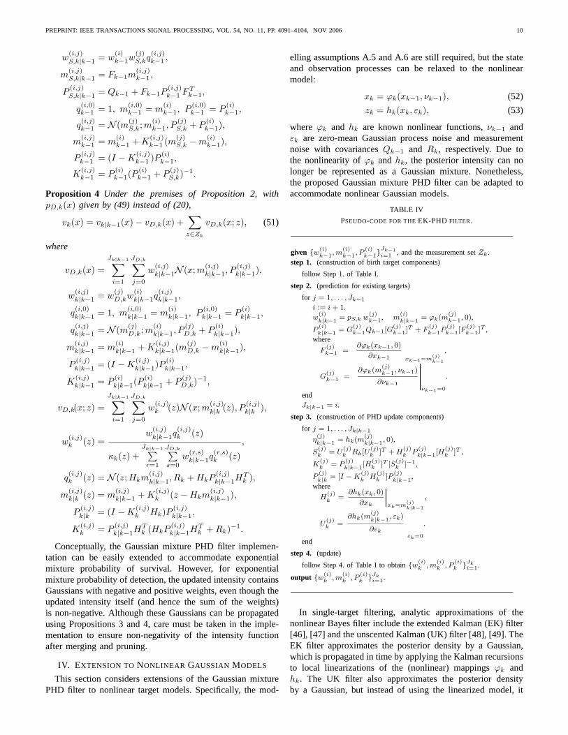
Proposition 4 Under the premises of Proposition 2, withpD,k(x) given by (49) instead of (20),

vk(x) = vk|k−1(x)− vD,k(x) +∑

z∈Zk

vD,k(x; z), (51)

where

vD,k(x) =Jk|k−1∑

i=1

JD,k∑

j=0

w(i,j)k|k−1N (x;m(i,j)

k|k−1, P(i,j)k|k−1),

w(i,j)k|k−1 = w

(j)D,kw

(i)k|k−1q

(i,j)k|k−1,

q(i,0)k|k−1 = 1, m

(i,0)k|k−1 = m

(i)k|k−1, P

(i,0)k|k−1 = P

(i)k|k−1,

q(i,j)k|k−1 = N (m(j)

D,k; m(i)k|k−1, P

(j)D,k + P

(i)k|k−1),

m(i,j)k|k−1 = m

(i)k|k−1 + K

(i,j)k|k−1(m

(j)D,k −m

(i)k|k−1),

P(i,j)k|k−1 = (I −K

(i,j)k|k−1)P

(i)k|k−1,

K(i,j)k|k−1 = P

(i)k|k−1(P

(i)k|k−1 + P

(j)D,k)−1,

vD,k(x; z) =Jk|k−1∑

i=1

JD,k∑

j=0

w(i,j)k (z)N (x; m(i,j)

k|k (z), P (i,j)k|k ),

w(i,j)k (z) =

w(i,j)k|k−1q

(i,j)k (z)

κk(z) +Jk|k−1∑

r=1

JD,k∑s=0

w(r,s)k|k−1q

(r,s)k (z)

,

q(i,j)k (z) = N (z; Hkm

(i,j)k|k−1, Rk + HkP

(i,j)k|k−1H

Tk ),

m(i,j)k|k (z) = m

(i,j)k|k−1 + K

(i,j)k (z −Hkm

(i,j)k|k−1),

P(i,j)k|k = (I −K

(i,j)k Hk)P (i,j)

k|k−1,

K(i,j)k = P

(i,j)k|k−1H

Tk (HkP

(i,j)k|k−1H

Tk + Rk)−1.

Conceptually, the Gaussian mixture PHD filter implemen-tation can be easily extended to accommodate exponentialmixture probability of survival. However, for exponentialmixture probability of detection, the updated intensity containsGaussians with negative and positive weights, even though theupdated intensity itself (and hence the sum of the weights)is non-negative. Although these Gaussians can be propagatedusing Propositions 3 and 4, care must be taken in the imple-mentation to ensure non-negativity of the intensity functionafter merging and pruning.

IV. EXTENSION TO NONLINEAR GAUSSIAN MODELS

This section considers extensions of the Gaussian mixturePHD filter to nonlinear target models. Specifically, the mod-

elling assumptions A.5 and A.6 are still required, but the stateand observation processes can be relaxed to the nonlinearmodel:

xk = ϕk(xk−1, νk−1), (52)

zk = hk(xk, εk), (53)

where ϕk and hk are known nonlinear functions,νk−1 andεk are zero-mean Gaussian process noise and measurementnoise with covariancesQk−1 and Rk, respectively. Due tothe nonlinearity ofϕk and hk, the posterior intensity can nolonger be represented as a Gaussian mixture. Nonetheless,the proposed Gaussian mixture PHD filter can be adapted toaccommodate nonlinear Gaussian models.

TABLE IV

PSEUDO-CODE FOR THEEK-PHD FILTER.

given {w(i)k−1, m

(i)k−1, P

(i)k−1}

Jk−1

i=1 , and the measurement set Zk .step 1. (construction of birth target components)

follow Step 1. of Table I.

step 2. (prediction for existing targets)

for j = 1, . . . , Jk−1

i := i + 1.w

(i)k|k−1

= pS,k w(j)k−1, m

(i)k|k−1

= ϕk(m(j)k−1, 0),

P(i)k|k−1

= G(j)k−1Qk−1[G

(j)k−1]

T + F(j)k−1P

(j)k−1[F

(j)k−1]

T ,where

F(j)k−1 =

∂ϕk(xk−1, 0)

∂xk−1

��xk−1=m

(j)k−1

,

G(j)k−1 =

∂ϕk(m(j)k−1, νk−1)

∂νk−1

��νk−1=0

.

endJk|k−1 = i.

step 3. (construction of PHD update components)

for j = 1, . . . , Jk|k−1

η(j)k|k−1

= hk(m(j)k|k−1

, 0),

S(j)k

= U(j)k

Rk[U(j)k

]T + H(j)k

P(j)k|k−1

[H(j)k

]T ,

K(j)k

= P(j)k|k−1

[H(j)k

]T [S(j)k

]−1,

P(j)k|k

= [I − K(j)k

H(j)k

]P(j)k|k−1

,where

H(j)k

=∂hk(xk, 0)

∂xk

��xk=m

(j)k|k−1

,

U(j)k

=∂hk(m

(j)k|k−1

, εk)

∂εk

��εk=0

.

end

step 4. (update)

follow Step 4. of Table I to obtain {w(i)k

, m(i)k

, P(i)k

}Jki=1.

output {w(i)k

, m(i)k

, P(i)k

}Jki=1.

In single-target filtering, analytic approximations of thenonlinear Bayes filter include the extended Kalman (EK) filter[46], [47] and the unscented Kalman (UK) filter [48], [49]. TheEK filter approximates the posterior density by a Gaussian,which is propagated in time by applying the Kalman recursionsto local linearizations of the (nonlinear) mappingsϕk andhk. The UK filter also approximates the posterior densityby a Gaussian, but instead of using the linearized model, it


computes the Gaussian approximation of the posterior densityat the next time step using the unscented transform. Detailsfor the EK and UK filters are given in [46], [47] and [48],[49], respectively.

TABLE V

PSEUDO-CODE FOR THEUK-PHD FILTER.

given {w(i)k−1, m

(i)k−1, P

(i)k−1}

Jk−1

i=1 and the measurement set Zk .step 1. (construction of birth target components)

follow Step 1. of Table I.for j = 1, . . . , i

- set

µ :=

�m

(j)k|k−1

0 �, C :=

�P

(j)k|k−1

0

0 Rk�.- use the unscented transformation (see [46], [47]) with mean µ

and covariance C to generate a set of sigma points and weights,denoted by {y

(`)k

, u(`)}L`=0.

- partition y(`)k

= [ (x(`)k|k−1

)T , (ε(`)k

)T ]T for ` = 0, 1, . . . , L.- compute

z(`)k|k−1

:= hk(x(`)k|k−1

, ε(`)k

), ` = 0, . . . , L,

η(j)k|k−1

=�L

`=0u(`)z

(`)k|k−1

,

S(j)k

=�L

`=0u(`)(z

(`)k|k−1

− η(j)k|k−1

)(z(`)k|k−1

− η(j)k|k−1

)T ,

G(j)k

=�L

`=0u(`)(x

(`)k|k−1

−m(j)k|k−1

)(z(`)k|k−1

−η(j)k|k−1

)T ,

K(j)k

= G(j)k

[S(j)k

]−1,

P(j)k|k

= P(j)k|k−1

− G(j)k

[S(j)k

]−1[G(j)k

]T .

end

step 2. (construction of existing target components)

for j = 1, . . . , Jk−1

- i := i + 1.- w

(i)k|k−1

= pS,k w(j)k−1.

- set

µ := ��m(i)k−1

0

0

��, C := ��P (i)k−1 0 0

0 Qk−1 0

0 0 Rk

��.

- use the unscented transformation with mean µ and covarianceC to generate a set of sigma points and weights, denoted by{y

(`)k

, u(`)}L`=0.

- partition y(`)k

= [ (x(`)k−1)

T , (ν(`)k−1)T , (ε

(`)k

)T ]T for ` =

0, 1, . . . , L.- compute

x(`)k|k−1

:= ϕk(x(`)k−1, ν

(`)k−1), ` = 0, . . . , L,

z(`)k|k−1

:= hk(x(`)k|k−1

, ε(`)k

), ` = 0, . . . , L,

m(i)k|k−1

=�L

`=0u(`)x

(`)k|k−1

,

P(i)k|k−1

=�L

`=0u(`)(x

(`)k|k−1

−m(j)k|k−1

)(x(`)k|k−1

−m(j)k|k−1

)T ,

η(i)k|k−1

=�L

`=0u(`)z

(`)k|k−1

,

S(i)k

=�L

`=0u(`)(z

(`)k|k−1

− η(j)k|k−1

)(z(`)k|k−1

− η(j)k|k−1

)T ,

G(i)k

=�L

`=0u(`)(x

(`)k|k−1

−m(j)k|k−1

)(z(`)k|k−1

−η(j)k|k−1

)T ,

K(i)k

= G(i)k

[S(i)k

]−1,

P(i)k|k

= P(i)k|k−1

− G(i)k

[S(i)k

]−1[G(i)k

]T .

endJk|k−1 = i.

step 3. (update)

follow Step 4. of Table I to obtain {w(i)k

, m(i)k

, P(i)k

}Jk

i=1.

output {w(i)k

, m(i)k

, P(i)k

}Jk

i=1.

Following the development in Section III-B, it can be shownthat the posterior intensity of the multi-target state propagatedby the PHD recursions (15)-(16) is a weighted sum of variousfunctions, many of which are non-Gaussian. In the same veinas the EK and UK filters, we can approximate each of thesenon-Gaussian constituent functions by a Gaussian. Adoptingthe philosophy of the EK filter, an approximation of theposterior intensity at the next time step can then be obtainedby applying the Gaussian mixture PHD recursions to a locallylinearized target model. Alternatively, in a similar manner tothe UK filter, the unscented transform can be used to computethe components of the Gaussian mixture approximation of theposterior intensity at the next time step. In both cases, theweights of these components are also approximations.

Based on the above observations, we propose two nonlinearGaussian mixture PHD filter implementations, namely, theextended Kalman PHD(EK-PHD) filter and theunscentedKalman PHD(UK-PHD) filter. Given that details for the EKand UK filters have been well-documented in the literature(see e.g. [44], [46]–[49]), the developments for the EK-PHDand UK-PHD filters are conceptually straightforward, thoughnotationally cumbersome, and will be omitted. However, forcompleteness, the key steps in these two filters are summarizedas pseudo codes in Tables IV and V, respectively.

Remark 5. Similar to its single-target counterpart, theEK-PHD filter is only applicable to differentiable nonlinearmodels. Moreover, calculating the Jacobian matrices may betedious and error-prone. The UK-PHD filter, on the other hand,does not suffer from these restrictions and can even be appliedto models with discontinuities.

Remark 6. Unlike the particle-PHD filter, where the particleapproximation converges (in a certain sense) to the posteriorintensity as the number of particle tends to infinity [17], [24],this type of guarantee has not been established for the EK-PHD or UK-PHD filter. Nonetheless, for mildly nonlinearproblems, the EK-PHD and UK-PHD filters provide goodapproximations and are computationally cheaper than theparticle-PHD filter, which requires a large number of particlesand the additional cost of clustering to extract multi-target stateestimates.

A. Simulation Results for a Nonlinear Gaussian Example

In this example, each target has a survival probabilitypS,k =0.99 and follows a nonlinear nearly-constant turn model [50]in which the target state takes the formxk = [ yT

k , ωk ]T ,whereyk = [ px,k, py,k, px,k, py,k ]T , andωk is the turn rate.The state dynamics are given by

yk = F (ωk−1)yk−1 + Gwk−1,

ωk = ωk−1 + ∆uk−1,

where

F (ω) =

1 0 sin ω∆ω − 1−cos ω∆

ω

0 1 1−cos ω∆ω

sin ω∆ω

0 0 cos ω∆ − sinω∆0 0 sin ω∆ cos ω∆

, G =

∆2

2 00 ∆2

2∆ 00 ∆

,


∆ = 1s, wk ∼ N (·; 0, σ2wI2), σw = 15m/s2, and uk ∼

N (·; 0, σ2u), σu = (π/180)rad/s. We assume no spawning,

and that the spontaneous birth RFS is Poisson with intensity

γk(x) = 0.1N (x; m(1)γ , Pγ) + 0.1N (x; m(2)

γ , Pγ),

where

m(1)γ = [ − 1000, 500, 0, 0, 0 ]T ,

m(2)γ = [ 1050, 1070, 0, 0, 0 ]T ,

Pγ = diag([ 2500, 2500, 2500, 2500, (6× π180 )2 ]T ).

Each target has a probability of detectionpD,k = 0.98. Anobservation consists of bearing and range measurements

zk =

[arctan(px,k/py,k)√

p2x,k + p2

y,k

]+ εk,

where εk ∼ N (·; 0, Rk) with Rk = diag([σ2θ , σ2

r ]T ), σθ =2 × (π/180)rad/s and σr = 20m. The clutter RFS followsthe uniform Poisson model in (47) over the surveillance region[−π/2, π/2]rad× [0, 2000]m, with λc = 3.2×10−3(radm)−1

(i.e. an average of 20 clutter returns on the surveillance region).The true target trajectories are plotted in Figure 6. Targets

1 and 2 appear from 2 different locations, 5s apart. They bothtravel in straight lines before making turns atk = 16s. Thetracks almost cross atk = 25s, and the targets resume theirstraight trajectories afterk = 34s. The pruning parameters forthe UK-PHD and EK-PHD filters areT = 1× 10−5, U = 4,and Jmax = 100. The results, shown in Figures 7 and 8,indicate that both the UK-PHD and EK-PHD filters exhibitgood tracking performance.

−1000 −500 0 500 10000

200

400

600

800

1000

1200



x coordinate (in m)

y co

ordi

nate

(in

m)

Fig. 6. Target trajectories. ‘◦’– locations at which targets are born; ‘¤’–locations at which targets die.

In many nonlinear Bayes filtering applications, the UK filterhas shown better performance than the EK filter [49]. Thesame is expected in nonlinear PHD filtering. However, thisexample only has a mild nonlinearity and the performancegap between the EK-PHD and UK-PHD filters may not benoticeable.

V. CONCLUSIONS

Closed form solutions to the PHD recursion are importantanalytical and computational tools in multi-target filtering.Under linear Gaussian assumptions, we have shown that whenthe initial prior intensity of the random finite set of targets isa Gaussian mixture, the posterior intensity at any time step is

5 10 15 20 25 30 35 40 45

−1000

−500

0

500

1000

time step

x co

ordi

nate

(in

m) PHD filter estimates

True tracks

(a)

5 10 15 20 25 30 35 40 450

500

1000

1500

2000

2500

time step

y co

ordi

nate

(in

m)

(b)

Fig. 7. Position estimates of the EK-PHD filter.

5 10 15 20 25 30 35 40 45

−1000

−500

0

500

1000

time step

x co

ordi

nate

(in

m) PHD filter estimates

True tracks

(a)

5 10 15 20 25 30 35 40 450

500

1000

1500

2000

2500

time step

y co

ordi

nate

(in

m)

(b)

Fig. 8. Position estimates of the UK-PHD filter.

also a Gaussian mixture. More importantly, we have derivedclosed form recursions for the weights, means, and covariancesof the constituent Gaussian components of the posterior inten-sity. An implementation of the PHD filter has been proposedby combining the closed form recursions with a simple pruningprocedure to manage the growing number of components. Twoextensions to nonlinear models using approximation strategiesfrom the extended Kalman filter and the unscented Kalmanfilter have also been proposed. Simulations have demonstratedthe capabilities of these filters to track an unknown and time-varying number of targets under detection uncertainty and falsealarms.

There are a number of possible future research directions.Closed formed solutions to the PHD recursion for jumpMarkov linear models are being investigated. In highly non-linear, non-Gaussian models, where particle implementationsare required, the EK-PHD and UK-PHD filters are obviouscandidates for efficient proposal functions that can improveperformance. This also opens up the question of optimalimportance functions and their approximations. The efficiencyand simplicity in implementation of the Gaussian mixturePHD recursion also suggest possible application to trackingin sensor networks.


REFERENCES

[1] Y. Bar-Shalom and T. E. Fortmann,Tracking and Data Association.Academic Press, San Diego, 1988.

[2] S. Blackman,Multiple Target Tracking with Radar Applications. ArtechHouse, Norwood, 1986.

[3] C. Hue, J. P. Lecadre, and P. Perez, “Sequential Monte Carlo methodsfor multiple target tracking and data fusion,”IEEE Trans. Trans. SP,vol. 50, no. 2, pp. 309–325, 2002.

[4] ——, “Tracking multiple objects with particle filtering,”IEEE Trans.AES, vol. 38, no. 3, pp. 791–812, 2002.

[5] R. Mahler, “Multi-target Bayes filtering via first-order multi-targetmoments,”IEEE Trans. AES, vol. 39, no. 4, pp. 1152–1178, 2003.

[6] D. Reid, “An algorithm for tracking multiple targets,”IEEE Trans. AC,vol. AC-24, no. 6, pp. 843–854, 1979.

[7] S. Blackman, “Multiple hypothesis tracking for multiple target tracking,”IEEE A & E Systems Magazine, vol. 19, no. 1, part 2, pp. 5–18, 2004.

[8] T. E., Fortmann, Y. Bar-Shalom, and M. Scheffe, “Sonar tracking ofmultiple targets using joint probabilistic data association,”IEEE J.Oceanic Eng., vol. OE-8, no. July, pp. 173–184, 1983.

[9] R. L. Streit and T. E. Luginbuhl, “Maximum likelihood method forprobabilistic multi-hypothesis tracking,” inProc. SPIE, vol. 2235, pp.5–7, 1994.

[10] E. W. Kamen, “Multiple target tracking based on symmetric measure-ment equations,”IEEE Trans. AC, vol. AC-37, pp. 371–374, 1992.

[11] I. Goodman, R. Mahler, and H. Nguyen,Mathematics of Data Fusion.Kluwer Academic Publishers, 1997.

[12] R. Mahler, “Random sets in information fusion: An overview,” inRandom Sets: Theory and Applications,J. Goutsias et. al. (eds.),Springer Verlag, pp. 129–164, 1997.

[13] ——, “Multi-target moments and their application to multi-target track-ing,” in Proc. Workshop on Estimation, Tracking and Fusion:A tributeto Yaakov Bar-Shalom, Monterey, pp. 134–166, 2001.

[14] ——, “Random set theory for target tracking and identification,” inDataFusion Hand Book,D. Hall and J. Llinas (eds.), CRC press Boca Raton,pp. 14/1–14/33, 2001.

[15] ——, “An introduction to multisource-multitarget statistics and applica-tions,” Lockheed Martin Technical Monograph, 2000.

[16] B. Vo, S. Singh, and A. Doucet, “Sequential Monte Carlo implementa-tion of the PHD filter for multi-target tracking,” inProc. Int’l Conf. onInformation Fusion,Cairns, Australia, pp. 792–799, 2003.

[17] ——, “Sequential Monte Carlo methods for multi-target filtering withrandom finite sets,”IEEE Trans. Aerospace and Electronic Systems,vol. 41, no. 4, pp. 1224–1245, 2005, also: http://www.ee.unimelb.edu.au/staff/bv/publications.html.

[18] R. Mahler, “A theoretical foundation for the Stein-Winter ProbabilityHypothesis Density (PHD) multi-target tracking approach,” inProc.2002 MSS Nat’l Symp. on Sensor and Data Fusion, vol. 1, (Unclassified)Sandia National Laboratories, San Antonio TX, 2000.

[19] W.-K. Ma, B. Vo, S. Singh, and A. Baddeley, “Tracking an unknowntime-varying number of speakers using TDOA measurements: A randomfinite set approach,”IEEE Trans. Signal Processing, vol. 54, no. 9, pp.3291–3304, Sept 2006.

[20] H. Sidenbladh and S. Wirkander, “Tracking random sets of vehiclesin terrain,” in Proc. 2003 IEEE Workshop on Multi-Object Tracking,Madison Wisconsin, 2003.

[21] H. Sidenbladh, “Multi-target particle filtering for the Probability Hy-pothesis Density,” inProc. Int’l Conf. on Information Fusion,Cairns,Australia, pp. 800–806, 2003.

[22] T. Zajic and R. Mahler, “A particle-systems implementation of the PHDmulti-target tracking filter,” inSignal Processing, Sensor Fusion andTarget Recognition XII, SPIE Proc., vol. 5096, pp. 291–299, 2003.

[23] M. Vihola, “Random sets for multitarget tracking and data association,”Licentiate thesis, Dept. Inform. Tech. & Inst. Math., Tampere Univ.Technology, Finland, Aug. 2004.

[24] A. Johansen, S. Singh, A. Doucet, and B. Vo, “Convergence of thesequential Monte Carlo implementation of the PHD filter,”Methodologyand Computing in Applied Probability, vol. 8, no. 2, pp. 265-291, 2006.

[25] D. Clark and J. Bell, “Convergence results for the Particle-PHD filter,”IEEE Trans. Signal Processing,vol. 54, no. 7, pp. 26522661, 2006.

[26] K. Panta, B. Vo, S. Singh, and A. Doucet, “Probability HypothesisDensity filter versus multiple hypothesis tracking,” inI. Kadar (ed.),Signal Processing, Sensor Fusion, and Target Recognition XIII, Proc.SPIE, vol. 5429, pp. 284–295, 2004.

[27] L. Lin, Y. Bar-Shalom, and T. Kirubarajan, “Data association combinedwith the Probability Hypothesis Density filter for multitarget tracking,”in O. E. Drummond (ed.) Signal and Data Processing of Small Targets,Proc. SPIE, vol. 5428, pp. 464–475, 2004.

[28] K. Punithakumar, T. Kirubarajan, and A. Sinha, “A multiple modelProbability Hypothesis Density filter for tracking maneuvering targets,”in O. E. Drummond (ed.) Signal and Data Processing of Small Targets,Proc. SPIE, vol. 5428, pp. 113–121, 2004.

[29] P. Shoenfeld, “A particle filter algorithm for the multi-target ProbabilityHypothesis Density,” inI. Kadar (ed.), Signal Processing, SensorFusion, and Target Recognition XIII, Proc. SPIE, vol. 5429, pp. 315–325, 2004.

[30] M. Tobias and A. D. Lanterman, “Probability Hypothesis Density-basedmultitarget tracking with bistatic range and Doppler observations,”IEEProc. Radar Sonar and Navigation, vol. 152, no. 3, pp. 195–205, 2005.

[31] D. Clark and J. Bell, “Bayesian multiple target tracking in forwardscan sonar images using the PHD filter,”IEE Proc. Radar Sonar andNavigation, vol. 152, no. 5, pp. 327–334, 2005.

[32] H. W. Sorenson and D. L. Alspach, “Recursive Bayesian estimationusing Gaussian sum,”Automatica, vol. 7, pp. 465–479, 1971.

[33] D. L. Alspach and H. W. Sorenson, “Nonlinear Bayesian estimationusing Gaussian sum approximations,”IEEE Trans. AC, vol. AC-17,no. 4, pp. 439–448, 1972.

[34] B. Vo and W.-K. Ma, “A closed-form solution to the ProbabilityHypothesis Density filter,” inProc. Int’l Conf. on Information Fusion,Philadelphia, 2005.

[35] D. Daley and D. Vere-Jones,An introduction to the theory of pointprocesses. Springer-Verlag, 1988.

[36] D. Stoyan, D. Kendall, and J. Mecke,Stochastic Geometry and itsApplications. John Wiley & Sons, 1995.

[37] B. Vo and S. Singh, “Technical aspects of the Probability HypothesisDensity recursion,”Tech. Rep. TR05-006EEE Dept. The University ofMelbourne, Australia, 2005.

[38] S. Mori, C. Chong, E. Tse, and R. Wishner, “Tracking and identifyingmultiple targets without apriori identifications,”IEEE Trans. AC, vol.AC-21, pp. 401–409, 1986.

[39] R. Washburn, “A random point process approach to multi-object track-ing,” in Proc. American Control Conf., vol. 3, pp. 1846–1852, 1987.

[40] N. Portenko, H. Salehi, and A. Skorokhod, “On optimal filtering ofmultitarget systems based on point process observations,”RandomOperators and Stochastic Equations, vol. 5, no. 1, pp. 1–34, 1997.

[41] M. C. Stein and C. L. Winter, “An adaptive theory of probabilisticevidence accrual,”Los Alamos National Laboratotries Report,LA-UR-93-3336, 1993.

[42] J. T.-H. Lo, “Finite-dimensional sensor orbits and optimal non-linearfiltering,” IEEE Trans. IT, vol. IT-18, no. 5, pp. 583–588, 1972.

[43] Y. C. Ho and R. C. K. Lee, “A Bayesian approach to problems instochastic estimation and control,”IEEE Trans. AC, vol. AC-9, pp. 333–339, 1964.

[44] B. Ristic, S. Arulampalam, and N. Gordon,Beyond the Kalman Filter:Particle Filters for Tracking Applications. Artec House, 2004.

[45] Y. Ruan and P. Willett, “The Turbo PMHT,”IEEE Trans. AES, vol. 40,no. 4, pp. 1388–1398, 2004.

[46] A. H. Jazwinski,Stochastic Processes and Filtering Theory. AcademicPress, New York, 1970.

[47] B. D. Anderson and J. B. Moore,Optimal Filtering. Prentice-Hall,New Jersey, 1979.

[48] S. J. Julier and J. K. Uhlmann, “A new extension of the Kalmanfilter to nonlinear systems,” inProc. AeroSense: 11th Int’l Symp. onAerospace/Defence Sensing, Simulation and Controls,Orlando, Florida,1997.

[49] ——, “Unscented filtering and nonlinear estimation,” inProc. IEEE,vol. 92, no. 3, pp. 401–422, 2004.

[50] X.-R. Li and V. Jilkov, “Survey of maneuvering target tracking,”IEEETrans. AES, vol. 39, no. 4, pp. 1333–1364, 2003.

PREPRINT: IEEE TRANSACTIONS SIGNAL PROCESSING, VOL. 54, NO. 11,...

Documents

Transcript of PREPRINT: IEEE TRANSACTIONS SIGNAL PROCESSING, VOL. 54, NO. 11,...