(Preprint) AAS 14-427

IMPACT PROBABILITY ANALYSIS FOR NEAR-EARTH OBJECTSIN EARTH RESONANT ORBITS

George Vardaxis∗ and Bong Wie†

Accurate estimation of the impact probability of near-Earth objects (NEOs) is re-quired for planning a space mission to mitigate their threat. There are severalmethods that can be used to determine the odds of an asteroid impacting the planet.Methods incorporating analytic encounter geometry analyses, target B-planes, andanalytic keyhole and resonant orbit theory are useful in the sense that they canaid in obtaining a quick rough estimation of the impact probability. Other meth-ods using high-precision orbital dynamic simulations, taking into account non-conservative perturbations, allow for a better, more accurate estimate of the im-pact probability. Taking the advantages of a direct numerical simulation approach,incorporating analytic keyhole theory, this paper presents a new computational ap-proach to accurately estimating the impact probability of NEOs, especially thosein Earth resonant orbits.

INTRODUCTION

Asteroids impacting the Earth is a very real and ever-present possibility. The ability to determinethe likelihood of such an impact to a certain degree of certainty is a necessity in order to counteracttheir imposing threat. When it comes to near Earth asteroids, there are three major components toany design or mission involving these asteroids: identification, determination, and mitigation. A lotof effort has been made to identify as many threats to the Earth as early as possible. At the AsteroidDeflection Research Center, there has been a lot of work done on the mitigation component bystudying potential mission designs to deflect and/or disrupt hazardous asteroids. The focus of thispaper is on the second of the three components mentioned previously, the orbit determination of theasteroids.

The ability to determine the orbit of a potentially hazardous near-Earth asteroids is very important.In this paper, techniques including a high precision gravitational simulator, encounter geometry,target planes, and keyholes are used to help evaluate the orbits that an asteroid has the potential ofgetting into and their associated impact probability. Upon acquisition of an asteroid, a high-fidelitygravitational model can be used to propagate an asteroid’s state into the future to see if/when itwould come in close proximity to another body. Encounters with planets would most likely resultin the asteroid’s orbit changing. Based on the encounter’s geometry, the resulting heliocentric orbitcould be in resonance with the encounter planet that would result in another encounter, or impact.Using the encounter’s target plane and keyhole theory, an estimate on the current and future impactprobability between the asteroid and the planet can be made. While each of these techniques can be∗Graduate Research Assistant, Asteroid Deflection Research Center, Department of Aerospace Engineering, Iowa StateUniversity, 2348 Howe Hall, Ames, IA 50011-2271, USA.†Vance Coffman Endowed Chair Professor, Asteroid Deflection Research Center, Department of Aerospace Engineering,Iowa State University, 2271 Howe Hall, Ames, IA 50011-2271, USA.

1

useful on their own, the combination of them should prove to be more useful as more informationcan be conveyed at once.

ORBIT DETERMINATION

NASA had to find ways to increase the rate of discovery of near-Earth objects (NEOs), by decreeof Congress in 1990. Through their efforts, objects of significant size, have been found on occasionto be on a potential Earth-impacting trajectory. Often requiring high-fidelity N-body models, con-taining the effects of non-gravitational orbital perturbations such as solar radiation pressure (SRP),the accurate prediction of such Earth-impacting trajectories could be found. Such highly precise as-teroid orbits allows mission designers to take advantage of more specific mission planning, highercertainty of the target’s location, and more accurate impact probability.

Orbit Simulation

The orbital motion of an asteroid is governed by a so-called Standard Dynamical Model (SDM)of the form [1]

d2~r

dt2= − µ

r3~r +

n∑k=1

µk

(~rk − ~r|~rk − ~r|3

− ~rkr3k

)+ ~f (1)

where µ = GM is the gravitational parameter of the Sun, n is the number of perturbing bodies, µkand ~rk are the gravitational parameter and heliocentric position vector of perturbing body k, respec-tively, and ~f represents other non-conservative orbital perturbation acceleration. The gravitationalmodel used in orbit propagation takes into account the effects of the Sun, all eight planets, Pluto,Ceres, Pallas, and Vesta.

Previous studies performed at the ADRC were concerned with the impact probability of po-tential Earth-impacting asteroids, such as 99942 Apophis. Using commercial software such asNASA’s General Mission Analysis Tool (GMAT), AGI’s Satellite Tool Kit (STK), and Jim Baer’sComet/asteroid Orbit Determination and Ephemeris Software (CODES), the ADRC conducted pre-cision orbital simulation studies to compare with JPL’s Sentry program [2].

At the moment, the three asteroids of study at the ADRC for high precision orbit propagationare Apophis, 1999 RQ36, and 2011 AG5, due to their proximity to Earth and their relatively highimpact probability. Apophis and 2011 AG5, recently declared to have virtually no threat to Earth,are primarily used for validation of the numerical integration and orbit propagation schemes in theADRC’s N-body simulator.

Previous Work

Taking Apophis as a reference NEO, simulations have been run from an an initial epoch of August27, 2011 until January 1, 2037 to show the capabilities of the ADRC’s N-body code in calculatingprecise, long-term orbit trajectories. A preliminary test was conducted for the period of May 23,2029 to May 13, 2036 show the relative errors of GMAT and STK to JPL’s Sentry (Horizons),as well as the error of the N-body code with respect to Sentry. The error in the radial position ofApophis between the N-body code to that of JPL’s Sentry is much lower than that of both GMAT andSTK. The N-body simulator used to obtain the aforementioned results uses a Runge-Kutta Fehlberg(RKF) 7(8) fixed-time-step method, including the orbital perturbations of all eight planets, Pluto,and Earth’s Moon, in the form of constant orbital element rates coupled with the nominal elementvalues provided updated position and velocity data for the perturbation bodies [2].

2

Current Work and Capabilities

Expanding upon the work done on the numerical integration scheme used to obtain the resultspreviously discussed, the fixed-time-step numerical integration algorithm has been changed to avariable step method. The Runge-Kutta Fehlberg method is used for approximating the solutionof a differential equation x(t) = f(x,t) with initial condition x(t0). The implementation evaluatesf(x,t) thirteen times per step using embedded seventh order and eight order Runge-Kutta estimatesto estimate not only the solution but also the error. By specifying the interval in which the resultsof the integration should be reported and the acceptable local error tolerance, the algorithm takes asmany error controlled steps as necessary to calculate the state vector at the desired time.

Using ephemeris data from the NASA Jet Propulsion Laboratory (JPL) Horizons website, orbitaldata for all these bodies is taken for a given period of time to construct a planetary state vector(X,Y, Z, VX , VY , VZ) database. In order to accommodate the need to retrieve data at any specifieddate within the propagation time, a Lagrange interpolation scheme is constructed. Using the JulianDate of the available state vector data for each planet as the distinct independent variables of an nth

degree Lagrange interpolating polynomial, a unique polynomial P (x) is created for each time step,which is then applied to each body.

As far as non-conservative perturbations, the three most well-known are solar radiation pressure(SRP), relativistic effects, and the Yarkovsky effect, the former two being the most prevalent effects.Solar radiation pressure provides a radial outward force on the asteroid body from the interaction ofthe Sun’s photons impacting the asteroid surface. The SRP model is given by

aSRP = (K)(CR)

(AR

M

)(LS

4πcr2

)⇒ ~aSRP = (K)(CR)

(AR

M

)(LS

4πcr3

)~r (2)

where~aR and aR are the solar radiation pressure acceleration vector and its magnitude, respectively,CR is the coefficient for solar radiation, AR is the cross-sectional area presented to the Sun, M isthe mass of the asteroid, K is the fraction of the solar disk visible at the asteroid’s location, LS isthe luminosity of the Sun, c is the speed of light, and ~r and r is the distance vector and magnitudeof the asteroid from the Sun, respectively.

The relativistic effects of the body are included because for many objects, especially those withsmall semimajor axes and large eccentricities, those effects introduce a non-negligible radial accel-eration toward the Sun. One form of the relativistic effects is represented by

~aR =k2

c2r3

[4k2~r

r−(~r · ~r

)~r + 4

(~r · ~r

)~r

](3)

where ~aR is the acceleration vector due to relativistic effects, k is the Gaussian constant, ~r is theposition vector of the asteroid, and ~r is the velocity vector of the asteroid. With the introductionof such non-conservative forces the error within the system will increase, but these effects need tobe included in calculations in order to maintain consistency with the planetary ephemeris. A morecomplete dynamical model will allow the accurate calculation of asteroid impact probabilities andgravitational keyholes, leading to more effective mission designs [3].

ORBITAL ENCOUNTER GEOMETRIES

When a body undergoes an encounter with a planet, there are a number ways that its orbit willbe affected. The environment around a planet is very dynamic in nature, and small inaccuracies

3

Figure 1. Reference frame of ~U . The origin is placed at the planet’s center, thepositive x-axis is opposite the direction of the Sun, the y-axis is in the direction of theplanet’s motion, and the z-axis is parallel to the planet’s angular momentum vector.The angles φ and θ define the direction of ~U .

in modeling can result in drastic differences between the simulated trajectories and the actual tra-jectory. Getting a good understanding behind the geometry of planetary close-approaches and theeffect that they have on the orbital elements of the bodies that undergo them should assist with thetask of predicting the resulting orbital trajectory after a close flyby of a planet.

Basic Assumptions

The dynamical system under consideration in the following analysis consists of the Sun, a planetorbiting the Sun on a circular orbit, and an asteroid, viewed as a particle, that is on an eccentric andinclined orbit around the Sun that crosses the orbit of the planet. Assume the planet has an orbitalradius R = 1, the product k

√M = 1, where k is the Gaussian constant and M is the mass of the

Sun, and the asteroid has orbital parameters (a, e, i, ω,Ω). In order to have the asteroid cross theorbital path of the planet, the asteroid must meet the following criteria: a(1 − e) < 1 < a(1 + e).The frame of reference established for this analysis is centered on the planet, the x-axis pointsradially opposite to the Sun, the y-axis is the direction of motion of the planet itself, and the z-axisis completes the right-handed system by pointing in the direction of the planet’s angular momentumvector. The three most important orbital elements used in the analysis are the heliocentric orbitalelements semi-major axis a, eccentricity e, and inclination i, of the approaching body [4].

Relationship Between Orbital Parameters a, e, i and U , φ, θ

Let U = (Ux, Uy, Uz) and U be the relative velocity vector and magnitude between the planetand the asteroid [4], defined as

4

U =

√3−

[1

a+ 2√a(1− e2) cos i

](4)

Ux = U sin θ sinφ (5)

Uy = U cos θ (6)

Uz = U sin θ cosφ (7)

where θ and φ define the angles that define the direction of U by

φ = tan−1

[±

√2a− 1

a2(1− e2)− 1

1

sin i

](8)

θ = cos−1[

1− U2 − 1/a

2U

](9)

where θ may vary between 0 and π, and φ between -π/2 and π/2.

In terms of a, e, and i, the components of U are given by

Ux =

[2− 1

a− a(1− e2)

]1/2(10)

Uy =√a(1− e2) cos i− 1 (11)

Uz =√a(1− e2) sin i (12)

and, inversely, we have

a =1

1− U2 − 2Uy(13)

e =[U4 + 4U2

y + U2x(1− U2 − 2Uy) + 4U2Uy

]1/2 (14)

i = sin−1√U2z /[U

2z + (1 + Uy)2] (15)

Post-Encounter Geometry

After the asteroid has an encounter with the target planet, the U vector is rotated by an angle γ inthe direction ψ, where ψ is the angle measured counter-clockwise from the meridian containing theU vector. The deflection angle γ is related to the encounter parameter b by

tan1

2γ =

m

bU2(16)

where m is the mass of the planet, in units of the Sun’s mass. The angle θ after the encounter,denoted by θ′, is calculated from

cos θ′ = cos θ cos γ + sin θ sin γ cosψ (17)

and, defining ξ = φ− φ′, we have

sin ξ = sinψ sin γ/ sin θ′ (18)

cos ξ = (cos γ sin θ − sin γ cos θ cosψ)/ sin θ′ (19)

tan ξ = sinψ sin γ/(cos γ sin θ − sin γ cos θ cosψ) (20)

tanφ′ = (tanφ− tan ξ)/(1 + tanφ tan ξ) (21)

5

Evaluating for the post-encounter variables θ′ and φ′, the values of a′, e′, and i′ can be obtainedaccordingly [4]. Figure 2 pictorially represents the relationship between the pre-encounter (U , θ, φ)and post-encounter (U ′, θ′, φ′) variables that make up the geometry of a body’s encounter [4].

X

Y

Z

U U' γ

ψ ϕ ϕ'

χ

θ' θ

Figure 2. Reference frame of U and U’. After an encounter with a planet, the vectorU is rotated by and angle γ in the direction of ψ.

POST-ENCOUNTER ORBITAL TRAJECTORY

Based on the encounter geometry analysis, the orbital variations for a body are shown via surfaceplots like the ones in the previous section. The amount of the orbit change depends on the speedthe body has relative to the planet and how close it gets, but it is possible to find the varied orbitaltrajectory of the body after encounter. Short of using a high-fidelity gravitational model to trackthe progress of the body through numerical integration, the encounter phase can be modeled astwo-body motion governed by the planet as the central body.

During a flyby of a planet, the incoming and outgoing v-infinity vectors and the pre- and post-encounter heliocentric velocities connect at the flyby planet through the following relationships

~v−∞ = ~vfb,pre − ~vpre (22)

~v+∞ = ~vpost − ~vfb,post (23)

where ~v−∞ and ~v+∞ are the incoming and outgoing v-infinity vectors, respectively, ~vfb,pre and ~vfb,postare the velocities of the flyby planet upon entry and exit of the planetary sphere of influence, and~vpre and ~vpost are the heliocentric velocity vectors entering and leaving the sphere of influence of theplanet, respectively. During the encounter, the planet will turn body through an angle φ, determinedby

φ = 2 arcsin1

1 + rpv2∞/µ(24)

where rp is the periapse radius of the flyby hyperbola, v∞ is the magnitude of the incoming v-infinityvector, and µ is the gravitational parameter of the flyby planet [5].

6

The heliocentric speed gained by the body through the planetary encounter and the heliocentricdelta-v vector caused by the flyby can be determined through the following two equations

δv = 2v∞/e (25)

δ~v = ~vpre − ~vpost (26)

where e is the eccentricity of the flyby hyperbola [5]. Numerically, the following nonlinear equalitypath constraint must be true to ensure that no laws of physics are violated.

|~v−∞| − |~v+∞| = 0 (27)

The resulting difference from the constraint may not necessarily be zero, however, a small toleranceof error can be allowed.

Regardless of the analysis conducted here being done analytically or numerically, the resultsshould be rather similar. Thus, given the pre- and post-encounter heliocentric velocity vectors ofthe body, along with their respective heliocentric position vectors, the orbital elements of the helio-centric orbits can be found and compared to see just how much the orbit of the body has changed.Beyond seeing just how much the heliocentric trajectory would be changed due to the planetaryclose encounter, the data on orbital variations can be used to find resonance orbits.

The key parameter for resonant return orbits is the post-encounter semi-major axis. Scalingeverything so that the Earth-Sun distance and the Sun’s gravitational constant are equal to 1

T 2/a3 ≈ 4π2 (28)

where T and a are the period and semi-major axis of the body, respectively, in nondimensionalunits. Given that Earth’s orbital period is 2π, the encountering body’s post-encounter orbital periodis 2π(a′)3/2, where a′ is the post-encounter semi-major axis. If the Earth and post-encounter body’speriods are commensurable, then after h periods of the asteroid and k periods of the Earth havepassed, where k and h are integers, a new encounter will take place as

(a′)3/2 = k/h (29)

Picking a number of Earth orbits to elapse, and an acceptable tolerance for the orbital ratio (k/h),the number of asteroid orbits can be found that would correspond to a resonance orbit existingbetween the asteroid and Earth from a given post-encounter semi-major axis.

ANALYTIC KEYHOLE THEORY

To this point, high-precision gravitational simulation, orbital encounter geometries, and post-encounter orbital trajectories have been discussed. To complete the discussion, the topic of targetplanes and keyholes must be discussed. Upon every encounter, the asteroid passes through whatis known as a target plane. On these target planes can exist what are called keyholes, and if theasteroid were to pass through said keyhole, it would return on a resonant return orbit and impact theplanet. The following describes the theory behind target planes and analytic keyhole computation.

7

Target Planes

A target plane is defined as a geocentric plane oriented to be normal to the asteroid’s geocentricvelocity vector. By observing the point of intersection of an asteroid trajectory with the target planecan lend significant insight into the nature of a future encounter. In general, there are two distinctplanes and several coordinate systems that can be used in such a framework. The classical targetplane is referred to as the B-plane, which has been used in astrodynamics since the 1960s. TheB-plane is oriented normal to the incoming asymptote of the geocentric hyperbola, or normal to theunperturbed relative velocity ~v∞. The plane’s name is a reference to the so-called impact parameterb, the distance from the geocenter to the intercept of the asymptote on this plane, known as theminimum encounter distance along the unperturbed trajectory [6]. Figure 3 depicts the relationshipbetween the target B-plane and the trajectory plane of the asteroid. The system of coordinates thatwill be used for the analyses conducted in this paper are described later, those shown on the figureare just an example that could be used.

Figure 3. Representation of the target B-plane of a planet with respect to the incomingapproach of a body on the trajectory plane.

Target Plane Coordinates

Generally it is convention to place the origin of the B-plane’s coordinate system at the geocenter,but the orientation of the coordinate axes on the plane is arbitrary. The system has been fixed attimes by aligning the axes in a way so that one of the nominal target plane coordinates is zero, orby aligning one of the coordinate axes with either the projection of the Earth’s polar axis or theprojection of the Earth’s heliocentric velocity.

One of the most important functions of the target plane is to determine whether a collision ispossible, and if not, how deep the encounter will be. With the B-plane, we obtain the minimumdistance of the unperturbed asteroid orbit at its closest approach point with the Earth - the impactparameter b. That single variable however does not tell whether the asteroid’s perturbed trajectorywill intersect the image of the Earth on the following encounter, but the information can be extracted

8

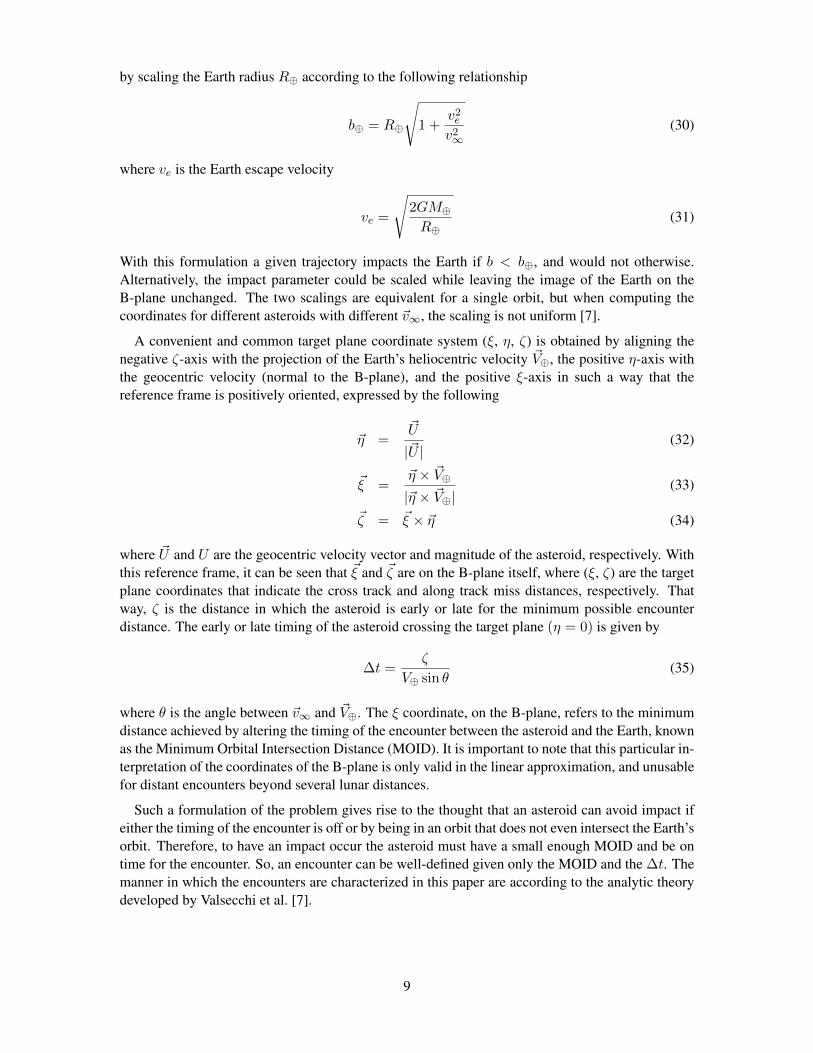
by scaling the Earth radius R⊕ according to the following relationship

b⊕ = R⊕

√1 +

v2ev2∞

(30)

where ve is the Earth escape velocity

ve =

√2GM⊕R⊕

(31)

With this formulation a given trajectory impacts the Earth if b < b⊕, and would not otherwise.Alternatively, the impact parameter could be scaled while leaving the image of the Earth on theB-plane unchanged. The two scalings are equivalent for a single orbit, but when computing thecoordinates for different asteroids with different ~v∞, the scaling is not uniform [7].

A convenient and common target plane coordinate system (ξ, η, ζ) is obtained by aligning thenegative ζ-axis with the projection of the Earth’s heliocentric velocity ~V⊕, the positive η-axis withthe geocentric velocity (normal to the B-plane), and the positive ξ-axis in such a way that thereference frame is positively oriented, expressed by the following

~η =~U

|~U |(32)

~ξ =~η × ~V⊕

|~η × ~V⊕|(33)

~ζ = ~ξ × ~η (34)

where ~U and U are the geocentric velocity vector and magnitude of the asteroid, respectively. Withthis reference frame, it can be seen that ~ξ and ~ζ are on the B-plane itself, where (ξ, ζ) are the targetplane coordinates that indicate the cross track and along track miss distances, respectively. Thatway, ζ is the distance in which the asteroid is early or late for the minimum possible encounterdistance. The early or late timing of the asteroid crossing the target plane (η = 0) is given by

∆t =ζ

V⊕ sin θ(35)

where θ is the angle between ~v∞ and ~V⊕. The ξ coordinate, on the B-plane, refers to the minimumdistance achieved by altering the timing of the encounter between the asteroid and the Earth, knownas the Minimum Orbital Intersection Distance (MOID). It is important to note that this particular in-terpretation of the coordinates of the B-plane is only valid in the linear approximation, and unusablefor distant encounters beyond several lunar distances.

Such a formulation of the problem gives rise to the thought that an asteroid can avoid impact ifeither the timing of the encounter is off or by being in an orbit that does not even intersect the Earth’sorbit. Therefore, to have an impact occur the asteroid must have a small enough MOID and be ontime for the encounter. So, an encounter can be well-defined given only the MOID and the ∆t. Themanner in which the encounters are characterized in this paper are according to the analytic theorydeveloped by Valsecchi et al. [7].

9

Resonant Returns and Keyholes

A resonant return orbit is a consequence of an encounter with Earth, such that the asteroid isperturbed into an orbit of period P ′ ≈ k/h years, with h and k integers. After h revolutions of theasteroid and k revolutions of the Earth, both bodies are in the same region of the first encounter,causing a second encounter between the asteroid and the Earth.

The analytic theory of resonant returns that has been developed by Valsecchi et al. [7] treatsclose encounters with an extension of Opik’s theory, adding a Keplerian heliocentric propagationbetween the encounters. The heliocentric propagation establishes a link between the outcome of thefirst encounter and the initial conditions of the next one. During the Earth encounter, the motionof the asteroid is assumed to take place on one of the asymptotes of the encounter hyperbola. Theasymptote is directed along the unperturbed geocentric encounter velocity ~v∞, crosses the B-planeat a right angle, and the vector from the Earth to the intersection point is denoted by ~B [6].

According to Opik’s theory, the encounter of the asteroid with the Earth consists of the the in-stantaneous transition, when the body reaches the B-plane, from the pre-encounter velocity vector~v∞ to the post-encounter velocity vector ~v′∞, such that v′∞ = v∞. And, the angles θ′ and φ′ aresimple functions of v∞, θ, φ, ξ, and ζ, where θ is the angle between ~v∞ and the Earth’s heliocentricvelocity ~V⊕ and φ is the angle between the plane containing ~v∞ and ~V⊕ and the plane containing~V⊕ and the ecliptic pole. The deflection angle γ is the angle between ~v∞ and ~v′∞, described by

tanγ

2=c

b(36)

where c = GM⊕/v2∞. In addition, simple expressions relate (a, e, i) to (v∞, θ, φ), and (ω, Ω, ν) to

(ξ, ζ, t0), where t0 is the time at which the asteroid passes the node closer to the encounter [6, 7].

A resonance orbit corresponds to certain values of a′ and θ′, that can be denoted by a′0 and θ′0. Ifthe post-encounter is constrained in such a way that the ratio of periods between the Earth and theasteroid is k/h, then we have

a′0 =

(k

h

)2/3

(37)

cos θ′0 =1− U2 − 1/a′0

2U(38)

= cos θb2 − c2

b2 + c2+ sin θ

2cζ

b2 + c2(39)

Thus, for a given U , θ, and θ′0, we have

cos θ′0 = cos θ cos γ + sin θ sin γ cosψ (40)

in the pre-keyhole B-plane, which gives the locus of points leading to a given resonant return.

If we solve for cosψ and use ζ = b cosψ we get

ζ =(b2 + c2) cos θ′0 − (b2 − c2) cos θ

2c sin θ(41)

Replacing b2 with ξ2 + ζ2 and rearranging we obtain

ξ2 + ζ2 − 2c sin θ

cos θ′0 − cos θζ +

c2(cos θ′0 + cos θ)

cos θ′0 − cos θ= 0 (42)

10

Equation (42) is that of a circle centered on the ξ-axis. If we say that R is the radius of the circleand D is the value of the ξ-coordinate of its center, then Eq. (42) becomes

ξ2 + ζ2 − 2Dζ +D2 = R2 (43)

Thus, the circle is centered at (0, D) with

D =c sin θ

cos θ′0 − cos θ(44)

and has a radius

R = | c sin θ′0cos θ′0 − cos θ

. (45)

The circle intersects the ζ-axis at the values

ζ = D ±R =c(sin θ ± sin θ′0)

cos θ′0 − cos θ(46)

which represents the extreme values that b can take for a given a′. The circle intersects the ξ-axis at

ξ = ±c

√cos θ + cos θ′0cos θ − cos θ′0

, (47)

and the maximum value of |ξ| for which a given θ′0 is accessible is R. The maximum value of a′

accessible for a given U is for θ′0 = 0, and is obtained for

ζ =c sin θ

1− cos θ(48)

and the minimum value of a′ is for θ′0 = π, and is obtained for

ζ = − c sin θ

1 + cos θ(49)

In both cases we must have ξ = 0, meaning that this occurs for zero local MOID.

Asteroids that are viewed as potentially Earth hazardous bodies tend to have more than one en-counter with the planet and can be used for resonance analyses. An asteroid that has an encounterwith the planet has the possibility to be sent into a resonance orbit that would result in the bodycoming back to have another encounter with the planet in the future. Taking asteroid 1999 AN10as an example, a resonance analysis can be conducted to see the location and size of the resonancecircles, described above, for the body on the initial encounter’s B-plane.

Table 1 shows a variety of resonance orbits between the 1999 AN10 and Earth, along with thelocation and size of the resonance circles. Just looking at these numbers doesn’t really give a goodidea as to what they represent. Looking at the resonance circles on the B-plane of asteroid 1999AN10 with Earth will give a better depiction of their meaning and reveal a few subtle details aboutpotential keyhole locations.

Figure 4 gives a few of the resonance circle sizes and locations of asteroid 1999 AN10 on theB-plane of its August 2027 encounter with Earth. The small green circle at the origin of the figure is

11

Table 1. Resonance circles size and location using analytic theory for asteroid 1999 AN10.

Asteroid Orbits Earth Orbits Circle Radius (Earth Radii) Circle Center (Earth Radii)

7 4 43.3796 -43.40439 5 16.5996 16.5752

11 6 8.8116 8.787512 7 11.7312 -11.756216 9 42.1116 42.087117 10 9.0265 -9.051719 11 16.0366 -16.061620 11 11.1728 11.1485

the depiction of the Earth on the target plane. The purple, red, and blue circles are the 7:13, 10:17,and 11:19 resonance circles for asteroid 1999 AN10. Finally, the yellow vertical line represents thelocal minimum orbital intersection distance (MOID) for the asteroid, about 5.8 Earth radii for thisparticular encounter. The intersection between the MOID and the resonance circles is a locationfor potential keyholes that could result future Earth impacts. Depending on the asteroid’s arrivalconditions, the asteroid could be put into one of those resonance orbits. It is important to note thatif the resonance circle does not extend out far enough to intersect the MOID, then the potential ofthe asteroid entering into such a resonance orbit upon encounter can be neglected.

The term ‘keyhole’ is used to indicate small regions of the B-plane of a specific close encounterso that if the asteroid passes through one of those regions, it will hit the Earth on the next return.An impact keyhole is one of the possible pre-images of the Earth’s cross section on the B-plane tiedto the specific value for the post-encounter semi-major axis that allows the subsequent encounter atthe given date [6].

To obtain the size and shape of an impact keyhole we can model the secular variation of theMOID as a linear term affecting ξ′′ (the value of ξ at the next encounter)

ξ′′ = ξ′ +dξ

dt(t′′0 − t′0), (50)

where t′0 and t′′0 are the times of passage at the node, on the post-first-encounter orbit that are closestto the first and second encounter, respectively. The time derivative of ξ can be calculated either by asecular theory for crossing orbits or by deduction from a numerical integration scheme. To computethe size and shape of the size and shape of the impact keyhole we start from the image of the Earthon the B-plane of the second encounter, and we denote the coordinates axes in this plane as ξ′′, ζ ′′.The circle is centered on the origin and has a radius b⊕. The points on the target plane of the firstencounter that are mapped to the points of the Earth image circle on the second encounter B-planeconstitute the Earth pre-image that we are looking for [7].

Now, what we want is the pre-image of the point (ξ′′, ζ ′′ = 0) on the second-encounter B-planethat takes place h revolutions after the first-encounter. To begin, we find the images of two points,with coordinates (ξ1, ζ1) and (ξ2, ζ2) on the first-encounter B-plane, on the second-encounter B-plane (ξ′′1 , ζ

′′1 ) and (ξ′′2 , ζ

′′2 ). We choose ξ1 and ξ2 such that ξ1 = ξ2 - note that generally ξ′′1 will

be slightly different than ξ′′2 , by a very small amount, since ξ′′ is a slowly varying function of ζ.Next, we check if ζ ′′1 ζ

′′2 < 0. If the product of the two second-encounter terms is not negative,

12

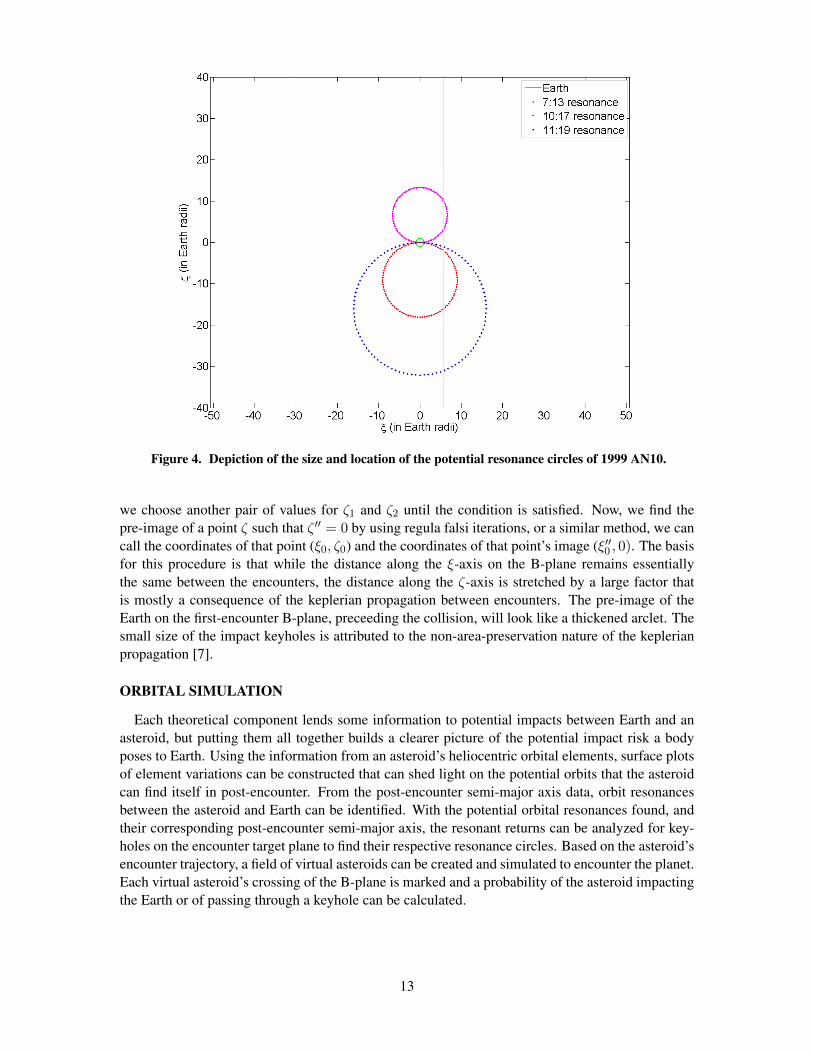
Figure 4. Depiction of the size and location of the potential resonance circles of 1999 AN10.

we choose another pair of values for ζ1 and ζ2 until the condition is satisfied. Now, we find thepre-image of a point ζ such that ζ ′′ = 0 by using regula falsi iterations, or a similar method, we cancall the coordinates of that point (ξ0, ζ0) and the coordinates of that point’s image (ξ′′0 , 0). The basisfor this procedure is that while the distance along the ξ-axis on the B-plane remains essentiallythe same between the encounters, the distance along the ζ-axis is stretched by a large factor thatis mostly a consequence of the keplerian propagation between encounters. The pre-image of theEarth on the first-encounter B-plane, preceeding the collision, will look like a thickened arclet. Thesmall size of the impact keyholes is attributed to the non-area-preservation nature of the keplerianpropagation [7].

ORBITAL SIMULATION

Each theoretical component lends some information to potential impacts between Earth and anasteroid, but putting them all together builds a clearer picture of the potential impact risk a bodyposes to Earth. Using the information from an asteroid’s heliocentric orbital elements, surface plotsof element variations can be constructed that can shed light on the potential orbits that the asteroidcan find itself in post-encounter. From the post-encounter semi-major axis data, orbit resonancesbetween the asteroid and Earth can be identified. With the potential orbital resonances found, andtheir corresponding post-encounter semi-major axis, the resonant returns can be analyzed for key-holes on the encounter target plane to find their respective resonance circles. Based on the asteroid’sencounter trajectory, a field of virtual asteroids can be created and simulated to encounter the planet.Each virtual asteroid’s crossing of the B-plane is marked and a probability of the asteroid impactingthe Earth or of passing through a keyhole can be calculated.

13

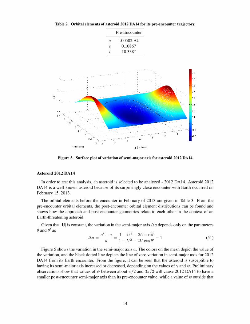
Table 2. Orbital elements of asteroid 2012 DA14 for its pre-encounter trajectory.

Pre-Encounter

a 1.00502 AUe 0.10867i 10.338

Figure 5. Surface plot of variation of semi-major axis for asteroid 2012 DA14.

Asteroid 2012 DA14

In order to test this analysis, an asteroid is selected to be analyzed - 2012 DA14. Asteroid 2012DA14 is a well-known asteroid because of its surprisingly close encounter with Earth occurred onFebruary 15, 2013.

The orbital elements before the encounter in February of 2013 are given in Table 3. From thepre-encounter orbital elements, the post-encounter orbital element distributions can be found andshows how the approach and post-encounter geometries relate to each other in the context of anEarth-threatening asteroid.

Given that |U| is constant, the variation in the semi-major axis ∆a depends only on the parametersθ and θ′ as

∆a =a′ − aa

=1− U2 − 2U cos θ

1− U2 − 2U cos θ′− 1 (51)

Figure 5 shows the variation in the semi-major axis a. The colors on the mesh depict the value ofthe variation, and the black dotted line depicts the line of zero variation in semi-major axis for 2012DA14 from its Earth encounter. From the figure, it can be seen that the asteroid is susceptible tohaving its semi-major axis increased or decreased, depending on the values of γ and ψ. Preliminaryobservations show that values of ψ between about π/2 and 3π/2 will cause 2012 DA14 to have asmaller post-encounter semi-major axis than its pre-encounter value, while a value of ψ outside that

14

Figure 6. Surface plot of variation of inclination for asteroid 2012 DA14.

region will result in a larger semi-major axis after the Earth encounter.

The tangent of inclination is defined as

tan i =cosφ sin θ

1/U + cos θ=

Uz

1 + Uy(52)

and after the rotation of the relative velocity vector by the deflection angle γ in the direction of ψ, itbecomes

tan i′ =cosφ sin θ cos γ − cosφ cos θ sin γ cosψ + sinφ sin γ sinψ

1/U + cos θ cos γ + sin θ sin γ cosψ(53)

The variation in inclination can be described by ∆i = tan i′ − tan i [4]. Figure 6 depicts thevariation of the inclination of the orbits of asteroid 2012 DA14. The black dotted line on the meshedgrid shows the line of zero variation of the inclination after the encounter with the Earth. The plotof the post-encounter inclination variation shows that the assumed inclination of the asteroid afterthe encounter will mostlikely decrease - the question being by how much. There is a small regionof the surface that would result in a small increase in inclination, very small deflection angles andvalues of ψ around π/2.

Recalling thate2 = U4 + 4U2

y + U2x(1− U2 − 2Uy) + 4U2Uy (54)

the expression for the pre-encounter eccentricity of the asteroid orbit can be expressed in terms ofthe relative velocity magnitude and its components. Making a substitution for the correspondingpost-encounter terms, the value of the eccentricity after the encounter with the target planet can becalculated as

e =√U ′4 + 4U ′2y + U ′2x (1− U ′2 − 2U ′y) + 4U ′2U ′y (55)

Taking the difference between the post- and pre-encounter eccentricities shows the variation in theorbital eccentricity (∆e = e′ − e) based on the planetary encounter. Figure 7 depicts the variationof the eccentricity of asteroid 2012 DA14. The black dotted lines shown in the figure indicate

15

Figure 7. Surface plot of variation of eccentricity for asteroid 2012 DA14.

the level of zero variation between the pre- and post-encounter eccentricities of the asteroid. Theplot of eccentricity variation has a bit more complicated structure for this asteroid than semi-majoraxis or inclination, and shows the opposite outcome than the inclination variation - showing a post-encounter eccentricity greater than the pre-encounter value. Asteroid 2012 DA14 would have moreeccentric post-encounter orbits for values of ψ that approach the ends of the feasible domain [0, 2π]and values near π. Values of ψ near π/2 and 3π/2 seem to have a negative effect on the orbitaleccentricities of the body, especially with small or large turning angles.

Before finding the potential orbital resonances that exist for asteroid 2012 DA14 from its en-counter with Earth, it would be helpful to first see what resulting post-encounter orbital parametersfor the asteroid are estimated to be. Using the encounter analysis described in the Post-Encounter

Table 3. Orbital elements of asteroid 2012 DA14 for its post-encounter trajectory.

Post-Encounter

a 0.9108 AUe 0.0888i 11.75

Orbital Trajectory section, the orbital elements of the post-encounter heliocentric orbit are calcu-lated, as shown in Table 3. It can be seen based on the resulting orbital elements that the inclinationof the asteroid is predicted to increase and both the eccentricity and semi-major axis would decrease.These results seem to agree with the variations shown in Figures 5, 6, and 7.

Now that we know the expected post-encounter semi-major axis of 2012 DA14, the potentialorbital resonances can be searched through to find any that the asteroid could fall into. Usinga small two percent error tolerance for the orbital ratio (k/h), 2012 DA14 doesn’t fall into anorbital resonance that would come back to impact the Earth in the next 10 years. There are orbital

16

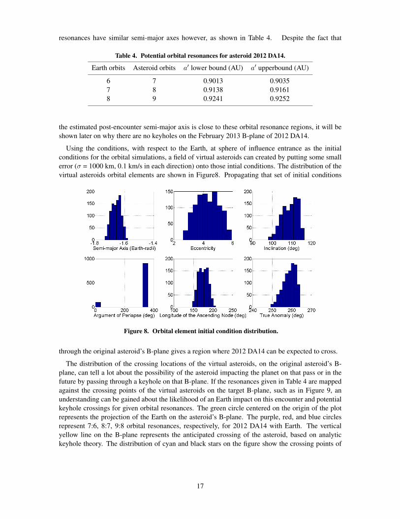
resonances have similar semi-major axes however, as shown in Table 4. Despite the fact that

Table 4. Potential orbital resonances for asteroid 2012 DA14.

Earth orbits Asteroid orbits a′ lower bound (AU) a′ upperbound (AU)

6 7 0.9013 0.90357 8 0.9138 0.91618 9 0.9241 0.9252

the estimated post-encounter semi-major axis is close to these orbital resonance regions, it will beshown later on why there are no keyholes on the February 2013 B-plane of 2012 DA14.

Using the conditions, with respect to the Earth, at sphere of influence entrance as the initialconditions for the orbital simulations, a field of virtual asteroids can created by putting some smallerror (σ = 1000 km, 0.1 km/s in each direction) onto those intial conditions. The distribution of thevirtual asteroids orbital elements are shown in Figure8. Propagating that set of initial conditions

Figure 8. Orbital element initial condition distribution.

through the original asteroid’s B-plane gives a region where 2012 DA14 can be expected to cross.

The distribution of the crossing locations of the virtual asteroids, on the original asteroid’s B-plane, can tell a lot about the possibility of the asteroid impacting the planet on that pass or in thefuture by passing through a keyhole on that B-plane. If the resonances given in Table 4 are mappedagainst the crossing points of the virtual asteroids on the target B-plane, such as in Figure 9, anunderstanding can be gained about the likelihood of an Earth impact on this encounter and potentialkeyhole crossings for given orbital resonances. The green circle centered on the origin of the plotrepresents the projection of the Earth on the asteroid’s B-plane. The purple, red, and blue circlesrepresent 7:6, 8:7, 9:8 orbital resonances, respectively, for 2012 DA14 with Earth. The verticalyellow line on the B-plane represents the anticipated crossing of the asteroid, based on analytickeyhole theory. The distribution of cyan and black stars on the figure show the crossing points of

17

Figure 9. Encounter B-plane for February 2013 encounter of 2012 DA14 with Earth.

the simulated virtual asteroids on the B-plane obtained via numerical integration and state transitionmatrix propagation.

Based on the results, the cluster of crossing locations seem to slightly straddle the anticipatedcrossing line, giving a sense of consistency for the gathered results. As mentioned previously, theshown resonance circles do not intersect the yellow line at any point, implying that no keyhole existson this plane for those particular orbital resonances. Given no resonance circle intersections, focuscan be drawn to the potential of an Earth impact on this encounter, rather than the possibility of akeyhole passage.

IMPACT PROBABILITY COMPUTATION

One of the simplest ways, in theory not necessarily computationally, of calculating an impactprobability of an asteroid and a planet is to simply divide the number of virtual asteroids that hit theplanet, known as virtual impactors, by the total number of virtual asteroids used in the computation.A drawback of this method is that it can be computationally expensive, the number of virtual aster-oids that would need to be used is approximately equal to the inverse of the impact probability [6].Alternative methods of impact probability computation have been developed in the literature by

18

using an impact probability model of the form

IP =

∫ ∫ ∫V⊕

PDF (x, y, z)dxdydz (56)

The use of a statistical approximation can decrease the necessary number of simulations. Todo this, a three-dimensional probability density function (PDF) of the asteroid’s close-approachposition has to be found. So, the impact probability of 2012 DA14 becomes the triple integral ofthe PDF over the volume of the Earth. The expression can be simplified by making use of sphericalcoordinates.

IP =

∫ r⊕

0PDF (r)dr = CDF (r⊕)− CDF (0) (57)

=1

2

[erf

(r⊕ − µσ√

2

)− erf

(0− µσ√

2

)](58)

where CDF denotes the cumulative density function, µ is the mean distance from the Earth, σ isthe standard deviation of the periapse distances from the Earth, and r⊕ is the radius of the Earth.This formulation results in a number between 0 and 1, corresponding to the probability of impact.Having a larger pool of virtual asteroids used in the computation increases the computation time,but should yield a more accurate impact prediction [2].

For the example asteroid given here, 2012 DA14, 1000 virtual asteroids were constructed andsimulated. None of the virtual asteroids simulated hit Earth, so by finding the mean and standarddeviation of their radial distances from Earth the values can be plugged into the statistical impactprobability formulation above and obtain a result. The calculated impact probability for this en-counter case of 2012 DA14 is 0.02%. It is important to note again that the result given here is basedon 1000 simulated virtual asteroids, and the results could be made more accurate by simulatingmore virtual asteroids.

CONCLUSIONS

The results in this paper have been obtained by utilizing the capabilities of various orbital theoryand computational techniques. Through the use of close encounter geometry, the variation in orbitalelements between pre-encounter and post-encounter heliocentric orbits were calculated. Using thoseorbital variations potential orbital resonances between the asteroid and Earth were found. Theconcept of B-plane mapping enabled the construction of the asteroid’s encounter B-plane, whichwas used to ascertain the crossing points of virtual asteroids propagated through the B-plane. Andusing analytic keyhole theory, along with the potential orbital resonances found, the location ofkeyholes on the encounter B-plane could be found. Finally, taking the B-plane crossings data anda statistical model for estimating impact probability, the impact probability of the asteroid wascomputed for the current encounter. The combination of techniques yields a first-cut approximationof impact probability for near-Earth asteroids.

FUTURE WORK

To continue building on this work, an asteroid with an established keyhole property can lendvalidity to the methodology established in this paper. Asteroids such as Apophis and 2013 PDC-E,a fictitious asteroid created as an exercise at the 3rd Planetary Defense Conference in April 2013,

19

have known keyholes on their respective B-planes. With the existence of keyholes on an encounterB-plane comes the possibility of the asteroid passing through those keyholes, so the calculation ofthe probability of a keyhole passage needs to be made. Also, expanding the analysis to take intoaccount multiple successive encounters and finding impact probabilities for encounters far in thefuture would enhance the capabilities of this analysis.

ACKNOWLEDGEMENTS

This research has been supported in part by a NIAC (NASA Innovative Advanced Concepts)Phase 2 study and an Iowa Space Grant Consortium grant.

REFERENCES[1] Chodas, P. W. and Yeomans, D., “Orbit Determination and Estimation of Impact Probability for Near

Earth Objects,” AAS 09-002, AAS/AIAA Space Flight Mechanics Meeting, 2009.[2] Pitz, A., Teubert, C., and Wie, B., “Earth-Impact Probability Computation of Disrupted Asteroid Frag-

ments Using GMAT/STK/CODES,” AAS 11-408, AAS/AIAA Astrodynamics Specialist Conference,Girdwood, AK, August 1-4, 2011.

[3] Yeomans, D. K., Chodas, P. W., Sitarski, G., Szutowicz, S., and Krolikowska, M., “Cometary Orbit Deter-mination and Nongravitational Forces,” Comets II, The Lunar and Planetary Institute, 2004, pp. 137-152.

[4] Carusi, A., Valsecchi, G. B., and Greenberg, R., “Planetary Close Encounters: Geometry of Approachand Post-Encounter Orbital Parameters,” Celestial Mechanics and Dynamical Astronomy, Vol. 49, 1990,pp. 111-131.

[5] “Gravity Assist Interplanetary Trajectories.” Welcome to the Orbital and Celestial Mechanics Website,C. David Eagle, 9 Dec. 2012. Web. 4 Dec. 2013.

[6] Milani, A., Chesley, S. R., Chodas, P. W., and Valsecchi, G. B., “Asteroid Close Approaches: Analysisand Potential Impact Detection,” Asteroids III, The Lunar and Planetary Institute, p. 55-69, 2002.

[7] Valsecchi, G. B., Milani, A., Chodas, P. W., and Chesley, S. R., “Resonant Returns to Close Approaches:Analytic Theory,” Astron. Astrophys., 2001.

[8] Born, George H., “Design of the Approach Trajectory: B-plane Targeting,” ASEN 5519: InterplanetaryMission Design, University of Colorado at Boulder, 2005.

[9] Bourdoux, Arnaud. “Characterisation and Hazard Mitigation of Resonant Returning Near Earth Objects:The Case of 2004 MN,” Diss. Universite De Liege, 2004.

[10] Near-Earth Object Program, Ed. D. Yeomans, National Aeronautics and Space Administration.http://neo.jpl.nasa.gov/index.html.

[11] Yeomans, D., Bhaskaran, S., Chesley, S., Chodas, P., Grebow, D., Landau, D., Petropoulos,A., and Sims, J., “Report on Asteroid 2011 AG5 Hazard Assessment and Contingency Planning.”Near-Earth Object Program. Ed. D. K. Yeomans, National Aeronautics and Space Administration.http://neo.jpl.nasa.gov/index.html.

20