(Preprint) AAS 20-503

MOTION PLANNING AND CONTROL FOR ON-ORBIT ASSEMBLYUSING LQR-RRT* AND NONLINEAR MPC

Bryce Doerr∗ and Richard Linares†

Deploying large, complex space structures is of great interest to the modern scien-tific world as it can provide new capabilities in obtaining scientific, communica-tive, and observational information. However, many theoretical mission designscontain complexities that must be constrained by the requirements of the launchvehicle, such as volume and mass. To mitigate such constraints, the use of on-orbitadditive manufacturing and robotic assembly allows for the flexibility of buildinglarge complex structures including telescopes, space stations, and communica-tion satellites. The contribution of this work is to develop motion planning andcontrol algorithms using the linear quadratic regulator and rapidly-exploring ran-domized trees (LQR-RRT*), path smoothing, and tracking the trajectory using aclosed-loop nonlinear receding horizon control optimizer for a robotic Astrobeefree-flyer. By obtaining controlled trajectories that consider obstacle avoidanceand dynamics of the vehicle and manipulator, the free-flyer rapidly considers andplans the construction of space structures. The approach is a natural generaliza-tion to repairing, refueling, and re-provisioning space structure components whileproviding optimal collision-free trajectories during operation.

INTRODUCTION

On-orbit robotic assembly of large, complex space structures is an emerging area of autonomythat can provide greater access to scientific, communicative, and observational knowledge that isotherwise limited or unknown. When developing space structures, the missions typically have tomeet launch vehicle lifting constraints including volume and mass.1–3 These constraints limit thedesign envelope the structure occupies to conduct its mission. By constructing the structure inspace instead, the volumetric constraints affected by the lifting capacity of the launch vehicle canbe eliminated. On-orbit assembly also provides the capabilities to extend the life or upgrade spacestructure hardware including repairing, refueling, and re-provisioning.2 Thus, it can be more costeffective to repair or refuel a space structure on-orbit than to develop a new mission to replaceit. This in turns allows for flexibility while building large space telescopes, space stations, andcommunication satellites.4

The use of robotic systems to assemble structures has made significant progress for ground-basedapplications, including advances in material deposition and robotic manipulation. For example,geometrically complex components and devices can be produced using improvements in additivemanufacturing.5, 6 With robotic structural assembly, modular control strategies utilizing componentgeometry have been developed to build structures using ground and aerial robotics.7, 8 Multi-robotic

∗Postdoctoral Fellow, Department of Aeronautics and Astronautics, Massachusetts Institute of Technology, 02139.†Charles Stark Draper Assistant Professor, Department of Aeronautics and Astronautics, Massachusetts Institute of Tech-nology, 02139.

1

arX

iv:2

008.

0284

6v1

[cs

.RO

] 6

Aug

202

0

systems have also been designed to collaboratively propel on, manipulate, and transport voxels toconstruct cellular beams, plates, and enclosures9 and by using coarse and fine manipulation tech-niques.10 For larger multi-robotic systems, distributed control has been used so agents collectivelyclimb and assemble the structure they are building on.11 These robotic systems provide technologiesthat envelop the area of constructing large-scale structures, which has direct applications to space.

Ground robotics has also provided technological advancements in motion planning and trajectoryoptimization, which is the foundation necessary to assemble structures. One of these methods isthe Covariant Hamiltonian Optimization for Motion Planning (CHOMP).12 CHOMP is a trajectoryoptimization method that uses gradient techniques to construct trajectories based on the cost, dy-namics, and obstacle constraints from an initial and possibly unfeasible trajectory. However, evenwith gradient information of the state-space, the optimization technique may get stuck in a localminimum, but this method provides a base approach to path planning of on-orbit assembly. Anotherapproach is the Stochastic Trajectory Optimization for Motion Planning (STOMP).13 Similarly toCHOMP, STOMP is a trajectory optimization method that constructs trajectories based on mini-mizing the cost constrained to obstacle avoidance and the dynamics. In this method, no gradientinformation is used, so costs that are non-differentiable and non-smooth can still be used to findoptimal trajectories; however, optimizing trajectories with this technique is inefficient compared toCHOMP since cost function gradient information is not utilized.

A numerically robust and computationally efficient method to trajectory optimization is achievedthrough the use of sequential convex programming (TrajOpt).14 This method uses sequential convexprogramming (SCP) to numerically optimize L1 distance penalties for both inequality and equal-ity constraints. The method solves a convex problem based on approximating the cost and con-straints, which are non-convex using sequential quadratic programming. A computationally simpleralgorithm to SCP is the proximal averaged Newton-type method for optimal control (PANOC) al-gorithm.15 The PANOC optimizer is a line-search method that integrates Newton-type steps andforward-backward iterations over a real-valued continuous merit function. Thus, fast convergenceis enabled using first-order information of the cost function and reduction in linear algebra opera-tions when compared to SCP.15, 16

One final approach to planning dynamically feasible trajectories is using RRT*.17 This is asampled-based algorithm, which produces asymptotically optimal motion planning solutions to adomain-heuristic. Historically, the domain-heuristic has been a Euclidean distance metric to min-imize the L2 distance, but this has been improved to reflect the dynamics and control of systemsusing the cost-to-go pseudo-metric based on the linear quadratic regulator (LQR).18 The advantageof RRT*-based algorithms is that it can be applied to real-time systems in a computationally efficientmanner in which the sampling itself can be interrupted at set time-intervals to allow for real-timeoperation as well as provide collision-free trajectories.

The concept of robotic assembly of space structures is becoming closer to reality with upcomingNASA missions and concepts. The Restore-L servicing mission is an upcoming mission that willrefuel the Landsat 7 spacecraft on-orbit through the use of autonomous rendezvous and graspingtechnology.19 Although specific algorithms on the Restore-L mission are proprietary, a general pa-per submitted by Gaylor discusses innovative algorithms for safe spacecraft proximity operations.20

For this method, it is assumed that the servicer spacecraft and the primary spacecraft are unable tocommunicate with each other, but the servicer spacecraft is able to collect the primary spacecraftstates from a ground station. Trajectory design is implemented using safety ellipses to prevent col-lisions while circumnavigating the primary spacecraft in order to map waypoints for possible injec-

2

tion. This trajectory method allows for safe rendezvous when information of the primary spacecraftis limited, which is useful to robotic assembly since the components are uncommunicative.

Industry and academia have also proposed concepts to advance the field of robotic assemblyof space structures. Tethers Unlimited, Inc. is currently enabling new technologies for on-orbitfabrication including antennas, solar panels, and truss structures using SpiderFab.21 Made In Space,Inc. is also planning on manufacturing and assembly of spacecraft components on-orbit throughits Archinaut One.22 These assemblers are defined by capturing the structure with a robotic armfor servicing or construction. Alternatively, space structures can be assembled using proximityoperations with free-flyer robots.1 At MIT’s Space Systems Laboratory (SSL), Astrobee, a sixdegree of freedom (DOF) free-flyer with a 3 DOF robotic arm, is being used to develop capabilitiesrelating to microgravity manipulation, multi-agent coordination, and higher-level autonomy. Thisresearch will be developed for tests on the International Space Station (ISS).23 Thus, Astrobee hasthe functionality necessary to serve as a testbed for developing modular motion planning strategiesfor on-orbit assembly.

This work builds on these technologies by extending LQR-RRT*, PANOC, obstacle avoidance,and the Astrobee testbed for application of on-orbit robotic assembly of space structures, whichoffers improvements in computational efficiency and optimal collision free trajectories for con-structing next generation telescopes, space stations, and communication satellites.

PROBLEM FORMULATION

In this work, the motion planning and control necessary for on-orbit assembly of space structuresmakes use of LQR-RRT*, a shortcutting trajectory smoothing algorithm, and model predictive con-trol (MPC) using a PANOC nonconvex solver. Specifically, LQR-RRT* is applied to the Astrobeefree-flyer to obtain an initial sub-optimal but collision-free trajectory. Although the trajectory canbe optimized directly to determine the control inputs necessary for the robot, the trajectory may bejerky and unnatural with respect to the target due to the random sampling used in the algorithm.Thus, a trajectory smoothing algorithm using shortcutting is introduced to mitigate the effect ofrandom sampling from the initial trajectory and also considers collision avoidance. Unfortunately,the trajectory obtained through smoothing is not time-dependent, so the smoothed trajectory is re-computed through an LQR control method. With this new trajectory, MPC is applied through aPANOC nonconvex solver to obtain the control inputs to follow this trajectory. Thus, the robot canfollow the planned trajectory to manipulate and assemble parts into structures. The benefit of usinga LQR-RRT* and a trajectory smoother motion planner is the reduction in computational complex-ity of determining optimal solutions through the PANOC nonconvex solver. The state space can becomplex due to the free-flyer dynamics and the increase in obstacles during the on-orbit assemblyprocess, so motion planning and control solutions must continuously be feasible as the complexityincreases in the problem. The control hierarchy for this work is shown in Figure 1, in which thehigh level LQR-RRT* planning has a lower computational bandwidth and larger control abstractionthan its low level MPC counterpart which promotes exploration for finding paths and precision forconverging and maintaining a path. To begin, motion planning and control is presented for a generalnonlinear system.

The continuous time dynamics for a nonlinear system is given by

x(t) = f(x(t),u(t)), (1)

where x(t) ∈ Rnx is the robot state and u(t) ∈ Rnu is the robot control input about time t where nx

3

Figure 1. Motion planning and control hierarchy for the on-orbit assembler.

and nu are the state size and control vector, respectively. The state vector contains the kinematicsand dynamics for both the translational and rotational motion of the robot as well as any manipulatorattached. The control vector contains the forces and torques necessary to actuate the robot. Formotion planning using LQR-RRT* and nonlinear MPC, the dynamics are discretized. Additionallyfor LQR-RRT*, the dynamics must also be linearized to obtain approximate solutions using lineartime-varying (LTV) systems. By discretization and linearization, a linear-time varying system canbe obtained in the form

δxk+1 = Akδxk +Bkδuk, (2)

where Ak and Bk are the state and control matrices at a time-step k. The terms δxk = (xk − xk)and δuk = (uk − uk) are the perturbation state and control about some operating point xk. Forthis work, the operating point occurs at some target xk = xdes. For a discrete nonlinear system, theequation is given by

xk+1 = xk +1

6h(k1 + 2k2 + 2k3 + k4), (3a)

k1 = f(xk,uk), (3b)

k2 = f(xk +k1

2,uk), (3c)

k3 = f(xk +k2

2,uk), (3d)

k4 = f(xk + k3,uk). (3e)

The full derivation of the linearization and discretization using a first-order Taylor series expansionand a fourth-order Runge-Kutta method is presented in the Appendix. The goal is to plan andcontrol a robotic free-flyer for on-orbit assembly constrained to dynamics and obstacles (parts to beassembled) about a quadratic cost function

J(δx0, δU0:N−1) =

N−1∑k=0

l(δxk, δuk) + lN (δxN ), (4)

where δU0:N−1 = [δu0, δu1, · · · , δuN−1] is the control sequence, l(δxk, δuk) is the running cost,

4

and lN (δxN ) is the terminal cost to a time N . This is given by

l(δxk, δuk) =1

2

1δxkδuk

T 0 qTk rTkqk Qk Pkrk Pk Rk

1δxkδuk

, lN (δxN ) =1

2δxTNQNδxN + δxTNqN ,

(5)where qk, rk, Qk, Rk, and Pk are the running weights (coefficients), and QN and qN are theterminal weights. The weight matrices, Qk and Rk, are positive definite and the block matrix[Qk PkPk Rk

]is positive-semidefinite.24

MOTION PLANNING AND CONTROL

LQR-RRT*

The high level motion planning for an on-orbit free-flyer is developed using LQR-RRT*. Themotivation for this work is that it provides computationally efficient, collision-free trajectories in acomplex state-space through sampling.18 Since LQR-RRT* and its algorithms have been discussedextensively in literature,25 an overview of LQR-RRT* is discussed with application to on-orbitassembly using free-flyers. Note that the discussion follows closely to Perez.18

RRT* : For a nonlinear system given in Eq. (1), the goal is to obtain a trajectory that minimizesthe cost function given in Eq. (4) with an initial state x0 and goal state xdes. By using RRT*, adynamically feasible continuous trajectory with the property of asymptotic optimality can be found.RRT* consists of five major components. This includes:

• Random sampling: The state-space is randomly sampled uniformly to obtain a node (state).This is called xrand.

• Near nodes: With a current set of nodes N in the tree and the xrand, a subset of Nnear ⊆ N isfound close to xrand using a distance metric,{

x′ ∈ N : ||xrand − x′|| ≤ γ(

lognn

)1/nx}, (6)

where n is the number of nodes in the tree, γ is a constant, and || · || is a distance metric.

• Choosing a parent: Minimal cost trajectories for each candidate node in Nnear is computedwith respect to xrand. This is through a straight line steering method. The node with thelowest cost (xmin) becomes the parent of the random node and a trajectory σmin is returned.

• Collision checking: The path σmin is checked against any obstacles within the state-space.Specifics to collision checking is discussed in the Collision Avoidance Section.

• Rewire: If the path σmin and node xrand is collision-free, xrand is added to the set of nodesN, and then attempts to reconnect xrand with the set Nnear if the cost is less than its currentparent node.

These algorithm components provide a recursion to obtaining asymptotically optimal trajectories.Careful design of distance heuristics must be considered for complex problems. However, ex-tensions of this initial algorithm can be made by minimizing an LQR cost and computing LQRtrajectories between nodes instead.

5

LQR : Although the initial free-flyer dynamics is nonlinear given in Eq. (1), a linearized anddiscretized approximation can be obtained as a LTV system in Eq. (2). The quadratic cost given byEq. (4) can be simplified to

J(δx0, δU0:N−1) =N−1∑k=0

δxTk qk + δuTk rk +1

2δxTkQkδxk +

1

2δuTkRkδuk + δuTk Pkδxk

+1

2δxTNQNδxN + δxTNqN .

(7)

The optimal control solution is based on minimizing the cost function in terms of the control se-quence which is given by

δU?0:N−1(δx0) = arg minδU0:N−1

J(δx0, δU0:N−1). (8)

To solve for the optimal control solution given by Eq. (8), a value iteration method is used. Valueiteration is a method that determines the optimal cost-to-go (value) starting at the final time-stepand moving backwards in time minimizing the control sequence. Similar to Eq. (4) and (8), thecost-to-go and optimal cost-to-go are defined as

J(δxk, δUk:N−1) =N−1∑k

l(δxk, δuk) + lN (δxN ), (9a)

V (δxk) = minδUk:N−1

J(δxk, δUk:N−1), (9b)

Instead, the cost starts from time-step k instead of k = 0. At a time-step k, the optimal cost-to-gofunction is a quadratic function given by

V (δxk) =1

2δxTk Skδxk + δxTk sk + ck, (10)

where Sk, sk, and ck are computed backwards in time using the value iteration method. First, thefinal conditions SN = QN , sN = qN , and cN = c are set. This reduces the minimization ofthe entire control sequence to just a minimization over a control input at a time-step which is theprinciple of optimality.26 To find the optimal cost-to-go, the Riccati equations are used to propagatethe final conditions backwards in time given by

Sk = ATk Sk+1Ak +Qk −(BTk Sk+1Ak + P Tk

)T (BTk Sk+1Bk +Rk

)−1 (BTk Sk+1Ak + P Tk

),

(11a)

sk = qk +ATk sk+1 +ATk Sk+1gk

−(BTk Sk+1Ak + P Tk

)T (BTk Sk+1Bk +Rk

)−1 (BTk Sk+1gk +BT

k sk+1 + rk),

(11b)

ck = gTk Sk+1gk + 2sTk+1gk + ck+1

−(BTk Sk+1gk +BT

k sk+1 + rk)T (

BTk Sk+1Bk +Rk

)−1 (BTk Sk+1gk +BT

k sk+1 + rk).

(11c)

Using the Ricatti solution, the optimal control policy is in the affine form

δuk(xk) = Kkδxk + lk, (12)

6

where the controller, Kk, and controller offset is given by

Kk = −(Rk +BTk Sk+1Bk)

−1(BTk Sk+1Ak + P Tk ), (13a)

lk = −(Rk +BTk Sk+1Bk)

−1(BTk Sk+1gk +BT

k sk+1 + rk). (13b)

This optimal solution to the LQR problem works for linear approximations of nonlinear equationsof motion and quadratic cost functions, and can be combined directly with RRT* to explore thestate-space and obtain asymptotically optimal, collision-free trajectories.

LQR-RRT* : By incorporating the LQR algorithm with RRT*, the distance heuristic becomesthe quadratic LQR formulation. This algorithm consists of seven major components including:

• Random sampling: This component remains unchanged from RRT*. The state-space is ran-domly sampled uniformly to obtain a node called xrand shown in Fig. 2(a).

• Nearest node: With a current set of nodes N in the tree and xrand, the nearest node in the treeis obtained relative to xrand using the LQR optimal cost-to-go function in Eq. (10) whichsimplifies to

xnearest = arg minx′∈N

(x′ − xrand)TSrand(x

′ − xrand) + (x′ − xrand)srand + crand, (14)

where Srand, srand, and crand are computed about the time-step which xrand occurs. This isshown in Fig. 2(b).

• LQR steer: With xnearest and xrand, a trajectory is obtained using LQR that connects bothnodes. Note that the path obtained can be trajectories that move towards xrand. The finalstate of this path is xnew which appears in Fig. 2(c).

• Near nodes: With the set N and xnew, a subset of Nnear ⊆ N is found close to xnew using theEq. (10) distance metric expressed as{

x′ ∈ N : (x′ − xnew)TSnew(x′ − xnew) + (x′ − xnew)snew + cnew ≤ γ(

lognn

)1/nx}.

(15)This is visualized in Fig. 2(d).

• Choosing a parent: This component is similar to RRT*. Minimal cost trajectories for eachcandidate in Nnear are found with respect to xnew. Instead of the straight line steering methodused in RRT*, the LQR steering is used instead to obtain the node with the lowest cost (xmin)and the trajectory σmin. This becomes the parent node of xnew which is shown in Fig. 2(e).

• Collision checking: This component remains unchanged from RRT* and is discussed in theCollision Avoidance Section. A visualization is made in Fig. 2(f).

• Rewire near nodes: This component is similar to RRT*. If the path σmin and node xnew iscollision-free, xnew is added to the set of nodes N, and then attempts to reconnect xnew withthe set Nnear if the cost is less than its current parent node using LQR steering. The processof rewiring the nodes is depicted by Fig. 2(g) which results in the trajectory in Fig 2(h).

7

This algorithm provides the recursion to obtain asymptotically optimal trajectories using the LQRdistance heuristic. A single pass of the algorithm is provided in Fig. 2 showing how a trajectoryis built from samples. LQR-RRT* provides an initial trajectory to meet on-orbit assembly goalslike avoiding structural parts used for assembly and providing efficient trajectories to initialize ma-nipulation. Unfortunately, due to the process of sampling through LQR-RRT*, the trajectory maybe jerky and unnatural if not enough samples are taken. Thus, a trajectory smoothing agorithmthrough shortcutting is applied to mitigate this effect as well as consider collision avoidance. Thisis discussed next.

(a) Random Sampling (b) Nearest Node (c) LQR Steer

(d) Near Nodes (e) Choosing a Parent (f) Collision Checking

(g) Rewire Near Nodes (h) Rewired Tree

Figure 2. LQR-RRT* algorithm components.

8

Trajectory Smoothing by Shortcutting

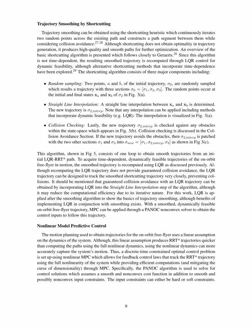
Trajectory smoothing can be obtained using the shortcutting heuristic which continuously iteratestwo random points across the existing path and constructs a path segment between them whileconsidering collision avoidance.27, 28 Although shortcutting does not obtain optimality in trajectorygeneration, it produces high-quality and smooth paths for further optimization. An overview of thebasic shortcutting algorithm is presented which follows closely to Geraerts.28 Since this algorithmis not time-dependent, the resulting smoothed trajectory is recomputed through LQR control fordynamic feasibility, although alternative shortcutting methods that incorporate time-dependencehave been explored.29 The shortcutting algorithm consists of three major components including:

• Random sampling: Two points, a and b, of the initial trajectory, σ0, are randomly sampledwhich results a trajectory with three sections σ0 = [σ1, σ2, σ3]. The random points occur atthe initial and final states xa and xb of σ2 in Fig. 3(a).

• Straight Line Interpolation: A straight line interpolation between xa and xb is determined.The new trajectory is σ2,interp. Note that any interpolation can be applied including methodsthat incorporate dynamic feasibility (e.g. LQR). The interpolation is visualized in Fig. 3(a).

• Collision Checking: Lastly, the new trajectory σ2,interp is checked against any obstacleswithin the state-space which appears in Fig. 3(b). Collision checking is discussed in the Col-lision Avoidance Section. If the new trajectory avoids the obstacles, then σ2,interp is patchedwith the two other sections σ1 and σ3 into σnew = [σ1, σ2,interp, σ3] as shown in Fig 3(c).

This algorithm, shown in Fig 3, consists of one loop to obtain smooth trajectories from an ini-tial LQR-RRT* path. To acquire time-dependent, dynamically feasible trajectories of the on-orbitfree-flyer in motion, the smoothed trajectory is recomputed using LQR as discussed previously. Al-though recomputing the LQR trajectory does not provide guaranteed collision avoidance, the LQRtrajectory can be designed to track the smoothed shortcutting trajectory very closely, preventing col-lisions. It should be mentioned that guaranteed collision avoidance with an LQR trajectory can beobtained by incorporating LQR into the Straight Line Interpolation step of the algorithm, althoughit may reduce the computational efficiency due to its iterative nature. For this work, LQR is ap-plied after the smoothing algorithm to show the basics of trajectory smoothing, although benefits ofimplementing LQR in conjunction with smoothing exists. With a smoothed, dynamically feasibleon-orbit free-flyer trajectory, MPC can be applied through a PANOC nonconvex solver to obtain thecontrol inputs to follow this trajectory.

Nonlinear Model Predictive Control

The motion planning used to obtain trajectories for the on-orbit free-flyer uses a linear assumptionon the dynamics of the system. Although, this linear assumption produces RRT* trajectories quickerthan computing the paths using the full nonlinear dynamics, using the nonlinear dynamics can moreaccurately capture the system’s motion. Thus, a discrete-time constrained optimal control problemis set up using nonlinear MPC which allows for feedback control laws that track the RRT* trajectoryusing the full nonlinearity of the system while providing efficient computations (and mitigating thecurse of dimensionality) through MPC. Specifically, the PANOC algorithm is used to solve forcontrol solutions which assumes a smooth and nonconvex cost function in addition to smooth andpossibly nonconvex input constraints. The input constraints can either be hard or soft constraints.

9

(a) Random Sampling & Straight LineInterpolation

(b) Collision Checking (c) Rewired Trajectory

Figure 3. Trajectory smoothing using the shortcutting heuristic.

In this section, a single-shooting formulation of the optimal control problem is presented usingPANOC. Note that the discussion follows closely to Sopasakis.30

A general parametric optimization problem is given by

minυ∈Υ

f(υ, p), (16a)

Subject to :F1(υ, p) ∈ C, (16b)

F2(υ, p) = 0, (16c)

where υ ∈ Rnυ is the decision variable vector, p ∈ Rnp is the parameter vector, f(υ, p) : Rn0 → Ris a continuously differentiable (and possibly nonconvex) function with a Lf -Lipschitz gradient,Υ ⊆ Rn0 is a nonempty, closed set for computing projects, F1(υ, p) : Rn0 → Rn1 is a smoothmapping with a Lipschitz-continuous Jacobian bounded on U , C ⊆ Rn1 is a convex set to deter-mine distances, and F2(υ, p) : Rn0 → Rn2 is a function in which ||F2(υ, p)||2 is continuouslydifferentiable with a Lipschitz-continuous gradient.

The constraints given by Eqs. (16b) and (16c) are accounted in the optimization using the aug-mented Lagrangian method and the penalty method, respectively. Equality and inequality con-straints are given by

Heq(υ, p) = 0, (17a)

Hineq(υ, p) ≤ 0, (17b)

and both can be included into Eqs. (16b) and (16c). By letting F1(υ, p) = Heq(υ, p) in Eq. (16b),the equality is incorporated by setting C = 0. The inequality constraint can be included in Eq. (16b)by letting F1(υ, p) = Hineq(υ, p) and setting C = {ν ∈ Rn1 : ν ≤ 0}. For Eq. (16c), the equalityconstraint can be found by letting F2(υ, p) = Heq(υ, p) instead. The inequality constraint can beobtained in Eq. (16c) by letting F2(υ, p) = max [0, Hineq(υ, p)].

From the general parametric optimization problem given in Eq. (16), a discrete-time single-shooting optimization problem can be formed as

minU0:N−1

N−1∑k=0

l(Fk(U0:k,x0),uk) + lN (FN (U0:N−1,x0)) (18a)

10

Subject to :uk ∈ U0:N−1, (18b)

F0(u0,x0) = x0, (18c)

Fk+1(U0:k,x0) = f(Fk(U0:k,x0),uk), (18d)

Hk(Fk(U0:k,x0),uk) ≤ 0, (18e)

where Fk(U0:k,x0) is a sequence of functions to obtain xk, f(·,uk) is a nonlinear dynamics func-tion given by Eq. (3), and Hk(Fk(U0:k,x0),uk) are the inequality constraints that can be formed aseither Eq. (16b) or (16c). For a time-step k, the nonlinear MPC formulation can directly be derivedfrom Eq. (18) by optimizing over a prediction horizon Np given by

minUk:(k+Np−1)

Np−1∑j=0

l(Fk+j(U0:(k+j),x0),uk+j) + lNp(FNp(U0:(Np−1),x0)) (19a)

Subject to :uk+j ∈ Uk:(k+Np−1), (19b)

F0(u0,x0) = x0, (19c)

Fk+j+1(U0:(k+j),x0) = f(Fk+j(U0:(k+j),x0),uk+j), (19d)

Hk+j(Fk+j(U0:(k+j),x0),uk+j) ≤ 0. (19e)

At each time-step k, an optimal control sequence of U?k:(k+Np−1) =[u?k,u

?k+1, . . . ,u

?k+Np−1

]is

found, and the first control input, u?k, is applied to the robotic system (Eq. (3)). The predictionhorizon, Np, can be modified to to trade-off the computational performance of the optimization andthe optimality of the solution with respect to the finite horizon N . With the optimization prob-lem formed, the optimal control solutions can be obtained using the PANOC solver to guaranteereal-time performance.15, 30 In the next two sections, the obstacle avoidance constraints and the dy-namical constraints are discussed, which are applied to either the LQR-RRT*, trajectory smoothing,or nonlinear MPC in specific forms.

COLLISION AVOIDANCE

For on-orbit assembly, obstacle avoidance is an area to consider to prevent harm to either the on-orbit free-flyer or the assembled structure. Fortunately, collision avoidance can be implemented inall parts of the problem described in Fig. 1. A component of LQR-RRT* and trajectory smoothingvia shortcutting include a collision checking element which checks whether the path between twonodes intersects with an obstacle. If there is such an intersection, the path between the two nodes isthrown out. The LQR planning algorithm applied after the smoothing does not guarantee collisionavoidance, but the motion planning can be designed to follow the shortcutting trajectory to preventobstacle collisions. Also as discussed previously, the LQR motion planning can be incorporatedinto the Straight Line Interpolation step of the shortcutting algorithm to provide time-dependenttrajectories with guaranteed collision avoidance. Lastly, collision avoidance can be implementeddirectly as a constraint for the nonlinear MPC problem. By solving the nonlinear MPC problemusing a PANOC solver, control solutions can be found that follows a trajectory while avoidingobstacles.

For the on-orbit free-flyer, the goal is to avoid obstacle collisions with structural parts during itsstructural assembly. The obstacles themselves can be tracked by the on-orbit free-flyer or remotelyby another spacecraft or a ground station. By knowing the states of the obstacles, the on-orbitfree-flyer can approximate a keep-out zone using a 3D ellipsoid.31

11

Ellipsoid Method

A 3D ellipsoid constraint bounds an obstacle by an ellipsoidal keep-out zone. If the obstaclehas no uncertainty in its size, an ellipsoid can be formed which encloses the obstacle’s volume. Ifuncertainty in the obstacle’s size exists, the ellipsoid that encloses the obstacles may include a safetyfactor. For estimation problems with assumed Gaussian noise, the corresponding covariance can bedirectly incorporated into the ellipsoid model to represent the uncertainty of the obstacle inside of it.The ellipsoid representation of obstacles can also be directly applied to higher fidelity applications.Instead of bounding a entire space structure with an ellipsoid, individual structural parts can bemodeled with an ellipsoid to be avoided. This is useful for on-orbit assembly applications, sinceindividual structural parts are manipulated in order to assemble larger structures. The ellipsoidalconstraint for collision avoidance is given by

(xpos − xobs)T Pobs (xpos − xobs) ≥ 1, (20)

where xobs is the ellipsoid’s centroid position, Pobs is a positive definite shape matrix of the ellip-soid, and xpos is the position of a point on the path in question. This constraint is nonlinear andnonconvex, but motion planning and control discussed in the previous section are able to handlesuch constraints. If xpos lies outside the ellipsoid, the constraint in Eq. (20) is met (returned true),and if xpos lie inside the ellipsoid, the constraint in Eq. (20) is not met (returned false). Each pointon the trajectory must be evaluated against Eq. (20) to determine whether any collisions occurred.For LQR-RRT* and trajectory smoothing using shortcutting, this is a simple for-loop. For nonlinearMPC, the constraint must be formed as Eq. (17b) given by

Hineq =

1...1

N×1

− diag{X TPobsX} ≤

0...0

N×1

(21)

whereN is the time horizon of the trajectory, X is a stacked sequence of position states specified byX = [(xpos,0 − xobs,0) , (xpos,1 − xobs,1) , . . . , (xpos,N − xobs,N )] ∈ R3×N , and diag(·) transformsthe diagonals of theN×N matrix into a column vector. Note that xobs can be dynamically moving,and thus, a time dependency is included in Eq. (21). This provides the collision check or constraintfor a single obstacle, but this constraint can be expanded to multiple obstacles by comparing thetrajectory position state to every obstacle on the field. This is given by

Hineq =

1...1

(N ·Nobs)×1

−

diag{X TPobs,1X}...

diag{X TPobs,NobsX}

≤0

...0

(N ·Nobs)×1

(22)

where Nobs is the number of obstacles on the field. Thus, obstacle avoidance using the ellipsoidalmethod can be applied to LQR-RRT*, trajectory smoothing using shortcutting, and nonlinear MPCusing PANOC optimization.

Since, Eq. (20) is a nonconvex problem, considerations must be discussed with ill-posed plan-ning problems. If the velocity of the robot is considerably fast, the time update between states ina discrete system can jump a great deal if the time interval is not fine enough. If this distance be-tween two consecutive states is larger than the smallest characteristic length of the ellipsoid, thenoptimization solutions can be found which meet the constraints, but the robot technically collides

12

with the obstacle. Great care must be taken to prevent these ill-posed problems, and one method tomitigate them is by increasing the resolution of the sample time and interpolating the trajectory inthe obstacle constraint comparison.32 Therefore, collision-free trajectories can be obtained from theoptimization solutions.

ROBOTIC FREE-FLYER DYNAMICS

To show the viability of the motion planning and control of an on-orbit free-flyer for assembly,a multi-rigid body system is used to describe the dynamics. The dynamics are used directly inmotion planning and control of the spacecraft by computing the corresponding linearization anddiscretization discussed in the Appendix.

Multi-Rigid Body Dynamics

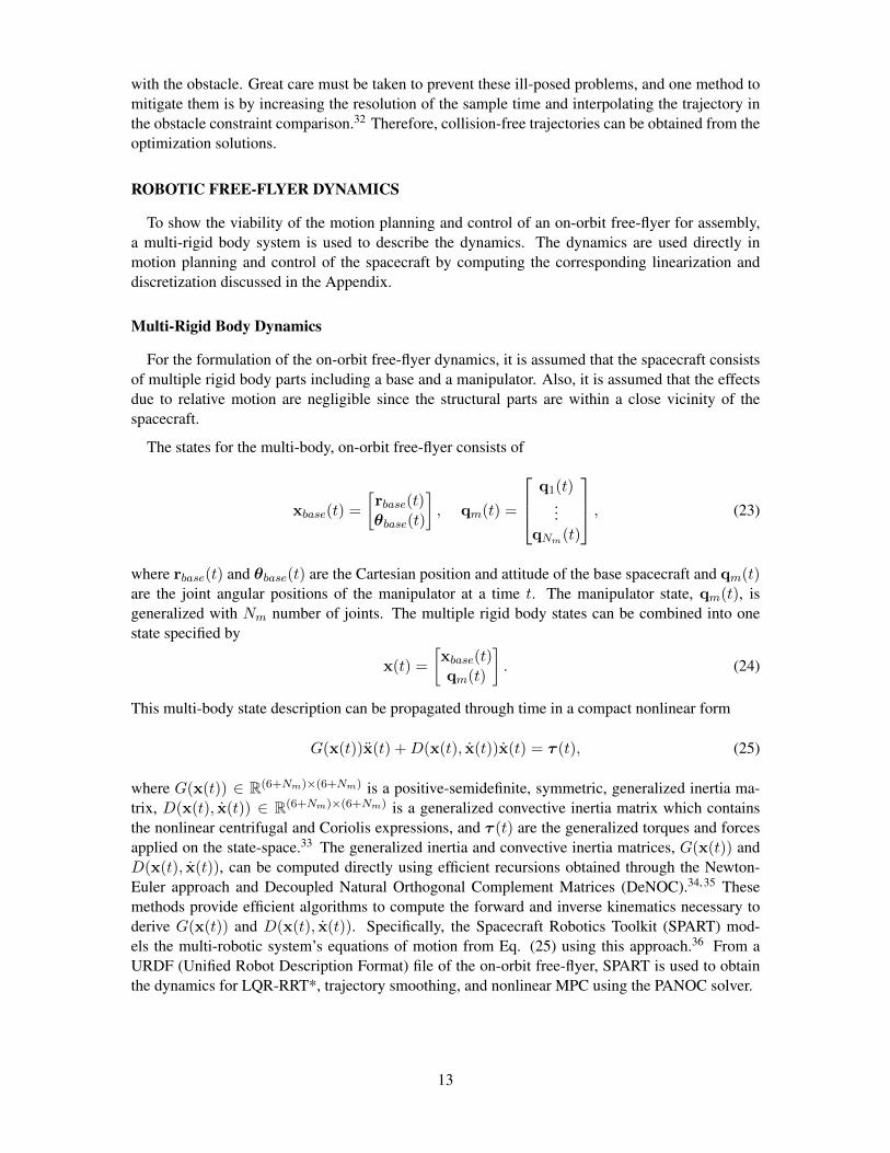
For the formulation of the on-orbit free-flyer dynamics, it is assumed that the spacecraft consistsof multiple rigid body parts including a base and a manipulator. Also, it is assumed that the effectsdue to relative motion are negligible since the structural parts are within a close vicinity of thespacecraft.

The states for the multi-body, on-orbit free-flyer consists of

xbase(t) =

[rbase(t)θbase(t)

], qm(t) =

q1(t)...

qNm(t)

, (23)

where rbase(t) and θbase(t) are the Cartesian position and attitude of the base spacecraft and qm(t)are the joint angular positions of the manipulator at a time t. The manipulator state, qm(t), isgeneralized with Nm number of joints. The multiple rigid body states can be combined into onestate specified by

x(t) =

[xbase(t)qm(t)

]. (24)

This multi-body state description can be propagated through time in a compact nonlinear form

G(x(t))x(t) +D(x(t), x(t))x(t) = τ (t), (25)

where G(x(t)) ∈ R(6+Nm)×(6+Nm) is a positive-semidefinite, symmetric, generalized inertia ma-trix, D(x(t), x(t)) ∈ R(6+Nm)×(6+Nm) is a generalized convective inertia matrix which containsthe nonlinear centrifugal and Coriolis expressions, and τ (t) are the generalized torques and forcesapplied on the state-space.33 The generalized inertia and convective inertia matrices, G(x(t)) andD(x(t), x(t)), can be computed directly using efficient recursions obtained through the Newton-Euler approach and Decoupled Natural Orthogonal Complement Matrices (DeNOC).34, 35 Thesemethods provide efficient algorithms to compute the forward and inverse kinematics necessary toderive G(x(t)) and D(x(t), x(t)). Specifically, the Spacecraft Robotics Toolkit (SPART) mod-els the multi-robotic system’s equations of motion from Eq. (25) using this approach.36 From aURDF (Unified Robot Description Format) file of the on-orbit free-flyer, SPART is used to obtainthe dynamics for LQR-RRT*, trajectory smoothing, and nonlinear MPC using the PANOC solver.

13

SIMULATION RESULTS

For this work, the Astrobee on-orbit free-flyer, with a simplified 2-Degree of Freedom (DOF)manipulator, is tasked for on-orbit assembly of space structures. This includes the motion planningto and from a 3D printer (in which parts are manufactured) and the area which the space structure isbuilt. One top of the simplified manipulator, it is also assumed that the actuation is not constrainedto any limits, and during the manipulation, the mass properties do not change between the combinedAstrobee and structural part.

Table 1. Astrobee: Inertial Properties

Properties Mass [kg] Moment of Inertia [kg m2]Ixx Iyy Izz

Base 7.0 0.11 0.11 0.11Arm 1 1.0 0.05 0.05 0.05Arm 2 1.0 0.05 0.05 0.05End-Effector 4.0 0 0 0

The base Astrobee has a full (6-DOF) capability inside the state-space environment and the ma-nipulator has an additional 2-DOF arm (Nm = 2) from actuation of the joints.37 The mass propertiesfor a simulated Astrobee used in this problem are given in Table 1.37 Note that the properties aremodified for this problem (e.g. the end-effector is assumed to have a mass of 4kg as considerationfor any structural parts attached). From these properties, A URDF robotic description file of As-trobee was designed to obtain the multi-body dynamics necessary for motion planning and controlusing the hierarchy in Fig. 1. The results obtained through this hierarchy are discussed next.

(a) Base Translational States (b) Base Attitude

Figure 4. Translational and attitude states for the base Astrobee using LQR-RRT*(blue) and trajectory smoothing (red).

LQR-RRT*, Trajectory Smoothing, and LQR

In order to assemble structures from 3D printed parts on-orbit, a simulation using LQR-RRT*was developed. For this scenario in Fig. 1, the goal is to find an initial path from Astrobee’s current

14

position to the 3D printer or to the desired location for construction. The trajectories obtained fromLQR-RRT* are shown in blue in Figure 4. The trajectories were found to move between the 3Dprinter and the desired location for construction while avoiding ellipsoidal obstacles. At specificpoints along the path, the trajectory is jerky and unnatural since the algorithm is ran until an initialtrajectory, which completes the path between Astrobee and the desired state, is found. If the LQR-RRT* algorithm continues sampling the space through time, the trajectories obtained would reachasymptotic optimality with respect to the cost function, but for this work, computational efficiencyis necessary for Astrobee to perform on-orbit assembly.

(a) Base Translational States (b) Base Attitude

Figure 5. Translational and attitude states for the base Astrobee using LQR (green)and the reference smoothing trajectory(red).

To mitigate the randomness of sampling in LQR-RRT*, trajectory smoothing by shortcuttingis implemented as shown in red within Figure 4. Specifically, smoother, collision-free paths (inposition and orientation) are found for Astrobee, and mitigation of the randomness of the samplingfrom LQR-RRT* can be observed. As a note from the figure, each point of the shortcutting trajectoryis time independent. This trajectory was projected onto the LQR-RRT* trajectory to show thedifferences between the two trajectories.

Since the smoothed trajectory is time-independent, the smoothed trajectory was recomputed usingLQR which appears in Figure 5 where the green and red lines are the LQR and shortcut trajectories,respectively. In this case, the smoothed trajectory is some desired state the Astrobee must achieve byLQR tracking. From the figure, the response reaches the desired state with a settling time of 3.40s.By using LQR-RRT*, trajectory smoothing, and LQR to obtain a on-orbit Astrobee trajectory, MPCthrough PANOC can be applied to control the spacecraft along this trajectory as well as manipulateparts for on-orbit assembly.

Nonlinear MPC using PANOC

The trajectory obtained from LQR-RRT*, trajectory smoothing, and LQR was applied directlyto the states of the base Astrobee. No trajectories were formed for the Astrobee manipulator dur-ing motion planning. Instead, the manipulator was commanded directly to a desired state usingNonlinear MPC. This is in addition to controlling the base Astrobee through the planned trajectory.The time-history response for the base and manipulator states of the Astrobee free-flyer during the

15

(a) Base Translational States (b) Base Attitude

(c) Manipulator States

Figure 6. Translational and attitude states for the base Astrobee and angular positionstates for the manipulator using nonlinear MPC.

on-orbit assembly is shown in Figure 6. From the figure, the manipulator was commanded to π4 rad

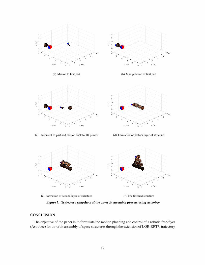
or 0 rad to grasp the structural part or to retract during motion. The nonlinear MPC solver useda prediction horizon, Np, of 10 time-steps into the future with an average of 30ms computationaltime to solve for the control input, thus providing real-time capabilities. Trajectory snapshots for theon-orbit assembly process is shown in Figure 7. The goal for Astrobee is to construct a pyramid-likestructure with 10 ellipsoids constructed from a 3D printer (cube). Figure 7(a) shows Astrobee mov-ing toward the first structural part. In Figure 7(b), Astrobee grasps the first part and starts its motionto the assembly area. Next in Figure 7(c), Astrobee places the first part in its desired area, andAstrobee moves onward to the second part. Figure 7(d) shows the bottom of the structure formed.Figure 7(e) shows the second layer of the structure formed. Figure 7(f) shows the finished pyramid-like structure formed from the ellipsoid structural part. When computing collision avoidance forthe 3D printer and the structural parts, the Pobs in Eq. (20) was designed with a safety factor dueto the size of the Astrobee from its centroid and trajectories obtained from LQR. Thus, control ofcollision-free trajectories for the on-orbit assembly system was obtained.

16

(a) Motion to first part (b) Manipulation of first part

(c) Placement of part and motion back to 3D printer (d) Formation of bottom layer of structure

(e) Formation of second layer of structure (f) The finished structure

Figure 7. Trajectory snapshots of the on-orbit assembly process using Astrobee

CONCLUSION

The objective of the paper is to formulate the motion planning and control of a robotic free-flyer(Astrobee) for on-orbit assembly of space structures through the extension of LQR-RRT*, trajectory

17

smoothing, obstacle avoidance, and nonlinear MPC using PANOC. By setting up a problem in whichparts manufactured by a 3D printer are described by an ellipsoid, collision-free trajectories are foundfor the on-orbit free-flyer. Then, real-time nonlinear MPC solutions were determined to maintaina collision-free optimal trajectory following the 8-DOF free-flyer and manipulator dynamics. Thisprovides the on-orbit free-flyer the ability for on-orbit manipulation and the rapid considerationfor the construction of space structures in simulation. For future work, the goal is to extend thiswork to physical experiments with the Astrobee robot on the ISS, identify changes in moment ofinertia during manipulation, characterize contact during the manipulation, and improve trajectorysmoothing by finding time-dependent solutions.

ACKNOWLEDGMENT

This research was supported by an appointment to the Intelligence Community Postdoctoral Re-search Fellowship Program at Massachusetts Institute of Technology, administered by Oak RidgeInstitute for Science and Education through an interagency agreement between the U.S. Departmentof Energy and the Office of the Director of National Intelligence. The authors wish to acknowledgeuseful conversations related to motion planning and optimization with Keenan Albee, a Ph.D. stu-dent, at the Massachusetts Institute of Technology.

APPENDIX: LINEARIZATION AND DISCRETIZATION

Linearization

The dynamics for a free-flyer robot is described by the nonlinear equations of motion given byEq. (1). In order to apply LQR-RRT*, the equations of motion must be linearized and discretized.By taking a first-order Taylor series expansion of Eq. (1) around an operating point for linearization,x(t) and u(t), a linear time-varying (LTV) system can be found which approximates the nonlinearequation given by

x(t) ≈ f(x(t),u(t))|x(t),u(t) + ∂f(x(t),u(t))∂x(t)

∣∣∣x(t),u(t)

(x(t)− x(t)) + ∂f(x(t),u(t))∂u(t)

∣∣∣x(t),u(t)

(u(t)− u(t)) .

(26)This equation is simplified to a linear state-space model using perturbations from the operating pointgiven by

δx(t) = A(t)δx(t) + B(t)δu(t), (27)

where δx(t) = x(t)− f(x(t),u(t))|x(t),u(t), δx(t) = x(t)− x(t), and δu(t) = u(t)− u(t). BothA(t) and B(t) are time-dependent Jacobians of the nonlinear function f(x(t),u(t)) with respect tox(t) and u(t).

Discretization

Either the full nonlinear dynamics given by Eq. (1) or the approximate linear dynamics given byEq. (27) can be discretized using a fourth-order Runge-Kutta method with a zero-order hold on thecontrol input uk.38 A fourth-order Runge-Kutta integration for Eq. (27) is given by

δxk+1 = δxk +1

6h(k1 + 2k2 + 2k3 + k4). (28)

18

Note that the variable k is the discretized time-step and h is the step size for the system. With thezero-order hold on a control input uk, the k1, k2, k3, and k4 are given by

k1 = Akδxk + Bkδuk

k2 = Ak (δxk + k1/2) + Bkδuk

k3 = Ak (δxk + k2/2) + Bkδuk

k4 = Ak (δxk + k3) + Bkδuk.

(29)

By substituting Eq. (29) into Eq. (28), the discretized system from a fourth-order Runge-Kutta witha zero-order hold on control is

δxk+1 =

(I + hAk +

h2

2!A2k +

h3

3!A3k +

h4

4!A4k

)δxk +

(h+

h2

2!Ak +

h3

3!A2k +

h4

4!A3k

)Bkδuk,

(30)which follows the form of Eq. (2). This discrete, linear approximation for Eq. (1) is used to producetrajectories using LQR-RRT*. Similarly, the a discrete, nonlinear form of Eq. (1) can be obtainedfor nonlinear MPC using the same fourth-order Runge-Kutta method which results in Eq. (3).

REFERENCES[1] C. Jewison, D. Sternberg, B. McCarthy, D. W. Miller, and A. Saenz-Otero, “Definition and testing of an

architectural tradespace for on-orbit assemblers and servicers,” 2014.[2] J. H. Saleh, E. S. Lamassoure, D. E. Hastings, and D. J. Newman, “Flexibility and the value of on-orbit

servicing: New customer-centric perspective,” Journal of Spacecraft and Rockets, Vol. 40, No. 2, 2003,pp. 279–291.

[3] D. Izzo, L. Pettazzi, and M. Ayre, “Mission concept for autonomous on orbit assembly of a largereflector in space,” 56th International Astronautical Congress, Vol. 5, Citeseer, 2005.

[4] W. Doggett, “Robotic assembly of truss structures for space systems and future research plans,” Pro-ceedings, IEEE Aerospace Conference, Vol. 7, IEEE, 2002, pp. 7–7.

[5] D. W. Rosen, “Computer-aided design for additive manufacturing of cellular structures,” Computer-Aided Design and Applications, Vol. 4, No. 5, 2007, pp. 585–594.

[6] T. A. Schaedler and W. B. Carter, “Architected cellular materials,” Annual Review of Materials Re-search, Vol. 46, 2016, pp. 187–210.

[7] K. H. Petersen, R. Nagpal, and J. K. Werfel, “Termes: An autonomous robotic system for three-dimensional collective construction,” Robotics: science and systems VII, 2011.

[8] J. Willmann, F. Augugliaro, T. Cadalbert, R. D’Andrea, F. Gramazio, and M. Kohler, “Aerial roboticconstruction towards a new field of architectural research,” International journal of architectural com-puting, Vol. 10, No. 3, 2012, pp. 439–459.

[9] B. Jenett, A. Abdel-Rahman, K. Cheung, and N. Gershenfeld, “Material–Robot System for Assemblyof Discrete Cellular Structures,” IEEE Robotics and Automation Letters, Vol. 4, No. 4, 2019, pp. 4019–4026.

[10] M. Dogar, R. A. Knepper, A. Spielberg, C. Choi, H. I. Christensen, and D. Rus, “Multi-scale assemblywith robot teams,” The International Journal of Robotics Research, Vol. 34, No. 13, 2015, pp. 1645–1659.

[11] J. Werfel, K. Petersen, and R. Nagpal, “Designing collective behavior in a termite-inspired robot con-struction team,” Science, Vol. 343, No. 6172, 2014, pp. 754–758.

[12] N. Ratliff, M. Zucker, J. A. Bagnell, and S. Srinivasa, “CHOMP: Gradient optimization techniques forefficient motion planning,” 2009 IEEE International Conference on Robotics and Automation, IEEE,2009, pp. 489–494.

[13] M. Kalakrishnan, S. Chitta, E. Theodorou, P. Pastor, and S. Schaal, “STOMP: Stochastic trajectoryoptimization for motion planning,” 2011 IEEE international conference on robotics and automation,IEEE, 2011, pp. 4569–4574.

[14] J. Schulman, J. Ho, A. X. Lee, I. Awwal, H. Bradlow, and P. Abbeel, “Finding Locally Optimal,Collision-Free Trajectories with Sequential Convex Optimization.,” Robotics: science and systems,Vol. 9, Citeseer, 2013, pp. 1–10.

19

[15] L. Stella, A. Themelis, P. Sopasakis, and P. Patrinos, “A simple and efficient algorithm for nonlinearmodel predictive control,” 2017 IEEE 56th Annual Conference on Decision and Control (CDC), IEEE,2017, pp. 1939–1944.

[16] A. Sathya, P. Sopasakis, R. Van Parys, A. Themelis, G. Pipeleers, and P. Patrinos, “Embedded nonlinearmodel predictive control for obstacle avoidance using PANOC,” 2018 European control conference(ECC), IEEE, 2018, pp. 1523–1528.

[17] S. Karaman and E. Frazzoli, “Sampling-based algorithms for optimal motion planning,” The interna-tional journal of robotics research, Vol. 30, No. 7, 2011, pp. 846–894.

[18] A. Perez, R. Platt, G. Konidaris, L. Kaelbling, and T. Lozano-Perez, “LQR-RRT*: Optimal sampling-based motion planning with automatically derived extension heuristics,” 2012 IEEE International Con-ference on Robotics and Automation, IEEE, 2012, pp. 2537–2542.

[19] B. B. Reed, R. C. Smith, B. J. Naasz, J. F. Pellegrino, and C. E. Bacon, “The restore-L servicingmission,” AIAA SPACE 2016, p. 5478, 2016.

[20] D. E. Gaylor and B. W. Barbee, “Algorithms for safe spacecraft proximity operations,” AAS Meeting,Vol. 127, 2007, pp. 1–20.

[21] R. P. Hoyt, “SpiderFab: An architecture for self-fabricating space systems,” AIAA Space 2013 confer-ence and exposition, 2013, p. 5509.

[22] S. Patane, E. R. Joyce, M. P. Snyder, and P. Shestople, “Archinaut: In-Space Manufacturing and Assem-bly for Next-Generation Space Habitats,” AIAA SPACE and astronautics forum and exposition, 2017,p. 5227.

[23] M. Bualat, J. Barlow, T. Fong, C. Provencher, and T. Smith, “Astrobee: Developing a free-flying robotfor the international space station,” AIAA SPACE 2015 Conference and Exposition, 2015, p. 4643.

[24] M. Inaba and P. Corke, eds., Robotics Research. Springer International Publishing, 2016.[25] B. Paden, M. Cap, S. Z. Yong, D. Yershov, and E. Frazzoli, “A survey of motion planning and control

techniques for self-driving urban vehicles,” IEEE Transactions on intelligent vehicles, Vol. 1, No. 1,2016, pp. 33–55.

[26] R. Bellman et al., “The theory of dynamic programming,” Bulletin of the American Mathematical So-ciety, Vol. 60, No. 6, 1954, pp. 503–515.

[27] M. Kallmann, A. Aubel, T. Abaci, and D. Thalmann, “Planning collision-free reaching motions forinteractive object manipulation and grasping,” ACM SIGGRAPH 2008 classes, pp. 1–11, 2008.

[28] R. Geraerts and M. H. Overmars, “Creating high-quality paths for motion planning,” The internationaljournal of robotics research, Vol. 26, No. 8, 2007, pp. 845–863.

[29] K. Hauser and V. Ng-Thow-Hing, “Fast smoothing of manipulator trajectories using optimal bounded-acceleration shortcuts,” 2010 IEEE international conference on robotics and automation, IEEE, 2010,pp. 2493–2498.

[30] P. Sopasakis, E. Fresk, and P. Patrinos, “OpEn: Code Generation for Embedded Nonconvex Optimiza-tion,” arXiv preprint arXiv:2003.00292, 2020.

[31] C. Jewison, R. S. Erwin, and A. Saenz-Otero, “Model predictive control with ellipsoid obstacle con-straints for spacecraft rendezvous,” IFAC-PapersOnLine, Vol. 48, No. 9, 2015, pp. 257–262.

[32] C. M. Jewison, Guidance and control for multi-stage rendezvous and docking operations in the presenceof uncertainty. PhD thesis, Massachusetts Institute of Technology, 2017.

[33] S. Dubowsky and E. Papadopoulos, “The kinematics, dynamics, and control of free-flying and free-floating space robotic systems,” IEEE Transactions on robotics and automation, Vol. 9, No. 5, 1993,pp. 531–543.

[34] S. K. Saha, “Dynamics of serial multibody systems using the decoupled natural orthogonal complementmatrices,” 1999.

[35] S. Shah, S. Saha, and J. Dutt, “Modular framework for dynamic modeling and analyses of leggedrobots,” Mechanism and Machine Theory, Vol. 49, 2012, pp. 234–255.

[36] J. Virgili-Llop, D. Drew, M. Romano, et al., “SPACECRAFT ROBOTICS TOOLKIT: AN OPEN-SOURCE SIMULATOR FOR SPACECRAFT ROBOTIC ARM DYNAMIC MODELING AND CON-TROL.,” 6th International Conference on Astrodynamics Tools and Techniques, 2016.

[37] K. P. Alsup, “Robotic Spacecraft Hopping: Application And Analysis,” tech. rep., Naval PostgraduateSchool Monterey United States, 2018.

[38] C. Van Loan, “Computing integrals involving the matrix exponential,” IEEE transactions on automaticcontrol, Vol. 23, No. 3, 1978, pp. 395–404.

20