PREPERATION AND CHARACTERIZATION OF SILICA COATED MAGNETITE NANOPARTICLES AND LABELING WITH NONRADIOACTIVE Re AS A SURROGATE OF

Tc-99m FOR MAGNETICLY TARGETED IMAGING

A THESIS SUBMITTED TO THE GRADUATE SCHOOL OF NATURAL AND APPLIED SCIENCES

OF MIDDLE EAST TECHNICAL UNIVERSITY

BY

ÜMİT ZENGİN

IN PARTIAL FULFILLMENT OF THE REQUIREMENTS FOR

THE DEGREE OF MASTER OF SCIENCE IN

CHEMISTRY

DECEMBER 2010

Approval of the Thesis;

PREPERATION AND CHARACTERIZATION OF SILICA COATED MAGNETITE NANOPARTICLES AND LABELING WITH NONRADIOACTIVE Re AS A SURROGATE OF

Tc-99m FOR MAGNETICLY TARGETED IMAGING

Submitted by ÜMİT ZENGİN in a partial fulfillment of the requirements for the degree of Master of Science in Chemistry Department, Middle East Technical University by Prof. Dr. Canan Özgen Dean, Graduate School of Natural and Applied Sciences _____________________ Prof. Dr. İlker Özkan Head of Department, Chemistry _____________________ Prof. Dr. Mürvet Volkan Supervisor, Chemistry Dept., METU _____________________ Examining Committee Members: Prof. Dr. O. Yavuz Ataman _____________________ Chemistry Dept., METU Prof. Dr. Mürvet Volkan _____________________ Chemistry Dept., METU Dr. Ayşe İzmen Sungur _____________________ Assistant General Manager, Eczacıbaşı-Monrol Prof. Dr. Necati Özkan _____________________ Polymer and Science Technology Dept., METU Prof Dr. Macit Özenbaş _____________________ Metallurgical and Materials Engineering Dept., METU

Date : 07.12.2010

iii

I hereby declare that all information in this document has been obtained and presented in accordance with academic rules and ethical conduct. I also declare that, as required by these rules and conduct, I have fully cited and referenced all material and results that are not original to this work.

Name, Last name : Ümit Zengin Signature :

iv

ABSTRACT

PREPERATION AND CHARACTERIZATION OF SILICA COATED MAGNETITE

NANOPARTICLES AND LABELING WITH NONRADIOACTIVE Re AS A SURROGATE OF

Tc-99m FOR MAGNETICLY TARGETED IMAGING

Zengin, Ümit

M. Sc., Department of Chemistry

Supervisor: Prof. Dr Mürvet Volkan

December 2010, 95 pages

Magnetic nanoparticles have been used in many areas owing to their variable

characteristic behaviors. Among these iron oxide nanoparticles are one of the

mostly preferred type of nanoparticles. In this study Fe3O4, namely magnetite,

which is one type of magnetic iron oxide nanoparticles was used. Magnetite

nanoparticles with a narrow size distribution were prepared in aqueous solution

using the controlled coprecipitation method. They were characterized by electron

microscopic methods (SEM and TEM), crystal structure analysis (XRD), particle size

analyzer, vibrating sample magnetometer (VSM) and Raman spectrometry. The

nanoparticles were coated with a thin (ca 20 nm) silica shell utilizing the hydrolysis

and the polycondensation of tetraethoxysilane (TEOS) under alkaline conditions in

ethanol. The presence of silica coating was investigated by energy dispersive X-ray

spectrometer (EDX) measurement. After surface modification with an amino silane

coupling agent, (3-Aminopropyl)triethoxysilane, histidine was covalently linked to

the amine group using glutaraldehyde as cross-linker. Carbonyl complexes of

rhenium [Re(CO)3(H2O)3]+ was prepared through reductive carboxylation utilyzing

gaseous carbon monoxide as a source of carbonyl and amine borane (BH3NH3) as

v

the reducing agent. The complex formation was followed by HPLC- ICP-MS system

and 95% conversion of perrhanete into the complex was achieved. The magnetic

nanoparticles were then labeled with the Re complex with a yield of 86.8% through

the replacement of labile H2O groups with imidazolyl groups. Thus prepared

particles were showed good stability in vitro. Herein rhenium was selected as a

surrogate of radioactive 99mTc. However radioactive isotopes of rhenium (186-Re

and 188 Re) is also used for radioactive therapy.

Keywords: Magnetite nanoparticles, silica coating, surface modification, histidine

attaching, labeling

vi

ÖZ

MANYETİK OLARAK HEDEFE YÖNLENDİRİLMİŞ GÖRÜNTÜLEME İÇİN SİLİKA KAPLI MANYETİK

NANOPARÇACIKLARIN HAZIRLANMASI, KARAKTERİZASYON ÇALIŞMALARININ YAPILMASI VE

Tc-99m’NİN VEKİLİ OLARAK RADYOAKTİF OLMAYAN Re İLE ETİKETLENMESİ

Zengin, Ümit

Yüksek Lisans, Kimya Bölümü

Tez Yöneticisi: Prof. Dr. Mürvet Volkan

Aralık 2010, 95 sayfa

Çeşitli karakteristik özelliklerinden dolayı manyetik nanoparçacıklar çok sayıda

alanda kullanılmaktadır. Bunların arasından en çok tercih edilenlerden birisi de

demir oksit nanoparçacıklardır. Bu çalışmada ise demir oksit nanoparçacıkların bir

çeşidi olan magnetit nanoparçacıklar kullanılmıştır. Dar bir boyut dağılımı aralığına

sahip magnetit nanoparçacıkları kontrol edilebilir birlikte çöktürme yöntemiyle sulu

ortamda sentezlenmiştir. Bu parçacıkların karakterizasyonu elektron mikroskobu

yöntemleri (SEM ve TEM), kristal yapı analizi (XRD), parçacık boyut analizi, titreşimli

örnek. manyetometresi (VSM) ve Raman spektrometresi ile yapılmıştır.

Nanoparçacıklar tetraetilortosilikatın (TEOS) hidroliz ve polikondasyon olmasından

yararlanarak etanol içerisinde ince silika tabakası (20 nm) ile alkali ortamda

kaplanmıştır. Silika kaplamanın varlığı enerji saçınımlı X ışını spektrometri (EDX)

ölçümleriyle araştırılmıştır. Amino silan kaplama maddesi olan (3-

aminopropil)trietoksisilan ile yüzey modifikasyonundan sonra bir çapraz bağlayıcı

olan glutaraldehid kullanılarak histidin amin gruplarına kovalent bağlanmıştır.

Karbonil kaynağı olarak karbon monoksit ve indirgeyici madde olarak amino boran

vii

(BH3NH3) kullanılarak renyumun karbonil kompleksi olan [Re(CO)3(H2O)3]+

indirgeyici karboksilasyon aracılığıyla sentezlenmiştir. Kompleks oluşumu, yüksek

performans sıvı kromatografi - indiktüf olarak eşleşmiş plazma - kütle

spektrometresi sistemiyle takip edilmiş ve %95 verimle perrenatın komplekse

dönüşümü başarılmıştır. Manyetik nanoparçacıklar renyum kompleksi ile kararsız

H2O gruplarının imidazol gruplarıyla yer değiştirmesi sonucu %86.8 verimle

etiketlenmiştir. Böylece hazırlanan parçacıklar in vitro koşullarına oldukça

dayanıklılık göstermiştir. Bu noktada renyum radyoaktif 99mTc’un vekili olarak

seçilmiştir. Fakat radyoaktif renyum izotopları (186-Re ve 188-Re) radyoaktif

terapide de kullanılmaktadır.

Anahtar Kelimeler: magnetit nanoparçacıklar, silika kaplama,yüzey modifikasyonu,

histidin tutturma, etiketleme

viii

To My Family

ix

ACKNOWLEDGEMENTS

I would like to deeply thank my supervisor Prof. Dr. Mürvet Volkan for her

guidance, encouragement and patience. It is a big honor for me to decide my route

thanks to her principles and ideas.

I would like to thank Murat Kaya for his ideas and help. He is the first to whom I

asked suggestions and help first whenever I need.

I would like to thank Dr. Sezgin Bakırdere who is in the army now for his help and

support. I am also thankful to him for HPLC-ICP-MS measurements.

My teammate, Zehra Tatlıcı, is one with whom I performed many experiments,

changed lots of parameters and finally got the expected results. I also would like to

thank her for her friendship and team-soul.

I would like to thank Tuğba Nur Alp Arslan for her ideas and help. I studied with her

at the later stages of this study but she was very helpful throughout the study.

My special thanks go to Seda Kibar and Burcu Küçük for their valuable friendship.

They are always with me whenever I need a friend to talk and laugh with and share

love. Tacettin Öztürk is one I would like to thank to due to his ideas, help and

friendship.

I would like to thank all C-50 and C-49 labmates for the warm atmosphere of

friendship they created and their help.

I would like to thank to my mother, Güler Zengin, my father, Abdurrahman Zengin,

x

all my brothers and sister for their endless love, their behavior and support during

the study. They are the most important people in the world since they are creating

a warm family bond that I felt through all my life and I am going to feel it.

I would like to thank to my cousins, Duygu & Dilek Zengin, Gülnur & Güler Özyürek

for their love and support.

My special and emotional thanks go to my dear Pınar Özdemir. She gave me

incredible love and support during my thesis period. I felt great emotions thanks to

her. I believe in heart that I am the luckiest man in the world because of her pure

love.

I would like to thank jury members; Prof. Dr. O. Yavuz Ataman, Dr. Ayşe İzmen

Sungur, Prof. Dr. Necati Özkan and Prof Dr. Macit Özenbaş for their valuable ideas

and suggestions.

Finally, I would like to thank to Eczacıbaşı-Monrol and Republic of Turkey Ministry

of Industry and Trade for their financial support during the master study.

xi

TABLE OF CONTANTS

ABSTRACT .................................................................................................................... iv

ÖZ ............................................................................................................................... vii

ACKNOWLEDGEMENTS ............................................................................................... ix

TABLE OF CONTANTS ................................................................................................. xii

LIST OF TABLES .......................................................................................................... xiv

LIST OF FIGURES ......................................................................................................... xv

LIST OF ABBREVATIONS……………………………………………………………………………………….xvii

CHAPTERS

1. INTRODUCTION ..................................................................................................... 1

1.1 Nanoparticles ................................................................................................... 1

1.1.1 Optical Properties of Nanoparticles .......................................................... 3

1.1.2 Magnetic Properties of Nanoparticles ...................................................... 4

1.1.2.1 Diamagnetism .................................................................................... 4

1.1.2.2 Paramagnetism .................................................................................. 5

1.1.2.3 Antiferromagnetism .......................................................................... 6

1.1.2.4 Superparamagnetism ........................................................................ 7

1.1.2.5 Magnetization Hysteresis Loop ......................................................... 7

1.1.3 Iron Oxide Nanoparticles .......................................................................... 9

1.1.3.1 Synthesis of Magnetic Iron Oxide Nanoparticles ............................ 11

1.1.3.2 Surface Modification of Iron Oxide Nanoparticles .......................... 13

1.1.3.2.1 Silica Coating ............................................................................ 13

1.1.3.2.2 Silanization ............................................................................... 14

1.1.3.2.3 Histidine Immobilization .......................................................... 16

1.1.4 Characterization Techniques of Nanoparticles ....................................... 17

xii

1.2. Radiation Chemistry...................................................................................... 18

1.2.1 Sources of Radiation ............................................................................... 19

1.2.2 Radioactive Decay ................................................................................... 21

1.2.3 The Chemistry of Technetium ................................................................. 21

1.2.4 The Chemistry of Rhenium ...................................................................... 22

1.2.5 Radioactive Imaging ................................................................................ 24

1.3 Aim of the Study ............................................................................................ 27

2. EXPERIMENTAL .................................................................................................... 28

2.1 Chemical and Reagents .................................................................................. 28

2.1.1 Synthesis of Magnetite Nanoparticles .................................................... 28

2.1.2 Silica Coating on Magnetite Nanoparticles ............................................. 29

2.1.3 Surface Modification of Magnetite Nanoparticles with APTES .............. 29

2.1.4 Immobilization of Histidine ..................................................................... 29

2.1.5 Rhenium Complex Formation ................................................................. 30

2.2 Procedure....................................................................................................... 30

2.2.1 Synthesis of Magnetic Iron Oxide Nanoparticles, Magnetite ................. 30

2.2.2 Silica Coating on Magnetite Nanoparticles ............................................. 32

2.2.3 Surface Modification of Magnetite Nanoparticles with APTES .............. 33

2.2.4 Immobilization of Histidine ..................................................................... 34

2.2.5 Formation of Rhenium Complex ............................................................. 36

2.2.6 Labeling of Histidine-immobilized Nanoparticles with Rhenium Complex

…………………………………………………………………………………………………………………….37

2.3 Instrumentation ............................................................................................. 38

2.3.1 Transmission Electron Microscope ( TEM ) ............................................. 38

2.3.2 Field Emission Scanning Electron Microscope ( FE-SEM ) ....................... 38

2.3.3. Energy Dispersive X-ray Spectrometer ( EDX ) ....................................... 39

2.3.4 X-Ray Diffractometer ( XRD ) ................................................................... 39

2.3.5 Vibrating Sample Magnetometer ( VSM ) ............................................... 40

2.3.6 Surface Enhanced Raman Spectrometer ( SERS ) ................................... 40

2.3.7 Zeta Potential Measurements ................................................................ 41

xiii

2.3.8 Particle Size Analyzer .............................................................................. 41

2.3.9 Fourier Transform Infrared Spectrometer ( FT-IR )................................. 41

2.3.10 Inductively Coupled Plasma Optical Emission Spectrometer ( ICP-OES )

……….…………………………………………………………………………………………………………..41

2.3.11 High Performance Liquid Chromatogram Inductively Coupled Plasma

Mass Spectrometer ( HPLC-ICP-MS )................................................................ 42

3. REESULTS AND DISCUSSION ................................................................................ 43

3.1. Synthesis of Iron Oxide Nanoparticles, Magnetite ....................................... 43

3.2 Silica Coating on Magnetite Nanoparticles ................................................... 67

3.3 Surface Modification of Magnetite Nanoparticles with APTES ..................... 72

3.4 Immobilization of Histidine ............................................................................ 75

3.5 Formation of Rhenium Complex .................................................................... 76

3.6. Labeling of Histidine-immobilized Nanoparticles with Rhenium Complex .. 85

4. CONCLUSION ....................................................................................................... 88

REFERENCES ............................................................................................................ 90

xiv

LIST OF TABLES

TABLES

Table 1. The Major Iron Oxides .................................................................................... 9

Table 2. Some Radioactive Isotopes Commonly Used as Sources of Radiation ........ 20

Table 3. Some Isotopes of Technetium ..................................................................... 22

Table 4. Some Isotopes of Rhenium .......................................................................... 23

Table 5. Some radionuclides used for radioactive imaging ....................................... 25

Table 6. Theoretical ( ICDD Card No: 75-1610 ) and measured crystal parameters of

one day stored magnetite nanoparticles ................................................................... 49

Table 7. Theoretical ( ICDD Card No: 75-1610 ) and measured crystal parameters of

one month stored magnetite nanoparticles .............................................................. 51

Table 8. Theoretical ( ICDD Card No: 75-1610 ) and measured crystal parameters of

one year stored magnetite nanoparticles .................................................................. 53

Table 9. Results of Raman measurements of the one day stored nanoparticles. Ten

different locations of the same sample were investigated. ...................................... 57

Table 10. Results of Raman measurements of the one year stored nanoparticles .. 57

xv

LIST OF FIGURES

FIGURES

Figure 1. Some illustrates for nano sized materials ..................................................... 2

Figure 2. Different orientations of diamagnetic materials .......................................... 4

Figure 3. Different orientations of paramagnetic materials ........................................ 5

Figure 4 Different orientations of ferromagnetic materials ........................................ 6

Figure 5. Hysteresis Loop ............................................................................................. 8

Figure 6. Inverse spinel structure of magnetite......................................................... 10

Figure 7. Reaction mechanism of several silanization processes .............................. 15

Figure 8. Surface modification of nanoparticles with APTES in aqueous medium: (a)

Hydrolysis in solution. (b) Self-condensation. (c) Attaching on surface of

nanoparticles. ............................................................................................................. 16

Figure 9. Structure of histidine molecule .................................................................. 17

Figure 10. A patient undergoing a radioactive imaging by a gamma camera. .......... 26

Figure 11. Magnetite iron oxide nanoparticles synthesis .......................................... 31

Figure 12. Silica coated magnetite ............................................................................. 32

Figure 13. Surface modification of magnetite nanoparticles by using APTES ........... 33

Figure 14. Preparation of histidine tagged magnetite nanoparticles. ....................... 35

Figure 15. Experimental set up of rhenium complex formation study ..................... 37

Figure 16. FE-SEM image of magnetite nanoparticles ............................................... 45

Figure 17. EDX results of magnetite nanoparticles ................................................... 46

Figure 18. FT-IR spectrum of the magnetite nanoparticles ....................................... 47

Figure 19. X-Ray diffraction pattern of one day stored magnetite nanoparticles. ... 48

Figure 20. X-Ray diffraction pattern of one month stored magnetite nanoparticles 50

Figure 21. X-Ray diffraction pattern of one year stored magnetite nanoparticles ... 52

Figure 22 Raman spectra of one day stored magnetite nanoparticles ..................... 55

Figure 23. Raman spectra of one year stored magnetite nanoparticles. .................. 56

Figure 24. Pictures of the magnetite nanoparticle solutions taken at different times

after the synthesis. ..................................................................................................... 58

Figure 25. Magnetite nanoparticle solution marked on a paper; a) one day, b) one

month, c) one year stored sample solution ............................................................... 59

Figure 26. The zeta potentials and particle size distributions of magnetite

nanoparticles dispersed at various pH values. .......................................................... 61

xvi

Figure 27. TEM images of magnetite nanoparticles at two different magnifications.

.................................................................................................................................... 63

Figure 28. Particle size distribution of magnetite nanoparticles in distilled water. .. 65

Figure 29. Magnetic curve of the magnetite nanoparticles ...................................... 66

Figure 30. FE-SEM image of the silica coated magnetite nanoparticles ................... 68

Figure 31. EDX results for the silica coated magnetite nanoparticles ....................... 69

Figure 32. FT-IR spectrum of the silica coated magnetite nanoparticles. ................. 70

Figure 33. Particle size distribution of silica coated magnetite nanoparticles in

distilled water............................................................................................................. 71

Figure 34. FT-IR spectrum of the amine modified silica coated magnetite

nanoparticles .............................................................................................................. 73

Figure 35. Calibration curve of copper standard solutions ....................................... 74

Figure 36. Copper attached surface modified nanoparticles .................................... 75

Figure 37. Preparation of histidine tagged magnetite nanoparticles ........................ 76

Figure 38. Reaction scheme of metal tricarbonyl formation..................................... 77

Figure 39. Cation exchange column results ............................................................... 79

Figure 40. Anion exchange column rhenium complex result .................................... 81

Figure 41. HPLC (anion exchange column )- MS chromatogram of the rhenium

complex prepared at optimized conditions. .............................................................. 83

Figure 42. Complex formation yields at different CO gas flushing times .................. 84

Figure 43. Nanoparticle labelled with Re-carbonyl complex via histidine group ...... 85

Figure 44. Scheme of labeling histidine attached nanoparticles with rhenium

complex ...................................................................................................................... 86

xvii

LIST OF ABBREVATIONS

Co The original activity

Ct The activity

CT Computed Tomography

EDX Energy Dispersive X-ray Spectrometry

FE-SEM Field Emission Scanning Electron Microscopy

FT-IR Fourier Transform Infrared Spectrometry

Hc Covercivity

HPLC-ICP-MS High Performance Liquid Chromatography – Inductively

Coupled Plasma Mass Spectrometry

Hsat Saturation Field

ICP-OES Inductively Coupled Plasma Optical Emission Spectrometry

Mr Remanent Magnetization

MRI Magnetic Resonance Imaging

Ms Saturate Magnetization

NNI US National Nanotechnology Initiative

PET Positron Emission Tomography

SERS Surface Enhanced Raman Spectrometer

SPECT Single photon Emission Computed Tomography

T The period of decay

TEM Transmission Electron Microscopy

VSM Vibrating Sample Magnetometer

XRD X-Ray Diffactiometry

λ The decay constant

1

CHAPTER 1

INTRODUCTION

1.1 Nanoparticles

Nanotechnology has many definitions since it can be applied in a wide area

(Moghimi, Hunter, & Murray, 2001; Curtis & Wilkinson, 2001; Wilkinson, 2003;

Panyam & Labhasetwar, 2003). According to US National Nanotechnology Initiative

(NNI), nanotechnology basically consists of three aspects: (i) research and

technology development at the atomic, molecular or macromolecular levels; (ii)

development and applications of structures, devices and systems with novel

properties and functions due to their small and/or intermediate size; (iii) control

and manipulation of materials at the atomic scale (Varadan, 2008).

One of the most important branches of nanotechnology is the preparation and

usage of nanoparticles. Nanoparticles are particles, which have diameter size

between 1 and 100 nm (Liz-Marzan M. L., 2003). In other words, they are smaller

than or comparable to those of a cell (10–100μm), a virus (20–450 nm), a protein

(5–50 nm) or a gene (2 nm wide and 10–100 nm long) (Pankhurst, Connolly, S., & J.,

2003). In Figure 1, some examples are shown to indicate the nano size. Thus, they

have drawn great interest for they represent a bridge between bulk materials and

molecules and structures at atomic level (Gubin, 2009).

2

Figure 1. Some illustrates for nano sized materials

Nanomaterials show some properties, which are different from the properties of

materials at large level. For instance nanomaterials have much larger surface area,

compare to the larger materials (Varadan, 2008). This property gives a more

reactive chemical behavior to the nanomaterials. In addition, quantum effects are

changing the mechanical, optical, electrical and magnetic properties of the

materials in nano size (Varadan, 2008; Liz-Marzan M. L., 2003).

3

1.1.1 Optical Properties of Nanoparticles

In view of technical applications, the optical properties of nanoparticles and

nanocomposites are of major interest. Besides their economic importance, the

scientific background of these properties is of fundamental importance in order to

understand the behavior of the nanomaterials (Volath, 2008).

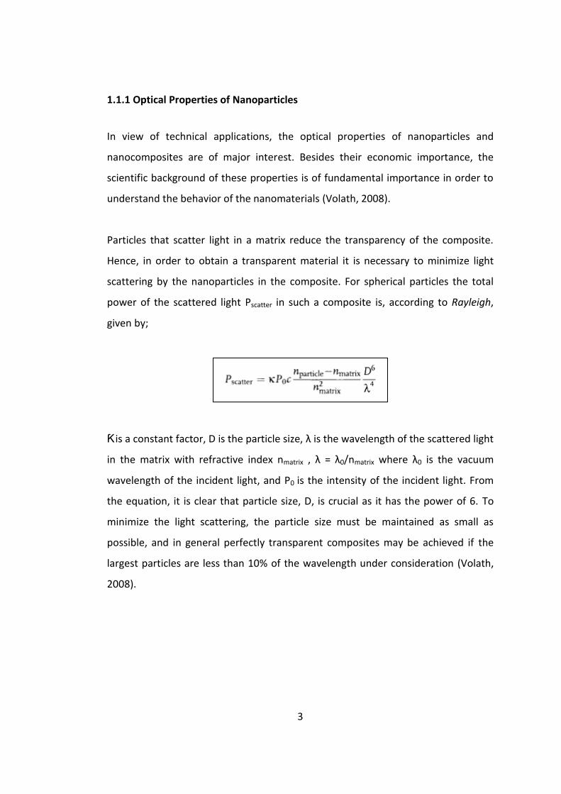
Particles that scatter light in a matrix reduce the transparency of the composite.

Hence, in order to obtain a transparent material it is necessary to minimize light

scattering by the nanoparticles in the composite. For spherical particles the total

power of the scattered light Pscatter in such a composite is, according to Rayleigh,

given by;

Ƙ is a constant factor, D is the particle size, λ is the wavelength of the scattered light

in the matrix with refractive index nmatrix , λ = λ0/nmatrix where λ0 is the vacuum

wavelength of the incident light, and P0 is the intensity of the incident light. From

the equation, it is clear that particle size, D, is crucial as it has the power of 6. To

minimize the light scattering, the particle size must be maintained as small as

possible, and in general perfectly transparent composites may be achieved if the

largest particles are less than 10% of the wavelength under consideration (Volath,

2008).

4

1.1.2 Magnetic Properties of Nanoparticles

Magnetism derives from the spin and orbital behavior of electrons. Nanoparticles

are behaving differently with respect to their behavior in magnetic field (Kumar,

2009). In general, materials are divided in diamagnetic, paramagnetic or

ferromagnetic with respect to their response to an external magnetic field (Volath,

2008) and types of magnetism are explained as follows.

1.1.2.1 Diamagnetism

Materials with filled electron shells in which all electrons are paired are said to be

diamagnetic. Different orientations of diamagnetic materials are shown in Figure 2

(Greg Goebel). thus, the magnetic dipoles of their individual electrons cancel out

and they exhibit low negative susceptibility (weak repulsion) in magnetic field.

Examples of diamagnetic materials are copper, gold and silver (Kumar, 2009).

Figure 2. Different orientations of diamagnetic materials

5

1.1.2.2 Paramagnetism

Materials with unpaired electrons in which the magnetic dipoles are oriented in

random directions at normal temperatures are said to be paramagnetic. Some of

these single-electron dipoles line up with an applied magnetic field and therefore

paramagnetic materials display low positive susceptibility (weak attraction) in

magnetic field; however, they do not remain magnetic when the field is removed,

because the ambient thermal energy is sufficient to reorientate the dipoles in

random directions (Kumar, 2009). Different orientations of paramagnetic materials

are shown in Figure 3 (Greg Goebel).

Figure 3. Different orientations of paramagnetic materials

Both, ferromagnetic and ferrimagnetic materials also contain unpaired electrons

although, unlike the unpaired electrons in paramagnetic materials, these are

organized into domains comprising the electrons of many atoms or ions. Each

domain is a single magnetic dipole that typically has dimensions of less than 100

6

nm. In an equilibrated ferromagnetic or ferrimagnetic material the magnetic dipoles

are organized in random directions; however, when a magnetic fields is applied

they are aligned even when the magnetic field is removed because the ambient

thermal energy is insufficient to reorientate them. Different orientations of

ferromagnetic materials are shown in Figure 4 (Greg Goebel). All ‘’permanent’’

magnets are made from ferromagnetic or ferrimagnetic materials; examples include

iron, cobalt, nickel, and magnetite (iron oxide) (Kumar, 2009).

Figure 4 Different orientations of ferromagnetic materials

1.1.2.3 Antiferromagnetism

Materials in which single electron magnetic dipoles are aligned in a regular pattern,

and in which the neighboring dipoles cancel out, are classified as

antiferromagnetics. When a ferromagnetic film is grown on or annealed to an

antiferromagnetic material in an aligning magnetic field, the direction of

magnetization in the ferromagnetic layer remains pinned in this direction when the

7

magnetic field has been removed. Typical examples of antiferromagnetic materials

are chromium and nickel oxide (Kumar, 2009).

1.1.2.4 Superparamagnetism

Because both ferromagnetic and ferrimagnetic materials depend on their domain

structure in order to remain magnetic in the absence of an applied field, their

properties undergo an important change when their dimensions are decreased to

less than domain size. Particles of this size are said to be superparamagnetic

because, although their dipoles line up parallel to an applied magnetic field, the

ambient thermal energy is sufficient to spontaneously disorganize the direction of

their magnetization when the field is no longer applied. This is important for

biothechnology applications, because it would not be possible to resuspend

magnetic particles in solution following a magnetic separation due to mutual

attraction if they remained magnetic. The force (magnetic moment) experienced by

a particle depends on the strength of the applied field and the size and composition

of the particle (Kumar, 2009).

1.1.2.5 Magnetization Hysteresis Loop

The magnetization hysteresis loop shows the behavior of a sample when an

external magnetic field is applied. It can be obtained by minimizing the total free

energy of the sample in this field (Sun, Y., Chien, & Searson, 2005).

There are many factors that alter the hysteresis loop of a sample. These are the

type, shape, structure and size of the material and the orientation of the

magnetizing field. The interactions between the particles may also change the

8

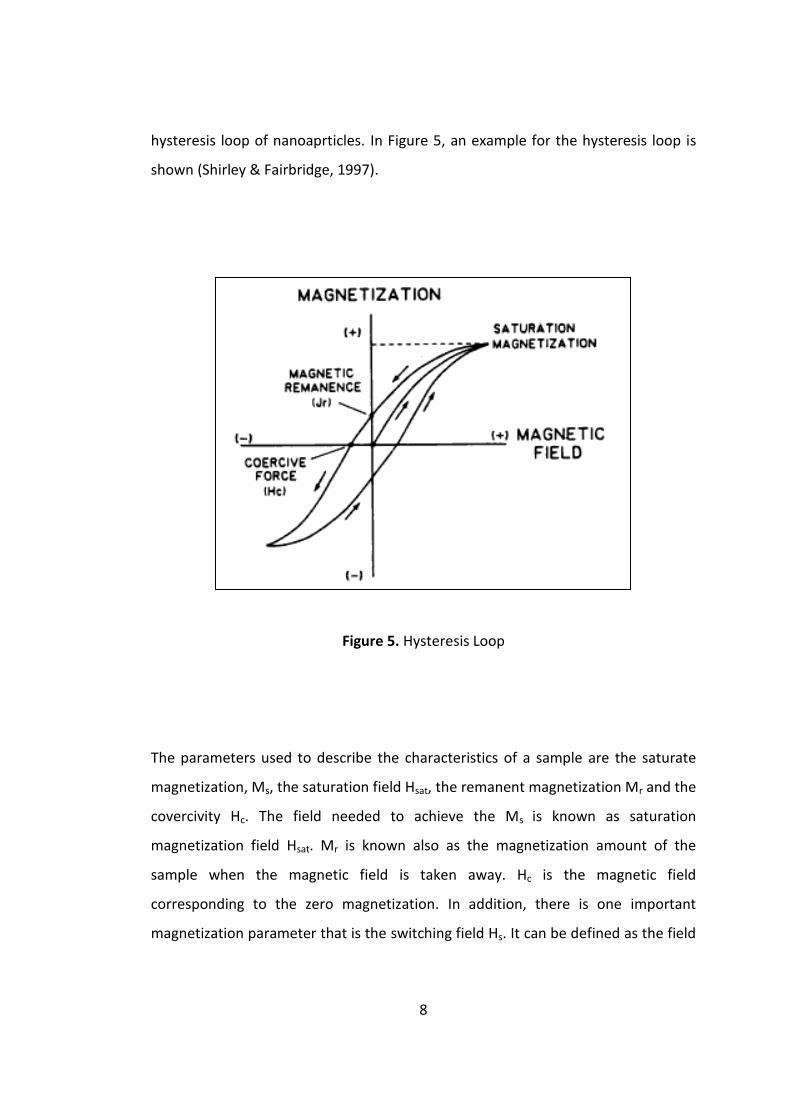
hysteresis loop of nanoaprticles. In Figure 5, an example for the hysteresis loop is

shown (Shirley & Fairbridge, 1997).

Figure 5. Hysteresis Loop

The parameters used to describe the characteristics of a sample are the saturate

magnetization, Ms, the saturation field Hsat, the remanent magnetization Mr and the

covercivity Hc. The field needed to achieve the Ms is known as saturation

magnetization field Hsat. Mr is known also as the magnetization amount of the

sample when the magnetic field is taken away. Hc is the magnetic field

corresponding to the zero magnetization. In addition, there is one important

magnetization parameter that is the switching field Hs. It can be defined as the field

9

at which M-H loop slope reaches the maximum value. Hs is used to analyze

magnetic nanomaterials (Varadan, 2008; Dionnei, 2009).

1.1.3 Iron Oxide Nanoparticles

Iron oxides are widespread in nature. They are in soils and rocks, lakes and rivers,

on the sea floor etc. Because of their properties and processes they are very

important and have attracted great attention. In living organisms, iron oxides may

be present as an iron reservoir such as ferritin, as hardening agents in teeth

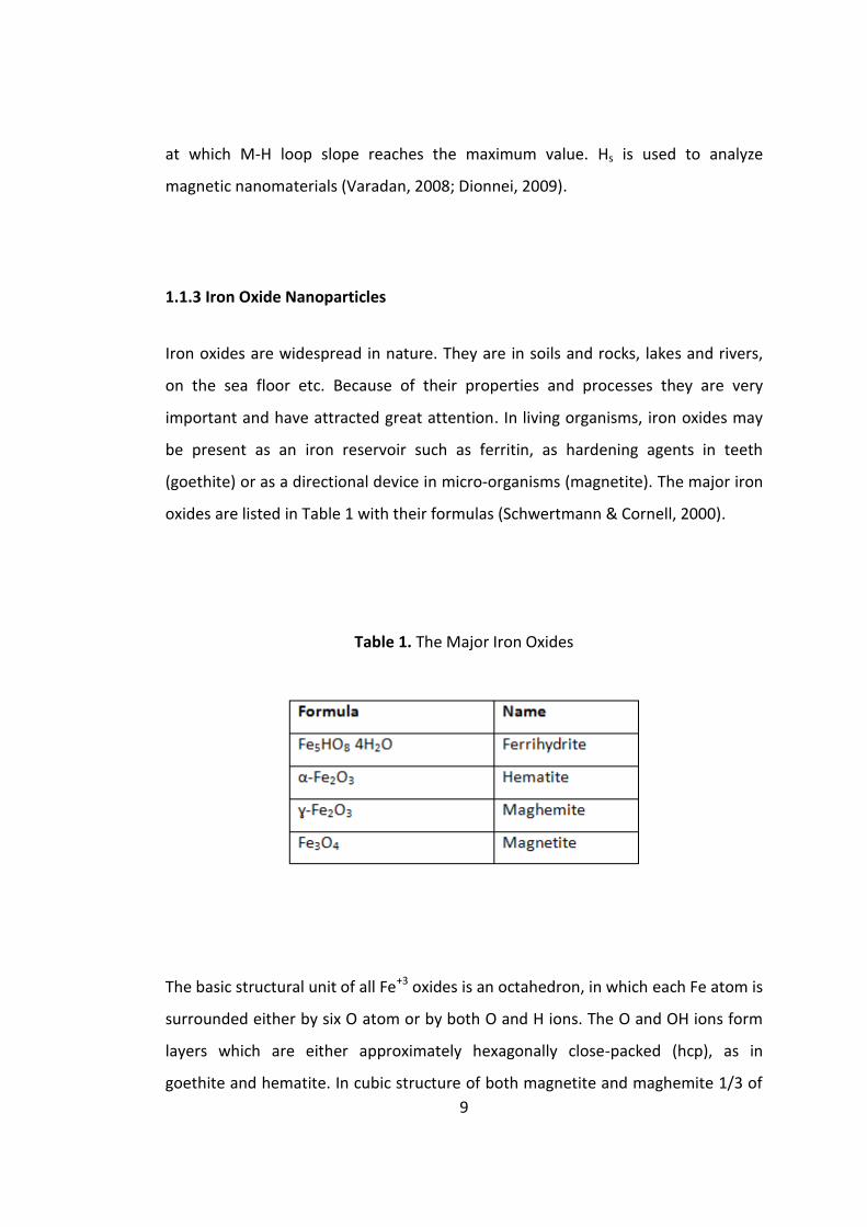
(goethite) or as a directional device in micro-organisms (magnetite). The major iron

oxides are listed in Table 1 with their formulas (Schwertmann & Cornell, 2000).

Table 1. The Major Iron Oxides

The basic structural unit of all Fe+3 oxides is an octahedron, in which each Fe atom is

surrounded either by six O atom or by both O and H ions. The O and OH ions form

layers which are either approximately hexagonally close-packed (hcp), as in

goethite and hematite. In cubic structure of both magnetite and maghemite 1/3 of

10

the interstices are tedrahedrally coordinated with oxygen and 2/3 are octahedrally

coordinated. In magnetite all of these positions are filled with Fe. In Figure 6 it was

shown that magnetite is an inverse spinel: the tedrahedral positions are completely

occupied by Fe+3, the octahedral ones by equal amounts of Fe+3 and Fe+2

(Schwertmann & Cornell, 2000; Gossuin, Gillis, A., Vuong, & Roch, 2009). The

electrons can hop between Fe+2 and Fe+3 ions in the octahedral sites at room

temperature, rendering magnetite an important class of half-metallic materials

(Kwei, von Dreele, Williams, Goldstone, Lawson, & Warburton, 1990). Maghemite

has a structure similar to that of magnetite. It differs from magnetite in that all or

most Fe is in Fe+3 state (Cornell & Schwertmann, 2003).

Figure 6. Inverse spinel structure of magnetite

11

Moreover, magnetite is ferromagnetic at room temperature and has a Curie

temperature (Tc) of 850 K. Maghemite is also ferromagnetic at room temperature.

It is difficult to measure Tc of maghemite since it transforms to hematite at high

temperatures (Cornell & Schwertmann, 2003). Hematite is an antiferromagnetic

material below the Morin transition at 250 K, and weakly ferromagnetic at room

temperature (above the Morin transition and below its Néel temperature at 948 K,

above which it is paramagnetic).

Regarding the choice of magnetic nanoparticle, magnetite and maghemite are the

most studied because of their generally appropriate magnetic properties and

biological compability (Pankhurst, Connolly, S., & J., 2003). These iron oxide

nanoparticles can be used in many applications such as magnetic resonance

imaging contrast enhancement, (Babes, Denizot, Tanguy, Jacques, Jeune, & Jallet,

1999) tissue repair, drug delivery (Gupta & Gupta, 2005) and radioactive imaging

(Hafeli, Pauer, Failing, & Tapolsky, 2001) due to these mentioned properties. All of

these biomedical applications require that the nanoparticles have high

magnetization values, a size smaller than 100 nm and a narrow particle size

distribution (Laurent, et al., 2008).

1.1.3.1 Synthesis of Magnetic Iron Oxide Nanoparticles

There are lots of procedures and methods in order to synthesize magnetic iron

oxide nanoparticles, magnetite and maghemite. These are summarized as follows.

Coprecipitation is one of the most commonly used methods. Iron oxide

nanoparticles are synthesized through the coprecipitation of Fe+3 and Fe+2 aqueous

salt solutions by addition of base (Gupta & Gupta, 2005; Ma, Zhang, Yu, Shen,

12

Zhang, & Gu, 2003; Liang, Wang, yu, Zhang, Xia, & Yin, 2007). This was followed by

collecting the precipitated iron oxides by magnetic separation.

Polyol method is also used by many researchers. Nanoparticle synthesis starts by

dissolving iron salts in organic solvent (such as ethylene glycol) in this method. Then

base is added to solution and solution is incubated at high temperatures (Zhao, et

al., 2007). The solvents have crucial role for this method. They are able to dissolve

inorganic compounds because of their high dielectric constants. It is suitable to

study in a wide range of temperatures owing to their high boiling points. Finally,

they also behave as reducing agents besides being stabilizer which provides control

of the particle size (Laurent, et al., 2008).

Iron oxide nanoparticles can also be synthesized by microemulsion method (Gupta

& Wells, 2004). This method is based on the encapsulation of nanoparticles in

micelles (Schmid, 2010).

Sonochemistry is applied to obtain nanoparticles. By applying ultrasound vibration

nanoparticles are synthesized. This method is more useful to obtain smaller

nanoparticles than the method in which ultrasound is not used for power of

ultrasound prevents nanoparticles from agglomeration (Morel, et al., 2008).

Thermal decomposition is a method especially preferred to synthesize smaller

nanoparticles among the other methods. Iron precursors are cracked at high

temperatures by using organic solvents and surfactants (Karlsson, Deppert,

Karlsson, & Malm, 2005). There are many factors affecting the size and morphology

of the nanoparticles during the synthesis by this method. These are the reaction

times and the temperature, nature of the solvent, precursors, concentration and

ratios of the reactants (Laurent, et al., 2008).

13

Aerosol pyrolysis method is also applied for synthesis of iron oxide nanoparticles. A

nebulizer is used in this method to inject very small droplets of precursor solution.

Reaction takes place in solution in the droplets. After the reaction is completed,

solvent is evaporated from the medium and solid nanoparticles are obtained

(Martinez, Roig, Molins, Gonzalez-Carreno, & Serna, 1998; Tartaj, Gonzalez-

Carreno, Rebolledo, Bomati-Miguel, & Serna, 2007; Swihart, 2003).

1.1.3.2 Surface Modification of Iron Oxide Nanoparticles

Surface modification is very crucial for nanoparticles in order to combine new

functional groups with nanoparticles. During the surface modification particles size

distribution especially for magnetic nanoparticles should be narrow enough to be

applied in many areas (Cao, Zhang, & Brinker, 2010).

Surface modification of iron oxide nanoparticles requires more attention because

they should be chemically stable and homogeneously dispersed in the medium to

be able to use them in biotechnology and biomedicine. Since iron oxide

nanoparticles are easily aggregate owing to the anisotropic dipolar attraction and

form large clusters which causes losing some properties of it, surface modification

of these nanoparticles is very essential. In addition, biocompability of the

nanoparticles is prevented by surface modification (Ma, Guan, & Liu, 2006).

1.1.3.2.1 Silica Coating

Silica coating has many advantages. First, it protects nanoparticles from

agglomeration (Ma, Guan, & Liu, 2006). Second, it prevents undesired reactions. For

example, the interaction of dye molecules with nanoparticles usually results in

14

luminescence quenching. To overcome this problem, nanoparticles first coated with

silica and then dye molecules were attached on the silica shell (Ma D. , et al., 2006).

Third, stable nanoparticles are obtained by silica coating. Final advantage of silica

coating is providing easy further surface modification (Hu, Salabas, & Schüth, 2007).

For silica coating the most frequently used method is known as sol-gel method. In

this method, silica phases are formed on colloidal magnetic nanoparticles in a basic

alcohol/water mixture (Lu, Yin, Mayers, & Xia, 2002). In literature, this method is

also named as Stöber method (Liz-Marzan M. L., 1996). The thickness of silica layer

can be adjusted by varying the concentration of base and the ratio of silica

precursor to H2O. Since silica coating was performed on an oxide surface, further

surface modification can easily be done by OH surface groups (Hu, Salabas, &

Schüth, 2007).

The second method for silica coating of nanoparticles is synthesizing nanoparticles

inside the pores of pre-synthesized silica (Deng, Wang, Hu, Yang, & Fu, 2005).

Aerosol pyrolysis is the third method. In this method, a mixture of silicon precursor

and metal precursor is sent to furnace in an aerosol form (Morales, Gonzalez-

Carreno, Ocana, Alonso-Sanudo, & Serna, 2000). Rapid synthesis of nanoparticles

can be achieved with this method.

1.1.3.2.2 Silanization

Silica shell does not only protect the magnetic nanoparticles against degradation,

but can also be used for further functionalization such as silanization (Lu, Salabas, &

Schüth, 2007). Several silanization processes are shown in Figure 7 (Boisseau,

Houdy, & Lahmani, 2007). During the silanization, two reactions take place

15

simultaneously. Hydrolysis of the n silane hydroxyl groups to the reactive silanol

species and the condensation of this silanols with the free OH groups of the surface

are taken place and stable Si-O-Si bonds are formed with covalent binding.

Temperature, solvent type and time are some variables that affect reaction (He,

2005; Bruce & Sen, 2005).

Figure 7. Reaction mechanism of several silanization processes

3-aminopropyltriethoxy silane (APTES) (Ma, Zhang, Yu, Shen, Zhang, & Gu, 2003), 3-

aminopropyltrimethoxy silane (APS) (Liz-Marzan M. L., 1996) and N-(2-aminoethyl)-

3 aminopropyltrimethoxy silane (AEAPS) (Liang, Wang, yu, Zhang, Xia, & Yin, 2007)

are the main amine precursors used in the literature for silanization purpose and

16

detailed silanization reaction mechanism of APTES with nanoparticle is shown in the

Figure 8 (Boisseau, Houdy, & Lahmani, 2007).

Figure 8. Surface modification of nanoparticles with APTES in aqueous medium: (a)

Hydrolysis in solution. (b) Self-condensation. (c) Attaching on surface of

nanoparticles.

1.1.3.2.3 Histidine Immobilization

Besides attaching amine groups on the surface of the nanoparticles, surface

modification with biological compounds is needed to get biocompatible systems.

This process also provides better selectivity and targeting capability for another

study (Cao, Zhang, & Brinker, 2010). Biological compounds are bounded to the

surfaces of the nanoparticles by chemically coupling with the help of amide or ester

bonds (Gupta & Gupta, 2005).

Histidine is preferred as a biological compound for surface modification of magnetic

nanoparticles and other purposes (Çorman, Öztürk, Bereli, Akgöl, Denizli, & A.,

2010; Lim, Lee, Lee, & Chung, 2006; Kröger, Liley, Schiweck, Skerra, & Vogel, 1999;

17

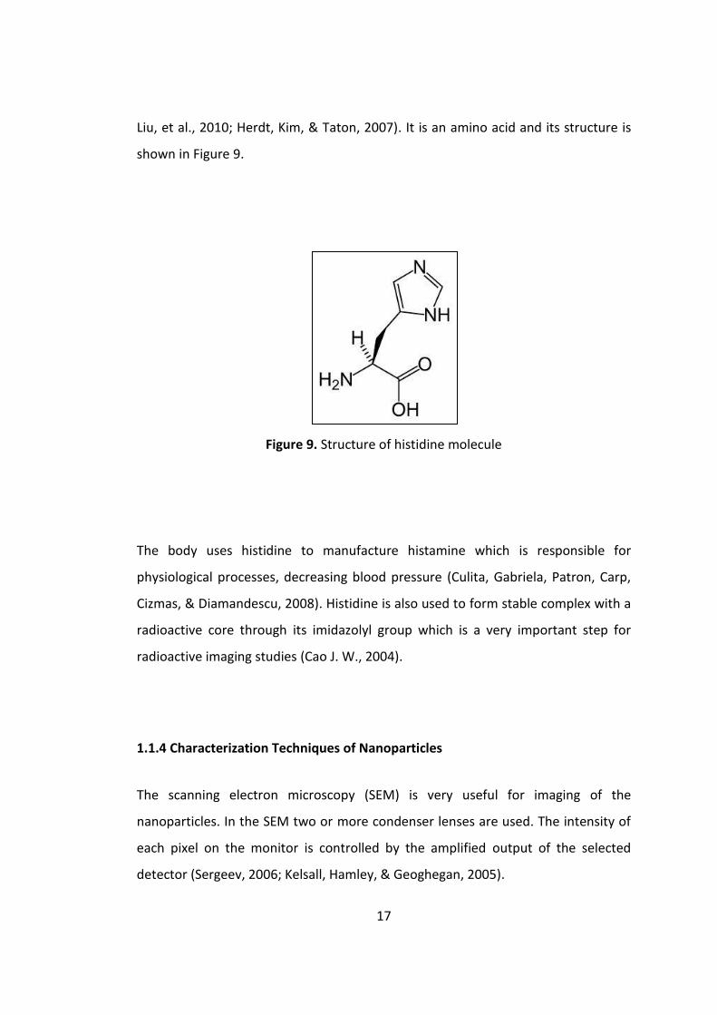
Liu, et al., 2010; Herdt, Kim, & Taton, 2007). It is an amino acid and its structure is

shown in Figure 9.

Figure 9. Structure of histidine molecule

The body uses histidine to manufacture histamine which is responsible for

physiological processes, decreasing blood pressure (Culita, Gabriela, Patron, Carp,

Cizmas, & Diamandescu, 2008). Histidine is also used to form stable complex with a

radioactive core through its imidazolyl group which is a very important step for

radioactive imaging studies (Cao J. W., 2004).

1.1.4 Characterization Techniques of Nanoparticles

The scanning electron microscopy (SEM) is very useful for imaging of the

nanoparticles. In the SEM two or more condenser lenses are used. The intensity of

each pixel on the monitor is controlled by the amplified output of the selected

detector (Sergeev, 2006; Kelsall, Hamley, & Geoghegan, 2005).

18

In transmission electron microscopy (TEM), sample is irradiated with an electron

beam of uniform current density. Emitted electrons are passed through the

electron gun and condenser lens system (three or four lenses). Then, the image of

the electron intensity is taken and recorded by a detector (Reimer & Kohl, 2008;

Lue, 2001).

Elemental analysis can be done by energy dispersive X-ray spectrometer ( EDX )

which is generally combined with SEM or TEM. When the electron beam strikes the

specimen surface, not only secondary electrons and backscattered electrons but

also characteristic X-rays are generated at or near the specimen surface. The

characteristic X-rays are used to identify the composition and measure the

abundance of the elements in the specimen (Thomas & Stephen, 2010).

X-ray diffractometry (XRD) is also used for characterization of nanoparticles. X ray

source, specimen and detector are the main components of it and all these

components lie on the circle known as focusing circle inside the instrument. The X

ray source is stable and the detector moves through a range of angles. The choice

of the range depends on the crystal structure of the material and the time for

obtaining diffraction pattern (Suryanarayana & Norton, 1998).

1.2. Radiation Chemistry

The radiation chemistry in general depends on the discovery of X-rays by Wilhelm

Conrad Röntgen in 1895 and of radiochemistry by Henri Becquerel in the following

year. After the discoveries some observations were made. Discharge tubes and salts

of uranium emitted rays which were able to pass through nontransparent materials

and activate photographic emulsions. Marie Curie discovered radium and polonium

elements in 1898 by comparing ionization amount created by several uranium

19

minerals and salts. This discovery and the isolation of radium in appreciable

amounts was important for radiation chemistry, because it provided a relatively

source of radiation (Spinks & Woods, 1976; Friedlander, 2008).

Radiation from radium on water was one of the first reactions to be studied. In

1901 Marie Curie and André Louis Debierne found continuous gas production from

hydrated salt of radium and the evolution of gas from aqueous solution of radium

bromide was observed by Friedrich Oskar Giesel in 1902 (Spinks & Woods, 1976).

1.2.1 Sources of Radiation

The radiation chemistry benefits from the two types of radiation sources, namely

natural or artificial radioactive sources and those that employ some form of particle

accelerator. Some radioactive isotopes which are used as a radiation sources with

their type, half-life and energy of the radiation are listed in Table 2.

20

Table 2. Some Radioactive Isotopes Commonly Used as Sources of Radiation

Isotope

Half-life

Type and Energy (in MeV) of Principal

Radation Emitted

Natural Isotopes

Polonium-210 138 days α, 5.304 ( 100 % )

Ȣ, 0.8 ( 0.0012 % )

Radium-226 1620 years α, 4.777 ( 94.3 % )

α, 4.589 ( 5.7 % )

Ȣ, 0.188 (~ 4 % )

( + radiation from decay products if

present )

Radon-222 3.83 days α, 5.49

( + radation from decay products if

present )

Artificial isotopes

Caesium-137 30 years ß, 1.18 (max) ( 8 % ) 0.24 ( av )

ß, 0.52 (max) ( 92 % )

Ȣ, 0.6616 ( 82 % )

Cobalt-60 5.27 years ß, 0.314 ( max ) 0.093 (av )

Ȣ, 1332

Ȣ, 1.173

Hydrogen-3

( tritium )

12.26 years ß, 0.018 ( max ) 0.0055 ( av )

Phosphorus-32 14.22 days ß, 1710 ( max ) 0.70 ( av )

Strontium-90 +

Yittrium-90

28.0 years

( Y90, 64 hours )

ß, 0.544 ( max ) 0.205 ( av )

ß, 2.25 ( max ) 0.93 ( av )

Sulfur-35 87.2 days ß, 0.167 ( max ) 0.049 ( av )

21

1.2.2 Radioactive Decay

The activity of all radioactive radiation sources falls, as the source grows older. The

activity (Ct) after a period of decay (t) is related to the original activity (Co) as shown

in the following equation.

Where Ct is the activity, t a period of decay, Co the original activity, λ the decay

constant (Spinks & Woods, 1976).

In a radioactive decay both mass number and atomic number are conversed due to

emitting α and/or ß rays (Choppin, Liljenzin, & Rydberg, 2002). α-particles are the

nuclei of helium atoms and the least penetrating of the radiations from radioactive

isotopes (Spinks & Woods, 1976). In some decays, nucleus emits an electron which

is also known as ß-particle (Turner, 2007). Another type of ray is also emitted during

the decay. It is the Ȣ-ray electromagnetic radiation of nucleus. α- and ß- particles

lose their energy step by step. Ȣ-rays, however, lose the greater part of their energy

by a single interaction (Spinks & Woods, 1976).

1.2.3 The Chemistry of Technetium

The element was first predicted by Mendeleev (eka-manganese, number 43) in

1872 and discovered by Segre and Perrier in 1938. It was named as ‘technetium’

which means artificial in Greek (Peacock, 1966; Dilworth & Parrott, 1998). Segre

and Perrier discovered the isotopes of technetium-95 and technetium-97. It was

22

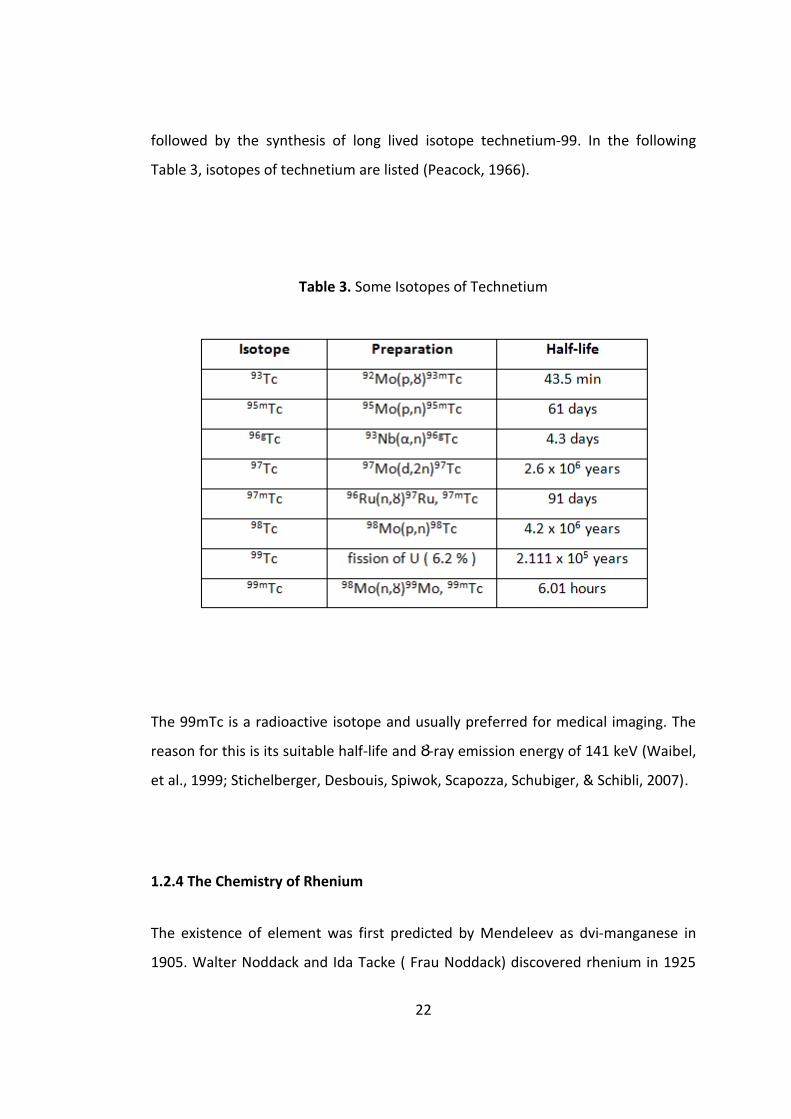
followed by the synthesis of long lived isotope technetium-99. In the following

Table 3, isotopes of technetium are listed (Peacock, 1966).

Table 3. Some Isotopes of Technetium

The 99mTc is a radioactive isotope and usually preferred for medical imaging. The

reason for this is its suitable half-life and Ȣ-ray emission energy of 141 keV (Waibel,

et al., 1999; Stichelberger, Desbouis, Spiwok, Scapozza, Schubiger, & Schibli, 2007).

1.2.4 The Chemistry of Rhenium

The existence of element was first predicted by Mendeleev as dvi-manganese in

1905. Walter Noddack and Ida Tacke ( Frau Noddack) discovered rhenium in 1925

23

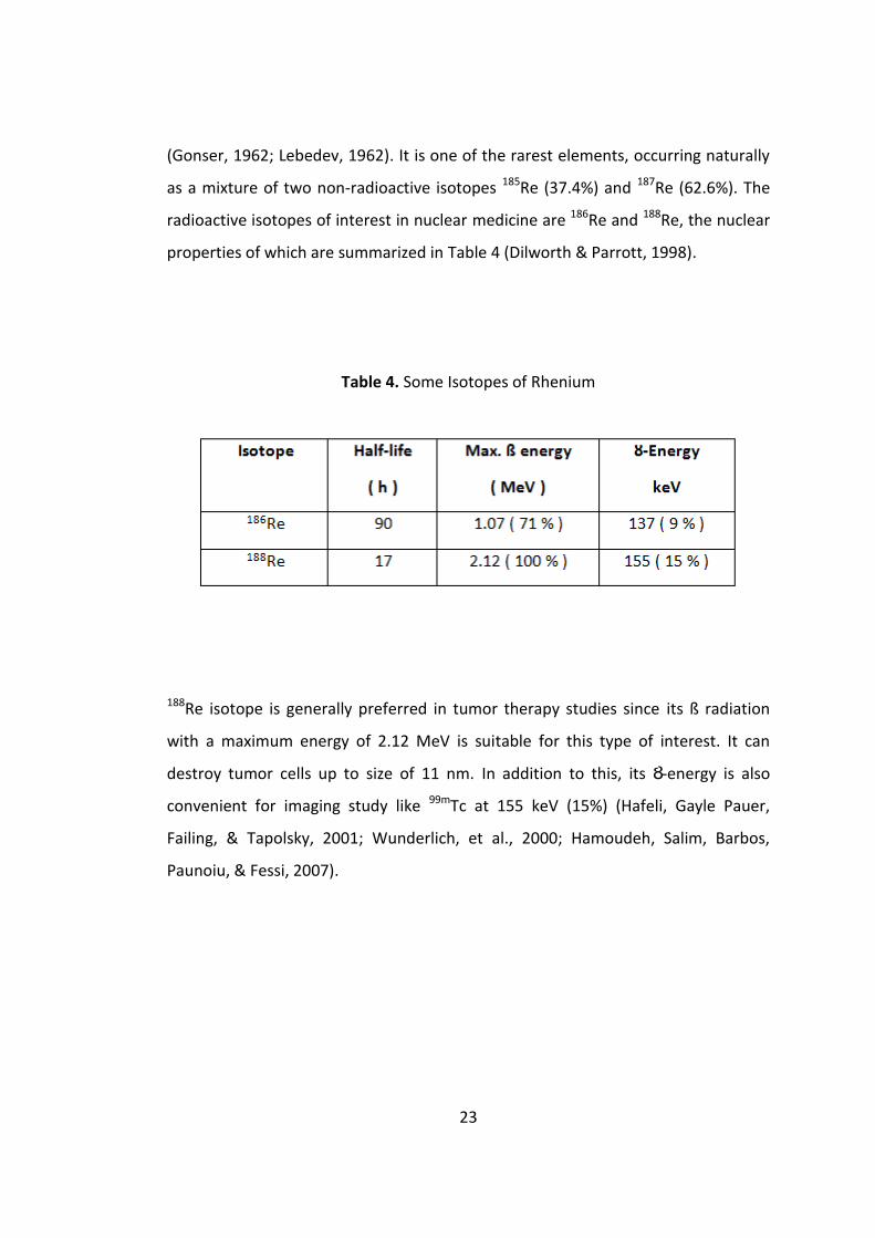
(Gonser, 1962; Lebedev, 1962). It is one of the rarest elements, occurring naturally

as a mixture of two non-radioactive isotopes 185Re (37.4%) and 187Re (62.6%). The

radioactive isotopes of interest in nuclear medicine are 186Re and 188Re, the nuclear

properties of which are summarized in Table 4 (Dilworth & Parrott, 1998).

Table 4. Some Isotopes of Rhenium

188Re isotope is generally preferred in tumor therapy studies since its ß radiation

with a maximum energy of 2.12 MeV is suitable for this type of interest. It can

destroy tumor cells up to size of 11 nm. In addition to this, its Ȣ-energy is also

convenient for imaging study like 99mTc at 155 keV (15%) (Hafeli, Gayle Pauer,

Failing, & Tapolsky, 2001; Wunderlich, et al., 2000; Hamoudeh, Salim, Barbos,

Paunoiu, & Fessi, 2007).

24

1.2.5 Radioactive Imaging

Radioactive imaging is principally based on the external detection of radionuclide

emitted by a reported located in the body (Ottobrini, Ciana, Biserni, Lucignani, &

Maggi, 2006; Thorek, Chien, Czupryna, & Tsourkas, 2006).

By injecting a patient with radioisotope, regions of high metabolic activity may be

imaged by the anomalous concentration of the isotope there. For this to be

effective most of the radiation from the decay should escape the body without

attenuation or being scaterred, and the half-life of the decay should be matched

with the duration of the procedure. Such a long decay time is only possible either

with a highly suppressed electromagnetic decay or with a prompt electromagnetic

process following weak interaction decay (Allison, 2006).

Radionuclide imaging is commonly devised into two general modalities; single

photon emission computed tomography (SPECT) and positron emission tomography

(PET) (Hamoudeh, Kamleh, Diab, & Fessi, 2008). PET is a noninvasive nuclear

imaging technique that produces images of the metabolic activity of living

organisms on the biomedical level. These images are detected by introducing a

short-lived positron emitting radioactive tracer, or radiopharmaceutical, by either

intravenous injection or inhalation. Images are created using a process called

radioactive labeling in which one atom in a molecule is replaced by radioactive one

(Jarrett, Gustafsson, Kukis, & Louie, 2008).

PET images help physicians identify normal and abnormal activity in living tissue.

PET recognizes the metabolic changes by measuring the amount of radioactive

tracers distributed through the body. This information is subsequently used to

create a three dimensional (3D) image of tissue function from the acquired decay

matrix (Najariani & Splinter, 2006).

25

The functional imaging features of PET are most prominent in the diagnosis of

cancer. Healthy tissue replenishes its cells by continuous regeneration, while old

cells gradually die off. In many cases the PET features can identify diseases earlier

and more specially than ultrasound, X-rays, computed tomography (CT) or magnetic

resonance imaging (MRI) (Kairemo, Erba, Bergström, & Pauwels, 2008; Lucignani,

Ottobrini, Martelli, Rescigno, & Clerici, 2006).

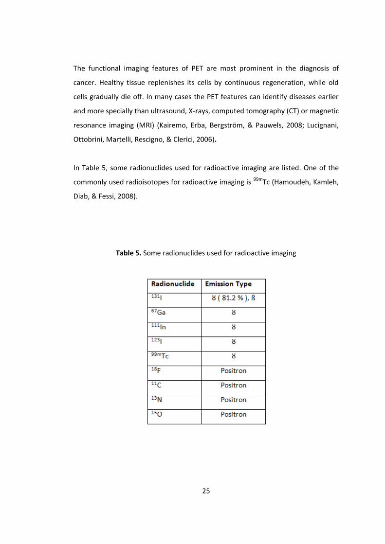
In Table 5, some radionuclides used for radioactive imaging are listed. One of the

commonly used radioisotopes for radioactive imaging is 99mTc (Hamoudeh, Kamleh,

Diab, & Fessi, 2008).

Table 5. Some radionuclides used for radioactive imaging

26

The technetium eluate is injected into a vial, which is including the necessary

reagents to produce the imaging agent. The radiopharmaceutical is injected into

the patient after a suitable incubation period. In Figure 10, a patient is shown who

is undergoing a radioactive imaging. Following the distribution of the

pharmaceuticals in the whole body, the image data are gathered by a Ȣ camera that

is equipped with a NaI scintillation detector and photomultiplier system (Dilworth &

Parrott, 1998).

Figure 10. A patient undergoing a radioactive imaging by a gamma camera.

27

The camera is rotated around the patient or a multidetector array is used to create

an image with the help of software program. During this process, the total radiation

dose is comparable with that from a conventional X-ray (Dilworth & Parrott, 1998).

1.3 Aim of the Study

The purpose of this study is the preparation of surface modified magnetite

nanoparticles and rhenium carbonyl complex. Finally, the surface modified

magnetite nanoparticles will be labeled with the rhenium- carbonyl complex. All

necessary optimization and characterization studies will be carried out.

28

CHAPTER 2

EXPERIMENTAL

2.1 Chemical and Reagents

Oxygen (O2) free water was used during the synthesis and silica coating of

magnetite nanoparticles. It was obtained by sending nitrogen gas for 45 min from

deionized water obtained from a Millipore system (Molsheim, France). Technical

ethanol ( EtOH ) was preferred when washing process was applied.

All chemicals and reagents were expressed in the order of their name, chemical

formula, purity and manufacturer name.

2.1.1 Synthesis of Magnetite Nanoparticles

i. Iron(III) chloride reagent grade, FeCl3, ˃97 %, Sigma-Aldrich

ii. Iron(II) sulfate heptahydrate puriss, FeSO4∙7H2O, 99.5-104.5 %, Riedel-de Haën

iii. Hydrochloric acid (HCl), 37%, Merck

iv. Ammonia solution, 25% extra pure, Merck

v. EtOH, (CH3CH2OH), 99.5%, Sigma-Aldrich

vi. Nitrogen gas (N2), pure, Habaş Sınai ve Tıbbi Gazlar İstihsal Endüstrisi A.Ş

29

2.1.2 Silica Coating on Magnetite Nanoparticles

i. (3-Aminopropyl)triethoxysilane, APTES, C9H23NO3Si, ≥ 98.0%, Fluka

ii. Tetraethy ortosilicate, TEOS, Si(OC2H5)4 98%, Aldrich

iii. EtOH, (CH3CH2OH), 99.5%, Sigma-Aldrich

2.1.3 Surface Modification of Magnetite Nanoparticles with APTES

i. (3-Aminopropyl)triethoxysilane, APTES, C9H23NO3Si, ≥ 98.0, Fluka

ii. EtOH, (CH3CH2OH), 99.5%, Sigma-Aldrich

iii. Deionized water

2.1.4 Immobilization of Histidine

i. MeOH G for gradient elution, CH4O, Sigma-Aldrich

ii. 0.1 M phosphate buffer solution, PBS, (K2HPO4, KH2PO4 and H2O), pH 7.4

iii. 2.5 % Glutaraldehyde, OHC(CH2)3CHO, Grade I, 25 % Sigma Aldrich

iv. L-Histidine, C6H9N3O2, ≥ 99 %, Sigma-Aldrich

v. Sodium chloride, NaCl, ≥ 99 %, Merck

vi. Ethylenediaminetetraaceticacid (EDTA) disodium salt dihydrate, C10H16N2O8, %,

Carlo Erba Reagenti

vii. 0.1 M Sodium borate buffer solution, (Sodium hydroxide, borax and water), pH

9.2

viii. Sodium borohydride GR for analysis, NaBH4, ≥ 96 %, Merck

ix. MES buffer solution

30

2.1.5 Rhenium Complex Formation

‘Rhenium complex’ or ‘rhenium carbonyl complex’ will be used instead of

[Re(CO)3(H2O)3]+from now on.

i. Borane-ammonia complex, BH3NH3, 97%, Aldrich

ii. Carbon monoxide gas, CO(g), pure, OKSAN Tıbbi Gazlar Üretim Sanayi ve Ticaret

Anonim Şirketi

iii. Sodium perrhenate, NaReO4, 99.99% metal basis, Aldrich

iv. Phosphoric acid, H3PO4, 85%, J. T. Baker

2.2 Procedure

2.2.1 Synthesis of Magnetic Iron Oxide Nanoparticles, Magnetite

First part of this study was the synthesis of magnetic iron oxide nanoparticles.

Mainly the method of Molday (Molday, 1984) was followed. The reaction regarding

magnetite synthesis was given in the following equation (Cao J. W., 2004) and the

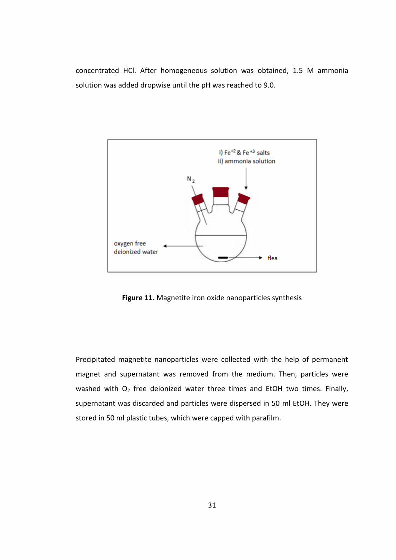
experimental set up was shown in Figure 11.

6Fe3+ + SO32- + 18NH4OH → 2Fe3O4 + SO4

2- + 18NH4+ + 9H2O

Procedure of magnetite synthesis can be explained as follows. 0.29196 g FeCl3 salt

and 0.25021 g FeSO4∙7H2O salt were weighed into a three necked round bottom

flask and 150 ml of O2 free deionized water were added. Precursor solution was

stirred on magnetic plate with a stir bar immersed in the solution. The system was

kept under N2 atmosphere. pH of the solution was adjusted to 1.7 with

31

concentrated HCl. After homogeneous solution was obtained, 1.5 M ammonia

solution was added dropwise until the pH was reached to 9.0.

Figure 11. Magnetite iron oxide nanoparticles synthesis

Precipitated magnetite nanoparticles were collected with the help of permanent

magnet and supernatant was removed from the medium. Then, particles were

washed with O2 free deionized water three times and EtOH two times. Finally,

supernatant was discarded and particles were dispersed in 50 ml EtOH. They were

stored in 50 ml plastic tubes, which were capped with parafilm.

32

2.2.2 Silica Coating on Magnetite Nanoparticles

Silica coating was the next step after synthesizing iron oxide nanoparticles. APTES

and TEOS were used for this purpose (Liz-Marzan M. L., 1996). The reaction of silica

coating was indicated in Figure 12.

Figure 12. Silica coated magnetite

Magnetite particles dispersed in ethanol (magnetite solution) was placed into

ultrasonic bath for 15 minutes. 13.89 ml of the magnetite solution were taken.

Particles were collected with the help of magnet since they were dispersed in EtOH.

Supernatant was discarded and precipitated particles were dispersed in 500 ml O2

free deionized water. Then, freshly prepared 2.5 ml 1 mM APTES solution were

added into solution. It was stirred strongly for 15 minute. Particles were collected

by magnet and supernatant solution was removed from the medium. Particles were

dispersed in 500 ml of deionized water/EtOH solution in 1:4 (v/v) ratio. Then, 300 µl

of TEOS and 2 ml of 28% ammonia solution were added. Solution was mixed for 12

h under mild stirring. Supernatant was removed and particles were washed with

33

deionized water and EtOH two times, separately. Finally, particles were dispersed in

50ml of EtOH. They were stored in a 50 ml plastic tube capped with parafilm.

2.2.3 Surface Modification of Magnetite Nanoparticles with APTES

After silica coating, surface of the nanoparticles was modified by using APTES (Ma

M. Z., 2003). The reaction of amine modification was shown in the Figure 13. 25.6

ml of silica coated magnetite solution dispersed in EtOH were taken into a round

bottom flask. The solution was diluted to 60 ml by EtOH and 400 µl of deionized

water. Then, the flask was placed into ultrasonic bath for 30 minutes. 300 µl of

APTES were added into solution and the contents were stirred for 12 h. After

incubation, modified nanoparticles were collected by magnet and supernatant was

discarded. Then, particles were washed with EtOH five times and dispersed in 10 ml

EtOH.

Figure 13. Surface modification of magnetite nanoparticles by using APTES

34

2.2.4 Immobilization of Histidine

Histidine was used to create a suitable platform to combine surface modified

nanoparticles with rhenium complex (Cao J. W., 2004). 5.0 ml of nanoparticles

surface of which was modified with amine groups were taken into a small glass vial.

These particles were collected by magnet and supernatant was removed from the

medium. Then, particles were washed with 0.1 M PBS buffer (pH 7.4). This was

followed by the collecting particles by magnet and removing the supernatant.

Washed nanoparticles were dispersed in 1.0 ml 2.5 % glutaraldehyde in 0.1 M PBS

(pH 7.4) and put into ultrasonic bath for 15 min. They were incubated at 4 °C for 4

h. After incubation, particles were again collected by magnet and washed with 0.1

M PBS (pH 7.4) for five times. Then, they were dispersed in 1.0 ml of 0.2 M freshly

prepared L-Histidine solution in 0.1 M PBS, 0.15 M NaCl, 0.005 M EDTA (pH 7.2).

Particles were washed with 0.1 M borate buffer solution (pH 9.2) for five times after

12 h incubation at room temperature. Then, particles were dispersed in 0.1 M

borate buffer solution, which is containing 0.5 mg/ml NaBH4. Solution was kept at 4

°C for 30 min. Particles were washed with 0.1 M PBS for three times and finally

dispersed in 1.0 ml 0.5 M MES buffer solution (pH 6.6). They were stored in a glass

vial capped with rubber stopper. The reaction of tagging histidine on surface of the

nanoparticle was shown in Figure 14.

35

Figure 14. Preparation of histidine tagged magnetite nanoparticles.

36

2.2.5 Formation of Rhenium Complex

The complex form of rhenium was prepared with respect to the method of Schibli

(Schibli, 2002). Experimental set up of complex formation study was shown in

Figure 15. First, BH3NH3 was taken into a mortar and grinded well. Then, it was

sieved and placed into a 10 ml glass vial. A plastic stopper was used to cap the vial.

CO (g) was flushed into the vial at 1.0 atm pressure for 10 minutes. Afterward, 2.0 ml

4.4 x 10-5 M NaReO4 solution and 60 µl 85 % H3PO4 were mixed and then injected

into the vial. Solution was incubated at 80-90 °C for 15 minutes. A syringe was used

in order to keep the hydrogen gas balance. Final step was the waiting until the

temperature of the solution reaches to the room temperature before doing

analysis.

37

Figure 15. Experimental set up of rhenium complex formation study

2.2.6 Labeling of Histidine-immobilized Nanoparticles with Rhenium Complex

After rhenium complex was formed with the sufficiently high yield, nanoparticles

were labeled with rhenium complex. 500 µl of the complex solution and 500 µl of

histidine immobilized nanoparticle solution were mixed well. The final solution was

placed into a shaker thermostated at 70 °C for 40 minutes (Cao J. W., 2004).

Labeled magnetic nanoparticles were extracted from the solution by using magnet.

38

2.3 Instrumentation

Characterization studies were done to gather information about the size, shape and

form of the magnetite and silica coated magnetite nanoparticles, the spectroscopic

and chromatographic behavior of the surface modified nanoparticles.

During the batch studies, Nd2Fe14B magnet, heater shaker and ultrasonic bath (Elma

S40 H, Germany) were used for decantation and preventing agglomeration,

respectively.

2.3.1 Transmission Electron Microscope ( TEM )

Morphology and size of the nanoparticles were characterized by TEM (JEOL 2100F)

at METU Central Laboratory. EMS formvar carbon film on 200 mesh copper grid

was used for the measurements. After drying the sample on grid at room

temperature TEM measurements were performed.

2.3.2 Field Emission Scanning Electron Microscope ( FE-SEM )

Particle size and shape was also determined by QUANTA 400F FE-SEM in METU

Central Laboratory. Before the measurements, nanoparticles were dispersed in a

solvent and the solution was dropped on carbon tape sticked onto copper grids for

SEM measurements. After drying the nanoparticles at room temperature, they

were coated with Au-Pd.

39

2.3.3. Energy Dispersive X-ray Spectrometer ( EDX )

Elemental analysis of the magnetite and silica coated magnetite nanoparticles were

performed by energy dispersed X-ray spectrometer, which was equipped with FE-

SEM. The samples used for the elemental analysis were the same as used for FE-

SEM analysis.

2.3.4 X-Ray Diffractometer ( XRD )

The type of the iron oxide nanoparticles was determined by Rigaku Miniflex X-ray

diffractometer with Cu source operating at 35 kW and 15 mA. The analysis was

done between the angles of 5° and 75° with the speed of a ϴ / minute. ICDD X-ray

identification cards were used to compare the obtained result with the theoretical

ones.

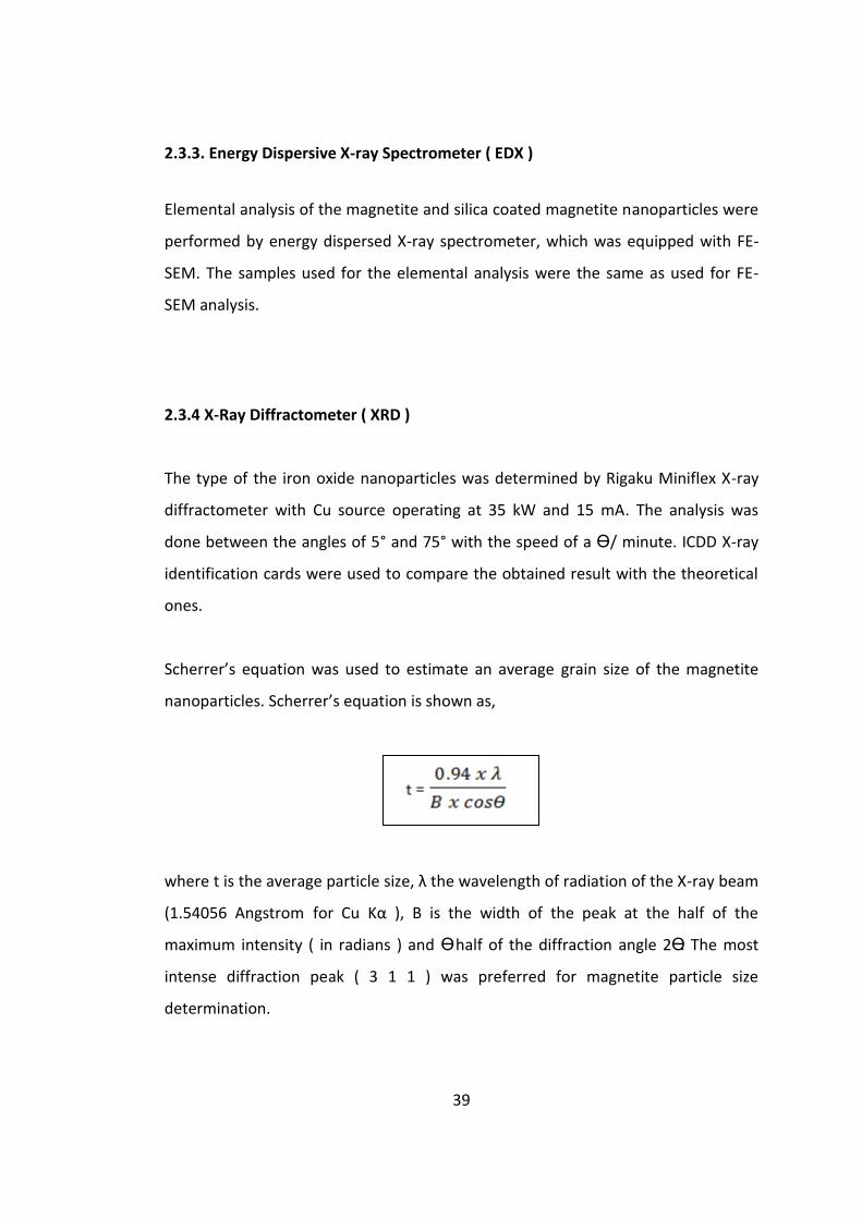
Scherrer’s equation was used to estimate an average grain size of the magnetite

nanoparticles. Scherrer’s equation is shown as,

where t is the average particle size, λ the wavelength of radiation of the X-ray beam

(1.54056 Angstrom for Cu Kα ), B is the width of the peak at the half of the

maximum intensity ( in radians ) and ϴ half of the diffraction angle 2ϴ. The most

intense diffraction peak ( 3 1 1 ) was preferred for magnetite particle size

determination.

40

In order to calculate the lattice constant of the samples, the Bragg’s Law was used,

where n is an integer determined by the order given, λ is the wavelength of X-rays,

d is the interplanar spacing between the planes in the atomic lattice, and θ is the

angle between the incident ray and the scattering planes. Then, using the following

equation for a cubic structure, the lattice constant, a, for the crystal structure was

calculated.

2.3.5 Vibrating Sample Magnetometer ( VSM )

Saturation magnetization value of the uncoated nanoparticles was measured by

VSM (Cryogenic Limited, Cryogen Free Vibrating Sample Magnetometer) at ± 1

Tesla at room temperature.

2.3.6 Surface Enhanced Raman Spectrometer ( SERS )

Magnetite nanoparticles were also characterized by Raman spectrometer (Jobin

Yvon LabRam confocal microscopy) equipped with a He-Ne (632.—nm) laser and a

charge coupled device (CCD) detector.

41

2.3.7 Zeta Potential Measurements

Malvern Nano ZS90 Systemin METU Central Laboratory was used for the zeta

potential measurements of the magnetite nanoparticles .

2.3.8 Particle Size Analyzer

Malvern Mastersizer 2000 in METU Central Laboratory was used for the particle size

distribution measurements for both magnetite and silica coated magnetite

nanoparticles.

2.3.9 Fourier Transform Infrared Spectrometer ( FT-IR )

Mainly for the characterization of the amine functionalized nanoparticles but also

for the magnetite and silica coated magnetite nanoparticles FT-IR (Alpha, Bruker)

was used in the range of 300 and 4500 cm-1. KBr pellets were prepared before the

analysis and stored in the desiccators in order to keep them away from moisture.

2.3.10 Inductively Coupled Plasma Optical Emission Spectrometer ( ICP-OES )

Copper and rhenium determinations were performed by ICP-OES (Direct Reading

Echelle, Leeman Labs INC.) for assessing the amine capacity of the silanized

nanoparticles. Some of the parameters used in ICP-OES measurements were as

follows: Incident plasma power was 1.2 kW, plasma coolant and the auxiliary Ar gas

flow rates were set at 18 L/min and 0.5 L/min respectively. The nebulizer Ar was

used at a pressure of 50 psi. Peristaltic pump at 1.2 ml/min flow rate was used for

42

sample transportation. Concentrations were determined at wavelength of 221.426

nm for Re and 324.754 nm for Cu.

2.3.11 High Performance Liquid Chromatogram Inductively Coupled Plasma Mass

Spectrometry ( HPLC-ICP-MS )

Formation of the rhenium carbonyl complex was examined by HPLC-ICP-MS

(Dionex, LPG-3400A model HPLC equipped with Thermo Electron Corporation X

Series model ICP-MS system) measurements in METU Chemistry Department

Analytical Chemistry Laboratory. S5 SAX anion exchange column and S5 SCX cation

exchange column were used as stationary phases. 5 mM sodium citrate in 10.0%

MeOH and 10 mM pyridine chloride in 5.0% MeOH were used as mobile phases.

Flow rate was adjusted to 1.50 ml/min for all analysis.

43

CHAPTER 3

REESULTS AND DISCUSSION

In this study, firstly magnetic iron oxide nanoparticles, namely magnetite, were

synthesized. Then, they were coated with silica and this was followed by surface

modification of these nanoparticles by amine. Next, histidine was attached to the

nanoparticles via glutaraldehyde spacer. Moreover, positively charged

Re(CO)3(H2O)3]+ complex was synthesized. Finally, nanoparticles were labeled with

Re(CO)3(H2O)3]+ complex.

3.1. Synthesis of Iron Oxide Nanoparticles, Magnetite

Co-precipitation method was used to synthesize magnetite nanoparticles, which

has a formulation of Fe3O4.

There are some points that need to be considered. One of them was easy oxidation

of magnetite nanoparticles. To prevent oxidation problem N2 (g) was used in many

times. First, it was used for obtaining oxygen free deionized water as a solvent.

Then it was purged through the reaction medium during the synthesis. Besides the

magnetite nanoparticle synthesized were stored in a plastic tube that was purged

with nitrogen before closed tightly.

Another criterion was dissolving iron precursors in water. A few drops of

concentrated HCl were used to dissolve precursors well in water. Then solution was

44

stirred strongly by using magnetic stirrer. Because of this process clear and

homogeneous iron salt solution was obtained.

Addition of ammonia solution into the iron precursor solution also played a crucial

role in the synthesis. The rate of ammonia addition was affecting the size of the

nanoparticles. Therefore, ammonia was added into the precursor solution dropwise

while the solution was stirred vigorously.

The magnetite particles were dried onto double-sided carbon tape and observed by

field emission scanning electron microscopy. The image of the magnetite

nanoparticles taken by FE-SEM in METU Central Laboratory is shown in Figure 16.

Visualization of structural details of specimens in FE-SEM requires optimal

conductivity. In general, Au/Pd, Pt or Cr with a thickness of 1.5-3.0 nm was

deposited on the specimen. In our measurements magnetite nanoparticles were

coated with Au-Pd to acquire a good contrast in imaging.

45

Figure 16. FE-SEM image of magnetite nanoparticles

From the FE-SEM image average particle size was calculated as 14 nm by selecting

10 particles from the image randomly and calculating the average of them.

The elemental analysis was performed by EDX and results of this characterization

study are shown in Figure 17.

46

Figure 17. EDX results of magnetite nanoparticles

As expected only Fe and O peaks appeared on the spectrum together with a high

carbon peak, which was coming from the carbon tape used for sampling.

Nanoparticles were also chacterized by FT-IR in order to show the chemical bonds

of Fe3O4. The FT-IR spectrum for these particles is shown in Figure 18.

47

Figure 18. FT-IR spectrum of the magnetite nanoparticles

In Figure 18, the peaks at 610 cm-1 and 440 cm-1 were assigned to Fe-O bond of

Fe3O4. Although, the characteristic absorption bands of the Fe-O bond of bulk Fe3O4

were stated as 570 and 375 cm-1, a blue-shift of absorption bands of the Fe-O to

around 600 and 440 cm-1, respectively, was reported for the Fe3O4 nanoparticles

(Ma M. Z., 2003). It was stated that as the particle size was reduced to nanosize,

large number of bonds for surface atom are broken, resulting in the rearrangement

of unlocalized electrons on the particle surface. As a result, lattice constrictions take

place and the surface bond force constant increases as Fe3O4 is reduced to

nanoscale dimension.

48

As EDX results, the IR spectrum also demonstrated the formation of the iron oxide

nanoparticles. The peaks at the 3427 and 1637 cm-1 were coming from the OH

vibrations of the water remaining in the sample. (Ma M. Z., 2003).

Since maghemite (-Fe2O3) and magnetite (Fe3O4) have similar peaks and behaviors,

further characterizations were done in order to differentiate the type of iron oxide

nanoparticles. For this purpose XRD analysis of one day, one month and one year

stored samples were carried out and the lattice constant values ( a ) were

calculated to predict the type of the nanoparticles.

XRD pattern of the nanoparticles stored for one day was shown in Figure 19.

Figure 19. X-Ray diffraction pattern of one day stored magnetite nanoparticles.

49

The data from Figure 19 were used for the calculation of the interplanar spacing (d)

between the planes in the atomic lattice, and the lattice constant (a), for the crystal

structure as described in section 2.3.4. The theoretical and calculated crystal

parameters of the one day stored magnetite nanoparticles were listed in Table 6.

Table 6. Theoretical ( ICDD Card No: 75-1610 ) and measured crystal parameters of

one day stored magnetite nanoparticles

The lattice constant value ( a ) is useful to determine the type of the nanoparticles.

This value is 0.833 nm for maghemite and 0.839 nm for magnetite (Mineralogy

Database). It can be seen from Table 6 that one day stored sample has lattice

constant values in between 0.833 and 0.837 nm. Thus it was not in pure magnetite

form but a mixture of magnetite and maghemite. High tendency of magnetite

towards oxidation was the reason for the occurrence of maghemite.

An average particle size of the one day stored samples was calculated by using

Scherrer’s equation. The most intense peak which was 3 1 1 used for this purpose

and average primary particle size was found as approximately 6.0 nm.

50

XRD pattern of the one month stored nanoparticles is shown in Figure 20.

Figure 20. X-Ray diffraction pattern of one month stored magnetite nanoparticles

The data from Figure 20 were used for the calculation of the d and a for the crystal

structure as described in section 2.3.4. The theoretical and calculated crystal

parameters of the one month stored magnetite nanoparticles were listed in Table

7.

51

Table 7. Theoretical ( ICDD Card No: 75-1610 ) and measured crystal parameters of

one month stored magnetite nanoparticles

Lattice constant values for one month stored sample were in between 0.832 and

0.834 nm that were very close to that of maghemite. This result indicated that

during storage high amount of magnetite was oxidized to maghemite. An average

primary particle size for the one month stored sample was calculated as 7.3 nm.

XRD pattern of the one year stored nanoparticles is shown in Figure 21.

52

Figure 21. X-Ray diffraction pattern of one year stored magnetite nanoparticles

The data from the Figure 21 were used for the calculation of the d and a for the

crystal structure as described in section 2.3.4. The theoretical and calculated crystal

parameters of the one year stored magnetite nanoparticles are listed in Table 8.

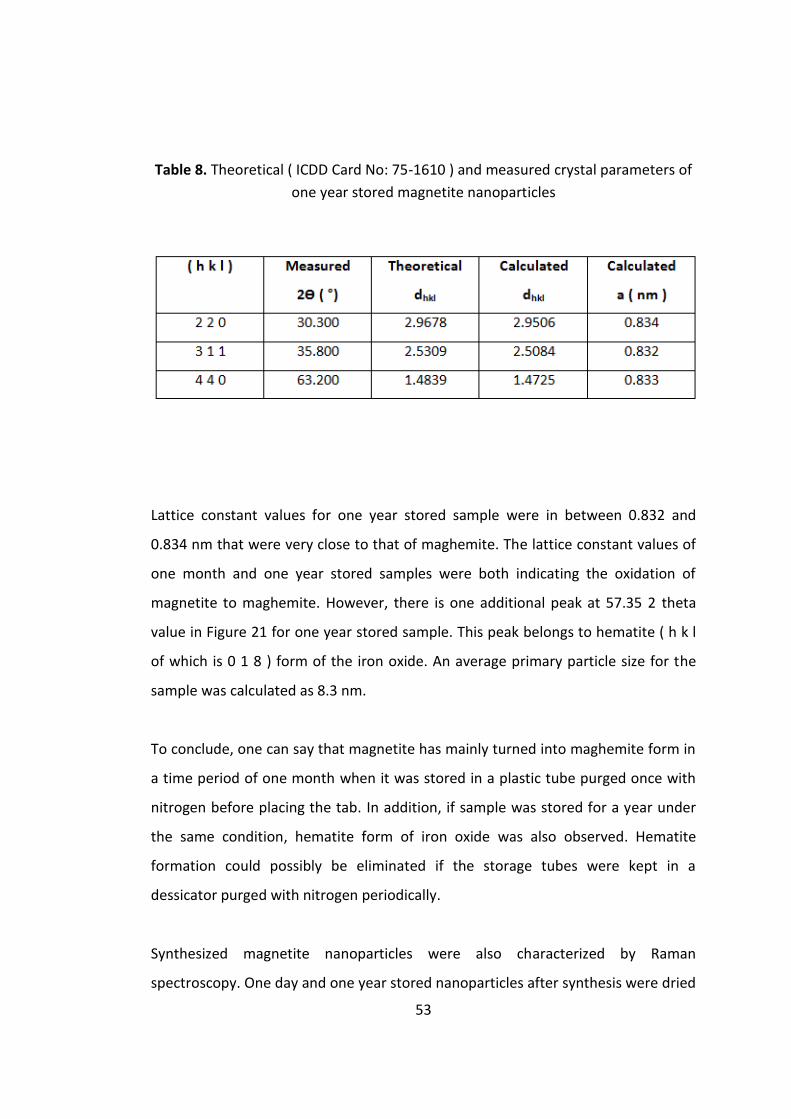
53

Table 8. Theoretical ( ICDD Card No: 75-1610 ) and measured crystal parameters of

one year stored magnetite nanoparticles

Lattice constant values for one year stored sample were in between 0.832 and

0.834 nm that were very close to that of maghemite. The lattice constant values of

one month and one year stored samples were both indicating the oxidation of

magnetite to maghemite. However, there is one additional peak at 57.35 2 theta

value in Figure 21 for one year stored sample. This peak belongs to hematite ( h k l

of which is 0 1 8 ) form of the iron oxide. An average primary particle size for the

sample was calculated as 8.3 nm.

To conclude, one can say that magnetite has mainly turned into maghemite form in

a time period of one month when it was stored in a plastic tube purged once with

nitrogen before placing the tab. In addition, if sample was stored for a year under

the same condition, hematite form of iron oxide was also observed. Hematite

formation could possibly be eliminated if the storage tubes were kept in a

dessicator purged with nitrogen periodically.

Synthesized magnetite nanoparticles were also characterized by Raman

spectroscopy. One day and one year stored nanoparticles after synthesis were dried

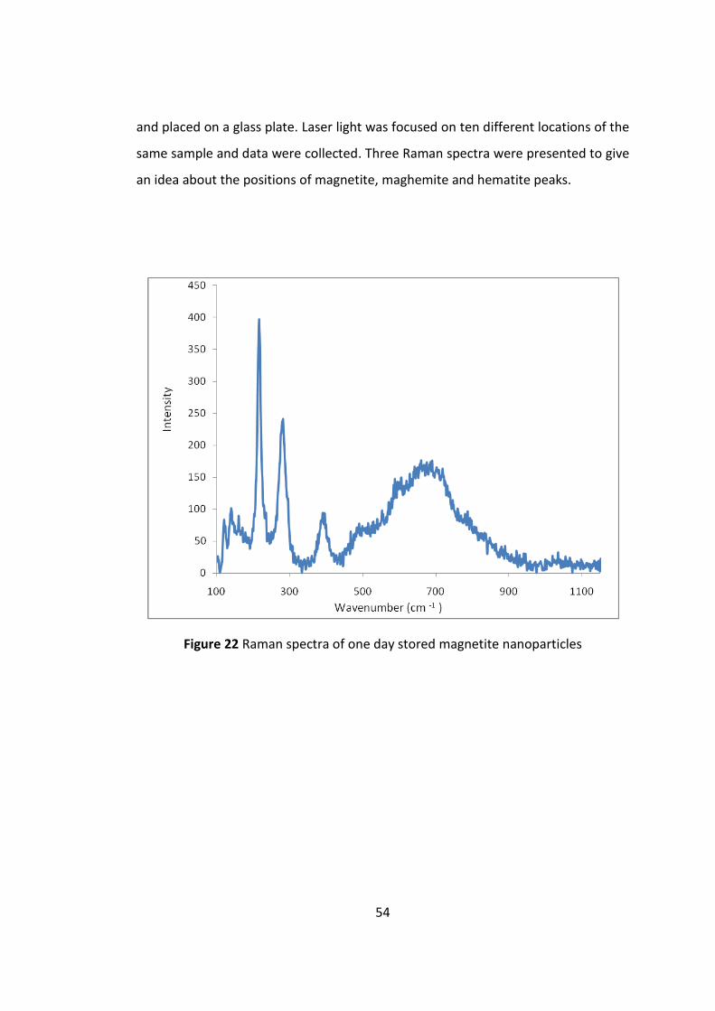
54

and placed on a glass plate. Laser light was focused on ten different locations of the

same sample and data were collected. Three Raman spectra were presented to give

an idea about the positions of magnetite, maghemite and hematite peaks.

Figure 22 Raman spectra of one day stored magnetite nanoparticles

55

Figure 23 Raman spectra of one day stored magnetite nanoparticles

The Raman spectra of one day stored sample were shown in Figure 22. The peaks at

666 cm-1 and at 385 cm -1 were assigned to magnetite and maghemite respectively

whereas the peaks at at 215 and 278 cm-1 were assigned to hematite (Sun, et al.,

2008). It has been stated that the laser power used for the measurement can

change the form of the nanoparticles and may cause thermal broadening and shift

effects (Bersani, Lottici, & Montenero, 1999). We did not observe any hematite

peak from XRD measurements for the samples stored one day, therefore probably

the heat due to laser turned magnetite into hematite form during Raman

measurement.

A Raman spectrum taken from one year stored sample is given in Figure 23.

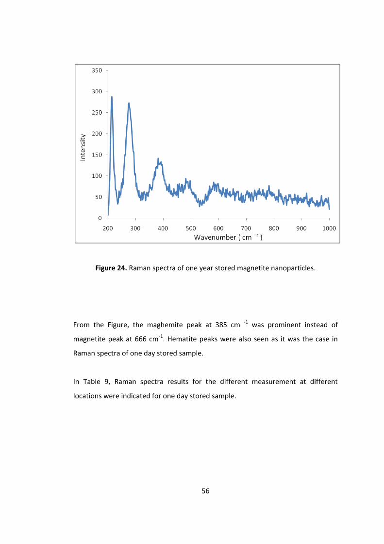
56

Figure 24. Raman spectra of one year stored magnetite nanoparticles.

From the Figure, the maghemite peak at 385 cm -1 was prominent instead of

magnetite peak at 666 cm-1. Hematite peaks were also seen as it was the case in

Raman spectra of one day stored sample.

In Table 9, Raman spectra results for the different measurement at different

locations were indicated for one day stored sample.

57

Table 9. Results of Raman measurements of the one day stored nanoparticles. Ten

different locations of the same sample were investigated.

As can be understood from Table 9, mainly magnetite ( Fe3O4 ) peaks were detected

for the sample stored one day after the synthesis. Only at three positions ( position

# 4, 6, 7) among ten, maghemite ( Ȣ-Fe2O3 ) and hematite (α-Fe2O3 ) form of the iron

oxide were also recorded. The reason of transition into maghemite was the

oxidation during synthesis, drying and measurements. Hematite formation was

probably the case when the sample was exposed enough to the laser radiation of

Raman spectrometry.

In Table 10, Raman spectra results for the different measurement at different

locations were indicated for one year stored sample.

Table 10. Results of Raman measurements of the one year stored nanoparticles

58

One year stored sample were oxidized more compare to the one day stored

sample. Except two locations out of ten (location #, 3 and 8) all three phases,

magnetite, maghemite and hematite were detected. It can be concluded that as the

time passed, maghemite form became dominant in the sample due to oxidation.

In addition to the XRD and Raman results, color of the colloid solutions of samples

stored one day, one month and one year were inspected, as shown in Figure 24.

Magnetite has a black color. When it is oxidized, its color turns into brownish color

of maghemite form. It can be seen from Figure 24 that after one month maghemite

transitions from magnetite took place. In one year time the extend of oxidation was

increased and the color became almost light brown.

Figure 25. Pictures of the magnetite nanoparticle solutions taken at different times

after the synthesis.

59

Since the color of the nanoparticles in solutions may not be identified clearly, the

color of the solid nanoparticles stored at various time intervals were investigated.

For this purpose colloid solutions taken from the vials shown in Figure 24—by

means of a spatula were wiped on a filter paper. The results were shown in Figure

25.

Figure 26. Magnetite nanoparticle solution marked on a paper; a) one day, b) one

month, c) one year stored sample solution

60

Color differences of the solid samples marked on a paper were more easily

identified than their solution form. As presented in Figure 25, one year stored

sample was brown, one month stored sample was deep brown and one day stored

sample was mainly black in color.

The zeta potential values and particle size distributions at various pH values were

measured to find the isoelectric point of the magnetite nanoparticles and to show

particle size distribution trend, as given in Figure 26.

61

Figure 27. The zeta potentials and particle size distributions of magnetite

nanoparticles dispersed at various pH values.

As can be seen from the Figure 26, the isoelectric point of magnetite was found as

7.7 which was in accordance with the literature values (Sun, et al., 2005; Caruso &

Antonietti, 2001). Due to the magnetic dipole attractions, magnetite nanoparticles

tend to aggregate at this neutral pH value and become larger in size. Since

magnetite nanoparticle has the highest positive zeta potential value between pH 2

62

and 4.5, the coulombic repulsion of the magnetic nanoparticles would be enhanced

at this pH range and consequently the magnetic dipole interactions between the

magnetic nanoparticles would be diminished.

The average size of the agglomerated magnetite nanoparticles at pH 2.4 and 8.0

was found around 178 nm from the particle size distribution graphs presented in

Figure 26. However, formation of larger agglomerates ( up to 564 nm ) was

observed at pH 8.0 which was in close proximity of the isoelectric point. Hence the

prepared nanoparticles should be dispersed in aqueous solution at pH values

between 2.0 and 5.0. However, in our studies we were storing them in ethanol.

TEM studies were also conducted to observe the agglomeration of the

nanoparticles and their shape and size. TEM images of the magnetite nanoparticles

are shown in Figure 27.

63

Figure 28. TEM images of magnetite nanoparticles at two different magnifications.

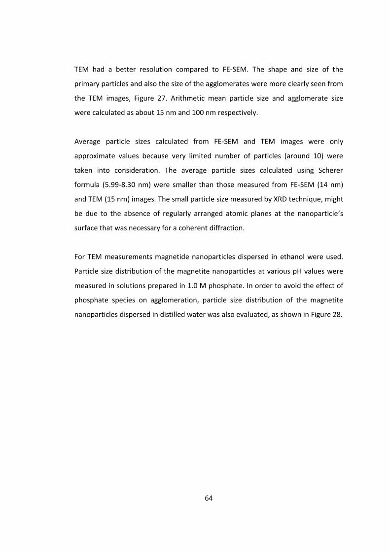
64

TEM had a better resolution compared to FE-SEM. The shape and size of the

primary particles and also the size of the agglomerates were more clearly seen from

the TEM images, Figure 27. Arithmetic mean particle size and agglomerate size

were calculated as about 15 nm and 100 nm respectively.

Average particle sizes calculated from FE-SEM and TEM images were only

approximate values because very limited number of particles (around 10) were

taken into consideration. The average particle sizes calculated using Scherer

formula (5.99-8.30 nm) were smaller than those measured from FE-SEM (14 nm)

and TEM (15 nm) images. The small particle size measured by XRD technique, might

be due to the absence of regularly arranged atomic planes at the nanoparticle’s

surface that was necessary for a coherent diffraction.

For TEM measurements magnetide nanoparticles dispersed in ethanol were used.

Particle size distribution of the magnetite nanoparticles at various pH values were

measured in solutions prepared in 1.0 M phosphate. In order to avoid the effect of

phosphate species on agglomeration, particle size distribution of the magnetite

nanoparticles dispersed in distilled water was also evaluated, as shown in Figure 28.

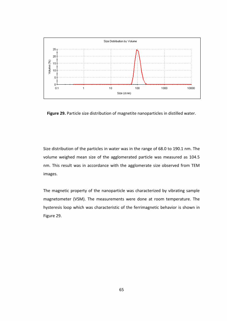
65

Figure 29. Particle size distribution of magnetite nanoparticles in distilled water.

Size distribution of the particles in water was in the range of 68.0 to 190.1 nm. The

volume weighed mean size of the agglomerated particle was measured as 104.5

nm. This result was in accordance with the agglomerate size observed from TEM

images.

The magnetic property of the nanoparticle was characterized by vibrating sample

magnetometer (VSM). The measurements were done at room temperature. The

hysteresis loop which was characteristic of the ferrimagnetic behavior is shown in

Figure 29.

66

Figure 30. Magnetic curve of the magnetite nanoparticles.

For the measurements 0.0156 g and 0.0354 g of magnetite nanoparticles were

taken. The saturation magnetization values of the magnetite nanoparticles were

calculated as 78.82 emu/g for both samples which was in good agreement with the

literature values (Dresco, Zaitsev, Gambino, & Chu, 1999). The covercivity (Hc) of

the nanoparticles was found as 14.2 Oe from the expanded Figure given in Figure

29, inset.

Size is an important factor for magnetic properties. Thus prepared samples were

not superparamagnetic ( at least most of them). Therefore their size should be

larger than 12nm (Tural, Özenbaş, Atalay, & Volkan, 2008). Magnetic

67

measurements also supported the average size of the nanoparticles measured by

TEM and FE-SEM.

3.2 Silica Coating on Magnetite Nanoparticles

Silica coating enhances dispersion properties and diminish toxicity of the

nanoparticles. Besides it provides a platform for further modification of the

nanoparticles with functional groups.

TEOS and APTES were used for silica coating the magnetite nanoparticles. First, 2.5

mM APTES solution was added into the magnetite solution and stirred for a short

time. This enabled amine groups attaching on surface of the nanoparticles. Then,

they were coated with silica by using TEOS with the help of amine groups provided

by APTES. Using small amount of APTES in addition to the TEOS was very important

since better silica coating was obtained compared to the procedure in which only

TEOS was used.

FE-SEM image of the silica coated magnetite nanoparticles was depicted in Figure

30.

68

Figure 31. FE-SEM image of the silica coated magnetite nanoparticles.

From the Figure 30 it can be concluded that nanoparticles were homogeneous in

size and shape. Average particle size of the nanoparticles calculated from the image

was about 40 nm. The difference in the average particle sizes of the magnetite

nanoparticles and silica coated magnetite nanoparticles was attributed to the

thickness of the coated silica layer. Consequently the average thickness should be

about 13 nm.

EDX results of the silica coated nanoparticles are given in Figure 31.

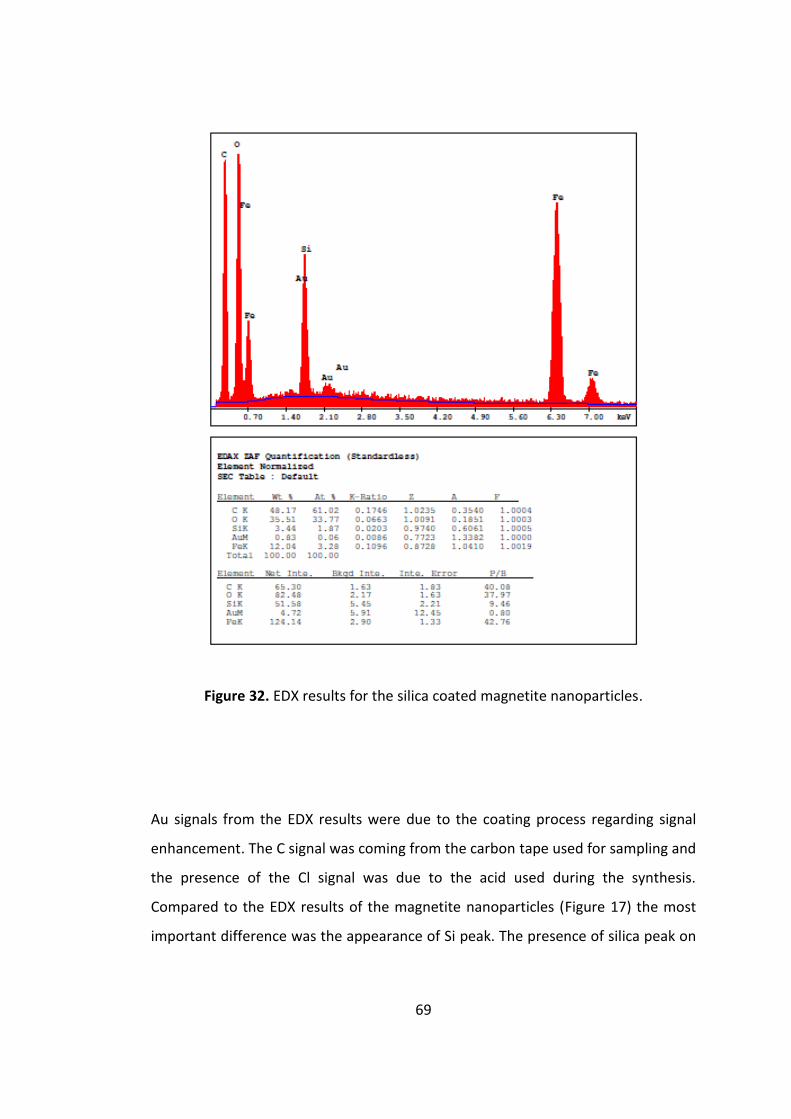
69

Figure 32. EDX results for the silica coated magnetite nanoparticles.

Au signals from the EDX results were due to the coating process regarding signal

enhancement. The C signal was coming from the carbon tape used for sampling and

the presence of the Cl signal was due to the acid used during the synthesis.

Compared to the EDX results of the magnetite nanoparticles (Figure 17) the most

important difference was the appearance of Si peak. The presence of silica peak on

70

the spectrum was considered as the indication of silica layer formation on the

surface of magnetite nanoparticles.

FT-IR analysis was done in order to investigate the bonds concerning the silica layer

formed on magnetite nanoparticle. FT-IR spectrum of this nanoparticles was shown

in Figure 32.

Figure 33. FT-IR spectrum of the silica coated magnetite nanoparticles.

As can be seen from the Figure, in addition to the magnetite peaks, asymmetric and

symmetric stretching of Si-O-Si vibrations were also observed at 1088 cm-1 and 800

71

cm-1 respectively. Their presence was correlated with the coating of silica layer on

magnetite nanoparticles.

Particle size distribution graph of the silica coated magnetite nanoparticles

dispersed in distilled water was measured, as shown in Figure 33.

Figure 34. Particle size distribution of silica coated magnetite nanoparticles in

distilled water.

Size distribution of the particles was in the range of 122.4 and 396.1 nm. Volume

weighed mean size of the agglomerated particles was measured as 221.9 nm.

Isoelectric point of silica is about 2.0. Hence in neutral media, the coulombic

repulsion of the silica coated magnetic nanoparticles should have been enhanced

due to the negative charge of the surface and dispersion would be improved (Sun,

et al., 2005). Quite the opposite to the expectations, the size of the silica coated

magnetite nanoparticle agglomerates was enlarged as compared to the bare

magnetite nanoparticle agglomerates. The possible explanation could be the

72

thickness of the silica layer. It has been stated that the magnetic dipole attraction in

a simplified head to tail configuration is proportional to (r the center distance

of two dipoles). Hence the thickness of the silica shell affects the extend of

attraction (Sun, et al., 2005). Probably the thickness of the coating was not enough

to separate dipoles to a distance at which the attractive forces could be overcame

by repulsive forces of charged surfaces. This fact will be examined further by TEM

and XPS measurements.

3.3 Surface Modification of Magnetite Nanoparticles with APTES

After silica coating of the magnetite nanoparticles, surface modification has taken

the stage. Surface modification by using amino silane was very essential like silica

coating. By attaching functional amine groups onto the surface of the magnetite

nanoparticles, further functional groups and biological compounds could easily be

attached to the surface of the nanoparticles.

FT-IR spectrometer was used for the characterization of the amine groups

introduced on the surface. FT-IR spectrum of the amine modified silica coated

magnetite nanoparticles is shown in Figure 34.

73

Figure 35. FT-IR spectrum of the amine modified silica coated magnetite

nanoparticles

Alkyl C-H stretching and bending vibrations appear at 2850 - 2940 cm-1 and at 1425

cm-1 respectively (He, 2005). Thus the peak at 2939 cm-1 and at 1464 cm-1 were

assigned to –CH2 stretching and bending vibrations respectively. Besides the band

at 882 cm-1 was correlated with the bending vibration of -NH2 group. The existence

of the -CH2 and -NH2 groups on the surface was explained by the attachment of the

APTES on the surface through surface hydroxyl groups. Therefore, it was shown

that the surface of the silica coated magnetite nanoparticles was modified with

APTES. In addition, the absorption band near 3400 cm-1 referred to the vibration of

remainder H2O in the sample.

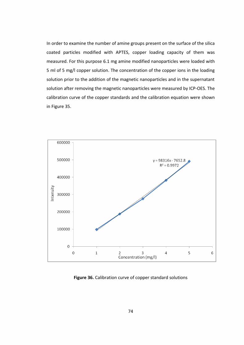
74

In order to examine the number of amine groups present on the surface of the silica

coated particles modified with APTES, copper loading capacity of them was

measured. For this purpose 6.1 mg amine modified nanoparticles were loaded with

5 ml of 5 mg/l copper solution. The concentration of the copper ions in the loading

solution prior to the addition of the magnetic nanoparticles and in the supernatant

solution after removing the magnetic nanoparticles were measured by ICP-OES. The

calibration curve of the copper standards and the calibration equation were shown

in Figure 35.

Figure 36. Calibration curve of copper standard solutions

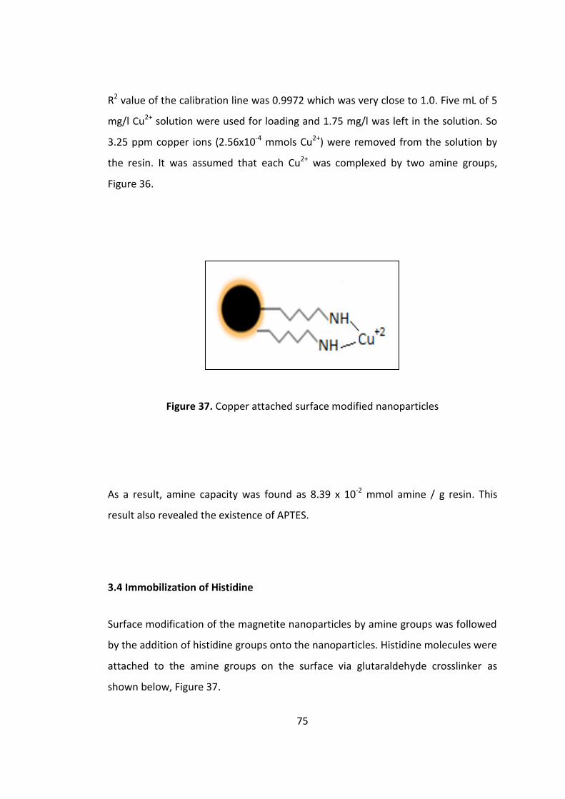
75

R2 value of the calibration line was 0.9972 which was very close to 1.0. Five mL of 5

mg/l Cu2+ solution were used for loading and 1.75 mg/l was left in the solution. So

3.25 ppm copper ions (2.56x10-4 mmols Cu2+) were removed from the solution by

the resin. It was assumed that each Cu2+ was complexed by two amine groups,

Figure 36.

Figure 37. Copper attached surface modified nanoparticles

As a result, amine capacity was found as 8.39 x 10-2 mmol amine / g resin. This

result also revealed the existence of APTES.

3.4 Immobilization of Histidine

Surface modification of the magnetite nanoparticles by amine groups was followed

by the addition of histidine groups onto the nanoparticles. Histidine molecules were

attached to the amine groups on the surface via glutaraldehyde crosslinker as

shown below, Figure 37.

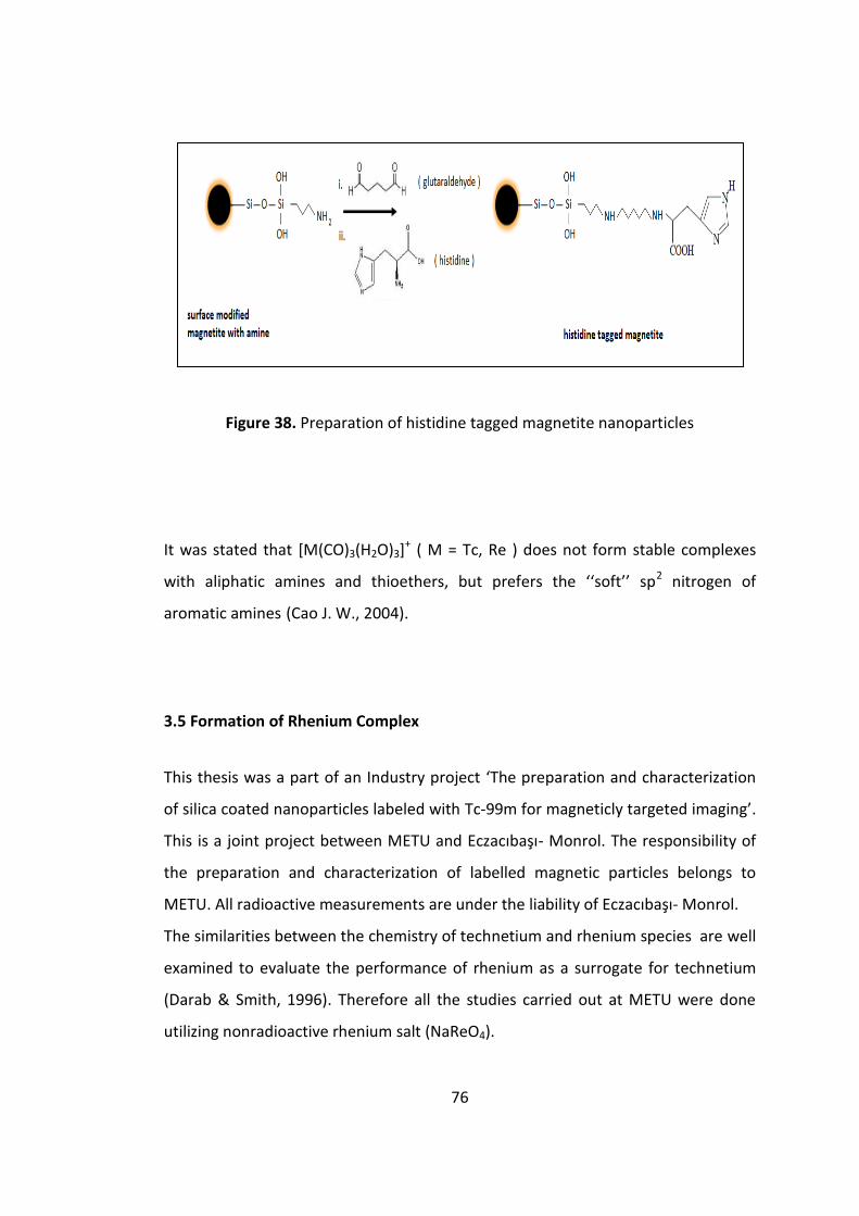
76

Figure 38. Preparation of histidine tagged magnetite nanoparticles

It was stated that [M(CO)3(H2O)3]+ ( M = Tc, Re ) does not form stable complexes

with aliphatic amines and thioethers, but prefers the ‘‘soft’’ sp2 nitrogen of

aromatic amines (Cao J. W., 2004).

3.5 Formation of Rhenium Complex

This thesis was a part of an Industry project ‘The preparation and characterization

of silica coated nanoparticles labeled with Tc-99m for magneticly targeted imaging’.

This is a joint project between METU and Eczacıbaşı- Monrol. The responsibility of

the preparation and characterization of labelled magnetic particles belongs to

METU. All radioactive measurements are under the liability of Eczacıbaşı- Monrol.

The similarities between the chemistry of technetium and rhenium species are well

examined to evaluate the performance of rhenium as a surrogate for technetium

(Darab & Smith, 1996). Therefore all the studies carried out at METU were done

utilizing nonradioactive rhenium salt (NaReO4).

77

Formation of rhenium complex was another important part of this study. Several

biofunctional chelate systems used to link metallic radionuclide to targeting

molecules to give kinetically stable radiopharmaceuticals. The tricarbonyl fragment

M(CO)3+ (M = Tc or Re) is one of them and can be readily produced from

pertechnetate or perrhenate, Figure 38 (Blower, 2006).

Figure 39. Reaction scheme of metal tricarbonyl formation

This process is known as reductive carboxylation. Carbonyl groups are inert, the

labile water ligand can easily be exchanged by a wide variety of tridentate

biofunctional chelators.

Probably rhenium +V and/or +III intermediates are formed during reduction. These

intermediates presumably are stable under neutral/acidic conditions. NaBH4 is

frequently used reducing agent for metal center carbonylation reaction. However it

hydrolyzes fast in acidic medium. Therefore in the carboxylation of Re, NaBH4 is

replaced by water-soluble aminoborane (BH3NH3) which is sufficiently stable under

neutral/acidic conditions and highly reducing (Schibli, 2002).

There are some points that needs to be emphasized for the synthesis of Re carbonyl

complex. First the particle size of the BH3NH3 powder was very important for the

78

complex formation since it was the chemical that holds CO(g). The smaller and well

dispersed the particle of BH3NH3, the more CO(g) will be caught by BH3NH3 by

physical forces during the flushing it with CO(g). Therefore, more CO reacted with

reduced rhenium when smaller and well dispersed BH3NH3, was used. This situation

increased the rhenium complex formation yield directly.

To obtain smaller and well dispersed BH3NH3 particles, it was taken into mortar and

ground well. Then, it was sieved by sieve commonly used in daily life. This was

followed by taking sieved it into a glass vial and flushed with CO(g).

Second was the acidity of the medium. Proper amount, however, of acid should be

chosen to reduce rhenium. In this study 60 µl of H3PO4 were used.

Finally the evolved hydrogen should be controlled. Since reaction of water with

aminoborane brings out hydrogen gas, a syringe must be used to keep the system

pressure balance for safety reasons.

In literature, radioactive rhenium is used in labeling studies. So, the complex

formation efficiency is followed by either thin layer chromatography (TLC) or HPLC

equipped with gamma ray counter. In this study, Re-carbonyl complex and

perrhenate solutions were also run on TLC plate and a UV lamp was used to

visualize the plates together with Eriochrome Black T. (The plate itself contains a

fluorophore which fluoresces everywhere except where an organic compound is on

the plate). However detection of nonradioactive rhenium complex by TLC was not

very successful. Therefore, ICP-MS, a more sensitive technique for rhenium

determination was decided to be used. Rhenium carbonyl complex was separated

from the remaining perrhenate by HPLC and their amounts in the effluent were

measured by ICP-MS.

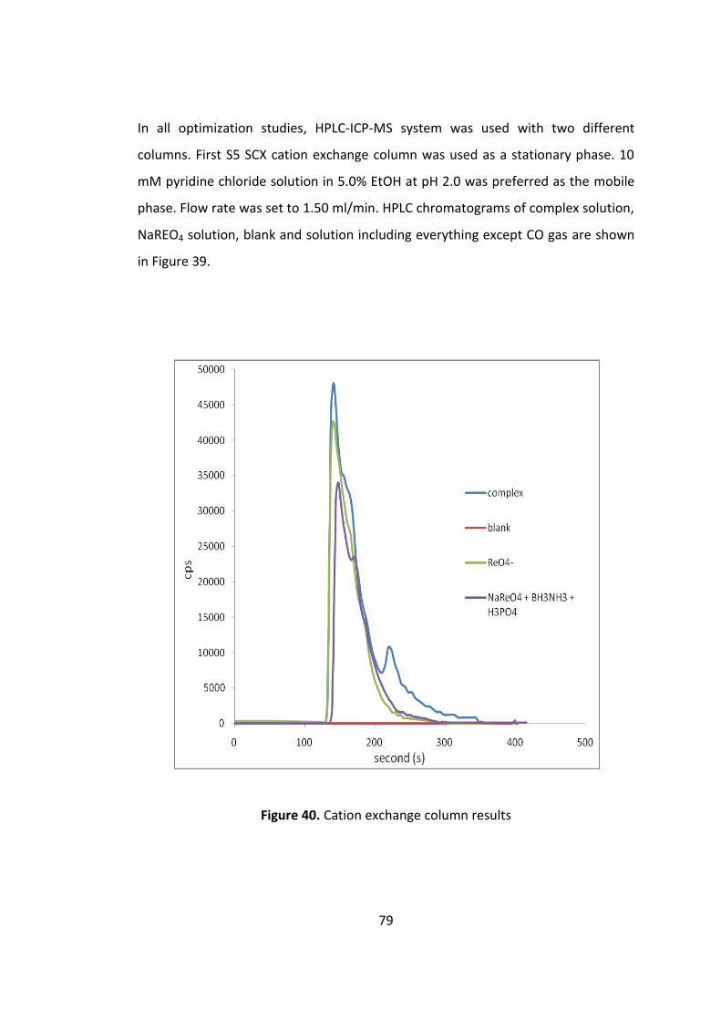
79

In all optimization studies, HPLC-ICP-MS system was used with two different

columns. First S5 SCX cation exchange column was used as a stationary phase. 10

mM pyridine chloride solution in 5.0% EtOH at pH 2.0 was preferred as the mobile

phase. Flow rate was set to 1.50 ml/min. HPLC chromatograms of complex solution,

NaREO4 solution, blank and solution including everything except CO gas are shown

in Figure 39.

Figure 40. Cation exchange column results

80

Since rhenium complex is a positively charged species, it was retained by the cation

exchange column and its signal appeared later than the signal of negatively charged

ReO4- on the chromatogram. As expected ReO4

- standard solution gave just one

peak. Whereas blank solution that did not have any rhenium gave no signal. A

solution which included ReO4- together with BH3NH3 and H3PO4 but not purged with

CO(g) gave the same signal as ReO4- alone. This means that rhenium after reduced in

acidic medium gave reaction only in the presence of carbon monoxide in the

medium.

After showing the rhenium complex formation, S5 SAX anion exchange column was

also used as a stationary phase for obtaining a better signal separation. 5mM

sodium citrate solution in 10.0% MeOH at pH 4.5 was used as the mobile phase.

The same flow rate was preferred as 1.50 ml/min. HPLC chromatogram is shown in

Figure 40.

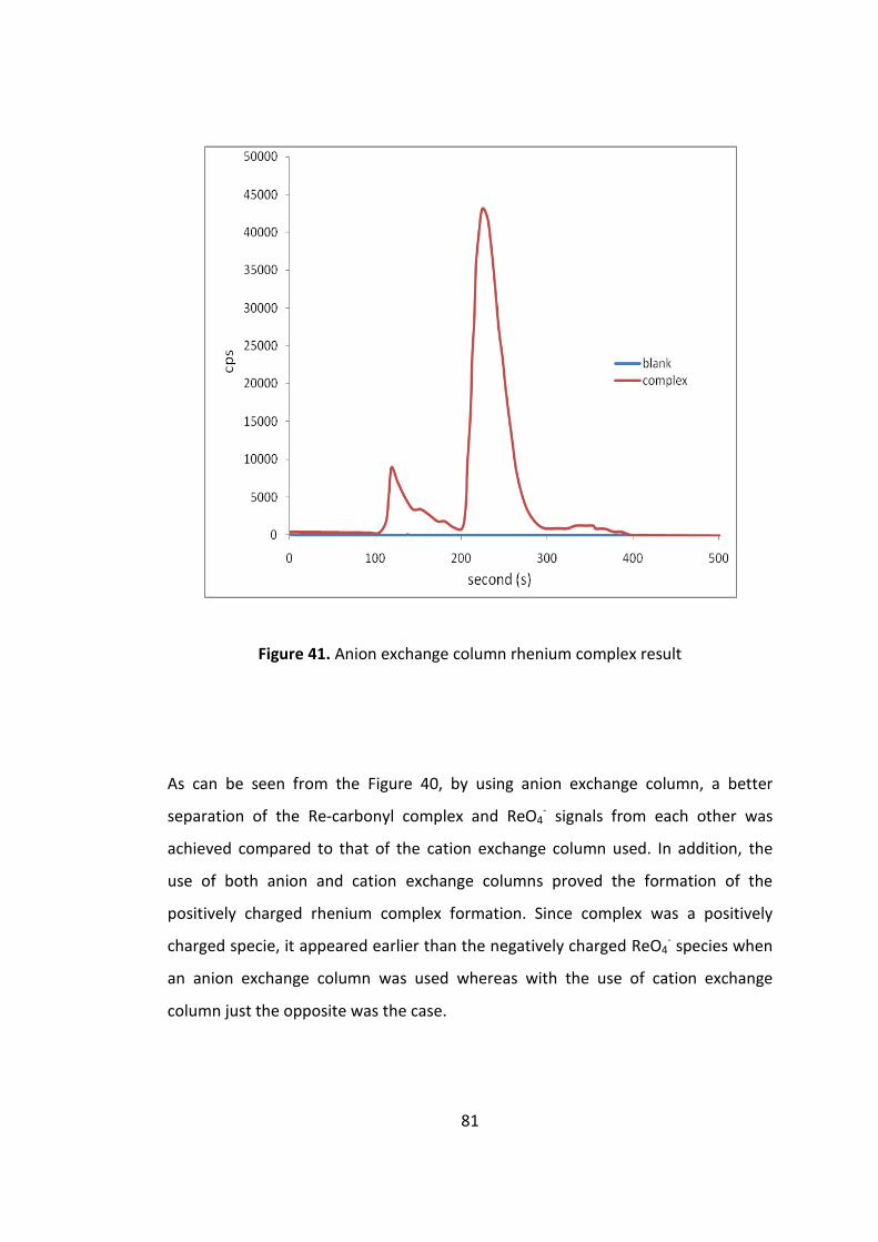
81

Figure 41. Anion exchange column rhenium complex result

As can be seen from the Figure 40, by using anion exchange column, a better

separation of the Re-carbonyl complex and ReO4- signals from each other was

achieved compared to that of the cation exchange column used. In addition, the

use of both anion and cation exchange columns proved the formation of the

positively charged rhenium complex formation. Since complex was a positively

charged specie, it appeared earlier than the negatively charged ReO4- species when

an anion exchange column was used whereas with the use of cation exchange

column just the opposite was the case.

82

At the beginning of the study, complex formation yield was not high enough since

large amount of the ReO4- remained unreacted, Figure 40. First phosphoric acid

volume was increased from 30 to 60 µl and complex formation yield was improved

to around % 28. Then, type of vial was changed. CO(g) was one of the reactant of the

complex formation reaction. Hence, the saturation of the medium with CO

throughout the reaction period should be an important parameter to be controlled.

Therefore, a gas-tight vial was used to prevent the leakage of CO gas. Moreover, in

order to enhance the interaction between the gas and the solid reagent, the

particle size of aminoborane powder was reduced and the mixture was agitated

using a stirring bar. For this purpose, aminoborane solid was ground and sieved

before use and the reaction was carried out on a magnetic stirrer. Finally, a desired

complex formation yield (more than 90%) was reached which was shown in Figure

41.

83

Figure 42. HPLC (anion exchange column )- MS chromatogram of the rhenium

complex prepared at optimized conditions.

As can be seen from the Figure 41, almost all perrhenate was taken into the

complex and only a small amount of ReO4- was left in the solution. The complex

formation yield was calculated by finding the percent ratio of the peak area of the

complex to the total area of the peaks. Hence, the areas under the peaks and the

total area were measured by using software of the HPLC instrument and complex

formation yield was found around 95% at the optimized conditions.

84

Another parameter that was investigated was the duration of CO gas flushing.

During optimization studies, CO gas purging period had been kept as 80 minutes, so

shorter duration times were tried. Complex formation yields corresponding to the

various duration times (5, 10 and 80 minutes) of CO gas flushing were presented in

Figure 42.

Figure 43. Complex formation yields at different CO gas flushing times

As can be seen from the Figure 42, the complex formation yields are similar (around

90 %) at the CO gas flushing time of 10 and 80 minutes, whereas it declines at a gas

flushing time of 5 min. In order to consume less gas, 10 minutes were chosen as a

proper period for saturating the solid reducing agent (amino borane, 10mg) with CO

gas. For Re-carbonyl complex formation studies the same (or the same type of) vial

was used throughout the study with the optimized conditions.

85

In addition, the stability of the rhenium complex during storage was examined. It

was stated that the carbonyl complex is unstable unless taken into a chelate and

turns into perrhenate again in a day (Schibli, 2002). For this purpose the HPLC-MS

chromatograms of the Re-carbonyl complex were taken directly following the

preparation, after one day and one week. In contrast to the literature (Schibli,

2002) thus prepared rhenium complex was stable after one day and even in one

weak time (Schibli, 2002).

3.6. Labeling of Histidine-immobilized Nanoparticles with Rhenium Complex

Labeling the nanoparticles with rhenium complex plays very important role in this

study. The attachment of Re/Tc carbonyl complexes on the surface of nanoparticles

through histidine groups was depicted in schematic representation below, Figure

43.

Figure 44. Nanoparticle labelled with Re-carbonyl complex via histidine group

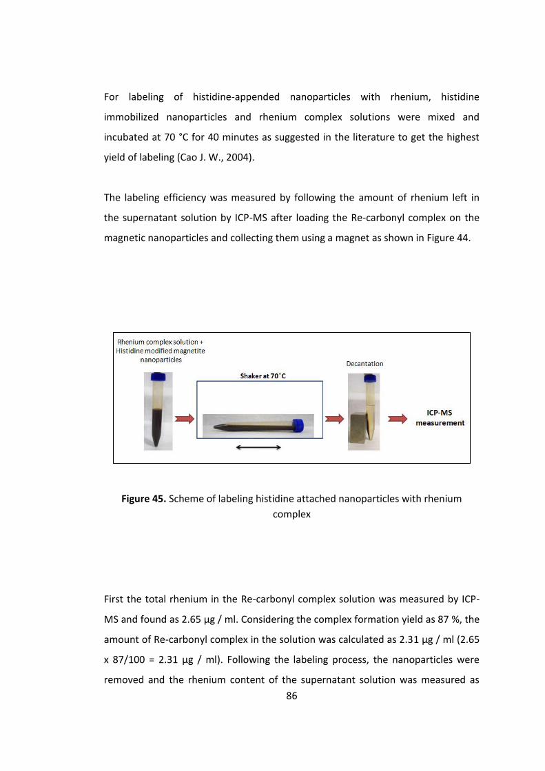
86

For labeling of histidine-appended nanoparticles with rhenium, histidine

immobilized nanoparticles and rhenium complex solutions were mixed and

incubated at 70 °C for 40 minutes as suggested in the literature to get the highest

yield of labeling (Cao J. W., 2004).

The labeling efficiency was measured by following the amount of rhenium left in

the supernatant solution by ICP-MS after loading the Re-carbonyl complex on the

magnetic nanoparticles and collecting them using a magnet as shown in Figure 44.

Figure 45. Scheme of labeling histidine attached nanoparticles with rhenium

complex

First the total rhenium in the Re-carbonyl complex solution was measured by ICP-

MS and found as 2.65 µg / ml. Considering the complex formation yield as 87 %, the

amount of Re-carbonyl complex in the solution was calculated as 2.31 µg / ml (2.65

x 87/100 = 2.31 µg / ml). Following the labeling process, the nanoparticles were

removed and the rhenium content of the supernatant solution was measured as

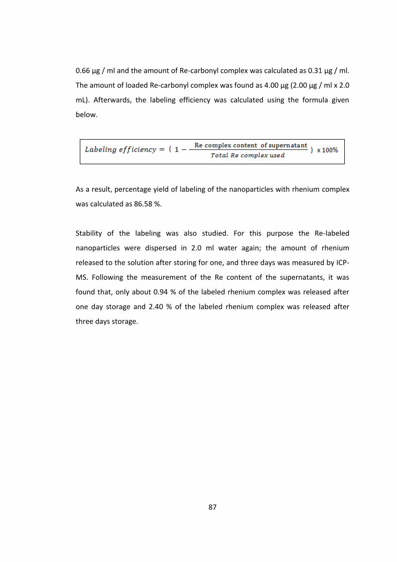
87

0.66 µg / ml and the amount of Re-carbonyl complex was calculated as 0.31 µg / ml.

The amount of loaded Re-carbonyl complex was found as 4.00 µg (2.00 µg / ml x 2.0

mL). Afterwards, the labeling efficiency was calculated using the formula given

below.

As a result, percentage yield of labeling of the nanoparticles with rhenium complex

was calculated as 86.58 %.

Stability of the labeling was also studied. For this purpose the Re-labeled

nanoparticles were dispersed in 2.0 ml water again; the amount of rhenium

released to the solution after storing for one, and three days was measured by ICP-

MS. Following the measurement of the Re content of the supernatants, it was

found that, only about 0.94 % of the labeled rhenium complex was released after

one day storage and 2.40 % of the labeled rhenium complex was released after

three days storage.

88

CHAPTER 4

CONCLUSION

Molecular imaging and radiotherapy using radionuclides is a rapidly expanding field

of medicine and medical research. Magnetic nanoparticles have been proposed for

use as biomedical purposes to a large extent for several years. In recent years,

nanotechnology has developed to a stage that makes it possible to produce,

characterize and specifically tailor the functional properties of nanoparticles for

clinical applications. A potential benefit of using magnetic nanoparticles in

biomedical studies is the use of localized magnetic field gradients to target the

particles to a chosen site, to hold them there until the therapy is complete and then

to remove them.

This thesis was a part of an industrial project ‘The preparation and characterization

of silica coated nanoparticles labeled with Tc-99m for magneticly targeted imaging’

This is a joint project between METU and Eczacıbaşı- Monrol. The responsibility of

the preparation and chacterization of labeled magnetic particles belongs to METU.

Due to the similarities between the chemistry of technetium and rhenium species,

all the studies carried out at METU were done utilizing nanradioactive rhenium salt

(NaReO4).

In this study, magnetic iron oxide nanoparticles, magnetite, were synthesized by

coprecipitation method. According to this method, Iron (II) and iron (III) salts were

precipitated by adding a base, ammonia solution, to obtain nanoparticles. The

average particle size of magnetite nanoparticles was calculated as 15 nm. The

morphology, size and magnetic properties of the nanoparticles were characterized

by FE-SEM, TEM, EDX, XRD and VSM.

89

Magnetite nanoparticles were coated with silica to improve biocompability and to

establish a platform for further modification, mainly. APTES and TEOS were the

silica precursors. FE-SEM images, EDX analysis and FT-IR measurements were taken

to indicate the silica coating. From the FE-SEM images average particle size of the

silica coated nanoparticles was calculated as 40 nm.

Silanization of nanoparticles was another required step in this study to be able to

create a nanoparticle having amine modified surface for further functional group

attachment studies. APTES was used during the silanization. FT-IR measurements

were taken for characterization of these nanoparticles. In addition, ICP-OES

measurements were done in order to estimate the number of amine groups

present on the surface (amine capacity) through copper loading experiments. The

amine capacity of amine modified nanoparticles was found as 8.39 x 10-2 mmol

amine / g resin.

Histidine was immobilized onto the surface of the amine modified nanoparticles to

capture the label. with rhenium complex, Instead of radioactive technetium, non-

radioactive rhenium as a surrogate was preferred to use in our studies due to safety

reasons. Rhenium complex [Re(CO)3(H2O)3]+ was synthesized through reaction of

NaReO4 with CO gas in an acidic and reducing medium. By HPLC-ICP-MS

measurements the complex formation yield was calculated as 95% . The stability of

labeled particles was evaluated by ICP-OES measurements of the rhenium released

to the aqueous solution of the labeled nanoparticles.

90

REFERENCES

Allison, W. (2006). Fundamental Physics for Probing and Imaging. United States:

Oxford University Press Inc.

Babes, L., Denizot, B., Tanguy, G., Jacques, J., Jeune, L., & Jallet, P. (1999). Journal of

Colloid and Interface Science , 212, 474.

Bersani, D., Lottici, P. P., & Montenero, A. (1999). Journal of Raman Spectroscopy ,

30, 355.

Blower, P. (2006). Dalton Transactions , 1705.

Boisseau, P., Houdy, P., & Lahmani, M. (2007). Nanoscience: Nanobiotechnology

and Nanobiology. France: Springer Verlag .

Bruce, J. I., & Sen, T. (2005). Langmuir , 21, 7029.

Cao, G., Zhang, Q., & Brinker, J. C. (2010). Annual review of Nano Research, Vol. 3 .

Singapore: World Scientific Publishing Co. Pte. Ltd.

Cao, J. W. (2004). Journal of Magnetism and Magnetic Materials , 277, 165-174.

Caruso, A. R., & Antonietti, M. (2001). Cmemistry of Materials , 13, 3272.

Chastellain, M., Petri, A., Gupta, A., Rao, K. V., & Hofmann, H. (2004). Advanced

Engineering Materials , 6, 235.

Choppin, R. G., Liljenzin, J., & Rydberg, J. (2002). Radiochemistry and Nuclear

Chemistry. United States of America: Butterworth-Heinemann.

Çorman, E. M., Öztürk, N., Bereli, N., Akgöl, S., Denizli, & A. (2010). Journal of

Molecular Catalysis B: Enzymatic , 63, 102.

Cornell, M. R., & Schwertmann, U. (2003). The iron oxides: structure, properties,

recations, occurences, and uses. Germany: WILEY-VCH Verlag GmbH Co.KGaA.

Culita, D. C., Gabriela, M., Patron, L., Carp, O., Cizmas, B. C., & Diamandescu, L.

(2008). Materials Chemistry and Physics. 111, 381.

Curtis, A. S., & Wilkinson, C. (2001). 19, 97-101.

91

Darab, G. R., & Smith, A. P. (1996). Chemistry of Materials , 8, 1004.

Deng, Y., Wang, C., Hu, J., Yang, W., & Fu, S. (2005). Colloids and Surfaces A:

Physicochemical and Engineering Aspects , 262, 87.

Dilworth, R. J., & Parrott, J. S. (1998). Chemical Society Reviews , 27, 43.

Dionnei, G. (2009). Magnetic Oxides. London: Springer Science+Business Media.

Dresco, A. P., Zaitsev, S. V., Gambino, J. R., & Chu, B. (1999). Langmuir , 15, 1945.

Fendler, H. J., & Dekany, I. (1996). Nanoparticles in Solids and Solutions.

Netherlands: Kluwer Academic Publishers.

Friedlander, G. (2008). Introduction to Radiochemistry . United States of America:

John Wiley & Sons, Inc.

Gonser, W. B. (1962). Rhenium. The Netherlands: Elsevier Publishing Company.

Gossuin, Y., Gillis, P., A., H., Vuong, L. Q., & Roch, A. (2009). Nanomedicine and

Nanobiotechnology , 1, 299.

Greg Goebel. (n.d.). Retrieved from www.vectorsite.net

Gubin, P. S. (2009). Magnetic Nanoparticles. Weinheim: WILEY VCH Verkab GmbH &

Co.

Gupta, A. K., & Gupta, M. (2005). Biomaterials , 26, 3995.

Gupta, K. A., & Wells, S. (2004). IEEE Transactions on Nanobiosicience , 3, 66.

Hafeli, U., Gayle Pauer, G., Failing, S., & Tapolsky, G. (2001). Journal of Magnetism

and Magnetic Materials , 225, 73.

Hafeli, U., Pauer, G., Failing, S., & Tapolsky, G. (2001). Journal of Magnetism and

Magnetic Materials.

Hamoudeh, M., Kamleh, A. M., Diab, R., & Fessi, H. (2008). Advanced Drug Delivery

Reviews , 60, 1329.

Hamoudeh, M., Salim, H., Barbos, D., Paunoiu, C., & Fessi, H. (2007). European

Journal of Pharmaceutics and Biopharmaceutics , 67, 597.

He, P. Y. (2005). JournalL Of Physics D: Applied Physics , 38, 1342.

Herdt, R. A., Kim, B., & Taton, A. T. (2007). Bioconjugate Chemistry. 18, 183.

92

Hu, A., Salabas, L. E., & Schüth, F. (2007). Angewantde Chemie , 46, 1222.

Jarrett, R. B., Gustafsson, B., Kukis, L. D., & Louie, Y. A. (2008). Bioconjugate

Chemistry , 19, 1496.

Kairemo, K., Erba, P., Bergström, K., & Pauwels, K. J. (2008). Current

Radiopharmaceuticals. 1, 30.

Karlsson, A. N., Deppert, K., Karlsson, L., & Malm, J. (2005). Applied Physics A:

Materials Science and Processing , 80, 1579.

Kelsall, W. R., Hamley, W. I., & Geoghegan, M. (2005). Nanoscale Science and

Technology . England: John Wiley & Sons Ltd. .

Kröger, D., Liley, M., Schiweck, W., Skerra, A., & Vogel, H. (1999). Biosensors &

Bioelectronics , 14, 155.

Kumar, C. (2009). Magnetic Nanomaterials. Germany: WILEY-VCH Verlab GmbH &

Co.

Kwei, G. H., von Dreele, R. B., Williams, A., Goldstone, J. A., Lawson, A. C., &

Warburton, W. K. (1990). Journal of Molecular Structure , 223, 383-406.

Laurent, S., Forge, D., Port, M., Roch, A., Robic, C., Elst, V. L., et al. (2008). Chemical

Revieews , 108, 2064.

Lebedev, B. K. (1962). The Chemistry of Rhenium. Great Britain: Butterworth & Co.

(Publishers) Ltd.

Liang, S., Wang, Y., yu, J., Zhang, C., Xia, J., & Yin, D. (2007). Journal of Materials

Science: Materials in Medicine , 18, 2297.

Lim, T. Y., Lee, Y. K., Lee, K., & Chung, H. B. (2006). Biochemical and Biophysical

Research Communications , 344, 926.

Liu, Z., Zu, Y., Fu, Y., Meng, R., Guo, S., Xing, Z., et al. (2010). Colloids and Surfaces B:

Biointerfaces , 76, 311.

Liz-Marzan, M. L. (1996). Langmuir , 12, 4329-4335.

Liz-Marzan, M. L. (2003). Nanoscale Materials. United States of Anerica: Kluwer

Academic Publishers.

Lu, A., Salabas, L. E., & Schüth, F. (2007). Angewandte Chemie International Edition ,

46, 1222.

93

Lu, Y., Yin, Y., Mayers, T. B., & Xia, Y. (2002). Nano Letters , 2, 183.

Lucignani, G., Ottobrini, L., Martelli, C., Rescigno, M., & Clerici, M. (2006). Trends in

Biotechnology , 24, 410.

Lue, J. (2001). Journal of Physics and Chemistry of Solids , 62, 1599.

Ma, D., Guan, J., Normandin, F., Denommee, S., Enright, G., Veres, T., et al. (2006).

Chemistry of Materials . 18, 1920.

Ma, M. Z. (2003). 212, 219-226.

Ma, M., Zhang, Y., Yu, W., Shen, H., Zhang, H., & Gu, N. (2003). Colloids and Surfaces

A: Physicochemistry Engineering Aspects , 212, 219.

Ma, Z., Guan, Y., & Liu, H. (2006). Journal of Magnetism and Magnetic Materials ,

301, 469.

Martinez, B., Roig, A., Molins, E., Gonzalez-Carreno, T., & Serna, J. C. (1998). Journal

of Applied Physics , 83, 3256.

Mineralogy Database, www.mindat.org, last visited on November 2010

Moghimi, M. S., Hunter, A. C., & Murray, J. C. (2001). 53, 283-318.

Molday, R. S. (1984). Patent No. 4452773. US Patent.

Morales, P. M., Gonzalez-Carreno, T., Ocana, M., Alonso-Sanudo, M., & Serna, J. C.

(2000). Journal of Solid State Chemistry , 155, 458.

Morel, A., Nikitenko, I. S., Gionnet, K., Wattiaux, A., Lai-Kee-Him, J., Labrugere, C., et

al. (2008). ACS Nano , 2, 847.

Najariani, K., & Splinter, R. (2006). Biomedical Signal and Image Process. United

Statees of America: Taylor & Francis Group, LLC.

Ottobrini, L., Ciana, P., Biserni, A., Lucignani, G., & Maggi, A. (2006). Molecular and

Cellular Endocrinology , 246, 69.

Pankhurst, A. Q., Connolly, J., S., J. K., & J., D. (2003). 36, R167–R181.

Panyam, J., & Labhasetwar, V. (2003). Advanced Drug Delivery Reviews , 55, 329.

Peacock, D. R. (1966). The Chemistry of Technetium and Rhenium. The Netherlands:

Elsevier Publishing Company.

94

Reimer, L., & Kohl, H. (2008). Transmission Electron Microscopy: Physics of Image

Formation . Germany: Springer.

Schibli, R. S. (2002). Bioconjugate Chemistry , 13, 750.

Schmid, G. (2010). Nanoparticles: From Theory to Application. Germnay: WILEY-VCH

Verlag GmbH Co. KGaA.

Schwertmann, U., & Cornell, M. R. (2000). Iron oxides in the laboratory: preparation

and characterization. Germany: WILEY-VHC Verlag GmbH.

Sergeev, B. G. (2006). Nanochemistry. The Netherlands: Elsevier B. V.

Shirley, H. J., & Fairbridge, W. R. (1997). Encyclopedia of planetary sciences. London:

Chapman & Hall.

Spinks, T. W., & Woods, J. R. (1976). An Introduction to Radiation Chemistry.

Canada: John Wiley &n Sons, Inc.

Stichelberger, M., Desbouis, D., Spiwok, V., Scapozza, L., Schubiger, A. P., & Schibli,

R. (2007). Journal of Organometallic Chemistry , 692, 1255.

Sun, L., Y., H., Chien, C. L., & Searson, P. C. (2005). IBM Journal of Reserach and

Development , 49, 79.

Sun, X., Zheng, C., Zhang, F., Li, L., Yang, Y., Wu, G., et al. (2008). The Journal of

Physical Chemistry C , 12, 17148.

Sun, Y., Duan, L., Guo, Z., DuanMu, Y., Ma, M., Xu, L., et al. (2005). Journal of

Magnetism and Magnetic Materials , 285, 65.

Suryanarayana, C., & Norton, G. M. (1998). X-Ray Diffraction: A Practical Approach.

United States of America: Plenum Press.

Swihart, T. M. (2003). Current Opinion in Colloid and Interface Science , 8, 127.

Tartaj, P., Gonzalez-Carreno, T., Rebolledo, F. A., Bomati-Miguel, O., & Serna, J. C.

(2007). Journal of Colloid and Interface Science , 309, 68.

Thomas, S., & Stephen, R. (2010). Rubber Nanocomposites: Preparation, Properties

and Applications. Singapore: John Wiley and Sons (Asia)Pte. Ltd.

Thorek, J. L., Chien, K. A., Czupryna, J., & Tsourkas, A. (2006). Annals of Biomedical

Engineering , 34, 23.

95

Tural, B., Özenbaş, M., Atalay, S., & Volkan, M. (2008). Journal of Nanoscience and

Nanotechnology , 8, 861.

Turner, E. J. (2007). Atoms, Radiation and Radiation Protection. Germany: WILEY-

VCH Verlag GmbH Co. KGaA.

Varadan, K. V. (2008). Nanomedicine: design and applications of magnetic

nanomaterials, nanosensors, and nanosystems . United Kingdom: John Wiley &

Sons, Ltd.

Volath, D. (2008). Nanomaterials: An Introduction to Synthesis, Properties and

Application. Germany: WILEY-VCH Verlab GmbH & Co.

Waibel, R., Alberto, R., Willuda, J., Finnern, R., Schibli, R., Stichelberger, A., et al.

(1999). Nature Biotechnology , 17, 897.

Wilkinson, J. M. (2003). Medical Device Technology , 14, 29.

Wunderlich, G., Pinkert, J., Andreeff, M., Stintz, M., Knapp Jr, F. F., Kropp, J., et al.

(2000). Applied Radiation and Isotopes , 52, 63.

Zhao, L., Zhang, H., Xing, Y., Song, S., Yu, S., Shi, W., et al. (2007). Chemistry of

Materials , 20, 198.