PREMIA FOR CORRELATED DEFAULT RISK

Shahriar Azizpour∗

Stanford University

Kay Giesecke†

Stanford University

January 28, 2008; this draft June 26, 2008‡

Abstract

Credit investors are exposed to correlated changes in issuers’ conditional defaultrates that are due to movements in common risk factors, and the feedback jumpsin default rates that are caused by the impact of a default event on the survivingfirms. This article explores the risk premia investors require for bearing that expo-sure during April 2004–October 2007. We develop and estimate from an extensivedata set of corporate defaults and market rates of CDX High Yield and InvestmentGrade index and tranche swaps a reduced-form model of correlated firm defaultunder actual and risk-neutral probabilities. Our likelihood estimators indicate thatCDX investors require substantial premia for the diffusive mark-to-market risk thatis caused by firms’ common factor exposure, and the jump-to-default risk in swapvalues that comes from the impact of an event on the portfolio constituents. Riskpremia vary dramatically across time, portfolio composition, and holding period.

Key words: Correlated default, feedback, intensity, risk premia, measure change,pricing kernel.

∗Department of Management Science & Engineering, Stanford University, Stanford, CA 94305-4026,USA, email: azizpour@stanford.edu†Department of Management Science & Engineering, Stanford University, Stanford, CA 94305-

4026, USA, Phone (650) 723 9265, Fax (650) 723 1614, email: giesecke@stanford.edu, web:www.stanford.edu/∼giesecke.‡This research was supported by grants from JP Morgan Chase’s Academic Outreach Program and

Moody’s Credit Market Research Fund, for which we are very grateful. We are also grateful for data fromBarclays Capital and Moody’s Investors Service. We thank Sanjiv Das, Andreas Eckner, Eymen Errais,Francis Longstaff, Ilya Strebulaev, Stefan Weber, Liuren Wu and seminar participants at the Universityof Chicago’s Stevanovich Center for Financial Mathematics Conference on Credit Risk, the Standardand Poor’s Credit Risk Summit and the Daiwa International Workshop on Financial Engineering fordiscussions and comments, and Baeho Kim and Wilfred Wong for excellent research assistance.

1

1 Introduction

Corporate defaults cluster. This article develops a reduced-form model of the term struc-

ture of correlated default risk under actual and risk-neutral probabilities, and estimates

the time-series, cross-sectional and term-structure behavior of the premia for clustered cor-

porate default risk during April 2004–October 2007. The analysis is based on a database

of nearly 1400 default incidences, and market rates of index and tranche swaps referenced

on the CDX High Yield and Investment Grade portfolios of North American issuers. The

swap rates cover the entire trading history through October 2007 of High Yield and In-

vestment Grade contracts of all maturities. They offer a unique opportunity for extracting

investors’ risk-neutral probabilities of joint default.

According to our pricing model, defaults are correlated because firms are exposed to

a square-root diffusion risk factor, and because a default has an impact on the surviv-

ing firms that is channeled through the complex web of legal, business and informational

relationships in the economy. This specification accommodates the feedback phenomena

that are often observed in credit markets.1 Our maximum likelihood estimators indicate

that feedback effects induce jump risks that are of significant concern to credit investors,

and that are priced into the CDX index and tranche swap market. A default is estimated

to have a substantial, highly persistent impact on swap rates. Because of this influence,

correlated default risk is not conditionally diversifiable as in the doubly-stochastic econ-

omy of Jarrow, Lando & Yu (2005). A default event may command a premium even in

well-diversified portfolios of credit-sensitive positions.

We find that CDX index and tranche investors require substantial compensation

for bearing exposure to correlated jump-to-default risk and non-default mark-to-market

risk. Non-default mark-to-market risk relates to the diffusive variation in swap market

rates. It is due to firms’ exposure to a common risk factor, whose diffusive movements

induce correlated changes in firms’ conditional default probabilities. Jump-to-default risk

relates to the abrupt changes in index and tranche market rates at defaults. The jumps in

market rates reflect the feedback from events and the associated adjustment of the mark-

to-market values of the surviving portfolio constituent swaps. Our estimators indicate

that this adjustment risk is economically important, and that it is priced into the CDX

market. The total compensation for time-variation (diffusive and jump) in swap market

rates is higher for the High Yield portfolio of low-quality issuers.

Jump-to-default risk premia vary dramatically over time, and are much higher and

much more volatile for the Investment Grade portfolio of high-quality firms. During the

second quarter of 2005, jump-to-default premia increased quickly to peak in May 2005,

1For example, Lang & Stulz (1992) and Jorion & Zhang (2007b) find that intra-industry contagion isoften associated with Chapter 11 bankruptcies. Collin-Dufresne, Goldstein & Helwege (2003) show thatcredit events of large firms generate a market-wide response in credit spreads. Jorion & Zhang (2007a)find that a firm’s default leads to abnormally negative equity returns for the firm’s creditors along withsignificant increases in creditors’ credit swap spreads.

2

marking the height of the correlation crisis that is often linked to the downgrades of Ford

and General Motors. They spiked again in September 2006, and then steadily declined,

reaching almost zero in late February 2007. From this trough, jump-to-default premia

surged rapidly to peak in early August 2007 at historically extreme levels, reflecting the

growing concern about a serious credit crisis in the U.S. due to strings of mortgage defaults,

and the spread of that crisis to the corporate credit market. Corporate credit investors

sought cover in the CDX market at any price, while corporate default rates remained

historically low. Jump-to-default premia declined somewhat from their extreme levels but

remained relatively high through October 2007.

Our model of clustered event timing is formulated in terms of a portfolio default

intensity, which represents the conditional default rate in a portfolio of correlated issuers.

This top-down perspective allows us to parsimoniously describe the salient empirical char-

acteristics of default clustering, including common factor exposure and feedback. It also

allows us to capture the negative correlation between default and recovery rates that is

well-documented empirically. Further, the top-down approach leads to (semi-) analytic

valuation relations for index and tranche swaps, as well as computationally tractable

maximum likelihood estimation of the model parameters. Our methodology enables us to

empirically disentangle the effects of correlated default risk on index and tranche swap

rates, and to measure the premia associated with these effects.

The presence of jump-to-default premia implies that the portfolio intensity follows

distinct stochastic processes under actual and risk-neutral measures. The behavior of the

actual portfolio intensity is estimated from corporate default experience in the universe of

Moodys rated issuers. The dynamics of the risk-neutral intensity under actual and risk-

neutral probabilities are estimated from time series of CDX index and tranche swap market

rates for several maturities. While the distribution of the risk-neutral intensity under the

risk-neutral measure is relevant for pricing, the distribution under actual probabilities

indicates the premia for diffusive and jump mark-to-market volatility that is implicit in

the prices of CDX contracts.

In related work, Eckner (2007b) develops and estimates from market rates of CDX

Investment Grade index, tranche and constituent credit swaps a multi-name, doubly-

stochastic model of actual and risk-neutral intensities of individual firms. In a structural

model that is fitted to single-name credit swap rates, Tarashev & Zhu (2007) compare

actual asset return correlations with asset return correlations implied by CDX Investment

Grade tranche rates. In a structural model of identical firms, Coval, Jurek & Stafford

(2007) extract from Investment Grade CDX index rates and S&P 500 index options the

risk-neutral and actual default intensities of a representative firm.

Using corporate bond price data, Driessen (2005) estimates the relationship between

actual and risk-neutral single-name default intensities. Berndt, Douglas, Duffie, Ferguson

& Schranz (2005) infer this relationship from single-name credit swap market rates and

estimated Moody’s KMV Expected Default Frequencies. These papers develop single-

name default intensity models that do not incorporate the effects of default correlation

3

among issuers.2

Bhansali, Gingrich & Longstaff (2008), Feldhutter (2007) and Longstaff & Rajan

(2008) fit risk-neutral intensity models to time series of CDX Investment Grade index

and tranche rates. Arnsdorf & Halperin (2007), Brigo, Pallavicini & Torresetti (2006),

Cont & Minca (2008), Ding, Giesecke & Tomecek (2006), Eckner (2007a), Giesecke &

Kim (2007), Lopatin & Misirpashaev (2007) and others calibrate risk-neutral intensity

models to term structures of CDX index and tranche swap market rates, all observed on

a single date. These papers do not estimate risk premia.

The remainder of this article is structured as follows. We begin in Section 2 by formu-

lating and estimating a model of portfolio default intensities under actual probabilities.

In Section 3, we identify the equivalent change of measure from actual to risk-neutral

probabilities by specifying and estimating models for the risk-neutral portfolio intensities

under actual and risk-neutral measures. The components of the measure change reflect

the premia for correlated default risk. They are analyzed in Section 4. Section 5 concludes.

The Appendix details the probabilistic setting.

2 Actual intensity from default events

This section specifies and estimates from the default history of Moodys rated issuers a

model of economy-wide default intensities. Random thinning leads to estimates for the

default intensities of the CDX portfolios of rated firms.

2.1 Corporate default data

Data on default timing are from Moodys Default Risk Service, which provides detailed

issue and issuer information on industry, rating, date and type of default, and other items.

Our sample period is January 1970 to October 2007, the entire period for which Moodys

provides event data to subscribers. An issuer is included in our data set if it is not a

sovereign and has a senior rating, which is an issuer-level rating generated by Moodys

from ratings of particular debt obligations using the Senior Rating Algorithm described

in Hamilton (2005). As of October 2007, the data set includes a total of 5057 firms, of

which 3263 are investment grade rated issuers.

For our purposes, a “default” is a credit event in any of the following Moodys default

categories: (1) A missed or delayed disbursement of interest or principal, including delayed

payments made within a grace period; (2) Bankruptcy (Section 77, Chapter 10, Chapter

11, Chapter 7, Prepackaged Chapter 11), administration, legal receivership, or other legal

blocks to the timely payment of interest or principal; (3) A distressed exchange occurs

where: (i) the issuer offers debt holders a new security or package of securities that amount

2Giesecke & Goldberg (2003) and Yu (2002) provide theoretical models of single-firm default premia.

4

1970 1975 1980 1985 1990 1995 2000 20050

20

40

60

80

100

120

140

160

180

200

0 5 10 15 20 250

100

200

300

400

500

600

700

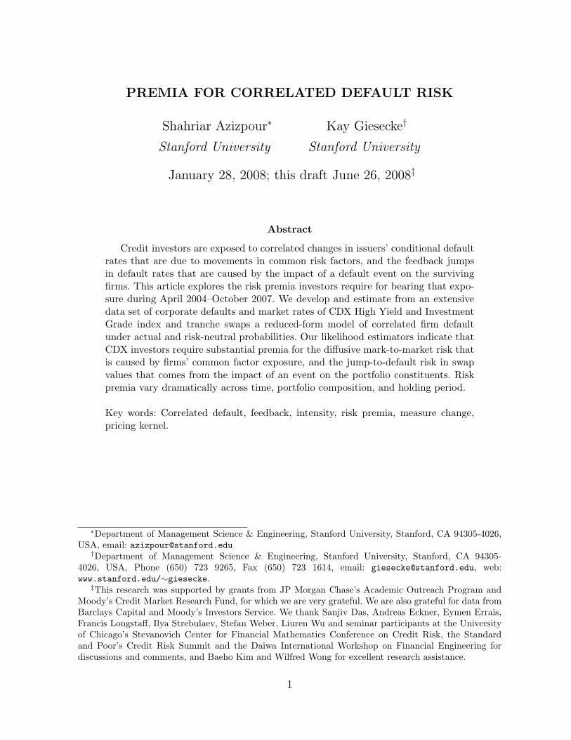
Figure 1: Left panel : Annual default data. A bar represents the number of events in a

given year. The shaded part of the bar represents the number of days over which these

events are distributed. Right panel : Events per day. A bar represents the number of days

in the sample with a given number of events. The largest number of events occurred on

June 21, 1970, when 24 railway firms defaulted.

to a diminished financial obligation; or (ii) the exchange had the apparent purpose of

helping the borrower avoid default.

We observe a total of 1398 defaults on 930 distinct dates. The distribution of these

defaults over the dates is shown in Figure 1. The data do not permit us to distinguish

the exact default timing during the day. Roughly 51% of the defaults are due to missed

interest payments and 25% are due to Chapter 11. Of the defaulted firms, 84% are of

Moodys “Industrial” category and 85% are domiciled in the United States. Defaulters are

rated in the categories IG, Ba, B, Caa, Ca, C and WR, where the WR category designates

defaulters that were not rated at the event.

A repeated default by the same issuer is included in the set of events if it was not

within a year of the initial event and the issuer’s rating was raised above Caa after the

initial default. This treatment of repeated defaults is consistent with that of Moodys.

There are a total of 46 repeated defaults in our database.

2.2 Economy-wide intensity

The strictly increasing sequence (Tn) of the 930 default dates in our database generate a

non-explosive counting process H with increments of size 1 and intensity h, relative to a

complete probability space (Ω,F , P ) and an observation filtration F = (Ft)t≥0 satisfying

the usual conditions. Mathematically, this means that the process defined by Ht−∫ t

0hsds

is a local martingale with respect to the filtration F and the measure P , the actual (data-

generating) measure. Intuitively, conditional on the information set Ft at time t, the

5

likelihood of events between times t and t+ ∆ is approximately ht∆ for small ∆.

Motivated by the statistical arguments and the results of the model specification

analysis in Azizpour & Giesecke (2008), we suppose that the economy-wide intensity h

evolves through time according to the model

dht = κ(c− ht)dt+ δdJt (1)

where κ ≥ 0, c = h0 > 0 and δ ≥ 0 are parameters and J is a jump process given by

Jt =∑n≥1

(Dn + wD2n)1Tn≤t (2)

where w ≥ 0 is a parameter and Dn is the number of defaults on the event date Tn. The

variable Dn ∈ FTn is drawn from a fixed distribution, independently of the event dates

(Tm)m≤n and the previous (Dm)m<n. At an event date, the response process J jumps and

so does the intensity. Therefore, an event temporarily increases the likelihood of further

arrivals. The parameters δ and w govern the response of the intensity to the number of

events at an event date. The more numerous the events the stronger the feedback. After

an event the intensity reverts to the level c exponentially at rate κ.

The intensity model (1)–(2) offers two potential channels for the substantial default

clustering found in the arrival data (Figure 1). Through the response term δJ , a default

has an impact on the default rates of the surviving firms. The feedback from events to

arrival rates can be interpreted in terms of contagion, which is propagated through the

complex web of contractual relationships in the economy. Jorion & Zhang (2007b) and

others provide evidence that in such a network, the default of a firm tends to weaken the

others. For example, Delphi’s collapse in 2005 jeopardized General Motor’s production

flow, and increased the likelihood of GM’s failure. The feedback from events to arrival

rates can also be interpreted in terms of informational asymmetries. As in Collin-Dufresne

et al. (2003), Delloye, Fermanian & Sbai (2006), Duffie, Eckner, Horel & Saita (2006),

Giesecke (2004) and others, firms may have a common source of frailty, a stochastic

default risk factor that is unobservable relative to the filtration F, and whose posterior

distribution is updated with information arrival. For example, the collapse of Enron may

have revealed dubious accounting practices that may have been in use at other firms, and

thus may have had an influence on the conditional default rates of these firms. For this

frailty interpretation of our model, we view the observation filtration F as a sub-filtration

of a complete information filtration that is not explicitly specified. Further, the process h

is viewed as the (optional) projection of the complete information intensity onto F.

Our intensity model can be extended to include additional sources of diffusive or

jump uncertainty that modulate the intensity between events. However, the specifica-

tion analysis in Azizpour & Giesecke (2008) indicates that the inclusion of a square-root

Brownian term does not improve the fit to the default data, even if additional explanatory

default covariates are used in the estimation. Also, other polynomial weight specifications

in the jump response process (2) were found to perform worse than the quadratic model

6

we propose to use. Therefore, we adopt the relatively parsimonious model (1)–(2). Below

we use goodness-of-fit tests to show that this simple model provides enough flexibility to

accurately capture the default clustering in the data.

2.3 Likelihood estimators

The data consist of pairs (Tn, Dn)n=1,...,Hτ of event dates and counts observed through time

τ , October 2007. The parameter vector to be estimated is of the form Θ = (κ, c, δ, w).

The law of the vector D = (D1, . . . , DHτ ) is described by the empirical distribution

of the sequence (Dn). By a measure change argument, the conditional joint “density”

fτ (Hτ , T ; Θ |D) of Hτ and the vector T = (T1, . . . , THτ ) given D satisfies

log fτ (Hτ , T ; Θ |D) = −cτ −Hτ−1∑n=1

∫ THτ

Tn

δe−κ(t−Tn)(Dn + wD2n)dt

+Hτ∑n=1

log(c+

n−1∑k=1

δe−κ(Tn−Tk)(Dk + wD2k)). (3)

To estimate the parameter vector Θ, we consider the maximum likelihood problem

supΘ

log fτ (Hτ , T ; Θ |D). (4)

The properties of the corresponding maximum likelihood estimator are developed in Ogata

(1978). The estimator is shown to be consistent, asymptotically normal, and efficient. We

solve the likelihood problem numerically by performing a grid search over the discretized

parameter space. Rather than optimizing over the full parameter space, we fix a set of

candidate values 0, 0.05, 0.1, . . . , 1 for w and optimize over the remaining parameters

(κ, c, δ) for each of these candidate values. Then the model is selected according to the

quality of the fit to the default data rather than the log-likelihood score.3

The goodness-of-fit of an intensity specification is evaluated with the time-scaling

tests developed by Das, Duffie, Kapadia & Saita (2007) for doubly-stochastic intensity

models. Azizpour & Giesecke (2008) show how these tests can be extended to arbitrary

intensity models, including the model (1) studied here. The extension is based on a result

of Meyer (1971), which implies that the counting process H can be transformed into a

standard Poisson process by a stochastic change of time that is given by the cumulative

intensity. If h is correctly specified, then the time-scaled event dates form a realization of a

standard Poisson process in the time-scaled filtration, which we test using a Kolmogorov-

Smirnov (KS) test and Prahl’s (1999) test. The KS test addresses the deviation of the

empirical distribution function of the time-scaled inter-arrival times from their theoretical

standard exponential distribution function. Prahl’s test is particularly sensitive to large

deviations of the time-scaled times from their theoretical mean 1.3This procedure is motivated by the observation that, due to the extreme cluster of 24 railway defaults

in 1970, the likelihood function is decreasing in w.

7

0 1 2 3 4 5 60

0.1

0.2

0.3

0.4

0.5

0.6

0.7

0.8

0.9

1

0 1 2 3 4 5 6 70

1

2

3

4

5

6

7

8

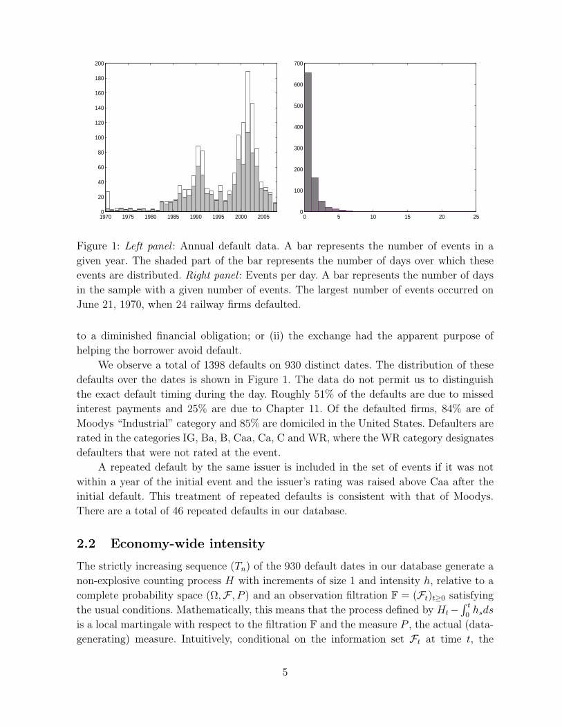
Figure 2: Empirical distribution of time-scaled inter-arrival times generated by the fitted

model. Left panel : Histogram of time-scaled inter-arrival times vs. standard exponen-

tial density function (solid line). Right panel : Empirical quantiles of time-scaled inter-

arrival times vs. theoretical standard exponential quantiles. 927 out of 930 observations

are shown: we ignore three outliers due to the cluster of railway defaults on June 21, 1970

(24 events) and June 26, 1972 (4 events).

Our estimator of Θ is given by Θ = (1.81, 5.77, 0.40, 0.50). The fitted values for δ and

w indicate the significant influence of defaults on arrival rates, and suggest the presence

of substantial feedback from events through contagion or frailty. Figure 2 contrasts the

empirical distribution of the time-scaled inter-arrival times generated by the fitted inten-

sity h with the theoretical standard exponential distribution. The KS test indicates that

the deviation of the empirical distribution of the time-scaled inter-arrival times from the

exponential distribution is not significant at the 5% level. Prahl’s test statistic is within

0.1 standard deviations from its theoretical mean, also indicating that the deviation of

the time-scaled times from their theoretical distribution is not significant.

The results of the goodness-of-fit tests indicate that the estimated model (1) of the

economy-wide intensity h replicates the substantial time-series variation of default rates in

the universe of Moodys rated firms during 1970–2007. Next we thin h to obtain estimates

of default intensities for portfolios of rated firms.

2.4 Portfolio intensity

Consider a finite portfolio of Moodys rated firms and let N be the counting process of

defaults in the portfolio. Suppose N has increments of size 1 and intensity λ, meaning

that the process Nt−∫ t

0λsds is a martingale relative to P . The intensity λt represents the

conditional portfolio default rate at t given the information set Ft. It is equal to the sum

8

of the single firm intensities λkt over the portfolio constituents k that have survived to t.4

To estimate the λk from the fitted economy-wide intensity h, consider the process Hρ that

records the number of events in rating category ρ, given by Hρt =

∑n≥1D

ρn1Tn≤t where

Dρn is the number of ρ-rated firms that default at the event date Tn. The total number

of events at Tn is Dn =∑

ρDρn. Assuming that the Dρ

n are independent across ρ and n,

the process Hρ has intensity hρ = hE[Dρn], which represents the total default intensity of

all ρ-rated firms in our database.5 The Dρn are modeled by their empirical distribution.6

Now let Xρt be the index set of ρ-rated firms in our database that have survived to time t.

Assuming that each ρ-rated firm is equally likely to default at an event date, we propose

to estimate the intensity λkt of an ρ-rated firm k ∈ Xρt by the ratio hρt /|X

ρt |. Then, with

Y ρt denoting the index set of ρ-rated firms in the portfolio that have survived to time t,

the actual portfolio default intensity λt is estimated by7

λt = ht∑ρ

|Y ρt ||Xρ

t |E[Dρn

]. (5)

We consider the CDX High Yield (HY) and Investment Grade (IG) index portfolios.

As of October 2007, the on-the-run HY index consists of 2 Baa, 48 Ba, 36 B and 14 Caa

rated firms, giving a total of 100 constituents. The on-the-run IG index consists of 3 Aaa,

3 Aa, 51 A, 64 Baa and 4 Ba rated firms (125 constituents). We account for revisions of

the portfolio compositions (“index rolls”), which take place every 6 months.8

Figure 3 graphs the fitted portfolio intensities λ from August 2004, when the indexes

were established, to October 2007. There is a clear downward trend in the conditional

default rates for both portfolios. This trend echoes the decline of overall default rates of

Moodys rated firms during that period, as indicated in Figure 1. In October 2007, these

default rates were at historically low levels. The spike in the intensity that is visible for

the IG portfolio and pronounced for the HY portfolio is triggered by defaults of three

Caa-rated industrial firms during August and the defaults of Delta Air Lines (C-rated)

and Northwest Airlines (Caa-rated) on September 14, 2005.

For the risk premium analysis in Section 4 below, we require the fitted portfolio in-

tensity λ only for the period 2004–2007. Nevertheless, to estimate λ we use the entire

Moodys default history, which covers the period 1970–2007. Since defaults are typically

low-probability events, we need to include as many observations as possible in the estima-

4Here, λk is a process such that Nkt −

∫ t0λks(1 −Nk

s )ds is a P -martingale, where Nk is the indicatorprocess associated with the default of firm k. See Giesecke & Goldberg (2005) for more details.

5More precisely, the process defined by Hρt −

∫ t0hρsds is a martingale relative to P .

6Instead of inferring hρ from h, we could have specified separate intensity models hρ for the total ofall firms in a given rating category ρ. A model hρ could have been estimated from the observed eventtimes of ρ-rated firms, which form a subset of the sequence (Tn).

7This estimate ignores the probability of observing more than just one event in the portfolio on thesame day. Based on our event data, we find that this probability is negligible.

8For the roll dates and the list of constituents that are exchanged at each roll see the websitewww.markit.com of Markit, the calculation agent for the CDX.

9

Aug04 Feb05 Aug05 Mar06 Sep06 Mar07 Oct07

0.7

0.8

0.9

1

1.1

1.2

1.3

1.4

1.5

1.6

Aug04 Feb05 Aug05 Mar06 Sep06 Mar07 Oct070.005

0.01

0.015

0.02

0.025

0.03

0.035

Figure 3: Fitted portfolio default intensity, measured in events per year. Left panel: CDX

High Yield index portfolio. Right panel: CDX Investment Grade index portfolio.

tion in order to accurately fit the arrival rate λ. If we had chosen to base the estimation of

λ on the default observations during 2004–2007 only, then the sample would have included

only 110 events instead of 1400 events.

3 Risk-neutral intensity from CDX market rates

Having estimated the intensity λ of the portfolio default process N under the actual

probability measure P , in this section we use market prices of CDX portfolio derivatives to

estimate the intensity of N under a risk-neutral pricing measure. The risk-neutral intensity

reflects the market valuation of correlated corporate default risk. We are interested in how

this market valuation differs from the actual default expectations embedded in λ.

We assume that there are no arbitrage opportunities or market frictions. Then, under

mild technical conditions, there exists a risk-neutral probability measure that is equivalent

to the actual probability measure P . We fix a risk-neutral measure P ∗ with respect to a

constant risk-free interest rate r > 0. The change of measure will be made precise as we

proceed. Technical details are in Appendix A.

3.1 Index and tranche swap pricing

We adopt the valuation approach of Errais, Giesecke & Goldberg (2006), according to

which a portfolio derivative is viewed as a contingent claim on the portfolio default process

N or the portfolio loss process L =∑N

n≥0 `n, where `n is the random loss at the nth

default. An index swap referenced on a CDX portfolio is one of the most liquid portfolio

derivatives. It is based on a portfolio whose C constituent single-name credit swaps have

common notional that we normalize to 1, common maturity date T and common quarterly

10

premium payment dates (tm). The protection seller agrees to cover portfolio losses as they

occur. The value Dt at time t ≤ T of these payments is given by the discounted cumulative

losses. By integration by parts, we get the formula

Dt = e−r(T−t)E∗t[LT]− Lt + r

∫ T

t

e−r(s−t)E∗t[Ls]ds (6)

where E∗t denotes conditional expectation under the risk-neutral measure P ∗ with respect

to the information set Ft. The protection buyer agrees to make a stream of premium

payments at dates (tm). The cash flow at tm is a fraction I of the total notional on the

names that have survived until tm. Neglecting premium accruals, the value at time t ≤ T

of the premium payments is given by

Pt(I) = I∑m

e−r(tm−t)cm(C − E∗t

[Ntm

])(7)

where cm is the appropriate day count fraction for the period m. The fair index swap

spread at time t is the solution I = It to the equation Dt = Pt(I). The spread depends

only on expected defaults and losses for horizons in (t, T ].

Investors seeking narrower risk profiles can trade tranches referenced on the CDX. A

tranche swap is specified by a lower attachment point K ∈ [0, 1] and an upper attachment

point K ∈ (K, 1]. The product of the difference K = K −K and the portfolio notional

C is the tranche notional. The tranche protection seller agrees to cover portfolio losses as

they occur, given that the cumulative losses are larger than KC but do not exceed KC.

The cumulative payments at time t, denoted Ut, are

Ut = (Lt −KC)+ − (Lt −KC)+.

The value of these payments at time t is

Dt(K,K) = e−r(T−t)E∗t[UT]− Ut + r

∫ T

t

e−r(s−t)E∗t[Us]ds. (8)

This formula is analogous to formula (6) for the value of an index swap default leg. The

latter can be viewed as the default leg of a tranche swap for which K = 0 and K = 1. The

premium payments of the tranche protection buyer consist of two parts. The first part is

an upfront payment, which is expressed as a fraction R of the tranche notional KC. The

second part is a stream of payments at dates (tm). For a tranche with K < 1, the cash

flow at tm is a fraction S of the difference between the tranche notional and the tranche

loss at tm. Neglecting accruals, the value of the premium leg is given by

Pt(K,K,R, S) = RKC + S∑m

e−r(tm−t)cm(KC − E∗t

[Utm]). (9)

For a fixed upfront payment rate R, the fair tranche spread S is the solution S =

St(K,K,R) to the equation Dt(K,K) = Pt(K,K,R, S). Similarly, for a fixed tranche

spread S, the fair tranche upfront rate R is the solution R = Rt(K,K, S) to the equation

Dt(K,K) = Pt(K,K,R, S). The fair spread and upfront rate depend only on the value

of call spreads on the portfolio loss Ls with strikes K and K and maturities s ∈ (t, T ].

11

3.2 Risk-neutral portfolio intensity

To value CDX index and tranche swaps, we model the default and loss processes under

the risk-neutral measure P ∗. The default counting process N is specified in terms of a

risk-neutral intensity λ∗ that represents the conditional portfolio default rate with respect

to P ∗. More precisely, we suppose that there is a process λ∗ such that the compensated

default counting process, given by Nt −∫ t

0λ∗sds, is a martingale relative to P ∗. The risk-

neutral intensity λ∗ is the counterpart to the actual intensity λ of N estimated in Section

2 above. As indicated in Appendix A, modeling λ∗ for a given specification of λ amounts

to identifying the Radon-Nikodym derivative that defines the change of measure from P

to P ∗, i.e., the pricing kernel of the economy.

The maximum likelihood approach to estimating λ∗ that we propose requires us

to specify the distribution of λ∗ under both P and P ∗. We suppose that under actual

probabilities, λ∗ evolves through time according to the model

dλ∗t = κ∗(c∗ − λ∗t )dt+ σ∗√λ∗tdWt + δ∗dLt (10)

where κ∗, c∗, σ∗, and δ∗ are parameters with 2κ∗c∗ ≥ (σ∗)2 that satisfy the technical

conditions stated in Appendix A, W is a standard Brownian motion relative to P , and

where L =∑N

n≥0 `n is the portfolio loss process. The random loss `n is drawn from a

P -distribution ν, independently of the information set Fτn−, where τn is the nth default

time in the portfolio.9 The intensity jumps at arrivals, together with the default and loss

processes. Note that under P , the arrivals are governed by the actual intensity λ. The

jump size is proportional to the realized loss at an event.

Next we specify the distribution of λ∗ under the risk-neutral measure P ∗, which is

relevant for the valuation of index and tranche swaps. Motivated by the successful CDX

index and tranche market calibrations reported in Giesecke & Kim (2007), we suppose

that under risk-neutral probabilities, λ∗ follows the model

dλ∗t = κ∗(c∗ − λ∗t )dt+ σ∗√λ∗tdW

∗t + δ∗dLt (11)

where κ∗ = κ∗ + ησ∗, κ∗c∗ = κ∗c∗ for a parameter η such that W ∗t = Wt + η

∫ t0

√λ∗sds

is a standard Brownian motion with respect to P ∗; see Appendix A. The parameter η

represents the risk premium for the diffusive volatility of risk-neutral arrival rates. The

intensity jumps at arrivals along with N and L. The arrivals are governed by λ∗ itself. The

jump size is proportional to the realized loss at an event, `n, which we suppose is drawn

P ∗-independently of Fτn− from the distribution ν, which also governs `n under P .10

The dynamics of the risk-neutral intensity λ∗ have similar features under the two

measures. Thanks to the feedback term δ∗L, the intensity always responds to defaults.

9The parameter δ∗ can be subsumed into the distribution ν. We introduce it here to facilitate acomparison of the sensitivity of λ∗ across different portfolios that share the same ν.

10In other words, we assume that there is no premium for recovery risk. This assumption is motivatedby the fact that we observe no events for the IG portfolio and only 4 events in the HY portfolio duringthe sample period, making it difficult to accurately estimate such a premium.

12

However, the frequency of defaults differs under the two measures, and so does the fre-

quency of the jumps in λ∗: they arrive at rate λ under P and rate λ∗ under P ∗. The size

of the response jumps is inversely proportional to the realized recovery at an event. The

lower the recovery, the larger the increase of the intensity at the event. This specification

replicates the negative correlation between recovery and default rates found by Altman,

Brady, Resti & Sironi (2005) and others. After an event, the intensity reverts back to a

constant level, which is given by c∗ under P , and c∗ under P ∗. The decay is exponential

in mean, with rate κ∗ under P and rate κ∗ under P ∗. These four parameters are related

through the constraint κ∗c∗ = κ∗c∗, which is imposed by our “completely affine” specifi-

cation of the market price of risk for W .11 The diffusive fluctuations of λ∗ between events

are governed by the square-root Brownian term, whose volatility is σ∗.

Our model specification allows us to derive computationally tractable expressions for

index and tranche swap rates. Since the processes N and L are affine point processes in

the sense of Errais et al. (2006), the characteristic function of (N,L)> is an exponentially

affine function of the state. We have the formula

E∗t[

exp(iv(LT − Lt)

)]= exp

(α(t) + β(t)λ∗t

)(12)

where t ≤ T , i is the imaginary unit, v is a real number and the coefficient functions

α(t) = α(v, t, T ) and β(t) = β(v, t, T ) solve the ordinary differential equations

∂tβ(t) = 1 + κ∗β(t)− 1

2(σ∗)2β(t)2 − q(δ∗β(t), v) (13)

∂tα(t) = −c∗κ∗β(t) (14)

with boundary conditions β(T ) = α(T ) = 0 and jump transform

q(u, v) =

∫e(iv+u)zdν(z)

where ν is the distribution of the loss at default `n, and u is any complex number such

that q(u, v) is well defined for a given real v. The characteristic function of N is given by

the right hand side of equation (12), with coefficient functions α(t) and β(t) satisfying

equations (13)–(14), where q(u, v) is replaced by qN(u, v) =∫eiv+uzdν(z).

Conditional expected defaults E∗t [NT ] and losses E∗t [LT ] are obtained by differenti-

ating the corresponding characteristic functions. We obtain closed form expressions for

these expectations. From equations (6) and (7), we then get a closed form expression for

the model index swap spread It. Model tranche rates do not take a closed form. We first

obtain the conditional loss distribution by Fourier inversion of the characteristic function

(12). The price of an option on L is gotten by integrating the option payoff against the loss

distribution. The option price determines the tranche rate through formulae (8)–(9).12

11We do not opt for the more comprehensive “extended affine” risk premium specification proposed byCheridito, Filipovic & Kimmel (2007), largely because our sample period is relatively short.

12Alternatively, tranche rates can be estimated by Monte Carlo simulation of L. Giesecke & Kim (2007)provide an exact simulation algorithm for the model (11).

13

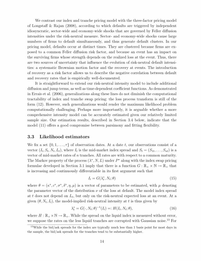
We contrast our index and tranche pricing model with the three-factor pricing model

of Longstaff & Rajan (2008), according to which defaults are triggered by independent

idiosyncratic, sector-wide and economy-wide shocks that are governed by Feller diffusion

intensities under the risk-neutral measure. Sector- and economy-wide shocks cause large

numbers of firms to default simultaneously, and thus generate default clusters. In our

pricing model, defaults occur at distinct times. They are clustered because firms are ex-

posed to a common Feller diffusion risk factor, and because an event has an impact on

the surviving firms whose strength depends on the realized loss at the event. Thus, there

are two sources of uncertainty that influence the evolution of risk-neutral default intensi-

ties: a systematic Brownian motion factor and the recovery at events. The introduction

of recovery as a risk factor allows us to describe the negative correlation between default

and recovery rates that is empirically well-documented.

It is straightforward to extend our risk-neutral intensity model to include additional

diffusion and jump terms, as well as time-dependent coefficient functions. As demonstrated

in Errais et al. (2006), generalizations along these lines do not diminish the computational

tractability of index and tranche swap pricing: the loss process transform is still of the

form (12). However, such generalizations would render the maximum likelihood problem

computationally challenging. Perhaps more importantly, it is arguable whether a more

comprehensive intensity model can be accurately estimated given our relatively limited

sample size. Our estimation results, described in Section 3.4 below, indicate that the

model (11) offers a good compromise between parsimony and fitting flexibility.

3.3 Likelihood estimators

We fix a set 0, 1, . . . , τ of observation dates. At a date t, our observations consist of a

vector (It, St, Nt, Lt), where It is the mid-market index spread and St = (S1t, . . . , Snt) is a

vector of mid-market rates of n tranches. All rates are with respect to a common maturity.

The Markov property of the process (λ∗, N, L) under P ∗ along with the index swap pricing

formulae developed in Section 3.1 imply that there is a function G : R+ × N → R+ that

is increasing and continuously differentiable in its first argument such that

It = G(λ∗t , Nt; θ) (15)

where θ = (κ∗, c∗, σ∗, δ∗, η, µ) is a vector of parameters to be estimated, with µ denoting

the parameter vector of the distribution ν of the loss at default. The model index spread

at t does not depend on Lt, but only on the risk-neutral expected loss at an event. At a

given (θ,Nt, It), the model-implied risk-neutral intensity at t is thus given by

λ∗t = G(·, Nt; θ)−1(It) =: H(It, Nt; θ), (16)

where H : R+×N→ R+. While the spread on the liquid index is measured without error,

we suppose the rates on the less liquid tranches are corrupted with Gaussian noise.13 For

13While the bid/ask spreads for the index are typically much less than 1 basis point for most days inthe sample, the bid/ask spreads for the tranches tend to be substantially higher.

14

functions Fk : R+ × R+ → R+ implied by the pricing formulae developed in Section 3.1,

Skt = Fk(λ∗t , Lt; θ) exp(εkt), k = 1, . . . , n (17)

where εkt is a normally distributed random variable with mean zero and variance v2k, with

respect to the actual probability measure P . The error variables εkt are independent of

one another, and independent across tranches and observation dates, under P . We let

v = (v1, . . . , vn) denote the standard deviation of the errors. Note that the model tranche

rate Skt does not depend on the default count Nt.

The index spread is the transformed value of the latent risk-neutral intensity, with the

index pricing function (15) defining the transformation. By standard change of variable

arguments we obtain the log-likelihood function of the data as

L(θ, v) =τ∑t=1

log gt(H(It, Nt; θ); θ |H(It−1, Nt−1; θ), Nt−1, Lt−1, Nt, Lt

)+ log g0

(H(I0, N0; θ); θ |N0, L0

)+

τ∑t=1

log |∂1H(It, Nt; θ)|+ LN,L

+τ∑t=1

n∑k=1

[log φ

(logSkt − logFk(H(It, Nt; θ), Lt; θ); v

2k

)− logSkt

]where gt(·; θ |λ∗t−1, Nt−1, Lt−1, Nt, Lt) is the conditional density of λ∗t and g0(·; θ |N0, L0)

is the conditional density of λ∗0, both under P . Note from equation (10) that λ∗ follows a

P -Feller diffusion between events. The jumps in λ∗ arrive with P -intensity λ. Therefore,

if Nt−1 = Nt then gt(·; θ |λ∗t−1, Nt−1, Lt−1, Nt, Lt) is the non-central chi-squared density,

which is easily calculated.14 The function ∂1H(·, ·; θ) is the partial derivative of H(·, ·; θ)with respect to its first argument. It enters into the third term of the log-likelihood

function, which reflects the fact that the risk-neutral intensity is extracted from the index

spread observation. The fourth term LN,L represents the log-likelihood function of the

vector (N0, L0, . . . , Nτ , Lτ ). This likelihood is determined by the P -intensity model λ,

which was already estimated in Section 2 above, and the P -distribution ν of the loss at

events, which is specified by the parameter vector µ. Finally, the last term of the log-

likelihood function accounts for the noisy tranche rate observations, where φ(·;V ) is the

density of a Gaussian random variable with mean zero and variance V .

The likelihood problem has features that are unique to the multi-name setting. While

a credit swap referenced on an individual issuer expires at default, index and tranche swap

rates are quoted until maturity, even after the reference portfolio suffers defaults. Model

index and tranche rates depend on the number of events and the cumulative loss induced

14There were no events in the IG portfolio during the sample period. There were 4 events in the HYportfolio. Of these, one falls on a Wednesday, two fall on a Tuesday and one falls on a Saturday. Forthe purpose of calculating the conditional density, we move the latter three events to the immediatelyfollowing Wednesday, the weekday on which we observe the price data.

15

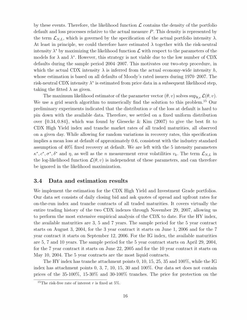
by these events. Therefore, the likelihood function L contains the density of the portfolio

default and loss processes relative to the actual measure P . This density is represented by

the term LN,L, which is governed by the specification of the actual portfolio intensity λ.

At least in principle, we could therefore have estimated λ together with the risk-neutral

intensity λ∗ by maximizing the likelihood function L with respect to the parameters of the

models for λ and λ∗. However, this strategy is not viable due to the low number of CDX

defaults during the sample period 2004–2007. This motivates our two-step procedure, in

which the actual CDX intensity λ is inferred from the actual economy-wide intensity h,

whose estimation is based on all defaults of Moody’s rated issuers during 1970–2007. The

risk-neutral CDX intensity λ∗ is estimated from price data in a subsequent likelihood step,

taking the fitted λ as given.

The maximum likelihood estimator of the parameter vector (θ, v) solves supθ,v L(θ, v).

We use a grid search algorithm to numerically find the solution to this problem.15 Our

preliminary experiments indicated that the distribution ν of the loss at default is hard to

pin down with the available data. Therefore, we settled on a fixed uniform distribution

over 0.34, 0.84, which was found by Giesecke & Kim (2007) to give the best fit to

CDX High Yield index and tranche market rates of all traded maturities, all observed

on a given day. While allowing for random variations in recovery rates, this specification

implies a mean loss at default of approximately 0.6, consistent with the industry standard

assumption of 40% fixed recovery at default. We are left with the 5 intensity parameters

κ∗, c∗, σ∗, δ∗ and η, as well as the n measurement error volatilities vk. The term LN,L in

the log-likelihood function L(θ, v) is independent of these parameters, and can therefore

be ignored in the likelihood maximization.

3.4 Data and estimation results

We implement the estimation for the CDX High Yield and Investment Grade portfolios.

Our data set consists of daily closing bid and ask quotes of spread and upfront rates for

on-the-run index and tranche contracts of all traded maturities. It covers virtually the

entire trading history of the two CDX indexes through November 29, 2007, allowing us

to perform the most extensive empirical analysis of the CDX to date. For the HY index,

the available maturities are 3, 5 and 7 years. The sample period for the 5 year contract

starts on August 3, 2004, for the 3 year contract it starts on June 1, 2006 and for the 7

year contract it starts on September 12, 2006. For the IG index, the available maturities

are 5, 7 and 10 years. The sample period for the 5 year contract starts on April 29, 2004,

for the 7 year contract it starts on June 22, 2005 and for the 10 year contract it starts on

May 10, 2004. The 5 year contracts are the most liquid contracts.

The HY index has tranche attachment points 0, 10, 15, 25, 35 and 100%, while the IG

index has attachment points 0, 3, 7, 10, 15, 30 and 100%. Our data set does not contain

prices of the 35-100%, 15-30% and 30-100% tranches. The price for protection on the

15The risk-free rate of interest r is fixed at 5%.

16

Index Maturity Start κ∗ c∗ σ∗ δ∗ η v1 v2 v3 v4

3Y 06/01/06 1.30 1.20 1.70 1.00 0.50 0.07 0.30 0.50 0.80

HY 5Y 08/03/04 1.80 1.50 1.90 1.30 0.70 0.05 0.14 0.18 0.42

7Y 09/12/06 1.60 1.30 1.90 1.30 0.50 0.04 0.08 0.06 0.30

5Y 04/29/04 0.35 0.85 0.75 0.20 0.30 0.07 0.55 0.38 1.05

IG 7Y 06/22/05 1.10 0.40 0.90 0.70 1.00 0.06 0.46 0.68 0.14

10Y 05/10/04 0.50 0.30 0.50 0.50 0.70 0.07 0.15 0.60 0.60

Table 1: Maximum likelihood estimates of the risk-neutral intensity parameters and the

tranche measurement error volatilities vk. The “Start” column indicates the beginning of

the observation period. The observation period ends on November 29, 2007.

0–10% and 10–15% HY tranches is quoted in terms of an upfront rate, while the price for

protection on the 0–3% IG tranche is quoted in terms of an upfront rate plus a spread of

500 basis points that is paid quarterly. All other tranches are quoted in terms of a running

spread that is paid quarterly. To reduce the noise in the data, we use weekly mid-market

quotes, usually observed on Wednesdays. If a Wednesday quote is not available, we use

the average of the Tuesday and Thursday quotes. This leaves us with 158 quotes for the 5

year IG contracts and 156 quotes for the 5 year HY contracts. To facilitate the estimation

of the diffusive risk premium η, we ignore index rolls.16

In view of the different observation periods, we perform the estimation separately

for each available contract maturity. The corresponding maximum likelihood parameter

estimates are given in Table 1. The feedback coefficients δ∗ are estimated to be strictly

positive, indicating that a default has a substantial impact on CDX index and tranche

market rates. The impact is stronger for the HY contracts, which are referenced on low-

quality firms. The fitted decay rates κ∗ suggest that the impact is more persistent for

the IG contracts. The HY portfolio is estimated to have a greater base default rate, as

indicated by the fitted reversion levels c∗. Also the diffusive volatility σ∗ of default rates

is estimated to be higher for the HY portfolio. The fitted values of the market price of

risk η for W are discussed in Section 4.

Figure 4 shows the time series of the fitted risk-neutral default intensities for the

HY and IG portfolios, based on the estimates for the 5 year contracts. Given a pair

of observations (It, Nt), the fitted risk-neutral intensity at t is obtained from formula

(16) evaluated at the maximum likelihood estimator θ. There were no defaults in the

IG portfolio so Nt = 0 for all observation dates t. The HY portfolio experienced four

defaults during the sample period: Collins & Aikman Products Co. 05/17/05, Delphi

Corp. 10/8/05, Calpine Corp. 12/20/05 and Dana Corp. 03/01/06.

16We can account for index rolls by estimating separate risk-neutral intensity models for each of the 6month roll periods. It will however be extremely difficult to pin down η, the market price of risk for W ,for a sample period that is only 6 months long.

17

Aug04 Feb05 Sep05 Mar06 Oct06 May07 Nov072

4

6

8

10

12

14

16

Aug04 Feb05 Sep05 Mar06 Oct06 May07 Nov070

0.2

0.4

0.6

0.8

1

1.2

1.4

Figure 4: Fitted risk-neutral portfolio default intensity, measured in events per year, based

on 5 year maturity index and tranche swaps. Left panel: CDX High Yield index portfolio.

Right panel: CDX Investment Grade index portfolio.

As expected, the HY intensity is higher than the IG intensity. The intensities spiked

during May 2005, with the IG intensity experiencing a relatively larger increase than the

HY intensity. These spikes reflected the broad widening of spreads due to anticipated

problems in the auto industry, triggered by the downgrades of Ford and GM. After a

relatively quiet period, the intensities again sharply increased more recently during the

spring and summer of 2007 in response to the signs of a credit crisis in the U.S. The

increase in the IG intensity was proportionately bigger than that in the HY intensity.

3.5 Tranche pricing errors

Our estimation assumes that index spreads are measured without error. Therefore, they

are always matched perfectly. Tranche rates are corrupted with noise so they are not fitted

exactly. We compare market tranche rates with model-implied rates Fk(λ∗t , Lt; θ), where

λ∗t is the fitted risk-neutral intensity obtained from formula (16), and θ is the maximum

likelihood estimator of θ. For the purpose of calculating the model-implied rates, we

assume a realized recovery rate of 40% for the four HY defaults during the sample period,

consistent with standard industry practice and the mean loss at default we assume in the

estimation. Figure 5 shows the time series of observed and fitted 5 year HY tranche rates.

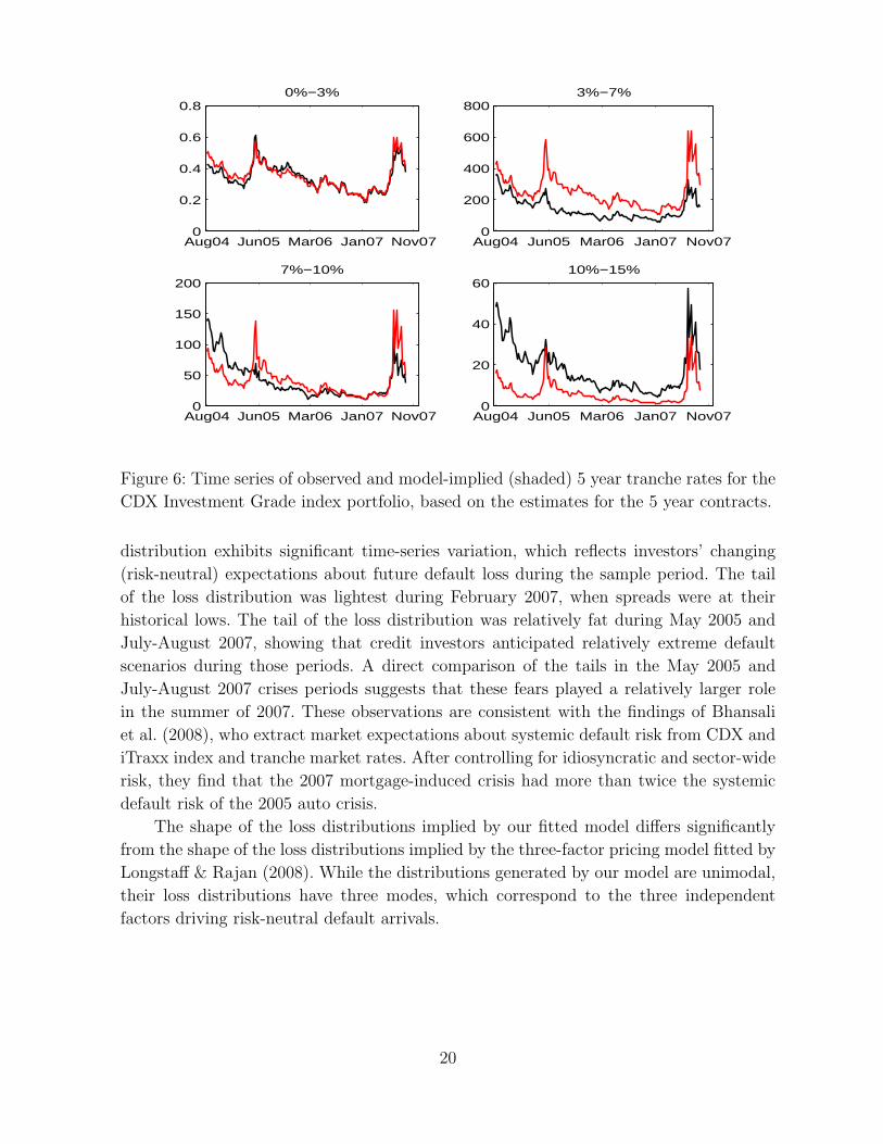
Figure 6 graphs the time series for the 5 year IG tranches.

The model replicates the substantial cross-sectional and extreme time-series variation

of CDX tranche rates during 2004–2007. While the tranche pricing errors vary consider-

ably, they do not seem to follow a particular pattern. As a diagnostic check, we examine

18

Aug04 Jun05 Apr06 Feb07 Nov07

0.7

0.8

0.9

10%−10%

Aug04 Jun05 Apr06 Feb07 Nov070.2

0.4

0.6

0.8

110%−15%

Aug04 Jun05 Apr06 Feb07 Nov070

500

1000

150015%−25%

Aug04 Jun05 Apr06 Feb07 Nov070

100

200

300

40025%−35%

Figure 5: Time series of observed and model-implied (shaded) 5 year tranche rates for the

CDX High Yield index portfolio, based on the estimates for the 5 year contracts.

the empirical distribution of the logarithm of the relative tranche pricing errors

εkt = log

(Skt

Fk(λ∗t , Lt; θ)

), k = 1, . . . , n, (18)

where Skt is the market rate of the kth tranche at t. Under the specified model, and

under actual probabilities, these errors are independent across tranches k and observation

dates t, and are normally distributed with mean zero and variance v2k. Figure 7 shows the

histogram of the standardized errors across all 5 year tranches. The empirical distribution

of the HY errors is in good agreement with the standard normal distribution, indicating

the adequacy of our model specification for the HY portfolio. The empirical distribution

of the IG errors indicates that the model fits the IG tranche rates less well. However,

since the deviations from the normal distribution are largely symmetric, the model does

not exhibit a significant pricing bias. IG tranches are only slightly overpriced: the sample

mean is −0.038 and the sample standard deviation is 1.085. For the HY tranches, the

sample mean is −0.213 and the sample standard deviation is 1.001.

3.6 Portfolio loss distribution

Figure 8 shows the risk-neutral distribution of future HY index portfolio loss for a 5

year horizon, estimated at each observation date based on the 5 year contracts. The

19

Aug04 Jun05 Mar06 Jan07 Nov070

0.2

0.4

0.6

0.80%−3%

Aug04 Jun05 Mar06 Jan07 Nov070

200

400

600

8003%−7%

Aug04 Jun05 Mar06 Jan07 Nov070

50

100

150

2007%−10%

Aug04 Jun05 Mar06 Jan07 Nov070

20

40

6010%−15%

Figure 6: Time series of observed and model-implied (shaded) 5 year tranche rates for the

CDX Investment Grade index portfolio, based on the estimates for the 5 year contracts.

distribution exhibits significant time-series variation, which reflects investors’ changing

(risk-neutral) expectations about future default loss during the sample period. The tail

of the loss distribution was lightest during February 2007, when spreads were at their

historical lows. The tail of the loss distribution was relatively fat during May 2005 and

July-August 2007, showing that credit investors anticipated relatively extreme default

scenarios during those periods. A direct comparison of the tails in the May 2005 and

July-August 2007 crises periods suggests that these fears played a relatively larger role

in the summer of 2007. These observations are consistent with the findings of Bhansali

et al. (2008), who extract market expectations about systemic default risk from CDX and

iTraxx index and tranche market rates. After controlling for idiosyncratic and sector-wide

risk, they find that the 2007 mortgage-induced crisis had more than twice the systemic

default risk of the 2005 auto crisis.

The shape of the loss distributions implied by our fitted model differs significantly

from the shape of the loss distributions implied by the three-factor pricing model fitted by

Longstaff & Rajan (2008). While the distributions generated by our model are unimodal,

their loss distributions have three modes, which correspond to the three independent

factors driving risk-neutral default arrivals.

20

−3 −2 −1 0 1 2 30

0.05

0.1

0.15

0.2

0.25

0.3

0.35

0.4

−3 −2 −1 0 1 2 30

0.05

0.1

0.15

0.2

0.25

0.3

0.35

0.4

Figure 7: Histogram of standardized relative tranche pricing errors (18) across all 5 year

tranches, and standard normal density. Left panel: CDX High Yield index portfolio. The

sample mean is −0.213 and the sample standard deviation is 1.001. Right panel: CDX

Investment Grade index portfolio. The sample mean is −0.038 and the sample standard

deviation is 1.085.

3.7 Discussion

It is instructive to contrast our statistical methodology with that employed by Longstaff

& Rajan (2008, LR) to fit an index and tranche pricing model to a time series of 5 year

CDX IG market rates. Assuming that all market rates are measured without error, LR

use a non-linear least squares algorithm to fit distinct risk-neutral three-factor models

for each of the 6 month roll periods during October 2003 to October 2005. For each of

those periods, the algorithm matches index spreads perfectly and minimizes the root mean

squared tranche pricing errors during the period.

Our maximum likelihood approach allows us to take account of measurement errors in

the tranche data. Only the spreads of the much more liquid index contracts are assumed to

be measured precisely, and these values are matched perfectly. The estimation procedure

does not directly optimize over tranche pricing errors. Therefore, the absolute root mean

squared pricing error is not the appropriate metric to assess model fit. Rather, we examine

how well the empirical distribution of fitted tranche pricing errors conforms to the specified

distribution of the errors.

The likelihood approach also allows us to estimate the dynamics of the risk-neutral

intensity under both actual and risk-neutral measures. As a result, we obtain an estimate

of the market price of risk for the Brownian motion driving the risk-neutral intensity.

This premium indicates investors’ aversion towards diffusive spread fluctuations. This

has a price, however: the premium is notoriously hard to pin down, and the associated

estimation errors may affect the quality of the fit to the tranches.

21

010

2030

40 Aug04Feb05

Sep05Mar06

Oct06May07

Nov07

0

0.02

0.04

0.06

0.08

Figure 8: Smoothed risk-neutral distribution of future loss in the CDX High Yield index

portfolio for a 5 year horizon, estimated at each observation date in the sample period

based on the 5 year contracts.

Rather than breaking up the sample period into 6 month long index roll periods and

estimating separate models for these sub-periods, we estimate one model (one set θ of

parameters) for the entire sample period. This 3.5 year period consists of very benign times

with extremely low spreads (beginning of 2007) and very turbulent ones with dramatic

spread changes and very high spread levels (summer 2007). Fitting this substantial spread

variation is much more challenging than fitting the relatively small changes in spreads that

occurred during any of the 6 month roll periods preceding 2006. Our model does a really

good job at fitting this variation, especially for the HY index.

The likelihood perspective proposed here facilitates a more holistic approach to model

fitting than the calibration approach that is typically taken in the portfolio derivatives

literature, for example Arnsdorf & Halperin (2007), Brigo et al. (2006), Cont & Minca

(2008), Ding et al. (2006) and Lopatin & Misirpashaev (2007). Using an objective function

that penalizes index and tranche pricing errors, Giesecke & Kim (2007) fit the risk-neutral

intensity model (11) to market rates of contracts of all available maturities, all observed

on the same day. While this approach is well suited to exploit term structure data, it

typically ignores time series data. Instead, the model is re-calibrated every day.

22

4 CDX risk premia

An index or tranche investor is exposed to the diffusive volatility in swap market rates

that we call non-default mark-to-market risk, and the jumps in market rates at events,

called jump-to-default risk. This section analyzes the premia that investors demand for

bearing exposure to these risks. These premia identify the equivalent change of probability

measure from actual to risk-neutral probabilities, as detailed in Appendix A.

Non-default mark-to-market risk is induced by firms’ sensitivity to a common risk

factor, which in our model is represented by the Brownian motion W . The fluctuations

of W generate correlated changes in firms’ default probabilities. The compensation for

bearing the exposure to co-movements in firms’ default probabilities is measured by the

parameter η, which identifies the change of measure for W . The fitted values for η, shown

in Table 1 above, are strictly positive for all contracts, indicating that non-default mark-

to-market risk is economically important, and priced into the CDX market.

The premium for non-default mark-to-market risk is realized as a change to the drift

of risk-neutral intensities λ∗. A positive η implies that the impact of an event on λ∗

is less persistent under P ∗. The premium for bearing correlated jump-to-default risk is

realized as a change to the intensity itself: the risk-neutral intensity λ∗ and the actual

intensity λ follow distinct processes. This change to the intensity also has implications for

the feedback jumps of λ∗ that occur at events. Under P , the jumps arrive with intensity

λ. Under P ∗, the jumps arrive with intensity λ∗. This adjustment of arrival rates can

be viewed as compensation for the abrupt changes in index and tranche mark-to-market

values at events, which are due to the impact of an event on the default rates of the

surviving single-name constituents. Constituent spreads are revised at events, and so are

index and tranche mark-to-market values. If these feedback phenomena are ignored, then

the risk-neutral intensity does not jump at events, and any compensation for jumps at

events is absorbed into the premium for non-default mark-to-market risk.

The total compensation π for any time-variation (diffusive or jump at defaults) in in-

dex and tranche market rates is measured by the difference between the jump-compensated

drift of λ∗ under P and its counterpart under P ∗. It is given by

πt = ησ∗λ∗t + δ∗E[`n](λt − λ∗t ). (19)

The first term in formula (19) represents compensation for diffusive volatility, and the

second term represents compensation for volatility due to jumps at events. The compen-

sation for jump volatility is proportional to the expected feedback jump of the risk-neutral

intensity at an event. It vanishes when event feedback is absent (δ∗ = 0). Figure 9, which

displays the fitted π for 5 year contracts, indicates that CDX IG investors require much

less compensation for the time-variation in index and tranche rates than HY investors.

The compensation for variation in IG rates was almost zero at the end of February 2007,

when spreads were at their historical lows. It spiked during the auto crisis in May 2005

and the mortgage crisis in the summer of 2007.

23

Aug04 Feb05 Aug05 Mar06 Sep06 Mar07 Oct071

2

3

4

5

6

7

8

9

10

Aug04 Feb05 Aug05 Mar06 Sep06 Mar07 Oct070

0.02

0.04

0.06

0.08

0.1

0.12

0.14

0.16

Figure 9: Fitted premia π for any time-variation (diffusive or jump at events) in 5 year

index and tranche mark-to-market values. Left panel: CDX High Yield index portfolio.

Right panel: CDX Investment Grade index portfolio.

The case λ∗ = λ would imply that index and tranche investors are not requiring

compensation for correlated jump-to-default risk. In that case, CDX risk premia would

be entirely due to non-default mark-to-market risk, and the change of measure from P

to P ∗ would be completely specified by η. Jarrow et al. (2005) provide conditions under

which actual and risk-neutral single-firm intensities agree. A sufficient condition is that

there are infinitely many firms, all exposed to the same risk factor, and all defaulting

independently conditional on the risk factor. In our model specification, the conditional

independence (doubly-stochastic) assumption is violated because a default event has an

impact on the surviving firms. Therefore, a default event may command a premium even

if the portfolio consists of a large number of firms.

We measure the jump-to-default premium by the ratio of risk-neutral portfolio in-

tensity λ∗ to actual intensity λ. This ratio specifies the change of measure for the default

process N . The risk-neutral intensity represents the market price for protection against

instantaneous defaults in the portfolio, given current market information and past defaults

and their recoveries. The actual intensity represents the expected number of instantaneous

arrivals in the portfolio, given historical default experience. The portfolio intensities in-

corporate the substantial effects of default correlation among portfolio constituents. Their

ratio can be viewed as the proportional premium for bearing correlated default event risk.

For example, if this ratio is 2 for a particular date, then an insurance contract that pays

one dollar in the event of an event in the next instant would be priced at twice the actual

instantaneous default probability.

Figure 10 graphs the fitted ratios of λ∗ to λ for the HY and IG portfolios, based

on estimates obtained from 5 year contracts. Figure 11 plots the ratios based on esti-

mates obtained from 3, 7 and 10 year contracts. The wide gaps between λ∗ and λ indicate

24

Aug04 Feb05 Sep05 Mar06 Oct06 May07 Nov072

4

6

8

10

12

14

16

18

20

Aug04 Feb05 Sep05 Mar06 Oct06 May07 Nov070

50

100

150

Figure 10: Fitted premia for correlated jump-to-default risk: ratio of risk-neutral portfolio

intensity λ∗ to actual portfolio intensity λ for 5 year contracts. Left panel: CDX High

Yield index portfolio. Right panel: CDX Investment Grade index portfolio.

that credit investors demand substantial compensation for bearing exposure to correlated

jump-to-default risk, with generally much higher jump-to-default premia for the IG port-

folio of high-quality firms, for all maturities. Note that the relation between IG and HY

contracts is reversed if we consider the total premium π for any time-variation in CDX

rates: IG investors require less compensation for time-variation than HY investors.

Jump-to-default premia vary dramatically over time. After an initial downward trend,

during the second quarter of 2005 premia increased quickly to peak in May 2005, marking

the height of the correlation crisis that is often linked to the downgrades of Ford and

General Motors. The premia spiked again in September 2006, and then steadily declined

to bottom out in late February 2007. From this trough, premia surged rapidly to peak at

historically extreme levels in early August 2007, reflecting the appearing signs of a credit

crunch in the U.S. due to strings of mortgage defaults. The premia declined somewhat

from these levels but remained relatively high through October 2007.

Figure 12 graphs the rolling relative monthly changes of the jump-to-default premia.

IG premia are much more volatile than HY premia. The largest relative changes occurred

in late February and early March 2007, during a period of heavy losses in equity markets.

IG premia climbed from a historical low of 1.65 on February 21st to 24.34 on March

7th. During that same two week period, HY premia climbed from 2.47 to 5.96. The

largest absolute changes occurred later during the summer 2007. HY premia reached

their historical high of 19.75 on August 1st, while IG premia stood at 140 on that date.

IG premia peaked at 144.11 two weeks later. While the IG jump-to-default premia are

large, the overall compensation π for any time-variation in CDX IG spreads is moderate.

The substantial changes in jump-to-default premia during July and August 2007

may be related to the unprecedented losses during the second week of August at hedge

25

Jun06 Aug06 Oct06 Dec06 Feb07 Apr07 Jun07 Aug070

2

4

6

8

10

12

14

16

18

207 Year3 Year

Jun05 Oct05 Feb06 Jun06 Oct06 Mar07 Aug0750

100

150

200

250

300

350

400

4507 Year10 Year

Figure 11: Fitted premia for correlated jump-to-default risk: ratio of risk-neutral portfolio

intensity λ∗ to actual portfolio intensity λ for 3/7 and 7/10 year contracts. Left panel:

CDX High Yield index portfolio. Right panel: CDX Investment Grade index portfolio.

funds and proprietary trading desks employing primarily “statistical arbitrage” strategies.

Khandani & Lo (2007) argue that the losses were initiated by the rapid unwinding of one or

more large quantitative equity market-neutral portfolios, “perhaps in response to margin

calls from a deteriorating credit portfolio” (page 2). Our estimates indicate that credit

concerns may indeed have played a role in the “quant crisis.” As shown in Figure 13, risk

premia increased significantly during July, with relatively larger growth in the second half

of the month. HY premia roughly doubled from 10 to 20 during July, while IG premia

increased from 40 to roughly 140. Jump-to-default premia peaked on August 1st, just 4

trading days before the quant crisis ensued.

The fitted time series behavior of jump-to-default premia echoes a common view held

by market participants that the risk of contagion from the mortgage market was perceived

highest during July and August 2007. During these months, signs of a serious mortgage

crisis appeared, and investors with exposure to corporate credit risk sought cover in the

CDX market at any price, driving index and tranche rates to unprecedented levels. Actual

corporate defaults remained at historically low levels, however.

Our interpretation is consistent with the findings of Bhansali et al. (2008), who

extract market expectations about systemic risk from the North American CDX market

and the European iTraxx market. Systemic risk represents scenarios with large numbers

of defaults. After controlling for idiosyncratic and sector-wide risk, Bhansali et al. (2008)

find that the level of systemic risk priced into the index and tranche market has been

on the rise ever since the mortgage crisis appeared in the summer of 2007. Our fitted

jump-to-default premia reflect that high level of systemic risk.

It remains to clarify the role of liquidity for the large jump-to-default premia we

estimated during the summer of 2007. While during that period default protection buyers

26

Aug04 Feb05 Sep05 Mar06 Oct06 May07 Nov07−2

0

2

4

6

8

10

12

14HYIG

Figure 12: Rolling relative monthly changes (in percent) of the ratio of risk-neutral port-

folio intensity λ∗ to actual portfolio intensity λ for the High Yield and Investment Grade

index portfolios. The estimates are based on the 5 year contracts.

clearly preferred the CDX index market to the largely illiquid single-name market, the

number and size of typical CDX trades declined and bid/ask spreads widened, especially

for the more senior tranches. However, our analysis of the time series of bid/ask spreads

showed that at their peak in August 2007, bid/ask spreads were not significantly wider

than those measured during the auto crisis in May 2005, when jump-to-default premia

stood at roughly one half of their value at the August 2007 peak. This indicates that liq-

uidity problems are unlikely to have overly inflated the jump-to-default premia estimates

for the summer of 2007.

5 Conclusion

This article develops a reduced-form model of correlated firm default under actual and

risk-neutral probabilities. Defaults are clustered because firms are exposed to a common

square-root diffusion risk factor, and because an event has an impact on the surviving

firms that is channeled through the complex web of legal, business and informational

relationships in the economy. This model is used to estimate the price for bearing exposure

to clustered corporate default risk during 2004–2007. The analysis is based on corporate

default history and market rates of index and tranche swaps referenced on the CDX High

Yield and Investment Grade portfolios of North American issuers.

We find that CDX investors require substantial, strongly time-varying premia for

the diffusive mark-to-market risk that is due to firms’ common factor exposure, and

the jump-to-default risk in swap mark-to-market values that is due to the impact of

27

04 Jul 18 Jul 01 Aug 15 Aug 29 Aug 12 Sep10

15

20

HY

04 Jul 18 Jul 01 Aug 15 Aug 29 Aug 12 Sep30

60

90

120

150

IG

HY

IG

Figure 13: Fitted premia for correlated jump-to-default risk: ratio of risk-neutral portfo-

lio intensity λ∗ to actual portfolio intensity λ for the High Yield (left scale, solid) and

Investment Grade (right scale, dashed) index portfolios for a selected set of dates. The

estimates are based on the 5 year contracts.

events on the portfolio constituents. Jump-to-default premia are higher for the Investment

Grade portfolio of high-quality firms, while the total compensation for diffusive and jump

volatility in swap values is higher for the High Yield portfolio of low-quality issuers. These

findings indicate that a significant portion of corporate default risk is not diversifiable.

This has implications for the risk management in financial institutions.

A Probabilistic setting

This appendix discusses the probabilistic setting in more detail. Fix a complete probability

space (Ω,F , P ), with P denoting the actual probability measure, and a right-continuous

and complete filtration F = (Ft)t≥0. Let W be a standard Brownian motion and let N

be a non-explosive counting process that describes the defaults in a fixed portfolio of

firms. The process N has increments of size one almost surely, and we assume that its

Doob-Meyer compensator is absolutely continuous with respect to Lebesgue measure. The

corresponding density process λ is assumed to be strictly positive. This process represents

the actual portfolio default intensity, and is modeled and estimated in Section 2. The

portfolio loss process records the cumulative financial loss due to defaults. It is given by

L =∑N

n≥0 `n, where (`n) is a sequence of bounded random variables that are drawn from

a fixed distribution ν that has no mass at zero.

Let λ∗ be a strictly positive process, η ∈ R and τ > 0 be a finite horizon such that

•∫ τ

0λ∗sds is finite almost surely,

28

•∫ τ

0(λ∗s/λs − 1)2λsds is finite almost surely, and

• η√λ∗ satisfies Novikov’s condition for τ .

Then a strictly positive martingale (Zt)t≤τ is defined by the formula

Zt = exp

(∫ t

0

log

(λ∗s−λs−

)dNs +

∫ t

0

(λs − λ∗s)ds− η∫ t

0

√λ∗sdWs −

η2

2

∫ t

0

λ∗sds

).

Define an equivalent probability measure dP ∗ = ZτdP on Fτ . Then, Girsanov’s theorem

implies that on [0, τ ], the counting process N has a P ∗-compensator that is absolutely

continuous with respect to Lebesgue measure with density λ∗, and that the process W ∗t =

Wt + η∫ t

0

√λ∗sds is a P ∗-standard Brownian motion on [0, τ ]. Moreover, each `n has P ∗-

distribution ν.

References

Altman, Edward, Brooks Brady, Andrea Resti & Andrea Sironi (2005), ‘The link between

default and recovery rates: Theory, empirical evidence and implications’, Journal of

Business 78(6), 2203–2227.

Arnsdorf, Matthias & Igor Halperin (2007), BSLP: markovian bivariate spread-loss model

for portfolio credit derivatives. Working Paper, Quantitative Research J.P. Morgan.

Azizpour, Shahriar & Kay Giesecke (2008), Self-exciting corporate defaults. Working

Paper, Stanford University.

Berndt, Antje, Rohan Douglas, Darrell Duffie, Mark Ferguson & David Schranz (2005),

Measuring default risk premia from default swap rates and EDFs. Working Paper,

Stanford University.

Bhansali, Vineer, Robert Gingrich & Francis Longstaff (2008), Systemic credit risk: What

is the market telling us. Working Paper, UCLA.

Brigo, Damiano, Andrea Pallavicini & Roberto Torresetti (2006), Calibration of cdo

tranches with the dynamical generalized-poisson loss model. Working Paper, Banca

IMI.

Cheridito, Patrick, Damir Filipovic & Robert Kimmel (2007), ‘Market price of risk spec-

ifications for affine models: theory and evidence’, Journal of Financial Economics

83(1), 123–170.

Collin-Dufresne, Pierre, Robert Goldstein & Jean Helwege (2003), Are jumps in corporate

bond yields priced? Modeling contagion via the updating of beliefs. Working Paper,

Carnegie Mellon University.

29

Cont, Rama & Andreea Minca (2008), Extracting portfolio default rates from CDO

spreads. Working Paper, Columbia University.

Coval, Joshua, Jakub Jurek & Erik Stafford (2007), Economic catastrophe bonds. Working

Paper, Harvard Business School.

Das, Sanjiv, Darrell Duffie, Nikunj Kapadia & Leandro Saita (2007), ‘Common failings:

How corporate defaults are correlated’, Journal of Finance 62, 93–117.

Delloye, Martin, Jean-David Fermanian & Mohammed Sbai (2006), Estimation of a

reduced-form credit portfolio model and extensions to dynamic frailties. Working

Paper, BNP Paribas.

Ding, Xiaowei, Kay Giesecke & Pascal Tomecek (2006), Time-changed birth processes and

multi-name credit derivatives. Operations Research, forthcoming.

Driessen, Joost (2005), ‘Is default event risk priced in corporate bonds’, Review of Finan-

cial Studies 18, 165–195.

Duffie, Darrell, Andreas Eckner, Guillaume Horel & Leandro Saita (2006), Frailty corre-

lated default. Working Paper, Stanford University.

Eckner, Andreas (2007a), Computational techniques for basic affine models of portfolio

credit risk. Working Paper, Stanford University.

Eckner, Andreas (2007b), Risk premia in structured credit derivatives. Working Paper,

Stanford University.

Errais, Eymen, Kay Giesecke & Lisa Goldberg (2006), Pricing credit from the top down

with affine point processes. Working Paper, Stanford University.

Feldhutter, Peter (2007), An empirical investigation of an intensity based model for pricing

CDO tranches. Working Paper, Copenhagen Business School.

Giesecke, Kay (2004), ‘Correlated default with incomplete information’, Journal of Bank-

ing and Finance 28, 1521–1545.

Giesecke, Kay & Baeho Kim (2007), Estimating tranche spreads by loss process simulation,

in S. G.Henderson, B.Biller, M.-H.Hsieh, J.Shortle, J. D.Tew & R. R.Barton, eds,

‘Proceedings of the 2007 Winter Simulation Conference’, IEEE Press, pp. 967–975.

Giesecke, Kay & Lisa Goldberg (2003), The market price of credit risk. Working Paper,

Cornell University.

Giesecke, Kay & Lisa Goldberg (2005), A top down approach to multi-name credit. Work-

ing Paper, Stanford University.

30

Hamilton, David (2005), Moodys senior ratings algorithm and estimated senior ratings.

Moodys Investors Service.

Jarrow, Robert A., David Lando & Fan Yu (2005), ‘Default risk and diversification: Theory

and applications’, Mathematical Finance 15, 1–26.

Jorion, Philippe & Gaiyan Zhang (2007a), Credit correlations from counterparty risk.

Working Paper, University of California at Irvine.

Jorion, Philippe & Gaiyan Zhang (2007b), ‘Good and bad credit contagion: Evidence from

credit default swaps’, Journal of Financial Economics 84(3), 860–883.

Khandani, Amir & Andrew Lo (2007), What happened to the quants in August 2007 ?

Working Paper, Massachusetts Institute of Technology.

Lang, Larry & Rene Stulz (1992), ‘Contagion and competitive intra-industry effects of

bankruptcy announcements’, Journal of Financial Economics 32, 45–60.

Longstaff, Francis & Arvind Rajan (2008), ‘An empirical analysis of collateralized debt

obligations’, Journal of Finance 63(2), 529–563.

Lopatin, Andrei & Timur Misirpashaev (2007), Two-dimensional Markovian model for

dynamics of aggregate credit loss. Working Paper, Numerix.

Meyer, Paul-Andre (1971), Demonstration simplifee d’un theoreme de Knight, in

‘Seminaire de Probabilites V, Lecture Note in Mathematics 191’, Springer-Verlag

Berlin, pp. 191–195.

Ogata, Yosihiko (1978), ‘The asymptotic behavior of maximum likelihood estimators

of stationary point processes’, Annals of the Institute of Statistical Mathematics

30(A), 243–261.

Prahl, Jurgen (1999), A fast unbinned test of event clustering in poisson processes. Work-

ing Paper, Universitat Hamburg.

Tarashev, Nikola & Haibin Zhu (2007), The pricing of correlated default risk: Evidence

from the credit derivatives market. Working Paper, Bank for International Settle-

ments.

Yu, Fan (2002), ‘Modeling expected return on defaultable bonds’, Journal of Fixed Income

12(2), 69–81.

31