Preliminary Estimates of the Abundance of Cetaceans · 1 Preliminary Estimates of the Abundance of...
33
Transcript of Preliminary Estimates of the Abundance of Cetaceans · 1 Preliminary Estimates of the Abundance of...


1
Preliminary Estimates of the Abundance of Cetaceans along the U.S. West Coast: 1991-2001
Jay BarlowSouthwest Fisheries Science Center
8604 La Jolla Shores Dr.La Jolla, CA 92037 USA
Abstract
The abundance of cetaceans along the U.S. west coast is estimated from ship line-transectsurveys in 1991/1993, 1996, and 2001. The surveys were designed to uniformly cover waters fromthe coast to 300 nmi offshore in two geographic strata: California (surveyed in all years) andOregon/Washington (surveyed in 1996 and 2001). Generalized additive models were used toidentify factors that affect perpendicular sighting distance and to identify species groups with similarsighting characteristics. Data for all years and all surveys were pooled, and similar species werepooled into nine species groups for estimating the line-transect parameter f(0). Within a group,analyses were stratified by group size if that resulted in a lower AIC value for fitted detectionfunctions. Detection probabilities on the transect line, g(0), were obtained from other studies thatused the same survey methods. Abundance was estimated separately for each survey year and eachgeographic stratum using the pooled estimates of f(0) and g(0). Overall, the most abundantdelphinid was the short-beaked common dolphin, with Risso’s dolphins, Pacific white-sideddolphins, and northern right whale dolphins replacing this species as the most abundant in theOR/WA stratum. Dall’s porpoises were also very abundant in colder waters. The most abundantbaleen whales were fin whales, blue whales, and humpback whales. Sei whales and short-finnedpilot whales, two species that were abundant in the 1960s and 1970s, were seldom seen during thissurvey period.
Introduction
The abundance of cetaceans along the U.S. west coast has been estimated for some speciesin some areas. The U.S. Minerals Management Service contracted aerial line-transect surveys offCalifornia, Oregon and Washington in the late 1970s and the 1980s, and estimates of abundancewere made for some of the more common cetacean species (Dohl et al. 1980; Dohl et al. 1983; Dohlet al. 1986; Brueggeman et al. 1990). Harbor porpoise abundance along the coast of California hasbeen estimated from ship surveys in 1984-95 (Barlow 1988) and from aerial surveys in 1984-85(Barlow et al. 1988) and 1988-93 (Barlow and Forney 1994). Harbor porpoise abundance offOregon and Washington was estimated by aerial surveys in 1989-91 (Calambokidis et al. 1993).The abundance of most whale and dolphin species off California was estimated from ship-basedsurveys in summer/fall of 1991 (Barlow 1995) and aerial surveys in winter/spring of 1991 and 1992(Forney et al. 1995). The abundance of migrating gray whales has been estimated from shorecounts in 1967-80 (Reilly 1984) and 1987-88 (Buckland et al. 1993b). For the coastal populationof bottlenose dolphins in California, abundance was estimated from aerial surveys in 1991-94(Carretta et al. 1998). The abundance of blue whales and humpback whales that feed off the west

2
coast in summer and fall has been estimated by mark-recapture methods using photo-identification(Calambokidis et al. 2002).
Despite all this cetacean survey work along the U.S. west coast, there remain significant gapsin our knowledge. The aerial surveys described above were mostly within 100 nmi of the coastline.Only the 1991 ship survey included areas between 100 and 300 nmi from the coast, and that studywas limited to waters off California (south of 42o N). No cetacean abundance estimates have beenpublished for waters that are further than 100 nmi off the coasts of Oregon and Washington. Manyof the published abundance estimates are based on surveys that were conducted more than a decadeago and might not reflect current conditions or population levels.
Since 1991, additional cetacean surveys have been conducted by the Southwest FisheriesScience Center (SWFSC) in summer/fall of 1993 (California) and in summer/fall of 1996 and 2001(California, Oregon, and Washington). Interim results from those more recent surveys are availablein unpublished reports (Barlow 1994; Barlow and Gerrodette 1996; Barlow 1997; Barlow and Taylor2001; Hill and Barlow 1992; Mangels and Gerrodette 1994; Von Saunder and Barlow 1999). In thispaper, line-transect methods are used to analyze data collected from SWFSC ship surveys in 1991,1993, 1996, and 2001 off the U.S. west coast. Effort during the 1993 survey was not sufficient tostand alone, so I pooled 1991 and 1993 survey efforts for all analyses. I used a non-linear regressiontechnique to examine variation in the estimation of perpendicular sighting distance over this timeperiod. I determined that data from different years could be pooled and that some species could becombined when estimating the effective strip widths for these surveys. I used previous estimatesof trackline sighting probabilities (g(0)) for each species and conventional line-transect methods(Buckland et al. 1993a) to estimate the abundance for most species, stratified by year (1991/93,1996, and 2001). I also calculated a pooled 1996-2001 estimate of abundance to best approximatethe current abundance of cetaceans along the U.S. west coast. These results represent significantimprovements in analyses of the 1991-96 surveys and completely new estimates from the 2001survey.
Field Methods
All four surveys were conducted using the same line-transect survey methods from twoNational Oceanographic and Atmospheric Administration (NOAA) research vessels: the R/VMcArthur and the R/V David Starr Jordan (Table 1). Surveys were conducted from late Julythrough early November, with the 2001 survey extending to early December. Transect linesfollowed a uniform grid that was established prior to each survey. Ships traveled at 9-10 kts (16.7-18.5 km/hr) through the water. The actual transect lines surveyed each year are shown in Fig. 1.
Observers searched from the flying bridge deck of these ships (observation height 10.5 m).Typically, six observers rotated among three observation stations (left 25X binocular, recorder, andright 25X binocular) during their 2-hour watches and then rested for 2 hours. The recorder searchedwith naked eyes (and occasionally 7X binoculars) and entered effort and sighting data using a dataentry program on a laptop computer. Observers were selected on the basis of previous experiencesearching and identifying marine mammals at sea; at least four observers on each ship had previous

3
line-transect experience with cetaceans and at least two of these were considered to be experts inmarine mammal identification at sea. Prior to each survey, observers were given a refresher coursein marine mammal identification and were given instruction on how to best estimate group sizes.Group size and the percentage of each species in a group was estimated and recorded independentlyby each on-duty observer. Generally, observers were given as much time as they felt was necessaryto estimate group size and species composition. Starting in 1996, at least one hour was allocatedto group size estimation for sperm whales to provide reasonable confidence that all members of thegroup surfaced at least once. Species determinations were recorded as certain only if observers werevery sure of their species identification; otherwise, “species” were identified to the lowest taxonomiclevel or general category (e.g., “large whale” or “ baleen whale”) that an observer could determinewith certainty. Observers were also encouraged to separately record the most probable species ifthe actual species could not be determined with certainty. In this paper, I use both probable andcertain species identifications rather than pro-rating the unidentified sightings into speciescategories.
Most surveys were conducted in closing mode during which the ship diverted from thetrackline as necessary to allow closer estimation of group size and species composition. The shipwas not diverted if observers felt that group size and species could be determined from the transectline, as was frequently the case of nearby sightings of Dall’s porpoise or large baleen whales.Approximately every third day of effort in 1996 was conducted in passing mode (during which theship did not divert from the trackline except for sperm whales, short-finned pilot whales, and Baird’sbeaked whales), to investigate potential biases associated with the use of closing mode surveys.However, no consistent biases were found, and observers noted that group size estimation andspecies determination suffered in “passing mode” (Barlow 1997), so this experiment was notcontinued during the 2001 survey.
Analytical Methods
Group Size Calibration
Previous studies have shown that individual observers may tend to over- or under-estimategroup sizes and that their estimates can be improved by calibration based on a subset of groups withknown size (Gerrodette et al. 2002) or based on comparison to an unbiased observer (Barlow 1995;Barlow et al. 1998). Here I use the calibration factors developed by Gerrodette et al. (2002) tocorrect the observers who had been directly calibrated using aerial photographic estimates of groupsize on dolphin surveys in the eastern tropical Pacific. Because a helicopter could not be used onthe west coast surveys (the weather is too rough and the water is too turbid), many observers onthese surveys were not calibrated by this direct method. Therefore, I used an indirect calibrationmethod (Barlow et al. 1998) to calibrate these observers relative to the previously calibratedobservers. The indirect calibration coefficient, , for a given observer was estimated byβ0
comparison to calibrated estimates of directly calibrated observers using log-transformed regressionthrough the origin:
ln lnN S= β0

4
where N = observer’s “best”estimate of group size, and
= mean of calibrated, bias-corrected estimates for all other calibrated observers.S
Sightings were included in calculating indirect calibration coefficients if group size estimates weremade by at least two other directly calibrated observers. I used a weighted mean of the calibratedgroup size estimates (weighted by the inverse of the mean squared estimation error) as the bestestimate of overall group size in all the analyses presented here.
Preliminary Analyses
I used generalized additive models (GAMs) to investigate methods of pooling andstratification prior to line-transect modeling of effective strip width (Barlow et al. 2001). The naturallogarithm of perpendicular sighting distance was modeled as a non-linear function of factors that arelikely to affect it: species, Beaufort sea state, group size, glare on the trackline, presence of rain/fog,ship (Jordan vs. McArthur), visibility in nautical miles, geographic stratum (GeoStrata: CA vsOR/WA), and survey year (1991/93 vs. 1996 vs. 2001; which includes the effects of differentobservers and other un-modeled differences between surveys) (see Barlow et al. 2001 for more detailson these factors). Factor names are identified with italics in this paper. Errors in the logarithm ofperpendicular distance were assumed to be normally distributed using an identity link function. Anoffset (0.25 km for Dall’s porpoise and 0.5 km for all other species) was added to perpendiculardistance prior to analysis to normalize deviations from the mean and to avoid taking the logarithmof zero.
Group size entered the models as either a continuous variable (the natural log of the weightedmean of calibrated group size estimates) or as a categorical variable. Continuous variables (Beaufort,group size, visibility, and time of day) were allowed to vary as spline fits with the degrees of freedomselected to minimize AIC.
Models were built up in complexity starting with a null model (no covariate terms) using theforward and backward stepwise procedure “step.gam” as implemented in SPlus. The best-fit modelwas taken as the model with the lowest AIC value. The optimal model was considered to be thesimplest model within 2 AIC units of the best-fit model (to correct for the tendency of AIC to selectmodels with too much complexity). Alternative parameterizations were considered for the optimummodel based on subjective evaluation of the coefficients from the best-fit model if thoseparameterizations resulted in a lower AIC value.
Line-transect Analyses
Cetacean abundance was estimated using line-transect methods (Buckland et al. 1993a). Thestudy area was divided into two geographic strata: waters off California (south of 42°N; 817,500km2) and waters off Oregon and Washington (north of 42°N; 325,000 km2 ) (Figure 1). For somespecies, sightings were stratified by group size to account for differences in visibility and to minimizesize bias (Buckland et al. 1993a, p. 77). The density, Da i j , for species j within geographic stratuma and group-size stratum i was estimated as

1 Thomas, L., Laake, J.L., Strindberg, S., Marques, F.F.C., Buckland, S.T., Borchers,D.L., Anderson, D.R., Burnham, K.P., Hedley, S.L., and Pollard, J.H. 2002. Distance 4.0.Release Beta 6. Research Unit for Wildlife Population Assessment, University of St. Andrews,UK. http://www.ruwpa.st-and.ac.uk/distance/
5
Dn S f
L gaijaij aij ik
a ik=
( )( )
( )0
2 01
where n = number of sightings,S = weighted mean group size after calibration,f(0) = sighting probability density at zero
perpendicular distance,L = length of transect line completed, g(0) = probability of seeing a group directly
on the trackline, andk = species group to which species j belongs.
To allow use of prior estimates of g(0), I used the same group size strata that were used by Barlow(1995). Geographic strata for California and Oregon/Washington are also the same as used inprevious papers. In estimating f(0), data from different surveys and geographic strata were pooled,and species were pooled into groups with similar sighting characteristics: small delphinids, Risso’sdolphins, bottlenose dolphins and pilot whales, Dall’s porpoise, small whales, medium whales, largewhales, sperm whales and humpback whales (see results for justification). I estimated f(0) usingoptions for a hazard-rate key function with hermite polynomial adjustments and a half-normal keyfunction with cosine adjustments using the program DISTANCE1. AIC was used to select the bestmodel. Within each species group, the truncation distances were selected to eliminate the mostdistant 15% of sightings before estimating f(0). Estimates of g(0) for these species and group sizestrata were taken from Barlow (1995) and Barlow (1999). Because g(0) increases dramatically withsea state for small whales and Dall’s porpoise, estimates for those species were based on search effortconducted in Beaufort sea state 0 to 2 (Fig 1); abundances of other species were based on searcheffort in Beaufort 0 to 5 (Fig 1).
The total abundance for species j in area a, (Na j ), is estimated as the sum of the densities inall s group size strata times the size of the study area, Aa ,
N A Daj a aiji
s
==∑
1
The coefficients of variation (CV) for abundance were estimated as the square root of the sumof the squared CVs of f(0), g(0), and the encounter rate (n · S / L). The CV of the encounter rate wasestimated empirically by breaking the transects into 100 km segments and calculating the standard

6
error among segments (Buckland et al. 1993a, p. 110). The CV of f(0) was estimated by the programDISTANCE using an information matrix approach. The CV of g(0) was estimated using an analyticalformula for most species (Barlow 1995, Appendix) or from a simulation model based on searchbehavior and dive times for long-diving species (pygmy sperm whales, Baird’s beaked whales,Cuvier’s beaked whales, and mesoplodont beaked whales) (Barlow 1999).
Results
Search Effort
Survey effort in Beaufort sea states 0-5 covered the study areas uniformly in 1991/93, 1996,and 2001 (Fig. 1). Although not all the planned transects were covered (due to weather andmechanical breakdowns), the holes in the survey grid are relatively small, and all areas appear to bewell covered. The density of survey effort in the California stratum was greatest for 1991/93 (16,437km), less in 1996 (10,401 km), and least in 2001 (6,489 km). The density of coverage in theOregon/Washington stratum was greater in 1996 (4,349 km ) than in 2001 (3,133 km).
Survey effort in calm sea conditions (Beaufort 0-2) was not as uniformly distributed. Onlyin 1991/93 was geographic survey effort well distributed in both an a long-shore and an offshoredirection in the California study area. In 1996, inshore waters were over-represented in calmconditions, and in 2001, extreme southern and northern areas were under-represented.
Group Size Calibration
Regression coefficients for the indirect method of group size calibration are presented inTable 3. Most of the coefficients are less than one, indicating that observers are more likely tounderestimate group size.
Preliminary Analyses
The best generalized additive model varied among species groups in the number and type ofpredictor variables (Table 4). Generally, more complex models were accepted for species groupswith larger samples sizes.
The most complex models were for delphinids, which had the largest sample size. Specieswas a significant factor and was added to the model after GroupSize and Beaufort sea state.Inspection of the coefficients for each species indicated that large delphinids (bottlenose dolphins,Risso’s dolphins, and pilot whales) were seen at greater perpendicular distances than the otherdelphinids (after allowing for other factors that affect perpendicular sighting distance). I found thata new categorical variable (small delphinid or Grampus or Tursiops/Globicephala) could replacespecies as a factor and give a lower AIC value. Ship was a significant factor, and sightings weremade at greater perpendicular distances from the McArthur than from the Jordan. Time of day wasselected as being significant in the stepwise fit, but it’s effect was small and was eliminated in theoptimal model. For line-transect analyses of delphinids, the categories of small delphinid, Grampus,and Tursiops/Globicephala were analyzed separately, and sightings were stratified by group size, thevariable that was added first in the stepwise fit.
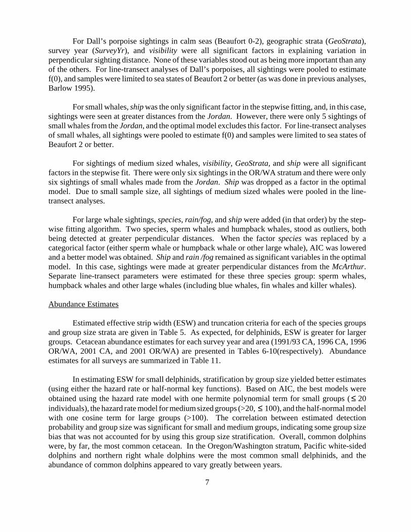
7
For Dall’s porpoise sightings in calm seas (Beaufort 0-2), geographic strata (GeoStrata),survey year (SurveyYr), and visibility were all significant factors in explaining variation inperpendicular sighting distance. None of these variables stood out as being more important than anyof the others. For line-transect analyses of Dall’s porpoises, all sightings were pooled to estimatef(0), and samples were limited to sea states of Beaufort 2 or better (as was done in previous analyses,Barlow 1995).
For small whales, ship was the only significant factor in the stepwise fitting, and, in this case,sightings were seen at greater distances from the Jordan. However, there were only 5 sightings ofsmall whales from the Jordan, and the optimal model excludes this factor. For line-transect analysesof small whales, all sightings were pooled to estimate f(0) and samples were limited to sea states ofBeaufort 2 or better.
For sightings of medium sized whales, visibility, GeoStrata, and ship were all significantfactors in the stepwise fit. There were only six sightings in the OR/WA stratum and there were onlysix sightings of small whales made from the Jordan. Ship was dropped as a factor in the optimalmodel. Due to small sample size, all sightings of medium sized whales were pooled in the line-transect analyses.
For large whale sightings, species, rain/fog, and ship were added (in that order) by the step-wise fitting algorithm. Two species, sperm whales and humpback whales, stood as outliers, bothbeing detected at greater perpendicular distances. When the factor species was replaced by acategorical factor (either sperm whale or humpback whale or other large whale), AIC was loweredand a better model was obtained. Ship and rain /fog remained as significant variables in the optimalmodel. In this case, sightings were made at greater perpendicular distances from the McArthur.Separate line-transect parameters were estimated for these three species group: sperm whales,humpback whales and other large whales (including blue whales, fin whales and killer whales).
Abundance Estimates
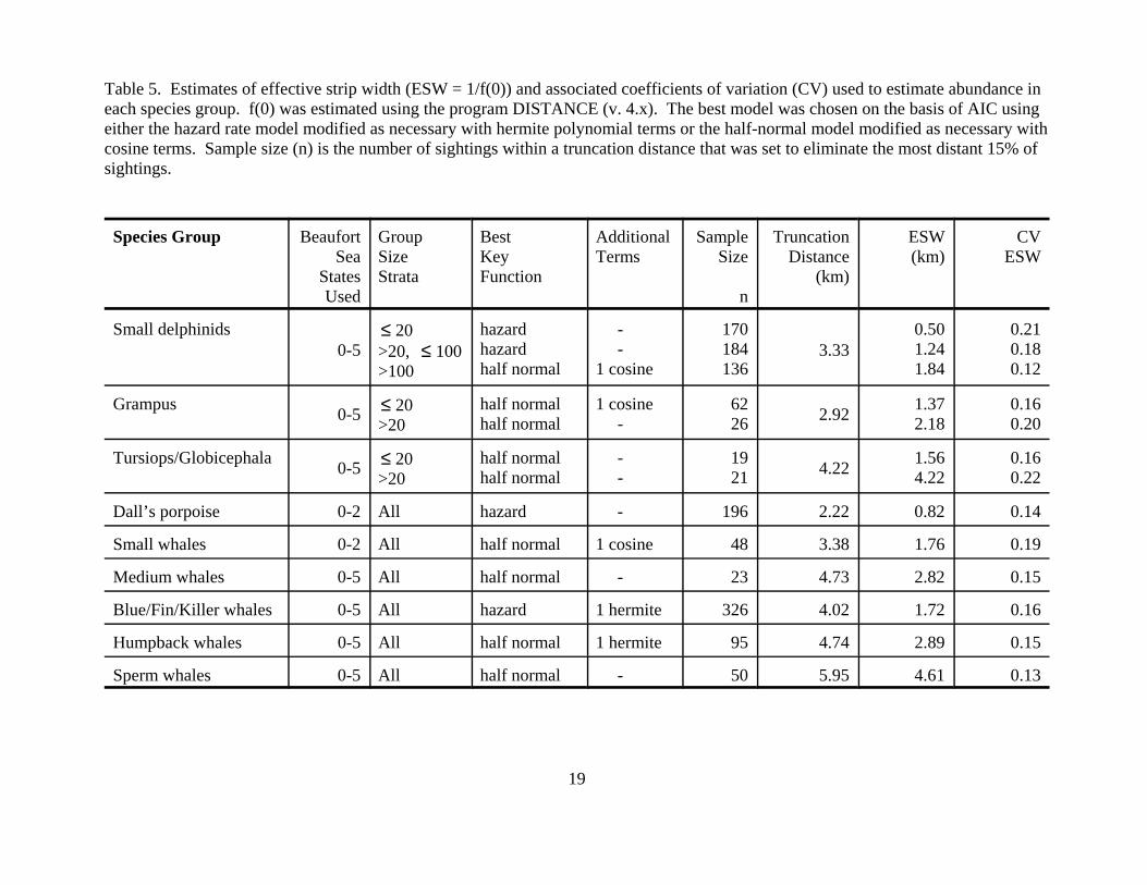
Estimated effective strip width (ESW) and truncation criteria for each of the species groupsand group size strata are given in Table 5. As expected, for delphinids, ESW is greater for largergroups. Cetacean abundance estimates for each survey year and area (1991/93 CA, 1996 CA, 1996OR/WA, 2001 CA, and 2001 OR/WA) are presented in Tables 6-10(respectively). Abundanceestimates for all surveys are summarized in Table 11.
In estimating ESW for small delphinids, stratification by group size yielded better estimates(using either the hazard rate or half-normal key functions). Based on AIC, the best models wereobtained using the hazard rate model with one hermite polynomial term for small groups ( 20≤individuals), the hazard rate model for medium sized groups (>20, 100), and the half-normal model≤with one cosine term for large groups (>100). The correlation between estimated detectionprobability and group size was significant for small and medium groups, indicating some group sizebias that was not accounted for by using this group size stratification. Overall, common dolphinswere, by far, the most common cetacean. In the Oregon/Washington stratum, Pacific white-sideddolphins and northern right whale dolphins were the most common small delphinids, and theabundance of common dolphins appeared to vary greatly between years.

8
Stratification by group size also resulted in better estimates of ESW for large delphinids(Grampus and Tursiops/Globicephala). The best detection model used the half-normal function withone cosine term for smaller groups ( 20) of Risso’s dolphins and the half-normal function for all≤other categories. The most common large delphinids in the California stratum were bottlenosedolphins and Risso’s dolphins. In the Oregon/Washington stratum, only Risso’s dolphins werecommon. Pilot whales were seen only during the 1991/93 and 1996 surveys.
For Dall’s porpoise, abundance estimates were based only on search effort in calm seas toensure that animals were detected before they reacted to the vessel. Even under these goodconditions, the effective strip width was only 820 m (Table 5). The hazard rate model gave the bestfit to the sighting distribution for this species. Given the precision of the estimates, abundanceappeared to be relatively constant among surveys in the California stratum but varied by almost anorder of magnitude in the Oregon/Washington stratum (Table 1 ). The distribution of search effortin calm seas was not geographically uniform in 1996 or 2001, and this probably contributes to theamong year variation seen in abundance estimates for Dall’s porpoise.
The estimates of abundance for small whales were similarly based only on effort in calm seas.The half-normal key function with one cosine term gave the best fit for this species group. Beakedwhales appeared more common in 1991/93 for both the common genera (7 sightings of Mesoplodonand 13 sightings of Ziphius). In 1996, there were only 3 sightings of Mesoplodon and two of Ziphius,and in 2001 Mesoplodon was not seen and there was only one sighting of Ziphius. Dwarf and pygmysperm whales (Kogia spp.) were not seen in 2001. Minke whales were seen in each survey year andtheir abundance estimates did not appear to fluctuate as much as the other species in this group.
The medium sized whales were the species group with the smallest number of total sightings(23 within the truncation distance of 4.7 km). All sightings were pooled, and the best fit to theirsighting distributions was obtained with a half-normal model. Bryde’s and sei whales remainedextremely rare in the study area throughout all survey years. The abundance of Baird’s beakedwhales, like that of smaller beaked whales, appeared to decline during the study period (Table 11).
The a priori category of large whales was split into three sub-categories for the purpose ofestimating line-transect parameters. Of these groups, the effective strip width was least for blue, finand killer whales, was intermediate for humpback whales, and was greatest for sperm whales. Thebest detection model was different for each group (Table 5). The estimated abundance of fin whalesincreased monotonically during the three survey periods, but the abundance of all other speciesshowed patterns that included both ups and downs. Killer whale abundance in theOregon/Washington stratum appeared comparable to or greater than that in the larger Californiastratum.
DiscussionPrevious Abundance Estimates
Estimates presented here differ, typically by a small amount, from previous estimates fromthe 1991, 1993, and 1996 surveys (Barlow 1995; Barlow and Gerrodette 1996; Barlow 1997). Thedifferences are primarily due to differences in the stratification and species groupings used forestimating ESW. The ability to pool samples from several surveys results in a larger sample size for

9
estimating of ESW and allowed stratification by other factors (including more species groups). Bothshould result in more precise estimates of cetacean abundance. Also, the estimates of Barlow (1997)did not include group size calibration for individual observers, and therefore the present estimatesfor the 1996 survey should have corrected a small negative bias present in those earlier estimates.The estimates presented here are expected to be more precise and less biased than previous estimates.The greater precision is not necessarily reflected in lower CVs because CVs are often not estimatedvery accurately.
Delphinids
Delphinids off the U.S. west coast can be classified as either warm-temperate to tropical(short- and long-beaked common dolphins, striped dolphins, bottlenose dolphins, and short-finnedpilot whales), cold-temperate (Pacific white-sided dolphins and northern right whale dolphins), orcosmopolitan (Risso’s dolphin and killer whales). The abundance of two warm-water species (short-beaked common dolphins and striped dolphins) appeared lower in 1996 than in 1991/93 or 2001.Two other warm-water species exhibited the opposite pattern (long-beaked common dolphins andbottlenose dolphins), but in both of those cases, the high abundance estimate and high CV in 1996was probably the result of the chance observation of a few very large groups. The cold-temperatespecies were more abundant in 1996. The cosmopolitan species did not vary much in abundanceamong years. The shifting patterns of warm and cold temperate species matches the seasonal changesin distributions seen for these species (Forney and Barlow 1998).
Dall’s Porpoise
Abundance estimation for Dall’s porpoise is difficult due to their attraction to vessels. Toobtain unbiased estimates, these animals must be detected before they react to the survey vessel. Ourdata indicate that the behavior of the vast majority of Dall’s porpoise seen at low sea states is “slowrolling”. This contrasts with the “rooster-tailing” or fast swimming behavior seen by animals thatare approaching the ship. However, limiting effort to calm conditions (Beaufort 2 and better) limitsthe number of sightings and, more importantly, limits effort to transect lines that are notgeographically uniform (Fig. 1). As a result, the coefficients of variation for Dall’s porpoiseabundance are greater than would be expected for the relatively large number of sightings. Thetemporal pattern shows higher Dall’s porpoise abundance in 1996, mirroring the higher abundancethat year of other cold-temperate delphinids (see above); however, given the lack of precision andthe lack of uniform geographic coverage, this pattern may be entirely coincidental.
Baleen Whales
The common baleen whales in California waters are blue, fin, and humpback whales. Theabundance of these species is consistently high during this study period. More precise estimates ofhumpback whale abundance are available from mark-recapture studies (Calambokidis et al. 2002),and these data indicate an increase in abundance through most of the 1990s followed by a decrease.The same pattern is found in my abundance estimates, but with less precision and no statisticallysignificant indication of a pattern. Estimates of blue whale abundance decreased markedly in 2001

10
compared to previous estimates. In the same year, Calambokidis et al. (2002) found that blue whaleswere very concentrated in California waters facilitating the collection of many identificationphotographs. This difference in perceived density of blue whales in 2001 may have been an artifactof their greater concentration; if whales were concentrated in one area, they could be easier to workfor photo-identification, but such areas might be missed by chance on a random line-transect survey.Fin whales appear to be monotonically increasing in abundance during the three survey periods, anda more detailed study of trends in fin whale abundance would be warranted (possibly including anearlier 1979/80 survey as well).
After nearly a decade of survey effort, it is now clear that Bryde’s and sei whales are notcommon off the U.S. west coast and that minke whale density is also low compared to other minkewhale habitats. Bryde’s whales are commonly viewed as tropical baleen whales, so their lowabundance is expected. However, sei whales were previously harvested commercially in the regionby coastal whaling stations, and their near absence is more of a mystery.
Sperm Whales
The abundance of sperm whales is more variable than that of the other large whales withsimilar population sizes. There may be several reasons for this. The most obvious is that spermwhales occur in larger groups and fewer groups are seen on each survey. High group size variationand low numbers of groups both contribute to higher CVs. Also, the sperm whale population is likelyto extend outside the study area, at least during some times of year. Sperm whales that were markedoff southern California in winter were later recovered by whalers north of the study area. It is likelythat at least some fraction of the population is absent during part of the year, and that fraction mayvary with oceanographic conditions. This differs from the situation with humpback and blue whalesfor which the majority of the population is believed to be feeding in U.S. west coast waters duringthe time of the surveys.
Beaked Whales
The apparent pattern of decreasing beaked whale abundance for all the common genera(Mesoplodon, Ziphius, and Berardius) is disconcerting, especially in light of recent discoveries aboutthe susceptibility of this group to loud anthropogenic sounds (Anon. 2001, Simmonds and Lopez-Jurado 1991). However, sea states during the 1996 and 2001 surveys were rougher than in 1991/93which could contribute to an apparent decline. Also, the geographic coverage in calm seas is notuniform, especially in later years. The distribution of all species extends outside the study area, andit is likely that some individuals move in and out of the study area based on habitat changes. Anaccurate analysis of trends in beaked whale abundance would have to include consideration of theseeffects. It is possible that sightings at higher sea states could also be used in an analysis of beakedwhale trends if the relative sighting efficiencies in different conditions could be included as acovariate.
Future Research
The results presented here are preliminary and will be improved by future analyses. TheGAMs analyses showed that many factors other than species, Beaufort, and group size can affect

11
perpendicular sighting distance. For example, ship appeared several times as a significant factor,with sightings being made at greater average distance from the McArthur than from the Jordan.GeoStrata and year were also significant for some species groups. Line-transect abundance estimatescan be improved by incorporating these factors as covariates when estimating ESW (Forcada 2002).The methods used in this paper are dependent on “pooling robustness”, and pooled estimates shouldbe unbiased, but estimates that are stratified by geographic region or year may be biased. Precisioncan likely be improved by using covariate models. Existing software for such analyses does notpermit stratification by species and geographic area, so custom software will have to be written tofacilitate such analyses.
The estimates of g(0) used here to account for perception bias for most species are based onindependent observer data from 1991 only. Additional data have been collected in subsequent yearsand could be used to improve estimates of g(0) for many species. Also, acoustic data on theprobability of detecting sperm whales have been collected on recent SWFSC surveys and could beused to improve estimates of g(0) for sperm whales to account for both perception and availabilitybias.
Acknowledgments
I thank the marine mammal observers (W. Armstrong, L. Baraff, S. Benson, J. Cotton, D.Everhardt, G. Friedrichsen, D. Kinzey, E. LaBrecque, H. Lira, M. Lycan, R. Mellon, S. Miller, L.Mitchell, L. Morse, S. Norman, P. Olson, S. Perry, J. Peterson, R. Pitman, T. Pusser, J. Quan, C.Speck, S. Rankin, K. Raum-Suryan, J. Rivers, R. Rowlett, J. C. Salinas, B. Smith, C. Stinchcomb,and L. Torres), cruise leaders (L. Ballance, J. Carretta, K. Forney, T. Gerrodette, P. S. Hill, M.Lowry, K. Mangels, S. Mesnick, R. Pitman, B. Taylor, and P. Wade), survey coordinators (J. Appler,P. S. Hill, A. Lynch, K. Mangels, A. VonSaunder), officers and crew who dedicated many monthsof hard work for these data. Tim Gerrodette was the chief scientist for the 1993 survey. This paperbenefitted from the reviews and comments by Megan Ferguson and the Pacific Scientific ReviewGroup.
12
Literature Cited
Anon. 2001. Joint interim report Bahamas marine mammal stranding event of 15-16 March 2000.Unpublished Report released by the U.S. Department of Commerce and the Secretary of theNavy. http://www.nmfs.noaa.gov/prot_res/overview/Interim_Bahamas_Report.pdf]. 59pp.
Barlow, J. 1988. Harbor porpoise (Phocoena phocoena) abundance estimation in California,Oregon and Washington: I. Ship surveys. Fish. Bull. 86:417-432.
Barlow, J. 1994. Abundance of large whales in California coastal waters: a comparison of shipsurveys in 1979/80 and in 1991. Rept. Int. Whal. Commn. 44:399-406.
Barlow, J. 1995. The abundance of cetaceans in California waters. Part I: Ship surveys in summerand fall of 1991. Fish. Bull. 93:1-14
Barlow, J. 1997. Preliminary estimates of cetacean abundance off California, Oregon, andWashington based on a 1996 ship survey and comparisons of passing and closing modes. Southwest Fisheries Science Center Administrative Report LJ-97-11. 25pp.
Barlow, J. 1999. Trackline detection probability for long-diving whales. pp. 209-221 In: G. W.Garner, et al. (eds.), Marine Mammal Survey and Assessment Methods. Balkema Press,Netherlands. 287pp.
Barlow, J. and K. A. Forney. 1994. An assessment of the 1994 status of harbor porpoise inCalifornia. NOAA Technical Memorandum NOAA-TM-NMFS-SWFSC-205. 17pp.
Barlow, J. and T. Gerrodette. 1996. Abundance of cetaceans in California waters based on 1991and 1993 ship surveys. NOAA Technical Memorandum NOAA-TM-NMFS-SWFSC-233. 15pp.
Barlow, J., T. Gerrodette, and J. Forcada. 2001. Factors affecting perpendicular sightingdistances on shipboard line-transect surveys for cetaceans. J. Cetacean Res. and Manage.3(2):201-212.
Barlow, J. T. Gerrodette, and W. Perryman. 1998. Calibrating group size estimates for cetaceansseen on ship surveys. Admin. Rept. LJ-98-11 available from Southwest Fisheries ScienceCenter, P.O. Box 271, La Jolla, CA. 39pp.
Barlow, J., C. Oliver, T. D. Jackson, and B. L. Taylor. 1988. Harbor porpoise (Phocoenaphocoena) abundance estimation in California, Oregon and Washington: II. Aerialsurveys. Fish. Bull. 86:433-444.
Barlow, J. and B. L. Taylor. 2001. Estimates of large whale abundance off California, Oregon,Washington, and Baja California based on 1993 and 1996 ship surveys. NOAA NationalMarine Fisheries Service, Southwest Fisheries Science Center Administrative Report

13
LJ-01-03.
Brueggeman, J. J., G. A. Green, K. C. Balcomb, C. E. Bowlby, R. A. Grotefendt, K. T. Briggs,M. L. Bonnell, R. G. Ford, D. H. Varoujean, D. Heinemann, and D. G. Chapman. 1990. Oregon-Washington Marine Mammal and Seabird Survey: Information synthesis andhypothesis formulation. U.S. Department of the Interior, OCS Study MMS 89-0030.
Buckland, S. T., D. R. Anderson, K. P. Burnham, and J. L. Laake. 1993a. Distance Sampling: Estimating abundance of biological populations. Chapman and Hall. London. 446pp.
Buckland, S. T., J. M. Breiwick, K. L. Cattanach, and J. L. Laake. 1993b. Estimated populationsize of the California gray whale. Mar. Mamm. Sci. 9(3):235-249.
Calambokidis, J., J. C. Cubbage, J. R. Evenson, S. D. Osmek, J. L. Laake, P. J. Gearin, B. J.Turnock, S. J. Jeffries, and R. F. Brown. 1993. Abundance estimates of harbor porpoisein Washington and Oregon waters. Final Contract Rept. #40ABNF201935 available fromNational Marine Mammal Laboratory. 55pp.
Calambokidis, J., T. Chandler, L. Schlender, K. Rasmussen, and G. Steiger. 2002. Research onhumpback and blue whales off California, Oregon and Washington in 2001. DraftContract Report to Southwest Fisheries Science Center, 8604 La Jolla Shores Dr., La JollaCA 92037.
Carretta, J. V., K. A. Forney, and J. L. Laake. 1998. Abundance of southern California coastalbottlenose dolphins estimated from tandem aerial surveys. Mar. Mamm. Sci. 14(4):655-675.
Dohl, T. P., M. L. Bonnell, And R. G. Ford. 1986. Distribution and abundance of commondolphin, Delphinus delphis, in the Southern California Bight: A quantitative assessmentbased on aerial transect data. Fish. Bull. 84:333-343.
Dohl, T. P., R. C. Guess, M. L. Duman, and R. C. Helm. 1983. Cetaceans of central andnorthern California, 1980-83: Status, abundance, and distribution. Final report to theMinerals Management Service, Contract No. 14-12-0001-29090. 284p.
Dohl, T. P., K. S. Norris, R. C. Guess, J. D. Bryant, and M. W. Honig. 1980. Cetacea of theSouthern California Bight. Part II of summary of marine mammals and seabird surveys ofthe Southern California Bight Area, 1975-78. Final Report to the Bureau of LandManagement, 414p. NTIS Rep. No. PB81248189.
Forcada, J. 2002. Multivariate methods for size-dependent detection in conventional linetransect sampling. SWFSC Admin. Rep., La Jolla, LJ-02-07, 35 p.
Forney, K.A. and J. Barlow. 1998 Seasonal patterns in the abundance and distribution ofCalifornia cetaceans, 1991-92. Mar.Mamm.Sci. 14(3):460-489.

14
Forney, K. A., Barlow, J., and J. V. Carretta. 1995. The abundance of cetaceans in Californiawaters. Part II: Aerial surveys in winter and spring of 1991 and 1992. Fish. Bull. 93:15-26.
Gerrodette, T., W. Perryman and J. Barlow. 2002. Calibrating group size estimates of dolphinsin the eastern tropical Pacific Ocean. Administrative Report LJ-02-08, available fromSouthwest Fisheries Science Center, P.O. Box 271, La Jolla, CA 92038. 73pp.
Hill, P. S. and J. Barlow. 1992. Report of a marine mammal survey of the California coastaboard the research vessel McARTHUR July 28-November 5, 1991. NOAA TechnicalMemorandum NOAA-TM-NMFS-SWFSC-169. NTIS #PB93-109908. 103pp.
Mangels, K. F. and T. Gerrodette. 1994. Report of cetacean sightings during a marine mammalsurvey in the eastern Pacific Ocean and the Gulf of California aboard the NOAA shipsMcArthur and David Starr Jordan July 28 - November 6, 1993. NOAA TechnicalMemorandum NOAA-TM-NMFS-SWFSC-211. 86pp.
Reilly, S. B. 1984. Observed and maximum rates of increase in gray whales, Eschrichtiusrobustus. Rep. Int. Whal. Commn. Special Issue 6:389-399.
Simmonds, M. P. and L. F. Lopez-Jurado. 1991. Whales and the military. Nature 51:448.
Von Saunder, A. and J. Barlow. 1999. A report of the Oregon, California and Washington Line-transect Experiment (ORCAWALE) conducted in west coast waters during summer/fall1996. NOAA Tech. Mem. NOAA-TM-NMFS-SWFSC-264. 40pp.

15
Table 1. Survey dates, ships used, and areas surveyed.
Survey Ship Dates Area
CAMMS-91 McArthur 28 Jul. - 05 Nov. 1991 California
PODS-93 McArthur 28 Jul. - 06 Nov. 1993 California
ORCAWALE-96 McArthurJordan
17 Jul.- 14 Oct. 199604 Sep.-06 Nov. 1996
California/Oregon/Washington
ORCAWALE-01 McArthurJordan
30 Jul. - 08 Dec. 2001 California/Oregon/Washington
16
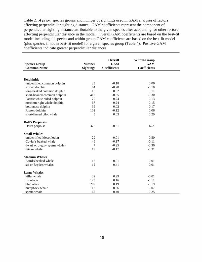
Table 2. A priori species groups and number of sightings used in GAM analyses of factorsaffecting perpendicular sighting distance. GAM coefficients represent the component ofperpendicular sighting distance attributable to the given species after accounting for other factorsaffecting perpendicular distance in the model. Overall GAM coefficients are based on the best-fitmodel including all species and within-group GAM coefficients are based on the best-fit model(plus species, if not in best-fit model) for a given species group (Table 4). Positive GAMcoefficients indicate greater perpendicular distances.
Overall Within-Group Species Group Number GAM GAM Common Name Sightings Coefficients Coefficients
Delphinids unidentified common dolphin 23 -0.18 0.06 striped dolphin 64 -0.28 -0.10 long-beaked common dolphin 15 0.02 0.11 short-beaked common dolphin 412 -0.35 -0.30 Pacific white-sided dolphin 70 -0.24 -0.13 northern right whale dolphin 67 -0.24 -0.15 bottlenose dolphin 39 0.02 0.17 Risso's dolphin 102 -0.12 0.06 short-finned pilot whale 5 0.03 0.29
Dall’s Porpoises Dall's porpoise 376 -0.31 N/A
Small Whales unidentified Mesoplodon 29 -0.01 0.50 Cuvier's beaked whale 46 -0.17 -0.11 dwarf or pygmy sperm whales 7 -0.25 -0.36 minke whale 19 -0.17 -0.31
Medium Whales Baird's beaked whale 15 -0.01 0.01 sei or Bryde's whales 12 0.41 -0.01
Large Whales killer whale 22 0.29 -0.01 fin whale 173 0.16 -0.11 blue whale 202 0.19 -0.19 humpback whale 113 0.36 0.07 sperm whale 62 0.40 0.25

17
Table 3. Regression coefficients, , estimated for the indirect calibration of group size basedβ0
on a comparison of an individual observer’s “best” estimates of group size with the meancalibrated group size estimated from two or more other “calibrated” observers for all yearspooled. ASPE indicates the average squared prediction error using this regression coefficient. Calibration coefficients for directly calibrated observers are given by Gerrodette et al. 2002.
Observer Sample Number Size ASPEβ0
077 58 0.984 .0849 088 61 0.822 .2945 104 125 0.887 .2281 138 27 0.903 .1550 143 41 0.943 .1764 145 45 0.898 .2377 148 23 1.005 .4293 154 23 0.947 .0902 201 85 0.886 .1970

18
Table 4. Factors included in generalized additive models that best estimate mean perpendiculardistance for a priori species groups. Factors are listed in the order they were added to the model(most significant factors first). Best-fit models are the lowest-AIC models obtained using astepwise fitting algorithm. Optimal models are the simplest models within 2 AIC units of thebest-fit models. Alternative species groupings were adopted for optimal models if the best-fitmodels included species as a significant factor and if a lower AIC value could be obtained. Numbers in parentheses after continuous variables are the number of terms in spline-fit models.
Species Group Factors AIC
Delphinids Best-fit Model GroupSize(4) + Beauf(2) + Species + Ship + Time 304.3 Optimal Model GroupSize(4) + RankBeauf + (Sm vs. Lg Delphinid) + Ship 301.8
Dall’s Porpoises (Beauf. <= 2) Best-fit Model GeoStrata + SurveyYr + Visibility 174.9 Optimal Model GeoStrata + SurveyYr + Visibility 174.9
Small Whales (Beauf. <= 2) Best-fit Model Ship 44.6 Optimal Model NULL 46.5
Medium Whales Best-fit Model Visibility + GeoStrata + Ship 13.0 Optimal Model Visibility + GeoStrata 14.0
Large Whales Best-fit Model Species + RainFog + Ship 302.4 Optimal Model (Sperm whale vs. Humpback vs. Others) + RainFog + Ship 301.3
19
Table 5. Estimates of effective strip width (ESW = 1/f(0)) and associated coefficients of variation (CV) used to estimate abundance ineach species group. f(0) was estimated using the program DISTANCE (v. 4.x). The best model was chosen on the basis of AIC usingeither the hazard rate model modified as necessary with hermite polynomial terms or the half-normal model modified as necessary withcosine terms. Sample size (n) is the number of sightings within a truncation distance that was set to eliminate the most distant 15% ofsightings.
Species Group BeaufortSea
StatesUsed
GroupSizeStrata
BestKeyFunction
AdditionalTerms
SampleSize
n
TruncationDistance
(km)
ESW(km)
CVESW
Small delphinids0-5
20≤>20, 100≤>100
hazardhazardhalf normal
- -1 cosine
170184136
3.330.501.241.84
0.210.180.12
Grampus 0-5 20≤>20
half normalhalf normal
1 cosine -
6226 2.92 1.37
2.180.160.20
Tursiops/Globicephala 0-5 20≤>20
half normalhalf normal
- -
1921 4.22 1.56
4.220.160.22
Dall’s porpoise 0-2 All hazard - 196 2.22 0.82 0.14
Small whales 0-2 All half normal 1 cosine 48 3.38 1.76 0.19
Medium whales 0-5 All half normal - 23 4.73 2.82 0.15
Blue/Fin/Killer whales 0-5 All hazard 1 hermite 326 4.02 1.72 0.16
Humpback whales 0-5 All half normal 1 hermite 95 4.74 2.89 0.15
Sperm whales 0-5 All half normal - 50 5.95 4.61 0.13
20
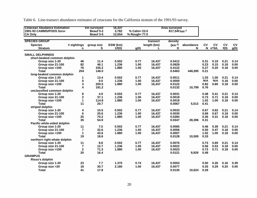
Area surveyed16,437km surveyedCetacean Abudance Estimationkm-2817,54923.0% Calm=3,782Beauf 0-21991-93 CAMMS/PODS Surve
77.0% Rough=12,654Beauf 3-5CA Only
densitytransectSPECIES GROUPCVCVCVCVabundance (km-2)length (km)ESW (km)group size# sightingsSpecies
g(0)f(0)n*S/LNNDLg(0)1/f(0)SnStratum
SMALL DELPHINIDSshort-beaked common dolphin
0.140.210.190.310.041216,4370.770.50211.446Group size 1-200.000.180.150.230.092916,4371.001.23646.182Group size 21-1000.000.180.200.270.412216,4371.001.880335.276Group size >100
0.21446,5950.5463146.0204Totallong-beaked common dolphin
0.140.211.001.030.001116,4370.770.50213.41Group size 1-200.000.18N/AN/A0.000016,4371.001.2360.00Group size 21-1000.000.180.800.820.012216,4371.001.880250.53Group size >100
0.7610,7990.0132191.24Totalunclassified common dolphin
0.140.210.410.480.003116,4370.770.5024.98Group size 1-200.000.180.710.730.001816,4371.001.23637.12Group size 21-1000.000.181.001.020.001916,4371.001.880114.81Group size >100
0.415,5130.006720.711Totalstriped dolphin
0.140.210.620.670.003316,4370.770.50210.54Group size 1-200.000.180.670.690.003016,4371.001.23620.66Group size 21-1000.000.180.310.360.028416,4371.001.88070.225Group size >100
0.3128,3960.034754.935TotalPacific white-sided dolphin
0.140.210.390.460.006516,4370.770.5027.511Group size 1-200.000.180.470.500.005616,4371.001.23632.67Group size 21-1000.000.181.001.020.000716,4371.001.88043.61Group size >100
0.3310,5000.012818.619Totalnorthern right whale dolphin
0.140.210.690.730.007616,4370.770.5028.811Group size 1-200.000.180.530.560.002216,4371.001.23612.77Group size 21-1000.000.180.710.730.002316,4371.001.88071.32Group size >100
0.499,9290.012116.420TotalGRAMPUS
Risso's dolphin0.390.160.260.500.005316,4370.741.3707.723Group size 1-200.000.200.290.350.007716,4371.002.18030.718Group size >20
0.2910,6240.013017.841Total
Table 6. Line-transect abundance estimates of cetaceans for the California stratum of the 1991/93 survey.

21
TURSIOPS/GLOBICEPHALAbottlenose dolphin
0.390.160.620.750.000416,4370.741.5603.45Group size 1-200.000.220.350.410.001116,4371.004.22013.012Group size >20
0.361,2820.001610.217Totalpilot whale
0.390.160.710.830.000616,4370.741.56011.52Group size 1-200.000.220.710.740.000316,4371.004.22018.52Group size >20
0.627130.000915.04TotalDALL'S PORPOISE
Dall's porpoise0.100.140.260.3131,3960.03843,7820.790.8193.258Calm Seas
SMALL WHALESziphiid whale
0.290.190.710.795300.00063,7820.341.7641.52Calm SeasMesoplodon spp.
0.230.190.380.481,6680.00203,7820.451.7641.87Calm SeasCuvier's beaked whale
0.350.190.300.508,3110.01023,7820.231.7642.413Calm SeasKogia spp.
0.290.190.360.507000.00093,7820.351.7641.04Calm Seasminke whale
0.220.190.330.442210.00033,7820.841.7641.03Calm SeasMEDIUM WHALES
Baird's beaked whale0.230.150.550.617650.000916,4370.962.82513.96Total
Bryde's whale0.070.151.001.01200.000016,4370.902.8252.01Total
sei whale0.070.150.770.79400.000016,4370.902.8251.43Total
sei/Bryde's whale0.070.150.500.53490.000116,4370.902.8251.05Total
LARGE WHALESkiller whale
0.070.160.470.504540.000616,4370.901.7155.65Totalfin whale
0.070.160.300.351,6350.002016,4370.901.7152.051Totalblue whale
0.070.160.170.242,7130.003316,4370.901.7151.892TotalHUMPBACK WHALE
humpback whale0.070.150.370.415510.000716,4370.902.8942.226Total
SPERM WHALEsperm whale
0.080.130.370.401,1680.001416,4370.874.6076.728Total
Table 6. (Continued).

22
Area surveyed10,401km surveyedCetacean Abudance Estimationkm-2817,54915.2% Calm=1,579Beauf 0-21996 ORCAWALE Survey
84.8% Rough=8,821Beauf 3-5CA Only
densitytransectSPECIES GROUPCVCVCVCVabundance (km-2)length (km)ESW (km)group size# sightingsSpecies
g(0)f(0)n*S/LNNDLg(0)1/f(0)SnStratum
SMALL DELPHINIDSshort-beaked common dolphin
0.140.210.290.380.031110,4010.770.50211.921Group size 1-200.000.180.300.350.063610,4011.001.23648.134Group size 21-1000.000.180.230.290.365310,4011.001.880348.441Group size >100
0.24376,0400.4600168.496Totallong-beaked common dolphin
0.140.211.001.030.001910,4010.770.50215.21Group size 1-200.000.181.001.020.000910,4011.001.23622.11Group size 21-1000.000.180.720.740.103010,4011.001.8801006.64Group size >100
0.7286,4140.1057677.36Totalunclassified common dolphin
0.140.210.500.560.006610,4010.770.5028.86Group size 1-200.000.180.710.730.002110,4011.001.23627.32Group size 21-1000.000.180.710.730.001010,4011.001.88018.92Group size >100
0.427,9060.009714.510Totalstriped dolphin
0.140.211.001.030.000210,4010.770.5022.01Group size 1-200.000.180.710.730.004210,4011.001.23653.52Group size 21-1000.000.180.440.470.002310,4011.001.88011.38Group size >100
0.485,4890.006718.111TotalPacific white-sided dolphin
0.140.210.650.700.005510,4010.770.5028.95Group size 1-200.000.180.430.460.016210,4011.001.23652.28Group size 21-1000.000.180.870.890.079810,4011.001.880520.16Group size >100
0.7083,0320.1016188.619Totalnorthern right whale dolphin
0.140.211.001.030.000610,4010.770.5024.71Group size 1-200.000.180.770.790.002810,4011.001.23624.03Group size 21-1000.000.180.640.660.014510,4011.001.880113.15Group size >100
0.5514,5930.017871.49TotalGRAMPUS
Risso's dolphin0.390.160.400.580.003610,4010.741.3707.710Group size 1-200.000.200.670.700.007010,4011.002.18063.25Group size >20
0.508,6720.010626.215Total
Table 7. Line-transect abundance estimates of cetaceans for the California stratum of the 1996 survey.

23
TURSIOPS/GLOBICEPHALAbottlenose dolphin
0.390.160.650.770.000410,4010.741.5602.74Group size 1-200.000.221.101.120.006210,4011.004.220109.55Group size >20
1.055,4640.006762.09Totalpilot whale
0.390.16N/AN/A0.000010,4010.741.5600.00Group size 1-200.000.221.001.020.000710,4011.004.22065.31Group size >20
1.026080.000765.31TotalDALL'S PORPOISE
Dall's porpoise0.100.140.530.5670,2070.08591,5790.790.8193.353Calm Seas
SMALL WHALESziphiid whale
0.290.191.001.068630.00111,5790.341.7641.02Calm SeasMesoplodon spp.
0.230.191.001.043260.00041,5790.451.7641.01Calm SeasCuvier's beaked whale
0.350.190.710.811,8760.00231,5790.231.7641.52Calm SeasKogia spp.
0.290.19N/AN/A00.00001,5790.351.7640.00Calm Seasminke whale
0.220.190.420.517760.00091,5790.841.7641.14Calm SeasMEDIUM WHALES
Baird's beaked whale0.230.150.710.762750.000310,4010.962.8259.52Total
Bryde's whale0.070.15N/AN/A00.000010,4010.902.8250.00Total
sei whale0.070.150.710.73860.000110,4010.902.8252.82Total
sei/Bryde's whale0.070.15N/AN/A00.000010,4010.902.8250.00Total
LARGE WHALESkiller whale
0.070.160.580.616130.000710,4010.901.7156.04Totalfin whale
0.070.160.290.342,6380.003210,4010.901.7151.956Totalblue whale
0.070.160.220.282,5840.003210,4010.901.7151.473TotalHUMPBACK WHALE
humpback whale0.070.150.410.441,5030.001810,4010.902.8941.953Total
SPERM WHALEsperm whale
0.080.130.540.563910.000510,4010.874.6074.49Total
Table 7. (Continued).

24
Area surveyed4,349km surveyedCetacean Abudance Estimationkm-2325,01812.3% Calm=533Beauf 0-21996 ORCAWALE Survey
87.7% Rough=3,816Beauf 3-5OR+WA Only
densitytransectSPECIES GROUPCVCVCVCVabundance (km-2)length (km)ESW (km)group size# sightingsSpecies
g(0)f(0)n*S/LNNDLg(0)1/f(0)SnStratum
SMALL DELPHINIDSshort-beaked common dolphin
0.140.21N/AN/A0.00004,3490.770.5020.00Group size 1-200.000.18N/AN/A0.00004,3491.001.2360.00Group size 21-1000.000.181.001.020.01944,3491.001.880317.81Group size >100
1.026,3160.0194317.81Totallong-beaked common dolphin
0.140.21N/AN/A0.00004,3490.770.5020.00Group size 1-200.000.18N/AN/A0.00004,3491.001.2360.00Group size 21-1000.000.18N/AN/A0.00004,3491.001.8800.00Group size >100
N/A00.00000.00Totalunclassified common dolphin
0.140.21N/AN/A0.00004,3490.770.5020.00Group size 1-200.000.18N/AN/A0.00004,3491.001.2360.00Group size 21-1000.000.18N/AN/A0.00004,3491.001.8800.00Group size >100
N/A00.00000.00Totalstriped dolphin
0.140.21N/AN/A0.00004,3490.770.5020.00Group size 1-200.000.18N/AN/A0.00004,3491.001.2360.00Group size 21-1000.000.181.001.020.00024,3491.001.8803.21Group size >100
1.02640.00023.21TotalPacific white-sided dolphin
0.140.211.001.030.00334,3490.770.50211.01Group size 1-200.000.180.710.730.00304,3491.001.23616.32Group size 21-1000.000.181.001.020.02044,3491.001.880333.91Group size >100
0.798,6830.026794.44Totalnorthern right whale dolphin
0.140.210.710.750.00444,3490.770.5027.42Group size 1-200.000.181.001.020.00194,3491.001.23620.31Group size 21-1000.000.180.710.730.00924,3491.001.88074.92Group size >100
0.505,0260.015537.05TotalGRAMPUS
Risso's dolphin0.390.160.560.700.00194,3490.741.3704.24Group size 1-200.000.200.700.730.02334,3491.002.18088.45Group size >20
0.688,1870.025250.99Total
Table 8. Line-transect abundance estimates of cetaceans for the Oregon/Washington stratum of the 1996 survey.

25
TURSIOPS/GLOBICEPHALAbottlenose dolphin
0.390.16N/AN/A0.00004,3490.741.5600.00Group size 1-200.000.22N/AN/A0.00004,3491.004.2200.00Group size >20
N/A00.00000.00Totalpilot whale
0.390.16N/AN/A0.00004,3490.741.5600.00Group size 1-200.000.22N/AN/A0.00004,3491.004.2200.00Group size >20
N/A00.00000.00TotalDALL'S PORPOISE
Dall's porpoise0.100.140.570.5976,8740.23655330.790.8193.448Calm Seas
SMALL WHALESziphiid whale
0.290.19N/AN/A00.00005330.341.7640.00Calm SeasMesoplodon spp.
0.230.191.001.042,1690.00675330.451.7642.82Calm SeasCuvier's beaked whale
0.350.19N/AN/A00.00005330.231.7640.00Calm SeasKogia spp.
0.290.191.001.064940.00155330.351.7641.01Calm Seasminke whale
0.220.190.710.774110.00135330.841.7641.02Calm SeasMEDIUM WHALES
Baird's beaked whale0.230.150.620.68640.00024,3490.962.8251.63Total
Bryde's whale0.070.15N/AN/A00.00004,3490.902.8250.00Total
sei whale0.070.15N/AN/A00.00004,3490.902.8250.00Total
sei/Bryde's whale0.070.15N/AN/A00.00004,3490.902.8250.00Total
LARGE WHALESkiller whale
0.070.160.660.684200.00134,3490.901.7155.83Totalfin whale
0.070.160.530.562830.00094,3490.901.7151.39Totalblue whale
0.070.16N/AN/A00.00004,3490.901.7150.00TotalHUMPBACK WHALE
humpback whale0.070.151.001.01150.00004,3490.902.8941.11Total
SPERM WHALEsperm whale
0.080.130.690.714400.00144,3490.874.60711.84Total
Table 8. (Continued).
26
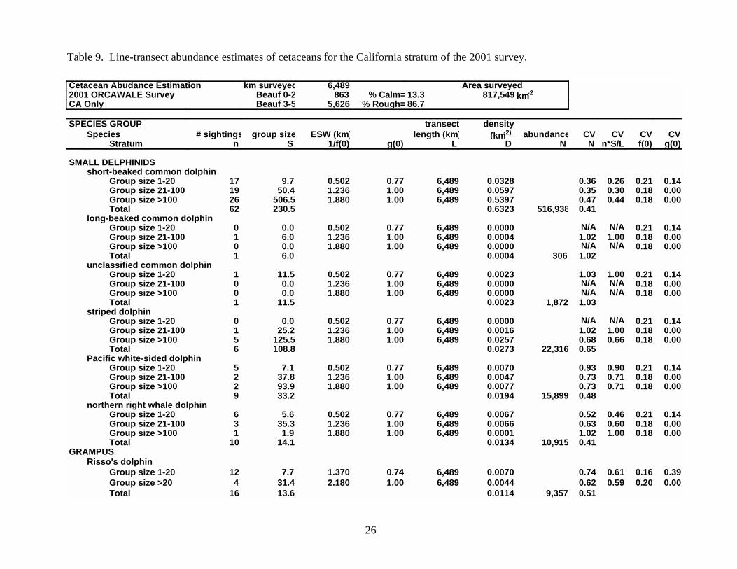
Area surveyed6,489km surveyedCetacean Abudance Estimationkm-2817,54913.3% Calm=863Beauf 0-22001 ORCAWALE Survey
86.7% Rough=5,626Beauf 3-5CA Only
densitytransectSPECIES GROUPCVCVCVCVabundance (km-2)length (km)ESW (km)group size# sightingsSpecies
g(0)f(0)n*S/LNNDLg(0)1/f(0)SnStratum
SMALL DELPHINIDSshort-beaked common dolphin
0.140.210.260.360.03286,4890.770.5029.717Group size 1-200.000.180.300.350.05976,4891.001.23650.419Group size 21-1000.000.180.440.470.53976,4891.001.880506.526Group size >100
0.41516,9380.6323230.562Totallong-beaked common dolphin
0.140.21N/AN/A0.00006,4890.770.5020.00Group size 1-200.000.181.001.020.00046,4891.001.2366.01Group size 21-1000.000.18N/AN/A0.00006,4891.001.8800.00Group size >100
1.023060.00046.01Totalunclassified common dolphin
0.140.211.001.030.00236,4890.770.50211.51Group size 1-200.000.18N/AN/A0.00006,4891.001.2360.00Group size 21-1000.000.18N/AN/A0.00006,4891.001.8800.00Group size >100
1.031,8720.002311.51Totalstriped dolphin
0.140.21N/AN/A0.00006,4890.770.5020.00Group size 1-200.000.181.001.020.00166,4891.001.23625.21Group size 21-1000.000.180.660.680.02576,4891.001.880125.55Group size >100
0.6522,3160.0273108.86TotalPacific white-sided dolphin
0.140.210.900.930.00706,4890.770.5027.15Group size 1-200.000.180.710.730.00476,4891.001.23637.82Group size 21-1000.000.180.710.730.00776,4891.001.88093.92Group size >100
0.4815,8990.019433.29Totalnorthern right whale dolphin
0.140.210.460.520.00676,4890.770.5025.66Group size 1-200.000.180.600.630.00666,4891.001.23635.33Group size 21-1000.000.181.001.020.00016,4891.001.8801.91Group size >100
0.4110,9150.013414.110TotalGRAMPUS
Risso's dolphin0.390.160.610.740.00706,4890.741.3707.712Group size 1-200.000.200.590.620.00446,4891.002.18031.44Group size >20
0.519,3570.011413.616Total
Table 9. Line-transect abundance estimates of cetaceans for the California stratum of the 2001 survey.

27
TURSIOPS/GLOBICEPHALAbottlenose dolphin
0.390.160.961.050.00366,4890.741.56010.85Group size 1-200.000.220.800.830.00216,4891.004.22028.84Group size >20
0.734,6660.005718.89Totalpilot whale
0.390.16N/AN/A0.00006,4890.741.5600.00Group size 1-200.000.22N/AN/A0.00006,4891.004.2200.00Group size >20
N/A00.00000.00TotalDALL'S PORPOISE
Dall's porpoise0.100.140.610.6341,9400.05138630.790.8192.325Calm Seas
SMALL WHALESziphiid whale
0.290.19N/AN/A00.00008630.341.7640.00Calm SeasMesoplodon spp.
0.230.19N/AN/A00.00008630.451.7640.00Calm SeasCuvier's beaked whale
0.350.191.001.081,8920.00238630.231.7641.61Calm SeasKogia spp.
0.290.19N/AN/A00.00008630.351.7640.00Calm Seasminke whale
0.220.190.710.777160.00098630.841.7641.12Calm SeasMEDIUM WHALES
Baird's beaked whale0.230.15N/AN/A00.00006,4890.962.8250.00Total
Bryde's whale0.070.15N/AN/A00.00006,4890.902.8250.00Total
sei whale0.070.151.001.01250.00006,4890.902.8251.01Total
sei/Bryde's whale0.070.15N/AN/A00.00006,4890.902.8250.00Total
LARGE WHALESkiller whale
0.070.160.710.734800.00066,4890.901.7155.92Totalfin whale
0.070.160.530.563,2570.00406,4890.901.7154.020Totalblue whale
0.070.160.400.447880.00106,4890.901.7151.910TotalHUMPBACK WHALE
humpback whale0.070.150.460.497430.00096,4890.902.8941.916Total
SPERM WHALEsperm whale
0.080.130.570.591,5810.00196,4890.874.60711.29Total
Table 9. (Continued).

28
Area surveyed3,133km surveyedCetacean Abudance Estimationkm-2325,01827.5% Calm=863Beauf 0-22001 ORCAWALE Survey
72.5% Rough=2,270Beauf 3-5OR+WA Only
densitytransectSPECIES GROUPCVCVCVCVabundance (km-2)length (km)ESW (km)group size# sightingsSpecies
g(0)f(0)n*S/LNNDLg(0)1/f(0)SnStratum
SMALL DELPHINIDSshort-beaked common dolphin
0.140.211.001.030.00123,1330.770.5023.01Group size 1-200.000.18N/AN/A0.00003,1331.001.2360.00Group size 21-1000.000.18N/AN/A0.00003,1331.001.8800.00Group size >100
1.033980.00123.01Totallong-beaked common dolphin
0.140.21N/AN/A0.00003,1330.770.5020.00Group size 1-200.000.18N/AN/A0.00003,1331.001.2360.00Group size 21-1000.000.18N/AN/A0.00003,1331.001.8800.00Group size >100
N/A00.00000.00TotalN/AN/Aunclassified common dolphin
0.140.21N/AN/A0.00003,1330.770.5020.00Group size 1-200.000.18N/AN/A0.00003,1331.001.2360.00Group size 21-1000.000.18N/AN/A0.00003,1331.001.8800.00Group size >100
N/A00.00000.00Totalstriped dolphin
0.140.21N/AN/A0.00003,1330.770.5020.00Group size 1-200.000.18N/AN/A0.00003,1331.001.2360.00Group size 21-1000.000.18N/AN/A0.00003,1331.001.8800.00Group size >100
N/A00.00000.00TotalPacific white-sided dolphin
0.140.210.570.620.01643,1330.770.50210.04Group size 1-200.000.180.710.730.00363,1331.001.23613.92Group size 21-1000.000.181.001.020.01363,1331.001.880160.41Group size >100
0.5210,9340.033632.67Totalnorthern right whale dolphin
0.140.210.510.570.02153,1330.770.5028.76Group size 1-200.000.180.730.750.00803,1331.001.23620.83Group size 21-1000.000.181.001.020.00183,1331.001.88020.91Group size >100
0.4410,1900.031413.510TotalGRAMPUS
Risso's dolphin0.390.160.560.700.01253,1330.741.37013.26Group size 1-200.000.200.710.740.00573,1331.002.18039.12Group size >20
0.535,9170.018219.78Total
Table 10 Line-transect abundance estimates of cetaceans for the Oregon/Washington stratum of the 2001 survey.

29
TURSIOPS/GLOBICEPHALAbottlenose dolphin
0.390.16N/AN/A0.00003,1330.741.5600.00Group size 1-200.000.22N/AN/A0.00003,1331.004.2200.00Group size >20
N/A00.00000.00Totalpilot whale
0.390.16N/AN/A0.00003,1330.741.5600.00Group size 1-200.000.22N/AN/A0.00003,1331.004.2200.00Group size >20
N/A00.00000.00TotalDALL'S PORPOISE
Dall's porpoise0.100.140.480.518,2130.02538630.790.8192.412Calm Seas
SMALL WHALESziphiid whale
0.290.19N/AN/A00.00008630.341.7640.00Calm SeasMesoplodon spp.
0.230.19N/AN/A00.00008630.451.7640.00Calm SeasCuvier's beaked whale
0.350.19N/AN/A00.00008630.231.7640.00Calm SeasKogia spp.
0.290.19N/AN/A00.00008630.351.7640.00Calm Seasminke whale
0.220.191.001.041270.00048630.841.7641.01Calm SeasMEDIUM WHALES
Baird's beaked whale0.230.150.710.761170.00043,1330.962.8253.12Total
Bryde's whale0.070.15N/AN/A00.00003,1330.902.8250.00Total
sei whale0.070.15N/AN/A00.00003,1330.902.8250.00Total
sei/Bryde's whale0.070.15N/AN/A00.00003,1330.902.8250.00Total
LARGE WHALESkiller whale
0.070.160.480.511,1670.00363,1330.901.7158.74Totalfin whale
0.070.160.480.513800.00123,1330.901.7151.110Totalblue whale
0.070.160.690.711010.00033,1330.901.7151.03TotalHUMPBACK WHALE
humpback whale0.070.150.420.453660.00113,1330.902.8942.38Total
SPERM WHALEsperm whale
0.080.130.710.73520.00023,1330.874.6072.02Total
Table 10. (Continued).

30
CA+OR+WAOregon+WashingtonCalifornia CA+OR+WACetacean Abudance Estimation
1996+20012001199620011996200119961991-93SPECIES GROUPAbundanceAbundanceAbundanceAbundanceAbundanceAbundanceAbundanceAbundanceSpecies
SMALL DELPHINIDS449,846517,335382,3563986,316516,938376,040446,595short-beaked common dolphin
0.250.410.231.031.020.410.240.21
43,36030686,4140030686,41410,799long-beaked common dolphin0.721.020.72N/AN/A1.020.720.76
4,8891,8727,906001,8727,9065,513unclassified common dolphin0.391.030.42N/AN/A1.030.420.41
13,93422,3165,55306422,3165,48928,396striped dolphin0.530.650.48N/A1.020.650.480.31
59,27426,83391,71510,9348,68315,89983,03210,500Pacific white-sided dolphin0.500.350.640.520.790.480.700.33
20,36221,10419,61910,1905,02610,91514,5939,929northern right whale dolphin0.260.300.430.440.500.410.550.49
GRAMPUS16,06615,27416,8585,9178,1879,3578,67210,624Risso's dolphin
0.280.380.420.530.680.510.500.29
TURSIOPS / GLOBICEPHALA5,0654,6665,464004,6665,4641,282bottlenose dolphin0.660.731.05N/AN/A0.731.050.36
3040608000608713pilot whale1.02N/A1.02N/AN/AN/A1.020.62
DALL'S PORPOISE98,61750,153147,0818,21376,87441,94070,20731,396Dall's porpoise
0.330.540.410.510.590.630.560.31SMALL WHALES
4320863000863530ziphiid whale1.06N/A1.06N/AN/AN/A1.060.79
1,24702,49502,16903261,668Mesoplodon spp.0.92N/A0.92N/A1.04N/A1.040.48
1,8841,8921,876001,8921,8768,311Cuvier's beaked whale0.681.080.81N/AN/A1.080.810.50
2470494049400700Kogia spp.1.06N/A1.06N/A1.06N/AN/A0.50
1,0158431,187127411716776221minke whale0.370.670.431.040.770.770.510.44
MEDIUM WHALES228117339117640275765Baird's beaked whale0.510.760.630.760.68N/A0.760.61
000000020Bryde's whaleN/AN/AN/AN/AN/AN/AN/A1.01
56258600258640sei whale0.611.010.73N/AN/A1.010.730.79
000000049sei/Bryde's whaleN/AN/AN/AN/AN/AN/AN/A0.53
LARGE WHALES1,3401,6471,0331,167420480613454killer whale0.310.420.450.510.680.730.610.50
3,2793,6362,9213802833,2572,6381,635fin whale0.310.500.310.510.560.560.340.35
1,7368882,58410107882,5842,713blue whale0.230.400.280.71N/A0.440.280.24
HUMPBACK WHALE1,3141,1091,518366157431,503551humpback whale0.300.360.440.451.010.490.440.41
SPERM WHALE1,2331,634831524401,5813911,168sperm whale0.410.570.460.730.710.590.560.40
Table 11. Summary of line-transect estimates of cetacean abundance and associated CVsstratified by year and geographic region.

31
Figure 1. Distribution of search effort within defined geographic strata (CA and OR/WA) during 1991/93, 1996, and 2001 surveys in Beaufort sea states 0-2 (left) and 0-5 (right).