Subpixel abundance estimates in mixture-tuned matched filtering ...

Subpixel abundance estimates in mixture-tuned matched filteringclassifications of leafy spurge (Euphorbia esula L.)

J. J. MITCHELL*† and N. F. GLENN‡

†Department of Geosciences, Idaho State University – Idaho Falls, 1784 Science Center

Dr., Idaho Falls, ID 83492, USA

‡Department of Geosciences, Idaho State University – Boise, 322 E. Front St., Suite 240,

Boise, ID 83702, USA

(Received 18 February 2008; in final form 8 February 2009)

Two demonstration sites in southeast Idaho, USA were used to extend remote

sensing of leafy spurge research to fine-scale detection for abundance mapping

using matched filtering (MF) scores. Linear regression analysis was used to quan-

tify the relationship between MF estimates and calibrated ground estimates of

leafy spurge abundance. The two sites had r2 values of 0.46 and 0.64. Both the slope

of the regressions and the scaling behaviour of MF scores indicate that the

technique consistently underestimated true abundance (defined here as percentage

canopy cover) by roughly one-third. This underestimation may be influenced by

field estimation bias and algorithm confusion between target and background

signal. Further results indicate that MF exhibits linear scaling behaviour in six

locations containing dense, uniform infestations. At these locations, where canopy

cover was held relatively constant, high spatial resolution (3 m) estimates were not

significantly different from coarser spatial resolution estimates (up to 16 m). Given

the mathematically unconstrained nature of the estimation technique, MF is not a

straightforward method for estimating leafy spurge canopy cover.

1. Introduction

Frequency, density, biomass and cover are metrics used to measure plant population

abundance in the field. Canopy cover is the proportion of ground occupied by a target

species when viewed from above; although subjective, it is a widely used field method

because it provides abundance information with comparatively low effort (Boothet al. 2003). Canopy cover is also relatable to remotely sensed data collected with

nadir-viewing sensors. Ground measurements of canopy cover can be combined with

remote sensing imagery for invasive weed surveying. The use of remote sensing

technology to regularly estimate the abundance of specific invasive weed species at

the regional scale improves the ability to monitor populations, develop long-term

adaptive management strategies and understand invasion ecology dynamics (Johnson

1999, Parker Williams and Hunt 2002). Leafy spurge (Euphorbia esula L.) is an

invasive weed that is particularly expansive and damaging in the western US andwith which remote sensing has been successfully used both to map its presence (Everitt

et al. 1995, Anderson et al. 1999, O’Neill et al. 2000, Dudek et al. 2004, Parker

*Corresponding author. Email: [email protected]

International Journal of Remote SensingISSN 0143-1161 print/ISSN 1366-5901 online # 2009 Taylor & Francis

http://www.tandf.co.uk/journalsDOI: 10.1080/01431160902810620

International Journal of Remote Sensing

Vol. 30, No. 23, 10 December 2009, 6099–6119

Downloaded By: [Mitchell, Jessica J.] At: 22:45 4 December 2009

mailto:[email protected]

http://www.tandf.co.uk/journals

Williams and Hunt 2004, Glenn et al. 2005) and estimate its abundance (Parker

Williams and Hunt 2002).

Leafy spurge can form dense, uniform patches and during peak phenology it is

spectrally distinguishable from surrounding vegetation by its yellow–green flower

bracts using high-resolution aerial photography and hyperspectral sensors (Everittet al. 1995, Hunt et al. 2004). These authors attribute leafy spurge discrimination to

higher reflectance in the visible region (0.4–0.7 mm) and higher reflectance and different

signature profiles in the chlorophyll absorption region (0.55–0.69 mm). Given the

unique spectral characteristics of leafy spurge, studies have been conducted to estimate

canopy cover using image analysis software. Birdsall et al. (1995) obtained leafy spurge

cover estimates with the same level of precision as ocular estimates using 35 mm colour

photographs taken 1 m above the ground. Parker Williams and Hunt (2002) estimated

leafy spurge abundance using Airborne Visible Infrared Imaging Spectrometer(AVIRIS) imagery (20 m pixels, 224 bands (0.4–2.5 mm)) and the classification

technique mixture-tuned matched filtering (MTMF). In their study, matched filtering

(MF) pixel scores, interpreted as estimates of subpixel target abundance from the

MTMF classification, were directly related to ocular ground estimates of canopy

cover with a correlation of r2 = 0.69. Mundt et al. (2007) also directly related

MF pixel scores to field estimates of leafy spurge canopy cover, but reported a weak

relationship (r2 = 0.32). Poor results were attributed to multiple field persons sampling

data, temporal variability in field data collection, and endmember variability (variancein subpixel abundance estimates that is dependent on the selection of classification

endmembers; Roberts et al. 1993, Asner and Lobell 2000, Bateson et al. 2000).

Given the lack of studies focusing on the use of MF scores to estimate vegetation

abundance, this study builds upon previous MTMF classifications of leafy spurge

(Parker Williams and Hunt 2002, 2004, Dudek et al. 2004, Glenn et al. 2005) by

addressing the need to determine the reliability of MF for vegetation abundance

maps. The reliability of MF for vegetation abundance estimation is probably influ-

enced by limitations inherent in the MTMF design and by non-linear mixing. Weanticipate inconsistencies in MF abundance estimations related to the extent to which

MF is a relative rather than an absolute estimation of abundance. The only instance in

which an MF pixel represents 100% abundance is the training pixel. It is unlikely that

the spectrum of another pixel will perfectly match the training pixel; therefore, all

other pixels will produce abundance estimations less than 100%, even if cover on the

ground is 100%. Okin et al. (2001) caution that the ability to hyperspectrally estimate

vegetation quantities such as cover, biomass and Leaf Area Index (LAI) in arid and

semiarid environments (typically less than 50% vegetation cover) with spectral mix-ture analysis has limited reliability when cover is below 30% or where there is little

spectral contrast between vegetation and surrounding background materials. One

ambiguity is the assumption that materials within a given pixel combine linearly; yet,

there is a non-linear mixing component, due in part to multiple scattering from

semiarid vegetation (e.g. brush) (Roberts et al. 1993, Borel and Gerstl 1994, Ray

and Murray 1996). It is presumed that nonlinear mixing contributes to differences

among MF abundance estimates at varying scales. Early research on the influence of

sensor spatial resolution on map accuracy suggests that there is a tradeoff betweenfine-resolution imagery, which has greater spectral noise, and coarse-resolution ima-

gery, which has more mixing or confusion between vegetation types (Markham and

Townsend 1981, Woodcock and Strahler 1987). We hypothesized that the relation-

ship between MF score and ground cover estimates will strengthen as high-resolution

6100 J. J. Mitchell and N. F. Glenn


imagery (3 m · 3 m pixels) is resampled to coarser resolutions (9–16 m · 9–16 m

pixels) and spectral noise is averaged out over progressively larger areas. The extent to

which MF scores accurately estimate abundance and exhibit linear scaling behaviour

has implications for the use of remote sensing technologies to monitor abundance of

any target at multiple scales.

2. Technical background

Hyperspectral remote sensing instruments sample at near-continuous wavelength inter-

vals. As such, linear spectral mixture analysis methods have been developed to exploit

the high dimensionality of the data to unmix pixels into component materials, where the

relative area (cover) occupied by each material represents abundance fractions that sum

to one (Roberts et al. 1993, Settle and Drake 1993, Okin et al. 2001, Aspinall et al. 2002).

Therefore, standard spatial-based, pure pixel classifications produce images wherepixels are assigned to classes, while mixed pixel classifications produce grey-scale

images with pixels representing the fraction of subpixel targets (Roberts et al. 1993,

Settle and Drake 1993, Heinz and Chang 2001, Keshava and Mustard 2002,

Chang 2003). MTMF is a mixed pixel classification in which a partial unmixing method

suppresses background noise and estimates the subpixel abundance of a single target

material. The MTMF method includes three main steps: (1) a minimum noise fraction

(MNF) transformation of apparent reflection data (Green et al. 1988), (2) matched

filtering for abundance estimation and (3) mixture tuning to identify infeasible orfalse-positive pixels (Boardman 1998). In addition to leafy spurge detection, recent

studies have used the MTMF technique to map the distribution of blackberry (Dehaan

et al. 2007) and fine-scale ground cover components related to burn severity

(Robichaud et al. 2007).

MF is an orthogonal subspace projection (OSP) operator described by Harsanyi

and Chang (1994). The technique is a unique approach to spectral mixture modelling

in that it does not require knowledge of the spectral signatures of other component

materials (Boardman 1998). An MF score is calculated for each pixel by matchingMNF transformed input data to a spectrally pure endmember target spectra while

suppressing the background. More specifically, a matched filter vector (target spec-

trum in MNF space) is projected onto the inverse covariance of the MNF transformed

data and normalized to the magnitude of the target spectra such that the length of the

MF vector equates to target abundance estimations that range from 0 to 100%

(Mundt et al. 2007). Spectra that closely match the training spectrum will have a

score near one while background noise will have a score near zero. False positives are

common to MF solutions because the technique is not subject to the sum-to-one andnon-negative constraints inherent to spectral signals within bounded image pixels

(Boardman 1998). Consequently, the MT component of the MTMF classification is

used to reduce the number of false positives by considering noise variance and

estimating the probability of MF estimation error in each pixel (Mundt et al. 2007).

A correctly classified pixel should have a high MF score and a low infeasibility value.

3. Methods

3.1 Data collection

Hyperspectral images were collected in the vicinity of Spencer (112� 10¢ W, 44� 21¢ N)

and Medicine Lodge (112� 30¢ W, 44� 19¢ N), Idaho, USA on 28 June 2006, an optimal

Matched filtering subpixel abundance estimates 6101


date for capturing leafy spurge in peak bloom (figure 1). Both sites are located just south

of the Continental Divide, in the Centennial Mountains of Clark County, within 20 kmof the town of Dubois. A HyMap sensor (operated by HyVista, Inc., Sydney, Australia)

mounted on an aircraft flying about 1000 m above the ground was used to obtain

calibrated radiance data in 126 near-contiguous spectral bands (0.45–2.48 mm) that

range in width from 15 mm in the visible and near-infrared to 20 mm in the shortwave

infrared (Kruse et al. 2000). Three overlapping flightlines totalling 3.5 km · 12.0 km

were situated lengthwise approximately 0.65 km south of the town of Spencer, north of

Stoddard Creek. Two additional flightlines (1.75 km · 10 km each) were located in the

Medicine Lodge area, of which the first was oriented parallel and the second perpendi-cular to the Medicine Lodge Creek drainage. Imagery acquired at the Spencer study site

has a spatial resolution of 3.2 m · 3.2 m and imagery acquired at the Medicine Lodge

study site has a spatial resolution of 3.3 m · 3.3 m.

Field sampling was initiated at the Spencer site on 16 June 2006, a few days prior to

full bloom, and continued during and shortly after peak phenology, ending 26 July

2006. A total of 56 circular plots (7.32 m radius, 168.25 m2), 43 with leafy spurge

present and 13 with leafy spurge absent, were sampled in Spencer. Validation samples

were collected in Medicine Lodge from 26 July to 13 August 2006, after peakphenology. A total of 55 circular plots (7.32 m radius, 168.25 m2), 43 with leafy

spurge present and 12 with leafy spurge absent, were sampled in Medicine Lodge.

These validation plots were collected by way of roaming surveys of leafy spurge

Figure 1. Location of study area, with hyperspectral flightlines and ground reference samplesshown.



infestations that focused on capturing a uniformly distributed range of target abun-

dance at sites representative of the ecological variability within the project areas

(although forested locations were excluded). A Trimble GeoXT (Sunnyvale, CA,

USA) model Global Positioning System (GPS) receiver was used to collect geographic

locations of plots (points) and infestation boundaries (polygons), which were thendifferentially corrected using Trimble Pathfinder software. The majority of infesta-

tion boundaries were roughly mapped and the circular plots were used to collect

calibrated, continuous ocular estimates of leafy spurge percentage canopy cover

(see reference samples in figure 1).

Beyond North America Weed Management Association (NAWMA) mapping

standards were used as a guide for field data collection (Stohlgren et al. 2005). The

sample design used a 7.32 m radius circle (168.25 m2) with three transects extending

from the centre of the circle to the perimeter at 30� N, 150� N, and 270� N (figure 2).Nine quadrats, each with an area of 1 m2, were positioned along the right sides of

transects, at intervals of 1.8, 3.7 and 5.5 m from the plot centre. The structure of the

sampling plot is a slightly modified version of the Beyond NAWMA plot in that nine

quadrats were used instead of three to improve the accuracy of abundance

estimations.

To calibrate ocular estimates of leafy spurge percentage canopy cover across a

continuous interval, estimates for the first five plots included an initial ocular estimate

at the plot scale, followed by estimates at each of the nine quadrats using a point frame(Floyd and Anderson 1982) and a Daubenmire quadrat frame (Daubenmire 1959).

Figure 2. Modified beyond NAWMA field data collection scheme (Stohlgren et al. 2005).



Initial estimates at the plot scale for the five calibration plots were consistently closer

to the average quadrat estimations using a point frame (only one of the five calibra-

tion plots varied by more than 1%). However, estimations at the five calibration plots

using the Daubenmire quadrat were consistently about 20% lower than initial ocular

estimates at the plot scale. Although the point frame estimation technique wasdesigned for sagebrush steppe ecosystems and is regarded as a more objective method

than visual cover estimation (Bonham 1989), the Daubenmire frame was chosen for

its ease of use and speed to estimate cover at the quadrat scale. In addition, this

technique is more effective at locating rare species (Meese and Tomich 1992, Dethier

et al. 1993), which was a field data collection criterion in a simultaneous study. Efforts

to calibrate plot-scale and average quadrat-scale cover estimates proceeded with a

single observer initially estimating leafy spurge percentage canopy cover at the plot

scale, then estimating leafy spurge percentage canopy cover to the nearest percent ateach of the nine quadrats using the Daubenmire frame. Such cover estimates were

performed at plots with either high or low percentage leafy spurge cover before

moving on to plots with leafy spurge cover in the mid-range. Percentage canopy

cover estimations were similarly made for shrub, bare ground and rock. In the final

analysis, regression plots indicated that there was strong agreement between the

ocular cover estimation techniques at the plot and quadrat level for both leafy spurge

(r2 = 0.76) and shrub (r2 = 0.82). These regression plots suggest that field estimations

are less variable when estimating low and high percentage cover than when estimatingpercentage canopy cover in the mid-range (20–60% canopy cover).

3.2 Field spectroscopy

To assess the spectral characteristics of leafy spurge abundance data at varying

percentage covers, a field spectroradiometer (Analytical Spectral Device (ASD),

Boulder, CO, USA) was used to measure the spectral signatures of leafy spurge at

three locations (34, 63 and 98% canopy cover) in the Spencer study area. The ASD

bare fibre (25� field of view) was held at waist height (0.91 m) such that a signature on

the ground was collected from a 0.44 m2 area on the ground. The instrument was

calibrated prior to measurements at each location using a white spectralon panel(Labsphere, North Sutton, NH, USA). A series of 15 readings was collected for each

infestation and representative signatures were selected for comparison (figure 3).

These field measurements suggest that the magnitude of reflectance values is directly

related to the density of the infestation. The spectral signatures were collected 2 days

after image acquisition (30 June 2006), at the same time of day that the imagery was

acquired, and under similar atmospheric conditions. Errors with the ASD prevented

the collection of spectral data concurrent with image acquisition.

3.3 Image processing

The imagery was preprocessed by HyVista, using the HyCorr (HyperspectralCorrection) algorithm for atmospheric correction and conversion of radiance to

reflectance data. MTMF classifications were applied to mosaiced apparent surface

reflectance images of the Spencer (3.2 m pixels) and Medicine Lodge (3.3 m pixels)

study sites. Potentially pure pixels that geographically coincided with areas of high

percentage leafy spurge cover on the ground (training areas) were selected as potential

endmembers for classifying the imagery. For each study site, the reflectance signa-

tures of these potential endmembers were extracted and evaluated relative to one



another (figure 4) and relative to reflectance signatures from the field spectroscopy

measurements (figure 3). Previous work has documented that the selection of different

potential endmembers for hyperspectral MTMF classifications of leafy spurge canresult in significant variance in accuracy performance (Glenn et al. 2005, Mundt et al.

2007). Furthermore, Mundt et al. (2007) found that the mean of user-guided

0

1000

2000

3000

4000

5000

6000

0.45 0.75 1.03 1.32 1.68 2.12 2.47

Ref

lect

ance

(x1

0,00

0)

Wavelength (µm)

Figure 4. Spectral signatures of potential leafy spurge endmember pixels. Pixels selected foruse in the final Spencer and Medicine Lodge classifications are depicted in dashed and solidbold, respectively.

0

1000

2000

3000

4000

5000

0.35 0.55 0.75 0.95 1.15 1.35 1.56 1.76 2.05 2.25 2.45Wavelength (µm)

Ref

lect

ance

(x1

0,00

0)98% leafy spurge cover

63% leafy spurge cover

34% leafy spurge cover

Figure 3. Field spectroradiometer measurements of leafy spurge at locations with 34, 63 and98% cover. Atmospheric windows of noise excluded for clarity.



endmember pixels with high percentage leafy spurge cover performed better than (1)

extreme or variant n-dimensional visualizer (ND-V) endmember pixels and (2) the

mean of all ND-V endmember pixels. Therefore, in our study, we selected a user-

guided endmember pixel with high percentage target cover and an average spectral

signature from each study site for use in the MTMF classification algorithm. The first89 MNF bands of each study site mosaic were defined as input for the MTMF

classifications, along with the chosen endmember for each study site (see spectral

signatures in figure 4). Use of the first 89 bands was thought to be a good tradeoff

between introducing noise associated with higher bands and gaining information by

using more MNF bands for mapping than for deriving endmembers.

The MTMF classifications produced an MF band for each of the Spencer and

Medicine Lodge study sites, where pixel values represent the relative degree of match

with the training spectrum (figure 5). Thresholding of resultant infeasibility and MFimages (figure 5(a)) was performed by interactively selecting scatterplot values

(a)

(b)

–0.210

20

30

40

0.0 0.2 0.4MF score

metres

Infe

asib

ility

val

ue

0.6 0.8 1.0

Figure 5. (a) Scatterplot of infeasibility values versus MF scores. (b) Scatterplot valuescalculated over a training area within the image.



calculated over training areas within the images (figure 5(b)). Classified presence/

absence maps were produced for the Spencer and Medicine Lodge study sites with

overall accuracies of 67% and 85%, respectively. Errors of commission were favoured

over errors of omission for weed management purposes. The classified leafy spurge

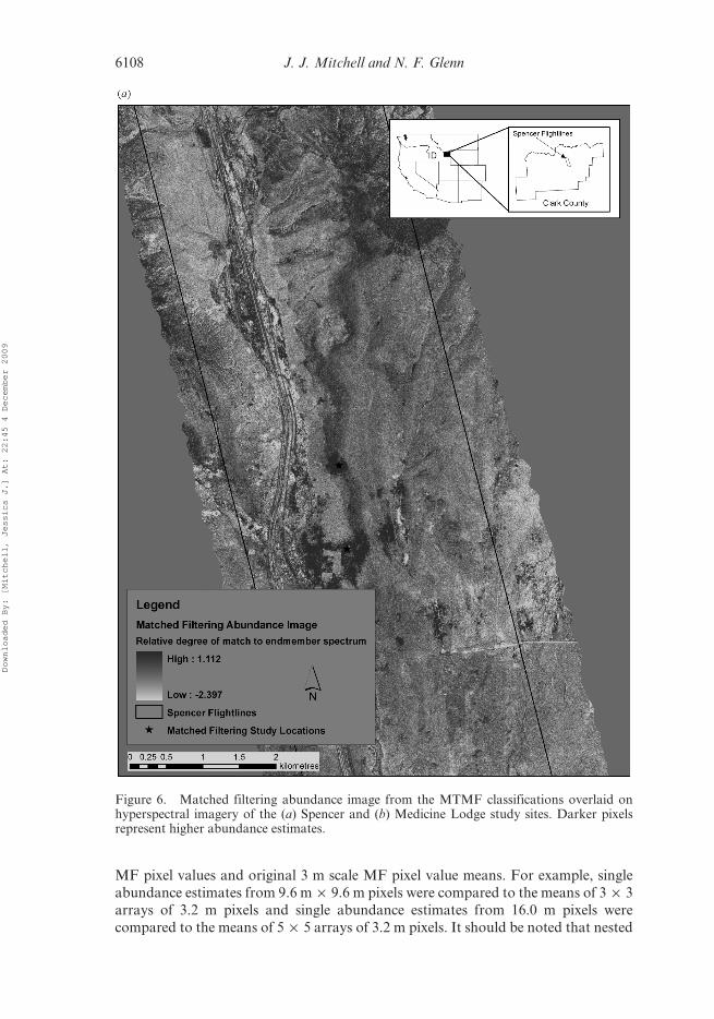
maps generated for Spencer and Medicine Lodge were used to identify three locationsat each study site known to contain large (greater than a 16 m · 16 m pixel), uniform

infestations of leafy spurge. These locations correspond to plots 6 and 10 in Spencer

(see MF study locations in figure 6(a)) and plots 54, 75 and 85 in Medicine Lodge

(see MF study locations in figure 6(b)). Once these locations were identified, the

Spencer and Medicine Lodge reflectance mosaics were spatially resized by factors of

three and five times the original pixel resolution. The pixels were resized using a

square-wave pixel aggregation approach whereby pixels that contribute to the output

pixel are spectrally averaged (nine contributing pixels for the 9 m scale imagery and25 contributing pixels for the 16 m scale imagery). MTMF classifications were also

applied to these resampled mosaics using endmembers spectrally similar to, and in the

geographic vicinity of, the original classification endmembers. These MTMF classi-

fications produced four additional MF images: two MF images of the Spencer site at

three and five times the original spatial resolution (9.6 m and 16.0 m pixels), and two

MF images of the Medicine Lodge site at three and five times the original spatial

resolution (9.9 m and 16.5 m pixels).

3.4 MF score analysis

Linear regression analysis was used to quantify the relationship between ocular

canopy cover estimates and MF abundance estimates of leafy spurge in Spencer and

Medicine Lodge at the original 3 m pixel scale and at pixel aggregated 9 m and 16 m

scales. Linear regressions at all scales used a mean MF score calculated from both the

pixel containing the centre of the circular field plot (168.25 m2) and the nine surround-

ing MF pixels. To test whether linear regression was appropriate to use for the dataanalysis, modality was assessed with histograms, homoscedasticity was investigated

by plotting residuals versus predicted values and qualitatively assessing the regression

plots, and error normality was tested using the Shapiro–Wilk test. A non-parametric

test, the Mann–Kendall, was also used to test for the presence of upward trends in MF

scores across increasing ground cover intervals. The Mann–Kendall is a rank-based

trend test that is applied to vector data, often time series (Mann 1945). For the

purposes of this dataset, ground cover was treated as time and MF scores were treated

as a series.To explore the relationship between spatial scaling and MF score behaviour,

sampling units with dimensions of one, three and five times the original pixel sizes

(3.3 m in Spencer and 3.2 m in Medicine Lodge) were located within six locations

containing large, uniform infestations of leafy spurge (three in Spencer and three in

Medicine Lodge). The large, uniform infestations contained field plots and were

considered necessary to control for the influence of mixing from non-target reflec-

tance and scaling issues; that is, varying ratios of sample support size (field sample size

of 168.25 m2) to prediction support size (successively coarser MF score pixel sizes).The sampling units were arranged within selected infestations such that successively

coarser MF pixels fell in a nested arrangement. The nested arrangement was selected

to optimize comparison of original and pixel-aggregated MF values across spatial

scales. At all six locations, comparisons were made between pixel-aggregated



MF pixel values and original 3 m scale MF pixel value means. For example, single

abundance estimates from 9.6 m · 9.6 m pixels were compared to the means of 3 · 3

arrays of 3.2 m pixels and single abundance estimates from 16.0 m pixels were

compared to the means of 5 · 5 arrays of 3.2 m pixels. It should be noted that nested

Figure 6. Matched filtering abundance image from the MTMF classifications overlaid onhyperspectral imagery of the (a) Spencer and (b) Medicine Lodge study sites. Darker pixelsrepresent higher abundance estimates.



pixel arrangements of three overlapping image scales (3, 9 and 16 m) results in nested

sampling units that do not occur continuously throughout a conceptually composite

image. Consequently, while four of the nested sampling units intersected their respec-

tive field plots, a fifth sampling unit was located approximately 3.5 m from a field plot

and a sixth sampling unit was located approximately 7.5 m from a field plot.

Figure 6. (Continued.)



4. Results

Exploratory data analysis indicated a tendency towards bimodality for leafy spurge

cover and MF scores at all scales in both Spencer and Medicine Lodge. However,

when absence samples were excluded, bimodality was not found in the leafy spurge

cover and MF score data. Thus, two datasets were retained for the regression analysis:

one dataset containing both presence and absence samples and one dataset containing

only presence samples. All of the plots of residuals versus predicted values exhibited a

funnel shape, indicative of non-constant variance (plots not shown). Transformations

(including 1/y, gamma, and log) to stabilize variance were unsuccessful. Thus, homo-scedasticity could not be confirmed. The results of the Shapiro–Wilk test (table 1)

indicate a rejection of the null hypothesis that the residuals have a normal distribu-

tion. However, exclusion of the absence samples in the Shapiro–Wilk test did increase

the normality of the residuals at the 3 m scale in Medicine Lodge (table 1).

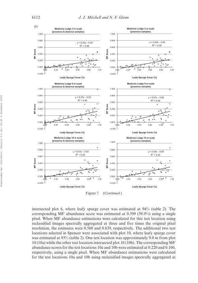
Furthermore, qualitative inspection of the regression plots (figure 7) indicates that

the data behave linearly.

Based on these results, the relationship between ground cover and MF estimates of

leafy spurge was further tested with a non-parametric trend analysis, where slopeestimates near zero indicate no trend. In all cases the Mann–Kendall p-value was

0.000 and the null hypothesis of no significant upward trend in the data was rejected.

The slope estimates from these tests using the Medicine Lodge data were 0.238, 0.324

and 0.248 at the 3, 9 and 16 m scales, respectively. The slope estimates using the

Spencer data were 0.307, 0.251 and 0.224 at the 3, 9 and 16 m scales, respectively.

In the regression plots at the 3 m scale there was strong agreement in Spencer and

fair agreement in Medicine Lodge between field estimates and MF estimates of leafy

spurge abundance (figure 7). A regression analysis that included both presence andabsence reference samples collected at the Spencer site produced an r2 value of 0.63

(n = 51). When absence reference samples were excluded, the agreement still remained

strong (r2 value of 0.63; n = 38). A regression analysis that included both presence and

absence reference samples collected at the Medicine Lodge site produced an r2 value

of 0.46 (n = 55). When absence reference samples were excluded at Medicine Lodge,

the agreement decreased to an r2 value of 0.36 (n = 43). The exclusion of absence

samples consistently yielded slightly lower r2 values at all scales (figure 7). When

Table 1. Shapiro–Wilk normality test results of the residuals from linear regressions of MFabundance estimates versus leafy spurge ground cover at the 95% confidence interval in the

Spencer and Medicine Lodge study sites.

Presence and absence reference samples Presence reference samples

Test statistic p-value Test statistic p-value

Spencer3.2 m 0.897 0.000 0.905 0.0049.6 m 0.818 0.000 0.840 0.00016.0 m 0.763 0.000 0.787 0.000

Medicine Lodge3.3 m 0.951 0.024 0.967 0.240*9.9 m 0.839 0.000 0.874 0.00016.5 m 0.814 0.000 0.849 0.000

*In this case the null hypothesis of normality is accepted.



ocular field estimates of leafy spurge canopy cover were related to MF abundance

scores for resized pixels, agreement declined, with successively larger pixel sizes in

Spencer (9.6 m2, r2 = 0.57; 16 m2, r2 = 0.47; figure 7(a)) and Medicine Lodge (9.6 m2,r2 = 0.46; 16 m2, r2 = 0.42; figure 7(b)). The slopes of all regressions indicate that the

MF scores are underestimating field estimates of leafy spurge cover (considered here

as true abundance). The underestimation is roughly one-third. At both sites, r2 values

were greater than previous results reported by Mundt et al. (2007) and were similar to

results reported by Parker Williams and Hunt (2002).

Analyses of MF scores at different scales also indicated that MF estimates con-

sistently underestimated true abundance (table 2). One test location in Spencer

Spencer 3 m scale (presence & absence samples)

y = 0.32x – 0.02

R2 = 0.64

–0.200

0.000

0.200

0.400

0.600

0.800

1.000

0.00 0.20 0.40 0.60 0.80 1.00

Leafy Spurge Cover (%)

MF

Sco

re

Spencer 3 m scale (presence samples)

y = 0.35x – 0.04

R2 = 0.63

–0.200

0.000

0.200

0.400

0.600

0.800

1.000

0.00 0.20 0.40 0.60 0.80 1.00


MF

Sco

re


y = 0.28x – 0.02

R2 = 0.57

–0.200

0.000

0.200

0.400

0.600

0.800

1.000

0.00 0.20 0.40 0.60 0.80 1.00


MF

Sco

re


y = 0.31 – 0.04

R2 = 0.56

–0.200

0.000

0.200

0.400

0.600

0.800

1.000

0.00 0.20 0.40 0.60 0.80 1.00


MF

Sco

re


y = 0.28x – 0.02

R2 = 0.47

–0.200

0.000

0.200

0.400

0.600

0.800

1.000

0.00 0.20 0.40 0.60 0.80 1.00


MF

Sco

re


y = 0.31x – 0.04

R2 = 0.45

–0.200

0.000

0.200

0.400

0.600

0.800

1.000

0.00 0.20 0.40 0.60 0.80 1.00


MF

Sco

re

(a)

Figure 7. Linear regression plots of MF scores versus leafy spurge cover for the (a) Spencerand (b) Medicine Lodge study sites.



intersected plot 6, where leafy spurge cover was estimated at 94% (table 2). The

corresponding MF abundance score was estimated at 0.599 (59.9%) using a single

pixel. When MF abundance estimations were calculated for this test location using

reclassified images spectrally aggregated at three and five times the original pixelresolution, the estimates were 0.568 and 0.639, respectively. The additional two test

locations selected in Spencer were associated with plot 10, where leafy spurge cover

was estimated at 93% (table 2). One test location was approximately 9.0 m from plot

10 (10a) while the other test location intersected plot 10 (10b). The corresponding MF

abundance scores for the test locations 10a and 10b were estimated at 0.220 and 0.160,

respectively, using a single pixel. When MF abundance estimations were calculated

for the test locations 10a and 10b using reclassified images spectrally aggregated at

Medicine Lodge 3 m scale (presence & absence samples)

y = 0.25x – 0.03

R2 = 0.46

–0.200

0.000

0.200

0.400

0.600

0.800

1.000

0.00 0.20 0.40 0.60 0.80 1.00


MF

Sco

re

Medicine Lodge 3 m scale (presence samples)

y = 0.29x – 0.05

R2 = 0.36

–0.200

0.000

0.200

0.400

0.600

0.800

1.000

0.00 0.20 0.40 0.60 0.80 1.00


MF

Sco

re


y = 0.37x – 0.03

R2 = 0.46

–0.200

0.000

0.200

0.400

0.600

0.800

1.000

0.00 0.20 0.40 0.60 0.80 1.00


MF

Sco

re


y = 0.41x – 0.06

R2 = 0.34

–0.200

0.000

0.200

0.400

0.600

0.800

1.000

0.00 0.20 0.40 0.60 0.80 1.00


MF

Sco

re


y = 0.31x – 0.02

R2 = 0.42

–0.200

0.000

0.200

0.400

0.600

0.800

1.000

0.00 0.20 0.40 0.60 0.80 1.00


MF

Sco

re


y = 0.34x – 0.05

R2 = 0.30

–0.200

0.000

0.200

0.400

0.600

0.800

1.000

0.00 0.20 0.40 0.60 0.80 1.00


MF

Sco

re

(b)

Figure 7. (Continued.)



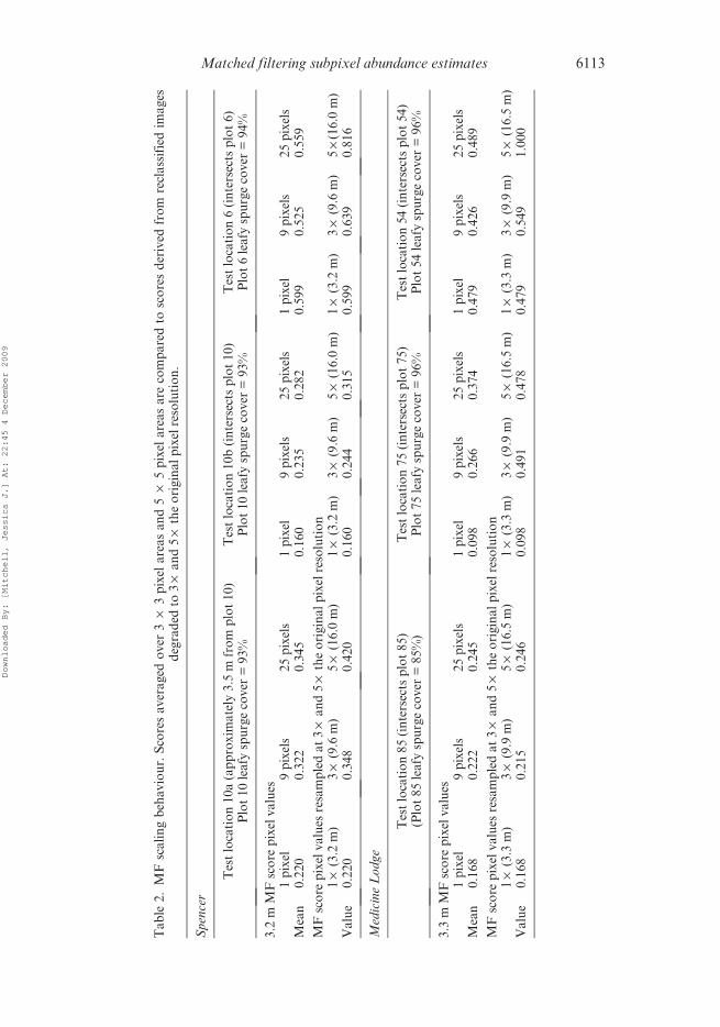
Ta

ble

2.

MF

sca

lin

gb

eha

vio

ur.

Sco

res

av

era

ged

ov

er3

·3

pix

ela

rea

sa

nd

5·

5p

ixel

are

as

are

com

pa

red

tosc

ore

sd

eriv

edfr

om

recl

ass

ifie

dim

ag

esd

egra

ded

to3

·a

nd

5·

the

ori

gin

al

pix

elre

solu

tio

n.

Sp

ence

r

Tes

tlo

cati

on

10

a(a

pp

rox

ima

tely

3.5

mfr

om

plo

t1

0)

Tes

tlo

cati

on

10

b(i

nte

rsec

tsp

lot

10

)T

est

loca

tio

n6

(in

ters

ects

plo

t6

)P

lot

10

lea

fysp

urg

eco

ver

=9

3%

Plo

t1

0le

afy

spu

rge

cov

er=

93

%P

lot

6le

afy

spu

rge

cov

er=

94

%

3.2

mM

Fsc

ore

pix

elv

alu

es1

pix

el9

pix

els

25

pix

els

1p

ixel

9p

ixel

s2

5p

ixel

s1

pix

el9

pix

els

25

pix

els

Mea

n0

.22

00

.32

20

.34

50

.16

00

.23

50

.28

20

.59

90

.52

50

.55

9

MF

sco

rep

ixel

va

lues

resa

mp

led

at

3·

an

d5

·th

eo

rig

ina

lp

ixel

reso

luti

on

1·

(3.2

m)

3·

(9.6

m)

5·

(16

.0m

)1

·(3

.2m

)3

·(9

.6m

)5

·(1

6.0

m)

1·

(3.2

m)

3·

(9.6

m)

5·

(16

.0m

)V

alu

e0

.22

00

.34

80

.42

00

.16

00

.24

40

.31

50

.59

90

.63

90

.81

6

Med

icin

eL

od

ge

Tes

tlo

cati

on

85

(in

ters

ects

plo

t8

5)

Tes

tlo

cati

on

75

(in

ters

ects

plo

t7

5)

Tes

tlo

cati

on

54

(in

ters

ects

plo

t5

4)

(Plo

t8

5le

afy

spu

rge

cov

er=

85

%)

Plo

t7

5le

afy

spu

rge

cov

er=

96

%P

lot

54

lea

fysp

urg

eco

ver

=9

6%

3.3

mM

Fsc

ore

pix

elv

alu

es1

pix

el9

pix

els

25

pix

els

1p

ixel

9p

ixel

s2

5p

ixel

s1

pix

el9

pix

els

25

pix

els

Mea

n0

.16

80

.22

20

.24

50

.09

80

.26

60

.37

40

.47

90

.42

60

.48

9

MF

sco

rep

ixel

va

lues

resa

mp

led

at

3·

an

d5

·th

eo

rig

ina

lp

ixel

reso

luti

on

1·

(3.3

m)

3·

(9.9

m)

5·

(16

.5m

)1

·(3

.3m

)3

·(9

.9m

)5

·(1

6.5

m)

1·

(3.3

m)

3·

(9.9

m)

5·

(16

.5m

)V

alu

e0

.16

80

.21

50

.24

60

.09

80

.49

10

.47

80

.47

90

.54

91

.00

0



three and five times the original pixel resolution, the estimates were 0.348 and 0.244,

respectively, at the 9 m scale and 0.420 and 0.315, respectively, at the 16 m scale. One

test location in Medicine Lodge intersected plot 85, where leafy spurge cover was

estimated at 85% (table 2). The corresponding MF abundance score was estimated at

0.361 using a single pixel. When MF abundance estimations were calculated for thislocation using reclassified images spectrally aggregated at three times and five times

the original pixel size, the 9 m estimate was 0.215 and the 16 m estimate was 0.246.

Two additional test locations in Medicine Lodge intersected plots 75 and 54, where

leafy spurge cover was estimated at 96%. The corresponding MF abundance scores

for the test locations intersecting these plots (75 and 54) were estimated at 0.098 and

0.479, respectively, using a single pixel. When MF abundance estimations were

calculated for test locations in the vicinity of plots 75 and 54 using reclassified images

spectrally aggregated at three and five times the original pixel resolution, the 9 mestimates were 0.491 and 0.549, respectively. The 16 m resized estimates for the test

locations associated with plots 75 and 54 were 0.478 and 1.000, respectively.

Two-sample t-tests were used to statistically compare MF pixel values from the six

study locations at the 3 m and 9 m scale, the 3 m and 16 m scale and the 9 m and 16 m

scale. In all cases there was no statistically significant difference in pixel values

between scales (table 3). Paired t-tests were used to statistically compare averaged

MF pixel scores to aggregated MF pixels scores (table 3). Scores were paired by

location and there was no statistically significant difference between the averaged andthe aggregated scores at both the 9 m and the 16 m scale.

5. Discussion and conclusions

The lack of homoscedasticity from the plots of residuals versus predicted values

indicate that the non-constant variance is a function of leafy spurge cover. Such

non-constant variance could be related to the relative ability to ocularly estimate

leafy spurge cover at different densities (i.e. it may be easier to estimate low and highcover and more difficult to estimate moderate cover). The lack of homoscedasticity

could also be related to inherent heterogenic differences in spatial distribution pat-

terns at various percentage covers. Although the regression plots exhibited linear

characteristics, lack of homoscedasticity and normal error distributions rendered the

resultant r2 values debatable. Mann–Kendall non-parametric trend test results were

Table 3. Student’s t-test results for comparing MF score differences across scales and forcomparing averaged MF pixel scores to aggregated MF pixels scores, paired by location

(95% confidence interval); n = 6.

p-value

Samples3 m and 9 m pixel scale 0.4833 m and 16 m pixel scale 0.2019 m and 16 m pixel scale 0.393

PairsNine MF pixel values averaged over 3 · 3 pixel area vs. a single aggregated MFpixel value at the 9 m scale

0.074

Twenty-five MF pixel values averaged over 5 · 5 pixel area vs. a single aggregatedMF pixel value at the 16 m scale

0.099



consistent with the linear regression results for the presence only data sets in that both

tests provided evidence of a weak to moderate relationship between ground cover and

MF estimates of leafy spurge cover.

Comparative results indicate that the MF score consistently underestimated true

leafy spurge canopy cover. Underestimations are likely to be influenced by fieldmethods for estimating canopy cover, scaling between field estimates and pixel sizes,

limitations inherent to MTMF techniques and by the MTMF classification’s ability to

separate leafy spurge from background spectra. The MF scores were directly related to

ocular cover estimates at the plot scale. While these plot scale estimates were calibrated

and strongly agreed with the average quadrat estimation method (r2 = 0.76), canopy

cover may have been overestimated in the field, thus accounting for the underestima-

tion of MF scores. Although locations of dense, uniform infestations were selected to

reduce the influence of scaling on the relationship between field and MF estimates oftarget abundance, we recognize that the scale of the field plots of leafy spurge cover do

not match the original and resized pixel scales. Specifically, the field estimates were

not made at each incremental pixel size (9, 81 and 256 m2) but were made over a scale of

168 m2. While all six of the field plots were dense, uniform, and at least 256 m2 in area,

overprediction of leafy spurge could have occurred in the field by assuming percentage

cover was homogeneous across these plots. For example, within plot 85 (85% cover),

mixing of other materials may have occurred nonlinearly across the plot. Similarly, we

assume that the plot scale cover estimations could be extrapolated to the larger infestedareas (at least 256 m2). Furthermore, in the cases of plots 10a and 85, the results may be

biased because of the geographical separation between the field plots and the spatially

aggregated MF scores. While field notes indicate that leafy spurge encompassed areas

where MF scores were calculated, our field plots were not ideally situated for the nested

arrangement. A related factor in mismatching between field and image plots is geor-

eferencing. Based on comparisons to GPS data, the Spencer mosaic had a mean

locational error of 0.813 m and the Medicine Lodge mosaic had a mean locational

error of 3.39 m. We suggest that the 168 m2 circular plot is a good size for estimatingleafy spurge percentage cover at the 3–9 m scale. This suggestion is primarily based on

the strong relationship between MF scores and all abundance measurements at the 3–9

pixel scale (table 1).

This variability or tendency towards underestimation is, in part, inherent to the

MTMF technique because it was developed with the idea of estimating subpixel

abundance by measuring the similarity between spectra from image pixels and a single

‘pure’ training spectrum. In the regression analysis, evidence of linearity and high r2

values suggest that MF is, at minimum, providing relative measures of abundance.However, the range in MF scores near 100% canopy cover is large (approximately

0.020–1.000; see figure 7). In another example, table 2 compares the MF values of 3 m

pixels located in dense infestations near 100%. Ideally, these MF values should all be

close to 1.000 but in fact they range in value from 0.098 to 0.599. The degree of

underestimation most probably depends on subtle spectral variation in leafy spurge

and the amount of spectral contrast between the target and the background. Pixels

relatable to target cover near 100% on the ground will be less than 100% because the

spectra will not perfectly match the training pixel spectrum.We also suspect that the MTMF classifications were mistaking some leafy spurge as

background, thereby underestimating target abundance. For example, low contrast will

be associated with a larger underestimation of the abundance. Continued research in

this area is needed and should explore the extent to which the magnitude of



underestimation is a function of scene content. Although we found it more difficult to

separate target pixels from background pixels during the hyperspectral classification of

leafy spurge at the Spencer site (the overall classification accuracy was 67% for Spencer

and 85% for Medicine Lodge), there was better linear regression agreement at the

Spencer site. Better agreement may be attributed to wider ranges in MF score pixelvalues, which provided better spreads for regression analyses. In both Spencer and

Medicine Lodge, the strongest regression relationships occurred at the 3 m pixel scale.

By contrast, the highest abundance estimates tended to occur at coarser scales, whether

estimates were calculated by averaging pixels or extracting scores from spatially

aggregated images. Mann–Kendall slope estimate results indicated the strongest trend

occurred at the 3 m scale in Spencer, but at the 9 m scale in Medicine Lodge. Overall, our

hypothesis that the relationship between MF score and ground cover estimates would

increase as noise is averaged out over coarser spatial resolutions cannot be completelydismissed given inconclusive statistical results and the fact that the highest MF scores

consistently occurred at the 16 m scale for the six high-cover test locations (table 2).

It is difficult to isolate linear MF behaviour from nonlinear MF behaviour because

the distribution of MF scores within an image has a mean of zero and is normalized to

the range of target spectra. In general, if an attribute behaves linearly, then as the

support size increases the mean will remain the same while variance decreases and the

symmetry of the distribution increases (Isaaks and Srivastava 1989). The implication

is that adjustment factors can be calculated to integrate linear attribute data with datacollected at different spatial resolutions. While we cannot directly test MF score

behaviour in such a manner, significance testing across scales and between pixel-

aggregated and pixel-averaged MF estimates suggests there is a linear component to

the MF estimation at the six test locations. Nonlinear mixing is likely to have a greater

influence on MF estimations in other, less ideal environments. Unfortunately, quan-

tifying nonlinearity or even verifying its presence is not a simple process for experi-

mental field data such as ours. Additional studies using simulated laboratory data

would be better suited for determining the extent to which the MF score is a compositemeasurement that exhibits nonlinear scaling behaviour.

Coincidently, it may not be appropriate to relate MF abundance estimates to

vegetation abundance estimates. Unconstrained linear spectral mixture analysis meth-

ods do not necessarily reflect true material abundance fractions and should be inter-

preted for detection, discrimination and classification, not quantification (Heinz and

Chang 2001). Therefore, MF, as a mathematically unconstrained linear spectral

mixture analysis method, generates scores that should only be interpreted as the like-

lihood that a target is contained within a given pixel. While the MTMF classificationtechnique may perform well at detecting the presence of a material, it may not be

equally appropriate for estimating the abundance of materials. Future research should

focus on the use of constrained linear spectral analysis methods to remotely estimate

vegetation abundance (e.g. fully constrained least squares, Heinz and Chang 2001).

Furthermore, because robust ground reference datasets of canopy cover are timely and

costly (e.g. in this study, the number of replicates (n = 6) for testing the resized pixels

versus averaging pixels was not sufficient for definitive conclusions), it would be more

efficient to first test candidate methods under simulated conditions where knownfractions of materials are mixed prior to analysis. When testing a candidate method

in the field, we recommend selecting a demonstration site with a large number of

widespread, uniform infestations and a field sample design where the scale at which

cover is estimated in the field directly corresponds to the scale of resized pixels.



Acknowledgements

We thank the anonymous reviewers who helped to strengthen the merit of this paper.

This research was funded by USDA Natural Resources Conservation Service

Conservation Innovation Grant No. 68-0211-6-124, Pacific Northwest Regional

Collaboratory, as part of a Pacific Northwest National Laboratory project fundedby NASA through Grant No. AGRNNX06AD43G, and NOAA OAR ESRL/

Physical Sciences Division (PSD) Grant No. NA04OAR4600161. Field data collec-

tion was made possible through the generous advice and assistance of Jeffrey

Pettingill and staff at Bonneville County Weed and Pest Control, Shane Jacobson

(US Forest Service, Dubois, Idaho), Keith Bramwell (Continental Divide

Cooperative Weed Management Area), and Tom Stohlgren (USGS Fort Collins

Science Center).

ReferencesANDERSON, G.L., PROSSER, C.W., HAGGER, S. and FOSTER, B., 1999, Change detection of leafy

spurge infestations using aerial photography and geographic information systems. In

Proceedings of the 17th Annual Biennial Workshop on Color Aerial Photography and

Videography in Natural Resource Assessment, 5–7 May 1999, Reno, Nevada (Bethesda,

MD: American Society for Photogrammetry and Remote Sensing).

ASNER, G.P. and LOBELL, D.B., 2000, A biogeophysical approach for automated SWIR unmix-

ing of soils and vegetation. Remote Sensing of Environment, 74, pp. 99–112.

ASPINALL, R.J., MARCUS, W.A. and BOARDMAN, J.W., 2002, Considerations in collecting,

processing, and analyzing high spatial resolution hyperspectral data for environmental

investigations. Journal of Geographical Systems, 4, pp. 15–29.

BATESON, A., ASNER, G.P. and WESSMAN, C.A., 2000, Endmember bundles: a new approach to

incorporating endmember variability into spectral mixture analysis. IEEE Transactions

on Geoscience and Remote Sensing, 38, pp. 1083–1094.

BIRDSALL, J.L., QUIMBY, P.C., SVEJCAR, T. and SOWELL, B., 1995, Image analysis to determine

vegetative cover of leafy spurge. In Proceedings of the 1995 Leafy Spurge Symposium,

Fargo, North Dakota (Sydney, Montana: Team Leafy Spurge), pp. 12–14.

BOARDMAN, J.W., 1998, Leveraging the high dimensionality of AVIRIS data for improved sub-

pixel target unmixing and rejection of false positives: mixture tuned matched filtering.

In Proceedings of the 5th JPL Geoscience Workshop, R.O. Green (Ed.) (Pasadena,

California: NASA Jet Propulsion Laboratory), pp. 55–56.

BONHAM, C.D., 1989, Measurements of Terrestrial Vegetation (New York: John Wiley & Sons).

BOOTH, B.D., MURPHY, S.D. and SWANTON, C.J., 2003, Weed Ecology in Natural and

Agricultural Ecosystems (Cambridge: CABI Publishing).

BOREL, C.C. and GERSTL, S.A.W., 1994, Nonlinear spectral mixing models for vegetative and

soil surfaces. Remote Sensing of Environment, 47, pp. 403–416.

CHANG, C.-I., 2003, Hyperspectral Imaging: Techniques for Spectral Detection and Classification

(New York: Kluwer Academic/Plenum).

DAUBENMIRE, R.F., 1959, A canopy-coverage method. Northwest Science, 33, pp. 43–64.

DEHAAN, R., LOUIS, J., WILSON, A., HALL, A. and RUMBACHS, R., 2007, Discrimination of

blackberry (Rubus fruticosus sp. agg.) using hyperspectral imagery in Kosciuszko

National Park, NSW, Australia. ISPRS Journal of Photogrammetry and Remote

Sensing, 62, pp. 13–24.

DETHIER, M.N., GRAHAM, E.S., COHEN, S. and TEAR, L.M., 1993, Visual versus random-point

percent cover estimations: ‘objective’ is not always better. Marine Ecology Progress

Series, 96, pp. 93–100.

DUDEK, K.B., ROOT, R.R., KOKALY, R.F. and ANDERSON, G.L., 2004, Increased spatial and

temporal consistency of leafy spurge maps from multidate AVIRIS imagery: a hybrid

linear spectral mixture analysis/mixture-tuned matched filtering approach. In



Proceedings of the Thirteenth JPL Airborne Earth Science Workshop. (Pasadena, CA:

NASA Jet Propulsion Laboratory).

EVERITT, J.H., ANDERSON, G.L., ESCOBAR, D.E., DAVIS, M.R., SPENCER, N.R. and ANDRASCIK,

R.J., 1995, Use of remote sensing for detecting and mapping leafy spurge (Euphorbia

esula). Weed Technology, 9, pp. 599–609.

FLOYD, D.A. and ANDERSON, J.E., 1982, A new point interception frame for estimating cover of

vegetation. Vegetatio, 50, pp. 185–186.

GLENN, N.F., MUNDT, J.T., WEBER, K.T., PRATHER, T.S., LASS, L.W. and PETTINGILL, J., 2005,

Hyperspectral data processing for repeat detection of small infestations of leafy spurge.

Remote Sensing of Environment, 95, pp. 399–412.

GREEN, A.A., BERMAN, M., SWITZER, P. and CRAIG, M.D., 1988, A transformation for ordering

multispectral data in terms of image quality with implications for noise removal. IEEE

Transactions on Geoscience and Remote Sensing, 26, pp. 65–74.

HARSAYNI, J.C. and CHANG, C.-I., 1994, Hyperspectral image classification and dimensionality

reduction: an orthogonal subspace projection approach. IEEE Transactions on

Geoscience and Remote Sensing, 32, pp. 779–784.

HEINZ, D.C. and CHANG, C.-I., 2001, Fully constrained least squares linear spectral mixture

analysis method for material quantification in hyperspectral imagery. IEEE

Transactions on Geoscience and Remote Sensing, 39, pp. 529–545.

HUNT, R.E., MCMURTREY, J.E., PARKER WILLIAMS, A.E. and CORP, L.A., 2004, Spectral

characteristics of leafy spurge (Euphorbia esula) leaves and flower bracts. Weed

Science, 52, pp. 492–497.

ISAAKS, E.H. and SRIVASTAVA, R.M., 1989, An Introduction to Applied Geostatistics (Oxford:

Oxford University Press).

JOHNSON, D.E., 1999, Surveying, mapping, and monitoring noxious weeds on rangelands. In

Biology and Management of Noxious Rangeland Weeds, R.L. Shelley and J.K. Petroff

(Eds), pp. 19–35 (Corvallis: Oregon State University Press).

KESHAVA, N. and MUSTARD, J.F., 2002, Spectral unmixing. IEEE Signal Processing, 19,

pp. 44–57.

KRUSE, F.A., 2003, Preliminary results: hyperspectral maps of coral reef systems using EO-1

Hyperion, Buck Island, U.S. Virgin Islands. In Proceedings of the Twelfth JPL Airborne

Geoscience Workshop. (Pasadena, CA: NASA Jet Propulsion Laboratory), pp. 157–173.

KRUSE, F.A., BOARDMAN, J.W., LEFTKOFF, A.B., YOUNG, J.M. and KIEREIN-YOUNG, K.S., 2000,

HyMap: an Australian hyperspectral sensor solving global problems – results from

the USA HyMap data acquisitions. In Proceedings of the Tenth Australian Remote

Sensing and Photogrammetry Conference, Adelaide, Australia. Casual Productions

(CD-ROM). Available online at: http://www.hyvista.com/wordpresshvc/wp-content/

uploads/2008/08/10arspc_hymap.pdf (accessed 27 July 2009).

MANN, H.B., 1945, Nonparametric tests against trend. Econometrica, 13, pp. 245–259.

MARKHAM, B.L. and TOWNSEND, R.G., 1981, Land cover classification accuracy as a function of

sensor spatial resolution. In Proceedings of the 15th International Remote Sensing of the

Environment (Ann Arbor, Michigan: University of Michigan Press), pp. 1075–1090.

MEESE, R.J. and TOMICH, P.A., 1992, Dots on the rocks: a comparison of percent cover

estimation methods. Journal of Experimental Marine Biology and Ecology, 165,

pp. 59–63.

MUNDT, J.T., STREUTKER, D.R. and GLENN, N.F., 2007, Partial unmixing of hyperspectral imagery:

theory and methods. In Proceedings of the American Society of Photogrammetry and

Remote Sensing, Tampa, Florida. (Bethesda, Maryland: American Society of

Photogrammetry and Remote Sensing), pp. 46–57.

OKIN, G.S., ROBERTS, D.A., MURRAY, B. and OKIN, W.J., 2001, Practical limits on hyperspectral

vegetation discrimination in arid and semiarid environments. Remote Sensing of

Environment, 77, pp. 212–215.



http://www.hyvista.com/wordpresshvc/wp-content/uploads/2008/08/10arspc_hymap.pdf

http://www.hyvista.com/wordpresshvc/wp-content/uploads/2008/08/10arspc_hymap.pdf

O’NEILL, M., USTIN, S.L., HAGER, S. and ROOT, R., 2000, Mapping the distribution of leafy

spurge at Theodore Roosevelt National Park using AVIRIS. In Proceedings of the

Ninth JPL Airborne Earth Science Workshop, R.D. Green (Ed.) (Pasadena, California:

NASA Jet Propulsion Laboratory).

PARKER WILLIAMS, A.E. and HUNT, E.R., 2002, Estimation of leafy spurge cover from hyper-

spectral imagery using mixture tuned matched filtering. Remote Sensing of


PARKER WILLIAMS, A.E. and HUNT, E.R., 2004, Accuracy assessment for detection of leafy

spurge with hyperspectral imagery. Journal of Range Management, 57, pp. 106–112.

RAY, T.W. and MURRAY, B.C., 1996, Nonlinear spectral mixing in desert vegetation. Remote

Sensing of Environment, 55, pp. 59–64.

ROBERTS, D.A., SMITH, M.O. and ADAMS, J.B., 1993, Green vegetation, non-photosynthetic

vegetation, and soils in AVIRIS data. Remote Sensing of Environment, 44, pp. 255–269.

ROBICHAUD, P., LEWIS, S., LAES, D., HUDAK, A., KOKALY, R. and ZAMUDIO, J., 2007, Postfire soil

burn severity mapping with hyperspectral image unmixing. Remote Sensing of


SETTLE, J.J. and DRAKE, N.A., 1993, Linear mixing and the estimation of ground cover

proportions. International Journal of Remote Sensing, 14, pp. 1159–1177.

STOHLGREN, T.J., BARNETT, D.T. and CROSIER, C.S., 2005, Beyond NAWMA – The North American

Weed Management Association Standards. Available online at: http://www.nawma.org/

documents/Mapping%20Standards/BEYOND%20NAWMA%20STANDARDS.pdf

(accessed 27 July 2006).

WOODCOCK, C.E. and STRAHLER, A.H., 1987, The factor of scale in remote sensing. Remote

Sensing of Environment, 21, pp. 311–332.



http://www.nawma.org/documents/Mapping%20Standards/BEYOND%20NAWMA%20STANDARDS.pdf

http://www.nawma.org/documents/Mapping%20Standards/BEYOND%20NAWMA%20STANDARDS.pdf

Subpixel abundance estimates in mixture-tuned matched filtering ...

Documents

Transcript of Subpixel abundance estimates in mixture-tuned matched filtering ...