Predictive Power of Cohort-based Revenue Projection Method

Quant Research Note

ThePredictivePowerofCohort-BasedRevenueProjectionMethod

A Comparison of Revenue Projection Methods June 2021

Hum Capital | 530 7th Ave., Suite 405, New York, NY 10018 | humcapital.com

530 7th ave., suite 405, new york, ny 10018 2

humcapital.com

Summary. At Hum Capital, we leverage big data in order to draw the most accurate financial picture of companies. A crucial element of this picture is the projection of future revenues, given a company’s investment plan. Granular information on each customer transaction allows the Intelligent Capital Market (ICM) to forecast a company’s future revenues more accurately. Cohort-based predictive power can be compared to other common revenue forecast methods, showing in general better performances for private companies on ICM.

TableofContents1. Introduction ..................................................................................................................................................... 3

2. Cohort-Based Revenue Projection ................................................................................................................... 4

3. Cross Sectional Evaluation ............................................................................................................................... 6

Method ............................................................................................................................................................. 6

Data .................................................................................................................................................................. 6

Performance Metrics ........................................................................................................................................ 6

4. Results .............................................................................................................................................................. 7

Summary Statistics ........................................................................................................................................... 7

Easy to Predict and Hard to Predict ................................................................................................................. 8

5. Discussions ..................................................................................................................................................... 10


humcapital.com

1.IntroductionIn startup finance, cash is king. An accurate understanding of how much revenue a company generates, and the rate at which revenue grows, is crucial for modeling its cash balance over time. Yet forecasting revenues for a company is a delicate problem. Virtually, there is an infinite number of assumptions that can be made, which can lead to a very broad range of possible outcomes for a prediction. There is nevertheless a well-defined framework to measure how accurate a prediction method is: we can validate the prediction on a test set (last year’s revenue) and see how far from reality the prediction was.

In more detail, the procedure is the following

1. Split the data into a training (in-sample) set and a test (out-of-sample) set. 2. Use the training set to make a prediction on future revenues, disregarding any information in the test set. 3. Compare the predicted revenues against the test (actual) revenues, given a measure of distance between

the two.

Since steps 1 and 3 are independent of assumptions used to make a prediction, we focus on step 2 in this study. The Corporate Finance Institute lists the following as the top three methods used to forecast revenues:

• Constant Growth. Start with the last historical value and assume a constant growth rate, corresponding to the average historical growth rate. • Moving Average. Consider a rolling window of 5 months and use the average to predict the sixth month. • Linear Regression. Perform a linear regression of the revenue income statement line with the sales and marketing investments income statement line. Use the actual investments in the test set as the investment plan to predict revenues.


humcapital.com

For comparison, we also add to the list, Prophet1, a popular general-purpose, time series forecasting tool as the baseline model. This uses a decomposable time series model to handle common features of business time series, such as trend, seasonality, and holidays, and estimates the parameters using posterior inference.

These four methods assume that an income statement, typically with monthly frequency, represents the entirety of our data set. At Hum, however, we are able to process each individual transaction that a company has had with their customers. This additional information allows us to draw a clearer picture of the company’s financials, and specifically gain accuracy and robustness in predicting revenues.

In this empirical study, we show even a simple median Cohort-Based design performs consistently better than others in cases that are harder to predict, while it performs on par with other methods in easier to predict cases. (Definitions for “easy” and “hard to predict” are provided in Section 4.) We think that a cohort-based approach may be adopted by investors since it exhibits more robust performance and introduces lower downside risks.

2.Cohort-BasedRevenueProjectionThe main source of data for a cohort-based method is customer transactions, or customer tapes, which allows us to define customer cohorts. A cohort is a group of customers that share a common feature. In our case, we say that two customers belong to the same cohort if their first transaction with the company was made in the same month.

Since sales and marketing investment drives customer growth, which in turn generates new revenues, we can model how many new customers the company will acquire based on their investment plan. Specifically, the cohort-based model predicts both the future behavior of existing cohorts and revenues from new cohorts.

Let us define a company’s total revenue as R(t), sales and marketing investments as I(t), where t is a monthly period. Let us also define the revenue from cohort tc at time t as r(t;tc). Now, the total revenue at month t is by construction equal to the sum of the revenue from all cohorts at time t:

1 Details about the module Prophet, see https://facebook.github.io/prophet.


humcapital.com

Below are the steps for the Median Cohort-Based Projection method:

1. Compute each cohort’s revenue as a function of the number of months elapsed since the cohort started: ∆t=t−tc.

2. Normalize each cohort revenue curve dividing by the revenue from the initial month: rʹ(tc,t)=r(tc,t)/r(tc,tc). 3. Compute the median across all cohorts of the normalized revenue retention curve:

This median curve will be a function of the number of months elapsed since the cohort started. In words, rmedian(0) represents the median across all cohorts of the normalized revenue in the month when the cohort is acquired, rmedian(1) represents the median across all cohorts of the normalized revenue in the first month after the cohort is acquired, and so on.

4. For each existing cohort, fill in future values with the median normalized revenue retention curve, multiplied by the initial revenue2 . This enables us to project the revenues from the existing cohorts.

As for new cohorts, assuming that sales and marketing investment correlates to acquiring new customers, we regress investments versus cohort revenues at the time the cohort is acquired (∆t=0). We use the outcome of this linear regression as the new cohorts’ initial revenues, to be then multiplied by the median normalized revenue curve.

2 For example, let us assume the last historical month is t=T and we want to project revenues from the cohort that starts at t=T. From that cohort, we

only have r(T,T), as any future revenues are unknown. The initial normalized revenue is then rʹ(T,T)=1. How do we predict the next revenue from this cohort rʹ(T,T+1)? Intuitively, it makes sense that the last cohort will more or less behave like the previous cohorts, so we can fill in the next normalized revenue rʹ(T,T+1)=rmedian(t=1). Likewise, we can fill in all future revenues from this cohort using the median normalized revenue retention curve. Upon multiplying back each value by r(T,T), we obtain the cohort revenue curve for tc=T.


humcapital.com

3.CrossSectionalEvaluationMethod

To recap, the prediction methods we examine in this study are the following:

• Constant Growth: Straight line for revenue growth; • Moving Average: Simple moving average of monthly revenues;. • Regression: Linear regression on investment plans; • Prophet: Simple out-of-shelf model-free prediction as the benchmark; and • Cohort: Median cohort-based method.

Data All models are trained for each company separately, and validated with forward-looking 12-month projections. Note that we do not consider cross sectional structures (e.g., cross-correlation between companies) to improve projections. In addition, since we focus on a 12-months prediction, companies with insufficient training financial data are systematically excluded from the experiment.

Performance Metrics

Model out-of-sample forecasting performances are measured by the following metrics, where A and F are the actual and forecasted revenues at period t, respectively, and T is the length of the out-of-sample periods:

• Mean Absolute Percentage Errors (MAPE):

• Symmetric Mean Absolute Percentage Errors (SMAPE):

• Root Mean Square Errors (RMSE):


humcapital.com

MAPE is a commonly used measure to determine how accurate a forecasting system is. MAPE is calculated as the absolute error between the actual and forecasted revenues, divided by actual revenues, averaged across all time periods. In practice, this performance measure works best when there are no extremes or zeroes in the data. MAPE puts a heavier penalty on negative errors and favors models that under-forecast rather than over-forecast. This is caused by the fact that the percentage error cannot exceed 100% for forecasts that are too low, while there is no upper limit for the forecasts which are too high.

SMAPE is an adjusted version of MAPE, where instead of dividing absolute errors by the actual revenues. SMAPE divides by the mean between the actual and forecasted revenue for each time period. This resolves the situations where actual values are close to 0, and limits SMAPE values to never be greater than 200%, thus fixing the asymmetric issue presented by the MAPE calculation.

RMSE is another frequently used measure, calculated as the square root of the quadratic mean of the differences. RMSE gives a relatively higher weight to larger errors and is most useful when large errors are particularly undesirable.

While there are other potential performance measures, we choose these three as they are quite commonly used and straightforward to understand. In addition, we focus on MAPE in this study. Due to its heavier penalty for overestimation, MAPE will favor models that under-forecast, and from a credit investor perspective, this allows us to be more considerate of downside risks.

4.ResultsSummary Statistics

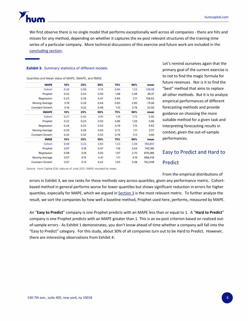
We estimate median returns on investment by month after customer acquisition date for each customer cohort for all companies on ICM, using transaction-level data available from the live feed of customer tapes. These estimated returns, indicative of fundamental business characteristics, are called the return on investment functions (ROIFs, more details see Section 2). We then use these ROIFs to project future revenues based on companies’ investment plans (proxied by realized investments) and compare projected revenues against the actual revenues. We fit models using four other common forecasting methods described in Section 1 based on the same in-sample data set and finally compare the performance metrics of all methods defined in Section 3. The summary statistics are listed in Exhibit 3.


humcapital.com

We first observe there is no single model that performs exceptionally well across all companies - there are hits and misses for any method, depending on whether it captures the ex-post relevant structures of the training time series of a particular company. More technical discussions of this exercise and future work are included in the concluding section.

Let’s remind ourselves again that the primary goal of the current exercise is to not to find the magic formula for future revenues. Nor is it to find the “best” method that aims to replace all other methods. But it is to analyze empirical performances of different forecasting methods and provide guidance on choosing the more suitable method for a given task and interpreting forecasting results in context, given the out-of-sample performances.

Easy to Predict and Hard to

Predict

From the empirical distributions of errors in Exhibit 3, we see ranks for these methods vary across quantiles, given any performance metric. Cohort-based method in general performs worse for lower quantiles but shows significant reduction in errors for higher quantiles, especially for MAPE, which we argued in Section 3 is the most relevant metric. To further analyze the result, we sort the companies by how well a baseline method, Prophet used here, performs, measured by MAPE.

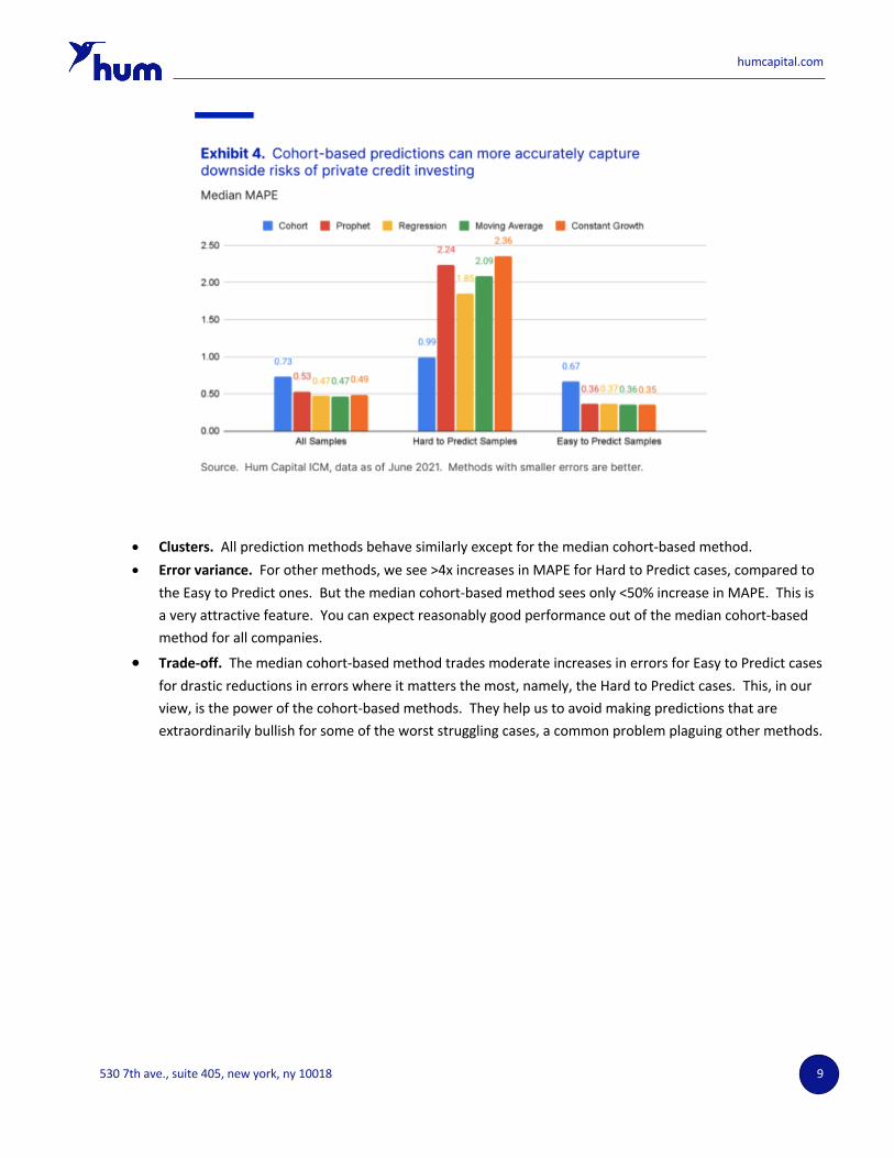
An “Easy to Predict” company is one Prophet predicts with an MAPE less than or equal to 1. A “Hard to Predict” company is one Prophet predicts with an MAPE greater than 1. This is an ex-post criterion based on realized out-of-sample errors - As Exhibit 1 demonstrates, you don’t know ahead of time whether a company will fall into the “Easy to Predict” category. For this study, about 30% of all companies turn out to be Hard to Predict. However, there are interesting observations from Exhibit 4:


humcapital.com

• Clusters. All prediction methods behave similarly except for the median cohort-based method. • Error variance. For other methods, we see >4x increases in MAPE for Hard to Predict cases, compared to

the Easy to Predict ones. But the median cohort-based method sees only <50% increase in MAPE. This is a very attractive feature. You can expect reasonably good performance out of the median cohort-based method for all companies.

• Trade-off. The median cohort-based method trades moderate increases in errors for Easy to Predict cases for drastic reductions in errors where it matters the most, namely, the Hard to Predict cases. This, in our view, is the power of the cohort-based methods. They help us to avoid making predictions that are extraordinarily bullish for some of the worst struggling cases, a common problem plaguing other methods.


humcapital.com

Another way to look at this result is to study the makeup of methods that are highest ranked, i.e., lowest errors, for various samples. We observe from Exhibit 5:

• “Most accurate.” If you

can only use one method out of these methods, pick Cohort. The median cohort-based method is the one that gives you the best results for more companies. This is consistent for all samples, Easy to Predict samples, and Hard to Predict samples.

• “Most reliable.” For Easy to Predict samples, the median cohort-based method performs in line with regressions and moving averages, with Prophet least likely to beat other methods. For Hard to Predict samples, quite remarkably, the median cohort-based method ranks top for 70% of the companies. Prophet is almost certainly to be the worst, with 0% as the top ranked method.

5.DiscussionsWe present an empirical comparison of prediction performance of common time series methods, against a cohort-based method, which uses transaction-level data on Hum Capital’s ICM platform. We test out these methods for all companies on ICM and find a cohort-based method, even in the most naive implementation using median return on investment for each cohort, can provide significant and consistent out of sample improvements for revenue projections against other methods.

The Quant Team at Hum recognizes several key weaknesses of the current study and are working to continuously improve revenue projection methods as well as other quantitative investment research in the private market using transaction-level data feeds on ICM and other alternative data sets. Here are a few key dimensions we plan to improve current work:

• Sample size. Compared to finance research in the public market, our sample sizes, both longitudinal and cross-sectional, are quite limited. This will improve as the ICM platform grows.


humcapital.com

• Macro. This study uses different lookback windows and does not explore cross-sectional structures of companies to improve prediction results. The Quant Team at Hum are actively working on benchmarking private companies on ICM as well as against public companies, this allows us to address macroeconomic effects of different sectors and markets.

• Investment-conditional. The current method uses realized investment instead of ex-ante investment plans and is biased towards cohort-based methods and regressions.

• Median cohort. The current study only uses the median return on investment for each cohort. This is biased against growing companies. This exercise is meant to highlight the potential predictive power of cohort-based methods.

• Sources of truth. This study uses transaction data on ICM as the single source of truth to make the comparisons fair for all methods. Future studies should validate methods against other sources.

530 7th Ave., Suite 405, New York, NY, 10018 humcapital.com

Predictive Power of Cohort-based Revenue Projection Method

Documents

Transcript of Predictive Power of Cohort-based Revenue Projection Method