Prediction of Turbo Compressor Maps using CFDMaster’s thesis in Applied Mechanics

STEPHANIE BERGQVIST

Department of Applied MechanicsDivision of Fluid DynamicsCHALMERS UNIVERSITY OF TECHNOLOGYGothenburg, Sweden 2014Master’s thesis 2014:07

MASTER’S THESIS IN APPLIED MECHANICS

Prediction of Turbo Compressor Maps using CFD

STEPHANIE BERGQVIST

Department of Applied MechanicsDivision of Fluid Dynamics

CHALMERS UNIVERSITY OF TECHNOLOGY

Gothenburg, Sweden 2014

Prediction of Turbo Compressor Maps using CFDSTEPHANIE BERGQVIST

c© STEPHANIE BERGQVIST, 2014

Master’s thesis 2014:07ISSN 1652-8557Department of Applied MechanicsDivision of Fluid DynamicsChalmers University of TechnologySE-412 96 GothenburgSwedenTelephone: +46 (0)31-772 1000

Cover:Streamlines coloured with the magnitude of velocity in a compressor with a rotation rate of 45775 rpm andwith the pressure ratio 1.34.

Chalmers ReproserviceGothenburg, Sweden 2014

Prediction of Turbo Compressor Maps using CFDMaster’s thesis in Applied MechanicsSTEPHANIE BERGQVISTDepartment of Applied MechanicsDivision of Fluid DynamicsChalmers University of Technology

Abstract

Continuous improvements are of great importance in the heavy vehicle industry. Computational fluid dynamics(CFD) can make the developing process easier and can be used for simulations of the compressor in a tur-bocharger. The turbocharger is used in the environment of heavy vehicle engines and is delivered with a turbocompressor map. What is wanted as an outcome from this thesis is a toolchain, as automated as possible, forpredicting turbo compressor maps using CFD.

The used software is STAR-CCM+ and an investigation of parasitic currents was done followed by a creationof a turbo compressor map from simulations. The result from the first part gave information about using arotating reference frame in simulations. The overall results from using CFD to compute a turbo compressormap got close to experimental data available in the project. An automated toolchain was developed containinga similar approach as developing the turbo compressor maps in the project. The realizable k − ε turbulencemodel was used and other turbulence models would be interesting to investigate in the future. Even finermeshes than the used ones could be tested further as well as introducing more truck-like intake systems.

Keywords: CFD, Compressor, Toolchain, STAR-CCM+

i

Preface

This thesis contains a study of simulating compressors by using STAR-CCM+ and the development of atoolchain in Python for creating turbo compressor maps. It has been performed at Scania CV AB in Sodertaljefrom September 2013 to Mars 2014, in collaboration with the Division of Fluid Dynamics at the Department ofApplied Mechanics at Chalmers.

First of all I would like to express my sincere gratitude to my supervisor Dr. Magnus Berglund for all theexpertise and commitment he has contributed during the development of my thesis. I am also very grateful forthe opportunity to do this thesis at Scania. I want to give a special thanks to my examiner Professor LarsDavidson, for being an excellent teacher and taking the responsibility to be my examiner. Last but not least Iwant to thank all my friends and family for always being there when I need them the most.

iii

Contents

Abstract i

Preface iii

Contents v

1 Introduction 11.1 Aim . . . . . . . . . . . . . . . . . . . . . . . . . . . . . . . . . . . . . . . . . . . . . . . . . . . . . 11.2 Research questions . . . . . . . . . . . . . . . . . . . . . . . . . . . . . . . . . . . . . . . . . . . . . 11.3 Delimitations . . . . . . . . . . . . . . . . . . . . . . . . . . . . . . . . . . . . . . . . . . . . . . . . 11.4 Method . . . . . . . . . . . . . . . . . . . . . . . . . . . . . . . . . . . . . . . . . . . . . . . . . . . 11.5 Thesis outline . . . . . . . . . . . . . . . . . . . . . . . . . . . . . . . . . . . . . . . . . . . . . . . . 2

2 Theory 32.1 The airflow through the engine . . . . . . . . . . . . . . . . . . . . . . . . . . . . . . . . . . . . . . 32.2 Turbo Compressor Map . . . . . . . . . . . . . . . . . . . . . . . . . . . . . . . . . . . . . . . . . . 42.3 Navier–Stokes equations . . . . . . . . . . . . . . . . . . . . . . . . . . . . . . . . . . . . . . . . . . 52.4 Reynolds-Averaged Navier–Stokes . . . . . . . . . . . . . . . . . . . . . . . . . . . . . . . . . . . . 52.5 Realizable k − ε turbulence model . . . . . . . . . . . . . . . . . . . . . . . . . . . . . . . . . . . . 62.6 The wall region . . . . . . . . . . . . . . . . . . . . . . . . . . . . . . . . . . . . . . . . . . . . . . . 6

3 Computational studies 93.1 Parasitic currents . . . . . . . . . . . . . . . . . . . . . . . . . . . . . . . . . . . . . . . . . . . . . . 93.1.1 Geometry . . . . . . . . . . . . . . . . . . . . . . . . . . . . . . . . . . . . . . . . . . . . . . . . . 93.1.2 Mesh . . . . . . . . . . . . . . . . . . . . . . . . . . . . . . . . . . . . . . . . . . . . . . . . . . . 103.1.3 Setup . . . . . . . . . . . . . . . . . . . . . . . . . . . . . . . . . . . . . . . . . . . . . . . . . . . 113.1.4 Results . . . . . . . . . . . . . . . . . . . . . . . . . . . . . . . . . . . . . . . . . . . . . . . . . . 113.1.5 Discussion . . . . . . . . . . . . . . . . . . . . . . . . . . . . . . . . . . . . . . . . . . . . . . . . . 153.1.6 Continuing conclusions . . . . . . . . . . . . . . . . . . . . . . . . . . . . . . . . . . . . . . . . . 153.2 Compressor simulations . . . . . . . . . . . . . . . . . . . . . . . . . . . . . . . . . . . . . . . . . . 163.2.1 Geometry . . . . . . . . . . . . . . . . . . . . . . . . . . . . . . . . . . . . . . . . . . . . . . . . . 163.2.2 Mesh . . . . . . . . . . . . . . . . . . . . . . . . . . . . . . . . . . . . . . . . . . . . . . . . . . . 173.2.3 Simulations . . . . . . . . . . . . . . . . . . . . . . . . . . . . . . . . . . . . . . . . . . . . . . . . 183.2.4 Outcome and verification of the results . . . . . . . . . . . . . . . . . . . . . . . . . . . . . . . . 18

4 Toolchain 25

5 Discussion and Conclusions 27

v

1 Introduction

In the heavy vehicle industry there is a continuous development of vehicles and engines with the goal to achievelow pollutant emissions and high efficiency in order to fulfil upcoming legislations and to be competitive. Thisrequires an understanding of how the engine behaves at certain conditions and how all parts of it interact. Thegas exchange process is of great importance when it comes to the efficiency of the engine. A part of this processinvolves the turbocharger.

The behaviour of a turbocharger is mainly tested experimentally and the result is often presented in turbocompressor maps, which contains information of how the compressor will perform at different operatingconditions. These maps are usually obtained from the turbocharger suppliers and might not provide enoughinformation for the company manufacturing the engines. To receive more detailed information in an easier way,Computational Fluid Dynamics (CFD) can be used.

If it is possible to predict more detailed turbo compressor maps and make them readily usable for GT Power itwill be easier to propose design improvements. GT Power is a software which is used for assessing gas exchangeperformance. Another use would be to virtually test (yet) non-existing compressors by combining differentcompressor housings and compressor wheels.

1.1 Aim

The aim of this thesis is to develop a toolchain, as automated as possible, for predicting turbo compressor mapsusing CFD.

1.2 Research questions

There are mainly three questions that are relevant to the research which will help to reach the goal that thisthesis aims for. These research questions are presented below.

• How does the results from the simulations compare to the experimental data in the turbo compressormaps?

• What settings and workflow are preferred for the simulations to get accurate results of the turbo compressormaps?

• Is it possible to predict what happens in the area of surge?

1.3 Delimitations

The investigation will not look at what happens in the surrounding connected to the compressor in an engineinstallation.

1.4 Method

This thesis consists of three main parts and they are done in a specific order as they depend on each other.The compressor is the common factor and the high speeds that appears inside a compressor is considered. Thefirst part involves an investigation of parasitic currents which can appear when using the chosen simulationsoftware STAR-CCM+. The purpose of the second part is to find a method to create turbo compressor mapsand the third and final part has the purpose to develop a toolchain for predicting turbo compressor maps usingPython and STAR-CCM+ with JAVA scripts.

1

1.5 Thesis outline

This report is divided into five chapters. After the introduction follows Chapter 2, the theory chapter, whichfirst shows an overview of where the compressor is situated in the engine and how the air flows through theengine. Then an explanation of a turbo compressor map is done, followed by the theory connected to themechanics of fluids and turbulence modelling.

Followed by this comes Chapter 3 which shows and explains geometries, setups and results for the computationalstudies in this thesis. This chapter is divided into two parts, a parasitic current and a compressor part. A dis-cussion for the first part will be done before continuing to the second part, as the second part depends on the first.

The last part of the project is presented in Chapter 4, where the toolchain developed in the project is shownand explained.

Furthermore, discussion and conclusions can be found in Chapter 5.

2

2 Theory

2.1 The airflow through the engine

The engine needs air for the combustion in the cylinders and the main parts where the air flows through canbe seen in Figure 2.1. The air intake system can be shaped in many different ways, but in all cases there arepressure losses along the way. Manufacturers try to minimize the losses but it can be difficult with all othercomponents situated in the vicinity in the engine. On the way from the air intake to the compressor, the airhas to pass through an air filter which cleans the air from larger particles.

Next, the air flows into the compressor which is increasing the pressure. This also means that the air getswarmer, therefore the air is cooled down in the charge-air cooler before entering the combustion in the cylinders.The air is supposed to be cooled as much as possible to get a higher efficiency of the engine. The exhaust gasesflows into the turbine, which will be the driving component of the compressor. The aftertreatment systemtakes care of the exhaust gases to reduce emissions and the muffler act as the last silencer.

Figure 2.1: Main components for airflow through engine.

Turbocharger

The combination of a turbine and a compressor is called a turbocharger. The purpose of this is to increase theeffect of the engine by supplying more air to the combustion in the cylinders. What drives the turbocharger arethe exhaust gases which makes the turbine wheel spin. A shaft transfers the kinetic energy to the compressorwheel which compresses the air. See an example of a turbocharger geometry in Figure 2.2.

Figure 2.2: Turbocharger. Picture after H. Jaskelainen, M.K. Khair [8].

3

2.2 Turbo Compressor Map

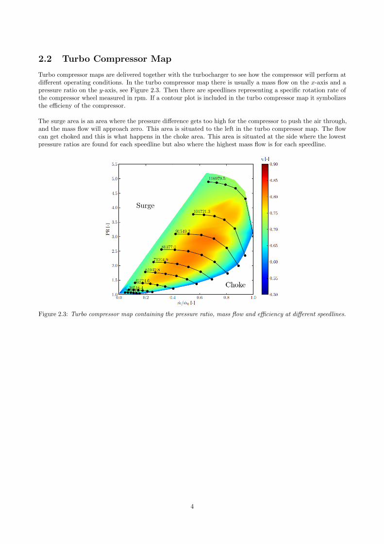
Turbo compressor maps are delivered together with the turbocharger to see how the compressor will perform atdifferent operating conditions. In the turbo compressor map there is usually a mass flow on the x-axis and apressure ratio on the y-axis, see Figure 2.3. Then there are speedlines representing a specific rotation rate ofthe compressor wheel measured in rpm. If a contour plot is included in the turbo compressor map it symbolizesthe efficieny of the compressor.

The surge area is an area where the pressure difference gets too high for the compressor to push the air through,and the mass flow will approach zero. This area is situated to the left in the turbo compressor map. The flowcan get choked and this is what happens in the choke area. This area is situated at the side where the lowestpressure ratios are found for each speedline but also where the highest mass flow is for each speedline.

Figure 2.3: Turbo compressor map containing the pressure ratio, mass flow and efficiency at different speedlines.

4

2.3 Navier–Stokes equations

The governing equations for a fluid flow are usually called the Navier–Stokes equations which are composed bythe combination of the continuity equation and the momentum equation but for a compressible flow the energyequation must also be considered [7] [11]. These equations are composed as follows,

∂ρ

∂t+∂(ρvi)

∂xi= 0 (2.1)

∂(ρvi)

∂t+∂(ρvjvi)

∂xj= − ∂p

∂xi+∂τij∂xj

+ ρfi (2.2)

∂

∂t

[ρ

(e+

1

2vivi

)]+

∂

∂xj

[ρvj

(h+

1

2vivi

)]=

∂

∂xj(viτij) −

∂qj∂xj

(2.3)

where ρ is the density, v is the instantaneous velocity, p is the pressure, f is the body force acting on the fluidparticle, e is the specific internal energy and h = e+ p/ρ is the specific enthalpy. The use of the ideal gas lawgives a relation between the pressure, density and the temperature which is computed as

p = ρRT. (2.4)

The viscous stress tensor τij in a compressible flow, includes a second viscosity, ζ, which is assumed to berelated to the dynamic viscosity µ as

ζ = −2

3µ (2.5)

and the constitutive relation between the stress and strain rate tensors becomes

τij = 2µSij +2

3µSkkδij (2.6)

where δij is the Kronecker delta and the strain rate tensor computed as

Sij =1

2

(∂vi∂xj

+∂vj∂xi

). (2.7)

The heat flux vector qj in Equation (2.3) can be obtained from Fourier’s law [11] giving

qj = −κ ∂T∂xj

(2.8)

with κ as the thermal conductivity.

2.4 Reynolds-Averaged Navier–Stokes

Using Navier–Stokes gives a lot of information and is very time consuming as it requires a very fine resolutionin space and time. Every quantity can be decomposed into a sum of a time-averaged value and a fluctuation as

Φ(xi, t) = Φ(xi) + Φ′(xi, t) (2.9)

where

Φ(xi) = limT→∞

1

T

∫ T

0

Φ(xi, t)dt (2.10)

The use of Equation (2.9) together with the Navier–Stokes equations gives the Reynolds-Averaged Navier–Stokes(RANS) equations. This causes a closure problem which is solved through turbulence modelling. No model isperfect but usually gives a good approximation if the right model for a specific problem is used. As the meanvalues of the flow quantities mainly are of interest in engineering, RANS equations are convenient to use [5] [7].

5

2.5 Realizable k − ε turbulence model

The standard k − ε model is a widely used two-equation model which uses the modelled equations of theturbulent kinetic energy k and turbulent dissipation ε to solve the scalar field of k and ε. Example of quantitieswhich can be computed are a turbulent length scale (LT = k3/2/ε) and a timescale (τ = k/ε) [9]. The modelledequations are developed from the exact equations of k and ε which can be found in Ferziger and Peric, andShih et al. [7] [10]. But this model can also create unphysical values because of the eddy viscosity which getsover-predicted by the standard formulation [10]. Another transport equation for the dissipation is created and anew eddy-viscosity is formulated and its outcome is the realizable k − ε model, proposed by Shih et al. [10] [1].

2.6 The wall region

At the wall and close to it, a lot of things happen and in complex geometries it is difficult to predict thebehaviour. With x1, x2 and x3 as the streamwise, wall-normal and crosswise coordinates, a simple case ofchannel flow will give some general explanation in this section. The setup is given by two plates on either sideand an infinite span in the x3-direction. The wall region is shown up to the centreline in Figure 2.4 and theregion is divided into a couple of regions.

Figure 2.4: Wall region. Picture after Davidson [5].

In the viscous region the flow is dominated by the viscous forces and the wall shear stress is important to havein mind. The calculation of the wall shear stress is done by taking the mean velocity in the first cell by thewall and the x2-value in the centre of the cell:

τw = µ∂v1∂x2

∣∣∣∣w

(2.11)

where the velocity is zero from a no-slip boundary condition at the wall but increases a lot in the beginning,and the velocity gradient in the main flow direction against the x2 axis becomes very large. The velocity profilefor fully developed turbulent flow is shown in Figure 2.5.

To calculate the dimensionless value of x+2 , a friction velocity can be computed as uτ = (τw/ρ)1/2. The equationfor the dimensionless x+2 -value can then be computed as x+2 = x2uτ/ν and y+ = x+2 . A simple geometry of acell near the wall can be seen in Figure 2.6. When doing CFD it is sometimes preferred to have a y+-valuefor the first node in the log-law region to be able to use wall functions. This requires y+ ≥ 30 and will alsomean that the boundary near the wall is not resolved [6]. According to ANSYS the absolute minimum value touse is y+≈ 15 [1]. STAR-CCM+ is not informing about preferred limits and is another software than the oneANSYS develops. The limits from ANSYS is not necessarily the same for STAR-CCM+ and the investigationin Chapter 3 will show that lower values than 15 could be possible to use. If not using wall functions the valueof y+should be less than one.

6

Figure 2.5: Velocity profile for a fullydeveloped turbulent channel flow.

Figure 2.6: Cell adjacent the wallwith its centre position.

The boundary layer for a turbulent flow using a logarithmic scale for y+ can be seen in Figure 2.7. In thesection closest to the wall the velocity profile is well approximated to be linear and v+ = y+. But further awaythe velocity profile is logarithmic and can be estimated as

v+ =1

κln y+ +B. (2.12)

This behaviour is called the law of the wall according to Wilcox [11]. The layer which is not linear norlogarithmic is the buffer region. The two-layer wall treatment together with fine meshes is supposed to resolvethe viscous sublayer in STAR-CCM+ [4].

Figure 2.7: Wall region with a linear and logarithmic law for the boundary layer. Picture after Ferziger andPeric [7].

7

3 Computational studies

This chapter is divided into two parts where the purpose of the first part is to get better understanding of thebehaviour of the simulation software STAR-CCM+ when introducing higher velocities together with a multiplereference frame (MRF) close to a wall. A rotating coordinate system is used for the MRF region as the wheel inthe compressor later on will have this type of setup. The errors and disturbances that are caused by using thissetup together with the chosen simulation software, are called parasitic currents which was investigated in thispart. The resolution and structure of the mesh were tested together with different operating conditions andthe outcome was evaluated. The knowledge gained from this part was applied to the setup of the compressorsimulations. The chosen turbulence model was the realizable k − ε two-layer model as it is commonly used andit was used throughout the whole project.

The second part involved CFD-simulations of a compressor to create a turbo compressor map based on datafrom experimental tests. The geometry was given but an MRF had to be created, which covered the compressorwheel and had an interface between the compressor house and the compressor wheel. The spacing betweenthese two surfaces could be as small as 0.3 mm. With the knowledge gained from the previous part of theproject, the mesh was created. The workflow to create the turbo compressor map was later on applied in thefinal part of the project which is presented in the next chapter.

3.1 Parasitic currents

The simple geometry that was used for the parasitic current part will be presented first, followed by the creationof different meshes and then the setup of different operation conditions. The values of input parameters weretaken from standard values which are commonly used. A presentation of the results is done followed by adiscussion and finally a short conclusion is given which is used in the next main study of the project.

3.1.1 Geometry

A straight pipe was used as the geometry, see Figure 3.1. A MRF was created as a smaller cylindrical regionwith its own rotational coordinate system and can be referred to as a rotating reference frame. This region wassituated in the middle between the inlet and the outlet. The distances between the inlet and outlet to theMRF region are ten times the diameter. This was used so that the flow will become fully developed beforereaching the MRF region. Note the small distance between the smaller and larger cylinder. This gap emulatesthe small gap in the compressor between the house and the wheel. The dimensions were set to D = 0.0757 m,DMRF = 0.0726 m and LMRF = 0.06 m.

Figure 3.1: Geometry of cylinder and MRF region for testing of parasitic currents.

9

Table 3.1: Settings for Parasitic currents.

Mesh Basesize[m]

Relativeminsize[%]

Relativemin sizeMRF[%]

Relativetargetsize[%]

Relativetargetsize MRF[%]

Surfacegrowthrate[-]

Prismlayerthickness[%]

Prismlayerthickness[m]

Prismlayers atinterface

Volumemeshsize[cells]

a 0.001 25 25 500 500 1.2 33.3 N/A No 444 852b 0.001 25 25 500 500 1.2 66.6 N/A No 428 931c 0.001 20 10 500 100 1.1 66.6 N/A No 488 702d 0.001 20 10 500 100 1.1 66.6 N/A Yes 680 208e 0.001 20 N/A 500 N/A 1.1 66.6 N/A N/A 133 254f 0.0006 20 10 500 100 1.1 66.6 N/A No 752 939g 0.0006 20 10 500 100 1.1 66.6 N/A Yes 940 846h 0.0006 20 N/A 500 N/A 1.1 66.6 N/A N/A 410 767i 0.0004 20 10 500 100 1.1 66.6 N/A No 1 508 954j 0.0004 20 10 500 100 1.1 66.6 N/A Yes 1 688 888k 0.0004 20 N/A 500 N/A 1.1 66.6 N/A N/A 1 187 893l 0.0004 20 N/A 500 N/A 1.1 N/A 6.66e-4 N/A 1 184 392m 0.0002 20 10 500 100 1.1 66.6 N/A No 9 687 244n 0.0002 20 10 500 100 1.1 66.6 N/A Yes 9 896 359

3.1.2 Mesh

A polyhedral mesher was used as it is commonly used. Several values of the mesh settings were changed to testdifferent resolutions and properties of the mesh. Prism layers at the interface was tested to see if a MRF witha rotating coordinate system needs a better resolved mesh at the interface to give a better transition whenchanging the relation for the equations between the two reference frames. If the prism layers are necessary orsignificantly better to use, they will have to be included in the compressor simulations and it would increasethe size of the mesh. The MRF was also removed completely to see what impact it had on the simulations. InTable 3.1 all tested meshes are presented with their specified settings. All percentage values are related to thespecified base size.

10

3.1.3 Setup

The inlet was a mass flow inlet and the outlet a pressure outlet, the general settings for the conditions arepresented in Table 3.2 where LT is the turbulent length scale.

Table 3.2: Settings for inlet and outlet condition.

p [Pa] T [K] I [%] LT [m]

Inlet condition 0.0 300 5 0.01Outlet condition 0.0 300 0.1 0.01

The MRF region had a rotating coordinate system which was used in a rotating reference frame. The rotationspeed and the mass flow condition were changed to get different operation conditions (OC). These conditionscan be seen in Table 3.3. The operating conditions were combined with the different meshes.

Table 3.3: Operating conditions for Parasitic currents.

OC Mass flow[kg/s]

Speed MRF[rpm]

1 0.5 N/A2 0.5 03 0.2 50 0004 0.5 90 000

3.1.4 Results

In this section the result of the simulations is shown. All values are taken from a cross section in the middle ofthe geometry. The wall y+-values are investigated as well as a velocity ratio which is computed by the velocityin the y-direction, the spanwise direction, divided by the velocity in the x-direction, the streamwise direction.The velocity ratio should be as small as possible as the streamwise velocity should be much larger than thespanwise velocity, which should be zero in a fully developed flow. The standard deviation is investigated andshould be zero, as the pressure should be constant over the cross section and not have any variation over theplane.

Prism layer at interface or not

There was a question if prism layers were needed at the interface. If they were needed, the amount of cellswould increase and it might be difficult to put prism layers at the MRF interface in the compressor geometry.The results from using prism layers at the interface is presented in Table 3.4 and the results with the sameoperating condition but without prism layers at the interface is presented in Table 3.5.

Table 3.4: Resolution testing result with prism layer at interface.

Mesh OC Wall y+ [-] (vy/vx)max [%] Standard deviation [Pa]

d 4 12.4-14.9 5.7 15.1g 4 12.1-15.0 4.4 12.5j 4 7.3-9.6 6.3 11.0n 4 3.1-4.2 6.3 14.1

When using the coarsest mesh the y+-values gets higher and the velocity ratio and the standard deviation getslower compared to not use a prism at the interface. This indicates that no prism layer is needed. Otherwise theresult is quite similar but slightly better in the standard deviation when using a prism layer. The y+-valuedoes not lie in a optimal region as the preferred minimum value is 15 or below one. Something to notice is that

11

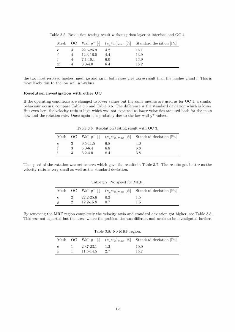
Table 3.5: Resolution testing result without prism layer at interface and OC 4.

Mesh OC Wall y+ [-] (vy/vx)max [%] Standard deviation [Pa]

c 4 22.6-25.9 4.2 15.1f 4 12.3-16.0 4.4 13.9i 4 7.1-10.1 6.0 13.9m 4 3.0-4.0 6.4 15.2

the two most resolved meshes, mesh j,o and i,n in both cases give worse result than the meshes g and f. This ismost likely due to the low wall y+-values.

Resolution investigation with other OC

If the operating conditions are changed to lower values but the same meshes are used as for OC 1, a similarbehaviour occurs, compare Table 3.5 and Table 3.6. The difference is the standard deviation which is lower.But even here the velocity ratio is high which was not expected as lower velocities are used both for the massflow and the rotation rate. Once again it is probably due to the low wall y+-values.

Table 3.6: Resolution testing result with OC 3.

Mesh OC Wall y+ [-] (vy/vx)max [%] Standard deviation [Pa]

c 3 9.5-11.5 6.8 4.0f 3 5.0-6.4 6.8 6.8i 3 3.2-4.0 8.4 3.8

The speed of the rotation was set to zero which gave the results in Table 3.7. The results got better as thevelocity ratio is very small as well as the standard deviation.

Table 3.7: No speed for MRF.

Mesh OC Wall y+ [-] (vy/vx)max [%] Standard deviation [Pa]

c 2 22.2-25.6 0.2 1.5g 2 12.2-15.8 0.7 1.5

By removing the MRF region completely the velocity ratio and standard deviation got higher, see Table 3.8.This was not expected but the areas where the problem lies was different and needs to be investigated further.

Table 3.8: No MRF region.

Mesh OC Wall y+ [-] (vy/vx)max [%] Standard deviation [Pa]

e 1 20.7-23.1 1.2 10.0h 1 11.5-14.5 2.7 15.7

12

Problem areas

The area where the velocity ratio problems occurs when having an MRF region is closest to the interface onthe side closest to the outer cylinder, see Figure 3.2. If removing the MRF region, the problem is moved fromthe interface to the prism layer, see Figure 3.3.

When a larger prism layer is introduced it will involve the wall y+value directly. It is noticable in Figure 3.3that the prism layer cells are very stretched, which decreases the wall y+-value. The results from Table 3.9show that the cases with a larger prism layer has in general better values. Note that even if the wall y+-valuelies around 10 the result is surprisingly good with a low velocity ratio and low standard deviation.

When using a mesh containing an MRF region the result in velocity ratio and standard deviation difference isquite similar even if the wall y+-values is not the same. For the case without any MRF region, the result of thevelocity ratio is significantly different and better when using larger prism layer cells.

Table 3.9: Prism layer size.

Mesh OC Wall y+ [-] (vy/vx)max [%] Standard deviation [Pa]

a 2 10.1-13.2 0.4 2.0b 2 22.0-25.4 0.2 2.1k 1 6.7-8.9 3.6 11.8l 1 21.3-22.6 0.7 9.8

13

Figure 3.2: vy/vx for case with Mesh c and OC 4.

Figure 3.3: vy/vx for case with Mesh e and OC 1.

14

3.1.5 Discussion

The result from using prism layers or not at the interface of the MRF region gave similar result and therefore itis preferred to not use prism layers at the interface. This will reduce the amount of cells. Another positiveoutcome of this is that it will not be necessary to try to create a large amount of cells in the really small gapbetween the compressor wheel and compressor house where the MRF region has its interface. Then the focusof prism layer can be put on other parts of the geometry where it is really needed.

A lower mass flow and a lower rotation rate but the same meshes can give very different results which isprobably due to the velocity gradient in the first node by the wall. Lower difference value of the velocity iscreated in the centre of the nodes but uses the same distance from the wall as before and this will give lowerwall y+-values. This can be good to keep in mind if different speeds are simulated in the same mesh. Usingzero rotation speed gives some errors in the solution but they were significantly small. Therefore the MRFregion itself does not seem to affect the simulation a lot and with y+≈ 10, the result was surprisingly good.But when any speed is involved there are disturbances in the solution to keep in mind and a higher value of thewall y+-value is preferred to use.

Using no MRF region but the same mesh settings, gave high standard deviations and higher velocity ratios.The problem areas were moved from the interface to the prism layers at the large cylinder. The prism layer cellsgot very stretched which is not preferred for CFD simulations, no matter what cells are involved. If the cellswere enlarged in the prism layers, the result got much better which was most likely due to the wall y+-values.

3.1.6 Continuing conclusions

The main conclusion is that the prism layer at the interface is not necessary to use and will not be used for thenext part of the project as it gives similar result as if not using a prism layer. The MRF region itself givessome errors but they are significantly small. When rotational speed is involved, the computational errors areenlarged. The final conclusion is that the prism layers and the wall y+-values matters a great deal and shouldbe considered in the next part.

15

3.2 Compressor simulations

In this part of the report the given geometry will be presented at first followed by how the mesh was structured.The workflow of the simulations is also explained and finally the result from the simulations will be presented.

3.2.1 Geometry

The geometry of the compressor was given and can be seen in Figure 3.4. The compressor wheel is situatedinside the compressor house, and will be encapsulated with a cover which creates the MRF region. Thecompressor wheel and the MRF region can be seen in Figures 3.5 and 3.6.

Two regions existed in total, one stationary region and one rotating region. In the cross section in Figure 3.7 itis possible to see where the intersection between the two regions is located. The zoomed part shows the limitedspace between the blade and house wall with the interface in between.

Figure 3.4: Hollow picture of the compressor.

Figure 3.5: The compressor wheel as a solid. Figure 3.6: The MRF region as a solid.

16

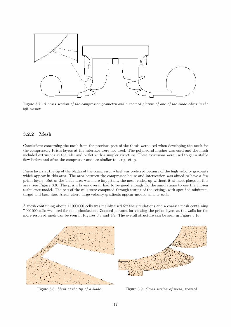
Figure 3.7: A cross section of the compressor geometry and a zoomed picture of one of the blade edges in theleft corner.

3.2.2 Mesh

Conclusions concerning the mesh from the previous part of the thesis were used when developing the mesh forthe compressor. Prism layers at the interface were not used. The polyhedral mesher was used and the meshincluded extrusions at the inlet and outlet with a simpler structure. These extrusions were used to get a stableflow before and after the compressor and are similar to a rig setup.

Prism layers at the tip of the blades of the compressor wheel was preferred because of the high velocity gradientswhich appear in this area. The area between the compressor house and intersection was aimed to have a fewprism layers. But as the blade area was more important, the mesh ended up without it at most places in thisarea, see Figure 3.8. The prism layers overall had to be good enough for the simulations to use the chosenturbulence model. The rest of the cells were computed through testing of the settings with specified minimum,target and base size. Areas where large velocity gradients appear needed smaller cells.

A mesh containing about 11 000 000 cells was mainly used for the simulations and a coarser mesh containing7 000 000 cells was used for some simulations. Zoomed pictures for viewing the prism layers at the walls for themore resolved mesh can be seen in Figures 3.8 and 3.9. The overall structure can be seen in Figure 3.10.

Figure 3.8: Mesh at the tip of a blade. Figure 3.9: Cross section of mesh, zoomed.

17

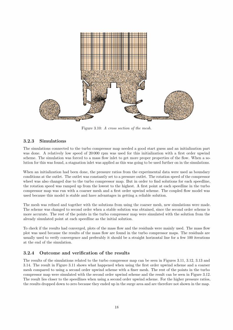
Figure 3.10: A cross section of the mesh.

3.2.3 Simulations

The simulations connected to the turbo compressor map needed a good start guess and an initialization partwas done. A relatively low speed of 20 000 rpm was used for this initialization with a first order upwindscheme. The simulation was forced to a mass flow inlet to get more proper properties of the flow. When a so-lution for this was found, a stagnation inlet was applied as this was going to be used further on in the simulations.

When an initialization had been done, the pressure ratios from the experimental data were used as boundaryconditions at the outlet. The outlet was constantly set to a pressure outlet. The rotation speed of the compressorwheel was also changed due to the turbo compressor map. But in order to find solutions for each speedline,the rotation speed was ramped up from the lowest to the highest. A first point at each speedline in the turbocompressor map was run with a coarser mesh and a first order upwind scheme. The coupled flow model wasused because this model is stable and have advantages in getting a reliable solution.

The mesh was refined and together with the solutions from using the coarser mesh, new simulations were made.The scheme was changed to second order when a stable solution was obtained, since the second order scheme ismore accurate. The rest of the points in the turbo compressor map were simulated with the solution from thealready simulated point at each speedline as the initial solution.

To check if the results had converged, plots of the mass flow and the residuals were mainly used. The mass flowplot was used because the results of the mass flow are found in the turbo compressor maps. The residuals areusually used to verify convergence and preferably it should be a straight horizontal line for a few 100 iterationsat the end of the simulation.

3.2.4 Outcome and verification of the results

The results of the simulations related to the turbo compressor map can be seen in Figures 3.11, 3.12, 3.13 and3.14. The result in Figure 3.11 shows what happened when using the first order upwind scheme and a coarsermesh compared to using a second order upwind scheme with a finer mesh. The rest of the points in the turbocompressor map were simulated with the second order upwind scheme and the result can be seen in Figure 3.12.The result lies closer to the speedlines when using a second order upwind scheme. For the higher pressure ratios,the results dropped down to zero because they ended up in the surge area and are therefore not shown in the map.

18

The overall results from the simulations lies below the given speedline and all simulated points are driven tothe left of their corresponding experimental point. In almost all cases with the second order upwind scheme,the residuals had not fully converged but at least decreased three orders of magnitude.

The turbo compressor maps as contour plots contains the efficiency of the compressor at different operatingconditions as well, see Figures 3.13 and 3.14. The simulated data shows a similar behaviour to the experimentaldata even though the efficiency is not of the same magnitude. There is a red area very close to the surge areain Figure 3.13, but this is a postprocessing error which has nothing to do with the results.

Figure 3.11: A normalized turbo compressor map with pressure ratio against the mass flow, containing theoriginal experimental data. The results from the first order upwind simulations are shown as dots coloured ingreen and the second order upwind simulations are coloured in blue.

Figure 3.12: A normalized turbo compressor map with pressure ratio against the mass flow, containing theoriginal experimental data (black lines) and the results from the simulations (blue lines).

19

0.0 0.2 0.4 0.6 0.8 1.0m/m0 [-]

1.0

1.5

2.0

2.5

3.0

3.5

4.0

4.5

5.0

5.5

PR

[-]

30516.420344.3

81377.0

45774.6

61032.8

91549.2

101721.3

116979.5

71204.9

0.50

0.55

0.60

0.65

0.70

0.75

0.80

0.85

0.90η [-]

Figure 3.13: A normalized contour plot of the turbo compressor map containing the pressure ratio, massflowand efficiency from experimental data.

0.0 0.2 0.4 0.6 0.8 1.0m/m0 [-]

1.0

1.5

2.0

2.5

3.0

3.5

4.0

4.5

5.0

5.5

PR

[-]

81377.0

45774.6

61032.8

91549.2

101721.3

116979.5

71204.9

0.50

0.55

0.60

0.65

0.70

0.75

0.80

0.85

0.90η [-]

Figure 3.14: A normalized contour plot of the turbo compressor map containing the results pressure ratio,massflow and efficiency from the simulated data.

20

The streamlines for a simulated point at 45775 rpm with the pressure ratio 1.34 in the turbo compressor mapcan be seen in Figure 3.15. The flow is stable before it enters the compressor and when it has entered thecompressor and is compressed close to the wheel the speed of the fluid becomes very high. The velocity of theflow after the compressor is slowed down but includes a swirl. A similar behaviour appears for a case with therotation rate 91550 rpm and pressure ratio 2.95, see Figure 3.16. The flow has a higher speed and has evenstronger swirl which is reasonable as the rotation rate is larger. The results for the higher speeds are simi-lar to the lower ones concerning the temperature, pressure and wall y+-distribution, but has higher values overall.

Figure 3.15: Streamlines coloured with the magnitude of velocity for a simulation at 45775 rpm with PR 1.34.

Figure 3.16: Streamlines coloured with the magnitude of velocity for a simulation at 91550 rpm with PR 2.95.

21

The temperature distribution before, through and after the compressor can be seen in Figure 3.17 for a rotationrate of 45775 rpm with the pressure ratio 1.34. The air is compressed which gives an increase in the temperatureafter the compression.

A contour plot of the pressure at the compressor house can be seen in Figure 3.18, where the pressure is high atthe outlet part of the compressor. A contour plot of the pressure distribution at the compressor wheel can beseen in Figure 3.19 and was also used for verifying that the solution is accurate. The highest pressure is foundin the bottom region of the wheel and the lowest at the top and on the top of the blades. The distributionlooks quite symmetric which it should. The result seems reasonable as the purpose of the compressor is tocompress the air.

Figure 3.17: Contour plot of the temperature distribution at the compressor house at 45775 rpm with PR 1.34.

Figure 3.18: Contour plot of the pressure at the compressor house at 45775 rpm with PR 1.34.

22

Figure 3.19: Contour plot of the pressure at the compressor wheel at 45775 rpm with PR 1.34.

Finally the wall y+-values can be seen in Figures 3.20 and 3.21 from the simulations with the rotation rate at45775 rpm and pressure ratio 1.34. There are very low values at the inlet but possibly under the value one.Otherwise most of the result at the house lies in the range from around 20 to around 40. The wall y+-valuesfor the wheel lies in a similar range but are slightly lower. The edge of the blades were adapted to get propervalues, they are a bit low but it is a difficult region and the results looks in general reliable.

Figure 3.20: Contour plot of the wall y+-values at the compressor house at 45775 rpm with PR 2.95.

23

Figure 3.21: Contour plot of the wall y+-values at the compressor wheel at 45775 rpm with PR 2.95.

24

4 Toolchain

The final part of the project involved a toolchain that was supposed to be as automated as possible withthe help of Python, STAR-CCM+ and JAVA scripts. An overview of the toolchain can be seen in Fig-ure 4.1 and the workflow in the toolchain is similar to the working process of the compressor part. Themesh needs to be developed in advance before running the script and needs to be a refined mesh at start.It should contain around 10 million cells. The MRF region will also have to be created as well as files forthe post-processing part. When this is finished, the toolchain written in Python can be run from the main script.

The main script contains the most relevant information. If more information about the program is needed, thenit is possible to cross the abstraction barriers. The functions in the third column is related to the one before.The simulation type script returns the way running the simulations, for example on the local computer or at acluster. The LSF box is an independent python module which is used for the organization of the simulationsystem.

The first task in the toolchain is to sort the required values to be simulated in the turbo compressor map.A good start guess is found through the initialization part. Next, in the start-up script, one point at eachspeedline in the turbo compressor map is obtained through ramping from the lowest to the highest rotationspeed with the first order upwind scheme and then changed to the second order upwind scheme. Then the restof the points at each speedline are simulated to create a full turbo compressor map. When all of this is done,the relevant data for the post-processing is extracted from the simulation files and finally the post-processing isdone where turbo compressor maps are visually created, similar to the one in the compressor part of this report.

25

Figure 4.1: Toolchain with abstraction barriers.

26

5 Discussion and Conclusions

From the parasitic current part it is shown that prism layers are not needed at the interface of an MRF regionwhich means less cells will be needed. The MRF region causes some errors in the solution, which are negligiblewhen no speed is applied to the region. The wall y+-values are considered important as very low values givesstrange results, but results with y+>10 gave satisfying results. This can be compared to the preferred minimumvalue from ANSYS of y+≈ 15. This thesis shows that the value of y+can be smaller in STAR-CCM+ thanrecommended.

The results from the turbo compressor maps are satisfying as the simulated data shows a similar behaviourcompared to the measured data. The mesh had to be fine enough to use the second order upwind scheme andthis scheme was necessary to use to get a more accurate solution. In this study the result of the simulated datagot closer to the experimental speedlines as well when using the second order upwind scheme. An even morerefined mesh could also give better results especially for the higher speeds, but this requires more calculation time.

The simulated speedlines are moving further away from the experimental speedlines when the speed is increasingand this might be a problem. The reason to this is not very clear, but the problem could possibly be solvedby using a more resolved grid. It could also have something to do with the MRF, because from the parasiticcurrent part, the velocity errors and standard deviation became higher when introducing a rotation rate. Maybethe simulation software cannot handle the high speeds in an appropriate way. The experimental data maybe inaccurate, as there are uncertainties in the methods of measuring the data. But as long as the simulateddata approaches the experimental data, the simulated data is approaching the exact physical behaviour of thecompressor.

For the points in the turbo compressor map with the given boundary conditions closest to the surge area it wasnot possible to get a stable solution, as they ended up in the surge area during the simulations. But it would bestrange if they did not end up in the surge area and give a stable solution as that would be an unrealistic result.To find the surge area in the simulations a slow ramping of the pressure ratio could be tested. The choke areawas not investigated in this thesis and it would be interesting to do some further simulations in this area.

The verification of the result with the pressure distribution on the wheel looks reliable which is positive. Theresiduals could preferable have been lower. But this also require more calculation time and possibly changes inthe solver settings. Another solver such as the segregated solver could be used to get a faster convergence. Butthe high speeds and limited spaces involved in the simulations make it hard to find proper settings for thesegregated solver to get a stable solution.

Only the realizable k − ε two-layer model was used in this thesis work and further investigations of using otherturbulence models would be interesting to perform. The solution using other turbulence models could givebetter results, but then the mesh might have to be changed as well. What could also be investigated and testedfurther is to introduce more truck-like air intake systems and see how it will affect the solution and if the resultseems reasonable. To compare with experimental tests is also interesting.

The goal of the thesis was to create an automated toolchain for predicting turbo compressor maps. There arealways possibilities for improvement and what could be done further is to create another user interface, forexample by using questions in a command window instead of changing input parameters in the main program.But the developed toolchain is an additional tool to use in the continuous improvement of gas exchange systemsat Scania.

27

Bibliography

[1] ANSYS FLUENT Theory Guide. Release 14.0. Canonsburg: Ansys; 2011.

[2] CD-adapco. User Guide STAR-CCM+. Version 8.06. CD-adapco; 2013.

[3] CD-adapco. Online Help STARCCM+. Version 8.04.

[4] CD-adapco.com. Tubulence Modeling. [Internet]. 2013 [cited 2013 Nov 14] Avaliable from: http://www.cd-adapco.com/industries/turbulence-modeling

[5] Davidson L. Fluid mechanics, turbulent flow and turbulence modeling. Goteborg: Chalmers University;2013.

[6] Davidson L. Numerical Methods for Turbulent Flow [unpublished lecture notes]. MTF071: ComputationalFluid Dynamics of Turbulent Flow, Chalmers; 2005.

[7] Ferziger JH, Peric M. Computational Methods for Fluid Dynamics. 3rd ed. Berlin: Springer; 2002.

[8] Jaskelainen H, Khair MK. Turbocharger Fundamentals [Internet]. 2012 [cited 2014 Feb 13] Available from:https://www.dieselnet.com/tech/air turbocharger.php

[9] Pope SB. Turbulent Flows. Cambridge: Cambridge University Press; 2000.

[10] Shih TH, Liou WW, Shabbir A, Yang Z, Zhu J. A New k − ε Eddy Viscosity Model for High ReynoldsNumber Turbulent Flows - Model Development and Validation. Washington, D.C: NASA; 1994 August.Technical Memo.: 106721

[11] Wilcox CD. Turbulence Modeling for CFD. 5354 Palm Drive, La Canada, California: DCW Industries,Inc.; 1993.

29