Prediction of New Colonies – Seabird Tracking Data (Under...

Biomathematics and Statistics Scotland

Prediction of New Colonies – Seabird Tracking

Data (Under Agreement C10-0206-0387)

CONTRACT No: C10-0206-0387

Report submitted to:

Joint Nature Conservation Committee

November 2012

Authors:

Mark J Brewer, Jackie M Potts,

Elizabeth I Duff, David A Elston

2

CONTENTS PAGE

1. Non-Technical Summary 3

2. Introduction 4

3. Data 6

4. Methodology 14

5. Results 17

6. Prediction Maps of Usage 29

7. Discussion 42

In addition to this report, there are two further documents

associated with this project:

(i) BioSS Terns Report II – Results Appendix;

(ii) BioSS Terns Report II– Software;

and also ancillary files:

(i) Spreadsheet files of grid predictions for each of the

thirteen species/colony combinations for unsurveyed

colonies;

(ii) R code files for: ordination; fitting models to a

combination of sites; cross-validation; grid predictions

(iii) cleaned and standardised versions of the data files (for

survey data and grids).

This report is © Biomathematics and Statistics Scotland 2012

3

1. Non-Technical Summary

The Joint Nature Conservation Committee (JNCC) is working on the identification of important

marine areas around the UK that are used by five species of tern during the breeding season. For the

four larger tern species (Arctic, common, roseate and Sandwich terns), data are available from boat

surveys, using both visual tracking and transect survey methods.

Following a competitive tendering process, in June 2012 BioSS was tasked with making predictions

of usage and preference for Arctic, common and Sandwich terns for colonies lacking visual tracking

data.

This work forms part of Phase II of a larger tern project JNCC are undertaking, and follows on from a

previous project completed by BioSS earlier in 2012 as part of Phase I of the tern project. The Phase I

work we undertook previously used visual tracking data to learn about important associations between

terns’ usage/preference and environmental covariates, and to map usage/preference for each tern

species for those colonies with tracking data. The methodology developed from the Phase I project –

essentially a flexible weighted logistic regression model – would be used in this new, Phase II project.

Predictive models were defined for all new colonies which combined data from all relevant colonies

for each species separately. An evaluative procedure (employing assessment by a form of cross-

validation) determined that in terms of the colonies with data, better predictions were obtained by

combining data in this way rather than using ecological consideration or multivariate analysis of

environmental data to suggest subsets of “similar” colonies for prediction. As part of the cross-

validation analysis, we discovered that the most important predictors are distance to colony, distance

to shore, bathymetry and chlorophyll concentration.

Based upon the above analysis, predictions and prediction maps were produced for all requested

unsurveyed colonies.

4

2. Introduction

2.1 Background – Previous Phase

This project represents Phase II of analysis of data sets on four species of tern in several colonies in

UK offshore waters. Phase I was concerned with developing models specifically designed for the

type of tracking data available. The report for Phase I (Brewer et al., 2012) will be referred to

throughout this document as “the Phase I report”.

The Phase I analysis determined that a weighted logistic regression was appropriate for analysing the

data; the data itself was formed of individual tracks of known foraging instances (forming cases) with

sets of randomly generated perturbations of those tracks (forming controls). The analysis thus took a

case-control form. It was found that hierarchical (or random effect, mixed) models were not required,

as had been used in previous tracking analysis work by Aarts et al. (2008) and Wakefield et al. (2010)

– the difference being that for JNCC’s dataset, there were no known repeat observations per

individual. In this framework, the cases represent “presence” and the controls represent “absences”.

A number of explanatory variables were included in the regression, representing the environmental

conditions at different locations, but also including the measures “distance to colony” and “distance to

shore”.

Different forms of weighted logistic models were considered during Phase I analyses, using a range of

facilities in R. Both GLMs and GAMs were considered with various model selection strategies where

appropriate. Spatial autocorrelation of the response data was addressed, both by the weighting in the

regression and via a spatial correlation network derived using the INLA (Integrated Nested Laplace

Approximation) package in R (INLA, 2012). Different models were appropriate depending on the

purpose of the modelling – for example, whether the aim was to identify significant relationships with

the environmental covariates or to make predictions of usage and/or preference by each species in

each location.

Further details can be found in the Phase I report itself.

2.2 Second Phase – Colonies Without Tracking Data

JNCC wish to provide predictions for a number of colonies which have no tracking data available

(Phase II). The task at hand is to use data from surveyed colonies, using models such as those

developed in Phase I, to make predictions for these new colonies.

The new colonies as specified in the invitation to tender and subsequently modified by JNCC (with

agreement from BioSS) are the following (with colony names we shall use in the rest of this report in

bold):

5

Table 1. Colonies without tracking data available, for which predictions are to be made.

Common tern

Dungeness

Foulness (Greater Thames)

Breydon Water (Norfolk)

Liverpool Bay (The Dee estuary; Ribble & Alt estuaries)

Strangford Lough (N Ireland)

Carlingford Lough (N Ireland)

Farne Islands (Northumberland)

Isle of May (Firth of Forth)

Sandwich tern Liverpool Bay (Duddon Estuary)

Carlingford Lough (N Ireland)

Strangford Lough (N Ireland)

Arctic tern Strangford Lough (N Ireland)

Isle of May (Firth of Forth)

These colonies supplement the list of colonies in the Phase I report; however, we provide a list here of

colonies with data, as some new colonies (indicated with *) have been added for this Phase II work:

Table 2. Colonies with tracking data available.

Common tern

Coquet and Farne* Islands (Northumberland)

Larne Lough (Northern Ireland)

Glas Eileanan / South Shian (Mull area, west Scotland)

Leith Docks (Firth of Forth)

Cemlyn (Anglesey)

Sandwich tern

Coquet and Farne Islands (Northumberland)

Larne Lough and Cockle* Island (Northern Ireland)

Sands of Forvie (Aberdeenshire)

Cemlyn (Anglesey)

Arctic tern Coquet and Farne Islands (Northumberland)

Copeland / Cockle Islands (Outer Ards, Northern Ireland)

The question of how to determine which of the colonies with survey data should be used to predict

which of the colonies without is addressed in the methodology Section 4. This required us to

determine suitable metrics for comparing models (within species) fitted using different subsets of

colonies and different selected covariates.

6

3. Data

3.1 Data Summary

The environmental covariates for this phase are as for the first part: see Section 2 of the Phase I report

for full details. As part of this second phase, we were required to conduct a deeper inspection of the

data in order to justify the “extrapolation” required in producing predictions and maps for the new

colonies. Boxplots were used to compare the ranges of the environmental covariates between

colonies; this is discussed in Section 4.2. Such differences in ranges were not of concern in Phase I as

each colony was analysed separately; only when multiple colonies are considered together is range

mismatch a potential problem.

Boxplots were also used to identify outliers and variables which have a skewed distribution. Section

3.2 which follows contains a discussion of outliers in some of the environmental variables; this

follows up a recommendation made by us in the discussion (Section 6) of the Phase I report. We also

considered whether we could use logged versions of chlorophyll concentrations and wave and current

shear stresses; on the basis of our new findings, we would recommend that this transformation could

have been applied during the Phase I analysis.

Some of the covariates considered in Phase I of the project were not considered further in Phase II.

Eastness, northness, slope and sand were not considered because they were not selected in any of the

Phase 1 models. (There was one exception where slope was selected by the AIC criterion, but was

not significant). The interannual standard deviation of probability of a frequent thermal front in

spring and summer were also excluded from the model selection process for Phase II. This was

because even though they were selected in some Phase I models, it did not seem biologically realistic

to suppose that the birds would respond to these variables while not responding to the probability of a

frequent thermal front itself. We would recommend excluding these from the Phase I models also.

3.2 Variable Inspection – Outliers

The boxplots in Figure 1 illustrate the range of values for each environmental covariate; as the

predictive grids for Sandwich (out to 55km from the colony) are different from those for the other

three species (out to 31km from the colony), there is a separate plot having only the colonies relevant

to Sandwich terns. The variable name is indicated by the y-axis, and the key for the colony codes on

the x-axis is as follows:

ce Cemlyn

co Coquet

fa Farnes

ll Larne Lough

le Leith

mu Mull

oa Outer Ards

br Breydon

ca Carlingford Lough

dn Dungeness

fn Foulness

im Isle of May

ri Ribble

7

st Strangford Lough

fo Forvie

du Duddon

The boxplots show a negatively skewed distribution for sea surface temperature, with low values

occurring near the shore. The extent to which these data are reliable is uncertain. Removal of the

values that were considered unreliable would have resulted in considerable loss of data, particularly

around the shore, so sea surface temperature was excluded from the analysis instead.

Chlorophyll concentrations and wave and current shear stresses had highly positively skewed

distributions and were therefore log-transformed prior to further analysis. (The log-transformed

versions are shown in the boxplots below). There was no reason to question the reliability of these, as

lognormal distributions frequently arise for variables such as chemical concentration which have low

mean values, high variances, and cannot be negative. On the other hand, some of the sea surface

temperature values, particularly those below 0C, seemed unrealistic.

8

Figure 1. Boxplots of environmental covariates. Colonies to the left of the vertical line are those

with tracking data and those to the right are those without.

14

4. Methodology

4.1 Weighted Logistic Regression via a Case-Control Design

As noted earlier, the form of statistical model used for analysing the tern tracking data was a weighted

logistic regression based on a case-control design. Full details of the modelling procedure and the

generation of the control data can be found in the Phase I report. We did not include INLA in Phase

II, as it was only used for model checking in Phase I and not for making predictions.

4.2 Comparisons of Environmental Data Between Colonies

One extremely important aspect of this project is to determine which colony or colonies can be used

to build models to make predictions for new colonies lacking tracking data. For each species, we

decided to compare the similarity or otherwise across colonies (or, more specifically, the foraging

ranges of colonies) of the environmental covariates used in the modelling. The reasoning for this is

that if a set of colonies appears to contain approximately the same environments, this might be

justification for using a model from one or more colonies within the set to obtain predictions for

another. On the other hand, colonies which are well-separated in multivariate environment space may

present radically different environments to terns, and therefore a model from one such colony may not

be suitable to predicting for another.

We compare the environmental data between colonies in two ways: firstly, we look at simple boxplot

summaries (presented in Section 3.2) for each environmental covariate in turn; secondly, we use a

principal component analysis (PCA) to study the combination of information from all covariates

simultaneously. Principal component analysis takes a set of variables and replaces them with a

smaller number of new variables (the principal components) in such a way that as much as possible of

the information in the original variables is retained in the new ones. This allows us to plot the data in a

concise way, for example by plotting the second principal component (PC2) against the first principal

component (PC1). Colonies which are close together in this plot will be similar in terms of the

original set of environmental covariates. This exploratory analysis will then help us in selecting

suitable subsets of colonies with which to build models for making usage and preference predictions

for the new colonies.

Visual inspection of the boxplots in Section 3.2 can indicate which variables may be unsuitable for

extrapolating from one colony to another. We found two such variables: (i) Salinity is a significant

covariate at Cemlyn, but the boxplots show that the distribution of salinity at Cemlyn is very different

from that at other colonies; (ii) wave and current shear stress are significant covariates at Outer Ards,

but the distribution of wave shear stress was different from that at many of the other colonies.

The set of variables to be considered in the PCA was:

bathy_1sec , strat_temp , summ_front , spring_front , log_chl_apr , log_chl_may ,

log_chl_june , log_ss_wave , log_ss_current , sal_spring , sal_summ.

However, some of the environmental variables are not available for some of the new colonies. For

example, at Dungeness ss_wave, ss_current, sal_spring and sal_summ are entirely missing. The PCA

function in R will remove entirely any row that contains a missing value; as such, trying to use all the

15

above variables can result in all data for one or more colonies being removed. The offending

variables are the final four in the set above; hence, for each species, we conduct a PCA both on the

above set of covariates (All Variables) and the following smaller set (Reduced Set of Variables):

bathy_1sec , strat_temp , summ_front , spring_front , log_chl_apr , log_chl_may ,

log_chl_june .

4.3 Cross Validation for Selecting Predictive Models for Colonies/Species

JNCC supplied us with suggested groupings for prediction purposes and were taken into consideration

in the cross-validation exercise. These are summarised briefly as follows and were based loosely on

geographical similarities. Some of these such as the close similarity between Coquet and Farne

Islands were confirmed by the PCA.

Table 3. Suggested colony groupings

Common tern

Group Model Prediction

1 Coquet Island,

Farne Islands (very little data)

Farne Islands,

Isle of May

2 Coquet Island,

Farne Islands (very little data),

Cemlyn

Dungeness

3 Larne Lough

Strangford Lough,

Carlingford Lough

4 Larne Lough

Cemlyn

Strangford Lough,

Carlingford Lough

5 Coquet Island,

Farne Islands,

Leith Docks

Foulness,

Breydon Water

6 Larne Lough,

Glas Eileanan / South Shian (Mull),

Cemlyn

Liverpool Bay (Ribble)

Arctic tern


1 Coquet Island,

Farne Islands Isle of May

2 Outer Ards Strangford Lough

16

Sandwich tern


1 Larne Lough,

Cockle Island

Carlingford Lough,

Strangford Lough

2 Larne Lough,

Cockle Island,

Cemlyn

Duddon Estuary,

Carlingford Lough,

Strangford Lough

The suggested ecological groupings and the PCA exercise indicated which colonies might be similar

in terms of environment and resulted in a series of colony groupings. Data from each colony within

each resulting grouping were combined to produce models that could be used to make predictions for

new colonies.

Cross-validation was used to select which colonies to use for prediction. This was done by assessing

the fit of predictions to the tracking data from a particular colony from (i) a model developed using

the remaining colonies in a proposed grouping and comparing this with (ii) a model developed using

data from all the remaining colonies. For example, it was suggested that data from Coquet and Farnes

might be used to predict Arctic terns at the Isle of May. We therefore tested whether Farnes was

better predicted using a model developed for Coquet alone, or a model using all available Arctic tern

data (Coquet and Outer Ards together). The assessment was carried out on the tracking data

(observations and controls) rather than on the grid data because we did not have presence-absence

data in the form of a grid.

Two scores were used to assess quality of predictions (fitted to the tracking data):

(1) The sum of squared errors 2)( ii py

If this quantity is divided by the number of observations, it gives the mean squared error, also known

as the Brier score when applied to probabilistic predictions (Brier, 1950);

(2) A score related to the log-likelihood ))1log()1()log(( iiii pypy

where y is the binary variable indicating foraging behaviour and p is the predicted probability.

The intercept is arbitrary for case-control data as it depends on the ratio of controls to cases, which we

have chosen, and which has no biological meaning. An adjustment was therefore made to the

intercept for each model before calculating the two scores. A constant was added to the intercept to

ensure that the sum of the predicted probabilities was equal to the sum of the values of the binary

variable.

There are many other measures that could have been used; see Liu et al. 2011 for a review. For

example, the area under the receiver operating characteristic (ROC) curve, known as the AUC, is

widely used, although it has received some criticism (Lobo et al., 2008). It is unlikely that the overall

conclusions would have changed had we used a different metric – the results in the end were clear and

consistent in terms of prediction assessment, and predicted maps tended to vary only slightly for the

better-fitting models in any case.

Results and interpretation from this analysis are found in Section 5. The predictions themselves can

be found in supplemental spreadsheets while maps of predictions are presented in Section 6.

17

5. Results

5.1 Principal Component Analysis - Comparisons of Environmental Data

5.1.1 Common Tern – All Variables

With the full set of PCA variables, it can be seen that Farnes, Isle of May, Coquet and Leith all

occupy the same space in PC1 and PC2, suggesting that these colonies are similar in terms of the

major sources of variation in environmental conditions. Strangford and Carlingford Loughs appear to

lie between (but overlapping) Ribble and Larne Lough. Cemlyn seems to be something of an outlier

here, but note that there are a large number of missing values for the variable ss_current, which

removes most of the data points for that colony.

5.1.2 Common Tern – Reduced Set of Variables

With the reduced set of PCA variables, the picture changes dramatically. From the plot of PC2 vs

PC1, the colonies not seem to separate out at all well. The next plot – showing PC4 against PC3 –

shows that we need to go to the third principal component before we start getting clear colony

distinction. This in itself suggests that differences between colonies are not the major source of

18

variability in environmental conditions. In the PC4 vs PC3, the patterns are similar compared with

the plot in Section 5.1.1, but note that there are now more colonies included – those with all missing

values in the excluded variables. Interestingly, Dungeness seems to sit well with the Irish Sea

colonies, although we should stress again that from the PC2 vs PC1 plot, Dungeness does not appear

noticeably different from other colonies. In either plot, Foulness and Breydon seem similar to each

other; they resemble Ribble and Dungeness most closely in PC2 vs PC1, but are linked with Coquet in

PC4 vs PC3.

19

5.1.3 Sandwich Tern – All Variables

With the full set of PCA variables, we see that Coquet, Forvie and Farnes are similar, and that

Duddon overlaps Cemlyn. Larne Lough, Carlingford and Strangford lie in between these two groups.

20

5.1.4 Sandwich Tern – Reduced Set of Variables

With the reduced set of PCA variables, as with Common Terns we see a much less clear separation of

colonies. What we do see is that Duddon now overlaps Cemlyn very well, and that the Loughs Larne,

Strangford and Carlingford lie between Duddon/Cemlyn and Coquet/Farnes/Forvie.

21

5.1.5 Arctic Tern – All Variables

With the full set of PCA variables, there is very clear separation into groups. Coquet, Farnes and Isle

of May form one group, while Carlingford and Outer Ards form another. Cemlyn is something of an

outlier, but as noted for Common Terns, very many missing values for one variable means most

observations are deleted.

22

5.1.6 Arctic Tern – Reduced Set of Variables

With the reduced set of PCA variables, the group separation is less clear than with the full set, but still

apparent. Coquet, Farnes and Isle of May still overlap strongly, whereas Cemlyn, now less of an

outlier, overlaps Outer Ards. Carlingford Lough lies between these two overlapping groups.

23

5.2 Cross-Validation for Selecting Predictive Models for Colonies/Species

The aim was to find a set of variables that were consistent predictors across the different colonies for

which we have data, as it is more likely that these will be successful at making predictions for new

colonies. We took this approach, rather than considering all variables when selecting a model for a

combination of different colonies, because the latter approach would have tended to select variables

that explain a difference in intercept between colonies (which is of no interest), as well as those which

explain the pattern of foraging within a colony. In theory, as we have used a ratio of 12 controls to

each data point we would expect the intercept to be the same for each colony. However, in practice, it

differs because points have been excluded where control tracks fell on land and where there are

missing covariate values.

The variables that are consistently selected are dist_col, dist_shore, bathy_1sec and chl_june. When

considering models for combinations of sites in the cross-validation exercise the candidate variables

were reduced to this set. The variable that most commonly appeared to have a nonlinear effect in the

Phase I models was dist_col. We therefore considered GAM models with a nonlinear term in dist_col

as possible candidate models, but constrained the other terms to be linear.

24

Removal of some variables and log-transformation of others, as discussed in Section 3.2, led to some

changes in the models for single colonies developed in Phase I of the project. New models selected

using either AIC (Akaike’s Information Criterion) or likelihood ratio tests (LRT) are shown below.

This is to demonstrate that dist_col, dist_shore, bathy_1sec and chl_june were being selected

consistently; where AIC selects additional variables that are not on this list we present only the results

for LRT.

Arctic terns

Coquet: dist_col, chl_june, bathy_1sec (AIC and LRT)

Farnes: dist_col, dist_shore, sal_spring (AIC; LRT omits dist_shore)

Outer Ards: dist_col, chl_june, ss_wave, ss_current (AIC and LRT)

Common terns

Cemlyn: dist_col, bathy_1sec (AIC and LRT; salinity excluded)

Leith: dist_col, dist_shore, chl_may, chl_june, sal_summ (LRT)

Coquet: dist_col, bathy_1sec, chl_june (LRT)

Larne Lough: dist_col, dist_shore, chl_june, bathy_1sec (LRT)

Sandwich terns

Cemlyn: dist_col, dist_shore, chl_apr, chl_june (AIC; LRT omits dist_shore and chl_june)

Coquet: dist_col, dist_shore (LRT)

Farnes: dist_shore, sum_front, spring_front, bathy_1sec, sal_summ (AIC)

Forvie: dist_shore, strat_temp (AIC and LRT)

Larne Lough: dist_col, dist_shore (LRT – after excluding covariates with large numbers of missing

values)

Cockle Island: dist_col, chl_june, ss_current (AIC and LRT)

Cross-validation results are shown in Table 4 below. Note that due to the large number of missing

chlorophyll values for Larne Lough, chlorophyll was excluded when making predictions for Larne

Lough, and from any models in which Larne Lough is the sole colony used to make the predictions.

In general, predictions are better when data from all available colonies for that species are combined.

There are some cases where predictions based on a single colony are slightly better than those based

on all colonies combined, but they can be considerably worse. In the final models we have therefore

chosen to use data from all available colonies for each species, to provide a consistent approach. The

use of GAM models with a non-linear term for distance to colony sometimes makes predictions worse

when the model is applied to another colony. Chakraborty et al. (2011) note in general that GAMs

can be poor for out-of-sample prediction. Linear terms only were therefore used in the final

predictive models.

25

The following covariates were used for each species in the final models:

Arctic terns: distance to colony and bathymetry

Common terns: distance to colony, distance to shore and bathymetry

Sandwich terns: distance to colony, distance to shore, bathymetry and June chlorophyll concentration.

(June chlorophyll concentration was omitted for Strangford and Carlingford Loughs due to the large

number of missing values).

Full details of the models are presented in the Results Appendix.

26

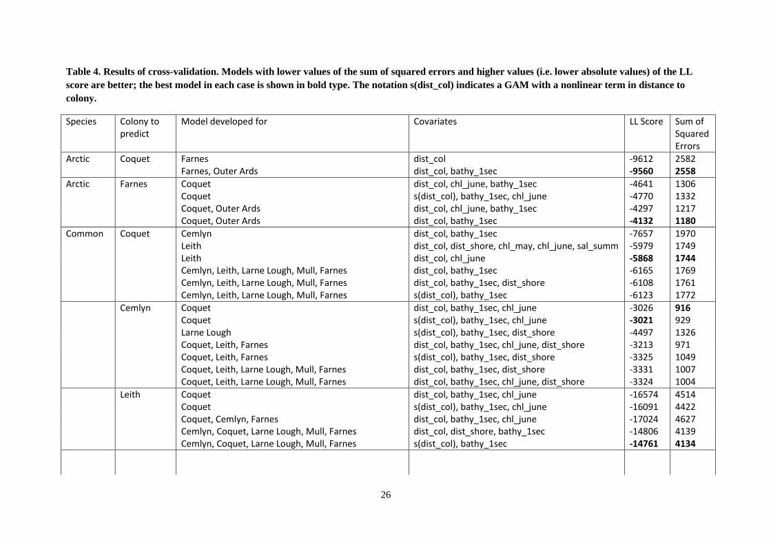
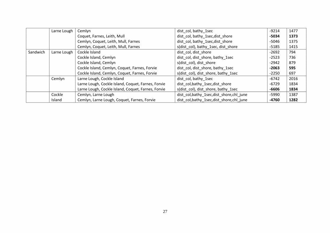
Table 4. Results of cross-validation. Models with lower values of the sum of squared errors and higher values (i.e. lower absolute values) of the LL

score are better; the best model in each case is shown in bold type. The notation s(dist_col) indicates a GAM with a nonlinear term in distance to

colony.

Species Colony to predict

Model developed for Covariates LL Score Sum of Squared Errors

Arctic Coquet Farnes dist_col -9612 2582 Farnes, Outer Ards dist_col, bathy_1sec -9560 2558

Arctic Farnes Coquet dist_col, chl_june, bathy_1sec -4641 1306 Coquet s(dist_col), bathy_1sec, chl_june -4770 1332 Coquet, Outer Ards dist_col, chl_june, bathy_1sec -4297 1217 Coquet, Outer Ards dist_col, bathy_1sec -4132 1180

Common Coquet Cemlyn dist_col, bathy_1sec -7657 1970 Leith dist_col, dist_shore, chl_may, chl_june, sal_summ -5979 1749 Leith dist_col, chl_june -5868 1744 Cemlyn, Leith, Larne Lough, Mull, Farnes dist_col, bathy_1sec -6165 1769 Cemlyn, Leith, Larne Lough, Mull, Farnes dist_col, bathy_1sec, dist_shore -6108 1761 Cemlyn, Leith, Larne Lough, Mull, Farnes s(dist_col), bathy_1sec -6123 1772

Cemlyn Coquet dist_col, bathy_1sec, chl_june -3026 916 Coquet s(dist_col), bathy_1sec, chl_june -3021 929 Larne Lough s(dist_col), bathy_1sec, dist_shore -4497 1326 Coquet, Leith, Farnes dist_col, bathy_1sec, chl_june, dist_shore -3213 971 Coquet, Leith, Farnes s(dist_col), bathy_1sec, dist_shore -3325 1049 Coquet, Leith, Larne Lough, Mull, Farnes dist_col, bathy_1sec, dist_shore -3331 1007 Coquet, Leith, Larne Lough, Mull, Farnes dist_col, bathy_1sec, chl_june, dist_shore -3324 1004

Leith Coquet dist_col, bathy_1sec, chl_june -16574 4514 Coquet s(dist_col), bathy_1sec, chl_june -16091 4422 Coquet, Cemlyn, Farnes dist_col, bathy_1sec, chl_june -17024 4627 Cemlyn, Coquet, Larne Lough, Mull, Farnes dist_col, dist_shore, bathy_1sec -14806 4139 Cemlyn, Coquet, Larne Lough, Mull, Farnes s(dist_col), bathy_1sec -14761 4134

27

Larne Lough Cemlyn dist_col, bathy_1sec -9214 1477 Coquet, Farnes, Leith, Mull dist_col, bathy_1sec,dist_shore -5034 1373 Cemlyn, Coquet, Leith, Mull, Farnes dist_col, bathy_1sec,dist_shore -5046 1375 Cemlyn, Coquet, Leith, Mull, Farnes s(dist_col), bathy_1sec, dist_shore -5185 1415

Sandwich Larne Lough Cockle Island dist_col, dist_shore -2692 794 Cockle Island, Cemlyn dist_col, dist_shore, bathy_1sec -2523 736 Cockle Island, Cemlyn s(dist_col), dist_shore -2942 879 Cockle Island, Cemlyn, Coquet, Farnes, Forvie dist_col, dist_shore, bathy_1sec -2063 595 Cockle Island, Cemlyn, Coquet, Farnes, Forvie s(dist_col), dist_shore, bathy_1sec -2250 697

Cemlyn Larne Lough, Cockle Island dist_col, bathy_1sec -6742 2016 Larne Lough, Cockle Island, Coquet, Farnes, Forvie dist_col,bathy_1sec,dist_shore -6729 1834 Larne Lough, Cockle Island, Coquet, Farnes, Forvie s(dist_col), dist_shore, bathy_1sec -6606 1834

Cockle Cemlyn, Larne Lough dist_col,bathy_1sec,dist_shore,chl_june -5990 1387 Island Cemlyn, Larne Lough, Coquet, Farnes, Forvie dist_col,bathy_1sec,dist_shore,chl_june -4760 1282

28

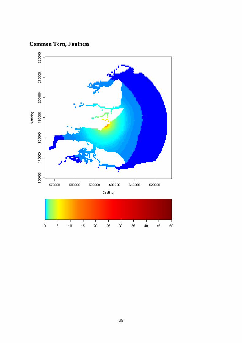
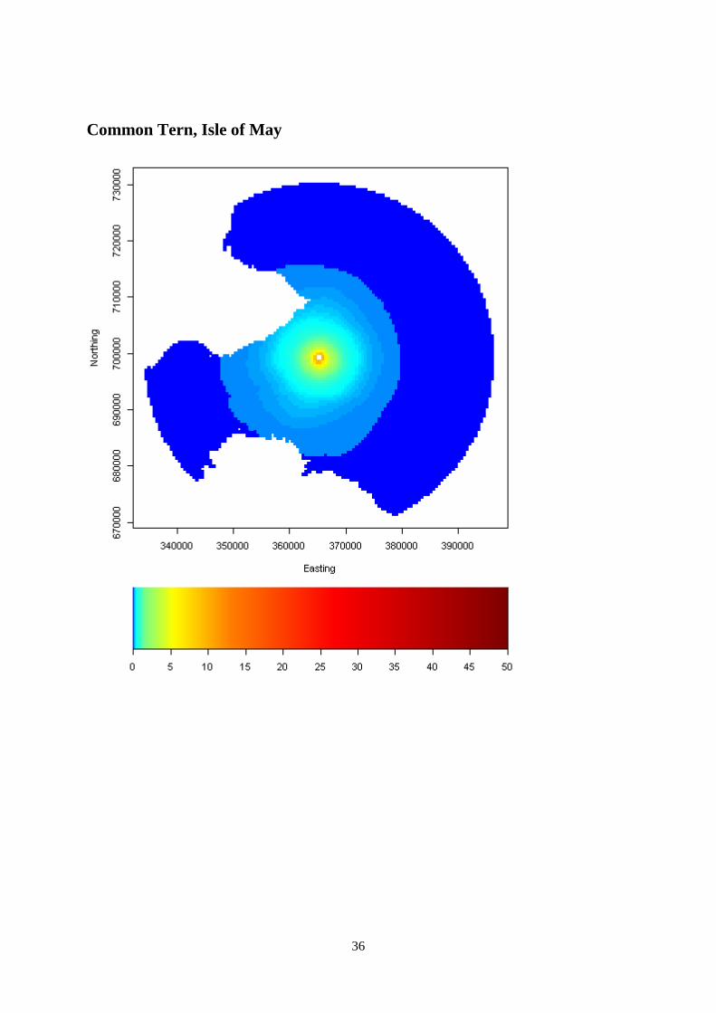
6. Prediction Maps of Usage

To calculate usage, preference is divided by distance to colony and multiplied by a scale factor which

ensures that the probabilities sum to one. For mapping purposes, the probabilities have been

multiplied by 1000. A very small number of points closest to the colony were removed if this gave a

value greater than 50.

Common Tern, Dungeness

29

Common Tern, Foulness

30

Common Tern, Breydon Water

31

Common Tern, Dee estuary

32

Common Tern, Ribble estuary

33

Common Tern, Strangford Lough

34

Common Tern, Carlingford Lough

35

Common Tern, Farne Islands

36

Common Tern, Isle of May

37

Arctic Tern, Strangford Lough

38

Arctic Tern, Isle of May

39

Sandwich Tern, Duddon estuary

40

Sandwich Tern, Strangford Lough

41

Sandwich Tern, Carlingford Lough

42

7. Discussion

Cross-validation has shown that it is generally better to combine all available data for a tern species

when making predictions for a new colony, rather than basing predictions on a colony or colonies that

appear to be ecologically similar. This means that the model developed for each species is more

robust, because it is based on data from a larger number of tracks, and covering a wider range of

environments. It might be possible to give the colonies differing weights, but it is unclear how such

weights should be chosen, as they would need to take account of the amount of data available for each

colony, as well as its ecological similarity to the colony being predicted which is difficult to measure

in relation to a terns assessment of its environment. The analysis has also shown that whereas the best

models for predicting the available data from a colony may involve many covariates and non-linear

terms, simple linear models with a small number of variables (in particular distance to colony,

distance to shore, bathymetry and chlorophyll concentration), are better for extrapolating to a different

colony.

43

References

Aarts, G., MacKenzie, M., McConnell, B., Fedak, M. and Matthiopoulos, J. (2008) Estimating space-

use and habitat preference from wildlife telemetry data. Ecography, 31, 140-160.

Brewer M.J., Potts J.M., Duff E.I. & Elston D.A. (2012). To carry out tern modelling under the

Framework Agreement C10-0206-0387. Report submitted to: Joint Nature Conservation Committee.

Brier, G.W. (1950) Verification of forecasts expressed in terms of probability. Monthly Weather

Review, 78, 1-3.

Chakraborty, A. Gelfand, A.E., Wilson A.M., Latimer A.M. and Silander J.A. Point pattern modelling

for degraded presence-only data over large regions. Applied Statistics 60, 757-776.

INLA (2012) R-Package, http://www.r-inla.org/

Liu C., White, M. and Newell G. (2011) Measuring and comparing the accuracy of species

distribution models with presence-absence data. Ecography 34, 232-243.

Lobo J.M., Jiménez-Valverde, A. and Real, R. (2008) AUC: A misleading measure of the

performance of predictive distribution models. Global Ecology and Biogeography, 17, 145-151.

Wakefield, E.D., Phillips, R.A., Trathan, P.N., Arata, J., Gales, R., Huin, N., Robertson, G., Waugh,

S.M., Weimerskirch, H. and Matthiopoulos, J. (2011) Habitat preference, accessibility, and

competition limit the global distribution of breeding Black-browed Albatrosses. Ecological

Monographs, 81, 141-167.

http://www.r-inla.org/

Biomathematics and Statistics Scotland

Prediction of New Colonies – Seabird Tracking

Data (Under Agreement C10-0206-0387)

CONTRACT No: C10-0206-0387

RESULTS APPENDIX

Submitted to:

Joint Nature Conservation Committee

October 2012

A. Results

This appendix contains detailed output and results from the Phase II analysis, and is supplement to the

Phase II report.

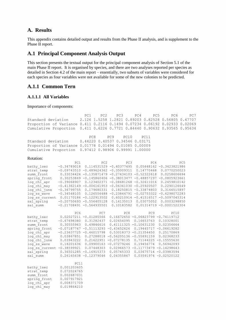
A.1 Principal Component Analysis Output

This section presents the textual output for the principal component analysis of Section 5.1 of the

main Phase II report. It is organised by species, and there are two analyses reported per species as

detailed in Section 4.2 of the main report – essentially, two subsets of variables were considered for

each species as four variables were not available for some of the new colonies to be predicted.

A.1.1 Common Tern

A.1.1.1 All Variables

Importance of components:

PC1 PC2 PC3 PC4 PC5 PC6 PC7

Standard deviation 2.126 1.5258 1.2821 0.89203 0.82528 0.56805 0.47707

Proportion of Variance 0.411 0.2116 0.1494 0.07234 0.06192 0.02933 0.02069

Cumulative Proportion 0.411 0.6226 0.7721 0.84440 0.90632 0.93565 0.95634

PC8 PC9 PC10 PC11

Standard deviation 0.44220 0.40537 0.34546 0.03171

Proportion of Variance 0.01778 0.01494 0.01085 0.00009

Cumulative Proportion 0.97412 0.98906 0.99991 1.00000

Rotation: PC1 PC2 PC3 PC4 PC5

bathy_1sec -0.34789018 0.114531529 -0.40377495 0.05648162 -0.3423821986

strat_temp -0.09743510 -0.489624362 -0.35009311 0.14770468 0.0770250023

summ_front 0.33034424 -0.135871479 -0.27434103 -0.52322618 0.0258606694

spring_front 0.30253849 -0.145860406 -0.38013477 -0.48857297 -0.0805923661

log_chl_apr -0.39068907 0.123402371 -0.08681268 -0.32611016 0.2459810142

log_chl_may -0.41362149 -0.006161953 -0.06361030 -0.25920507 0.2290126649

log_chl_june -0.36799755 0.179680331 0.18250815 -0.33874803 0.3166515897

log_ss_wave -0.34548105 0.126556488 -0.23844791 -0.02753322 -0.6298072283

log_ss_current 0.01170186 -0.122913502 0.60210914 -0.41516517 -0.5097045314

sal_spring -0.20750693 -0.556405128 0.14135013 0.03075052 0.0003298850

sal_summ -0.21708491 -0.564935501 0.10183582 0.01314719 -0.0001522304

PC6 PC7 PC8 PC9 PC10

bathy_1sec 0.02027211 -0.01285566 0.16672650 -0.06823799 -0.74119712

strat_temp -0.67698380 0.31282437 0.02654095 0.16653763 0.10328001

summ_front 0.30555963 0.49846616 0.41111325 -0.10631230 0.02356664

spring_front -0.07187747 -0.51113293 -0.43452626 0.19445717 -0.06619282

log_chl_apr -0.23637725 -0.46015798 0.53018373 -0.21354450 0.25170869

log_chl_may 0.03867851 0.27288018 -0.56205136 -0.55891159 0.02368233

log_chl_june 0.03943222 0.21622951 -0.07278135 0.71144225 -0.15555630

log_ss_wave 0.18201636 0.09900163 -0.07279246 0.19456774 0.56942093

log_ss_current -0.38599921 0.07448303 0.02966573 -0.11773479 -0.14298643

sal_spring 0.36501285 -0.16915373 0.05745333 0.03675714 -0.03983594

sal_summ 0.26165638 -0.12379046 0.04355867 0.03591974 -0.02520122

PC11

bathy_1sec 0.001203605

strat_temp 0.072024765

summ_front 0.002687031

spring_front 0.007917921

log_chl_apr 0.008371709

log_chl_may 0.019864210

log_chl_june 0.003167847

log_ss_wave 0.005181684

log_ss_current 0.018147376

sal_spring 0.677009898

sal_summ -0.731824969

A.1.1.2 Reduced Set of Variables

Importance of components:

PC1 PC2 PC3 PC4 PC5 PC6 PC7




Rotation:

PC1 PC2 PC3 PC4 PC5

bathy_1sec -0.36628037 -0.30889449 -0.26629352 0.76295247 -0.27662815

strat_temp 0.09048098 0.36518793 -0.88566451 -0.15922185 -0.12377532

summ_front 0.33978763 -0.56001521 -0.12040266 -0.27796552 -0.60160585

spring_front 0.32285029 -0.58616507 -0.22613592 -0.04298039 0.56172147

log_chl_apr -0.45668141 -0.30117855 -0.04310078 -0.15764595 0.06098516

log_chl_may -0.46151286 -0.13417700 -0.26139601 -0.22266652 0.37767922

log_chl_june -0.46520094 -0.07282486 0.09416116 -0.48888358 -0.29040513

PC6 PC7

bathy_1sec 0.006924129 -0.202096748

strat_temp -0.182563903 0.006916064

summ_front 0.289521828 0.182792828

spring_front -0.271388726 -0.331678424

log_chl_apr -0.498967488 0.649103924

log_chl_may 0.711104703 0.052750991

log_chl_june -0.233472257 -0.625752912

A.1.2 Sandwich Tern


Importance of components: PC1 PC2 PC3 PC4 PC5 PC6 PC7




PC8 PC9 PC10 PC11





bathy_1sec 0.300347363 -0.296482871 0.38307949 -0.01973168 0.44893437

strat_temp -0.001163675 0.458907292 0.43648019 0.01100438 0.15584748

summ_front -0.322000487 -0.196905358 0.21795174 0.47797601 -0.19503976

spring_front -0.299188824 -0.137454490 0.32033038 0.55817313 -0.06246183

log_chl_apr 0.344222464 -0.226669443 0.18226455 0.07794353 -0.44750208

log_chl_may 0.431054656 -0.003850706 0.11776160 0.15239735 -0.31170754

log_chl_june 0.408974633 -0.145965022 -0.23462344 0.09224658 -0.31115130

log_ss_wave 0.372426943 -0.248716291 0.21102848 0.10142341 0.44411667

log_ss_current 0.131993143 0.034224458 -0.59384214 0.57863770 0.37151183

sal_spring 0.210074053 0.503685288 0.06350888 0.18790402 -0.04593400

sal_summ 0.211611069 0.504387668 0.09627790 0.20308977 -0.02494160


bathy_1sec 0.07367752 -0.017152148 0.12495652 0.17164119 0.649849736

strat_temp -0.41334401 -0.003479685 -0.15234649 -0.60814631 0.080965489

summ_front -0.19505887 -0.678941342 0.20073549 0.05762667 0.030086604

spring_front 0.38623791 0.547758877 -0.08296824 -0.12741151 -0.033044644

log_chl_apr -0.60027800 0.387730138 0.19447365 0.19332394 -0.068531903

log_chl_may 0.16329126 -0.232032610 -0.76662381 0.09470947 0.046954905

log_chl_june 0.29728979 -0.096555000 0.36431504 -0.62848448 0.160082871

log_ss_wave 0.05705436 -0.124143590 0.07911575 -0.07484866 -0.718923109

log_ss_current -0.32706431 0.093454705 -0.14438251 -0.01709872 0.137164496

sal_spring 0.17795834 -0.021444453 0.28057598 0.29261301 -0.030056850

sal_summ 0.13862287 -0.024302771 0.22340982 0.21974761 -0.006848133

PC11

bathy_1sec 0.0102950910

strat_temp 0.0632935915

summ_front 0.0030573329


log_chl_apr -0.0043683231

log_chl_may 0.0230833626


log_ss_wave 0.0003777987


sal_spring 0.6806916231

sal_summ -0.7291241870







bathy_1sec 0.3606380 0.29914738 0.3034279 0.79331732 -0.1359515

strat_temp -0.1114965 -0.53193530 0.7473371 -0.06903824 0.1198148

summ_front -0.3288831 0.53543377 0.1809402 -0.24658846 0.2156151

spring_front -0.3310363 0.48096817 0.3840976 -0.12884764 -0.4291506

log_chl_apr 0.4282324 0.30529009 0.1914374 -0.17302966 0.7187831

log_chl_may 0.4695898 -0.04435079 0.3288154 -0.35913617 -0.3373342

log_chl_june 0.4856562 0.11986218 -0.1561430 -0.35993848 -0.3256655

PC6 PC7

bathy_1sec 0.17586598 0.098073924

strat_temp 0.05146465 0.352604874

summ_front 0.67458247 0.100249385

spring_front -0.55740891 0.008775335

log_chl_apr -0.37290473 -0.033472053

log_chl_may 0.24261168 -0.606436520

log_chl_june 0.05232566 0.697881602

A.1.3 Arctic Tern






PC8 PC9 PC10 PC11





bathy_1sec -0.333836387 0.013161993 -0.4829602728 -0.29884043 0.01879676

strat_temp -0.155694546 -0.533598541 -0.0791227678 -0.08359333 -0.28080338

summ_front 0.284012176 -0.309210371 -0.0048270382 -0.01330141 0.67150701

spring_front 0.263354007 -0.371690597 -0.1853294130 -0.06105639 0.40242120

log_chl_apr -0.387899409 0.083121698 -0.0009342481 0.29803032 0.29024743

log_chl_may -0.413888043 0.008451205 0.0693954594 0.04731083 0.26997113

log_chl_june -0.334075856 0.271278318 0.2736367785 0.22665728 0.31999929

log_ss_wave -0.339050144 0.065397063 -0.3582628866 -0.50870864 0.15981678

log_ss_current 0.003913797 0.059759942 0.6480111024 -0.69383431 0.08499806

sal_spring -0.287770094 -0.437110380 0.2257176401 0.11242479 -0.08812236

sal_summ -0.288333731 -0.449275338 0.2172690589 0.06736447 -0.08872710


bathy_1sec -0.09324483 0.20614144 -0.18796922 0.25393482 0.64378635

strat_temp 0.06948954 0.09208073 0.55983853 -0.48692242 0.17608113

summ_front -0.56138198 0.20998889 0.09991796 -0.05220779 0.02540537

spring_front 0.69602423 -0.26231843 -0.17407394 0.01574098 0.09278359

log_chl_apr 0.36137733 0.69406928 0.08362277 0.01158837 -0.22370499

log_chl_may -0.00870916 -0.44772429 0.55439647 0.48878603 -0.03756157

log_chl_june -0.01121842 -0.28911261 -0.16929262 -0.56845975 0.38809631

log_ss_wave -0.08290671 -0.16260268 -0.13800296 -0.31387250 -0.56317764

log_ss_current 0.16544059 0.20100026 0.05338970 0.06458366 0.11201638

sal_spring -0.11432111 -0.03783720 -0.39465065 0.14317052 -0.09477405

sal_summ -0.09364001 -0.04552860 -0.30051695 0.10036368 -0.06714130

PC11

bathy_1sec 0.002323419

strat_temp 0.064094992

summ_front 0.002095481


log_chl_apr -0.007848587

log_chl_may 0.021813060


log_ss_wave 0.006860233


sal_spring 0.674566177

sal_summ -0.734619937







bathy_1sec -0.32230893 0.06226992 0.53537600 -0.7138865 0.23258760

strat_temp -0.01577292 0.91263966 -0.05688776 0.1186194 -0.09540982

summ_front 0.38633145 -0.07003159 0.52270480 0.3688866 0.35579893

spring_front 0.40106797 0.09722610 0.53519002 0.1118030 -0.25452978

log_chl_apr -0.43269042 -0.10340998 0.34557456 0.1993234 -0.73584324

log_chl_may -0.44760165 0.28589533 0.17111802 0.2810857 0.37300508

log_chl_june -0.44518807 -0.23753779 0.04224325 0.4571425 0.25460484

PC6 PC7

bathy_1sec -0.04595519 0.19942184

strat_temp -0.14907359 0.34381291

summ_front -0.55636260 0.02034051

spring_front 0.68171514 0.03524727

log_chl_apr -0.30459808 -0.09321230

log_chl_may 0.21506648 -0.65133684

log_chl_june 0.24971332 0.63830972

A.1 Arctic Terns

Call:

glm(formula = SEARCH_FORAGE ~ dist_col + bathy_1sec, family = "binomial",

data = complete.data.to.analyse, weights = weights)

Deviance Residuals:

Min 1Q Median 3Q Max

-0.11201 -0.06439 -0.03924 -0.01965 0.54334

Coefficients:

Estimate Std. Error z value Pr(>|z|)

(Intercept) -1.324605 0.156462 -8.466 < 2e-16 ***

dist_col -0.188299 0.022905 -8.221 < 2e-16 ***

bathy_1sec -0.016695 0.003754 -4.447 8.69e-06 ***

---

Signif. codes: 0 ‘***’ 0.001 ‘**’ 0.01 ‘*’ 0.05 ‘.’ 0.1 ‘ ’ 1

(Dispersion parameter for binomial family taken to be 1)

Null deviance: 966.19 on 94340 degrees of freedom

Residual deviance: 843.07 on 94338 degrees of freedom

AIC: 6

Number of Fisher Scoring iterations: 7

Model:

SEARCH_FORAGE ~ dist_col + bathy_1sec

Df Deviance AIC LRT Pr(>Chi)

<none> 843.07 6.000

dist_col 1 949.11 110.041 106.041 < 2.2e-16 ***

bathy_1sec 1 861.77 22.698 18.698 1.532e-05 ***

---

Signif. codes: 0 ‘***’ 0.001 ‘**’ 0.01 ‘*’ 0.05 ‘.’ 0.1 ‘ ’ 1

A.2 Common Terns

Call:

glm(formula = SEARCH_FORAGE ~ dist_col + bathy_1sec + dist_shore,

family = "binomial", data = complete.data.to.analyse, weights = weights)

Deviance Residuals:


-0.16299 -0.07414 -0.03977 -0.01809 0.51218

Coefficients:


(Intercept) -0.969564 0.116431 -8.327 < 2e-16 ***

dist_col -0.159943 0.016617 -9.625 < 2e-16 ***

bathy_1sec -0.008479 0.002167 -3.914 9.1e-05 ***

dist_shore -0.078295 0.030170 -2.595 0.00945 **

---

Signif. codes: 0 ‘***’ 0.001 ‘**’ 0.01 ‘*’ 0.05 ‘.’ 0.1 ‘ ’ 1




AIC: 8


Model:

SEARCH_FORAGE ~ dist_col + bathy_1sec + dist_shore


<none> 1577.7 8.000

dist_col 1 1730.2 158.503 152.503 < 2.2e-16 ***

bathy_1sec 1 1591.6 19.940 13.940 0.0001888 ***

dist_shore 1 1584.8 13.175 7.175 0.0073946 **

---

Signif. codes: 0 ‘***’ 0.001 ‘**’ 0.01 ‘*’ 0.05 ‘.’ 0.1 ‘ ’ 1

A.3 Sandwich Terns

Call:

glm(formula = SEARCH_FORAGE ~ dist_col + chl_june + bathy_1sec +

dist_shore, family = "binomial", data = complete.data.to.analyse,

weights = weights)

Deviance Residuals:


-0.20316 -0.03220 -0.00938 -0.00320 0.54600

Coefficients:


(Intercept) -0.645190 0.389714 -1.656 0.097814 .

dist_col -0.055307 0.008268 -6.689 2.25e-11 ***

chl_june 0.429606 0.176824 2.430 0.015117 *

bathy_1sec 0.021380 0.006717 3.183 0.001458 **

dist_shore -0.136294 0.041395 -3.293 0.000993 ***

---

Signif. codes: 0 ‘***’ 0.001 ‘**’ 0.01 ‘*’ 0.05 ‘.’ 0.1 ‘ ’ 1




AIC: 10


Model:

SEARCH_FORAGE ~ dist_col + chl_june + bathy_1sec + dist_shore


<none> 950.59 10.000

dist_col 1 1017.34 74.742 66.742 3.094e-16 ***

chl_june 1 956.43 13.839 5.839 0.0156709 *

bathy_1sec 1 962.31 19.713 11.713 0.0006205 ***

dist_shore 1 965.15 22.558 14.558 0.0001359 ***

---

Signif. codes: 0 ‘***’ 0.001 ‘**’ 0.01 ‘*’ 0.05 ‘.’ 0.1 ‘ ’ 1

Excluding chl_june

Call:

glm(formula = SEARCH_FORAGE ~ dist_col + bathy_1sec + dist_shore,

family = "binomial", data = complete.data.to.analyse, weights = weights)

Deviance Residuals:


-0.18731 -0.03325 -0.00869 -0.00262 0.57833

Coefficients:


(Intercept) 0.231125 0.148744 1.554 0.120222

dist_col -0.053509 0.008093 -6.612 3.80e-11 ***

bathy_1sec 0.027722 0.006408 4.326 1.52e-05 ***

dist_shore -0.160435 0.041284 -3.886 0.000102 ***

---

Signif. codes: 0 ‘***’ 0.001 ‘**’ 0.01 ‘*’ 0.05 ‘.’ 0.1 ‘ ’ 1




AIC: 8


Prediction of New Colonies – Seabird Tracking Data (Under...

Documents

Transcript of Prediction of New Colonies – Seabird Tracking Data (Under...