Prediction of Functional Quantitative Traits in Plants...

Prediction of Functional Quantitative Traits in Plants using a Whole-Genome Population-

Based ApproachTatiana Tatarinova

What is the SNP

• SINGLE • NUCLEOTIDE • POLIMORPHISM

Human genome has about 3 billion nucleotides Two randomly selected individuals differ by

<0.5% of a genome (<15 mil)

Why do we care about SNPs?

• History • Personalized medicine • Clinical trials • Forensics • Agriculture and breeding • Monitoring rare species

DNA

…TCAGGTCACAGTCT…

…TCAGGTCACAGTCT……TCAGGCCACAGTCT……TCAGGCCACAGTCT…

Individual 1

Individual 2

Individual 3

DNA

Reference sequence

Katarzyna Bryc, 2013

Single Nucleotide Polymorphism (SNP)

…TCAGGTCACAGTCT……TCAGGCCACAGTCT……TCAGGCCACAGTCT…

SNP A.k.a. allele, locus, marker, variant


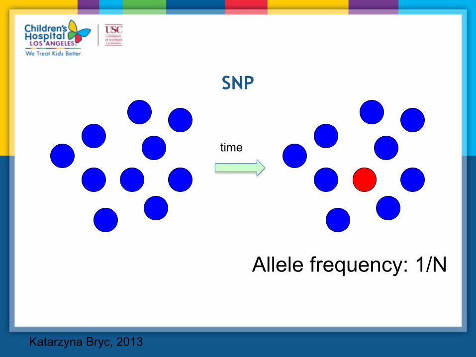
SNP

Allele frequency: 1/N

time


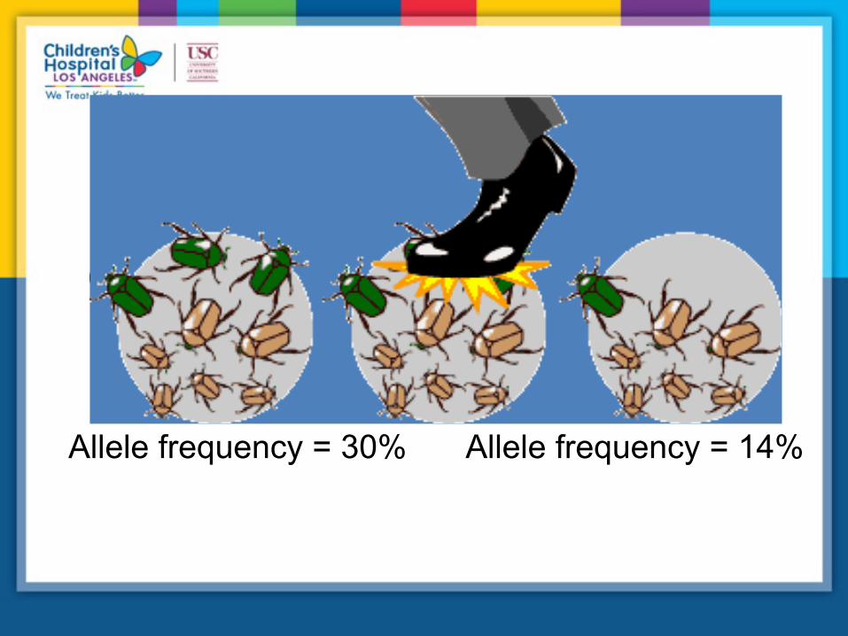
Genetic drift

Allele frequency = 30% Allele frequency = 14%

time

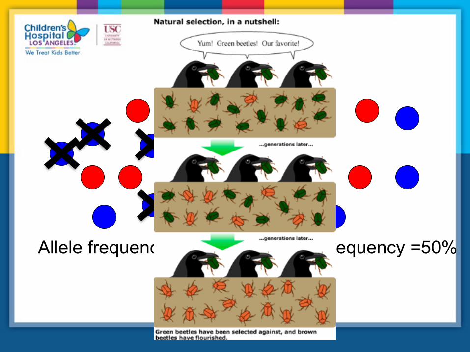
Natural selection

Allele frequency = 30% Allele frequency =50%

Population structure

67%

30%

17%

Population 1

Population 2

Barrier

Pigmentation example - SLC45A2

ALFRED: The ALlele FREquency Database

http://alfred.med.yale.edu/alfred/Katarzyna Bryc, 2013

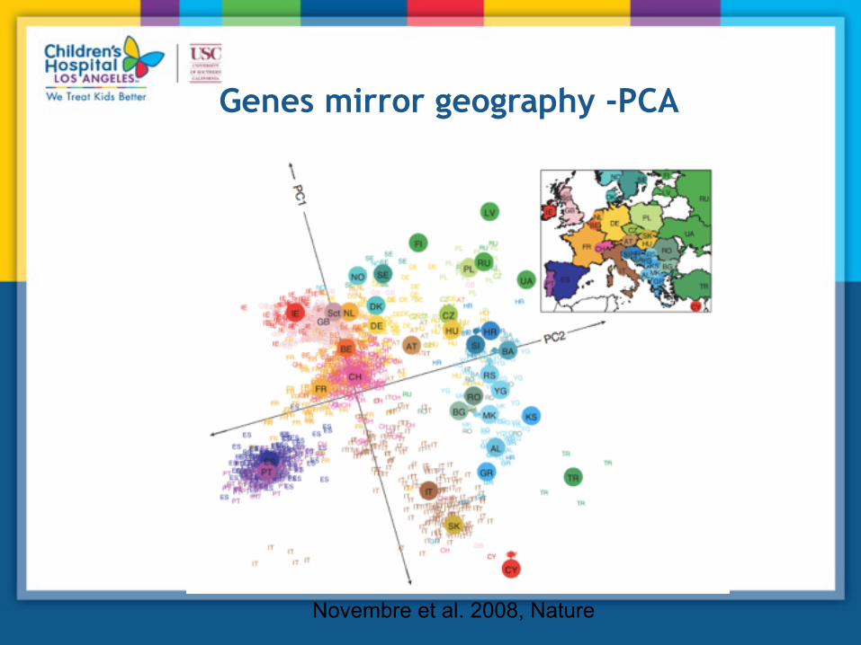
Genes mirror geography -PCA

Novembre et al. 2008, Nature

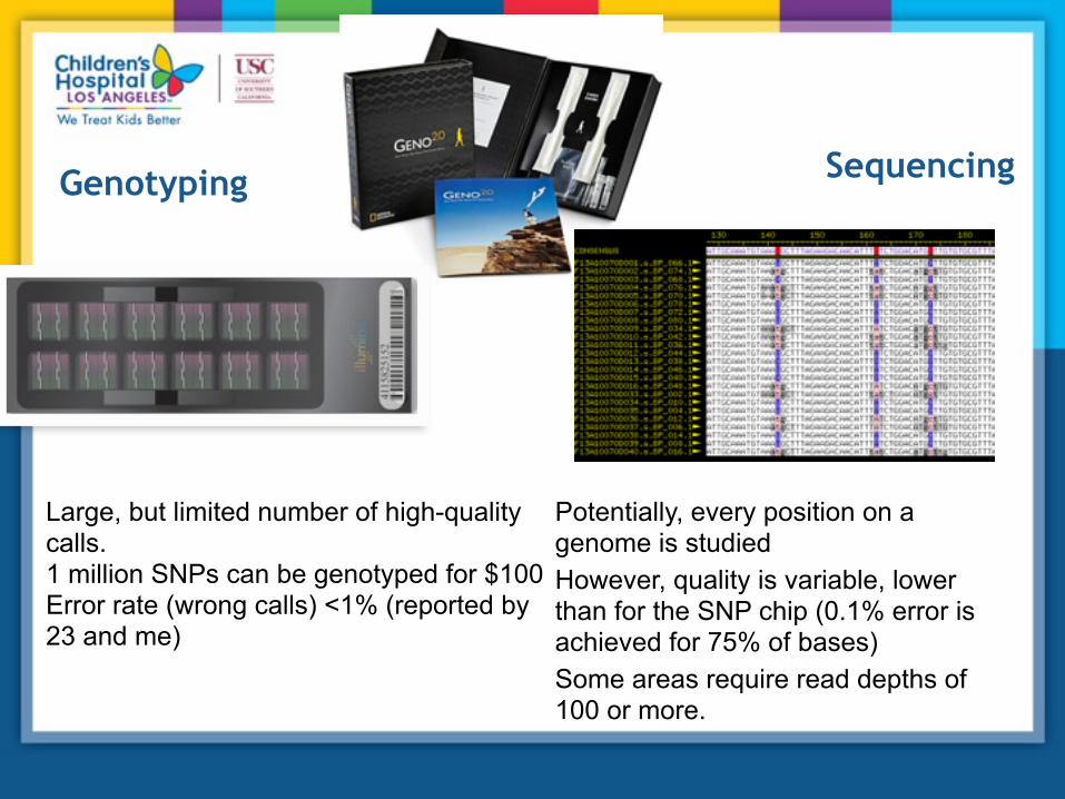
Genotyping Sequencing

Potentially, every position on a genome is studied However, quality is variable, lower than for the SNP chip (0.1% error is achieved for 75% of bases) Some areas require read depths of 100 or more.

Large, but limited number of high-quality calls. 1 million SNPs can be genotyped for $100 Error rate (wrong calls) <1% (reported by 23 and me)

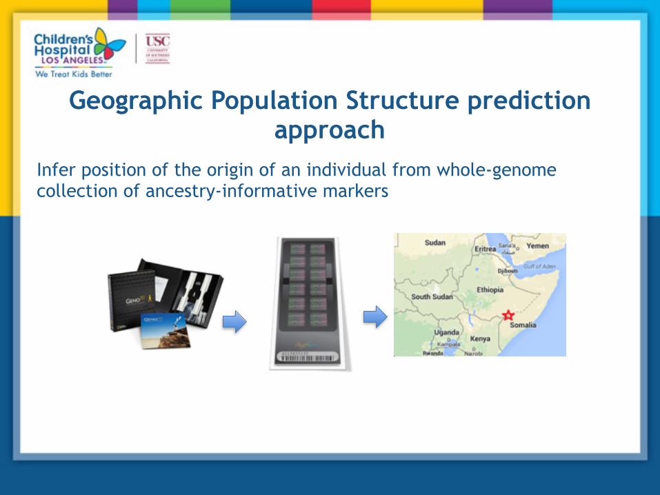
Geographic Population Structure prediction approach

Infer position of the origin of an individual from whole-genome collection of ancestry-informative markers

National Genographic Project

• Goal: Assemble world-wide collection of reference genotypes • How is it done?

Machu Picchu

Solstice festival in Cusco

Uros people

Taquile island, Titicaca lake

Amazon river

Urarina

IMG_1947.CR2

~700 km

Turuhansk

Bor

Kellog

Nganasan

300 km

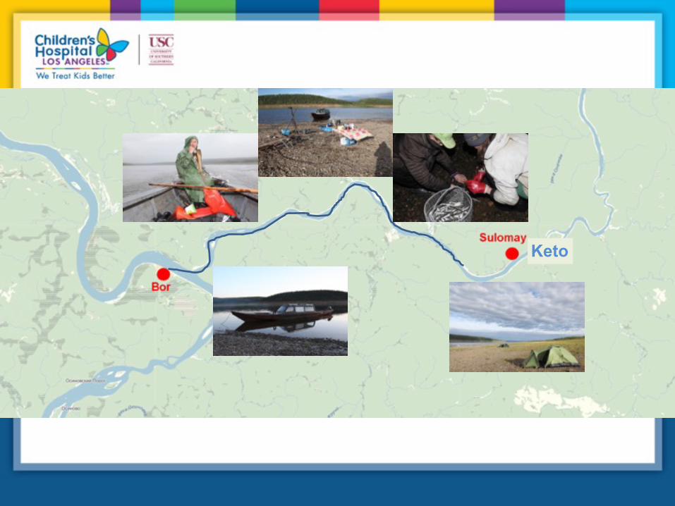
67 km

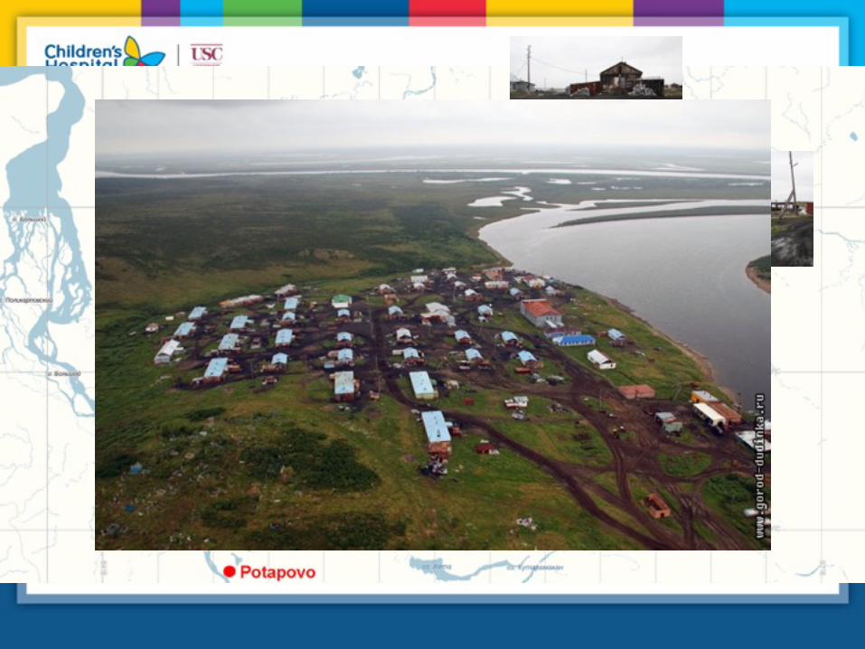
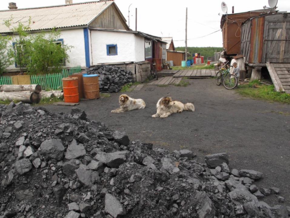
Keto

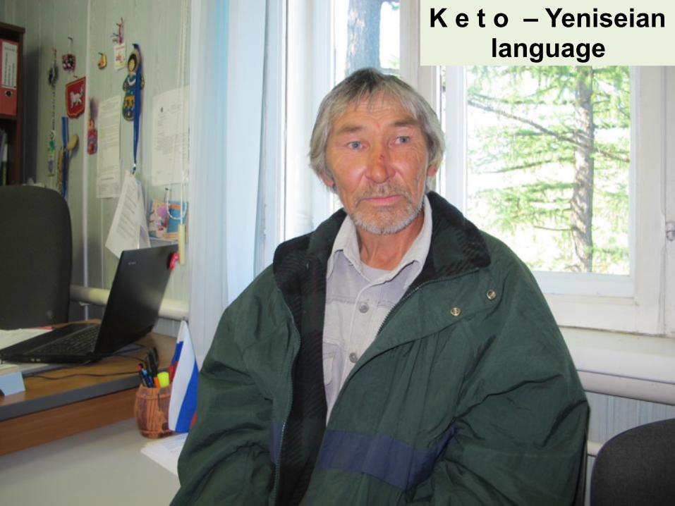
K e t o – Yeniseian language

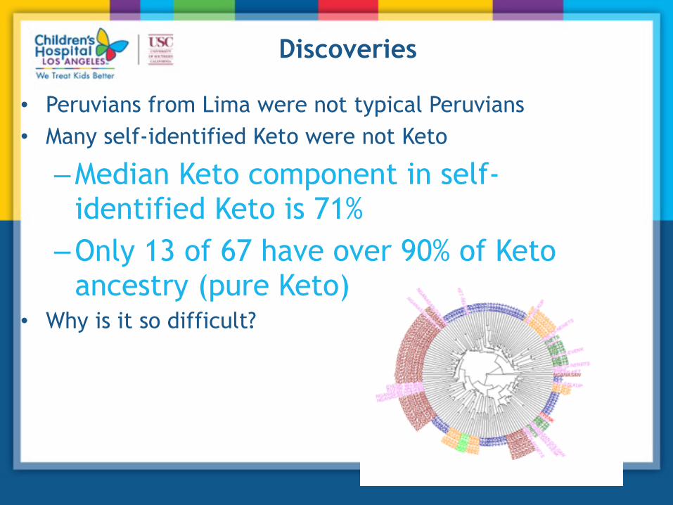
Discoveries

• Peruvians from Lima were not typical Peruvians • Many self-identified Keto were not Keto

–Median Keto component in self-identified Keto is 71%

–Only 13 of 67 have over 90% of Keto ancestry (pure Keto)

• Why is it so difficult?

How to collect data

• Approach village nurse, elders, shamans • Request to select unrelated people of “pure” origin, who remember

their grandparents • Distribute a survey requesting information about place of birth and

ethnicity of the individual, his/her parents and grandparents

All >75% <=75%

• In pairs

– Obtain informed consent • Find out:

– Parents’ names – Parents’ dates of birth – Parents’ place of birth – Parents’ ethnicities

• Then:

– Grandparents’ names – Grandparents’ dates of birth – Grandparents’ place of birth – Grandparents’ ethnicities

Exercise

How to find Ancestry Informative Markers (AIMs)?

• How to find Ancestry Informative Markers? • For each position on the genome, we have information from K

populations. Each locus can have up to N alleles. • In - informativeness for assignment. For a given set of populations,

the minimal of In=0 occurs when all alleles have equal frequencies in all populations. The maximal value, log(K), occurs when N > K and no allele is found in more than one population

Example: K=2 and N=2

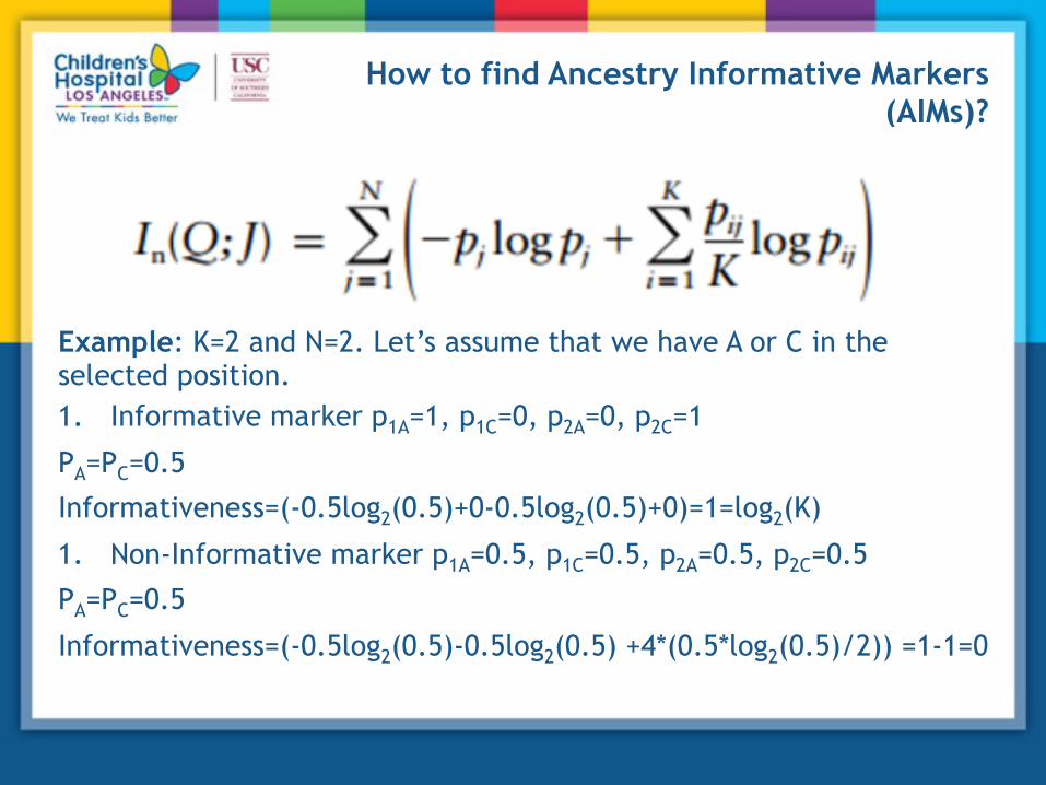
How to find Ancestry Informative Markers (AIMs)?

Example: K=2 and N=2. Let’s assume that we have A or C in the selected position. 1. Informative marker p1A=1, p1C=0, p2A=0, p2C=1

PA=PC=0.5

Informativeness=(-0.5log2(0.5)+0-0.5log2(0.5)+0)=1=log2(K)

1. Non-Informative marker p1A=0.5, p1C=0.5, p2A=0.5, p2C=0.5

PA=PC=0.5

Informativeness=(-0.5log2(0.5)-0.5log2(0.5) +4*(0.5*log2(0.5)/2)) =1-1=0

HOW TO PROCESS SAMPLES

To infer population structure from genotype data, it is necessary to first reduce the dimensionality of the dataset due to the thousands of SNPs it encompasses.

From SNPs to Admixture

Thousands of ancestry informative SNPs

North East Asian Mediterranian South African

South West Asian

Native American Oceanian

South East Asian

Northern European

Sub-Saharan African

HGDP00985 0.5253 0.0202 0 0.2222 0.0404 0.0101 0.0101 0.1717 0

HGDP01094 0.04 0.04 0 0.03 0.83 0 0.01 0.05 0

HGDP00982 0.0102 0.1531 0.0306 0.0714 0.0408 0 0.0102 0.2041 0.4796

ADMIXTURE

Admixture proportions in geographically adjacent populations, such as Italian and Greeks, and populations sharing similar history, like British and Germans, are similar.

36

Selection of K

Identify the best K value as judged by prediction of systematically withheld data points

Question

• How to link genetic and geographic divergence?

39

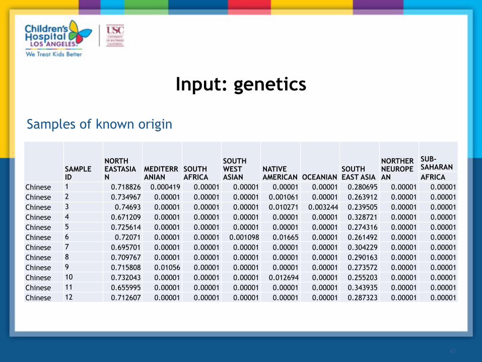
Input: genetics

Samples of known origin

40

SAMPLE ID

NORTH EASTASIAN

MEDITERRANIAN

SOUTH AFRICA

SOUTH WEST ASIAN

NATIVE AMERICAN OCEANIAN

SOUTH EAST ASIA

NORTHERNEUROPEAN

SUB-SAHARANAFRICA

Chinese 1 0.718826 0.000419 0.00001 0.00001 0.00001 0.00001 0.280695 0.00001 0.00001Chinese 2 0.734967 0.00001 0.00001 0.00001 0.001061 0.00001 0.263912 0.00001 0.00001Chinese 3 0.74693 0.00001 0.00001 0.00001 0.010271 0.003244 0.239505 0.00001 0.00001Chinese 4 0.671209 0.00001 0.00001 0.00001 0.00001 0.00001 0.328721 0.00001 0.00001Chinese 5 0.725614 0.00001 0.00001 0.00001 0.00001 0.00001 0.274316 0.00001 0.00001Chinese 6 0.72071 0.00001 0.00001 0.001098 0.01665 0.00001 0.261492 0.00001 0.00001Chinese 7 0.695701 0.00001 0.00001 0.00001 0.00001 0.00001 0.304229 0.00001 0.00001Chinese 8 0.709767 0.00001 0.00001 0.00001 0.00001 0.00001 0.290163 0.00001 0.00001Chinese 9 0.715808 0.01056 0.00001 0.00001 0.00001 0.00001 0.273572 0.00001 0.00001Chinese 10 0.732043 0.00001 0.00001 0.00001 0.012694 0.00001 0.255203 0.00001 0.00001Chinese 11 0.655995 0.00001 0.00001 0.00001 0.00001 0.00001 0.343935 0.00001 0.00001Chinese 12 0.712607 0.00001 0.00001 0.00001 0.00001 0.00001 0.287323 0.00001 0.00001

For every reference population, calculate mean admixture vectors

NORTH EAST ASIA

MEDI-TERRANIA

SOUTH AFRICA

SOUTH WEST ASIA

NATIVE AMERICA OCEANIA

SOUTH EAST ASIA

NORTHERN EUROPE

SUB-SAHARANAFRICA

Chinese 0.711681 0.000923 1.00E-05 0.000101 0.003396 0.00028 0.283589 1.00E-05 1.00E-05

Russian 0.068867 0.265222 0.001241 0.224659 0.035011 0.008622 0.031844 0.363107 0.001419

Tatar 0.15794 0.209897 1.00E-05 0.210957 0.011902 0.002605 0.005703 0.400975 1.00E-05

41

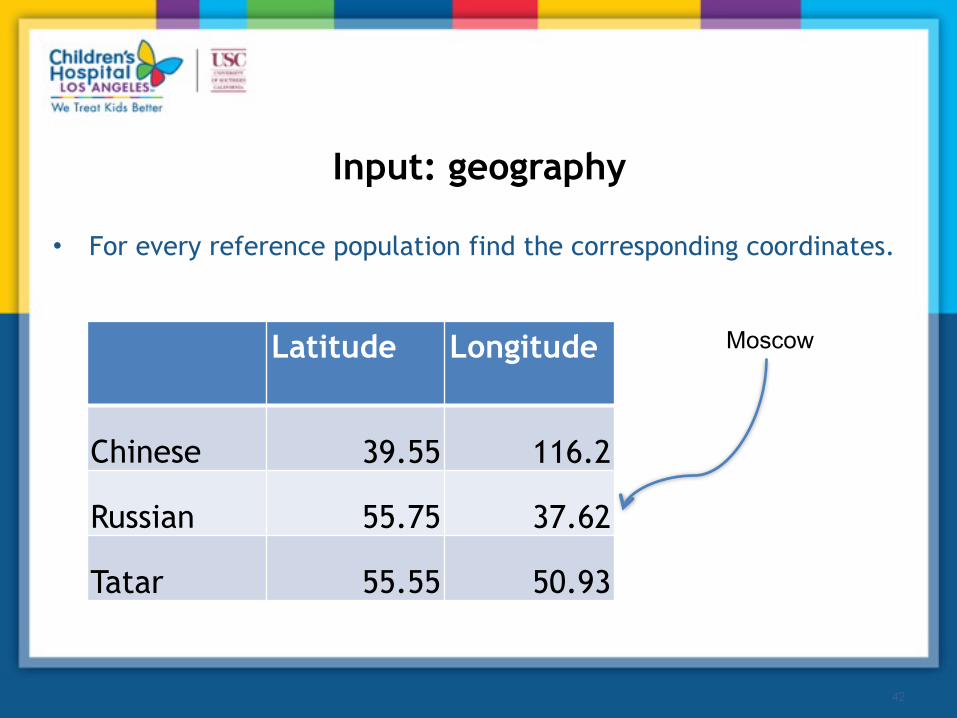
Input: geography

• For every reference population find the corresponding coordinates.

Latitude Longitude

Chinese 39.55 116.2

Russian 55.75 37.62

Tatar 55.55 50.93

Moscow

42

Prediction of provenance

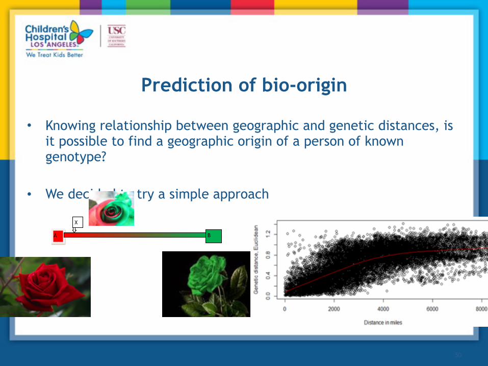
• Knowing relationship between geographic and genetic distances, is it possible to find a geographic origin of a person of known genotype?

• We decided to try a simple approach

43

A B

X

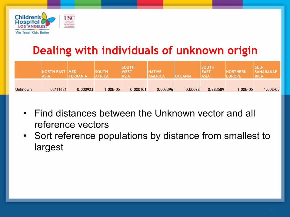
Dealing with individuals of unknown origin

NORTH EAST ASIA

MEDI-TERRANIA

SOUTH AFRICA

SOUTH WEST ASIA

NATIVE AMERICA OCEANIA

SOUTH EAST ASIA

NORTHERN EUROPE

SUB-SAHARANAFRICA

Unknown 0.711681 0.000923 1.00E-05 0.000101 0.003396 0.00028 0.283589 1.00E-05 1.00E-05

• Find distances between the Unknown vector and all reference vectors

• Sort reference populations by distance from smallest to largest

44

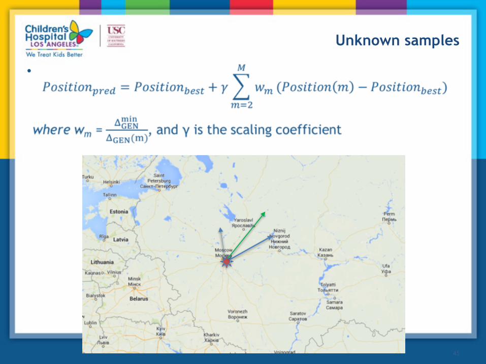
Unknown samples

•

45

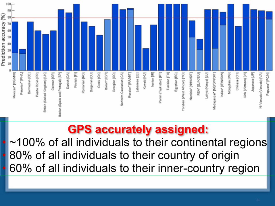
GPS accurately assigned: • ~100% of all individuals to their continental regions • 80% of all individuals to their country of origin • 60% of all individuals to their inner-country region

46

True Predicted

GPS

SPA

47

.

GPS achieved high assignment accuracy for Southeast Asian and Oceanian populations (87.5%) and subpopulations (77%).

We traced the origins of Remote Oceanian populations to Near Oceania.

Reich et al. (2011). Denisova admixture and the first modern human dispersals into Southeast Asia and Oceania, AJHG

243 Southeast Asian and Oceanian samples

48

OTHER ORGANISMS WHOGEM

Application of GPS to

Prediction of bio-origin

• Knowing relationship between geographic and genetic distances, is it possible to find a geographic origin of a person of known genotype?

• We decided to try a simple approach

50

A B

X

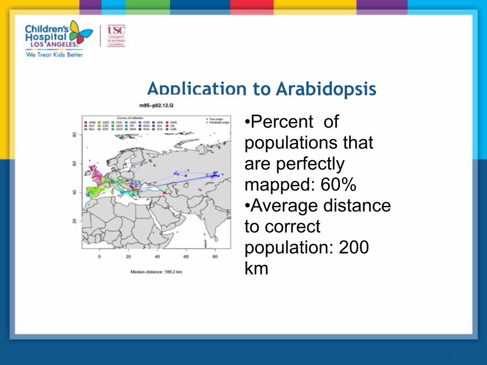
Application to Arabidopsis

51

•Percent of populations that are perfectly mapped: 60% •Average distance to correct population: 200 km

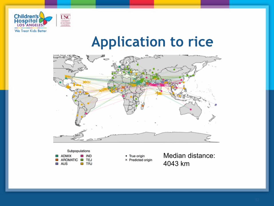
Application to rice

52

Median distance: 4043 km

■Legumes (fabaceae) plant family Ability to establish nodule symbiosis High synteny to legume crops

■Small diploid genome (500Mb) sequenced Tang et al., 2014 (BMC Genomics)

■Numerous genomic resources • RIL populations • Mutant collections • Large EST and RNASEQ databases • HAPMAP resources Branca et al., 2011

(PNAS) • 288 genomes already sequenced

■Biotechnology tools for validation ■Large biodiversity Gentzbittel et al., 2015 (Front. Pl. Sci)

Medicago truncatula

M. truncatula - a model legume plant

01/08/2017

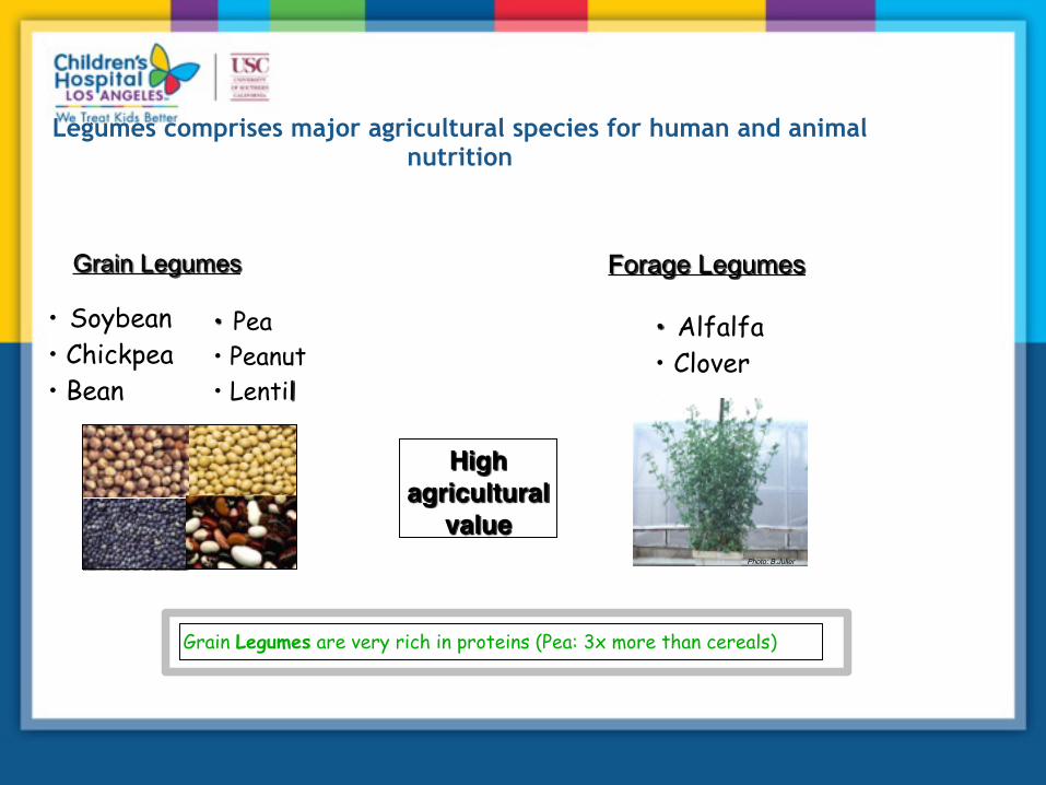
Grain Legumes Forage Legumes

• Alfalfa • Clover

• Soybean • Chickpea • Bean

High agricultural

value

• Pea • Peanut • Lentil

Grain Legumes are very rich in proteins (Pea: 3x more than cereals)

Photo: B.Julier

Legumes comprises major agricultural species for human and animal nutrition

HapMap data for M. truncatulaCurrent state: 288 sequenced accessions

# SNPs Chr1 : 1.508.346 Chr2 : 1.964.419 Chr3 : 2.472.365 Chr4 : 2.225.537 Chr5 : 3.251.290 Chr6 : 1.172.980 Chr7 : 2.262.094 Chr8 : 1.659.690

Total : 16.516.721 ~ 40% of SNPs in coding regions

18 sister taxa

Here are the data available for the 288 Medicago accessions that have been already sequenced leading to a total number of more than 16.5 million SNP. Among those, 18 accessions which highly diverged from others have been re-classified to some sister taxa despite perfect botanic similarities

56

M. truncatula is spontaneously occurring all around the Mediterranean basin

Several collections are available: DZ, TN, FR , AU, US, …. for thousands of accessions

Photo: A.Abdelguerfi, INA, Alger, AlgeriaPhoto: J-M Prospéri, INRA Montpellier, France

Photo: J-M Prospéri, INRA Montpellier, France Photo: E.Aouani, CBBC, Tunisia Photo: L. Gentzbittel, ENSAT, Toulouse, France

Photo: L. Gentzbittel, ENSAT, Toulouse, France

57

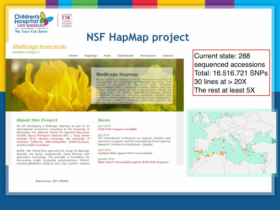
NSF HapMap project

Current state: 288 sequenced accessions Total: 16.516.721 SNPs 30 lines at > 20XThe rest at least 5X

Branca et al., 2011 (PNAS)

58

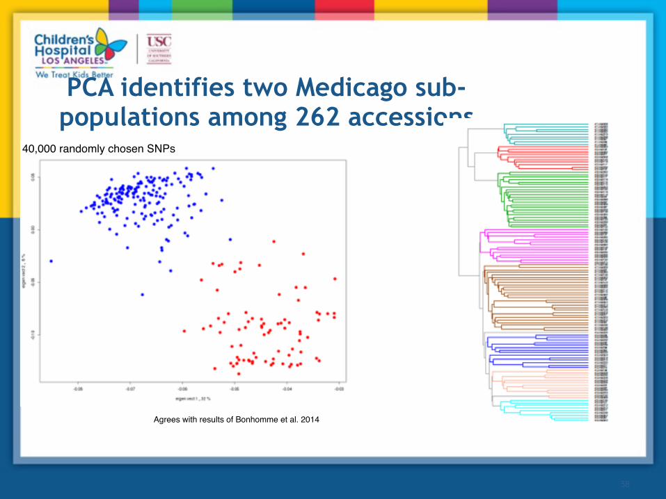
PCA identifies two Medicago sub-populations among 262 accessions

Agrees with results of Bonhomme et al. 2014

40,000 randomly chosen SNPs

A refined population structure for Medicago species using GPS algorithm

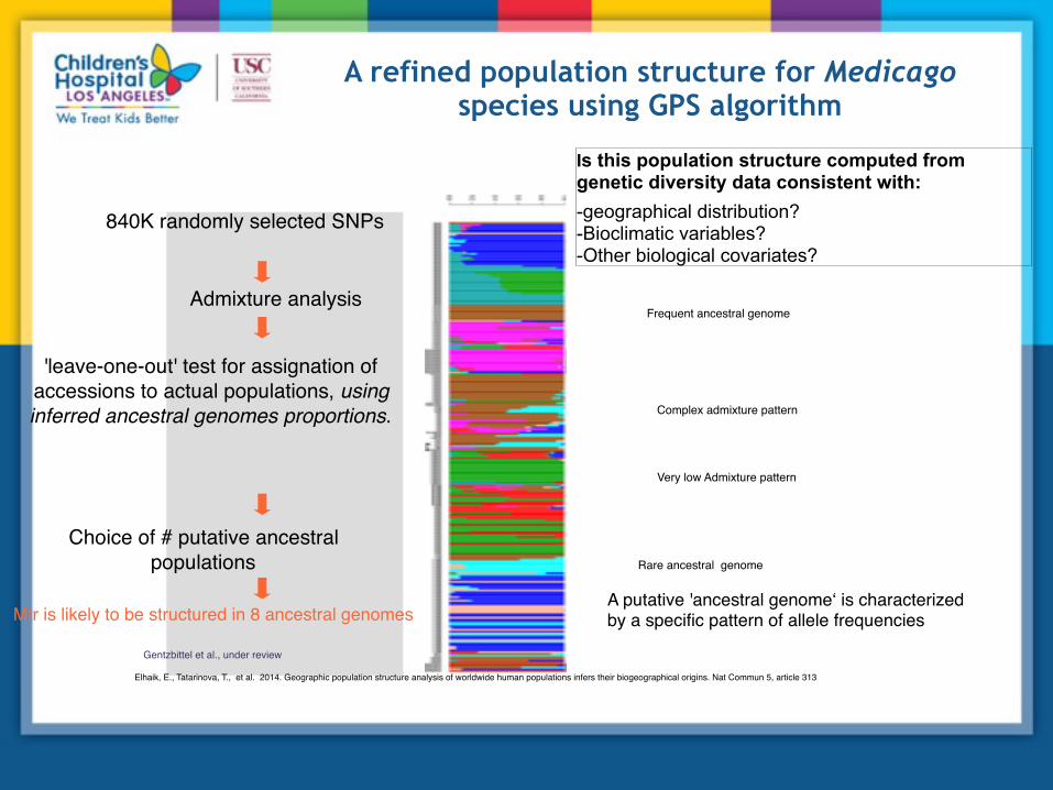
Medicago is likely to be structured in 8 ancestral genomesElhaik, E., Tatarinova, T., et al. 2014. Geographic population structure analysis of worldwide human populations infers their biogeographical origins. Nat Commun 5, article 313

Fig. 2: Predicted distance from true origin for each M. truncatula accession using t h e l e a v e - o n e - o u t procedure, for increasing values of K.

'leave-one-out' test for assignation of accessions to actual populations, using inferred ancestral genomes proportions.

840K randomly selected SNPs (~100,000 per chromosome)

Admixture analysis

Choice of # putative ancestral populations

Fig. 1: BIC as a function of increasing values of K, using Discriminant Analysis of Principal Components (DAPC) applied on the 8 4 0 K S N P d a t a s e t . (Jombart et al 2010)

K=8

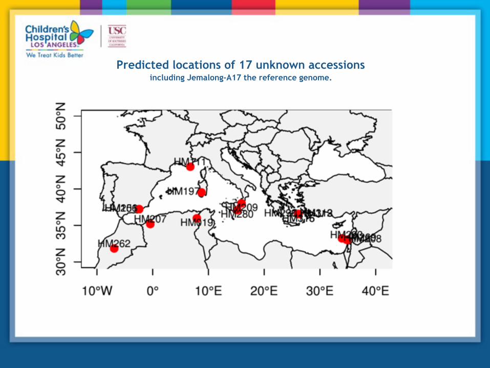
Predicted locations of 17 unknown accessions including Jemalong-A17 the reference genome.

Examples of GPS analysis with various levels of accuracy

'Leave-one Out' procedure accuracy is <300 kilometers

Linear relationship between geographical and genetic distances when d < 950 km (R=0.8, p-value=10-4, Mantel's test)

A refined population structure for Medicago species using GPS algorithm

Mtr is likely to be structured in 8 ancestral genomes

Elhaik, E., Tatarinova, T., et al. 2014. Geographic population structure analysis of worldwide human populations infers their biogeographical origins. Nat Commun 5, article 313

'leave-one-out' test for assignation of accessions to actual populations, using inferred ancestral genomes proportions.

840K randomly selected SNPs

Admixture analysis

Choice of # putative ancestral populations Rare ancestral genome

Complex admixture pattern

Very low Admixture pattern

Frequent ancestral genome

A putative 'ancestral genome‘ is characterized by a specific pattern of allele frequencies

Gentzbittel et al., under review

Is this population structure computed from genetic diversity data consistent with: -geographical distribution? -Bioclimatic variables? -Other biological covariates?

Geographic distribution of the putative eight ancestral genomes of M. truncatula

Spanish coastalAlgiers

North Tunisian coastal Atlas

French

Greek Spanish-Moroccan Inland

South Tunisian coastal


5 out of 8 populations are present in Mahgreb

Algiers (K1)

Spanish coastal (K2)

North Tunisian coastal (K3)Atlas (K4)

South Tunisian coastal (K5)

French (K6)

Greek (K7)

Spanish-Moroccan Inland (K8)

Maghreb as a putative center of diversity for M. truncatula species

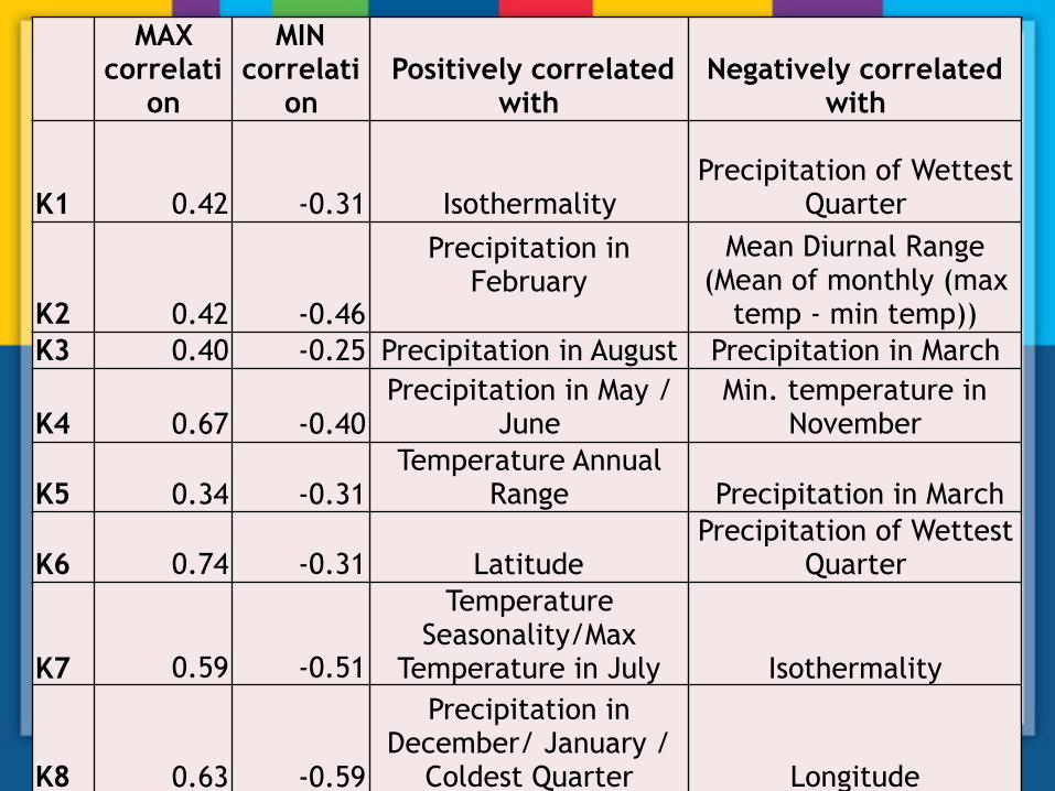
Some ancestral genomes may be adapted to local bio-climatic variables

We looked for putative association with the 19 bio-climatic variables, as defined by WorldClim (http://www.worldclim.org).

The “South Tunisian Coastal" genome is positively correlated to annual mean T°C (BIO1) and Mean T°C of colder quarter (BIO11) and negat ive ly cor re la ted to annua l precipitation (BIO12).

The “Spanish coastal" genome is

negatively correlated to T°C seasonality (BIO4), and T°C annual range (BIO7).

The “Greek" genome is positively correlated to precipitation of the wettest month (BIO13), precipitation seasonality (BIO15), precipitation of the wettest quarter (BIO16) and precipitation of coldest quarter (BIO19).

Spanish coastal

Greek

BIO1: r=0.26*** BIO11: r=-0.24** BIO12: r=--0.28***

BIO4: r=-0.42*** BIO7: r=-0.31***

BIO13: r=0.39*** BIO15: r=0.45*** BIO16: r=0.33*** BIO19: r=0.29***

The “North Tunisian Coastal" genome is not significantly correlated to any bioclimatic covariables.

Climate and geography explain less <50% of the variation in genome admixture component proportions

Other putative explanatory variables?

-soil structure and composition?

-Biotic interactions?


Verticillium sp. are soil-borne fungal pathogens for Legumes

V. alfalfae symptoms on susceptible M.truncatula

7 dpi

12 dpi

A17 (R) F83005.5 (S)

GFP -expressing V31-2 strain (Ben et al. 2013 ; Toueni et al. in preparation.)

Root pathogens enter the plant through root central cylinder

GFP Rs

GUS staining

Ralstonia solanacearum infection

xy

cwhy

* *

cor

xyhy

Verticillium albo-atrum infectionVailleau et al. 2006 Ben et al. 2012

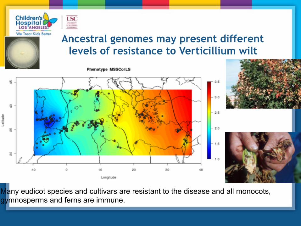
Ancestral genomes may present different levels of resistance to Verticillium wilt

Many eudicot species and cultivars are resistant to the disease and all monocots, gymnosperms and ferns are immune.

Ancestral genomes present different levels of resistance to Verticillium wilt

Linear Model (242 Mt HAPMAP accessions) MSSCorLS ~ K2 + K5 + K7 + K8

r²=0.31, P-value < 2.2 x 10-16

Can phenotype be predicted using GPS?

• Use plant model (Medicago truncatula) to test applicability of admixture framework to predict phenotypes.

• M. truncatula was infected with a fungal pathogen V. alfalfae

• MSS (Maximum symptom score) ranges from 0 (healthy) to 4 (dead), 2 threshold.

GPS was used to predict provenance of 59 unknown samples, and MSS was inferred based on the similarity of admixture profiles to the training set accessions Plants were infected in the lab and symptoms recorded 21/29 samples that are predicted to be resistant were resistant 24/30 samples predicted to be susceptible were susceptible

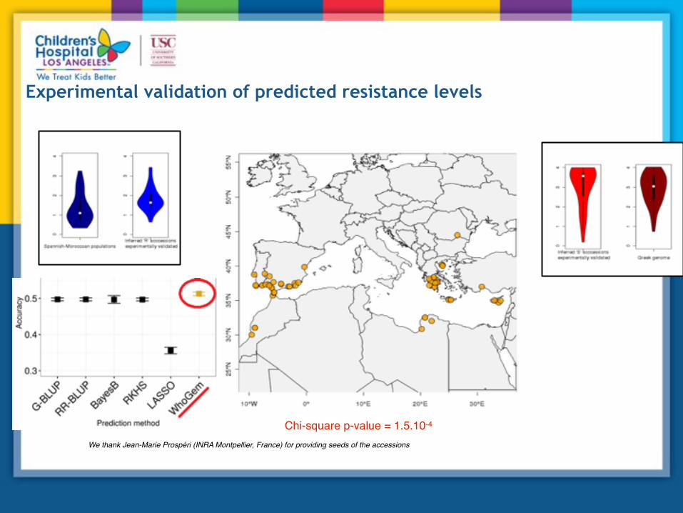
Experimental validation of predicted resistance levels

Chi-square p-value = 1.5.10-4

We thank Jean-Marie Prospéri (INRA Montpellier, France) for providing seeds of the accessions

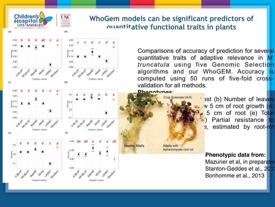
WhoGem models can be significant predictors of quantitative functional traits in plants

Phenotypic data from: Mazurier et al, in preparation Stanton-Geddes et al., 2013 Bonhomme et al., 2013Gentzbittel et al., pending submission

Comparisons of accuracy of prediction for several quantitative traits of adaptive relevance in M. truncatula using f ive Genomic Selection algorithms and our WhoGEM. Accuracy is computed using 50 runs of five-fold cross-validation for all methods. Phenotypes: (a) Plant height at harvest (b) Number of leaves (c) Nodule number below 5 cm of root growth (d) Nodule number above 5 cm of root (e) Total number of nodules (f) Partial resistance to Aphanomyces euteiches, estimated by root-rot index.

What is missing?Distance between two points should not be just geometric distance. Add: 1. Mode of propagation (e.g. Medicago seeds stick to goats) 2. Soil 3. Climate 4. Geography

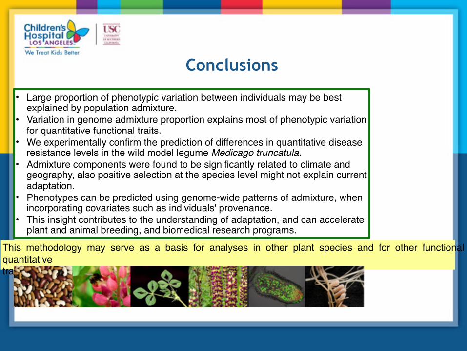
This methodology may serve as a basis for analyses in other plant species and for other functional quantitative traits of interest.

Conclusions

• Large proportion of phenotypic variation between individuals may be best explained by population admixture.

• Variation in genome admixture proportion explains most of phenotypic variation for quantitative functional traits.

• We experimentally confirm the prediction of differences in quantitative disease resistance levels in the wild model legume Medicago truncatula.

• Admixture components were found to be significantly related to climate and geography, also positive selection at the species level might not explain current adaptation.

• Phenotypes can be predicted using genome-wide patterns of admixture, when incorporating covariates such as individuals' provenance.

• This insight contributes to the understanding of adaptation, and can accelerate plant and animal breeding, and biomedical research programs.

MAX correlati

on

MIN correlati

on Positively correlated

withNegatively correlated

with

K1 0.42 -0.31 Isothermality Precipitation of Wettest

Quarter

K2 0.42 -0.46

Precipitation in February

Mean Diurnal Range (Mean of monthly (max

temp - min temp)) K3 0.40 -0.25 Precipitation in August Precipitation in March

K4 0.67 -0.40Precipitation in May /

June Min. temperature in

November

K5 0.34 -0.31Temperature Annual

Range Precipitation in March

K6 0.74 -0.31 LatitudePrecipitation of Wettest

Quarter

K7 0.59 -0.51

Temperature Seasonality/Max

Temperature in July Isothermality

K8 0.63 -0.59

Precipitation in December/ January /

Coldest Quarter Longitude

Soil/Climate

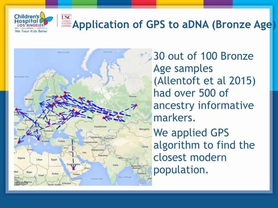
Application of GPS to aDNA (Bronze Age)

30 out of 100 Bronze Age samples (Allentoft et al 2015) had over 500 of ancestry informative markers. We applied GPS algorithm to find the closest modern population.

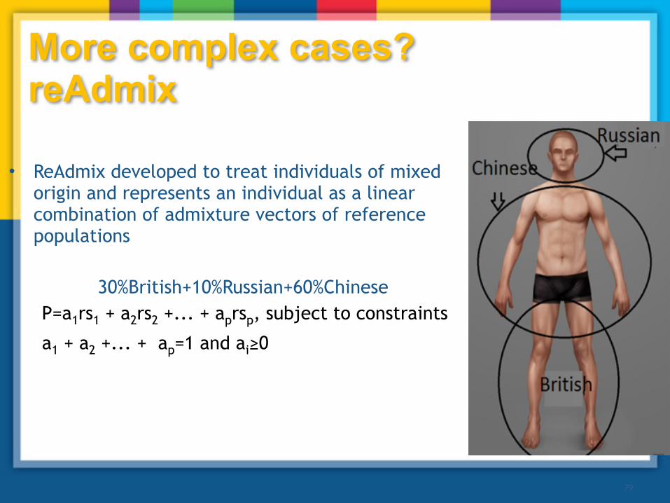
• ReAdmix developed to treat individuals of mixed origin and represents an individual as a linear combination of admixture vectors of reference populations

30%British+10%Russian+60%Chinese P=a1rs1 + a2rs2 +... + aprsp, subject to constraints

a1 + a2 +... + ap=1 and ai≥0

79

More complex cases? reAdmix

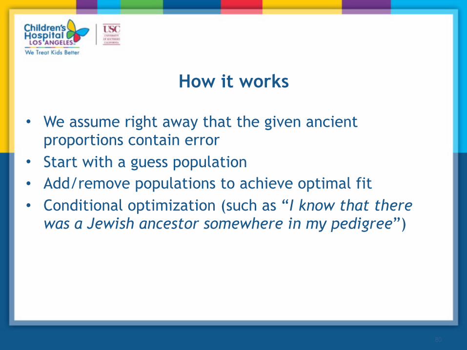
How it works

• We assume right away that the given ancient proportions contain error

• Start with a guess population • Add/remove populations to achieve optimal fit • Conditional optimization (such as “I know that there

was a Jewish ancestor somewhere in my pedigree”)

80

31.07.2017

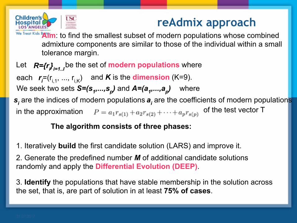
reAdmix approachAim: to find the smallest subset of modern populations whose combined admixture components are similar to those of the individual within a small tolerance margin.

The algorithm consists of three phases:

1. Iteratively build the first candidate solution (LARS) and improve it.2. Generate the predefined number M of additional candidate solutions randomly and apply the Differential Evolution (DEEP).

3. Identify the populations that have stable membership in the solution across the set, that is, are part of solution in at least 75% of cases.

Let R={ri}i=1..I be the set of modern populations where

ri=(ri,1, ..., ri,K) and K is the dimension (K=9).We seek two sets S=(s1,...,sp) and A=(a1,...,ap) where

si are the indices of modern populations ai are the coefficients of modern populationsin the approximation

each

of the test vector T

31.07.2017

Phase 1. Build and improve the initial solution set

S - individual’s ancestry

T – test vector

N - desired size of the solution

R – the set of modern populations

dim(S) < N

j=arg max[F(rj,T)] S = S ∪ {j}

aj=max[α:α·rj<T+ε]×β T = T − ajrj S0 = (S \ si) U {rk}

S = S0

i=0..dim(S) k=0..dim(R)

f(S0,T) < f(S,T)Affinity score

minimizes the loss function

where

Find the population vector with the highest affinity score Append this population to the solution set. Calculate the weight of the population vector

For all populations x in the current solution and for all y outside the solution, replace x with y, if it reduces the error.

31.07.2017

Phase 2. Optimize the solution by global stochastic and local search

2. Local search over all populations close to the preliminary solution

This step selects between related populations (e.g. Belorussian, Russian, and Ukrainian) that could have been misplaced in previous steps

S1,S2,...,SM

are generated randomly or from population groups

Objective function

is the approximation of Twhere

1. Differential Evolution Gmax number of iterations

DE: optimization method used for multidimensional real valued functions. Good for Treatment of noisy problems (Storn and Price, 1997)

31.07.2017

Phase 3. Averaging

S1:(a1,r1)1,(a2,r2)1,..,(ap-1,rp-1)1,(ap,rp)1

S2:(a1,r1)2,(a2,r2)2,..,(ap-1,rp-1)2,(ap,rp)2

SM:(a1,r1)M,(a2,r2)M,..,(ap-1,rp-1)M,(ap,rp)M

...

r belongs to final solution if: r=r1,1=r2,M-1=...=rp,M — is the same modern population

and

is present in L > 75% solutions

and

a=(1/L)(a1,1+a2,M-1+..+ap,M)

Reliable estimate: - the populations that are part of solution in at least 75% of cases,

- their averaged estimates of admixture proportion.

SM-1:(a1,r1)M-1,(a2,r2)M-1,..,(ap-1,rp-1)M-1,(ap,rp)M-1

S1, S2, ... , SM-1, SM — the set of candidate solutions. Final solution:

S=(s1,...,sp)A=(a1,...,ap)

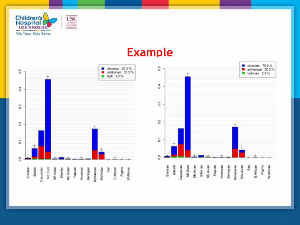
Example

85

Benchmark-1

Take sample that were validated by GPS1

Then we used ReAdmix in (a) unconditional and (b) conditional with incorrect guess mode.

(a) 94% of the samples were mapped to their reported ethnic group, and average distance to the correct location was 54±13 miles.

(b) with randomly chosen incorrect guess, 92% of samples was mapped to the reported ethnic group, with average distance to the correct location equal to 65±17 miles.

In all cases ReAdmix correctly identified the cases as un-mixed

86

Benchmark-2: simulated 500 50:50 mixtures

87

Testing mode Percent of at least one correctly predicted

origin

Percent of completely

correct predictions

Average distance to correct population, miles

Unconditional 78% 56% 324±46

Conditional on the equal weights, populations unknown

91% 74% 176±33

Conditional on one of the populations, weights unknown

NA 71% 104±16

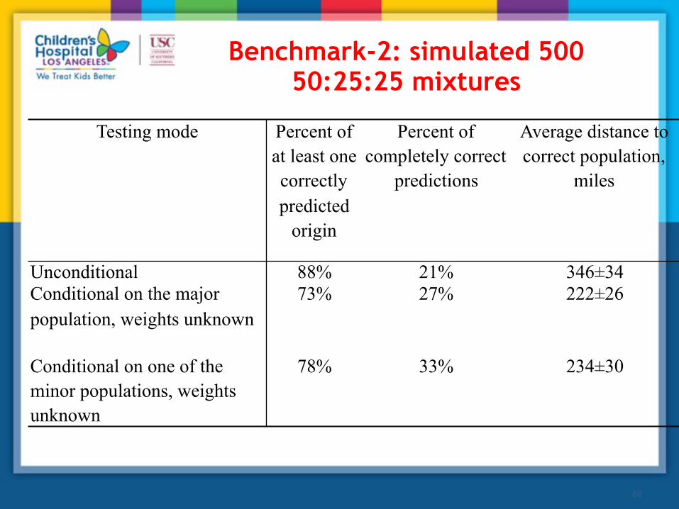
Benchmark-2: simulated 500 50:25:25 mixtures

88

Testing mode Percent of at least one correctly predicted

origin

Percent of completely correct

predictions

Average distance to correct population,

miles

Unconditional 88% 21% 346±34Conditional on the major population, weights unknown

73% 27% 222±26

Conditional on one of the minor populations, weights unknown

78% 33% 234±30

Sohn et (2012) al benchmark• 2 components • 4 components

4-dim space: European, African, Native American and East Asian

Color coding: red-European, green-African, yellow- Native American, blue-East Asian, and white- unassigned

Let’s practice!

Prediction of Functional Quantitative Traits in Plants...

Documents

Transcript of Prediction of Functional Quantitative Traits in Plants...