Prediction, Goodness-of-Fit, and Modeling Issues ECON 6002 Econometrics Memorial University of...

ECON 6002Econometrics Memorial University of Newfoundland

Adapted from Vera Tabakova’s notes

4.1 Least Squares Prediction

4.2 Measuring Goodness-of-Fit

4.3 Modeling Issues

4.4 Log-Linear Models

where e0 is a random error. We assume that and

. We also assume that and

0 1 2 0 0β βy x e

0 1 2 0E y x

0 0E e 20var e

0cov , 0 1,2, ,ie e i N

0 1 2 0y b b x

Figure 4.1 A point prediction

Slide 4-4Principles of Econometrics, 3rd Edition

0 0 1 2 0 0 1 2 0ˆf y y x e b b x

22 0

2

( )1var( ) 1

( )i

x xf

N x x

1 2 0 0 1 2 0

1 2 0 1 2 00 0

E f x E e E b E b x

x x

The variance of the forecast error is smaller when

i. the overall uncertainty in the model is smaller, as measured by the variance of the random errors ;

ii. the sample size N is larger;

iii. the variation in the explanatory variable is larger; and

iv. the value of the square deviation of our predicted point from the mean of X is small, predictions far away from the mean will be more imprecise.

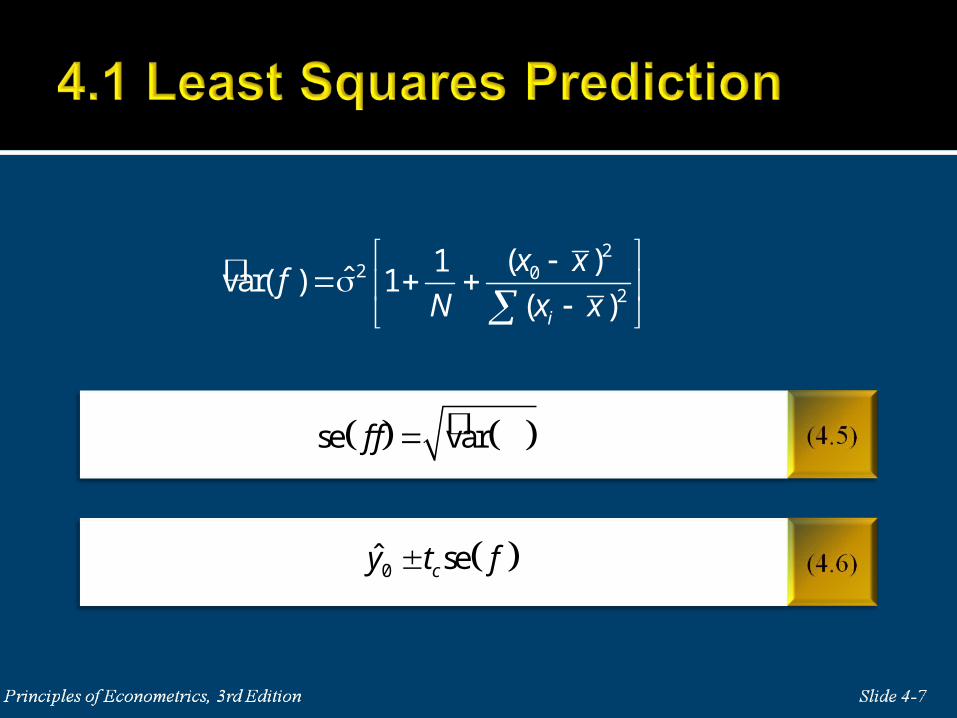
se varf f

0ˆ secy t f

2

2 02

( )1ˆvar( ) 1

( )i

x xf

N x x

Figure 4.2 Point and interval prediction


y

0 1 2 0ˆ 83.4160 10.2096(20) 287.6089y b b x

22 0

2

2 22 2

0 2

22 2

0 2

( )1ˆvar( ) 1

( )

ˆ ˆˆ ( )

( )

ˆˆ ( ) var

i

i

x xf

N x x

x xN x x

x x bN

0ˆ se( ) 287.6069 2.0244(90.6328) 104.1323,471.0854cy t f

1 2 i i iy x e

( )i i iy E y e

ˆ ˆi i iy y e

ˆ ˆ( )i i iy y y y e

Figure 4.3 Explained and unexplained components of yi


2 2 2ˆ ˆ( ) ( )i i iy y y y e

2

2ˆ1

iy

y y

N

= total sum of squares = SST: a measure of total variation in y about the sample mean.

= sum of squares due to the regression = SSR: that part of total variation in y, about the sample mean, that is explained by, or due to, the regression. Also known as the “explained sum of squares.”

= sum of squares due to error = SSE: that part of total variation in y about its mean that is not explained by the regression. Also known as the unexplained sum of squares, the residual sum of squares, or the sum of squared errors.

SST = SSR + SSE

2( )iy y

2ˆ( ) iy y

2ˆ ie

The closer R2 is to one, the closer the sample values yi are to the fitted regression

equation . If R2= 1, then all the sample data fall exactly on the fitted

least squares line, so SSE = 0, and the model fits the data “perfectly.” If the sample

data for y and x are uncorrelated and show no linear association, then the least

squares fitted line is “horizontal,” so that SSR = 0 and R2 = 0.

2 1SSR SSE

RSST SST

1 2ˆi iy b b x

cov( , )

var( ) var( )xy

xyx y

x y

x y

ˆ

ˆ ˆxy

xyx y

r

2

2

ˆ ( )( ) 1

ˆ ( ) 1

ˆ ( ) 1

xy i i

x i

y i

x x y y N

x x N

y y N

R2 measures the linear association, or goodness-of-fit, between the sample data

and their predicted values. Consequently R2 is sometimes called a measure of

“goodness-of-fit.”

2 2xyr R

2 2ˆyyR r

2

2 2

495132.160

ˆ ˆ 304505.176

i

i i i

SST y y

SSE y y e

2 304505.1761 1 .385

495132.160

SSER

SST

ˆ 478.75

.62ˆ ˆ 6.848 112.675

xyxy

x y

r

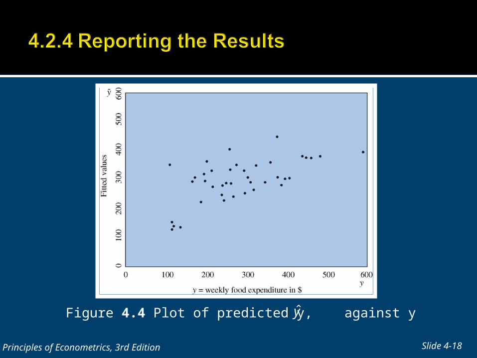
Figure 4.4 Plot of predicted y, against y


y

FOOD_EXP = weekly food expenditure by a household of size 3, in dollars

INCOME = weekly household income, in $100 units

* indicates significant at the 10% level

** indicates significant at the 5% level

*** indicates significant at the 1% level

2

* ***

83.42 10.21 .385

(se) (43.41) (2.09)

FOOD_EXP = INCOME R

4.3.1 The Effects of Scaling the Data Changing the scale of x:

Changing the scale of y:

* *1 2 1 2 1 2 = ( )( / ) = y x e c x c e x e

* *2 2where β β and c x x c

* * * *1 2 1 2/ ( / ) ( / ) ( / ) or y c c c x e c y x e

Variable transformations: Power: if x is a variable then xp means raising the variable to the power p; examples

are quadratic (x2) and cubic (x3) transformations.

The natural logarithm: if x is a variable then its natural logarithm is ln(x).

The reciprocal: if x is a variable then its reciprocal is 1/x.

Figure 4.5 A nonlinear relationship between food expenditure and income


The log-log model

The parameter β is the elasticity of y with respect to x.

The log-linear model

A one-unit increase in x leads to (approximately) a 100×β2 percent change in y.

The linear-log model

A 1% increase in x leads to a β2/100 unit change in y.

1 2ln( ) ln( )y x

1 2ln( )i iy x

2

1 2 ln or 100 100

yy x

x x

The reciprocal model is

The linear-log model is

1 2

1_FOOD EXP e

INCOME

1 2_ ln( )FOOD EXP INCOME e

Remark: Given this array of models, that involve different transformations of the dependent and independent variables, and some of which have similar shapes, what are some guidelines for choosing a functional form?

1.Choose a shape that is consistent with what economic theory tells us about the relationship.2.Choose a shape that is sufficiently flexible to “fit” the data3.Choose a shape so that assumptions SR1-SR6 are satisfied, ensuring that the least squares estimators have the desirable properties described in Chapters 2 and 3.

Figure 4.6 EViews output: residuals histogram and summary statistics for food expenditure example


The Jarque-Bera statistic is given by

where N is the sample size, S is skewness, and K is kurtosis.

In the food expenditure example

2

2 3

6 4

KNJB S

2

2 2.99 340.097 .063

6 4JB

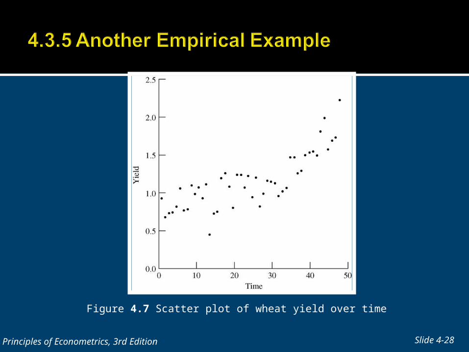
Figure 4.7 Scatter plot of wheat yield over time


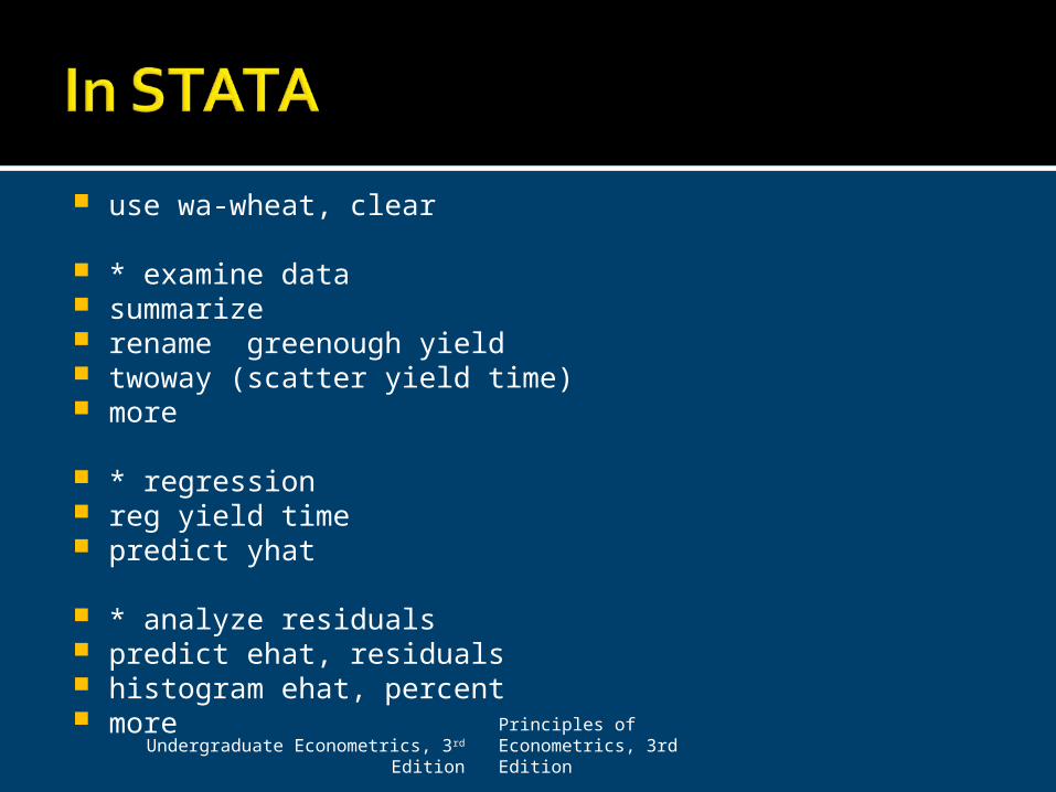
use wa-wheat, clear

* examine data summarize rename greenough yield twoway (scatter yield time) more

* regression reg yield time predict yhat

* analyze residuals predict ehat, residuals histogram ehat, percent more

Undergraduate Econometrics, 3rd Edition

Principles of Econometrics, 3rd Edition

twoway (scatter yield time) (connect yhat time) more twoway (scatter yield time) (lfit yield time) more twoway connected ehat time, yline(0) more rvpplot time, recast(bar) yline(0) more

Undergraduate Econometrics, 3rd Edition

Principles of Econometrics, 3rd Edition

1 2t t tYIELD TIME e

2.638 .0210 .649

(se) (.064) (.0022)t tYIELD TIME R

Figure 4.8 Predicted, actual and residual values from straight line


Figure 4.9 Bar chart of residuals from straight line


31 2t t tYIELD TIME e

20.874 9.68 0.751

(se) (.036) (.082)t tYIELD TIMECUBE R

3 1000000TIMECUBE TIME

Figure 4.10 Fitted, actual and residual values from equation with cubic term


4.4.1 The Growth Model

0

1 2

ln ln ln 1tYIELD YIELD g t

t

ln .3434 .0178

(se) (.0584) (.0021) tYIELD t

4.4.2 A Wage Equation

0

1 2

ln ln ln 1WAGE WAGE r EDUC

EDUC

ln .7884 .1038

(se) (.0849) (.0063)

WAGE EDUC

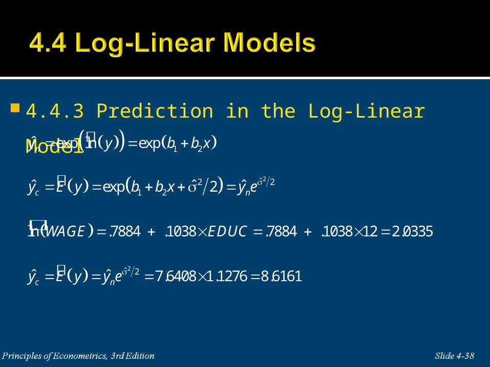
4.4.3 Prediction in the Log-Linear Model

1 2ˆ exp ln expny y b b x

2ˆ2 21 2ˆ ˆ ˆexp 2c ny E y b b x y e

ln .7884 .1038 .7884 .1038 12 2.0335WAGE EDUC

2ˆ 2ˆ ˆ 7.6408 1.1276 8.6161c ny E y y e

4.4.4 A Generalized R2 Measure

R2 values tend to be small with microeconomic, cross-sectional data, because the

variations in individual behavior are difficult to fully explain.

22 2ˆ,ˆcorr ,g y yR y y r

22 2ˆcorr , .4739 .2246g cR y y

4.4.5 Prediction Intervals in the Log-Linear Model

exp ln se ,exp ln sec cy t f y t f

exp 2.0335 1.96 .4905 ,exp 2.0335 1.96 .4905 2.9184,20.0046

41Principles of Econometrics, 3rd Edition


0 0 1 2 0 0 1 2 0ˆf y y x e b b x

20 1 2 0 1 0 2 0 1 2

2 2 22 20 02 2 2

ˆvar var var var 2 cov ,

2i

i i i

y b b x b x b x b b

x xx x

N x x x x x x


22 2 2 2 2 2 2 200

0 2 2 2 2 2

2 2 2 22 0 0

2 2

2 2

2 02 2

2

2 0

2ˆvar

2

1

i

i i i i i

i

i i

i

i i

x xx Nx x Nxy

N x x N x x x x x x N x x

x Nx x x x x

N x x x x

x x x x

N x x x x

x x

N x

2

i x


(4A.1)

(4A.2)

~ (0,1)var( )

fN

f

2

2 02

1 ( )ˆvar 1

( )i

x xf

N x x

0 0

( 2)

ˆ~

se( )varN

f y yt

ff

( ) 1c cP t t t


0 0ˆ[ ] 1

se( )c c

y yP t t

f

0 0 0ˆ ˆse( ) se( ) 1c cP y t f y y t f


22 2 2ˆ ˆ ˆ ˆ ˆ ˆ( ) ( ) 2( )i i i i i i iy y y y e y y e y y e

2 2 2ˆ ˆ ˆ ˆ( ) 2 ( )i i i i iy y y y e y y e

1 2

1 2

ˆ ˆ ˆ ˆ ˆ ˆ ˆ

ˆ ˆ ˆ

i i i i i i i i

i i i i

y y e y e y e b b x e y e

b e b x e y e


If the model contains an intercept it is guaranteed that SST = SSR + SSE. If, however, the model does not contain an intercept, then and SST ≠ SSR + SSE.

1 2 1 2ˆ 0i i i i ie y b b x y Nb b x

21 2 1 2ˆ 0i i i i i i i i ix e x y b b x x y b x b x

ˆ ˆ 0i iy y e

ˆ 0ie

Suppose that the variable y has a normal distribution, with mean μ and variance σ2. If we consider then is said to have a log-normal distribution.


yw e 2ln ~ ,y w N

2 2E w e

2 22var 1w e e

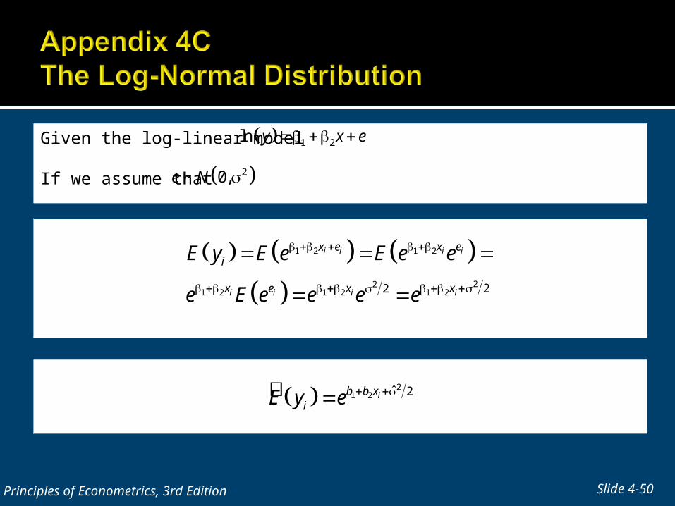
Given the log-linear model

If we assume that


1 2ln y x e

2~ 0,e N

1 2 1 2

221 2 1 2 1 2 22

i i i i

i i i i

x e x ei

x e x x

E y E e E e e

e E e e e e

21 2 ˆ 2ib b x

iE y e

The growth and wage equations:

and


2 ln 1 r 2 1r e

222 2 2~ ,var ib N b x x

2 22 var /2bbE e e

2 2var /2ˆ 1b br e

222 ˆvar ib x x

Prediction, Goodness-of-Fit, and Modeling Issues ECON 6002 Econometrics Memorial University of...

Documents

Transcript of Prediction, Goodness-of-Fit, and Modeling Issues ECON 6002 Econometrics Memorial University of...