PREDICTING CHANGES TO SOURCE CODE A Thesis presented …...Organizations typically use issue...
115
PREDICTING CHANGES TO SOURCE CODE A Thesis presented to the Faculty of California Polytechnic State University, San Luis Obispo In Partial Fulfillment of the Requirements for the Degree Master of Science in Computer Science by Justin Roll April 2016
Transcript of PREDICTING CHANGES TO SOURCE CODE A Thesis presented …...Organizations typically use issue...

PREDICTING CHANGES TO SOURCE CODE
A Thesis
presented to
the Faculty of California Polytechnic State University,
San Luis Obispo
In Partial Fulfillment
of the Requirements for the Degree
Master of Science in Computer Science
by
Justin Roll
April 2016

c© 2016
Justin Roll
ALL RIGHTS RESERVED
ii

COMMITTEE MEMBERSHIP
TITLE: Predicting Changes to Source Code
AUTHOR: Justin Roll
DATE SUBMITTED: April 2016
COMMITTEE CHAIR: Davide Falessi, Ph.D.
Associate Professor of Computer Science
COMMITTEE MEMBER: Foaad Khosmood, Ph.D.
Assistant Professor of Computer Science
COMMITTEE MEMBER: Alexander Dekhytar, Ph.D.
Professor of Computer Science
iii

ABSTRACT
Predicting Changes to Source Code
Justin Roll
Organizations typically use issue tracking systems (ITS) such as Jira to plan soft-
ware releases and assign requirements to developers. Organizations typically also use
source control management (SCM) repositories such as Git to track historical changes
to a code-base. These ITS and SCM repositories contain valuable data that remains
largely untapped. As developers churn through an organization, it becomes expensive
for developers to spend time determining which software artifact must be modified
to implement a requirement. In this work we created, developed, tested and evalu-
ated a tool called Class Change Predictor, otherwise known as CCP, for predicting
which class will implement a requirement. Understanding which class will implement
a requirement supports several software engineering tasks such as refactoring and
assigning requirements to developers.
CCP is a data-mining tool operating on top of ITS and SCM repositories which
gathers a unique combination of metrics. CCP leverages requirement text to compare
current requirements to past requirements and requirements to source code files. CCP
performs static analysis on the code-base of each major release of the software artifact.
We evaluated CCP on different open source datasets (and the Digital Democracy
dataset) by using several machine learning classifiers and pre-processing procedures.
Our results show that we can achieve high precision on three out of four datasets. We
conclude that accurate class change prediction is feasible, and we propose numerous
solutions to increase future accuracy.
iv

ACKNOWLEDGMENTS
Thanks to:
• Dr. Davide Falessi, for so much direction and patience.
• Jin Guo from DePaul University, for coding all of the similarity metrics and
providing me numerous papers on their meaning.
• Dr. Jane Cleland-Huang from DePaul University, for wisdom and guidance.
• Dr. Alexander Dekhtyar, for letting a humble former humanities major like
myself into this program.
• Dr. Foaad Khosmood, for getting me interested in machine learning.
• Nicole L. Smith, for love and support.
• Mom and Dad, just because.
v

TABLE OF CONTENTS
Page
LIST OF TABLES . . . . . . . . . . . . . . . . . . . . . . . . . . . . . . . . . xii
LIST OF FIGURES . . . . . . . . . . . . . . . . . . . . . . . . . . . . . . . . xiii
CHAPTER
1 Introduction . . . . . . . . . . . . . . . . . . . . . . . . . . . . . . . . . . . 1
1.1 An Overview . . . . . . . . . . . . . . . . . . . . . . . . . . . . . . . 1
1.1.1 Impact . . . . . . . . . . . . . . . . . . . . . . . . . . . . . . . 2
1.2 Research Questions . . . . . . . . . . . . . . . . . . . . . . . . . . . . 3
1.2.1 RQ1: What Is The Most Accurate Configuration For The CCPSystem? . . . . . . . . . . . . . . . . . . . . . . . . . . . . . . 3
1.2.1.1 Conjecture . . . . . . . . . . . . . . . . . . . . . . . 3
1.2.1.2 Hypothesis . . . . . . . . . . . . . . . . . . . . . . . 3
1.2.2 RQ2: What Is The Overall Accuracy Of Our Classifier On EachDataset? . . . . . . . . . . . . . . . . . . . . . . . . . . . . . . 3
1.2.2.1 Conjecture . . . . . . . . . . . . . . . . . . . . . . . 4
1.2.2.2 Hypothesis . . . . . . . . . . . . . . . . . . . . . . . 4
1.2.3 RQ3: How Does The CCP Classifier Compare To Other SimilarStudies? . . . . . . . . . . . . . . . . . . . . . . . . . . . . . . 4
1.2.3.1 Conjecture . . . . . . . . . . . . . . . . . . . . . . . 4
1.2.3.2 Hypothesis . . . . . . . . . . . . . . . . . . . . . . . 4
2 Background and Related Work . . . . . . . . . . . . . . . . . . . . . . . . 5
2.1 Background . . . . . . . . . . . . . . . . . . . . . . . . . . . . . . . . 5
2.1.1 Static Analysis . . . . . . . . . . . . . . . . . . . . . . . . . . 5
2.1.2 Object-oriented Complexity . . . . . . . . . . . . . . . . . . . 5
2.1.3 Natural Language Processing Techniques . . . . . . . . . . . . 6
2.1.3.1 Pre-processing . . . . . . . . . . . . . . . . . . . . . 6
2.1.3.2 Vector Space Model . . . . . . . . . . . . . . . . . . 6
2.1.3.3 Document Similarity . . . . . . . . . . . . . . . . . . 7
2.2 Classification . . . . . . . . . . . . . . . . . . . . . . . . . . . . . . . 9
2.2.1 Supervised Machine Learning . . . . . . . . . . . . . . . . . . 10
vi

2.3 Related Work . . . . . . . . . . . . . . . . . . . . . . . . . . . . . . . 10
2.3.1 Source Code Traceability . . . . . . . . . . . . . . . . . . . . . 10
2.3.1.1 Event-based Traceability . . . . . . . . . . . . . . . . 10
2.3.1.2 Traceability With Machine Learning Classifiers . . . 11
2.3.1.3 Relation To Our Project . . . . . . . . . . . . . . . . 12
2.3.2 Impact Analysis . . . . . . . . . . . . . . . . . . . . . . . . . . 12
2.3.3 Manual Impact Analysis . . . . . . . . . . . . . . . . . . . . . 13
2.3.4 Automated Impact Analysis . . . . . . . . . . . . . . . . . . . 14
2.3.4.1 Predicting Class Changes Using Co-change History . 15
2.3.4.2 Predicting Software Changes From Requirements . . 16
2.3.5 Relation To Our Project . . . . . . . . . . . . . . . . . . . . . 17
3 Approach . . . . . . . . . . . . . . . . . . . . . . . . . . . . . . . . . . . . 18
3.1 Linking Process . . . . . . . . . . . . . . . . . . . . . . . . . . . . . . 18
3.1.1 From RequirementId To Commit . . . . . . . . . . . . . . . . 19
3.1.2 Determining Touched And Untouched Classes For Each Re-quirement . . . . . . . . . . . . . . . . . . . . . . . . . . . . . 21
3.1.3 Determining Releases . . . . . . . . . . . . . . . . . . . . . . . 22
3.2 Natural Language Processing . . . . . . . . . . . . . . . . . . . . . . 23
3.2.1 Pre-processing . . . . . . . . . . . . . . . . . . . . . . . . . . . 23
3.2.2 Requirement Similarity . . . . . . . . . . . . . . . . . . . . . . 24
3.3 Temporal Locality Calculation . . . . . . . . . . . . . . . . . . . . . . 28
3.3.1 Simple Modification % . . . . . . . . . . . . . . . . . . . . . . 28
3.3.2 Linear Temporal Locality Modification Score . . . . . . . . . . 29
3.3.3 Logarithmic Temporal Locality Modification Score . . . . . . . 29
3.3.4 Example Calculations . . . . . . . . . . . . . . . . . . . . . . . 30
3.4 ML Classifier . . . . . . . . . . . . . . . . . . . . . . . . . . . . . . . 32
3.4.1 Feature Pre-processing Configurations . . . . . . . . . . . . . 33
3.4.1.1 Principal Component Analysis . . . . . . . . . . . . 33
3.4.1.2 Top 5 Information Gain . . . . . . . . . . . . . . . . 34
3.4.2 Classifiers . . . . . . . . . . . . . . . . . . . . . . . . . . . . . 34
3.4.2.1 Naive Bayes . . . . . . . . . . . . . . . . . . . . . . . 34
3.4.2.2 Bootstrap Aggregation . . . . . . . . . . . . . . . . . 35
vii

3.4.2.3 Decision Tree . . . . . . . . . . . . . . . . . . . . . . 36
3.4.2.4 The J48 Decision Tree . . . . . . . . . . . . . . . . . 36
3.4.2.5 Random Forest . . . . . . . . . . . . . . . . . . . . . 37
3.4.3 Cross-Validation . . . . . . . . . . . . . . . . . . . . . . . . . 37
4 Class Change Predictor . . . . . . . . . . . . . . . . . . . . . . . . . . . . . 38
4.1 Data Stores . . . . . . . . . . . . . . . . . . . . . . . . . . . . . . . . 38
4.1.1 Jira . . . . . . . . . . . . . . . . . . . . . . . . . . . . . . . . 38
4.1.1.1 Jira Extractor . . . . . . . . . . . . . . . . . . . . . . 40
4.1.1.2 Parsing Jira Data Into Requirements . . . . . . . . . 40
4.1.2 Git . . . . . . . . . . . . . . . . . . . . . . . . . . . . . . . . . 41
4.1.3 JGit . . . . . . . . . . . . . . . . . . . . . . . . . . . . . . . . 42
4.1.3.1 Git Extractor . . . . . . . . . . . . . . . . . . . . . . 42
4.2 Build Tools . . . . . . . . . . . . . . . . . . . . . . . . . . . . . . . . 42
4.2.1 Maven . . . . . . . . . . . . . . . . . . . . . . . . . . . . . . . 43
4.3 Release Metrics Storage And Tools . . . . . . . . . . . . . . . . . . . 43
4.3.1 SonarQube . . . . . . . . . . . . . . . . . . . . . . . . . . . . 45
4.3.1.1 SonarQube Executor . . . . . . . . . . . . . . . . . . 46
4.3.1.2 SonarQube Scraper . . . . . . . . . . . . . . . . . . . 46
4.3.2 CKJM Extractor . . . . . . . . . . . . . . . . . . . . . . . . . 47
4.4 Other Technologies . . . . . . . . . . . . . . . . . . . . . . . . . . . . 47
4.4.1 The Semantic Similarity Toolkit . . . . . . . . . . . . . . . . . 47
4.4.2 Weka . . . . . . . . . . . . . . . . . . . . . . . . . . . . . . . . 48
4.4.2.1 Attribute-Relation File Format . . . . . . . . . . . . 48
4.5 Configuration And Operation . . . . . . . . . . . . . . . . . . . . . . 48
4.5.1 Configuration . . . . . . . . . . . . . . . . . . . . . . . . . . . 49
4.5.2 Commandline Operation . . . . . . . . . . . . . . . . . . . . . 49
4.6 Overall Process . . . . . . . . . . . . . . . . . . . . . . . . . . . . . . 51
4.6.1 Operation Scenarios . . . . . . . . . . . . . . . . . . . . . . . 52
4.6.1.1 Scenario 1: Compute And Serialize Requirements . . 52
4.6.1.2 Scenario 2: Analyze Releases . . . . . . . . . . . . . 53
4.6.1.3 Scenario 3: Prepare ARFF Files . . . . . . . . . . . 53
4.6.1.4 Scenario 4: Ensemble . . . . . . . . . . . . . . . . . . 53
viii

5 Evaluation . . . . . . . . . . . . . . . . . . . . . . . . . . . . . . . . . . . . 55
5.1 Variables . . . . . . . . . . . . . . . . . . . . . . . . . . . . . . . . . . 55
5.1.1 Dependent . . . . . . . . . . . . . . . . . . . . . . . . . . . . . 55
5.1.1.1 Precision . . . . . . . . . . . . . . . . . . . . . . . . 55
5.1.1.2 Recall . . . . . . . . . . . . . . . . . . . . . . . . . . 56
5.1.1.3 F 0.1 Score . . . . . . . . . . . . . . . . . . . . . . . 56
5.1.2 Independent . . . . . . . . . . . . . . . . . . . . . . . . . . . . 57
5.1.2.1 SonarQube Violations . . . . . . . . . . . . . . . . . 57
5.1.2.2 SonarQube Code Complexity . . . . . . . . . . . . . 57
5.1.2.3 Lines Of Code . . . . . . . . . . . . . . . . . . . . . 58
5.1.2.4 Change Frequency . . . . . . . . . . . . . . . . . . . 58
5.1.2.5 Linear Temporal Locality . . . . . . . . . . . . . . . 58
5.1.3 Logarithmic Temporal Locality . . . . . . . . . . . . . . . . . 58
5.1.3.1 CKJM WMC: Weighted Methods Per Class . . . . . 59
5.1.3.2 CKJM DIT: Depth Of Inheritance Tree . . . . . . . 59
5.1.3.3 CKJM NOC: Number Of Children . . . . . . . . . . 59
5.1.3.4 CKJM CBO: Coupling Between Object Classes . . . 59
5.1.3.5 CKJM RFC: Response For A Class . . . . . . . . . . 60
5.1.3.6 CKJM LCOM: Lack Of Cohesion In Methods . . . . 60
5.1.3.7 CKJM Ca: Afferent Couplings . . . . . . . . . . . . 60
5.1.3.8 CKJM NPM: Number Of Public Methods . . . . . . 61
5.2 Projects . . . . . . . . . . . . . . . . . . . . . . . . . . . . . . . . . . 61
5.2.1 Selected Projects . . . . . . . . . . . . . . . . . . . . . . . . . 62
5.2.1.1 Apache Tika . . . . . . . . . . . . . . . . . . . . . . 62
5.2.1.2 Apache Isis . . . . . . . . . . . . . . . . . . . . . . . 63
5.2.1.3 Apache Accumulo . . . . . . . . . . . . . . . . . . . 63
5.2.1.4 Digital Democracy . . . . . . . . . . . . . . . . . . . 63
5.3 Results . . . . . . . . . . . . . . . . . . . . . . . . . . . . . . . . . . . 63
5.3.1 RQ1: What Is The Best Configuration Of Our Approach? . . 64
5.3.1.1 Best Configuration . . . . . . . . . . . . . . . . . . . 65
5.3.1.2 Best Pre-processing Configuration . . . . . . . . . . 65
5.3.1.3 Best Classifier Configuration . . . . . . . . . . . . . 67
ix

5.4 RQ2: What Was The Overall Accuracy Of Our Approach? . . . . . . 67
5.5 RQ3: How Does Our Model Compare To Others? . . . . . . . . . . . 69
5.5.1 Comparison To Random Approach . . . . . . . . . . . . . . . 69
5.5.2 Comparison To Previous Studies . . . . . . . . . . . . . . . . 70
5.5.3 Analysis . . . . . . . . . . . . . . . . . . . . . . . . . . . . . . 70
6 Conclusion And Future Work . . . . . . . . . . . . . . . . . . . . . . . . . 73
6.1 Threats To Validity . . . . . . . . . . . . . . . . . . . . . . . . . . . . 74
6.2 Future Work . . . . . . . . . . . . . . . . . . . . . . . . . . . . . . . . 74
6.2.1 Deeper Analysis Of The Results . . . . . . . . . . . . . . . . . 75
6.2.1.1 Compare The Accuracy Of Estimates Made By UsingA Single Set Of Metrics Versus The Complete Set . . 75
6.2.1.2 Compare The Accuracy Of Estimates Made By UsingSingle Metrics Versus The Complete Set Of Metrics . 75
6.2.1.3 Compare The Accuracy Of Our Approach When Us-ing Only Data Related To The First Requirement Ver-sus The Entire Dataset . . . . . . . . . . . . . . . . . 75
6.2.1.4 Find Better Temporal Locality Scores . . . . . . . . 76
6.2.1.5 Analyze The Locality Of Changes In The DifferentDatasets . . . . . . . . . . . . . . . . . . . . . . . . . 76
6.2.1.6 Identify Other Dataset Characteristics Impacting TheAccuracy Of Our Estimates . . . . . . . . . . . . . . 77
6.2.2 Approach Improvements . . . . . . . . . . . . . . . . . . . . . 77
6.2.2.1 Leveraging Architecture Relations Information . . . . 77
6.2.2.2 Leveraging Co-changes Information . . . . . . . . . . 78
6.2.2.3 Pre-process The Requirements For Their Quality . . 78
6.2.2.4 Leveraging Interconnected Frequency Information: High-est Frequency Of A Connected Class . . . . . . . . . 79
6.2.2.5 Leveraging Interconnected Complexity Information . 79
6.2.2.6 Measuring All Metrics For Every Revision Rather ThanFor Every Release . . . . . . . . . . . . . . . . . . . 79
6.2.3 Raised Research Questions: Measuring The Usefulness Of OurApproach In Practice . . . . . . . . . . . . . . . . . . . . . . . 80
6.2.3.1 Release Planning: What is The Reduction Of DefectsProvided By Minimizing The Number Of DevelopersTouching The Same Class? . . . . . . . . . . . . . . 80
x

6.2.3.2 Refactoring: How Many Refactoring Decisions CouldBe Avoided Or Improved By Using Our Approach? . 81
6.2.3.3 Effort Estimation: What Is The Improved AccuracyOf Effort Estimation Provided By Our Approach? . . 81
6.2.3.4 Defect Estimation: What Is The Improved AccuracyOf Defects Estimation Provided By Our Approach? . 82
6.3 Final Thoughts . . . . . . . . . . . . . . . . . . . . . . . . . . . . . . 82
BIBLIOGRAPHY . . . . . . . . . . . . . . . . . . . . . . . . . . . . . . . . . 83
APPENDICES
A Example Class Change . . . . . . . . . . . . . . . . . . . . . . . . . . 91
B XML Configuration Example . . . . . . . . . . . . . . . . . . . . . . 94
C Weka Configuration . . . . . . . . . . . . . . . . . . . . . . . . . . . . 96
D Features . . . . . . . . . . . . . . . . . . . . . . . . . . . . . . . . . . 98
xi

LIST OF TABLES
Table Page
3.1 Example Of Temporal Locality Result For Three Classes . . . . . . 31
3.2 Temporal Locality Example . . . . . . . . . . . . . . . . . . . . . . 33
4.1 Configuration Options . . . . . . . . . . . . . . . . . . . . . . . . . 49
4.2 Command-line Flags . . . . . . . . . . . . . . . . . . . . . . . . . . 50
5.1 Statistics For The 4 Datasets . . . . . . . . . . . . . . . . . . . . . 62
5.2 Highest F0.5 Scores By Feature And Classifier . . . . . . . . . . . . 66
5.3 Accuracy Per Dataset . . . . . . . . . . . . . . . . . . . . . . . . . 68
C.1 Weka Parameters . . . . . . . . . . . . . . . . . . . . . . . . . . . . 97
D.1 Requirements To Code Metrics . . . . . . . . . . . . . . . . . . . . 99
D.2 Textual Similarity Methods To Compute Requirements To Class As-sociations . . . . . . . . . . . . . . . . . . . . . . . . . . . . . . . . 100
D.3 Temporal Locality Metrics . . . . . . . . . . . . . . . . . . . . . . . 101
D.4 Source Code Coupling, Cohesion, And Complexity Metrics . . . . . 102
xii

LIST OF FIGURES
Figure Page
3.1 Relationship Between Requirements And Commits . . . . . . . . . 19
3.2 Requirement And Commit Life Cycle . . . . . . . . . . . . . . . . . 22
3.3 Dataset Visual . . . . . . . . . . . . . . . . . . . . . . . . . . . . . 23
3.4 Requirement To Requirement Similarity Example . . . . . . . . . . 26
4.1 System Workflow . . . . . . . . . . . . . . . . . . . . . . . . . . . . 39
4.2 A Maven Dependency Graph . . . . . . . . . . . . . . . . . . . . . 44
4.3 How The System Snapshots Releases . . . . . . . . . . . . . . . . . 45
4.4 Map Of Metric Storage Structure . . . . . . . . . . . . . . . . . . . 45
5.1 Configuration Comparison . . . . . . . . . . . . . . . . . . . . . . . 65
5.2 Configuration Table . . . . . . . . . . . . . . . . . . . . . . . . . . 66
5.3 Evaluation Data Across All 4 Datasets . . . . . . . . . . . . . . . . 69
5.4 Comparison To Random . . . . . . . . . . . . . . . . . . . . . . . . 71
5.5 Comparison To Previous Studies . . . . . . . . . . . . . . . . . . . 72
A.1 First Modification . . . . . . . . . . . . . . . . . . . . . . . . . . . 91
A.2 Large Amount Of Modifications . . . . . . . . . . . . . . . . . . . . 92
A.3 Many IO-related Modifications . . . . . . . . . . . . . . . . . . . . 92
A.4 Final Modification . . . . . . . . . . . . . . . . . . . . . . . . . . . 93
xiii

Chapter 1
INTRODUCTION
1.1 An Overview
In the past quarter century, software has grown from a minor niche to an industry
worth hundreds of billions of dollars [65]. Complex software systems are relied upon
for every facet of business, and, for many people, software use is intertwined with
every-day life. People use software when they contact their friends on social media,
when finding directions to a near-by restaurant, and even when starting their car.
The high demand for software is exacerbated by the difficulty required in developing
complex software systems.
In addition to technical knowledge, software engineering, like other engineer-
ing disciplines, typically requires planning. In recent years, agile programming has
emerged as a popular software engineering methodology [35]. Under agile methodolo-
gies, software is developed piece by piece, using some type of issue-tracking system
such as Atlassian’s Jira to track development tasks[10]. Software Development Man-
agers, and sometimes the software developers themselves, write requirements which
must be implemented by the software, then post them on an issue tracking system.
Once a developer finishes making a code change, she commits it to a source control
management system for safe-keeping. Later in the project life-cycle, a thoroughly
completed series of software changes is then packaged into a release for public con-
sumption.
Even programmers possessing the technical knowledge required to work on a new
software project must often take time to obtain the proper domain knowledge of a
software system. A newly hired programmer often has to spend a great deal of time
1

pouring over design documentation, F.A.Q.s, and project wikis. If a programmer is
asked to make a certain change to a piece of software, the programmer often has to dive
into the organization’s project management software, finding previous requirements
and checking the code changes required to implement them.
Developers also have to make numerous decisions related to the refactoring of
software. Refactoring refers to the process of making non-functional changes to soft-
ware [55]. Refactoring often involves changes such as reducing the complexity of code,
making the code more readable, and making code more modular. Refactoring activi-
ties can often reduce the accumulated technical debt of a project, at the cost of some
lost immediate work [55].
1.1.1 Impact
Due to the trade-off of immediate vs. long-term costs, developers are often at a loss
as to when to perform a specific refactoring activity. If there is a high likelyhood
that a code fragment will change in the future, it can be assumed that there will be
benefits to refactoring, as presumably refactoring of the code would reduce the effort
required for future changes. However, if the code fragment is unlikely to be modified
in the future, it is less useful to refactor it in the present [55].
Developers who can accurately predict what software artifacts will be modified
as a result of a requirement are termed domain experts, and often spend valuable
development time training new hires. But what if this process could be automated?
If a system could be built that would immediately make a code change prediction
based on the text of a requirement and the state of the current code-base, this would
save organizations valuable time and money.
In response to this need, we introduce Class Change Predictor, or CCP. CCP
leverages textual requirement data to compare requirements to other requirements
2

and requirements to code. CCP records the state of the code-base as of each ma-
jor release of the software artifact. CCP then trains a machine learning classifier
using textual similarity measures, static analysis metrics, object-oriented complexity
metrics, and code change history.
1.2 Research Questions
In this study, we answer three main research questions. Listed below are the research
questions, our conjecture behind them, and our hypotheses.
1.2.1 RQ1: What Is The Most Accurate Configuration For The CCP System?
We attempt to maximize the accuracy of CCP by testing with multiple machine
learning classifiers and feature sets.
1.2.1.1 Conjecture
Data models often need tuning in order to reach peak accuracy. By testing CCP with
several different configurations, we are more likely to find the optimal model.
1.2.1.2 Hypothesis
CCP’s accuracy is significantly higher with an optimal feature configuration.
1.2.2 RQ2: What Is The Overall Accuracy Of Our Classifier On Each Dataset?
Thorough testing is paramount in generating a high-quality machine learning classi-
fier. Machine learning classifiers should be tested with metrics appropriate to domain
needs.
3

1.2.2.1 Conjecture
If the CCP tool falsely tells a developer that a class needs to be changed, the developer
wastes valuable time before realizing that the class does not need modification. When
building CCP, we prioritize accuracy measures that penalize false positives and reward
true positives.
1.2.2.2 Hypothesis
CCP is trained with features that are informative. CCP’s accuracy measures are high
on a variety of datasets.
1.2.3 RQ3: How Does The CCP Classifier Compare To Other Similar Studies?
We compare our classifier with multiple related systems in order to properly assess
performance.
1.2.3.1 Conjecture
In order for CCP to be useful in industry, it must provide results that are intelligent.
CCP must perform significantly better than a random classifier. To further gauge the
results, we compare CCP with previous studies on class change prediction.
1.2.3.2 Hypothesis
CCP’s accuracy metrics are significantly better than a random classifier overall. CCP
provides results that are competitive with prior studies.
4

Chapter 2
BACKGROUND AND RELATED WORK
2.1 Background
This section provides technical background on the various concepts related to the
creation of CCP. It also introduces concepts that are critical to understanding outside
research related to the CCP project.
2.1.1 Static Analysis
Static analysis in terms of software engineering refers to the process of analyzing
code without actually running it. There is significant evidence that static analysis is
effective in finding faults in software [73]. Developers often run static analysis utilities
such as FindBugs at every build iteration in order to find issues such as unused
variables, endless loops, and casting errors [7]. Organizations run static analysis tools
such as SonarQube at a larger scale, monitoring their entire code-base for quality [67].
2.1.2 Object-oriented Complexity
Software artifacts in object-oriented systems can have numerous dependencies. Classes
inherit data from their parent classes and are linked to by other classes. A class could
have ten lines of code, but many more dependencies. Thus, researchers Kidamberer
and Kemberer devised several object-oriented metrics designed to illustrate the com-
plexity and coupling of classes [27]. Classes with high scores in these metrics often
have ripple effects - modifying one of these classes can mean modifying several de-
pendent classes.
5

2.1.3 Natural Language Processing Techniques
Natural Language Processing is the study of the synthesis between computer and
human language [19]. NLP is a broad field, incorporating linguistics, statistics, and
computer science. NLP is applied to such problems as automated translation, textual
similarity, and artificial intelligence.
2.1.3.1 Pre-processing
Researchers generally use pre-processing techniques to format and filter text. They
often start by removing ”stop words” - common articles in the English language such
as ”on”, ”the”, and ”a” [52]. These common words often contribute noisy data that
provides little information. Researchers often stem words down to their latin roots;
”biology” becomes ”bio”, ”aquamarine” becomes ”aqua”. The logic behind this is
that words such as ”agreement” and ”agreeing” should have the same base meaning
[52].
2.1.3.2 Vector Space Model
A Vector Space Model refers to the organization of documents into a matrix of equal
length vectors [18]. Each vector of the matrix represents a count of index terms. If
there are one thousand unique words or index terms across all documents, then each
vector will have one thousand elements [18]. Once these vectors have been computed,
documents can be compared using a variety of similarity measures.
6
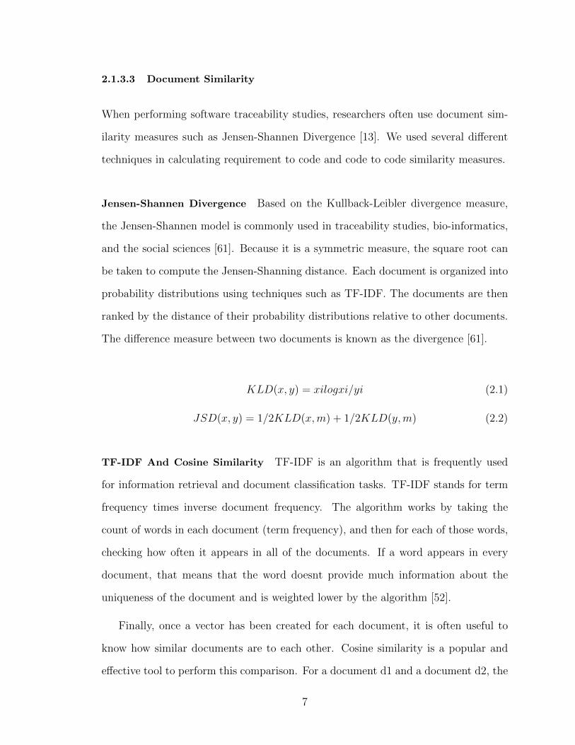
2.1.3.3 Document Similarity
When performing software traceability studies, researchers often use document sim-
ilarity measures such as Jensen-Shannen Divergence [13]. We used several different
techniques in calculating requirement to code and code to code similarity measures.
Jensen-Shannen Divergence Based on the Kullback-Leibler divergence measure,
the Jensen-Shannen model is commonly used in traceability studies, bio-informatics,
and the social sciences [61]. Because it is a symmetric measure, the square root can
be taken to compute the Jensen-Shanning distance. Each document is organized into
probability distributions using techniques such as TF-IDF. The documents are then
ranked by the distance of their probability distributions relative to other documents.
The difference measure between two documents is known as the divergence [61].
KLD(x, y) = xilogxi/yi (2.1)
JSD(x, y) = 1/2KLD(x,m) + 1/2KLD(y,m) (2.2)
TF-IDF And Cosine Similarity TF-IDF is an algorithm that is frequently used
for information retrieval and document classification tasks. TF-IDF stands for term
frequency times inverse document frequency. The algorithm works by taking the
count of words in each document (term frequency), and then for each of those words,
checking how often it appears in all of the documents. If a word appears in every
document, that means that the word doesnt provide much information about the
uniqueness of the document and is weighted lower by the algorithm [52].
Finally, once a vector has been created for each document, it is often useful to
know how similar documents are to each other. Cosine similarity is a popular and
effective tool to perform this comparison. For a document d1 and a document d2, the
7
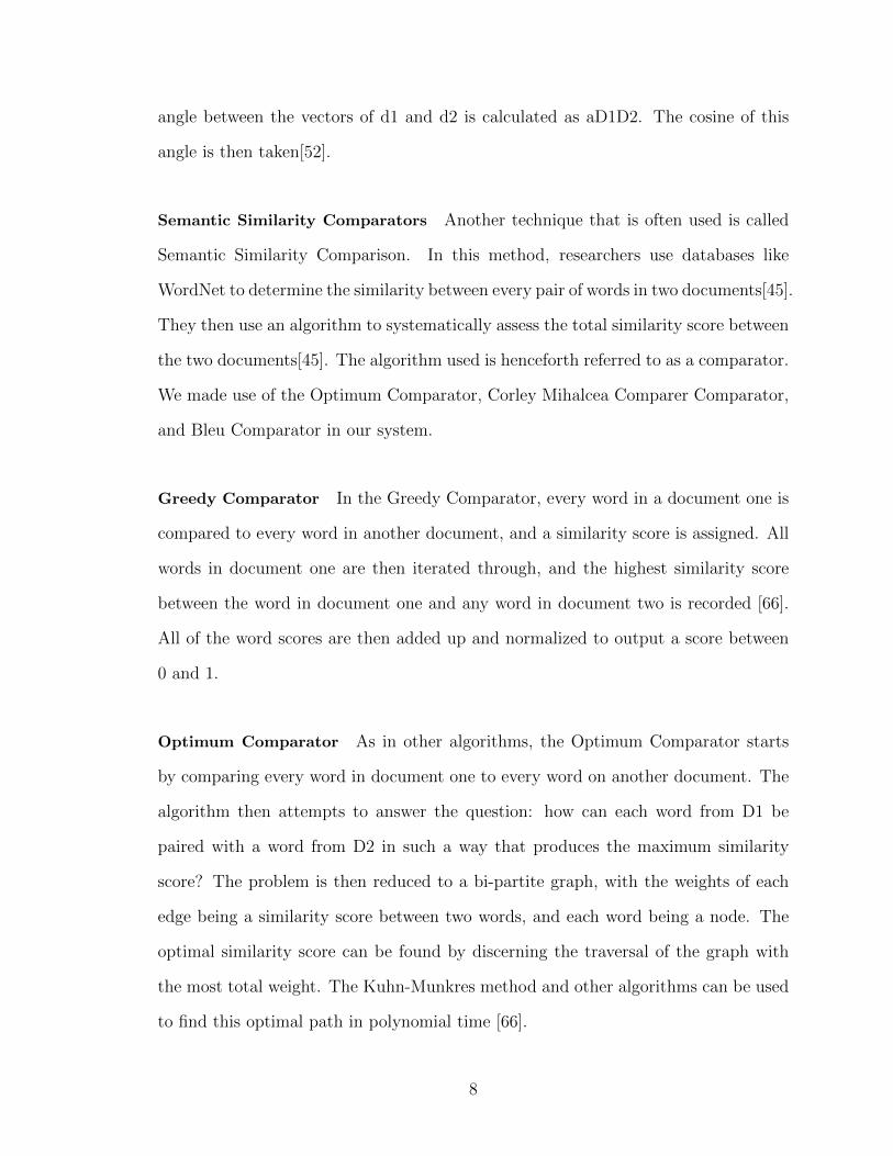
angle between the vectors of d1 and d2 is calculated as aD1D2. The cosine of this
angle is then taken[52].
Semantic Similarity Comparators Another technique that is often used is called
Semantic Similarity Comparison. In this method, researchers use databases like
WordNet to determine the similarity between every pair of words in two documents[45].
They then use an algorithm to systematically assess the total similarity score between
the two documents[45]. The algorithm used is henceforth referred to as a comparator.
We made use of the Optimum Comparator, Corley Mihalcea Comparer Comparator,
and Bleu Comparator in our system.
Greedy Comparator In the Greedy Comparator, every word in a document one is
compared to every word in another document, and a similarity score is assigned. All
words in document one are then iterated through, and the highest similarity score
between the word in document one and any word in document two is recorded [66].
All of the word scores are then added up and normalized to output a score between
0 and 1.
Optimum Comparator As in other algorithms, the Optimum Comparator starts
by comparing every word in document one to every word on another document. The
algorithm then attempts to answer the question: how can each word from D1 be
paired with a word from D2 in such a way that produces the maximum similarity
score? The problem is then reduced to a bi-partite graph, with the weights of each
edge being a similarity score between two words, and each word being a node. The
optimal similarity score can be found by discerning the traversal of the graph with
the most total weight. The Kuhn-Munkres method and other algorithms can be used
to find this optimal path in polynomial time [66].
8

Corley Mihalcea Comparator Introduced in 2005, the Corley Mihalcea Compara-
tor attempts to combine many word-to-word comparisons in order to produce a single
text-to-text comparison between two documents [58]. Like TF-IDF, it weights the
specificity of words using their inverse document frequency, so that an article like
”be” does not have the same weight as ”sheepdog”. Every word in document 1 is
compared with every word with document 2, with nouns and verbs being compared
via WordNet similarity, and all other parts of speech being compared lexicly. After-
wards, for each word in document one, the optimal similarity score in document 2 is
chosen. All of these scores are then added up and flattened into one score. This pro-
cess is then repeated for document 2 with respect to document 1, producing another
flat score [31]. The two scores are then averaged, producing a final Corley Mihalcea
score between 0 and 1.
Bleu Comparator The Bleu Comparator, invented to evaluate the aptitude of ma-
chine translations, works by evaluating the n-gram precision between two texts, pe-
nalizing the text for being overly or underly verbose [64]. A score representing the
quality of the translation from document D1 to document D2 is outputted on a scale
from 0 to 1. It is our hypothesis that a highly similar requirement pair will be ”trans-
latable” to one another, and thus have a high Bleu score[64].
2.2 Classification
In the realm of statistics and computer science, classification refers to the process of
predicting a label for a piece of data given a set of inputs [54]. The set of input data
is generally referred to as a set of features. Data Scientists attempt to manipulate a
dataset’s features to produce the most accurate classifications. More information on
9

the specific machine learning techniques used in CCP can be found in the Approach
and Evaluation chapters.
2.2.1 Supervised Machine Learning
A supervised machine learning classifier relies on a set of past inputs in order to make
future predictions [54]. This process is known as training. Oftentimes, researchers
will set aside a chunk of data to use for training, and another, usually smaller chunk
for testing.
2.3 Related Work
The following is a summary of previous research that is related to the CCP project.
Each study is highly related to either impact analysis or traceability.
2.3.1 Source Code Traceability
The study of source code traceability attempts to make connections between software
design materials and the resulting code [44]. Traceability mechanisms between soft-
ware architecture and code can ease the burden of software maintenance by making
the code easier to understand.
2.3.1.1 Event-based Traceability
Buchgeher and Weinreich introduced the LISA sytem to track and enforce traceabil-
ity. LISA required design engineers to use a semi-structured design language[44].
When software engineers made modifications to the software, they were required to
specify which active design decision they were working on. Next, software engineers
performed design implementation tasks, and these events were logged. The trace-
10

ability target was then evaluated. This differs from our task in that we do want to
analyze traceability independently of any proprietary design system or language.
Hammad et al. used a method that used various syntactic techniques to evaluate
whether a particular code change altered the software design [43]. They found that
changes such as adding or removing classes and methods often correlated with design
changes, while changes such as modifying data structures, conditional statements,
and loops did not. Their system works by first performing a diff of the code changes,
converting the diff to XML, and performing a variety of XPath queries to determine
what pieces of the code have changed. The tool then attempts to see what relation-
ships have changed. Our tool will differ from this one in that we want to predict
code changes based on requirements, while this tool simply analyzes the code that
has changed and categorizes it.
2.3.1.2 Traceability With Machine Learning Classifiers
There have been several studies that have utilized machine learning to find software
traceability links, many of them performed by researchers at DePaul University [29].
Cleland-Huang et al. performed an experiment to trace code back to its requirements
using an ML classifier. Using government regulatory codes, requirements, and the
traces, they were able to achieve of .807 for the Encrypt and Decrypt code, although
the algorithm was not this accurate across the board.
Mirakhorli et al. utilized two different classifiers for some of their research at
Depaul in 2012 [62]. First, they identified several different tactics or categories:
heartbeat, scheduling, resource-pooling, authentication, and audit-trail. They took a
code dataset and labeled each piece of code with a tactic for training, then built a
classifier which could predict the tactic for a piece of code. They also took several
descriptions of the tactics from text-books, labeled them, and built another classifier
11

trained on this data. They then created a classifier trained on different sub-roles for
each tactic, and it was run after all the classes were initially classified.
In 2014, Cleland-Huang et al. performed a study on the present and future of
software traceability. They detailed that most software traceability practices are
done manually, which requires extensive time and effort[30]. When traceability is
implemented, it is often done in a rushed manner at the end of a product life-cycle in
order to meet certification requirements. Cleland-Huang et al. note that it should be
the long-term goal of the software engineering community to construct an ubiquitous,
automated traceability tool. Many of the current traceability tools are imperfect;
they are either tailored for a certain project or lacking in accuracy. They posit that
a primary research goal should be to ”Develop intelligent tracing solutions which are
not constrained by the terms in source and target artifacts, but which understand
domain-specific concepts, and can reason intelligently about relationships between
artifacts” [30].
2.3.1.3 Relation To Our Project
Our project is related to traceability in that we are, in a sense, attempting to perform
some traceability analysis to link requirements back to java classes. Our classifier
differs from the DePaul studies in that we are seeking to build a classifier that does
not need to be trained on a pre-defined set of requirements; we want it to be trained
on a project’s specific set of requirements.
2.3.2 Impact Analysis
Impact analysis is the study of the work generated by a change request, with the
change request being something as formal as a requirements document, or something
more informal such as a bug-fix ticket. For example, oftentimes in industry today,
12

impact analysis is performed manually by software engineers on a case-by-case basis
[26]. The work generated by a change request is referred to as an impact set. An
impact set could consist of fine-graned elements as methods and single lines of code,
or course-grained elements such as a class file or package. When a change request is
made, the initial set of elements thought to need modification is called the starting
impact set. Once impact analysis is completed and work has been performed, the set
of elements that actually changed is called the actual impact set. This terminology
emphasizes the point that there are almost always unintended consequences to a
change request - the candidate impact set rarely matches the actual impact set.
2.3.3 Manual Impact Analysis
From 1996 to the mid 2000s, Shawn A. Bohner conducted a number of studies on
impact analysis. In 1996, Bohner performed a study detailing ways to integrate
impact analysis into the development process at the human level [22]. In 2003, Bohner
attempted a study of impact analysis in regards to changes to commercial off-the-
shelp components [21]. Keeping in mind the concepts of the starting impact set
(the changes estimated to be made) and the actual impact set (the actual changes),
Bohner detailed that software objects could be modeled as a dependency matrix or
graph, from which one could look at both indirect and direct impacts. Each Software
Lifecycle Object (SLO) could be thought of as being a certain distance away from
another SLO. SLOs that are a large distance from each other could be objects in
different modules, so making a change to one unlikely to affect the other. SLOs that
have a short distance are usually highly dependent on each other. With this measure
of distance in mind, Bohner then observed that using 3D visualization techniques was
useful in analyzing the actual impact sets.
13

In 1998, Mikael Lindvall and Kristian Sandahl performed a study on requirements-
driven impact analysis inspired by Bohner’s previous work [57]. They worked with
developers of the PMR project over two releases and four years, recording relevant
data for impact analysis. Based on the given requirements for a release, the devel-
opers predicted the C++ classes in the code-base that were likely to change. The
researchers measured the correctness of the predictions in terms of the successful class
predictions (true positives) against unsuccessful predictions (false positives), as well
as the completeness of the class predictions, which refers to the number of classes
expected to change vs. the number of classes that actually changed. For the first
release, the correctness of the predictions was 81%, and the completeness was 31%.
For the second release, the correctness was 86.1% and the completeness was 38.8%.
This shows that, in addition to requiring extra time and effort on the part of devel-
opers, manual impact analysis does not necessarily yield perfect results; even domain
experts of a software often produce candidate sets that are much different from the
actual impact sets for a given change.
2.3.4 Automated Impact Analysis
In 2005, Tsantalis et al. developed a tool to predict the probability of change for a
class using a system’s code base and its change history. Given a class’s dependen-
cies, summarized by its CKJM metric scores, and its history of change, their system
outputted a probability using logistical regression [69].
In 2011 study, Lehnert et al. categorizes the state of the art on impact analysis
research [56]. In addition to program slicing and information retrieval techniques,
researchers have used Call Graphs, where graphs are composed of function calls ex-
tracted from code, execution traces, where the software is analyzed for impact analysis
as it runs, Program Dependency Graphs, where dependencies between certain code
14

fragments are extracted, Probabilistic Models, using Markov Chains or a Bayesian
system to check how likely a change is to modify other code fragments, and History
Mining, where entities that often change together are analyzed.
More recently, in 2015, Acharya et al. performed a study on static program slicing
and its usefulness in impact analysis [15]. Static program slicing is the process of
isolating or slicing the code so that only a certain piece related to a certain function
is extracted. Acharya et.al created a tool called IMP which attempted to address
common issues with static program slicing tools, such as accuracy and performance.
This tool is heavily tied to the CodeSurfer API as well as Visual Studio, so is not
ideal for future open source development.
2.3.4.1 Predicting Class Changes Using Co-change History
In 2004, Ying et al. used association rule data-mining techniques along with past
class-change history to predict to predict future class changes [72]. Using a Fre-
quency Pattern Tree (FPTree) and a low min-support threshold, they developed an
association rule algorithm and ran it on the Eclipse and Mozilla projects. The devel-
oper would need to specify one file involved in the changes, and the association rules
would recommend the rest. Their tool was essentially a probabilistic recommendation
system.
More recently, in 2011 Eski et al. conducted an empirical study on object-oriented
metrics in order to predict change-prone classes [38]. They assigned different weights
to different code modifications, with something like a method change having a higher
weight than a field being added to a class. They computed the weights for each class
historically, and the classes with the top 10% most weighted scores were grouped
together as the most changed classes.
15

2.3.4.2 Predicting Software Changes From Requirements
There have been a few previous studies which have attempted to predict changes to
software based on either requirements, the previous code-base, or a combination of
both.
In 2005, Canfora et. al performed experiments attempting to identify the work
created, or files changed, as a result of the creation of Bugzilla tickets [26]. To do
this, they used information retrieval techniques. They looked at past change requests,
and if they were similar to the current change request, they took into account the
files those past requests modified. They used NLP techniques such as stemming the
words, computing word frequencies, and scoring the documents by relevance, using
an input requirement as a search query.
In 2013, Kim et al. worked on a system to predict what source code files would
change as a result of bug-fix requests [50]. They used the Mozilla FireFox and Core
code repositories as their corpus in tandem with the public Bugzilla database for
both. They built what was essentially a two-pass classifier. For the first pass, they
hand-tagged bug-fix requests as either ”USABLE” or ”NOT USABLE”, and then
trained a classifier based on natural language processing features to predict whether
the bug-fix request was usable. On most of the analyzed datasets, at least half of
the bug-fixes were filtered out in this manner. They did this because vague bug fix
requests will probably yield incorrect information to the end user. For the next pass,
they extracted all of the words out of each bug-fix request, stemmed all the words,
computed term frequencies, and filtered out all common stop-words. They then used
all of this information to create features for classification, along with the metadata of
the bug-fix request (system, epic, etc) and then trained the classifier. They claimed
70% accuracy on data that was actually usable [50].
16

2.3.5 Relation To Our Project
Our project is highly related to impact analysis, as on some level, we are trying to
predict the work created as a result of a requirement. Because manual impact analy-
sis is such a time-consuming and fault-prone endeavor, we are seeking to perform this
impact analysis in an automated fashion. Though our project does not fit neatly into
any of the categories named in Lehnert’s taxonomy, we do use elements of History
Mining (when extracting features related to how likely a class is to change), infor-
mation retrieval (when gathering various complexity and static metrics for a given
class), and probabilistic modeling (given that we train a machine learning classifier)
[56].
In particular, our research most closely relates to the studies of Canfora et al. and
Kim et al., in that we use past change request history and NLP similarity measures
to determine future software artifact changes. Our project also relates to Tsantalis
et al., in that we use class dependency and quality analysis to guide our prediction
of class changes.
17

Chapter 3
APPROACH
Our approach combines NLP, static analysis, CKJM metrics, and temporal locality
data into a single machine learning classifier. While there have been numerous studies
on traceability and bug prediction, we are not aware of another study that combines
both static analysis, object-oriented complexity, and NLP techniques to attempt to
predict class changes. We blend elements of both impact analysis and traceability to
produce a unique approach.
3.1 Linking Process
Unfortunately, most project management tools we tested are not directly linked to an
SCM. Thus, the CCP linker must perform some data-processing to determine which
data should be connected to which commits.
1. The linker attempts to link each requirement to one or more commits.
2. The linker calculates the approximate set of files present at the time of the
requirement, as well as the number of files touched as a result of the requirement.
3. Temporal locality is calculated (with care) for each requirement.
4. CCP then calculates the names and commit IDs of each release.
5. For each release, CCP performs static analysis.
6. For each requirement, its release ID is checked. CCP links release metrics to
requirements that are part of that release.
18

Figure 3.1: Relationship Between Requirements And Commits
7. Any externally computed metrics, such as VSM calculations, are linked in as
well.
The most central data structure in the linking process is that of a Require-
mentChange. A RequirementChange is simply a textual requirement that can be
directly linked to source code changes. Once the RequirementChange object con-
struction has been completed, it will contain several linked commits, a list of files
that were touched by those commits, and an approximate list of untouched files
present in the system at the time of the requirement’s creation. Each instance of a
class being touched or untouched will be used as a sample in the finished dataset.
3.1.1 From RequirementId To Commit
CCP relies on software developers following specific rules when performing commits:
they must specify the full ID of the originating requirement when performing a com-
19

mit. So, if a requirement is created named TIKA-11, the commit associated with
the requirement must have TIKA-11 in its commit message. Assuming the project
is named TIKA, the commit is evaluated with the regular expression .*TIKA-([0-
9]+).*.
When CCP parses all of the commits, it will check each commit for a valid re-
quirement ID. If a commit does not contain a valid requirement ID, it will not be
linked.
20
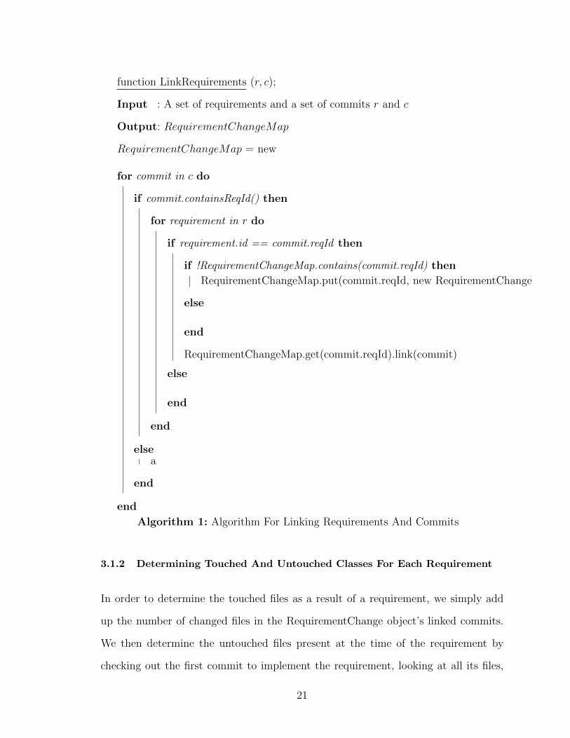
function LinkRequirements (r, c);
Input : A set of requirements and a set of commits r and c
Output: RequirementChangeMap
RequirementChangeMap = new
for commit in c do
if commit.containsReqId() then
for requirement in r do
if requirement.id == commit.reqId then
if !RequirementChangeMap.contains(commit.reqId) then
RequirementChangeMap.put(commit.reqId, new RequirementChange
else
end
RequirementChangeMap.get(commit.reqId).link(commit)
else
end
end
elsea
end
end
Algorithm 1: Algorithm For Linking Requirements And Commits
3.1.2 Determining Touched And Untouched Classes For Each Requirement
In order to determine the touched files as a result of a requirement, we simply add
up the number of changed files in the RequirementChange object’s linked commits.
We then determine the untouched files present at the time of the requirement by
checking out the first commit to implement the requirement, looking at all its files,
21

Figure 3.2: Requirement And Commit Life Cycle
then filtering out any files that were created after the requirement date. We filter out
any files that were present in our list of touched files.
This is not a perfect procedure, but we found it simpler and less error-prone than
other methods.
3.1.3 Determining Releases
Determining which commit is the first in a release can be difficult. Sometimes, users
do not tag software releases properly in the SCM repository. Or, they create many
extraneous ”tags” that are not actually releases. We thus employ a heuristic in order
to approximate the commit ID of a release. We assume that each requirement in the
project management software is marked with a release ID. We then, using our set of
linked requirements, look up the commit ID of the first requirement to implement
that release and record its parent commit ID. If we did not take the parent commit of
the first requirement in a release, we could risk effectively giving requirements data
from the future, invalidating our data.
22

Figure 3.3: Dataset Visual
3.2 Natural Language Processing
As the CCP system deals with textual requirement data, we employed sophisticated
NLP techniques in order to synthesize this data. Below is a summary of methods
used in our textual pre-processing and similarity calculation steps.
3.2.1 Pre-processing
Our pre-processing methodology is fairly similar to standard methods[46]. First, we
remove any characters not related to the English language, such as ’@’. We do this
because such characters are often extraneous and don’t contain much meaning; they
could indicate a requirement as more unique than it actually is.
We then split up ’CamelCase’ class, method, and variable names, so ”GitExtractor
becomes” git extractor, and ”bankPostRoutine” becomes ”bank post routine” files.
23

This is because a requirement will often contain text such as ”Please modify the bank
post routine to do x”. If we simply left ”bankPostRoutine” in-tact, the requirement
text and the code text wouldn’t have the words ”bank post routine” in common, and
thus we’d miss valuable similarity information.
Finally, we stem each word using the Porter stemmer. The Porter Stemmer works
by running a word through a series of rules until the word has been truncated in such a
way that no more rules can be applied [46]. For example, consider the word ”agreed”.
The stemmer might have a rule saying that if a word has a vowel, a consonant, and an
”eed” ending, remove the ”d”, which leaves us with ”agree”. Stemming allows us to
reduce different grammatical forms of a word to the word’s stem [46]. This allows us
to filter words like ”agreement” and ”agreeing” down to their base stem of ”agree”.
This helps us to accurately match words based on their intended meaning, improving
accuracy scores.
3.2.2 Requirement Similarity
One of our new research contributions is the ability to historically compare require-
ments that have modified a class. Every time a class is touched, we make note of
the past requirements that the code change implemented. We hypothesized that past
requirements that changed a class should be similar to current requirements that
modified a class. They will probably at least have certain key-words in common.
Below is an example of two requirements which both led to implementation of the
same class.
R1:
“We should define what happens in a SortedKeyValueIterator whenhasTop, next, getTopKey, and getTopValue are called before init andbefore seek. We should expect the defined behaviors in tests, and wherepossible we should enforce those behaviors.”
24

R2:
“The iterator options for input formats are packed into a single stringand delimited with colons and commas. The options aren’t escaped, sothey cannot contain the delimiter characters. This should be documentedand/or fixed.”
Keeping a list of the past ten requirements that changed a class (prior to the
current requirement), we calculate the semantic similarity comparators of each re-
quirement. We then compute the maximum, median, and average of the top five
scores for each requirement.
25

Figure 3.4: Requirement To Requirement Similarity Example
26

Compute requirement to requirement similarities
for all requirement do
for all class in requirement do
last10 = compute last 10 requirements that touched the class
similarities = computeSimilarities(last10)
for all similarityList in similarities do
featureList = new list
featureList.add(average(similarityList, requirement))
featureList.add(averageTopFive(similarityList, requirement))
featureList.add(max(similarityList, requirement))
output(featureList)
end for
end for
end for
computeSimilarities Compute the Similarities using each algorithm
algorithmList = [BlueComparator, CorleyMihalcea, GreedyComparator,
OptimumComparator, jensenShannon, VSM]
similarities = new list
for all algorithm in algorithmList do
for all requirement in last10 do
similarities.add(algorithm(requirement, originalRequirement))
end for
end for
return similaritiesAlgorithm 2: Algorithm For Computing Requirement To Requirement Similarities
27

3.3 Temporal Locality Calculation
We computed several different features based a class’s history of being modified. Our
reasoning was that if a class had been modified in the past, it would be more likely to
be modified in the future. As you can see from these project results, we found that
past modifications do have a correlation with future modifications.
We then wanted to include some concept of temporal locality - which is the concept
of more recent modifications being more important than older modifications. Kim
et al. pioneered the use of temporal locality in predicting software changes, building
a variety of caches to weight the importance of prior software modifications [51].
Bernstein et al. rolled up the number of modifications for a class by month for the
most 6 recent months, and used those temporal features to train a defect-predicting
classifier[20]. With both of these concepts of temporal locality in mind, we developed
two new metrics to measure the temporal locality of recent modifications for each
class.
For the below formulas, k is the number of modifications for the class as well as the
index of the oldest modification. The letter n denotes the total number of commits
involving the class, whether it was touched or untouched. The letter i represents
number of the current modification, with the most recent commit involving the class
having index 1. The closer the modification is to index 1, the most recent modification,
the more weight it will be given.
3.3.1 Simple Modification %
For the simplest of our history score calculations, we divided the number of times
the class had been touched up until that point in the history by the total number of
commits where that class existed. Though this computation was rather simple, we
28

found it to be a useful feature.
k
n(3.1)
3.3.2 Linear Temporal Locality Modification Score
For the next of our temporal locality calculations, we incorporated temporal locality.
We store a map of each class and its history of modifications, calculating a score that
lends more weight to recent class modifications. Given that the most recent commit
index is 1, the modification of the class at commit index 2 will be given a weight of
.5, the modification at index 3 will be given the weight 1/3, etc. All of these weights
will then be divided by the total number of commits where the class had existed up
until that point in time.
∑ki=1
1i
n(3.2)
3.3.3 Logarithmic Temporal Locality Modification Score
We found that on occasion, the previous method gave older modifications too little
weight. We found that by instead of dividing by k, dividing by ln(k) when k is greater
or equal to 3 gives us a sufficient amount of temporal locality. The weight decays
much more gradually than with the previous method. So, the modification at commit
index 4 will be given a weight of 1 / ln(4), the modification at commit index 5 will be
given a weight of 1 / ln(5), etc. Again, all weights will then be divided by the total
number of commits where the class had existed up until that point in time.
∑ki=3
1ln(i)
n(3.3)
29

3.3.4 Example Calculations
To better understand the calculation of temporal locality scores, it is useful to map
out a simple example. Given the table below, six different requirements have been
processed, and there are three different classes in the dataset.
For the simple calculation, we see that class A has been touched 4 different times,
so the modification percentage would be four divided by six or two thirds. Class
B has been touched three times, and there are a total of six requirements, so the
modification score would be one half. For the linear calculation, we start taking into
account the temporal localities of the class modifications. Class A has been touched
at its sixth oldest modification, so we add one sixth to our running total. Class A
was also modified at its fifth-most, fourth-most, and third-most recent commits, so
we add that all to the running total, divide by 6, and end up with a score of .16.
Class B has more recent modifications, but less total modifications, but we can see
that it still has a higher score at .18 than class A does. Class C has the least total
modifications with only 2, but it has the highest linear temporal locality score at
.25. This exemplifies how heavily the linear temporal locality method favors newer
modifications. The logarithmic calculation works very similarly to the linear calcula-
tion, but we can see that it penalizes older activity substantially less than the linear
method. For class A, we take one divided by ln of 6 plus one divided by the ln of 5
plus one divided by the ln of 4 plus one divided by the ln of 3, then divide this all by
6, producing a score of .47. Running the numbers in a similar fashion for B, we are
left with a score of 0.44, and 0.33 for class C.
To reinforce these concepts, let us go through a more advanced example. Suppose
we have a class, Connector.java, that we want to produce temporal locality scores for
as time passes by. When we are given the first ever requirement, no files as of yet
30

Table 3.1: Example Of Temporal Locality Result For Three Classes
Class Requirement Touch Temporal Locality Results
Name 1 2 3 4 5 6 Simple Linear Logarithmic
A X X X X 0 0 0.67 0.16 0.47
B 0 0 X X X 0 0.5 0.18 0.44
C 0 0 0 0 X X 0.33 0.25 0.33
have been modified, so the temporal locality scores are all 0. Suppose then that the
class is touched in the first requirement. For the second requirement, we have had a
total of one requirement, and that requirement modified the Connector.java class, so
each temporal locality score is 1. Requirement 2 does not modify the class. So now at
requirement 3, the class has been modified 1/2 times for a simple score of .5. For the
weighted score, we calculate 1/2 / 2 to arrive at a score of .5. Since our logarithmic
algorithm does not start taking logarithms until requirement 3 or greater, the score
is also .5 here.
At requirement 4, we have a history of 3 total requirements, with modifications at
requirement 1 and requirement 3. The simple score is 2/3, the weighted score is (1/3
+ 1) / 3, and the logarithmic score is (1/ln(3) + 1) / 3. Here, we can already see the
contrast between the different algorithms. The older a change is, the less the weighted
algorithm places on the importance of the change. The logarithmic algorithm has the
same philosophy, but does not penalize older changes quite as much.
At requirement 5, we have a history of 4 total requirements, with modifications
at 1, 3, and 4. The simple score is 3/4, the weighted score is (1/4 + 1/2 + 1) / 4.
The logarithmic score is (1/ln(4) + 1 + 1) / 4.
Now let’s skip ahead to requirement 8. We have a history of 7 total requirements,
with modifications of Connector.java at 1, 3, and 4. The simple score is 3/7, the
31

weighted score is (1/7 + 1/5 + 1/4) / 7 for a total of .084, and the logarithmic score
is (1/ln(7) + 1/ln(5) + 1/ln(4)) / 7 for a total of .265. Note how much the weighted
and logarithmic temporal locality scores drop without any recent modifications.
At requirement 9, we finally have another recent modification. There is a history
of 8 total requirements now, with modifications at 1, 3, 4, and 8. The simple score
is .5, the weighted score is (1/8 + 1/6 + 1/5 + 1) / 8 for a total of .186, and the
logarithmic score is (1/ln(8) + 1/ln(6) + 1/ln(5) + 1) / 8 for a total score of .332.
It is interesting to see how much the logarithmic and weighted scores jump up once
there are more recent modifications.
At requirement 14, we have a history of 13 total requirements, with modifications
at 1, 3, 4, 8, and 9. The simple score has droped to 5 / 13 for a total score of .3846,
the weighted score is (1/13 + 1/11 + 1/10 + 1/6 + 1/5) / 13 for a total score of .048,
and the logarithmic score is (1/ln(13) + 1/ln(11) + 1/ln(10) + 1/ln(6) + 1/ln(5))
/ 13 for a total of .186. Again, note how sharply the temporal locality scores drop
when there are no recent modifications.
3.4 ML Classifier
Once all metrics have been calculated and serialized, we create one sample per instance
of a touched or untouched class file associated with a RequirementChange. We add
in the NLP, static analysis, and temporal locality metrics for each sample, then use
this data to train a classifier that makes a simple binary classification - touched or
untouched.
32

Table 3.2: Temporal Locality Example
Class ReqId Previous Modifications Simple Weighted logarithmic
Connector.java 1 None 0 0 0
Connector.java 2 1 1 1 1
Connector.java 3 1 .5 .25 .5
Connector.java 4 1,3 .67 .433 .6366
Connector.java 5 1,3,4 .75 .4375 .68
Connector.java 8 1,3,4 .429 .084 .265
Connector.java 9 1,3,4,8 .5 .186 .332
Connector.java 14 1,3,4,8,9 .3846 .048 .186
3.4.1 Feature Pre-processing Configurations
We employed two different feature pre-processing configurations when training and
testing our classifier. They are as follows.
3.4.1.1 Principal Component Analysis
Many models contain features that are either extraneous or highly correlated with
other features. Principal Component Analysis, or PCA, is often used to reduce dimen-
sionality in datasets [47]. First Introduced by Pearson, PCA bears many similarities
to the process of Singular Value Decomposition in linear algebra. If we consider a
matrix, M, which is an NxP matrix with N values and P variables (or features), we
can construct a diagonal variable matrix by taking V=MM/(n1) [47]. The eigenvec-
tors for this data are called the principal directions, and projections onto this space
are called the principal components [47].
33
Once PCA is performed, we are left with an approximation of the original matrix
that still contains valuable information, but with less variables used. The variables
used will often effectively be combinations of variables from the previous matrix M,
and should all be independent from one another [70].
We utilized PCA as one of our two feature pre-processing configurations.
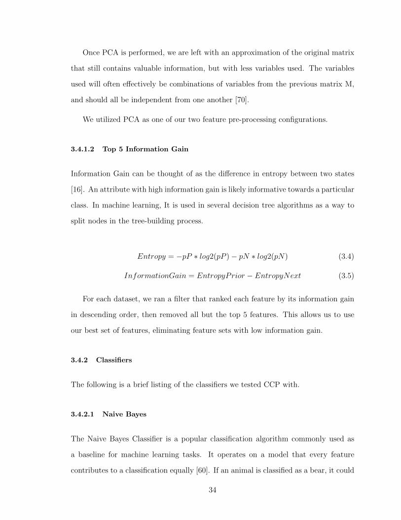
3.4.1.2 Top 5 Information Gain
Information Gain can be thought of as the difference in entropy between two states
[16]. An attribute with high information gain is likely informative towards a particular
class. In machine learning, It is used in several decision tree algorithms as a way to
split nodes in the tree-building process.
Entropy = −pP ∗ log2(pP ) − pN ∗ log2(pN) (3.4)
InformationGain = EntropyPrior − EntropyNext (3.5)
For each dataset, we ran a filter that ranked each feature by its information gain
in descending order, then removed all but the top 5 features. This allows us to use
our best set of features, eliminating feature sets with low information gain.
3.4.2 Classifiers
The following is a brief listing of the classifiers we tested CCP with.
3.4.2.1 Naive Bayes
The Naive Bayes Classifier is a popular classification algorithm commonly used as
a baseline for machine learning tasks. It operates on a model that every feature
contributes to a classification equally [60]. If an animal is classified as a bear, it could
34

have features such as size = large and fur = brown, and each of these features would
independently contribute to the classification. After training, each feature is given a
probability for a classification called the posterior probability. It then takes the prior
probability of the given class if there were 30 bears classified out of 60 animals in
the training set, this would be a probability of 0.5. This is then multiplied by the
combined probability of the features for the given class, which forms what is known
as the posterior probability (evidence is a constant, and can be ignored for the sake
of this explanation) [60]. The class with the highest posterior probability is chosen.
3.4.2.2 Bootstrap Aggregation
Bootstrap aggregation, otherwise known as bagging, is an ensemble classifier, which
means that it is an external algorithm that creates additional classifiers based on
different parts of the data.
Bootstrap Aggregation consists of two actions: bootstrapping and aggregation.
In the bootstrapping portion, the data is sampled repeatedly with replacement. A
classifier is then trained on each group of samples. When testing, several classifiers
attempt to predict a sample, with the mode classification chosen [23]. The algorithms
for bootstrapping and bagging are defined as follows.
• Assume we are splitting the data into k chunks
• Sample a random chunk of the data
• Sample the rest of the data into k - 1 additional chunks, with replacement
35

Building multiple classifiers
for all Chunks from i to N do
Create a training set from chunk i
Train a classifier on chunk i
end for
Testing
for all samples j to A do
Test each classifier on the sample.
The mode classification is chosen.
end forAlgorithm 3: Bagging
3.4.2.3 Decision Tree
A decision tree is is a graph representing various pathways that can be taken, given a
set of variables, with a nominal result, or class label, at its leaf nodes [16]. Decision
Trees are usually built from the top down, using a breadth-first or depth-first search,
placing nodes with the highest information gain towards the top of the tree [16].
To increase the accuracy of the decision tree, most algorithms employ some form of
pruning of the tree, effectively removing branches of the tree that are less useful in
performing classifications [16].
3.4.2.4 The J48 Decision Tree
The J48 Decision Tree is an implementation of the C4.5 Decision Tree algorithm
using the java programming language. The C4.5 algorithm, like other decision tree
algorithms, starts by building a tree from the top down. As the tree is constructed,
the tree is split on nodes that yield the highest information gain, which can be thought
of as the difference in entropy between the two nodes [71]. Once the tree is finished,
36

the top-most nodes from the root should all have one or more branches leading to
unique classifications [71]. The algorithm then prunes the tree, putting leaves in place
of branches with low usefulness.
3.4.2.5 Random Forest
The Random Forest classifier is an evolution of the decision tree, where a number of
separate, randomized decision trees are generated. It is quite similar to the previously
introduced bagging algorithm as well, but differs in that when creating decision trees,
there is some randomness when choosing what feature to split on. In similar fashion
to bagging, once all the trees have been generated, the label with the most consensus
among the trees is chosen. This technique has proven to be highly accurate and
robust against noise [24]. However, because this classifier requires the building of
many different decision trees, it can be extremely expensive to run on large datasets.
3.4.3 Cross-Validation
Cross-validation refers to the process of splitting a dataset into N randomly separated
chunks. The chunks are then iterated through; at each iteration, one chunk is held
out for testing, while the classifier is trained on the remaining N - 1 chunks. The final
accuracy metrics are the result of testing all N chunks. Researchers often prefer n-
fold cross-validation to simple training/test splits, as N-fold validation employs more
rigorous evaluation of the dataset, ensuring that a model less likely to be overfitted
[17].
37

Chapter 4
CLASS CHANGE PREDICTOR
CCP is a complex system consisting of many moving parts. In this chapter, we discuss
the various technologies and tools that operate the machinery of CCP. The user must
first locate a relevant Git repository and a jira URL for the project. CCP can then
be configured to access its data stores and metric providers. Through commandline
invocations, CCP then gathers data using the configured values. Finally, CCP outputs
a variety of different data files, each of which is used to train a machine learning
classifier.
4.1 Data Stores
The Class Change Predictor draws from two main data sources in order to perform its
predictions on a given software project: the project’s code-base, which is historically
tracked in a version control system, and the project’s issue tracking software, which is
tracked via a web-based tool. This combination of textual and technical data allows
our system to gain a sophisticated understanding of what situations lead to software
changes.
4.1.1 Jira
Jira is a software management and issue tracking system commonly used in industry
[10]. It is used by commercial tech giants such as Amazon, as well as on open-
source Apache projects [10]. Software Development Managers (SDMs) can use Jira
to create teams, create projects, and break those projects up into subtasks. Software
38

Figure 4.1: System Workflow
39

Development Engineers (SDEs) can then take on certain subtasks or create new tasks
associated with a specific release.
We chose to focus on Jira systems for our data collection both due to the large
amount of openly browsable jira repositories available, as well as the ease of pulling
data out of jira with simple JQL queries.
4.1.1.1 Jira Extractor
Large projects usually have thousands of Jira issues, while most open Jira systems
usually place a limit on the amount of Jira issues that can be downloaded at a time
(typically 100) [10]. Thus, we devised a way to break up our request into several
different jira queries, pulling a small number of issues at a time, scraping the HTML
into a usable Jira Issue object, and parsing the results into a csv file.
Our Jira data scraping tool finds the first commit date in the repository, and then
performs many time delimited jira queries until all issues in the system are collected.
The scraper has proven to be robust across many different projects.
1. The scraper takes the first requirement date for a project.
2. The scraper downloads the tickets one hundred at a time, split up by week (no
week in any of the repositories had more than 100 tickets in a seven day period).
3. Scraped the HTML list of tickets into a simple CSV format and outputted a
final jira CSV file.
4.1.1.2 Parsing Jira Data Into Requirements
Each Jira change request is parsed into a Requirement object. A requirement contains
several key fields from the Jira Request, such as
40

• The Jira ID of the requirement.
• The summary text of the change request.
• The type of request, such as ”Bug”, ”New Feature”, ”Improvement”, or ”Task”.
• The release that the requirement is apart of.
• The creation date of the requirement.
Later on in the process, additional fields are added to link a requirement with the
state of the code repository at the time.
4.1.2 Git
Git is a version control system that is widely used in the software development com-
munity [8]. Git users can make changes to a software project, revert changes, make
branches for divergent code, and check out specific commits which correspond to the
version of a software at a specific point in time. It differentiates itself from SCM tools
like SVN in that git allows users to download a copy of the entire repository locally
[8].
We chose projects with Git version-control systems due to Git’s ubiquity, ease-of-
use, and API support. On a release by release basis, we leverage Git to find and store
the state of the code-base. This includes all source code files currently currently in
the repository and their associated metadata. This information is stored, to be used
at a later time for static analysis and NLP. On a commit by commit basis, we use
Git to find what files changed and what files stayed the same.
41

4.1.3 JGit
We used the JGit API due to its excellent documentation in comparison to other
libraries [9]. It is designed to be light-weight, and implements virtually all of Git’s
core functionality.
4.1.3.1 Git Extractor
Leveraging the JGit API, we created a custom Git Extractor tool. The Git Extractor
tool can iterate through all commits, record metadata about the commit, find out
what files have changed in the commit, and find out what files have stayed the same
in a commit. To facilitate this, we developed several custom methods.
• getAllFiles, which, given a commit as input, returns a list of tuples containing
all files currently in the repository, and their creation times.
• getFirstCommitTime, which returns the commit time of the first commit in the
repository.
• getChangedFiles, return all files that have changed as a result of the current
commit.
• filterFiles, which returns all files in the repository that have been created after
a certain time.
4.2 Build Tools
Building enterprise-scale projects can often prove a challenging task. Large-scale
projects typically depend on many external libraries, require specific build commands
and flags, and sometimes use disparate versions of programming languages. As such,
42

we developed our system to be robust, with the user able to input custom build
commands into the configuration file. CCP has been tested thoroughly using Apache’s
Maven, but it would also be easy to support other utilities, such as Make, using CCP’s
XML configuration file.
4.2.1 Maven
Maven is a dependency analysis and software package management tool for the java
programming language[3]. Developing robust java programs often requires down-
loading many external java packages that might depend on very specific versions of
each other. Developers use Maven to ease the pain involved in this process; develop-
ers can specify a central package, and then Maven constructs a dependency graph,
downloading and building all additional necessary packages.
For Java projects, we preferred to build with the Apache Maven tool, as Maven can
analyze a project’s dependencies, download all of the needed libraries from maven’s
central database, and then build the project [3]. As Maven is itself an Apache project,
almost all of the Apache software projects we surveyed were built using Maven.
Both SonarQube and CKJM require compiled bytecode to generate complete met-
rics for Java classes, so Maven’s ability to ease the build process of complex projects
is critical.
4.3 Release Metrics Storage And Tools
CCP gathers CKJM and SonarQube metrics static analysis metrics at the point
of each software release. This release data is stored in a data structure consisting
of a series of nested hashmaps, indexed by release, class name, and metric name
43

Figure 4.2: A Maven Dependency Graph
44

Figure 4.3: How The System Snapshots Releases
respectively. We have constructed several tools to facilitate interacting with these
two systems and extracting metric data.
4.3.1 SonarQube
SonarQube is a software analysis tool that can track metrics such as technical debt,
code smells, and lines of code [67]. It is commonly used by software development
teams to track the evolution of code quality over time [67]. It is configured with
Map o f Re lease S t r ing to
Map o f Class S t r ing to
Map o f Metric S t r ing to
Numeric metr ic Value
Figure 4.4: Map Of Metric Storage Structure
45

a variety of quality rules out-of-the-box, and developers can create unique rules at
will. Though we primarily used SonarQube to extract static analysis metrics, CCP
could be configured to gather dozens of other metrics from SonarQube on a per class
basis. For this reason, we chose SonarQube over simpler static analysis tools that
just compute the number of code smells, such as FindBugs.
4.3.1.1 SonarQube Executor
Once all releases (and their corresponding names and commit ids) have been extracted
from the project, the SonarQube executor is executed for every release. To ensure
the quality and correctness of the SonarQube data, we delete all existing data for a
project from the SonarQube database before checking out a release. Once a release is
checked out, the SonarQube Executor executes the Sonar Runner service to analyze
the current state of the given software project. This often takes several minutes,
depending on the size of the project. There is also usually some delay between
when SonarRunner finishes and when the project data is actually available for API
calls. Because of this, we developed the SonarQube executor to perform periodic
HTTP requests to confirm the project’s readiness for API calls. Once the SonarQube
Executor receives a successful confirmation, it signals to the SonarQube Scraper that
data is ready for analysis.
4.3.1.2 SonarQube Scraper
We built a robust tool to facilitate the extraction of SonarQube metrics from large
software projects. Our tool pulls data from SonarQube via HTTP Get commands
with the JSON option specified to be true. We parse the JSON metric data into
HashMaps, using the name of the class as a key to another HashMap with filenames
46

as keys and floating point numbers as values. All of the computed metric data is then
serialized to a file for later use.
4.3.2 CKJM Extractor
We first modified the open-source CKJM project to expose the ClassMetrics class,
as well as methods to gather all CKJM data without resorting to command-line calls
[68]. We then removed the command-line interface to the project, and added our own
method to parse all CKJM metrics for all compiled classes in a project. We compiled
all of this into a JAR file and included it in our CCP project. Given a directory, our
modified CKJM JAR will look for all .class files and compute the metrics for each
separate class, and then look for any .jar files and compute the CKJM metrics for all
the classes therein. Because CKJM requires java bytecode files, CCP only gathers
CKJM metrics for java development projects.
When a release has been checked out and the target project has finished building,
the CKJM extractor runs, extracting CKJM data for each class file, and storing this
data inside of the Release Metrics hash map.
4.4 Other Technologies
4.4.1 The Semantic Similarity Toolkit
We made use of the Semantic Similarity Software toolkit, otherwise known as Semilar,
in order to produce similarity scores between text. We chose this tool because of
maturity of its API - it provides a variety of different ways to determine similarity
between sets of text. More information on the various similarity calculations used
can be found in the approach section.
47

4.4.2 Weka
The Weka library is a machine learning toolkit developed by the University of Waikato
[12]. We made use of the Weka machine learning library due to its ease of use, wide
array of classifiers, and robust pre-processing tools[12]. Weka contains a total of 83
classifiers and at least 50 processing utilities. Using our system, users can train a
JF48 classifier and test its accuracy via a command-line call.
4.4.2.1 Attribute-Relation File Format
The Attribute-Relation File Format, or ARFF, was designed for use with Weka by
the the University of Waikato. ARFF files consist of header and data sections. The
header section, denoted with @Header, contains the names of each attribute used
in the file. The data section, denoted with @Data, contains all rows of data, called
instances. By convention, the class label is typically placed as the last of the data’s
attributes. It is a convenient, human-readable format in which to store training data.
Once CCP has completed processing necessary requirement, commit, and static
analysis data, it processes this information into several ARFF files. One file is created
for each feature, each feature group, and all of the combined features. In addition,
CCP performs PCA and generates additional PCA files for each feature group, as
well as for all of the combined features.
4.5 Configuration And Operation
In order to support a variety of different types of projects, we made the CCP tool
extremely customizable by utilizing an XML configuration file, as well as providing
the ability to use command-line arguments.
48

Table 4.1: Configuration Options
Option Purpose
git repo The location of the Git repository to be analyzed.
jira file The file name of Jira file to store requirements data in.
jira url The URL of the jira repository that will be queried.
req limit (Optional) The number of requirements to process before exiting
the linking phase. Useful for testing.
jira url The URL of the jira repository that will be queried.
statics file The location on disk of the serialized file that holds
static metrics.
sonar command Command used to run SonarQube on a project.
sonar host URL of the SonarQube server to extract data from.
sonar project Project name to use for the sonar repository. Defaults
to the name of the git repo.
sonar metrics Comma-separated list of metrics to extract for each class
from SonarQube.
4.5.1 Configuration
A variety of configuration options are available, the majority of which are required
for operation of the tool. A table listing the available configuration options, as well
as an example XML configuration file, are provided.
4.5.2 Commandline Operation
A variety of commandline flags and options are provided to ease the operational
burden for users of CCP.
49

Table 4.2: Command-line Flags
Flag Use
config Used to specify the XML configuration file to load settings from.
Mandatory
jira Run the Jira Scraping utility, then serialize the results to disk.
reqnum Similar to the XML option, specify the number of requirements to
process.
reqs Process all requirements, link them to commits, and serialize the
requirements to disk.
statics Run static analysis on every release, serializing the results to disk.
bigtable Generate a single table file with all combined metrics.
split Used to re-organize a training and test so that ”perfect” require-
ments appear at the beginning of a file
arff Used to indicate the need to dump all data to weka-formatted
ARFFs, split up by feature groups.
exclude missing When processing data, filter out lines with missing metric values
delete untouched Remove requirements from the dataset that aren’t associated with
any touched java or php files.
join When the user specifies a comma seperated list of serialized metrics,
this flag is used to join all the metrics into one file.
language Used to specify the programming language used in the project.
Defaults to Java.
report releases Output a report with release statistics.
report requirements Output a report with requirement statistics.
50

4.6 Overall Process
The typical workflow of the CCP system is listed below. This is by no means com-
prehensive, as it omits the use of several non-essential pre-processing capabilities
1. The user must first clone the target project Git Repository (manual).
2. The user then prepares project configuration file (manual).
3. The user then runs CCP.
4. CCP Iterates through the list of requirements. Each ticket is associated with
one or more commits from the repository. A list of formatted requirements is
serialized into multiple files.
5. CCP prepares a list of releases for the project. To figure out the commit hash
for each release, we take the first ticket to implement the release, then take
its parent. We are technically using the parent of each release, but this makes
some sense. We want the state of the code just before the release in order to
accurately predict what the release will implement.
6. For each release, CCP checks out the commit for that release, builds the project,
runs sonarqube for that project, runs ckjm, and extracts all the metrics.
7. After an outside source computes requirement to requirement and code to re-
quirement semantic similarity metrics, CCP incorporates these metrics into each
line of the final file.
8. CCP parses the combined data for each class into ARFF files required by Weka.
Two ARFF files are produced for each metric group: one with PCA performed,
51

and one without PCA performed. Split each individual metric into its own file.
Finally, CCP outputs two files for all of the combined metrics: one with PCA
performed, and one without PCA performed.
9. CCP then analyzes, trains, and tests the ARFF files using Weka with tenfold
cross-validation. This step can also be performed by a human manually using
the weka explorer interface.
4.6.1 Operation Scenarios
Due to the wide variety of command-line and configuration options, the operation of
CCP may seem daunting. To aid in the use and understanding of CCP, some common
operation scenarios are provided below.
4.6.1.1 Scenario 1: Compute And Serialize Requirements
In our first scenario, a user has configured an xml file called ”tika.xml” and filled in
all appropriate fields. She wishes to run the jira scraper tool, parse those jira issues
into requirements, link all the requirements to commits, and output a text file with
a list of all serialized requirements. She executes the following command.
−c o n f i g t i k a . xml j i r a r eqs
CCP then executes the jira scraper tool and the requirement parsing tool, outputting
several files, among them:
• A file listing each class found in the target software project.
• A file listing all of the requirement text found in the software project
• A file listing all releases in the project, and its associated commit ID.
52

• A file listing all requirements in the software project, which links to previous
files.
• A file listing all issues tagged as Bug fixes in the software project.
4.6.1.2 Scenario 2: Analyze Releases
The user wishes to perform static analysis on each release. The user wishes to link
the requirement change data and the associated metrics for each file all together in
one output table. She runs the following command.
−c o n f i g t i k a . xml s t a t i c s b i g t a b l e
In sequence, CCP runs static analysis for each release, then runs the ”big table”
routine, which links all available metrics together inside one file.
4.6.1.3 Scenario 3: Prepare ARFF Files
The user wishes to generate ARFF files to be used to train Weka machine learning
classifiers. She runs the following command.
−c o n f i g t i k a . xml a r f f
CCP analyzes the ”big table” file generated earlier, then generates ARFF files for this
table, as well as for each group of metrics in the table, and each individual metric in
the table. A total of 44 different ARFF files are generated.
4.6.1.4 Scenario 4: Ensemble
The user wishes to run all the previous steps again, in order. She executes the
following command.
−c o n f i g t i k a . xml j i r a r eqs s t a t i c s b i g t a b l e a r f f
53

CCP runs all of the previous steps, in order. CCP outputs several requirements-
related files, a file representing the serialized static analysis files, and at least 44
different ARFF files.
54
Chapter 5
EVALUATION
To evaluate the system, we used CCP to gather datasets from four different projects
of varying sizes. We performed one-hundred times ten-fold validation using seven
different classifiers and two different feature configurations.
5.1 Variables
For our experiments on the three java projects, we utilized 34 different independent
variables as well as three different dependent variables. A brief summary of these
variables follows.
5.1.1 Dependent
For our dependent variables, we ran our experiments and the results using the de-
pendent variables precision, recall, and 0.5F-Measure. The reasoning behind each
dependent variable is as follows.
5.1.1.1 Precision
In terms of our system, we measure true positives (TP), false positives (FP), true
negatives (TN), and false negatives (FN) as follows.
• TP: A class file is successfully predicted to have changed.
• FP: A class file is unsuccessfully predicted to have changed.
• TN: A class is successfully predicted to remain unchanged.
55

• FN: A class is predicted to remain untouched when it actually changed.
Precision is a measure of true positives divided by the number of false positives
added with true positives. For the CCP system, it is imperative that the system
maximizes true positives while minimizing false positives. A true positive indicates
that a class has changed. Incorrectly classifying a class that needs to be changed
could lead to wasted effort by a developer, including but not limited to a developer
refactoring a class that does not need to be touched. We thus weight the importance
of precision as a dependent variable higher than recall, as precision penalizes false
positives, while recall penalizes false negatives.
Precision =TP
FP + TP(5.1)
5.1.1.2 Recall
Recall measures the number of true positives divided by the number of true positives
added with the numbers of false negatives. Recall has a major weakness in that a
classifier choosing every entry of positive will have a recall of one; recall does not
penalize false positives.
Recall =TP
TP + FN(5.2)
5.1.1.3 F 0.1 Score
Even though precision is objectively the most important measure for the CCP sys-
tem, F scores also provide valuable evaluation data. The F0.1 score combines both
precision and recall in to one averaged score. While the traditional F1 score takes
the harmonic mean between precision and recall, the F0.1 score places much higher
emphasis on precision by lowering the Beta multiplier in the below formula. For our
56

approach, this makes sense, as we believe that a FP costs more development effort
than a FN.
Fb = (1 + b2) ∗ precision ∗ recall(b2 ∗ precision) + recall
(5.3)
F0.1 = (1 + .01) ∗ precision ∗ recall(0.01 ∗ precision) + recall
(5.4)
5.1.2 Independent
We employed the use of 34 different independent variables, each representing a feature
or metric in our machine learning classifier.
5.1.2.1 SonarQube Violations
The Sonarqube java plugin used in this project comes with over 1000 rules setup [67].
The rules can be code-smell related, such as ”private methods that do not access
instance data should be static”, performance-related, such as ”’wait(...)’ should be
used instead of ”Thread.sleep(...)” when a lock is held”, and security related, such
as ”’public static’ fields should be constant”. We hypothesize that if a class violates
several of these rules, it is likely to need refactoring, and thus more likely to be
changed. For each class file in a release, we measure the number of code quality rule
violations.
5.1.2.2 SonarQube Code Complexity
Code complexity in Sonarqube is a simple measure of the number of key-words (if,
else, for, while, etc.) used in a code fragment [67].
57

We hypothesize that the more complex a class file is, the more likely it will be
to need refactoring. We thus take a measure of the code quality for each class in a
release.
5.1.2.3 Lines Of Code
We hypothesize that larger class files are more likely to be in need of refactoring. We
measure the number of lines of code (excluding white space and curly braces) for each
class file in each release.
5.1.2.4 Change Frequency
The change history metric is simply a class’s number of past touches divided by its
total touch opportunities. We hypothesize that in many software projects, class files
changed in the past are likely to be changed again in the future.
5.1.2.5 Linear Temporal Locality
We hypothesize that in many code-bases, classes that have been modified more re-
cently are more likely to change in the future. We employ linear temporal locality
scores, which heavily weight more recent changes to class files, to each class based on
recent modification history.
5.1.3 Logarithmic Temporal Locality
Logarithmic temporal locality, like the linear variety, weights recent modifications
more than ”stale” modifications. However, it penalizes ”stale” modifications much
less than the linear metric. We hypothesize that the logarithmic metric will be an
effective balance between the previous two approaches.
58

5.1.3.1 CKJM WMC: Weighted Methods Per Class
The WMC is the sum of the cyclocomatic complexities for each method in a class
[28]. If a class has 3 methods, with method foo having a complexity of 3, method bar
having a complexity of 5, and method fizz having a complexity of 2, the WMC of the
class will be 10. We hypothesize that classes with complex methods are more likely
to be refactored.
5.1.3.2 CKJM DIT: Depth Of Inheritance Tree
The DIT measures the number of levels in a class’s inheritance tree. If one class
extends another class in Java, the child class will possess the methods of the parent
class. Thus, the DIT measure shows how much code re-use a class has [28]. We
hypothesize that classes with higher DIT scores are less likely to be refactored.
5.1.3.3 CKJM NOC: Number Of Children
The NOC score measures the number of times a given class has been sub-classed.
Sometimes in industry, a class can be implemented with poor abstraction, and its
children need to make many custom member variables as a result, leading to more
total sub-classes in the project [28]. It is our hypothesis that classes with higher NOC
scores are likely in need of refactoring, and thus more likely to be modified by the
user.
5.1.3.4 CKJM CBO: Coupling Between Object Classes
For each class-file, CBO measures the number of non-inheritance related connections
to other classes. Classes with a high CBO measure are generally much harder to
modify, as modifications to the class in question can affect many other class files [28].
59

We hypothesize that classes with high CBO are likely in need of refactoring, and thus
more likely to be modified.
5.1.3.5 CKJM RFC: Response For A Class
The RFC is the count of all methods that can be invoked by a class in response to user
input. A high RFC score is indicative of a class that will be difficult for developers to
understand, and thus more time-consuming to modify. We hypothesize that classes
with high RFC scores are likely in need of refactoring, and thus more likely to be
modified.
5.1.3.6 CKJM LCOM: Lack Of Cohesion In Methods
The LCOM score is used to measure the level of cohesion of methods in a class. If a
class has many methods that operate on the same instance variables, it will have high
cohesion. If a class has multiple methods that have no instance variables in common,
it will have low cohesion [28]. We hypothesize that classes with low LCOM scores are
likely in need of refactoring, and thus more likely to be modified.
5.1.3.7 CKJM Ca: Afferent Couplings
For a given class, its afferent coupling score measures the amount of times that other
classes in the project reference the given class. Classes with high afferent coupling
scores are usually more difficult to modify, as sometimes many other coupled classes
will need to be modified along with it [28]. We hypothesize that classes with high
afferent coupling scores are likely in need of refactoring, and thus more likely to be
modified.
60

5.1.3.8 CKJM NPM: Number Of Public Methods
NPM in java measures the number of methods that have been exposed as public.
Classes with many public methods can sometimes have poor cohesion, given that any
accessing class can call the class’s methods [28]. We hypothesize that classes with low
LCOM scores are likely in need of refactoring, and thus more likely to be modified.
5.2 Projects
Generally, the more (and more varied) the data, the more accurate and robust the
classifier [34]. Thus, we sought to prioritize projects with higher number of commits
and requirements. For each project, we examined how many requirements were avail-
able in the project Jira as well as how many commits were available in the project’s
Git repository. Using a heuristic that projects with higher link ratios (the ratio of
requirements that can be linked to a commit in the repo vs. the total number of
requirements) would be higher quality projects, we developed a formula that takes
all of the mentioned heuristics into account. We computed a total score for the top
eight projects in terms of link percentage, and then chose the top four projects for
analysis.
SuitabilityScore = (Requirements ∗ Link%) + 0.3 ∗ Commits (5.5)
A sixth industrial project was provided to us by the California State Polytechnic
University in San Luis Obispo [6].
In the case of the apache java projects, a valid requirement constitutes a require-
ment that contains a source code modification to a java file. In the case of digital
democracy, a valid requirement constitutes a requirement that contains a source code
modification to a php file. ’%Code’ column represents the percentage of lines of code
61

Table 5.1: Statistics For The 4 Datasets
Project Requirements Commits Link% %Code
Linked Valid
accumulo 747 577 7889 64 86.2
digital
democracy
59 27 1242 25 14.8
tika 231 187 2781 70 91.9
isis 667 624 6521 63 94.7
in the project that match our target for the project; so for the java projects, the
’%Code’ column represents the percentage of lines of code that are written in java,
and for digital democracy, ’%Code’ represents the percentage of lines written in PHP.
5.2.1 Selected Projects
5.2.1.1 Apache Tika
Apache Tika is an open-source development project dedicated to parsing a variety of
different file-types and extracting their metadata [4]. It has been in development since
June of 2007, with its first major release in December of the same year. Though on
first glance, Tika has over one thousand requirements, we found that a large amount
of them were unusable, either due to not containing java files in the commit, require-
ments did not include a release, or because several releases could not be compiled
using Maven. Though it has a relatively small number of usable requirements and
commits, we sought to include at least one apache project with a smaller dataset.
62

5.2.1.2 Apache Isis
Apache Isis is a framework made in java to be used for rapid web development. It
features a ready-made UI component as well as easy to use RESTful services [2].
Its extremely high number of usable requirements make it an ideal subject for our
experiments.
5.2.1.3 Apache Accumulo
Apache Accumulo is a distributed key-value database system that bears some simi-
larity to Amazon’s DynamoDB [1]. It features an extremely large code-base, as well
as a high number of usable requirements.
5.2.1.4 Digital Democracy
Unlike the other systems, Digital Democracy is a closed-source PHP project. Be-
cause it is a PHP project, the CKJM metrics were unavailable for it, as they require
compiled java byte code [6]. Though the Digital Democracy dataset contains a small
number of requirements and commits, it is useful to chart system performance on
smaller datasets. In contrast to the other systems, we linked the requirements to
code by hand in digital democracy’s dataset.
5.3 Results
Our experimental results are as follows.
63
5.3.1 RQ1: What Is The Best Configuration Of Our Approach?
In our first experiment, we evaluated three different feature configurations. They are
as follows.
• Principal Component Analysis
• Top Five Features by Information Gain
We trained and tested six different classifiers using each feature of the three feature
configurations. We also tested with a ZeroR classifier, which simply predicts the mode
class (negative in our case) every time. The list of classifiers is as follows.
• ZeroR
• Random Forest
• Naive Bayes
• Logistic
• J48
• BayesNet
• Bagging
Once our experiments were completed, we recorded the TP, FP, TN, and FN values
for each dataset. We then used these cumulative values to calculate the weighted
average precision, recall, and 0.1F score for each classifier/configuration combination.
64

Figure 5.1: Configuration Comparison
5.3.1.1 Best Configuration
To evaluate our best feature configuration, we trained all seven of our chosen classifiers
with each of the given configurations. Overall, the set of ”top 5” information gain
ranked features was our highest-performing feature set, with an average F0.5 score of
0.4995 and a high score of 0.696.
5.3.1.2 Best Pre-processing Configuration
To evaluate our best feature pre-processing configuration, we trained all seven of our
chosen classifiers with each of the given configurations. Overall, the set of features
with PCA applied was our best-performing feature set, with a high F0.1 score of .80
when combined with the Bagging classifier. In fact, the datasets with PCA applied
performed better than top5 information gain on four out of the six classifiers. This
shows that more than five of our features are useful in most classification tasks.
65

Figure 5.2: Configuration Table
Table 5.2: Highest F0.5 Scores By Feature And Classifier
Feature Configuration Classifier F0.5 Score
PCA Bagging .80
Top5 Bagging .74
66

5.3.1.3 Best Classifier Configuration
Our best performing classifier across all datasets in terms of average weighted F0.1
score was Weka’s bagging classifier, followed by the Random Forest classifier. Both
are ensemble classifiers that sample the data many times, with our bagging classifier
set to perform ten iterations, and our random forest classifier set to build one hundred
trees per sample. They classifiers prioritize accuracy over run-time, so they can be
reasonably expected to perform better than the other classifiers.
The J48 classifier performed fairly closely with Random Forest. This is unusual,
as the J48 tree is an implementation of the C4.5 algorithm, and creates just a single
decision tree. Note that the ensemble classifiers by default use Weka’s custom RepTree
”fast decision tree” algorithm, which only sorts numerical attributes once. So it is
likely that the J48 classifier is generally more accurate than RepTree, and configuring
the ensemble classifiers with J48 would yield even higher f0.1 scores.
The next best classifier was the Bayesian Network classifier, with a .48 F0.1 score.
From here, there was a severe dropoff in accuracy, with the Logistic and Naive Bayes
classier at .21 and .32 respectively. For Naive Bayes, this was expected, as it is used
more as a base-line classifier. We used the ridge estimator when configuring the
Logistic Regression classifier; it is possible that using another estimator, such as the
lasso estimator, might increase accuracy slightly.
5.4 RQ2: What Was The Overall Accuracy Of Our Approach?
For each dataset, we evaluated the performance of our best configured classifier -
Bagging with PCA - using one hundred times ten-fold cross-validation.
We achieved by our best results on the Accumulo, Isis, and Tika datasets. The
Isis and Accumulo datasets contained several orders of magnitude more data than
67

Table 5.3: Accuracy Per Dataset
Dataset Precision Recall F0.1 Score
Accumulo .76 .30 .75
Digital-democracy 0 0 0
Isis 89 .33 .87
Tika .78 .21 .76
the other two datasets, at 1294411 and 167659 usable samples respectively. This
lends credence to our hypothesis that the more training data we have available, the
more accurate the classifier will be. Most notably, the Bagging classifiers for Isis
and Accumulo had extremely high precision, at .76 and .89 respectively, while not
sacrificing much in the way of recall. When these classifiers predicted a source file to
change, the prediction was usually correct.
The Tika dataset, while smaller than the previous two, still had reasonable pre-
cision and F0.1 score, at .78 and .76 respectively. However, the Tika classifier often
produced falsed negatives, with a low recall rate of .21.
However, the DigitalDemocracy dataset proved impossible for our bagging classi-
fier to predict, with 0s across the board. We found that the classifiers built on this
dataset predicted untouched classes almost every time. Again, this can be partly
be attributed to the small sample size of the data, as it contained only 14 positives
compared to 1088 negatives. Oftentimes requirements in this dataset would result in
modifications to HTML, CSS, and Javascript files rather than PHP files; in fact, only
50% of the commits in the dataset included modifications to PHP files. This makes
it more difficult to capture a traceable dataset. As well, we were unable to gather
CKJM complexity metrics, as there is no open-source plugin to gather them in the
68

Figure 5.3: Evaluation Data Across All 4 Datasets
PHP programming language. Still, it is likely that we simply need to gather more
samples for this dataset.
We do note that, using a Random Forest Classifier with ten-fold validation on the
Digital Democracy dataset with PCA filtering applied, we achieved precision of .15,
Recall of 0.15, and an F0.5 score of .14.
5.5 RQ3: How Does Our Model Compare To Others?
5.5.1 Comparison To Random Approach
We trained a random classifier for each dataset, running each with one hundred times
ten-fold validation. To construct the random classifiers, we iterated through each
label in a dataset, computing eight random numbers to use as features and pairing
them with each label. We then trained these random features using a J48 tree. The
accuracy of the random classifier was identical to the proportion of P to N in the
dataset.
69

On the Accumulo and Isis datasets, the CCP classifier significantly outperformed
a random classifier. For Accumulo, with an F0.1 score of .75 compared to a random
F0.1 score of 0.02. Similarly on the Isis dataset, the classifier far outperformed random
with an F0.1 score of .70 compared to 0.05. Because of this large edge over a random
classifier, we can surmise that the Isis and Accumulo are predicting class-file changes
in an intelligent manner. However, again, CCP failed to achieve better than random
accuray on the DigitalDemocracy dataset, showing again that CCP probably needs
a sizable amount of information in order to perform intelligent predictions.
5.5.2 Comparison To Previous Studies
To better judge the performance of the CCP classifier, we compared our classifier
to previous impact analysis studies. This is not an apples to apples comparison, as
we are unable to run CCP against the corpora of these studies, but it should shed
some light on CCPs capabilities. Lindvalls precision, recall, and F0.1 score are by far
the highest. This makes sense, since this was a study where domain expert humans
performed impact analysis manually, reporting to researchers their predictions over
time. CCP had the highest precision and F0.1 score of the non-manual systems, with
a weighted average precision of .78, and an F0.1 score of .76. However, CCPs recall
was far worse than all but the Ying study.
5.5.3 Analysis
CCPs precision was high compared to other studies, and extremely high in comparison
to random. This shows that when CCP attempts to predict a class to change, it is
very likely to predict the correct class. However, CCP was unable to match the recall
of the Zimmerman paper. The research by Zimmerman et al. essentially uses class
co-change history to create association rules. In contrast, we additionally leverage
70

Figure 5.4: Comparison To Random
71

Figure 5.5: Comparison To Previous Studies
static analysis, requirement to requirement, and code to requirement similarity. The
precision and recall of the Zimmerman et al. paper are thus impressive, and we will
consider adding some co-change history functionality to future iterations of CCP. In
order to improve recall, it is also likely that we need to perform some down-sampling
of the data in order to increase the ratio of touched classes to non-touched classes in
the datasets.
72
Chapter 6
CONCLUSION AND FUTURE WORK
CCP provides a unique tool to mine SCM and project management repositories.
CCP facilitates the building of machine learning models that, in our testing, have
high precision overall.
CCP satisfies its main research questions and motivations in the following ways:
CCP Accomplished The Goal Of Developing A Configurable, Automated Sys-
tem To Datamine Project Management And SCM Repositories. CCP can be
configured to use a variety of different metrics and analyze a variety of different
software projects. Once configured properly, it can be run with limited human inter-
vention.
CCP Has Accomplished The Goal Of Using A Unique Approach To Software
Change Prediction. Though similar to some past impact analysis studies, CCP
breaks new ground in that it combines elements of NLP, change history mining,
static analysis, and object-oriented complexity analysis. We have provided original
contributions in temporal locality and requirement to requirement comparison tech-
niques.
RQ1: What Is The Most Accurate Configuration? We show that CCP has high-
est precision when utilizing a Bagging meta classifier with PCA applied to its features.
This illustrates the usefulness of the features we have extracted.
73

RQ2: What Is The Overall Accuracy Of Our Approach? CCP shows that it has
high precision when run on multiple datasets, with a weighted F0.1 score of 0.8.
RQ3: How Does Our Model Compare To Others? We show that CCP has a high
precision and F0.1 score in comparison to previous research.
6.1 Threats To Validity
It is important to note that this tool has only been tested on four different datasets,
all of which are highly unbalanced, and only three of which only three produced an
accurate classifier. It is likely that this tool needs to be run on the same datasets as
similar impact analysis studies, such as the dataset used by Kim et al., to produce a
conclusive comparison and show that we are not overfitting. However, CCP is quite
tied to projects using Git and Jira, so running it against projects using other reposito-
ries would require significant development effort. As well, note that computing some
of these metrics is expensive. Java projects require compiling all source code files in
to byte code - which on larger projects can take a substantial amount of time. We
found that many commits in all projects failed to build due to arcane configurations.
SonarQube also failed to produce one or more metrics for many files across all of the
different projects. Both of these factors reduced the number of samples available to
us by at least half, which could skew our results.
6.2 Future Work
Our work on CCP is by no means complete. The following is a summary of plans for
future development and analysis.
74

6.2.1 Deeper Analysis Of The Results
We intend to perform further analysis on our existing data. It is likely that, with
this analysis completed, we could improve the accuracy metrics of the CCP classifier.
We could also determine what characteristics of the data are required for CCP to
produce accurate results.
6.2.1.1 Compare The Accuracy Of Estimates Made By Using A Single Set Of
Metrics Versus The Complete Set
When testing machine learning classifiers, it is a common practice to determine the set
of features that are both the most independent, and produce the most accurate results
[42]. We hypothesize that determining the most useful features will be extremely
useful in supporting the future development of CCP, as we will be able to focus on
improving existing sets of metrics that have all ready proved effective.
6.2.1.2 Compare The Accuracy Of Estimates Made By Using Single Metrics
Versus The Complete Set Of Metrics
Likewise, researchers often try determining which individual features yield the most
information gain in making classifications [42]. We could compare individual metrics
both to each other and to the combined best set of metrics.
6.2.1.3 Compare The Accuracy Of Our Approach When Using Only Data
Related To The First Requirement Versus The Entire Dataset
Since we are only gathering static and complexity metrics per release, rather than per
requirement or per commit, it stands that these metrics will be more ”stale” towards
the end of a release’s life cycle. It is thus apparent that the most ”fresh” metrics will
75

be available for the requirements created immediately after a new release. With this
in mind, we hypothesize that training on requirements that are the very first after
a release would produce more accurate results. The only caveat with this approach
is that it results in a much smaller dataset to train on, so it is most suitable for
software projects that are larger in terms of their number of classes, requirements,
and commits.
6.2.1.4 Find Better Temporal Locality Scores
Since temporal locality was our most useful metric, it would be useful to try and
produce more advanced temporal locality scores. Our temporal locality scores had
a simple measure of time, in that we considered time as a measure of how many
requirements had been submitted since the last requirement that touched a class. We
could possibly improve upon this by using some unit of date-time measurement when
computing the freshness of a touch, in a similar fashion to Bernstein et al. [20]. In
fact, we could keep our existing measurements mostly in tact, but scale them by the
number of weeks since a successful touch, instead of the number of requirements since
a successful touch.
6.2.1.5 Analyze The Locality Of Changes In The Different Datasets
We realize that different datasets have relatively unique characteristics in terms of the
frequency of commits and the frequency of closed requirements. These factors vary
widely based on the style of the developers and management, and result in relatively
unique temporal distances between completed requirements. While one dataset might
have an average of at least a week between completed requirements, another might
have an average of only a day. As such, we hypothesize that the temporal locality of
76

a requirement should be weighted based on the average temporal distance between
each requirement.
6.2.1.6 Identify Other Dataset Characteristics Impacting The Accuracy Of
Our Estimates
We could likely find some additional dataset characteristics that are statistically rel-
evant in producing accurate classification rates. We could determine additional char-
acteristics such as the frequency with which new developers are added to a project
and the number of current branches of a project, then determine (using p-values and
spearman scores) if those metrics corellate with improved accuracy measures.
6.2.2 Approach Improvements
6.2.2.1 Leveraging Architecture Relations Information
In 2005, Tsantalis et al. built a system to estimate how change-prone objects in a
software project were [69]. They propose using four different axes to estimate how
change-prone a class is.
• The inheritance axis, which tracks how many classes inherit from the class being
analyzed. A change in the base class will likely require changes to all inheriting
classes.
• The dependency axis, which measures dependencies of the class being analyzed
on external classes and packages.
• The reference axis, which measures how often other classes instantiate or refer-
ence the class being analyzed.
77

• The internal axis, which measures all possible causes of changes in a class,
including method declarations and variables.
Tsantalis et al. compared the accuracy of using their metrics to that of CKJM, and
reported much higher accuracy with their system [69]. We propose adding additional
metrics to CCP’s set of features based on Tsantalis’s findings.
6.2.2.2 Leveraging Co-changes Information
Oftentimes when two classes are very highly coupled together, when a developer
modifies one of the classes, she will have to modify the other class as well. Thus,
when making a prediction for one class, it could be informative to look at all of the
class co-changes that have occurred in the past. If coupled classes have been changed
together in the past, it is likely that they will be changed together in the future, until
such time as a developer has refactored the classes.
6.2.2.3 Pre-process The Requirements For Their Quality
There are a variety of qualities that typically indicate well-written requirements,
such as being complete, unambiguous, correct, understandable, and consistent [32].
In recent years, researchers such as Gnova et al. have utilized NLP techniques and
quality rules to produce automated tools that output requirements quality assessment
scores [40]. Kim et al. pre-processed requirements for their quality before performing
a similar study to ours, and reported 70% accuracy. We hypothesize that well-written
requirements are likely to be easier to link to a class change through NLP techniques.
For example, in terms of CCP, higher quality requirements should be more traceable,
and thus have more consistent requirement to requirement and requirement to code
similarity scores.
78

We could leverage requirements quality in a few different ways. We could pre-
process the requirements texts and produce a requirements reliability score. This
could be another metric used to train a classifier, and a low reliability score could
help the classifier avoid false positives. We could also simply filter out requirements
with low requirements quality scores, and only train on high quality requirements.
6.2.2.4 Leveraging Interconnected Frequency Information: Highest Frequency
Of A Connected Class
Though we included the afferent coupling and number of children metrics from CKJM,
there is probably useful information to be gained by delving further into the depen-
dencies between classes. A complex class that is in need of refactoring is likely highly
coupled to at least one other class. We propose creating a new metric that takes the
highest number of outgoing links to a particular class. This metric could possibly be
leveraged and combined with the previously discussed co-change metric.
6.2.2.5 Leveraging Interconnected Complexity Information
In a similar fashion, we could traverse all connected classes for important metrics.
For example, if a class is coupled to another class that is thousands of lines of code
long with extreme cyclomatic complexity, this could indicate that the class is prone
to change, as it might require additional changes when the complex class is modified.
6.2.2.6 Measuring All Metrics For Every Revision Rather Than For Every
Release
It is important to note that we gathered static metrics for every release, rather than
for every commit. This is because collecting static metrics in java requires us to
compile or build the project, which can take quite some time. Industrial projects
79
often have hundreds of commits between releases, which means that the static metrics
we gathered are often quite stale. It is thus easy to infer that static metrics that are
more ”fresh” will result in a more accurate classifier.
Since our approach only operated on one Git repository at a time, we could not
parallelize the build tasks. In the future, the system could be modified to generate
multiple copies of a git repository with multiple threads, and run builds using each
of the different threads.
6.2.3 Raised Research Questions: Measuring The Usefulness Of Our Approach
In Practice
Though we have tested the accuracy of our classifier using corpus cross-validation
techniques, it would be important to perform a real-world usability study on CCP.
This would likely require continued feedback from a development team in a similar
fashion to that of Lindval et al’s study on how accurately humans can predict software
changes [57]. The development team could install CCP as a SonarQube plugin, then
provide some additional survey data when opening each requirement.
6.2.3.1 Release Planning: What is The Reduction Of Defects Provided By
Minimizing The Number Of Developers Touching The Same Class?
One of the tenets of agile programming is that smaller teams are generally more effi-
cient than larger teams [14]. According to DAmbros et al., the number of developers
touching a class impacts the defects injected [36]. The rationale is that over time in
a large system, the same class can be touched by a wide range of requirements . New
developers are brought in to work on different categories of requirements relating to
the class, and those new developers will be more likely to inject defects into unfamiliar
classes [36]. With this in mind, we could track the number of violations of classes in
80

a project over time, as well as the number of developers that have recently modified
that class. If there is statistically significant evidence that minimizing the number of
developers touching a class leads to less defects, this could facilitate us adding a new
metric to CCP: the number of developers that have recently modified a class.
6.2.3.2 Refactoring: How Many Refactoring Decisions Could Be Avoided Or
Improved By Using Our Approach?
In addition to producing the classes that are predicted to be changed by a requirement,
CCP could also display a brief change history for each class, as well as the number
of defects. We hypothesize that developers can save effort by not refactoring a class
that has not been changed often in the past, and will not be changed often in the
future. We could then perform a usability study, and survey how often the CCP tool
helps developers avoid costly refactoring.
6.2.3.3 Effort Estimation: What Is The Improved Accuracy Of Effort Estima-
tion Provided By Our Approach?
Since the 1960’s, there has been steady research involving the estimation of effort
required to complete software tasks [33]. Using techniques such as the Constructive
Cost Model (Cocomo) as well as regression, researchers attempt to predict the effort
required to complete certain tasks based on a variety of variables, such as the devel-
oper’s level of experience, the CPU constraints, and the size of the data or database
to be leveraged [33]. Using the CCP tool, it would be informative to perform a study
where the control group used a standard set of variables to predict the effort required
to complete tasks, while the experimental group added metrics such as the complexity
of the classes predicted to change by CCP. We could then determine how useful the
CCP tool is in regards to improving effort estimation capabilities.
81

6.2.3.4 Defect Estimation: What Is The Improved Accuracy Of Defects Esti-
mation Provided By Our Approach?
When a developer reads a requirement, he or she will be prompted to answer a survey
question. The question will essentially ask what classes the developer thinks will be
modified as a result of implementing the requirement. It has been shown that domain-
expert level human developers often make errors in this regard [57]. We will compare
the error rate of human predictions versus that of CCP.
6.3 Final Thoughts
CCP provides unique contributions to the field of impact analysis in software engi-
neering, leveraging NLP, change history, and static analysis in one feature set. CCP’s
modular configuration allows future work on a variety of open-source repositories. In
the future, we will likely run it on at least two more large projects. Though its recall
is low, we believe this can be improved in future iterations.
We believe that this tool, released as a plugin to a system such as Jira or Git,
could provide provide significant refactoring guidance to developers on large software
projects.
82

BIBLIOGRAPHY
[1] Apache accumulo project. http://isis.apache.org.
[2] Apache isis project. http://isis.apache.org.
[3] Apache maven project. http://maven.apache.org.
[4] Apache tika project. http://tika.apache.org.
[5] Cal Poly Github. http://www.github.com/CalPoly.
[6] Digital democracy. https://www.digital-democracy.org/.
[7] Findbugs. http://findbugs.sourceforge.net/.
[8] Git scm. http://www.git-scm.com.
[9] Jgit. https://eclipse.org/jgit/.
[10] Jira issue tracking software. http://www.jira.com.
[11] Semilar: A semantic similarity toolkit. http://www.semanticsimilarity.org/.
[12] Weka: Data mining software in java. http://www.cs.waikato.ac.nz/∼ml/weka/.
[13] A. Abadi, M. Nisenson, and Y. Simionovici. A traceability technique for specifi-
cations. In The 16th IEEE International Conference on Program Comprehension,
pages 103–112. IEEE, 2008.
[14] P. Abrahamsson, O. Salo, J. Ronkainen, and J. Warsta. Agile software develop-
ment methods: Review and analysis, 2002.
[15] M. Acharya and B. Robinson. Practical change impact analysis based on static
program slicing for industrial software systems. In Proceedings of the 33rd inter-
national conference on software engineering, pages 746–755. ACM, 2011.
83

[16] M. N. Anyanwu and S. G. Shiva. Comparative analysis of serial decision tree clas-
sification algorithms. International Journal of Computer Science and Security,
3(3):230–240, 2009.
[17] S. Arlot, A. Celisse, et al. A survey of cross-validation procedures for model
selection. Statistics surveys, 4:40–79, 2010.
[18] A. Bagga and B. Baldwin. Entity-based cross-document coreferencing using
the vector space model. In Proceedings of the 17th international conference on
Computational linguistics-Volume 1, pages 79–85. Association for Computational
Linguistics, 1998.
[19] A. L. Berger, V. J. D. Pietra, and S. A. D. Pietra. A maximum entropy approach
to natural language processing. Computational linguistics, 22(1):39–71, 1996.
[20] A. Bernstein, J. Ekanayake, and M. Pinzger. Improving defect prediction using
temporal features and non linear models. In Ninth international workshop on
Principles of software evolution: in conjunction with the 6th ESEC/FSE joint
meeting, pages 11–18. ACM, 2007.
[21] S. Bohner et al. Extending software change impact analysis into cots components.
In Software Engineering Workshop, 2002. Proceedings. 27th Annual NASA God-
dard/IEEE, pages 175–182. IEEE, 2002.
[22] S. A. Bohner. Software change impact analysis. 1996.
[23] L. Breiman. Bagging predictors. Machine learning, 24(2):123–140, 1996.
[24] L. Breiman. Random forests. Machine learning, 45(1):5–32, 2001.
[25] G. Campbell and P. P. Papapetrou. SonarQube in Action. Manning Publications
Co., 2013.
84

[26] G. Canfora and L. Cerulo. Impact analysis by mining software and change request
repositories. In Software Metrics, 2005. 11th IEEE International Symposium,
pages 9–pp. IEEE, 2005.
[27] S. R. Chidamber and C. F. Kemerer. A metrics suite for object oriented design.
Software Engineering, IEEE Transactions on, 20(6):476–493, 1994.
[28] E. S. Cho, M. S. Kim, and S. D. Kim. Component metrics to measure component
quality. In Software Engineering Conference, 2001. APSEC 2001. Eighth Asia-
Pacific, pages 419–426. IEEE, 2001.
[29] J. Cleland-Huang, A. Czauderna, M. Gibiec, and J. Emenecker. A machine
learning approach for tracing regulatory codes to product specific requirements.
In Proceedings of the 32nd ACM/IEEE International Conference on Software
Engineering-Volume 1, pages 155–164. ACM, 2010.
[30] J. Cleland-Huang, O. C. Gotel, J. Huffman Hayes, P. Mader, and A. Zisman.
Software traceability: trends and future directions. In Proceedings of the on
Future of Software Engineering, pages 55–69. ACM, 2014.
[31] C. Corley and R. Mihalcea. Measuring the semantic similarity of texts. In
Proceedings of the ACL workshop on empirical modeling of semantic equivalence
and entailment, pages 13–18. Association for Computational Linguistics, 2005.
[32] A. Davis, S. Overmyer, K. Jordan, J. Caruso, F. Dandashi, A. Dinh, G. Kincaid,
G. Ledeboer, P. Reynolds, P. Sitaram, et al. Identifying and measuring quality
in a software requirements specification. In Software Metrics Symposium, 1993.
Proceedings., First International, pages 141–152. IEEE, 1993.
[33] K. Dejaeger, W. Verbeke, D. Martens, and B. Baesens. Data mining techniques
for software effort estimation: a comparative study. Software Engineering, IEEE
Transactions on, 38(2):375–397, 2012.
85

[34] P. Domingos. A few useful things to know about machine learning. Communi-
cations of the ACM, 55(10):78–87, 2012.
[35] T. Dyba and T. Dingsøyr. Empirical studies of agile software development: A
systematic review. Information and software technology, 50(9):833–859, 2008.
[36] M. DAmbros, M. Lanza, and R. Robbes. Evaluating defect prediction ap-
proaches: a benchmark and an extensive comparison. Empirical Software Engi-
neering, 17(4-5):531–577, 2012.
[37] R. S. Engelmore and E. Feigenbaum. Expert systems and artificial intelligence.
EXPERT SYSTEMS, 100:2, 1993.
[38] S. Eski and F. Buzluca. An empirical study on object-oriented metrics and
software evolution in order to reduce testing costs by predicting change-prone
classes. In Software Testing, Verification and Validation Workshops (ICSTW),
2011 IEEE Fourth International Conference on, pages 566–571. IEEE, 2011.
[39] D. Falessi, G. Cantone, and G. Canfora. Empirical principles and an industrial
case study in retrieving equivalent requirements via natural language processing
techniques. Software Engineering, IEEE Transactions on, 39(1):18–44, 2013.
[40] G. Genova, J. M. Fuentes, J. Llorens, O. Hurtado, and V. Moreno. A frame-
work to measure and improve the quality of textual requirements. Requirements
engineering, 18(1):25–41, 2013.
[41] C. Gupta and V. Gupta. Software change impact analysis: An approach to com-
pute and prioritize impacted functions in software systems. International Journal
of Systems and Service-Oriented Engineering (IJSSOE), 5(2):44–55, 2015.
[42] M. A. Hall. Correlation-based feature selection for machine learning. PhD thesis,
The University of Waikato, 1999.
86
[43] M. Hammad, M. L. Collard, J. Maletic, et al. Automatically identifying changes
that impact code-to-design traceability. In Program Comprehension, 2009.
ICPC’09. IEEE 17th International Conference on, pages 20–29. IEEE, 2009.
[44] M. A. Javed and U. Zdun. A systematic literature review of traceability ap-
proaches between software architecture and source code. In Proceedings of the
18th International Conference on Evaluation and Assessment in Software Engi-
neering, page 16. ACM, 2014.
[45] J. J. Jiang and D. W. Conrath. Semantic similarity based on corpus statistics
and lexical taxonomy. arXiv preprint cmp-lg/9709008, 1997.
[46] A. G. Jivani et al. A comparative study of stemming algorithms. Int. J. Comp.
Tech. Appl, 2(6):1930–1938, 2011.
[47] I. Jolliffe. Principal component analysis. Wiley Online Library, 2002.
[48] M. Jureczko and L. Madeyski. A review of process metrics in defect prediction
studies. Metody Informatyki Stosowanej, 5:133–145, 2011.
[49] E. Keenan, A. Czauderna, G. Leach, J. Cleland-Huang, Y. Shin, E. Moritz,
M. Gethers, D. Poshyvanyk, J. Maletic, J. Huffman Hayes, et al. Tracelab: An
experimental workbench for equipping researchers to innovate, synthesize, and
comparatively evaluate traceability solutions. In Proceedings of the 34th Interna-
tional Conference on Software Engineering, pages 1375–1378. IEEE Press, 2012.
[50] D. Kim, Y. Tao, S. Kim, and A. Zeller. Where should we fix this bug? a two-
phase recommendation model. Software Engineering, IEEE Transactions on,
39(11):1597–1610, 2013.
87
[51] S. Kim, T. Zimmermann, E. J. Whitehead Jr, and A. Zeller. Predicting faults
from cached history. In Proceedings of the 29th international conference on Soft-
ware Engineering, pages 489–498. IEEE Computer Society, 2007.
[52] S. N. Kim, O. Medelyan, M.-Y. Kan, and T. Baldwin. Semeval-2010 task 5:
Automatic keyphrase extraction from scientific articles. In Proceedings of the
5th International Workshop on Semantic Evaluation, pages 21–26. Association
for Computational Linguistics, 2010.
[53] B. A. Kitchenham, S. L. Pfleeger, L. M. Pickard, P. W. Jones, D. C. Hoaglin,
K. El Emam, and J. Rosenberg. Preliminary guidelines for empirical research in
software engineering. Software Engineering, IEEE Transactions on, 28(8):721–
734, 2002.
[54] S. B. Kotsiantis, I. Zaharakis, and P. Pintelas. Supervised machine learning: A
review of classification techniques, 2007.
[55] P. Kruchten, R. L. Nord, and I. Ozkaya. Technical debt: from metaphor to
theory and practice. Ieee software, (6):18–21, 2012.
[56] S. Lehnert. A taxonomy for software change impact analysis. In Proceedings of
the 12th International Workshop on Principles of Software Evolution and the 7th
annual ERCIM Workshop on Software Evolution, pages 41–50. ACM, 2011.
[57] M. Lindvall and K. Sandahl. How well do experienced software developers predict
software change? Journal of Systems and Software, 43(1):19–27, 1998.
[58] M. Lintean and V. Rus. Measuring semantic similarity in short texts through
greedy pairing and word semantics. In Twenty-Fifth International FLAIRS Con-
ference, 2012.
88

[59] A. Mahmoud and N. Niu. Supporting requirements to code traceability through
refactoring. Requirements Engineering, 19(3):309–329, 2014.
[60] A. McCallum, K. Nigam, et al. A comparison of event models for naive bayes text
classification. In AAAI-98 workshop on learning for text categorization, volume
752, pages 41–48. Citeseer, 1998.
[61] M. Menendez, J. Pardo, L. Pardo, and M. Pardo. The jensen-shannon divergence.
Journal of the Franklin Institute, 334(2):307–318, 1997.
[62] M. Mirakhorli, Y. Shin, J. Cleland-Huang, and M. Cinar. A tactic-centric ap-
proach for automating traceability of quality concerns. In Proceedings of the 34th
International Conference on Software Engineering, pages 639–649. IEEE Press,
2012.
[63] T. O’Brien et al. Developing with eclipse and maven.
[64] K. Papineni, S. Roukos, T. Ward, and W.-J. Zhu. Bleu: a method for automatic
evaluation of machine translation. In Proceedings of the 40th annual meeting on
association for computational linguistics, pages 311–318. Association for Com-
putational Linguistics, 2002.
[65] C. Pettey. Gartner says worldwide software market grew 4.8 percent in 2013,
March 2014. http://www.gartner.com/newsroom/id/2696317.
[66] V. Rus and M. Lintean. A comparison of greedy and optimal assessment of
natural language student input using word-to-word similarity metrics. In Pro-
ceedings of the Seventh Workshop on Building Educational Applications Using
NLP, pages 157–162. Association for Computational Linguistics, 2012.
[67] S. SonarSource. Sonarqube. Technical report, Technical report, last update:
June, 2013.
89
[68] D. Spinellis. ckjm chidamber and kemerer metrics software. Technical report,
v 1.6. Technical report, Athens University of Economics and Business, 2005.
http://-www. spinellis. gr/sw/ckjm, 2005.
[69] N. Tsantalis, A. Chatzigeorgiou, and G. Stephanides. Predicting the probability
of change in object-oriented systems. Software Engineering, IEEE Transactions
on, 31(7):601–614, 2005.
[70] S. Wold, K. Esbensen, and P. Geladi. Principal component analysis. Chemomet-
rics and intelligent laboratory systems, 2(1-3):37–52, 1987.
[71] X. Wu, V. Kumar, J. R. Quinlan, J. Ghosh, Q. Yang, H. Motoda, G. J. McLach-
lan, A. Ng, B. Liu, S. Y. Philip, et al. Top 10 algorithms in data mining.
Knowledge and information systems, 14(1):1–37, 2008.
[72] A. T. Ying, G. C. Murphy, R. Ng, and M. C. Chu-Carroll. Predicting source code
changes by mining change history. Software Engineering, IEEE Transactions on,
30(9):574–586, 2004.
[73] J. Zheng, L. Williams, N. Nagappan, W. Snipes, J. P. Hudepohl, and M. A.
Vouk. On the value of static analysis for fault detection in software. Software
Engineering, IEEE Transactions on, 32(4):240–253, 2006.
90

Appendix A
EXAMPLE CLASS CHANGE
To better understand the connection between a requirement and a commit, we will
perform a case study of the modification history of the class PDF2XHTML.java in
the Apache Tika project. With the first requirement, TIKA-158, we see that there
is clear traceability between the PDF2XHTML.java class and the requirement text.
PDF2XTHML.java contains numerous references to ”PDF” and ”PDFBox”, so its
code to requirement similarity is high. As well, it is coupled with PDFParser.java, as
PDFParser.java creates a new PDF2XTHML object. Thus, we see them both change
together.
The next requirement, TIKA-219, calls for a widespread modification and re-
organization of dozens of classes. Because the requirement text is brief and imprecise,
the traceability will be fairly low, and it may be difficult for our classifier to predict
these changes.
On to TIKA-249. In this requirement, we see the requestor ask for modifications
to virtually all of Tika’s IO classes - one of which is PDF2XTHML.java. Almost all
of the IO related classes reference files or throw IO exceptions, so the traceability is
somewhat reasonable.
Figure A.1: First Modification
91

Figure A.2: Large Amount Of Modifications
Figure A.3: Many IO-related Modifications
92

Figure A.4: Final Modification
With TIKA-292, we see another very specific request. The request again in-
vokes the unique word-choice of PDFBox, which makes the request easily traceable
to PDF2XHTML.java. We find that PDF2XTML.java is the only class that changes
as a result of the requirement.
93

Appendix B
XML CONFIGURATION EXAMPLE
This appendix contains an example of an XML configuration file.
<c o n f i g>
<g i t r e p o>
/ Users / j r o l l /dev/ t h e s i s / t i k a
</ g i t r e p o>
< j i r a f i l e>
t i k a m a s t e r s h e e t . csv
</ j i r a f i l e>
<r e q l i m i t>
0
</ r e q l i m i t>
< s t a t i c s f i l e>
t i k a s t a t i c s . txt
</ s t a t i c s f i l e>
<sonar command>
mvn sona r : s ona r
</sonar command>
<sona r hos t>
ht tp : // l o c a l h o s t : 9 0 0 0
</ sonar hos t>
<s o n a r p r o j e c t>
org . apache . t i k a : t i k a , org . apache . t i k a : t i k a −r e a c t o r
</ s o n a r p r o j e c t>
94

<s ona r met r i c s>
complexity , v i o l a t i o n s , nc l oc
</ sona r met r i c s>
</ c o n f i g>
95

Appendix C
WEKA CONFIGURATION
This appendix includes weka configurations for each machine learning classifier. The
first column lists the formal name of the classifier, while the second column lists the
specific flags and commands we used to execute the classifier inside weka.
96

Table C.1: Weka Parameters
Classifier Parameters
Bagging -P 100 -S 1 -l 10 -W weka.classifiers.trees.REPTree
-M 2 -V 0.001 -N 3 -S 1 -L -1
Bayes Net -D -Q weka.classifiers.bayes.net. search.local.K2 -P
1 -S BAYES -E weka.classifiers.net.estimate.
SimpleEstimator-A 0.5
J48 -C 0.25 -M 2
Logistic -R 1.0E-8 -M -1
Naive Bayes Default configuration-
Random Forest -l 100 -K 0 -S 1
97

Appendix D
FEATURES
This appendix includes a list of each feature used in training the machine learning
classifier. Each feature group is specified in a separate table, which includes the name
of the feature, as well as a brief description of the feature’s technical details.
98

Table D.1: Requirements To Code Metrics
Method Name Brief Description & Tools/Refs
Vector Space Model Compares source text T1 and target code C1 as vectors
in the space constructed by index terms. Frequency of
terms occurrence in the texts and in the collection of
documents are normally used for weighting the terms.
Jensen Shannon
Divergence
Compare T1 and C1 as two probability distributions of
terms. It is based on the Kullback-Leibler divergence
which measures the average inefficiency in using one
distribution to code for another. [61]
99

Table D.2: Textual Similarity Methods To Compute Requirements ToClass Associations
Method Name Brief Description & Tools/Refs
VSM:
Vector Space Model
Compares source text T1 and target text T2 as
vectors in the space constructed by index terms.
Frequency of terms occurrence in the texts and in the
collection of documents are normally used for
weighting the terms[18].
JSD:
Jensen Shannon
Divergence
Compare T1 and T2 as two probability distributions
of terms. It is based on the Kullback-Leibler
divergence which measures the average inefficiency in
using one distribution to code for another. [61]
GC:
Greedy Comparator
Term-to-term semantic similarity measures are
computed first using WordNet. Each term in T1 is
then paired with every term in T2 and the maximum
similarity score is greedily retained. A weighted sum
is then calculated as the text similarity. [66]
OPC:
Optimum Comparator
Term-to-term semantic similarity measures are
computed first as in Greedy Comparator. Each term
in T1 is then paired with the term in T2 so that
global maximum similarity score is achieved. [66]
CMC: Corley Mihalcea
Comparator
Terms in T1 are compared with terms in T2 with the
same Part-of-speech (POS) tags. For nouns and
verbs, the semantic similarity is used while lexical
similarity is used for all other POS groups. Inverse
document frequency is used for weighting terms when
calculate their sum. [66]
100

Table D.3: Temporal Locality Metrics
Method Name Brief Description & Tools/Refs
Simple Number of classes touched divided by touch
opportunities for the class.
Linear Number of classes touched, weighted by their recency,
divided by the total touch opportunities.
Logarithmic Number of classes touched, weighted logarithmically by
their recency, divided by total touch opportunities
101

Table D.4: Source Code Coupling, Cohesion, And Complexity Metrics
Metric Tool Description
Code Violations Sonar
Qube
Defines rules for detecting code smells. The metric counts
the number of code smell violations [67]. (Error Propensity)
KeyWord Count Sonar
Qube
Counts number of key-words (e.g. if, else, for, while, etc.
[67] (Size, Complexity)
LOC:
Lines of Code
CKJM Counts number of lines of code (excluding white space and
brackets). (Size)
WMC: Weighted
Methods per Class
CKJM Sums number of methods per class, weighted by the
cyclomatic complexity for each method [28]. (Size,
Complexity)
DIT:
Depth of Inheritance
Tree
CKJM Measures the number of levels in a class’s inheritance tree.
DIT is an indicator of code-reuse [28]. (Coupling)
NOC:
Number of Children
CKJM Measures the number of times a class has been subclassed
[28]. (Coupling)
CBO: Coupling
between Object Classes
CKJM Measures the number of non-inheritance based associations
to other classes [28]. (Coupling)
RFC:
Response for a Class
CKJM Counts the methods that may be invoked by a class in
response to an event [28]. (Coupling)
LCOM:
Lack of Cohesion of
Metrics
CKJM Measures the extent to which methods in a class are
internally cohesive [28]. (Cohesion)
Ca:
Afferent Couplings
CKJM Measures the number of direct references from other classes
[28]. (Coupling)
NPM: Number of
Public Methods
CKJM Measures the number of publicly exposed methods [28].
(Cohesion, Coupling)
102