0

Predicting Amazon fires for policy making

Thiago Fonseca Morello1, Rossano Marchetti Ramos2, Liana O. Anderson3, Thaís Michele Rosan4, Lara Steil2

1CECS/UFABC, 2Prevfogo/Ibama, 3 Cemaden, 4 DSR/INPE

Resumo

Os incêndios florestais são uma das principais ameaças à conservação e desenvolvimento da Amazônia brasileira. Para contê-los, um dos principais instrumentos de política pública que têm sido adotados é o de brigadas de combate a incêndios, cuja eficácia depende crucialmente do posicionamento geográfico. Buscando contribuir para um melhor planejamento deste posicionamento, o trabalho se concentra na identificação, na escala municipal, das principais variáveis previsoras de ocorrências de fogo. Um painel de dados inédito na literatura é construído a partir de imagens de satélite e dados socioeconômicos, abrangendo os anos de 2008, 2010 e 2012. São feitas contribuições metodológicas propondo-se procedimentos simples de seleção de modelos econométricos e de avaliação de robustez. Dos 41 potenciais previsores avaliados, apenas 9 mostraram-se significativos a um nível de incerteza tolerável, compreendendo áreas desmatadas, áreas de pastagens e de floresta, terras indígenas, temperatura e textura do solo.

Palavras-chave: Amazônia, fogo, dados em painel.

Abstract

Wildfires are one of the main threats to the conservation and development of Brazilian Amazon. To address them, policy has relied mainly on fire brigades whose effectiveness crucially depends on correct geographical positioning. Seeking to contribute for better policy planning, the paper focuses on identifying the main predictors of fires at municipal level. An unparalleled panel dataset is built from satellite imagery and socioeconomic data covering the years of 2008, 2010 and 2012. Methodological contributions are made with simple procedures for model selection and robustness assessment. Of the 41 potential predictors, only 9 were significant with tolerable uncertainty, comprising deforestation, pastureland, forest, indigenous lands, temperature and soil texture.

Keywords: Amazon, fire, panel data.

JEL Codes: C23, D62, Q58

Área ANPEC: 11 - Economia Agrícola e do Meio Ambiente.

1

1 Introduction

Much attention has been dedicated to the subject of Amazon deforestation. However, in the past four years deforestation has stabilized in around 5 thousand kilometres, a level 80% below that of 2004 (Godar et al., 2014). Of course it is wrong to conclude from this that deforestation has ceased to be a threat. But it is also wrong to conclude that deforestation is by orders of magnitude more important than any other threat to Amazon conservation. The recent paper by Barlow et al (2016) makes clear that deforestation control is only the first frontier of progress towards conservation. The second frontier encompasses forest degradation and fragmentation, which are driven by deforestation, but also largely by logging and wildfires.

Wildfires have as one of their main causes the fires commonly set by farmers to manage land (Cano-Crespo et al., 2015). The widespread practice of burning land cover gives support to deforestation of all scales and also to the subsistence of poor households (Nepstad et al., 1999). Due to cost-effectiveness and ancillary benefits as fertilization, weeding and elimination of poisonous animals, fire is the tool of choice. But there are also costs. They comprise the emission of greenhouse gases (GHGs) and pollutants, uncontrolled fires that damage human assets and biodiversity-rich ecosystems and disastrous fires favored by extreme weather conditions, as the 1998 Roraima episode in which over 5 million hectares of forest were burned (Cochrane, 2009, section 1.3).

The three levels of government operating in Brazilian Amazon allocate most of fire policy budget to the suppression of uncontrolled (or accidental) fires. One of the main issues faced is that of planning the position of fire brigades. A highly difficult task due to the scarce budget and the giant size of the region (5 million km2, 20% deforested). The identification of hotspots for brigade intervention is repeated every year by federal government, and the main variables considered are fires and deforestation in the previous year and also the existence of state or municipal brigades. In a first stage, priority municipalities are identified and then a refinement allows for defining sub-municipal priority areas.

This paper aims to contribute for improving fire policy planning, especially brigade positioning, by identifying the main predictors of fires at municipal level. It is the first try, as far as we know, to build a comprehensive panel dataset merging high-resolution land use data, institutional and socioeconomic information and also biophysical and climate satellite observations. Three years are covered, 2008, 2010 and 2012, and 85% of Legal Amazon municipalities.

Next section reviews previous studies aiming to define the potential predictors, being followed by methods and a brief description of data. Results are the object of the fifth section and a short conclusion closes the paper.

2 Literature review on the predictors of fires

This section synthesizes the relevant literature on the potential predictors of fire with focus on selecting the covariates of the empirical model. These are indicated by “[P]”.

2.1 Land use and land cover change (LUCC)

Amazon fires can be classified in the following classes according with finality or impact (and based on Nepstad et al., 1999, Kato et al., 1999 and Cochrane, 2009, chap.14):

1. Agricultural fires

2

a. Deforestation fires: aimed at removing debris resulting from the opening of new fields for agriculture;

b. Pasture fires: aimed at managing and restoring pasture; c. Fallow fires: part of slash and burn system, are aimed at fertilizing, weeding and shifting

secondary forest cover into cropland; 2. Accidental fires: non-intended fires escaping from agricultural fires or careless human activities

(smoking) a. Wildfires: accidental fires that penetrates standing forest and degrade it; b. Accidental fires on farmland: penetrates farms harming or extirpating fixed capital assets

(fences, crops, pasture, facilities, etc); 3. Arson fires: purely destructive and generally intended, include conflict-motivated (vendetta fires) and

vandalism fires.

Only fire classes “1.a” to “1.c” are related with LUCC, more precisely, with deforestation [P], pasture [P] and fallow-based crop growing [P]. Disentangling these three classes from observed fires is, however, out the scope of the paper as it requires specific remote sensing methodologies (eg., Cano-Crespo et al., 2015). It is assumed that a non-negligible part of fires detected in Amazon are agricultural fires, which is reasonable according with results from detailed remote-sensing studies (Cano-Crespo et al., 2015, Anderson et al., 2015).

The extents of primary [P] and secondary [P] vegetation are also relevant predictors. The former is still used by farmers as natural barrier to contain fires (see, for instance, Carmenta et al., 2013) and the latter may in part capture long fallows of slash and burn system and also abandoned land.

2.2 Agriculture

If detected fires are related with LUCC, then predictors of the latter also predict the former. Multiple papers attest the influence of agro-commodities’ prices on Amazon’s LUCC (eg, Hargrave and Kis-Katos, 2013). Medium to large scale soybean [P] growers deforest or buy deforested land (Morton et al., 2006). Smallholders rely on slash-and-burn mainly to grow staple crops i.e., cassava, maize, cowpea and rice (Kato et al., 1999). Space and time variation of the prices of the mentioned crops [P] should affect detected fires. This is also the case for the products of cattle ranching, especially the price of calves, milk and beef [P] whose relation with deforestation are clearly stablished by previous studies (Hargrave and Kis-Katos, 2013).

The productivity of staple crops [P] tends to be related with reliance on fire which is generally a part of a production system with low usage of agrochemicals and high labor intensity. Systematic use of fire accompanied by shortening of fallow duration tends to lead to decrease in productivity through soil degradation (Kato et al., 1999). In complement, productivity may also be positively related with the propensity to deforest and, thus, to conduct deforestation fires (Marchand et al., 2012). The degree of adoption of fire-free agriculture is a “counter-predictor” of fires by definition and should also be accounted for. It may be well proxied by soybean growing [P], the main modality of fire-free agriculture in the region [P].

2.3 Municipal economy and demography

The size of local economy [P] influences both the capacity to finance investment in fire-free technologies and the demand for agricultural products, two effects on fires with opposite direction. Municipal level of

3

human development [P] is a proxy for the social and human capital that basis LUCC and technology choices from which fires emerge. In addition, poverty [P] may be a cause and, possibly, a consequence of fires.

In what regards to demographic predictors, two are suggested by literature. First, population density, which, according with the classical Boserupian reasoning, should be negatively correlated with reliance on fire. Second, the degree of urbanization [P] is also expected to reduce fires, as biomass burning and accidental fires tend to cause larger damage on urban centres.

Several papers attest the propensity of farmers to burn closer to roads [P], where land is most profitable (Arima et al. 2011, Cardoso et al., 2003).

2.4 Institutions

The degree of monitoring of environmental offenses should be negatively related with fire use as the right to burn is conditional on costly licensing, licence holders become accountable through monitoring and punishment for violations is harsh (Carmenta et al., 2015). Intuitively, monitoring ability should be positively related with the number of employees of local monitoring agencies [P].

There are three types of federal lands in which fires may exhibit peculiar behaviours, protected areas [P], agrarian settlements [P] and indigenous lands [P]. In protected areas, fire and related land use changes are restricted but in a degree that varies with the type of protected area and local enforcement. Nevertheless, previous studies had found non-negligible evidence that fires are less probable in protected areas (Nepstad et al., 2006, Arima et al., 2011).

In indigenous lands and agrarian settlements, specific patterns of fire use may be observed. Agrarian settlements are inhabited by smallholders that face multiple constraints to accumulate capital and access financial services. Main constraints include remoteness and its negative effect on profitability and access to public services (mainly electricity, education, health, sanitation and rural extension) and low levels of human and social capital. These constraints are also binding in indigenous lands. The dwellers of such lands rely on fire not only for subsistence agriculture based on slash-and-burn, but also for hunting game and for cultural and religious activities (Leonel, 2000). Nepstad et al. (2006) and Arima et al. (2011) found a significantly lower number of fire detections within indigenous lands.

2.5 Natural environment

In addition to the attributes of the social environment already discussed, literature shows that natural environment also plays a relevant role in predicting fires. This seems to be true especially for climate variables such as temperature [P] and precipitation [P] which are to become progressively more influent on fires due to ongoing climate change. Climate forecasts for Amazon point to an increase in average temperature and a decrease in total annual precipitation (Betts et al., 2008). In consistency, fires are also forecasted to increase. In the short-term, the two predictors mentioned seem to be correlated with fires not only across time but also across space (Vasconcelos et al., 2013, Cano-Crespo et al. 2015). Vasconcelos et al. (2013), found a negative and strong correlation of fire detections and rainfall at the state of Amazonas.

Biophysical factors related with soil also merit attention due to their effect on the cost-benefit of fire use (Kato et al., 1999, Arima et al., 2011). Slope of the terrain [P] and soil texture [P] drive the agricultural

4

profitability of land and also its suitability for mechanization. This is accordance with the technological channel of section 2.2.

3 Method

3.1 Multicriteria selection of models

3.1.1 Main principles

The main goal of the multicriteria method of model selection here proposed is to force researchers to be clear and explicit about (i) criteria adopted and (ii) weights assigned to criteria. The approach is applied to the paper’s research problem by focusing on three criteria, precision, prediction accuracy and credibility of hypothesis that assure inference power.

Two additional desirable criteria would be identification power and credibility of hypothesis adopted for identification (see Manski 2003), but they are out of scope. In this respect, we highlight that the paper is oriented to inference and not to identification, as the state of knowledge regarding the paper’s object is not yet sufficient to support detailed identification strategies.

Two questions emerge from a brief consideration of which models and estimators are suitable for pursing the empirical objective. First, how to value combinations of models and estimators, or “model-estimator pairs (MEPs)” in terms of each criteria? Second, how to weight criteria in order to proceed from single criterion to multicriteria valuation? A formal presentation may help. The v-th criterion may be conceived as an attribute with level avz for the z-th MEP and, thus, avz is exactly the value of the z-th MEP according with the v-th criterion. Now the value of the z-th MEP according with all V criteria is u({avz} ). To assume a linear form for u(.) is equivalent to assume that MEP’s total value is a weighted average of MEPs attributes. As there is no basis for attaching quantitative weights to criteria, we opt for a simpler approach of (i) classifying MEPs in “high”, “medium” and “low” levels according with each single criterion (“within classification”) and (ii) assigning priority to each criterion in order to end with a final classification encompassing all criteria (“overall classification”).

3.1.2 Attributes of MEPs considered

Two are the measures of prediction accuracy considered. First, the chi-square statistic for the global significance test. Second, a pseudo R2 calculated as the squared correlation of predicted and observed values of the dependent variable, a measure for overall fit commonly employed for panel data (Cameron and Trivedi, 2009, chapter 8). Ordinary R2 is unreasonable for most models as the dependent variable is a count and only four of the thirteen models estimated incorporate such characteristic. This means that most of the models may (and do) deliver negative predictions (see Wooldridge, 2002, chap.19).

Precision is measured by the trace of the variance-covariance matrix of estimators, which is equivalent to the sum of the estimators’ variance, divided by the number of estimated parameters (as ordinary and Poisson FE models only estimate coefficients for time-varying covariates). The credibility of hypothesis is approached qualitatively by (i) identifying the main hypothesis that assure accuracy (unbiasedness and consistency) and efficiency (precision), (ii) classifying them as refutable and non-refutable under the data and knowledge available, and (iii) providing tests for the former class and discussion for the latter class.

3.1.3 Classification principles

5

Criteria-specific principles for MEP classification (within classification)

Three criteria are measured quantitatively, with statistics, the average variance of estimators, the chi-square for global significance and a pseudo R2. For these, a quartile-based convention was used for classification. MEPs (i) below the first quartile (25th percentile) were classified as “low”, (ii) in between the first and third (75th percentile) quartile as “medium” and, (iii) above the third quartile as “high”.

Some of the attributes of MEPs are not directly comparable across all MEPs. This is the case for trace and chi-square statistics which are vary with MEP specification. In such cases, classification was pursued only within families of models without attempt to harmonize family-specific classifications. Classification by the other two criteria, R2 and hypothesis credibility, considered all MEPs. It was not possible to classify two MEPs, ordinary FE and HT, in terms, respectively, of chi-square and trace. The former case is due to the fact that FE is estimated as an OLS model and, therefore, global significance is tested with a F-distributed statistic. The HT model has a trace with a standalone order of magnitude as it is the only IV non-spatial model estimated.

Classification on prediction accuracy is based on two individual classifications, one in terms of the chi-square statistic of global significance and the other based on a pseudo R2 obtained as the squared correlation between predicted and observed fires. This aggregated classification was built because prediction has not to be accounted for as twice as important as the other criteria. In fact, the chi-square statistic and R2 are measures for the same criterion. The conventions adopted for the integrated prediction accuracy classification are omitted due to space limitations.

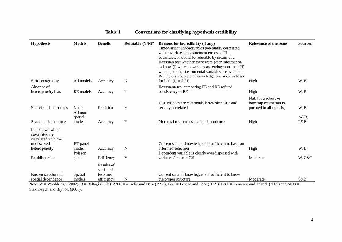
To classify for hypothesis credibility the state of practice on econometrics literature is taken as basis. This source provides guidance both on factors undermining credibility and on the relevance of incredibility (table 1).

Principles for overall classification

Three alternative (mutually exclusive) principles for overall classification were applied and had their results compared. The “only credibility matters” principle considers only the criteria of hypothesis credibility. The second principle is self-explained by its name which is “credibility and precision are equally important and prediction is irrelevant”. The third principle is “ladderwise” and establishes that “credibility matters most, followed by precision and then prediction”. The particular conventions adopted to operationalize the last two principles are omitted due to space limitations.

3.2 Models and estimator

3.2.1 General approach

The lack of knowledge regarding the predictors of Amazon fires requires an empirical approach which is both cautious and comprehensive. The process through which potentially relevant social and environmental attributes drive, or influence, the observed fire levels, has temporal and spatial dimensions, as previous sections suggest. It is also necessary to account for specific characteristics of the observation units, which are immutable at least within the period of analysis. A general and very simplistic model would be:

Yit = f(Xit1,…,XitK;Y-it) + uit (1.a)

6

uit = μi + vit (1.b)

With Yit ≡ fires detected at the i-th locality at the t-th time period, f(.) a functional form approximating the true form of E[Yit|Xit1,…,XitK; Y-it] and uit capturing unobservable fire predictors. The spatial dimension is introduced by the predictor Y-it, the fire level on other, presumably proximate, localities. The term μi captures time-invariant unobservables potentially correlated with covariates; it is also referred to as “non-observable heterogeneity”.

To account for spatial dependency of unobservables equation (1.b) has to be replaced by u = 휌∑ 푤 푢 + μ + v (1.b’), with W being the spatial weights matrix and ρ the parameter that measures the strength of neighborhood (or spill-over) effects.

3.2.2 Panel data models

Three classes of models are estimated, fixed-effects (within), random effects and a Hausman-Taylor instrumental-variable model (HT). Estimation of the first two reveals that some of the covariates are correlated with the unobserved heterogeneity and, therefore, RE results are unreliable due to inconsistency. The HT model is used to perform consistent estimation of coefficients of both time-variant and time-invariant covariates (Baltagi, 2001, chap.2, Hausman and Taylor, 1981).

The HT model is consistent only if based in the knowledge of which covariates are and are not correlated with the unobserved heterogeneity. This is the main weakness of HT model as the knowledge required is unavailable. Nevertheless, a tentative estimation is pursued by conjecturing that the unobserved heterogeneity captures how municipalities idiossincratically estimate the expected damage caused by accidental (unintended/scaped) fires, one of the main externalities of agricultural (intended) fires (Bowman et al., 2008). The rationale is simple. The probability of accidental fires is a function of socioeconomic observables and also of biophysical-climate factors whose variation is not completely observable due to limitations of spatial and temporal resolution (Cano-Crespo et al., 2015). This non-observed variation may be relevant across municipalities. In complement, the size of damage depends on the spatial distribution of tangibles within municipalities, which is not observed and may also vary across them.

With this reasoning, endogenous covariates are those related with the subjective expectations of accidental fire damage, what is, however, not completely clear. Seeking to perform a tentative estimation, the endogenous covariates were selected as detailed below.

Soybean and pasture areas: proxy for tangibles with a relevant degree of vulnerability to fire; GDP, HDI: proxy for the capacity to finance fire protection (Bowman et al., 2008); Rural settlements, protected areas (federal land): proxy for the size of damage bore by federal

government, which, therefore, does not falls upon municipalities; Precipitation: proxy for the contribution of climate to extinguish fires.

The previous discussion does not exclude the possibility that the unobservable and heterogeneous expected damage of accidental fires be time-variant. But it makes sense to believe that municipalities expectations are in some degree backward looking as the model behind tropical accidental fires remains obscure even for science, preventing full forward-looking behavior. Thus, municipal records of accidental fires may play a relevant role in defining the unobserved heterogeneity (Bowman et al., 2008). Of course the assumption that such records were not relevantly updated within the time horizon considered (2008-

7

2012) may be untrue as 2010 was a record year in fire detections (Marengo et al., 2011). Another reason why reliability of HT may be limited.

3.2.3 Count data models

The dependent variable is the count of fire detections, a natural number. However, linear models may return non-natural numbers as predictions. Results not subjected to this issue were generated by estimating Poisson and negative binomial models, which account for the binomial nature of the dependent variable (Cameron and Trivedi, 2009, Wooldridge, 2002).

3.2.4 Spatial panel models

Two families of spatial panels are estimated (econometric details are found in Millo and Piras, 2012). The first, hereafter referred as Baltagi-Elhorst (BE), assumes that the unobserved heterogeneity (μ) is not subjected to spatial dependence, i.e., the time-invariant relevant unobserved explanatories are not spatially correlated in a significant magnitude. The second family, Kapoor-Mutl-Pffafermayr (KMP) relaxes this assumption and therefore allows μ to be correlated within neighborhoods. Such extension adds larger generality to estimation as, a priori, there is no reason to believe that unobserved predictors of a spatially-dependent regressand are spatially independent. Spatial panel estimation is pursued with maximum likelihood (ML) and generalized method of moments (GMM) by relying on the R package “splm” by Millo and Piras (2012). The random-effects spatial panel could not be estimated with ML and only GMM estimation is reported.

8

Table 1 Conventions for classifying hypothesis credibility

Hypothesis Models Benefit Refutable (Y/N)? Reasons for incredibility (if any) Relevance of the issue Sources

Strict exogeneity All models Accuracy N

Time-variant unobservables potentially correlated with covariates: measurement errors on TI covariates. It would be refutable by means of a Hausman test whether there were prior information to know (i) which covariates are endogenous and (ii) which potential instrumental variables are available. But the current state of knowledge provides no basis for both (i) and (ii). High W, B

Absence of heterogeneity bias RE models Accuracy Y

Hausmann test comparing FE and RE refuted consistency of RE High W, B

Spherical disturbances None Precision Y Disturbances are commonly heteroskedastic and serially correlated

Null [as a robust or boostrap estimation is pursued in all models] W, B

Spatial independence

All non-spatial models Accuracy Y Moran's I test refutes spatial dependence High

A&B, L&P

It is known which covariates are correlated with the unobserved heterogeneity

HT panel model Accuracy N

Current state of knowledge is insufficient to basis an informed selection High W, B

Equidispersion Poisson panel Efficiency Y

Dependent variable is clearly overdispersed with variance / mean = 721 Moderate W, C&T

Known structure of spatial dependence

Spatial models

Results of statistical tests and efficiency N

Current state of knowlegde is insufficient to know the proper structure Moderate S&B

Note: W ≡ Wooldridge (2002), B ≡ Baltagi (2005), A&B ≡ Anselin and Bera (1998), L&P ≡ Lesage and Pace (2009), C&T ≡ Cameron and Trivedi (2009) and S&B ≡ Stakhovych and Bijmolt (2008).

9

4 Data 1

4.1 Price index

A crop price index was calculated as the weighted average of crop prices with weights given by crop’s share in total value of crop production. It were considered only the main crops in total harvested area of Legal Amazon, being them soy, rice, cassava, beans and maize. These crops corresponded to 87-88% of the regional total harvested area in 2008 and 2012. As the data is annually available, the index was calculated for the three years and then converted to the purchasing power of money of 2008. This was done for all monetary variables in the model (the remaining being municipal GDP and the value added by agriculture).

4.2 Temperature data

Land surface temperature, observed by satellite, was converted into intra-subannual statistics. The exam of the seasonal monthly pattern of temperature from 2003 to 2012 reveals the existence of two subannual periods which are most distinct in terms of temperature levels, being them January-June (wet season, Carmenta et al., 2013) and August-October (part of the dry season). Whole year averages would clearly eliminate subannual differences and thus destroy data variability. They are avoided in favour of two averages for each of the periods identified. It is based on these two intra-year averages that inter-year averages and standard deviations are calculated for the biannual periods of 2007-2008, 2009-2010 and 2011-2012. Each one represents, respectively, the state of temperature in 2008, 2010 and 2012. Additionally, the slope (or coefficient) of the deterministic trend for 2003-2012 was estimated by regressing the subannual averages against a regressor informing the years.

4.3 Soil

A soil map from IBGE for 2012 is used. Four main textures of soil were considered, loamy, clayey, high clayey and sandy. The municipal area with soils of non-identified texture and minor textures (organic and silty) are not considered for calculating the areal share of the four main textures. In fact, the shares reflect participation in the aggregated area of the four textures and, thus, one of the shares has to be left out of the models due to perfect collinearity. Loamy texture share was selected to be excluded.

4.4 Proxy for agricultural variables

Data on cattle prices is unavailable for most municipalities of Amazon, except for the ones belonging to Mato Grosso state. To fill this gap, two proxies are incorporated. The number of employment in beef processing industry, i.e., slaughterhouses and related meat activities, captures the part of demand cattle unrelated with dairy production. In complement, the size of the herd is a measure for cattle supply but also for productivity in ranching as the whole pasture areas of municipalities are controlled for. Value added by agriculture is also used as a proxy for productivity of the whole agricultural industry, i.e., crops and pasture.

4.5 Institutional variables

1 The detailed description of data sources is omitted due to data limitations.

10

As a proxy for environmental monitoring and control, the number of personnel working in local environmental department is used. The remaining institutional variables capture the extent of three modalities of federal lands, environmental protected areas, agrarian settlements of smallholders and indigenous lands. The three proxy the degree in which municipalities are monitored and control by federal government which is more financially able to develop such actions.

4.6 Economy and demography

Municipal GDP is a measure for the size of local economies and, together with population, introduces in the model the effect of per capital GDP. But also population also captures anthropic pressure especially because area of municipalities is controlled for, introducing the effect of population density. Head-count measures for poverty are also included, consisting in the share of households which, in the last census (of 2010), had income bellow one minimum wage2. What is introduced in the mode is the brake down of the share into four income levels, being them zero income, income of at most ¼ minimum wage / household/month, between ¼ and 1/2, and between ½ and 1 wage.

5 Results and discussion

5.1 MEP classification

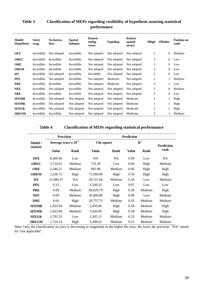
In terms of credibility of hypothesis, the main difference is between spatial and non-spatial models (table 3). However, in what regards to statistical performance, what matters most is whether MPEs belong to FE or RE families (table 4). In the latter aspect, high precision and high prediction accuracy are more recurrent among RE models. It makes sense to expect a worse prediction performance among FE as two of them (out of 6) do not estimate 15 (out of 49) coefficients of time-invariant covariates.

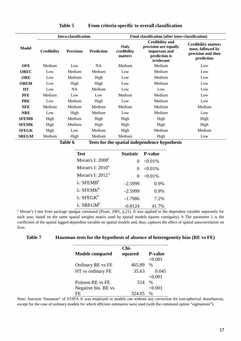
Of the three possible final classifications for MEPs (table 5), the one with higher level of discordance compared with others, “credibility and precision are equally important and prediction is irrelevant”, is supressed from analysis. Of the two remaining, it is opted for “credibility matters most, followed by precision and then prediction”, as it weights the three criteria more equally3.

In all three multicriteria classifications, only spatial models were high-ranked, mainly by not assuming incredible spatial independence (table 6). Even with a higher fraction of RE models exhibiting high precision and prediction accuracy, all RE models were low-ranked. This was mainly due to incredibility of the hypothesis of absence of correlation between covariates and the unobserved heterogeneity (see table 7). In contrast, only two of the six FE models were low-ranked, while the others were equally distributed in the medium and high ranks.

The HT model was low-ranked mainly due to the uncertainty regarding the definition of the set of endogenous covariates. It is important to notice that the non-acknowledgment of such reason for incredibility would not promote HT to the top level of the final rank due to the spatial independence assumption.

2Approximately U$300/household/month in values of 2010.

3 This seems subjective but it has a small effect as only 4 MPEs are differently classified in the two remaining final ranks (OFE, PFE, SFEGK, SREGM, table 5).

11

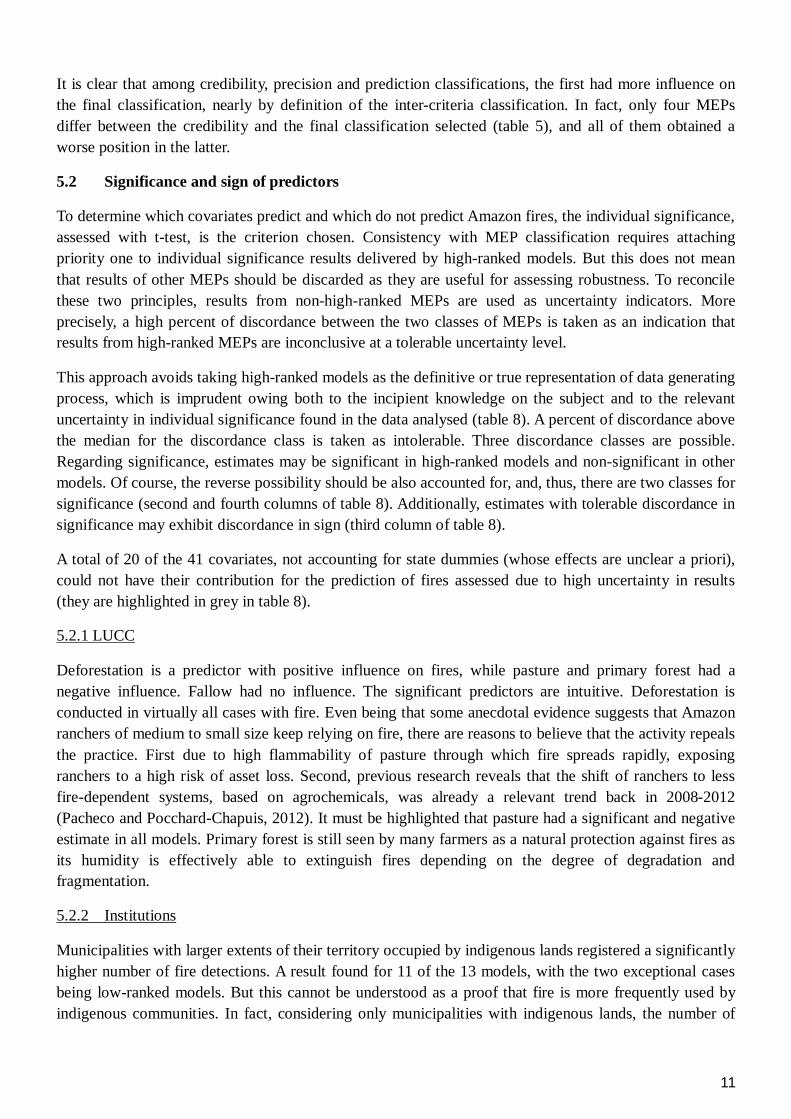
It is clear that among credibility, precision and prediction classifications, the first had more influence on the final classification, nearly by definition of the inter-criteria classification. In fact, only four MEPs differ between the credibility and the final classification selected (table 5), and all of them obtained a worse position in the latter.

5.2 Significance and sign of predictors

To determine which covariates predict and which do not predict Amazon fires, the individual significance, assessed with t-test, is the criterion chosen. Consistency with MEP classification requires attaching priority one to individual significance results delivered by high-ranked models. But this does not mean that results of other MEPs should be discarded as they are useful for assessing robustness. To reconcile these two principles, results from non-high-ranked MEPs are used as uncertainty indicators. More precisely, a high percent of discordance between the two classes of MEPs is taken as an indication that results from high-ranked MEPs are inconclusive at a tolerable uncertainty level.

This approach avoids taking high-ranked models as the definitive or true representation of data generating process, which is imprudent owing both to the incipient knowledge on the subject and to the relevant uncertainty in individual significance found in the data analysed (table 8). A percent of discordance above the median for the discordance class is taken as intolerable. Three discordance classes are possible. Regarding significance, estimates may be significant in high-ranked models and non-significant in other models. Of course, the reverse possibility should be also accounted for, and, thus, there are two classes for significance (second and fourth columns of table 8). Additionally, estimates with tolerable discordance in significance may exhibit discordance in sign (third column of table 8).

A total of 20 of the 41 covariates, not accounting for state dummies (whose effects are unclear a priori), could not have their contribution for the prediction of fires assessed due to high uncertainty in results (they are highlighted in grey in table 8).

5.2.1 LUCC

Deforestation is a predictor with positive influence on fires, while pasture and primary forest had a negative influence. Fallow had no influence. The significant predictors are intuitive. Deforestation is conducted in virtually all cases with fire. Even being that some anecdotal evidence suggests that Amazon ranchers of medium to small size keep relying on fire, there are reasons to believe that the activity repeals the practice. First due to high flammability of pasture through which fire spreads rapidly, exposing ranchers to a high risk of asset loss. Second, previous research reveals that the shift of ranchers to less fire-dependent systems, based on agrochemicals, was already a relevant trend back in 2008-2012 (Pacheco and Pocchard-Chapuis, 2012). It must be highlighted that pasture had a significant and negative estimate in all models. Primary forest is still seen by many farmers as a natural protection against fires as its humidity is effectively able to extinguish fires depending on the degree of degradation and fragmentation.

5.2.2 Institutions

Municipalities with larger extents of their territory occupied by indigenous lands registered a significantly higher number of fire detections. A result found for 11 of the 13 models, with the two exceptional cases being low-ranked models. But this cannot be understood as a proof that fire is more frequently used by indigenous communities. In fact, considering only municipalities with indigenous lands, the number of

12

fire detections is significantly higher in the outside of such lands compared with the inside, for the three years (p-value < 0.001%). Additionally, the relationship between share of indigenous lands in municipal area and fires in the outside of such lands seems to follow a curve with an “inverted-U” shape. Municipalities with a share above zero but below 50% register significantly (p-value < 5%) more fires than municipalities without indigenous lands. However, municipalities with an indigenous share of area above 50% do not significantly differ, in “outside fires”, from those without indigenous lands.

Indigenous lands function, in practice, as protected areas as they cannot be used by non-indigenous people and, thus, large scale deforesters are excluded (Nepstad et al., 2006). Considering this, the result found is perhaps an imprecise indication that indigenous lands may crowd-out fire use pushing fire density upward (fire/hectare) on the remaining area of municipalities4.

The fire crowd-out conjecture finds support in results of previous research, particularly those of Arima et al. (2011) and Nepstad et al. (2006). But specific cases and field evidence suggest a rather complex reality. In 2010, a drought year, a large scale fire occurred within the Xingú indigenous land at Mato Grosso state (Anderson et al., 2015). The same was observed during the 2005 drought in many locations of Acre state inhabited by traditional population5. The causes of fires remain unclear. One of the hypotheses on the table is that indigenous communities are facing challenges to adapt their fire use practices to the changing climate.

Anyhow, the result here found only shows that the municipal extent of indigenous lands predict fires. It supports no conclusion regarding underlying causalities. This is left for future research with proper causal inference methods.

5.2.3 Biophysical

Precipitation was not significantly correlated with fire, which may be due to imprecisions on the variables which only capture annual totalizations in the whole area of municipalities. Temperature had a significant role in predicting fires. Biannual standard deviations for one of the two subannual periods considered, the months of January-June, was significant in all models. The trend in temperature from 2003-2012, a crude proxy for the effect of climate change on temperature, was significant for the two subannual periods considered. Results thus indicate that both the increase in the level and uncertainty (volatility) of temperature may increase fires in Amazon, in line with recent climatologic and ecologic research (Vasconcelos et al., 2013).

The share of highly clayey soils, which are more fertile (Farella et al., 2007), were negatively correlated with fires. The reason for this result is unclear. Theoretically, land with higher potential profitability is more favourable to the accumulation of capital which is the means to finance shift to fire-free agriculture. But correlations of high clayey soils with fire-free soycrops and fallow-based agriculture are, respectively, negative and positive, refuting the potential explanation.

6 Conclusion

4 A precise indication would require a causal inference study for the impact of indigenous lands on fire detections but this is out of the scope of the paper.

5 Brown, Foster (University of Acre and Woods Hole Institute), personal communication.

13

Fire is one of the main threats for the conservation and development of Brazilian Amazon. Effective and efficient policy needs precise information and the paper provided a first step by building a dataset which is unparalleled in its geographical and temporal coverage.

The simple model selection procedure proposed is mainly targeted at forcing researchers to be clear about (i) actual small sample performance of models, (ii) the credibility of hypothesis assuring the desired small and large sample properties of estimators and (iii) the weight of the criteria (i) and (ii) in final decision.

Spatial fixed effects model proved best mainly for not relying on two assumptions refuted by the dataset, being them (i) spatial independence and (ii) lack of correlation between covariates and the unobserved heterogeneity.

Robustness was assessed with the discordance of models on significance and sign of coefficients. The result revealed intolerable uncertainty for 20 of 41 covariates. Of the remaining potential predictors, 12 were non-significant and 9 significant. Among the latter, three capture LUCC, one captures institutions, and the five remaining include temperature, soil texture and municipal area.

It was found evidence of indigenous lands crowding out fire as municipalities with larger extents of such lands also had higher fire counts. And, additionally, in most municipalities with indigenous lands, fire was concentrated in the outside of such lands. Both the level and volatility of temperature during January-June had positive influence on fire counts, in accordance with multiple studies predicting intensification of fires with climate change.

Multiple improvements of empirical analysis are possible and will be pursued in the near future. They comprise addition of (i) more precise precipitation metrics that capture inter-annual variability and also water deficit, (ii) cattle price, (iii) realistic transport cost metrics with intra-municipal variability, (iv) updated maps of indigenous land with precise dates of creation and ratification, (v) the year of 2014, for which LUCC data has become available during the final stage of paper preparation.

14

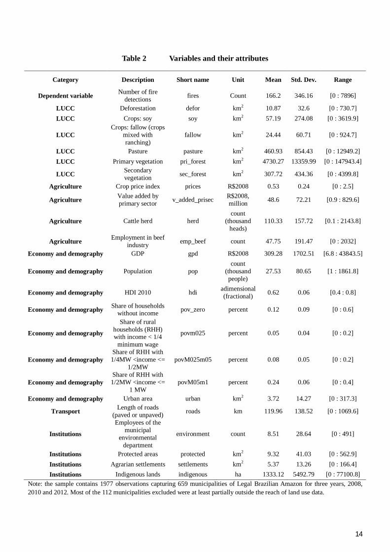
Table 2 Variables and their attributes

Category Description Short name Unit Mean Std. Dev. Range

Dependent variable Number of fire detections fires Count 166.2 346.16 [0 : 7896]

LUCC Deforestation defor km2 10.87 32.6 [0 : 730.7] LUCC Crops: soy soy km2 57.19 274.08 [0 : 3619.9]

LUCC Crops: fallow (crops

mixed with ranching)

fallow km2 24.44 60.71 [0 : 924.7]

LUCC Pasture pasture km2 460.93 854.43 [0 : 12949.2] LUCC Primary vegetation pri_forest km2 4730.27 13359.99 [0 : 147943.4]

LUCC Secondary vegetation sec_forest km2 307.72 434.36 [0 : 4399.8]

Agriculture Crop price index prices R$2008 0.53 0.24 [0 : 2.5]

Agriculture Value added by primary sector v_added_prisec R$2008,

million 48.6 72.21 [0.9 : 829.6]

Agriculture Cattle herd herd count

(thousand heads)

110.33 157.72 [0.1 : 2143.8]

Agriculture Employment in beef industry emp_beef count 47.75 191.47 [0 : 2032]

Economy and demography GDP gpd R$2008 309.28 1702.51 [6.8 : 43843.5]

Economy and demography Population pop count

(thousand people)

27.53 80.65 [1 : 1861.8]

Economy and demography HDI 2010 hdi adimensional (fractional) 0.62 0.06 [0.4 : 0.8]

Economy and demography Share of households without income pov_zero percent 0.12 0.09 [0 : 0.6]

Economy and demography

Share of rural households (RHH) with income < 1/4

minimum wage

povm025 percent 0.05 0.04 [0 : 0.2]

Economy and demography Share of RHH with 1/4MW <income <=

1/2MW povM025m05 percent 0.08 0.05 [0 : 0.2]

Economy and demography Share of RHH with 1/2MW <income <=

1 MW povM05m1 percent 0.24 0.06 [0 : 0.4]

Economy and demography Urban area urban km2 3.72 14.27 [0 : 317.3]

Transport Length of roads (paved or unpaved) roads km 119.96 138.52 [0 : 1069.6]

Institutions

Employees of the municipal

environmental department

environment count 8.51 28.64 [0 : 491]

Institutions Protected areas protected km2 9.32 41.03 [0 : 562.9] Institutions Agrarian settlements settlements km2 5.37 13.26 [0 : 166.4] Institutions Indigenous lands indigenous ha 1333.12 5492.79 [0 : 77100.8]

Note: the sample contains 1977 observations capturing 659 municipalities of Legal Brazilian Amazon for three years, 2008, 2010 and 2012. Most of the 112 municipalities excluded were at least partially outside the reach of land use data.

15

Table 2 Variables and their attributes (cont.)

Category Description Short name Unit Mean Std. Dev. Range

Biophysical Average annual precipitation: 2005-2008 and 2009-2012 av_ppt m/year 1.97 0.44 [0.9 : 3.5]

Biophysical SD annual precipitation: 2005-2008 and 2009-2012 sd_ppt m/year 0.27 0.18 [0 : 1.2]

Biophysical Precipitation: slope of

deterministic trend, 2003-2012

td_ppt m/year2 0 0.01 [-0.04:0.04]

Biophysical Average temperature,

january-june (JJ), current and previous year (CP)

av_temp_JJ K 301.85 2.81 [296.5 : 310]

Biophysical SD temperature, JJ, CP sd_temp_JJ K 3.05 2.28 [0 : 9.2]

Biophysical Slope of deterministic trend of temperature, 2003-2012, JJ td_temp_JJ K/year 0.01 0.06 [0.3 : 0.2]

Biophysical Average temperature, august-

october (AO), current and previous year (CP)

av_temp_AO K 305.41 4.18 [298.5 : 317.6]

Biophysical SD temperature, AO, CP sd_temp_AO K 2.98 2.2 [0 : 8.8]

Biophysical Slope of deterministic trend of temperature, 2003-2012,

AO td_temp_AO K/year 0.15 0.08 [0.2 : 0.4]

Biophysical Slope of the terrain, first quartile slope_p25 percent 0.01 0.01 [0.002;0.04]

Biophysical Slope of the terrain, second quartile slope_p50 percent 0.02 0.01 [0 : 0.1]

Biophysical Slope of the terrain, third quartile slope_p75 percent 0.04 0.02 [0 : 0.2]

Biophysical Soil quality: share of sandy

texture in municipal area with identified soil texture

soil_sandy binary 0.17 0.21 [0,1]

Biophysical Soil quality: share of area with clayey texture soil_clayey percent 0.25 0.23 [0 : 1]

Biophysical Soil quality: share of area with high clayey texture soil_hclayey percent 0.07 0.16 [0 : 1]

Additional controls Municipal area area km2 7271.11 14448.02 [148 : 159533.3] Additional controls 2010 dummy d_2010 binary 0.33 0.47 [0,1] Additional controls 2012 dummy d_2012 binary 0.33 0.47 [0,1] Additional controls State dummies (nine states) d_uf binary 0.08 0.27 [0,1]

16

Table 3 Classification of MEPs regarding credibility of hypothesis assuring statistical performance

Model/ Hypothesis

Strict exog.

No hetero. bias

Spatial indepen.

Known endog. covar.

Equidisp. Known spatial struct.

#High #Moder. Position on rank

OFE Incredible Not adopted Incredible Not adopted Not adopted Not adopted 2 0 Medium

OREC Incredible Incredible Incredible Not adopted Not adopted Not adopted 3 0 Low

ORE Incredible Incredible Incredible Not adopted Not adopted Not adopted 3 0 Low OREM Incredible Incredible Incredible Not adopted Not adopted Not adopted 3 0 Low HT Incredible Not adopted Incredible Incredible Not adopted Not adopted 3 0 Low

PFE Incredible Not adopted Incredible Not adopted Moderate Not adopted 2 1 Medium

PRE Incredible Incredible Incredible Not adopted Moderate Not adopted 3 1 Low

NFE Incredible Not adopted Incredible Not adopted Not adopted Not adopted 2 0 Medium

NRE Incredible Incredible Incredible Not adopted Not adopted Not adopted 3 0 Low

SFEMB Incredible Not adopted Not adopted Not adopted Not adopted Moderate 1 1 High

SFEMK Incredible Not adopted Not adopted Not adopted Not adopted Moderate 1 1 High

SFEGK Incredible Not adopted Not adopted Not adopted Not adopted Moderate 1 1 High

SREGM Incredible Incredible Not adopted Not adopted Not adopted Moderate 2 1 Medium

Table 4 Classification of MEPs regarding statistical performance

Model / statistic

Precision Prediction

Average trace x 10-3 Chi-square R2 Prediction

rank Value Rank Value Rank Value Rank

OFE 8,369.46 Low NA NA 0.09 Low NA OREC 3,734.02 Medium 732.30 Low 0.60 High Medium ORE 2,346.51 Medium 845.86 Medium 0.60 High High

OREM 2,336.73 High 71,094.98 High 0.59 High High HT 21,980.37 NA 26,721.64 Medium 0.26 Low Medium PFE 0.13 Low 1,549.23 Low 0.07 Low Low PRE 0.09 Medium 80,029.79 High 0.28 Medium High NFE 0.09 Medium 39,494.89 High 0.09 Low Medium NRE 0.04 High 28,757.73 Medium 0.35 Medium Medium

SFEMB 1,822.94 Medium 3,450.66 High 0.58 Medium High SFEMK 1,822.94 Medium 3,450.66 High 0.58 Medium High SFEGK 2,781.55 Low 2,305.15 Medium 0.53 Medium Medium SREGM 1,724.14 High 3,288.63 Medium 0.55 Medium Medium

Note: Only the classification on trace is decreasing in magnitude as the higher the trace, the lower the precision. “NA” stands for “not applicable”.

17

Table 5 From criteria-specific to overall classification

Model

Intra-classification Final classification (after inter-classification)

Credibility Precision Prediction Only

credibility matters

Credibility and precision are equally

important and prediction is

irrelevant

Credibility matters most, followed by precision and then

prediction

OFE Medium Low NA Medium Medium Low OREC Low Medium Medium Low Medium Low ORE Low Medium High Low Medium Low

OREM Low High High Low Medium Low HT Low NA Medium Low Low Low PFE Medium Low Low Medium Medium Low PRE Low Medium High Low Medium Low NFE Medium Medium Medium Medium Medium Medium NRE Low High Medium Low Medium Low

SFEMB High Medium High High High High SFEMK High Medium High High High High SFEGK High Low Medium High Medium Medium SREGM Medium High Medium Medium High Low

Table 6 Tests for the spatial independence hypothesis

Test Statistic P-value Moran's I: 2008a 0 <0.01% Moran's I: 2010a 0 <0.01% Moran's I: 2012 a 0 <0.01% λ: SFEMBb -2.5999 0.9% λ: SFEMKb -2.5999 0.9% λ: SFEGKb -1.7986 7.2% λ: SREGMb -0.8124 41.7%

a Moran’s I test from package spatgsa command (Pisati, 2001, p.21). It was applied to the dependent variable separately for each year, based on the same spatial weights matrix used by spatial models (queen contiguity). b The parameter λ is the coefficient of the spatial lagged dependent variable on spatial models and, thus, captures the effect of spatial autocorrelation on fires.

Table 7 Hausman tests for the hypothesis of absence of heterogeneity bias (RE vs FE)

Models compared Chi-squared P-value

Ordinary RE vs FE 465.89 <0.001%

HT vs ordinary FE 35.63 0.045

Poisson RE vs FE 514 <0.001%

Negative bin. RE vs FE 324.05

<0.001%

Note: function “hausman” of STATA ® was employed in models ran without any correction for non-spherical disturbances, except for the case of ordinary models for which efficient estimators were used (with the command option “sigmamore”).

18

Table 8 Models (%) in which estimate status differ from high-ranked models and status of covariates as predictors after accounting for uncertainty

Covariate / Status High-ranked: sig, others: non-sig

High-ranked: sig +/-, others: sig -/+

High-ranked: non-sig, others: sig

Is predictor (Y/N)? [sign]

defor 45% 0% NA Y[+] soy 73% NA NA Unknown

fallow NA NA 0% N pasture 9% 0% NA Y[-]

pri_forest 9% 0% NA Y[-] sec_forest 55% NA NA Unknown

prices NA NA 45% Unknown v_added_prisec 73% NA NA Unknown

herd 36% 27% NA Unknown emp_beef 55% NA NA Unknown

gpd NA NA 18% N pop NA NA 18% N hdi NA NA 0% N

pov_zero 82% NA NA Unknown povm025 NA NA 18% N

povM025m05 NA NA 9% N povM05m1 73% NA NA Unknown

urban 73% NA NA Unknown roads 64% NA NA Unknown

environment NA NA 9% N protected NA NA 27% Unknown

settlements NA NA 27% Unknown indigenous 18% 0% NA Y[+]

av_ppt NA NA 0% N sd_ppt NA NA 18% N td_ppt NA NA 0% N

av_temp_JJ NA NA 36% Unknown sd_temp_JJ 0% 0% NA Y[+] td_temp_JJ 36% 0% NA Y[+]

av_temp_AO NA NA 45% Unknown sd_temp_AO NA NA 73% Unknown td_temp_AO 36% 0% NA Y[+]

slope_p25 73% NA NA Unknown slope_p50 64% NA NA Unknown slope_p75 73% NA NA Unknown soil_sandy NA NA 9% N soil_clayey NA NA 0% N

soil_hclayey 36% 0% NA Y[-] area 27% 0% NA Y[+]

d_2010 NA NA 64% Unknown d_2012 27% 9% NA Unknown

Note: detailed results are omitted due to space limitations.

19

7 References

Anderson, L. O., Aragão, L. E., Gloor, M., Arai, E., Adami, M., Saatchi, S. S., ... & Duarte, V. (2015). Disentangling the contribution of multiple land covers to fire-mediated carbon emissions in Amazonia during the 2010 drought. Global Biogeochemical Cycles, 29(10), 1739-1753.

Anselin, L., & Bera, A. K. (1998). Spatial dependence in linear regression models with an introduction to spatial econometrics. Statistics Textbooks and Monographs, 155, 237-290.

Arima, E. Y., Richards, P., Walker, R., Caldas, M. M., 2011. Statistical confirmation of indirect land use change in the Brazilian Amazon. Environmental Research Letters, 6(2), 024010.

Baltagi, B. (2008). Econometric analysis of panel data. John Wiley & Sons.

Barlow, J., Lennox, G. D., Ferreira, J., Berenguer, E., Lees, A. C., Mac Nally, R., ... & Parry, L. (2016). Anthropogenic disturbance in tropical forests can double biodiversity loss from deforestation. Nature, 535(7610), 144-147.

Betts, R. A., Malhi, Y., & Roberts, J. T. (2008). The future of the Amazon: new perspectives from climate, ecosystem and social sciences. Philosophical Transactions of the Royal Society of London B: Biological Sciences, 363(1498), 1729-1735.

Bowman, M. S., Amacher, G. S.,Merry, F. D., 2008. Fire use and prevention by traditional households in the Brazilian Amazon. Ecological Economics 67 (2008) 117 – 130.

Cameron, A. C., & Trivedi, P. K. (2009). Microeconometrics using stata (Vol. 5). College Station, TX: Stata press.

Cano-Crespo, A., Oliveira, P. J., Boit, A., Cardoso, M., & Thonicke, K. (2015). Forest edge burning in the Brazilian Amazon promoted by escaping fires from managed pastures. Journal of Geophysical Research: Biogeosciences, 120(10), 2095-2107.

Cardoso, M. F., Hurtt, G. C.,Moore, B., Nobre, C. A., & Prins, E. M. (2003). Projecting future fire activity in Amazonia. Global Change Biology, 9(5), 656-669.

Carmenta, R., Vermeylen, S., Parry, L., & Barlow, J. (2013). Shifting cultivation and fire policy: insights from the Brazilian Amazon. Human ecology, 41(4), 603-614.

Farella, N., Davidson, R., Lucotte, M., & Daigle, S. (2007). Nutrient and mercury variations in soils from family farms of the Tapajós region (Brazilian Amazon): recommendations for better farming. Agriculture, ecosystems & environment, 120(2), 449-462.

Godar, J., Gardner, T. A., Tizado, E. J., & Pacheco, P., 2014. Actor-specific contributions to the deforestation slowdown in the Brazilian Amazon. Proceedings of the National Academy of Sciences 111.43 (2014): 15591-15596.

Hargrave, J., & Kis-Katos, K. (2013). Economic causes of deforestation in the Brazilian Amazon: a panel data analysis for the 2000s. Environmental and Resource Economics, 54(4), 471-494.

Hausman, J. A., & Taylor, W. E. (1981). Panel data and unobservable individual effects. Econometrica: Journal of the Econometric Society, 1377-1398.

Kato, M. D. S., Kato, O. R., Denich, M., & Vlek, P. L. (1999). Fire-free alternatives to slash-and-burn for shifting cultivation in the eastern Amazon region: the role of fertilizers. Field crops research, 62(2), 225-237.

20

Leonel, M. (2000). O uso do fogo: o manejo indígena e a piromania da monocultura. Estudos Avançados, 14(40), 231-250.

LeSage,J., Pace, R. K., 2009. Introduction to Spatial Econometrics. CRC Press, Taylor & Francis.

Manski, C. F. (2003). Partial identification of probability distributions. Springer Science & Business Media.

Marchand, S. (2012). The relationship between technical efficiency in agriculture and deforestation in the Brazilian Amazon. Ecological Economics, 77, 166-175.#

Marengo, J. A., Tomasella, J., Alves, L. M., Soares, W. R., & Rodriguez, D. A. (2011). The drought of 2010 in the context of historical droughts in the Amazon region. Geophysical Research Letters, 38(12).

Millo, G., & Piras, G. (2012). splm: Spatial panel data models in R. Journal of Statistical Software, 47(1), 1-38.

Nepstad, D., Schwartzman, S., Bamberger, B., Santilli, M., Ray, D., Schlesinger, P., ... & Rolla, A. (2006). Inhibition of Amazon deforestation and fire by parks and indigenous lands. Conservation Biology, 20(1), 65-73.

Nepstad, D. C., AG Alencar, A. A., Schwartzman, S. C., J Nepstad, D. C., Schwartzman, S.P. (1999). Flames in the rain forest: origins, impacts and alternatives to Amazonian fires (No. 634.9618 N442). Pilot Program to Conserve the Brazilian Rain Forest, Brasilia (Brasil).

Pacheco, P., & Poccard-Chapuis, R. (2012). The complex evolution of cattle ranching development amid market integration and policy shifts in the Brazilian Amazon. Annals of the Association of American Geographers, 102(6), 1366-1390.

Pisati, M. (2001). sg162: tools for spatial data analysis. Stata Technical Bulletin, 60, 21-37.

Stakhovych, S., & Bijmolt, T. H. (2009). Specification of spatial models: A simulation study on weights matrices. Papers in Regional Science, 88(2), 389-408.

Vasconcelos, S. S., Fearnside, P. M., de Alencastro Graça, P. M. L., Dias, D. V., & Correia, F. W. S., 2013. Variability of vegetation fires with rain and deforestation in Brazil's state of Amazonas. Remote Sensing of Environment, 136, 199-209.

Wooldridge Jeffrey, M. (2002). Econometric analysis of cross section and panel data. Cambridge, MA: Massachusetts Institute of Technology.