PreconditioningTechniquesBasedonthe Birkhoff…benzi/Web_papers/bu17.pdf ·...

Comput. Methods Appl. Math. 2016; 17 (2):201–215

Research Article

Michele Benzi* and Bora Uçar

Preconditioning Techniques Based on theBirkhoff–von Neumann DecompositionDOI: 10.1515/cmam-2016-0040Received October 26, 2016; accepted November 14, 2016

Abstract:We introduce a class of preconditioners for general sparsematrices based on the Birkhoff–von Neu-mann decomposition of doubly stochastic matrices. These preconditioners are aimed primarily at solvingchallenging linear systems with highly unstructured and indefinite coefficient matrices. We present sometheoretical results and numerical experiments on linear systems from a variety of applications.

Keywords: Preconditioning, Parallel Computing, Doubly Stochastic Matrix, Bipartite Graphs, Birkhoff–von Neumann Decomposition

MSC 2010: 65F35, 65F08, 65F50, 65Y05, 15B51, 05C70

1 IntroductionWe consider the solution of linear systems Ax = b where A = [aij] ∈ ℝn×n, b is a given vector and x is the un-known vector. Our aim is to develop and investigate preconditioners for Krylov subspacemethods for solvingsuch linear systems, where A is highly unstructured and indefinite.

For a givenmatrix A, we first preprocess it to get a doubly stochasticmatrix (whose row and column sumsare one). Then using this doubly stochastic matrix, we select some fraction of some of the nonzeros of A tobe included in the preconditioner. Our main tools are the well-known Birkhoff–von Neumann (BvN) decom-position (this will be discussed in Section 2 for completeness) and a splitting of the input matrix in the formA = M − N based on its BvN decomposition. When such a splitting is defined, M−1 or solvers for My = z arerequired.We discuss sufficient conditions when such a splitting is convergent and discuss specialized solversfor My = z when these conditions are met. We discuss how to build preconditioners meeting the sufficiencyconditions. In case the preconditioners become restrictive in practice, their LU decomposition can be used.Our motivation is that the preconditioner M−1 can be applied to vectors via a number of highly concurrentsteps, where the number of steps is controlled by the user. Therefore, the preconditioners (or the splittings)can be advantageous for use in many-core computing systems. In the context of splittings, the application ofN to vectors also enjoys the same property. Thesemotivations are shared by recent work on ILU precondition-ers, where their fine-grained computation [9] and approximate application [2] are investigated for GPU-likesystems.

The paper is organized as follows. We first give necessary background (Section 2) on doubly stochasticmatrices and the BvN decomposition. We then develop splittings for doubly stochastic matrices (Section 3),where we analyze convergence properties and discuss algorithms to construct the preconditioners. Later inthe same section, we discuss how the preconditioners can be used for arbitrary matrices by some preprocess-ing. Here our approach results in a generalization of the Birkhoff–von Neumann decomposition for matriceswith positive and negative entries where the sum of the absolute values of the entries in any given row or

*Corresponding author: Michele Benzi: Department of Mathematics and Computer Science, Emory University, Atlanta, USA,e-mail: [email protected] Uçar: LIP, UMR5668 (CNRS – ENS Lyon – UCBL – Université de Lyon – INRIA), Lyon, France, e-mail: [email protected]

Authenticated | [email protected] author's copyDownload Date | 3/28/17 4:01 PM

202 | M. Benzi and B. Uçar, Preconditioning with the BvN Decomposition

column is one. This generalization could be of interest in other areas. Then, we give experimental results(Section 4) with nonnegative and also arbitrary matrices, and then conclude the paper.

2 Background and DefinitionsHere we define several properties of matrices: irreducible, full indecomposable, and doubly stochastic matri-ces. An n × n matrix A is reducible if there exists a permutation matrix P such that

PAPT = [A1,1 A1,2O A2,2

] ,

where A1,1 is an r × r submatrix, A2,2 is an (n − r) × (n − r) submatrix, and 1 ≤ r < n. If such a permutationmatrix does not exist, then A is irreducible [25, Chapter 1]. When A is reducible, either A1,1 or A2,2 can be re-ducible aswell, andwe can recursively identify their diagonal blocks, until all diagonal blocks are irreducible.That is, we can obtain

PAPT =[[[[[

[

A1,1 A1,2 ⋅ ⋅ ⋅ A1,s0 A2,2 ⋅ ⋅ ⋅ A2,s...

.... . .

...0 0 ⋅ ⋅ ⋅ As,s

]]]]]

]

,

where each Ai,i is square and irreducible. This block upper triangular form, with square irreducible diagonalblocks is called Frobenius normal form [19, p. 532].

An n × nmatrix A is fully indecomposable if there exists a permutationmatrix Q such that AQ has a zero-free diagonal and is irreducible [7, Chapters 3 and 4]. If A is not fully indecomposable, but nonsingular, itcan be permuted into the block upper triangular form

PAQT = [A1,1 A1,2O A2,2

] ,

where eachAi,i is fully indecomposable or canbe further permuted into the block upper triangular form. If thecoefficient matrix of a linear system is not fully indecomposable, the block upper triangular form should beobtained, and only the small systemswith the diagonal blocks should be factored for simplicity and efficiency[12, Chapter 6]. We therefore assume without loss of generality that matrix A is fully indecomposable.

An n × n matrix A is doubly stochastic if aij ≥ 0 for all i, j and Ae = ATe = e, where e is the vector ofall ones. This means that the row sums and column sums are equal to one. If these sums are less thanone, then the matrix A is doubly substochastic. A doubly stochastic matrix is fully indecomposable or isblock diagonal where each block is fully indecomposable. By Birkhoff’s theorem [4], there exist coefficientsα1, α2, . . . , αk ∈ (0, 1) with∑k

i=1 αi = 1, and permutation matrices P1, P2, . . . , Pk such that

A = α1P1 + α2P2 + ⋅ ⋅ ⋅ + αkPk . (1)

Such a representation of A as a convex combination of permutation matrices is known as a Birkhoff–vonNeumann decomposition (BvN); in general, it is not unique. TheMarcus–Ree theorem states that there are BvNdecompositions with k ≤ n2 − 2n + 2 for densematrices; Brualdi and Gibson [6] and Brualdi [5] show that fora fully indecomposable sparse matrix with τ nonzeros, we have BvN decompositions with k ≤ τ − 2n + 2.

An n × n nonnegative, fully indecomposable matrix A can be uniquely scaled with two positive diagonalmatrices R and C such that RAC is doubly stochastic [24].


M. Benzi and B. Uçar, Preconditioning with the BvN Decomposition | 203

3 Splittings of Doubly Stochastic Matrices

3.1 Definition and Properties

Let b ∈ ℝn be given and consider solving the linear system Ax = b where A is doubly stochastic. Hereafter weassume that A is invertible. After finding a representation of A in the form (1), pick an integer r between 1and k − 1 and split A as

A = M − N, (2)

whereM = α1P1 + ⋅ ⋅ ⋅ + αrPr , N = −αr+1Pr+1 − ⋅ ⋅ ⋅ − αkPk . (3)

Note that M and −N are doubly substochastic matrices.

Definition 1. A splitting of the form (2)withM andN given by (3) is said to be a doubly substochastic splitting.

Definition 2. A doubly substochastic splitting A = M − N of a doubly stochastic matrix A is said to bestandard if M is invertible. We will call such a splitting an SDS splitting.

In general, it is not easy to guarantee that a given doubly substochastic splitting is standard, except for sometrivial situation such as the case r = 1, in which case M is always invertible. We also have a characterizationfor invertible M when r = 2.

Theorem 1. LetM = α1P1 + α2P2. Then,M is invertible if (i) α1 ̸= α2, or (ii) α1 = α2 and all the fully indecom-posable blocks ofM have an odd number of rows (and columns). If any such block is of even order,M is singular.

Proof. We investigate the two cases separately.Case (i): Without loss of generality assume that α1 > α2. We have

M = α1P1 + α2P2 = P1(α1I + α2PT1P2).

The matrix α1I + α2PT1P2 is nonsingular. Indeed, its eigenvalues are of the form α1 + α2λj, where λj is thegeneric eigenvalue of the (orthogonal, doubly stochastic) matrix PT1P2, and since |λj| = 1 for all j and α1 > α2,it follows that α1 + α2λj ̸= 0 for all j. Thus, M is invertible.

Case (ii): This is a consequence of the Perron–Frobenius theorem. To see this, observe that we need toshow that under the stated conditions the sum P1 + P2 = P1(I + PT1P2) is invertible, i.e., λ = −1 cannot be aneigenvalue of PT1P2. Since both P1 and P2 are permutation matrices, PT1P2 is also a permutation matrix andthe Frobenius normal form T = Π(PT1P2)ΠT of P

T1P2, i.e., the block triangular matrix

T =[[[[[

[

T1,1 T1,2 ⋅ ⋅ ⋅ T1,s0 T2,2 ⋅ ⋅ ⋅ T2,s...

.... . .

...0 0 ⋅ ⋅ ⋅ Ts,s

]]]]]

]

,

has Ti,j = 0 for i ̸= j. The eigenvalues of PT1P2 are just the eigenvalues of the diagonal blocks Ti,i of T. Notethat there may be only one such block, corresponding to the case where PT1P2 is irreducible. Each diagonalblock Ti,i is also a permutation matrix. Thus, each Ti,i is doubly stochastic, orthogonal, and irreducible. Anymatrix of this kind corresponds to a cyclic permutation and has its eigenvalues on the unit circle. If a blockhas size r > 1, its eigenvalues are the pth roots of unity, εh, h = 0, 1, . . . , p − 1, with ε = e2πi/p, e.g., by thePerron–Frobenius theorem (see [17, p. 53]). But λ = −1 is a pth root of unity if and only if p is even. Since Mis a scalar multiple of P1 + P2 = P1(I + PT1P2), this concludes the proof.

Note that the fully indecomposable blocks ofM mentioned in the theorem are just connected components ofits bipartite graph.

It is possible to generalize the condition (i) in the previous theorem as follows.



Theorem 2. A sufficient condition forM = ∑ri=1 αiPi to be invertible is that one of the αi with 1 ≤ i ≤ r be greater

than the sum of the remaining ones.

Proof. Indeed, assuming (without loss of generality) that α1 > α2 + ⋅ ⋅ ⋅ + αr, we have

M = α1P1 + α2P2 + ⋅ ⋅ ⋅ + αrPr= P1(α1I + α2PT1P2 + ⋅ ⋅ ⋅ + αrP

T1Pr).

Thismatrix is invertible if andonly if thematrix α1I +∑ri=2 αiPT1Pi is invertible. Observing that the eigenvalues

λj of∑ri=2 αiPT1Pi satisfy

|λj| ≤ ‖α2PT1P2 + ⋅ ⋅ ⋅ + αrPT1Pr‖2 ≤

r∑i=2αi < α1

(where we have used the triangle inequality and the fact that the 2-norm of an orthogonal matrix is one), itfollows that M is invertible.

Again, this condition is only a sufficient one. It is rather restrictive in practice.

3.2 Convergence Conditions

Let A = M − N be an SDS splitting of A and consider the stationary iterative scheme

xk+1 = Hxk + c, H = M−1N, c = M−1b, (4)

where k = 0, 1, . . . and x0 is arbitrary. As iswell known, the scheme (4) converges to the solution of Ax = b forany x0 if and only if ρ(H) < 1. Hence, we are interested in conditions that guarantee that the spectral radiusof the iteration matrix

H = M−1N = −(α1P1 + ⋅ ⋅ ⋅ + αrPr)−1(αr+1Pr+1 + ⋅ ⋅ ⋅ + αkPk)

is strictly less than one. In general, this problem appears to be difficult. We have a necessary condition (The-orem 3), and a sufficient condition (Theorem 4) which is simple but restrictive.

Theorem 3. For the splitting A = M − N withM = ∑ri=1 αiPi andN = −∑

ki=r+1 αiPi to be convergent, it must hold

that∑ri=1 αi > ∑

ki=r+1 αi.

Proof. First, observe that since Pie = e for all i, both M and N have constant row sums:

Me =r∑i=1αiPie = βe, Ne = −

r∑i=1αiPie = (β − 1)e,

with β := ∑ri=1 αi ∈ (0, 1). Next, observe thatM−1Ne = λe is equivalent to Ne = λMe or, since we can assume

that λ ̸= 0, to Me = 1λNe. Substituting βe for Me and (β − 1)e for Ne, we find

βe = 1λ(β − 1)e or λ = β − 1

β.

Hence, β−1β is an eigenvalue of H = M−1N corresponding to the eigenvector e. Since |λ| = 1−ββ , we conclude

that ρ(H) ≥ 1 for β ∈ (0, 12 ]. This concludes the proof.

Theorem 4. Suppose that one of the αi appearing in M is greater than the sum of all the other αi. Thenρ(M−1N) < 1 and the stationary iterative method (4) converges for all x0 to the unique solution of Ax = b.

Proof. Assuming (without loss of generality) that

α1 > α2 + ⋅ ⋅ ⋅ + αk (5)

(which, incidentally, ensures that the matrix M is invertible), we show below that

‖H‖2 = ‖(α1P1 + ⋅ ⋅ ⋅ + αrPr)−1(αr+1Pr+1 + ⋅ ⋅ ⋅ + αkPk)‖2 < 1. (6)



This, together with the fact that ρ(H) ≤ ‖H‖2, ensures convergence. To prove (6) we start by observing that

M = α1P1 + ⋅ ⋅ ⋅ + αrPr = α1P1(I +α2α1Q2 + ⋅ ⋅ ⋅ +

αrα1Qr),

where Qi = PT1Pi. Thus, we have

M−1 = (α1P1 + ⋅ ⋅ ⋅ + αrPr)−1 =1α1

(I − G)−1PT1 ,

where we have definedG = − 1

α1

r∑i=2αiQi .

Next, we observe that ‖G‖2 < 1, since

‖G‖2 ≤1α1

r∑i=2αi‖Qi‖2 =

α2 + ⋅ ⋅ ⋅ + αrα1

< 1

as a consequence of (5). Hence, the expansion

(I − G)−1 =∞∑ℓ=0

Gℓ

is convergent, and moreover

‖(I − G)−1PT1‖2 = ‖(I − G)−1‖2 ≤

11 − ‖G‖2

≤1

1 − ( α2α1 + ⋅ ⋅ ⋅ +αrα1 )

.

The last inequality follows from the fact that ‖G‖2 ≤ ∑ri=2

αiα1 , as can be seen using the triangle inequality and

the fact that ‖Qi‖2 = 1 for all i = 2, . . . , r.Hence, we have

‖M−1N‖2 ≤1α1

11 − ( α2α1 + ⋅ ⋅ ⋅ +

αrα1 )

‖αr+1Pr+1 + ⋅ ⋅ ⋅ + αkPk‖2.

Using once again the triangle inequality (applied to the last term on the right of the foregoing expression),we obtain

‖M−1N‖2 ≤αr+1 + ⋅ ⋅ ⋅ + αk

α1 − (α2 + ⋅ ⋅ ⋅ + αr).

Using condition (5), we immediately obtain

αr+1 + ⋅ ⋅ ⋅ + αkα1 − (α2 + ⋅ ⋅ ⋅ + αr)

< 1,

therefore ‖M−1N‖2 < 1 and the iterative scheme (4) is convergent.

Note that if condition (5) is satisfied, then the value of r in (3) can be chosen arbitrarily; that is, the split-ting will converge for any choice of r between 1 and k. In particular, the splitting A = M − N with M = α1P1and N = −∑k

i=2 αiPi is convergent. It is an open question whether adding more terms to M (that is, usingM = ∑r

i=1 αiPi with r > 1) will result in a smaller spectral radius of H (and thus in faster asymptotic conver-gence); notice that adding terms to M will make application of the preconditioner more expensive.

Note that condition (5) is very restrictive. It implies that α1 > 12 , a very strong restriction. It is clear that

given a doubly substochastic matrix, in general it will have no representation (1) with α1 > 12 . On the other

hand, it is easy to find examples of splittings of doubly substochastic matrices for which α1 = 12 and the

splitting (3) with r = 1 is not convergent. Also, we have found examples with k = 3, r = 2 and α1 + α2 > α3where the splitting did not converge. It is an open problem to identify other, less restrictive conditions on theαi (with 1 ≤ i ≤ r) that will ensure convergence, where the pattern of the permutations could also be used.



3.3 Solving Linear Systems with M

The stationary iterations (4) for solving Ax = b or Krylov subspace methods using M as a preconditioner re-quire solving linear systems of the form Mz = y. Assume that M = α1P1 + α2P2 and α1 > α2. The stationaryiterations zk+1 = 1

α1 PT1 (y − α2P2zk) are convergent for any starting point, with the rate of α2

α1 . Therefore, ifM = α1P1 + α2P2 andM is as described in Theorem 1 (i), then we use the above iterations to applyM−1 (thatis, solve linear systems with M). If M is as described in Theorem 4, then we can still solve Mz = y by station-ary iterations, where we use the splitting M = α1P1 −∑k

r=2 αrPr. We note that application of ∑kr=2 αrPr to a

vector y, that is, z = (∑kr=2 αrPr)y, can be effectively computed in k − 1 steps, where at each step, we perform

z ← z + (αrPr)y. This last operation takes n input entries, scales them and adds them to n different positionsin z. As there are no read or write dependencies between these n operations, each step is trivially parallel; es-pecially in shared memory environments, the only parallelization overhead is the creation of threads. Eitherinput can be read in order, or the output can be written in order (by using the inverse of the permutation Pr).

As said before, splitting is guaranteed to work when α1 > 12 . Our experience showed that it does not work

in generalwhen α1 < 12 . Therefore,we suggest usingM as apreconditioner inKrylov subspacemethods. There

are two ways to do that. The first is to solve linear systems withM with a direct method by first factorizingM.Considering that the number of nonzeros in M would be much less than that of A, factorization of M couldbe much more efficient than factorization of A. The second alternative, which we elaborate in Section 3.4, isto build M in such a way that one of the coefficients is larger than the sum of the rest.

3.4 Algorithms for Constructing the Preconditioners

It is desirable to have a small number k in the Birkhoff–von Neumann decomposition while designing thepreconditioner. This is because of the fact that if we use splitting, then k determines the number of stepsin which we compute the matrix vector products. If we do not use all k permutation matrices, having a fewwith large coefficients should help to design the preconditioner. The problem of obtaining a Birkhoff–vonNeumann decomposition with the minimum number k is a difficult one, as pointed out by Brualdi [5] andhas been shown to be NP-complete [15]. This last reference also discusses a heuristic which delivers a smallnumber of permutation matrices. We summarize the heuristic in Algorithm 1.

Algorithm 1. A greedy heuristic for obtaining a BvN decomposition.Input: A, a doubly stochastic matrix;Output: a BvN decomposition (1) of A with k permutation matrices.(1) k ← 0(2) while (nnz(A) > 0)(3) k ← k + 1(4) Pk ← the pattern of a bottleneck perfect matching M in A(5) αk ← minMi,Pk(i)(6) A ← A − αkPk(7) endwhile

As seen in Algorithm 1, the heuristic proceeds step by step, where at each step j, a bottleneck matchingis found to determine αj and Pj. A bottleneck matching can be found using MC64 [13, 14]. In this heuristic,at line 4, M is a bottleneck perfect matching; that is, the minimum weight of an edge in M is the maximumamong all minimum elements of perfect matchings. Also, at line 5, αk is equal to the bottleneck value of theperfect matching M. A nice property of this heuristic is that it delivers αis in a non-increasing order; that isαj ≥ αj+1 for all 1 ≤ j < k. The worst case running time of a step of this heuristic can be bounded by the worstcase running time of a bottleneck matching algorithm. For matrices where nnz(A) = O(n), the best knownalgorithm is of time complexity O(n√n log n) (see [16]). We direct the reader to [8, p. 185] for other cases.



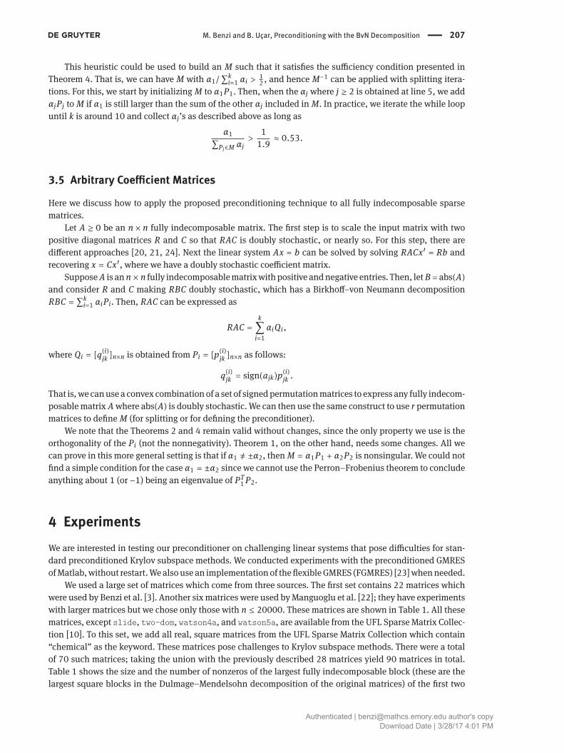
This heuristic could be used to build an M such that it satisfies the sufficiency condition presented inTheorem 4. That is, we can have M with α1/∑k

i=1 αi > 12 , and hence M

−1 can be applied with splitting itera-tions. For this, we start by initializingM to α1P1. Then, when the αj where j ≥ 2 is obtained at line 5, we addαjPj to M if α1 is still larger than the sum of the other αj included in M. In practice, we iterate the while loopuntil k is around 10 and collect αj’s as described above as long as

α1∑Pj∈M αj

>11.9 ≈ 0.53.

3.5 Arbitrary Coefficient Matrices

Here we discuss how to apply the proposed preconditioning technique to all fully indecomposable sparsematrices.

Let A ≥ 0 be an n × n fully indecomposable matrix. The first step is to scale the input matrix with twopositive diagonal matrices R and C so that RAC is doubly stochastic, or nearly so. For this step, there aredifferent approaches [20, 21, 24]. Next the linear system Ax = b can be solved by solving RACx� = Rb andrecovering x = Cx�, where we have a doubly stochastic coefficient matrix.

SupposeA is an n × n fully indecomposablematrixwithpositive andnegative entries. Then, letB = abs(A)and consider R and C making RBC doubly stochastic, which has a Birkhoff–von Neumann decompositionRBC = ∑k

i=1 αiPi. Then, RAC can be expressed as

RAC =k∑i=1αiQi ,

where Qi = [q(i)jk ]n×n is obtained from Pi = [p(i)jk ]n×n as follows:

q(i)jk = sign(ajk)p(i)jk .

That is,we canuse a convex combinationof a set of signedpermutationmatrices to express any fully indecom-posablematrix Awhere abs(A) is doubly stochastic. We can then use the same construct to use r permutationmatrices to define M (for splitting or for defining the preconditioner).

We note that the Theorems 2 and 4 remain valid without changes, since the only property we use is theorthogonality of the Pi (not the nonnegativity). Theorem 1, on the other hand, needs some changes. All wecan prove in this more general setting is that if α1 ̸= ±α2, thenM = α1P1 + α2P2 is nonsingular. We could notfind a simple condition for the case α1 = ±α2 since we cannot use the Perron–Frobenius theorem to concludeanything about 1 (or −1) being an eigenvalue of PT1P2.

4 ExperimentsWe are interested in testing our preconditioner on challenging linear systems that pose difficulties for stan-dard preconditioned Krylov subspace methods. We conducted experiments with the preconditioned GMRESofMatlab,without restart.Wealsouse an implementation of theflexibleGMRES (FGMRES) [23]whenneeded.

We used a large set of matrices which come from three sources. The first set contains 22 matrices whichwere used by Benzi et al. [3]. Another six matrices were used byManguoglu et al. [22]; they have experimentswith larger matrices but we chose only those with n ≤ 20000. These matrices are shown in Table 1. All thesematrices, except slide, two-dom, watson4a, and watson5a, are available from the UFL Sparse Matrix Collec-tion [10]. To this set, we add all real, square matrices from the UFL Sparse Matrix Collection which contain“chemical” as the keyword. These matrices pose challenges to Krylov subspace methods. There were a totalof 70 such matrices; taking the union with the previously described 28 matrices yield 90 matrices in total.Table 1 shows the size and the number of nonzeros of the largest fully indecomposable block (these are thelargest square blocks in the Dulmage–Mendelsohn decomposition of the original matrices) of the first two



matrix nA nnzA n nnz k

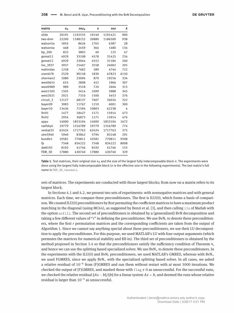
slide 20191 1192535 19140 1191421 900two-dom 22200 1188152 20880 1186500 938watson5a 1854 8626 1765 6387 28watson4a 468 2459 364 1480 134bp_200 822 3802 40 125 47gemat11 4929 33108 4578 31425 234gemat12 4929 33044 4552 31184 260lns_3937 3937 25407 3558 24002 205mahindas 1258 7682 589 4744 722orani678 2529 90158 1830 47823 6150sherman2 1080 23094 870 19256 334west0655 655 2808 452 1966 307west0989 989 3518 720 2604 315west1505 1505 5414 1099 3988 345west2021 2021 7310 1500 5453 376circuit_3 12127 48137 7607 34024 322bayer09 3083 11767 1210 6001 300bayer10 13436 71594 10803 62238 4lhr01 1477 18427 1171 15914 473lhr02 2954 36875 1171 15914 476appu 14000 1853104 14000 1853104 1672raefsky4 19779 1316789 19779 1316789 774venkat25 62424 1717763 62424 1717763 375utm5940 5940 83842 5794 83148 291bundle1 10581 770811 10581 770811 9508fp 7548 834222 7548 834222 8008dw8192 8192 41746 8192 41746 155FEM_3D 17880 430740 17880 430740 329

Table 1. Test matrices, their original size nA and the size of the largest fully indecomposable block n. The experiments weredone using the largest fully indecomposable block (n is the effective size in the following experiments). The last matrix’s fullname is FEM_3D_thermal1.

sets of matrices. The experiments are conducted with those largest blocks; from now on a matrix refers to itslargest block.

In Sections 4.1 and 4.2, we present two sets of experiments: with nonnegative matrices and with generalmatrices. Each time, we compare three preconditioners. The first is ILU(0), which forms a basis of compari-son.We created ILU(0) preconditioners byfirst permuting the coefficientmatrices to have amaximumproductmatching in the diagonal (using MC64), as suggested by Benzi et al. [3], and then calling ilu of Matlab withthe option nofill. The second set of preconditioners is obtained by a (generalized) BvN decomposition andtaking a few different values of “r” in defining the preconditioner. We use BvNr to denote these precondition-ers, where the first r permutation matrices and the corresponding coefficients are taken from the output ofAlgorithm 1. Since we cannot say anything special about these preconditioners, we use their LU decomposi-tion to apply the preconditioner. For this purpose, we used MATLAB’s LU with four output arguments (whichpermutes the matrices for numerical stability and fill-in). The third set of preconditioners is obtained by themethod proposed in Section 3.4 so that the preconditioners satisfy the sufficiency condition of Theorem 4,and hence we can use the splitting based specialized solver. We use BvN∗ to denote these preconditioners. Inthe experiments with the ILU(0) and BvNr preconditioners, we used MATLAB’s GMRES, whereas with BvN∗

we used FGMRES, since we apply BvN∗ with the specialized splitting based solver. In all cases, we askeda relative residual of 10−6 from (F)GMRES and run them without restart with at most 3000 iterations. Wechecked the output of (F)GMRES, and marked those with flag ̸= 0 as unsuccessful. For the successful runs,we checked the relative residual ‖Ax − b‖/‖b‖ for a linear system Ax = b, and deemed the runs whose relativeresidual is larger than 10−4 as unsuccessful.



(a) Nonnegative matrices (b) General matrices

Figure 1. Performance profiles for the number of iterations with ILU(0), BvNr with r = 2, 4, 8, and BvN∗.

4.1 Nonnegative Matrices

The first set of experiments is conducted on nonnegativematrices. Let A be amatrix from the data set (Table 1and another 62 matrices) and B = abs(A), that is, bij = |aij|. We scaled B to a doubly stochastic form with themethod of Knight and Ruiz [20]. We asked a tolerance of 10−8 (so that row and column sums can deviatefrom 1 by 10−8). We then obtained the Birkhoff–von Neumann decomposition by using Algorithm 1. Whenthe bottleneck value found at a step was smaller than 10−10, we stopped the decomposition process – hencewe obtain an “approximate” Birkhoff–vonNeumann decomposition of an “approximately” doubly stochasticmatrix. Thiswaywe obtained B ≈ α1P1 + α2P2 + ⋅ ⋅ ⋅ + αkPk. Then, let x⋆ be a randomvectorwhose entries arefrom the uniform distribution on the open interval (0, 1), generated using rand of Matlab. We then definedb = Bx⋆ to be the right-hand side of Bx = b.

We report our experiments with GMRES and FGMRES using different permutation matrices on nonnega-tivematrices inTable2. Thefirst part of the table gives thenumber ofGMRES iterationswith the ILU(0) precon-ditioner, and with the proposed Birkhoff–von Neumann based preconditioner, using r = 1, 2, 4, 8, 16, 32,and 64 permutation matrices and their coefficients. When there were less than r permutation matrices in theBvN decomposition, we used all available permutation matrices. Note that this does not mean that we havean exact inverse, as the BvN decomposition is only approximative. We also report results with FGMRES forthe BvN∗ preconditioners. For this case, we give the number r of permutation matrices used and the numberof FGMRES iterations (under the column “it”). In the second part (the last row of the table), we give the num-ber of successful runs with different preconditioners; here we also give the average number of permutationmatrices in BvN∗ under the column “r”.

Some observations are in order. As seen in Table 2, ILU(0) results in 11 successful runs on the matriceslisted in the first part of the table, and 32 successful runs in all 90 matrices. BvNr preconditioners with dif-fering number of permutationmatrices result in at least 53 successful runs in total, where BvN∗ obtained thehighest number of successful runs, but it has in only a few cases the least number of iterations. In 20 cases inthe first part of the table, we see that adding more permutation matrices usually helps in reducing the num-ber of iterations. This is not always the case though. We think that this is due to the preconditioner becomingbadly conditionedwith the increasing number of permutationmatrices; if we use the full BvNdecomposition,we will have the same conditioning as in A.

In order to clarify more, we present the performance profiles [11] for ILU(0), BvNr with r = 2, 4, 8, andBvN∗ in Figure 1a. A performance profile for a preconditioner shows the fraction of the test cases inwhich thenumber of (F)GMRES iterations with the preconditioner is within τ times the smallest number of (F)GMRESiterations observed (with thementioned set of preconditioners). Therefore, the higher the profile of a precon-ditioner, the better is its performance. As seen in this figure, BvN∗ and BvN8 manifest themselves as the bestpreconditioners; they are better than others after around τ = 1.1, while BvN8 being always better than others.



BvNr (iterations) BvN∗

matrix ILU(0) 1 2 4 8 16 32 64 r it.

slide – 1102 1158 946 787 567 566 131 10 884two-dom 1328 – – – 2774 2088 1719 1429 – –watson5a – 453 516 610 806 908 908 908 5 621watson4a 49 146 133 139 124 93 32 5 12 129bp_200 – 36 26 25 12 7 3 3 8 25gemat11 176 – – 2857 2118 1406 664 169 – –gemat12 263 – – 2906 2237 1591 – 145 – –lns_3937 349 2067 1286 666 229 56 14 5 10 1138mahindas – 303 283 245 173 87 40 21 7 278orani678 – 371 360 334 303 283 264 221 5 335sherman2 19 324 238 157 96 51 21 7 9 235west0655 71 331 275 188 139 – – 31 9 270west0989 – 194 167 114 63 35 19 9 8 165west1505 – 335 254 166 91 49 27 10 9 241west2021 – 406 323 217 – 47 34 13 8 315circuit_3 – – – – – – – 1426 – –bayer09 124 521 434 291 204 110 28 7 7 393bayer10 – – – – – – – – – –lhr01 – 574 350 216 130 86 42 18 7 313lhr02 – 565 351 219 136 87 45 19 8 314appu 31 50 50 52 56 62 74 82 7 50raefsky4 – – 2728 2735 2444 1559 1739 1230 6 2370venkat25 – – – – – – – – – –utm5940 – 2633 2115 – – – 153 34 7 2069bundle1 25 163 150 139 149 174 158 139 5 149fp – – – – – – – – – –dw8192 – – – 2398 1516 650 81 8 – –FEM_3D 7 37 35 38 72 58 25 6 9 33

Number of successful runs with all 90 matrices

32 58 71 60 57 53 58 61 7 77

Table 2. The number of GMRES iterations with ILU(0) and BvNr with different number of permutation matrices, and the numberof permutation matrices and FGMRES iterations with BvN∗. (F)GMRES are run with tolerance 10−6, without restart and with atmost 3000 iterations. The symbol “–” flags the cases where (F)GMRES were unsuccessful. All matrices are nonnegative.

BvN∗ is a little behind ILU(0) at the beginning but then catches up with BvN8 at around 1.2 and finishes asthe best alternative.

Although we are mostly concerned with robustness of the proposed preconditioners and their potentialfor parallel computing, we give a few running time results on a sequential Matlab environment (on a core ofan Intel Xeon E5-2695with 2.30 GHz clock speed). We present the complexity of the preconditioners and therunning time of (F)GMRES (total time spent in the iterations) for the cases where ILU(0) resulted in conver-gence in Table 3. This set of matrices is chosen to give the running time of (F)GMRES with all preconditionersunder study. Otherwise, it is not very meaningful to use sophisticated preconditioners when ILU(0) is effec-tive. Furthermore, the applications of ILU(0) and BvNr require triangular solves, which are efficiently imple-mented in MATLAB. On the other hand, the application of BvN∗ requires permutations and scaling, whichshould be very efficient in parallel. The running time given in the right side of Table 3 should not be taken atface value. The complexities of BvNr are given as the ratio (nnz(L + U) − n)/nnz(A), where L and U are thefactors of the preconditioner. In this setting, ILU(0) has always a complexity of 1.0. The complexity of BvN∗

is given as nnz(M)/nnz(A). As seen in this table, the LU-factors of BvNr with r ≤ 8 have reasonable numberof nonzeros; the complexity of the preconditioners is less than one in all cases except two-dom, lns_3937,west0655, and appu. In some preliminary experiments, we have seen large numbers when r ≥ 16. This wasespecially important for appu where the full LU factorization of A contained 85.67 ⋅ nnz(A) nonzeros and M



Complexity of M Running time

BvNr BvNr

2 4 8 BvN∗ ILU(0) 2 4 8 BvN∗

two-dom 0.03 0.04 1.33 0.08 3219.99 – – 6108.59 –watson4a 0.28 0.36 0.44 0.66 0.06 0.24 0.26 0.21 6.99gemat11 0.23 0.35 0.65 0.61 8.31 – 851.16 458.18 –gemat12 0.21 0.31 0.58 0.61 10.93 – 825.32 492.63 –lns_3937 0.29 0.55 1.67 0.63 27.28 131.73 31.42 3.84 519.83sherman2 0.06 0.10 0.14 0.26 0.02 0.83 0.39 0.16 20.13west0655 0.42 0.69 1.11 0.62 0.08 0.94 0.46 0.26 16.84bayer09 0.32 0.52 0.91 0.51 0.41 2.89 1.34 0.70 42.96appu 0.01 0.02 7.05 0.04 1.59 1.07 1.18 3.13 31.99bundle1 0.01 0.01 0.02 0.03 0.94 4.70 4.13 4.31 88.82FEM_3D 0.05 0.08 0.78 0.27 0.36 0.73 0.83 2.23 23.40

Table 3. The complexity of the preconditioners and the running time of the solver. The complexities of BvNr are given as theratio (nnz(L + U) − n)/ nnz, where L and U are the factors of the preconditioner (ILU(0) has a complexity of 1.0), and that ofBvN∗ is given as nnz(M)/ nnz(A). A sign of “–” in the running time column flags the cases where (F)GMRES were unsuccessful.All matrices are nonnegative.

suffered large fill-in. We run the solver with a large error tolerance of 1.0e-1, as this was enough to get theouter FGMRES to converge. The outer FGMRES iterations would change if a lower error tolerance is used inthe inner solver, but we do not dwell into this issue here. With the specified parameters, an application ofBvN∗ required, for the data shown in Table 3, between 128 and 162 iterations.

We now comment on the running time of the preconditioner set up phase. The first step is to apply thescalingmethod of Knight and Ruiz [20]. The dominant cost in this step is sparsematrix-vector and sparsema-trix transpose-vector multiply operations. The second step is to obtain a BvN decomposition, or a partial one,using the algorithms for the bottleneck matching problem from MC64 [13, 14]; these algorithms are highlyefficient. The number of sparse matrix-vector and sparse matrix transpose-vector multiply operations (MVP)in the scaling algorithm, the running time of the scaling algorithmwith the previous setting, and the runningtime of the partial BvN decomposition with 16 permutation matrices are shown for the same set of matricesin Table 4. Since an application of BvN∗ required between 128 and 162 iterations, and those iterations areno more costly than sparse matrix vector operations, we could relate the running time of FGMRES with BvN∗

in Table 3 to the scaling algorithm. For example, for lns_3937 a matrix vector multiplication should not costmore than 0.27/3732 seconds, while the application of BvN∗ required a total of 1138 ⋅ 152 steps of innersolver. In principle the total cost of the inner solver should be around 12.5, but in Table 3, we see 519.83 sec-onds of total FGMRES time. As seen in Table 4, for this set of matrices the scaling algorithm and the partialBvN decomposition algorithms are fast. There are efficient parallel scaling algorithms [1], and the one that weused [20] can also be efficiently parallelized by tapping into the parallel sparse matrix vector multiplicationalgorithms.

4.2 General Matrices

In this set of experiments, we used the matrices listed before, while retaining the sign of the nonzero entries.We used the same scaling algorithm as in the previous section and the proposed generalized BvN decomposi-tion (Section 3.5) to construct the preconditioners. As in the previous subsection, we report our experimentswith GMRES and FGMRES using different permutation matrices in Table 5. In particular, we report the num-ber of GMRES iterationswith the ILU(0) preconditioner, andwith the proposed Birkhoff–vonNeumann basedpreconditioner, using r = 1, 2, 4, 8, 16, 32, and 64 permutation matrices and their coefficients. We also re-port results with FGMRES for the BvN∗ preconditioners. Again, the number r of permutation matrices usedand the number of FGMRES iterations (under the column “it.”) are given for BvN∗. The last row of the ta-



running time (.s)

matrix MVP Scaling BvN

two-dom 438 0.67 3.03watson4a 40368 0.44 0.00gemat11 2286 0.28 0.04gemat12 843216 1.01 0.04lns_3937 3732 0.27 0.04sherman2 1966 0.06 0.01west0655 1846 0.03 0.00bayer09 3626 0.10 0.01appu 46 0.15 1.57bundle1 116 0.13 0.78FEM_3D_th 52 0.04 0.81

Table 4. The total number of sparse matrix-vector and sparse matrix transpose-vector multiply operations (MVP) in the scalingalgorithm, the running time of the scaling algorithm and the partial BvN decomposition algorithm in seconds.

BvNr it. BvN∗

matrix ILU(0) 1 2 4 8 16 32 64 r it.

slide 208 1051 999 745 685 490 783 659 10 663two-dom 149 579 553 – 610 607 432 360 7 573watson5a – 805 839 883 1094 1068 1068 1068 5 947watson4a 48 160 149 135 120 81 34 5 12 124bp_200 – 35 26 22 11 6 3 3 8 24gemat11 239 – – – 2486 1588 750 152 – –gemat12 344 – – – 2607 1615 – – – –lns_3937 134 1710 969 – 121 23 9 4 10 879mahindas – 259 232 180 121 51 – 12 7 232orani678 – 356 341 320 288 – 225 196 5 316sherman2 18 327 234 116 65 31 16 8 9 225west0655 50 298 229 164 101 64 30 – 9 222west0989 – 199 165 113 63 37 19 8 8 166west1505 – 343 262 170 92 49 27 12 9 256west2021 – 411 323 225 115 48 28 12 8 316circuit_3 – – – – – – – 1178 – –bayer09 39 312 193 105 58 – 11 5 7 213bayer10 – – 2624 2517 2517 2517 2517 2517 3 2594lhr01 – 495 314 – 117 65 28 14 7 279lhr02 – 508 315 – 119 67 28 15 8 277appu 31 50 50 52 56 62 74 82 7 51raefsky4 499 1207 722 472 592 403 860 617 6 656venkat25 163 – – 1863 – – 258 – 8 2493utm5940 – 1972 1588 1173 787 536 196 34 7 1520bundle1 18 130 123 115 127 137 129 102 5 125fp – – 2953 – – – 120 185 6 2779dw8192 – – – 2450 1536 661 82 11 – –FEM_3D 7 42 40 40 74 62 27 6 9 38

Number of successful runs with all 90 matrices

35 65 72 51 57 53 56 58 7 82

Table 5. The number of GMRES iterations with different number of permutation matrices in M with tolerance 10−6. We ranGMRES (without restart) for at most 3000 iterations; the symbol “–” flags cases where GMRES did not converge to therequired tolerance.Matrices have negative and positive entries.



Complexity of M Running time

BvNr BvNr

2 4 8 BvN∗ ILU(0) 2 4 8 BvN∗

slide 0.03 0.05 4.04 0.10 38.67 300.65 176.02 148.79 1017.34two-dom 0.03 0.04 1.31 0.08 56.40 183.60 – 205.53 1122.33watson4a 0.28 0.36 0.44 0.66 0.05 0.28 0.24 0.19 6.58gemat11 0.23 0.35 0.65 0.61 16.57 – – 1548.86 –gemat12 0.21 0.31 0.58 0.61 34.15 – – 1578.89 –lns_3937 0.29 0.55 1.66 0.63 4.68 186.25 – 3.12 359.80sherman2 0.06 0.10 0.14 0.26 0.02 0.80 0.25 0.09 18.03west0655 0.42 0.69 1.08 0.62 0.06 0.65 0.38 0.15 13.53bayer09 0.32 0.52 0.90 0.51 0.05 0.62 0.21 0.08 21.12appu 0.01 0.02 7.05 0.04 1.64 2.06 2.16 4.64 32.71raefsky4 0.02 0.02 0.29 0.07 206.02 262.48 116.39 182.10 1027.58venkat25 0.05 0.53 3.61 0.23 94.29 – 5462.64 – 20382.59bundle1 0.01 0.01 0.02 0.03 0.50 4.81 4.84 5.46 76.47FEM_3D 0.05 0.08 0.78 0.27 0.34 1.10 1.10 3.11 30.07

Table 6. The complexity of the preconditioners and the running time of the solver. The complexities of BvNr are given as the ra-tio (nnz(L + U) − n)/ nnz, where L and U are the factors of the preconditioner (ILU(0) has a complexity of 1.0), and that of BvN∗

is given as nnz(M)/ nnz(A). The symbol “–” in the running time column flags the cases where (F)GMRES were unsuccessful.Matrices have negative and positive entries.

ble gives the number of successful runs with different preconditioners in all 90 matrices; here the averagenumber of permutation matrices in BvN∗ is also given under the column “r”. We again use the performanceprofiles shown in Figure 1b to see the effects of the preconditioners. As seen in this table and the associatedperformance profile, the preconditioners behave much like they do in the nonnegative case. In particular,BvN∗ and BvN8 deliver the best performance in terms of number of iterations, followed by ILU(0).

We also give the complexity of the preconditioners and the running time of (F)GMRES (total time spentin the iterations) for the cases where ILU(0) resulted in convergence in Table 6. The complexities of the pre-conditioners remain virtually the same, as expected. As before, the running time is just to give a rough ideain a sequential MATLAB environment. We note that BvN∗ required, on average, between 125 and 151 inneriterations. Finally, note that nothing changes for the scaling and BvN decomposition algorithms with respectto the nonnegative case (Table 4 remains as it is for the general case).

4.3 Further Investigations

Here, we give some further experiments to shed light into the behavior of the proposed preconditioners. Wecompare BvN∗ with BvNr having the same number of permutation matrices. For this purpose, we created aBvN∗ preconditioner andused thenumber r of its permutationmatrices to create another preconditionerBvNrby just taking the first r permutationmatrices from aBvNdecomposition obtained byAlgorithm1. The resultsare shown in Table 7, where we give the sum of the coefficients used in constructing the preconditioners andthe number of (F)GMRES iterations for a subset of matrices from Table 6, where BvN∗ led to a short runningtime.

As seen in Table 7, BvNr has a larger sum of coefficients than BvN∗ with the same number r of permu-tation matrices. This is expected as Algorithm 1 finds coefficients in a non-increasing order; hence the first rcoefficients are the largest r ones. The number of (F)GMRES iterations is usually inversely proportional to thesum of the coefficients; a higher sum of coefficients usually results in a smaller number of iterations for thesame matrix.



∑ αi it.

matrix BvN∗ BvNr BvN∗ BvNr

watson4a 0.43 0.57 124 111lns_3937 0.29 0.80 881 68sherman2 0.24 0.61 226 59west0655 0.12 0.45 222 97bayer09 0.19 0.50 216 59appu 0.09 0.13 50 55bundle1 0.01 0.01 125 110FEM_3D 0.35 0.55 39 79

Table 7. Comparing BvN∗ with BvNr having the same number of permutation matrices in terms of the sum of the coefficient ofpermutation matrices and the number of (F)GMRES iterations (it.).Matrices have negative and positive entries.

5 Conclusions and Open QuestionsWe introduced a class of preconditioners for general sparsematrices based on the Birkhoff–vonNeumann de-composition of doubly stochastic matrices. These preconditioners are aimed primarily at solving challenginglinear systems with highly unstructured and indefinite coefficient matrices in parallel computing environ-ments. We presented some theoretical results and numerical experiments on linear systems from a variety ofapplications. We regard this work to be a proof of concept realization; many challenging questions remain tobe investigated to render the proposed preconditioners competitive with the standard approaches.

Based on our current theoretical findings,we suggest the use of proposed preconditionerswithin a Krylovsubspace method. There are two ways to go about this. In the first one, the preconditioners are built to sat-isfy a sufficiency condition that we identified (Theorem 4). This way, the application of the preconditionerrequires a small number of highly concurrent steps, where there is no data dependency within a step. In thesecond alternative, one obtains the LU decomposition of the preconditioners that are built arbitrarily. Here,the proposed preconditioner is therefore constructed as a complete factorization of an incompletematrix. Wedemonstrated that using around eight matrices is good enough for this purpose. Beyond that number, the LUdecomposition of the preconditioner can become a bottleneck (but remains always cheaper than that of theoriginal matrix). Is there a special way to order these preconditioners for smaller fill-in?

The construction of the preconditioners needs an efficient doubly stochastic scaling algorithm. Theknown algorithms for this purpose are iterative schemes whose computational cores are sparse matrix-vectormultiply operations whose efficient parallelization is well known. For constructing these preconditioners,we then need a bottleneck matching algorithm. The exact algorithms for this purpose are efficient on se-quential execution environments, but hard to parallelize efficiently. There are efficiently parallel heuristicsfor matching problems [18], and more research is needed to parallelize the heuristic for obtaining a BvNdecomposition while keeping an eye on the quality of the preconditioner.

Acknowledgment: We thank Alex Pothen for his contributions to this work. This work resulted from the col-laborative environment offered by the Dagstuhl Seminar 14461 on High-Performance Graph Algorithms andApplications in Computational Science (November 9–14, 2014).

Funding: The work of Michele Benzi was supported in part by NSF grant DMS-1418889. Bora Uçar was sup-ported in part by French National Research Agency (ANR) project SOLHAR (ANR-13-MONU-0007).



References[1] P. R. Amestoy, I. S. Duff, D. Ruiz and B. Uçar, A parallel matrix scaling algorithm, in: High Performance Computing for Com-

putational Science – VECPAR 2008, Lecture Notes in Comput. Sci. 5336, Springer, Berlin (2008), 301–313.[2] H. Anzt, E. Chow and J. Dongarra, Iterative sparse triangular solves for preconditioning, in: Euro-Par 2015: Parallel Pro-

cessing, Lecture Notes in Comput. Sci. 9233, Springer, Berlin (2015), 650–651.[3] M. Benzi, J. C. Haws and M. Tuma, Preconditioning highly indefinite and nonsymmetric matrices, SIAM J. Sci. Comput. 22

(2000), no. 4, 1333–1353.[4] G. Birkhoff, Tres observaciones sobre el algebra lineal, Univ. Nac. Tucumán Rev. Ser. A 5 (1946), 147–150.[5] R. A. Brualdi, Notes on the Birkhoff algorithm for doubly stochastic matrices, Canad.Math. Bull. 25 (1982), no. 2,

191–199.[6] R. A. Brualdi and P. M. Gibson, Convex polyhedra of doubly stochastic matrices. I: Applications of the permanent function,

J. Combin. Theory Ser. A 22 (1977), no. 2, 194–230.[7] R. A. Brualdi and H. J. Ryser, Combinatorial Matrix Theory, Encyclopedia Math. Appl. 39, Cambridge University Press,

Cambridge, 1991.[8] R. Burkard, M. Dell’Amico and S. Martello, Assignment Problems, SIAM, Philadelphia, 2009.[9] E. Chow and A. Patel, Fine-grained parallel incomplete LU factorization, SIAM J. Sci. Comput. 37 (2015), no. 2,

C169–C193.[10] T. A. Davis and Y. Hu, The University of Florida sparse matrix collection, ACM Trans. Math. Software 38 (2011), DOI

10.1145/2049662.2049663.[11] E. D. Dolan and J. J. Moré, Benchmarking optimization software with performance profiles,Math. Program. 91 (2002),

no. 2, 201–213.[12] I. S. Duff, A. M. Erisman and J. K. Reid, Direct Methods for Sparse Matrices, 2nd ed., Oxford University Press, Oxford, 2017.[13] I. S. Duff and J. Koster, The design and use of algorithms for permuting large entries to the diagonal of sparse matrices,

SIAM J. Matrix Anal. Appl. 20 (1999), no. 4, 889–901.[14] I. S. Duff and J. Koster, On algorithms for permuting large entries to the diagonal of a sparse matrix, SIAM J. Matrix Anal.

Appl. 22 (2001), 973–996.[15] F. Dufossé and B. Uçar, Notes on Birkhoff–von Neumann decomposition of doubly stochastic matrices, Linear Algebra

Appl. 497 (2016), 108–115.[16] H. N. Gabow and R. E. Tarjan, Algorithms for two bottleneck optimization problems, J. Algorithms 9 (1988), no. 3,

411–417.[17] F. R. Gantmacher, The Theory of Matrices. Vol. 2, Chelsea Publishing, New York, 1959.[18] M. Halappanavar, A. Pothen, A. Azad, F. Manne, J. Langguth and A. M. Khan, Codesign lessons learned from implementing

graph matching on multithreaded architectures, IEEE Computer 48 (2015), no. 8, 46–55.[19] R. A. Horn and C. R. Johnson,Matrix Analysis, 2nd ed., Cambridge University, Cambridge, 2013.[20] P. A. Knight and D. Ruiz, A fast algorithm for matrix balancing, IMA J. Numer. Anal. 33 (2013), no. 3, 1029–1047.[21] P. A. Knight, D. Ruiz and B. Uçar, A symmetry preserving algorithm for matrix scaling, SIAM J. Matrix Anal. Appl. 35 (2014),

no. 3, 931–955.[22] M. Manguoglu, M. Koyutürk, A. H. Sameh and A. Grama, Weighted matrix ordering and parallel banded preconditioners for

iterative linear system solvers, SIAM J. Sci. Comput. 32 (2010), no. 3, 1201–1216.[23] Y. Saad, A flexible inner-outer preconditioned GMRES algorithm, SIAM J. Sci. Comput. 14 (1993), no. 2, 461–469.[24] R. Sinkhorn and P. Knopp, Concerning nonnegative matrices and doubly stochastic matrices, Pacific J. Math. 21 (1967),

343–348.[25] R. S. Varga,Matrix Iterative Analysis, 2nd ed., Springer, Berlin, 2000.


PreconditioningTechniquesBasedonthe Birkhoff…benzi/Web_papers/bu17.pdf ·...

Documents

Transcript of PreconditioningTechniquesBasedonthe Birkhoff…benzi/Web_papers/bu17.pdf ·...