Localization in Matrix Computations: Theory and Applicationsbenzi/Web_papers/old_cime.pdf ·...
95
Localization in Matrix Computations: Theory and Applications Michele Benzi Department of Mathematics and Computer Science, Emory University, Atlanta, GA 30322, USA. Email: [email protected] Summary. Many important problems in mathematics and physics lead to (non- sparse) functions, vectors, or matrices in which the fraction of nonnegligible entries is vanishingly small compared the total number of entries as the size of the system tends to infinity. In other words, the nonnegligible entries tend to be localized, or concentrated, around a small region within the computational domain, with rapid decay away from this region (uniformly as the system size grows). When present, localization opens up the possibility of developing fast approximation algorithms, the complexity of which scales linearly in the size of the problem. While localization already plays an important role in various areas of quantum physics and chemistry, it has received until recently relatively little attention by researchers in numerical linear algebra. In this chapter we survey localization phenomena arising in various fields, and we provide unified theoretical explanations for such phenomena using general results on the decay behavior of matrix functions. We also discuss compu- tational implications for a range of applications. 1 Introduction In numerical linear algebra, it is common to distinguish between sparse and dense matrix computations. An n ˆ n sparse matrix A is one in which the number of nonzero entries is much smaller than n 2 for n large. It is generally understood that a matrix is dense if it is not sparse. 1 These are not, of course, formal definitions. A more precise definition of a sparse n ˆ n matrix, used by some authors, requires that the number of nonzeros in A is Opnq as n Ñ8. That is, the average number of nonzeros per row must remain bounded by a constant for large n. Note that this definition does not apply to a single matrix, but to a family of matrices param- eterized by the dimension, n. The definition can be easily adapted to the case of non-square matrices, in particular to vectors. The latter definition, while useful, is rather arbitrary. For instance, suppose we have a family of n ˆ n matrices in which the number of nonzero entries behaves like Opn 1`ε q as n Ñ8, for some ε Pp0, 1q. Clearly, for such matrix family the fraction of nonzero entries vanishes as n Ñ8, and yet such matrices would not be regarded as sparse according to this definition. 2 1 Note that we do not discuss here the case of data-sparse matrices, which are thoroughly treated elsewhere in this book. 2 Perhaps a better definition is the one given in [73, page 1]: “A matrix is sparse if there is an advantage in exploiting its zeros.”
Transcript of Localization in Matrix Computations: Theory and Applicationsbenzi/Web_papers/old_cime.pdf ·...
Localization in Matrix Computations: Theoryand Applications
Michele Benzi
Department of Mathematics and Computer Science, Emory University, Atlanta,GA 30322, USA. Email: [email protected]
Summary. Many important problems in mathematics and physics lead to (non-sparse) functions, vectors, or matrices in which the fraction of nonnegligible entriesis vanishingly small compared the total number of entries as the size of the systemtends to infinity. In other words, the nonnegligible entries tend to be localized, orconcentrated, around a small region within the computational domain, with rapiddecay away from this region (uniformly as the system size grows). When present,localization opens up the possibility of developing fast approximation algorithms,the complexity of which scales linearly in the size of the problem. While localizationalready plays an important role in various areas of quantum physics and chemistry,it has received until recently relatively little attention by researchers in numericallinear algebra. In this chapter we survey localization phenomena arising in variousfields, and we provide unified theoretical explanations for such phenomena usinggeneral results on the decay behavior of matrix functions. We also discuss compu-tational implications for a range of applications.
1 Introduction
In numerical linear algebra, it is common to distinguish between sparse and densematrix computations. An n ˆ n sparse matrix A is one in which the number ofnonzero entries is much smaller than n2 for n large. It is generally understood thata matrix is dense if it is not sparse.1 These are not, of course, formal definitions.A more precise definition of a sparse nˆ n matrix, used by some authors, requiresthat the number of nonzeros in A is Opnq as nÑ 8. That is, the average numberof nonzeros per row must remain bounded by a constant for large n. Note that thisdefinition does not apply to a single matrix, but to a family of matrices param-eterized by the dimension, n. The definition can be easily adapted to the case ofnon-square matrices, in particular to vectors.
The latter definition, while useful, is rather arbitrary. For instance, suppose wehave a family of nˆn matrices in which the number of nonzero entries behaves likeOpn1`ε
q as nÑ8, for some ε P p0, 1q. Clearly, for such matrix family the fractionof nonzero entries vanishes as nÑ8, and yet such matrices would not be regardedas sparse according to this definition.2
1 Note that we do not discuss here the case of data-sparse matrices, which arethoroughly treated elsewhere in this book.
2 Perhaps a better definition is the one given in [73, page 1]: “A matrix is sparseif there is an advantage in exploiting its zeros.”
2 Michele Benzi
Another limitation of the usual definition of sparsity is that it does not takeinto account the size of the nonzeros. All nonzeros are treated as equals: a matrixis either sparse or not sparse (dense). As we shall see, there are many situations incomputational practice where one encounters vectors or matrices in which virtuallyevery entry is nonzero, but only a very small fraction of the entries has nonnegli-gible magnitude. A matrix of this kind is close to being sparse: it would becometruly sparse (according to most definitions) upon thresholding, or truncation (i.e.,the setting to zero of matrix elements smaller than a prescribed, sufficiently smallquantity in absolute value). However, this assumes that entries are first computed,then set to zero if small enough, which could be an expensive and wasteful task.Failing to recognize this may lead to algorithms with typical Opn2
q or Opn3q scaling
for most matrix computation tasks. In contrast, careful exploitation of this prop-erty can lead to linear scaling algorithms, i.e., approximation algorithms with Opnqcomputational complexity (in some cases even sublinear complexity may be pos-sible). One way to accomplish this is to derive a priori bounds on the size of theelements, so as to know in advance which ones not to compute.
Matrices with the above-mentioned property are often referred to as being local-ized, or to exhibit decay.3 These terms are no more precise than the term “sparse”previously discussed, and one of the goals of these lectures is to provide precise for-malizations of these notions. While the literature on sparse matrix computationsis enormous, much less attention has been devoted by the numerical linear algebracommunity to the exploitation of localization in computational problems; it is ourhope that these lectures will attract some interest in this interesting and importantproperty, which is well known to computational physicists and chemists.
Just as sparse matrices are often structured, in the sense that the nonzeros inthem are usually not distributed at random, so are localized matrices and vectors.The entries in them typically fit some type of decay behavior, such as exponentialdecay, away from certain clearly defined positions, for example the main diagonal.Many important computational problems admit localized solutions, and identifyingthis hidden structure (i.e., being able to predict the decay properties of the solution)can lead to efficient approximation algorithms. The aim of these lectures is to pro-vide the reader with the mathematical background and tools needed to understandand exploit localization in matrix computations.
We now proceed to give a brief (and by no means complete) overview of local-ization in physics and in numerical mathematics. Some of these examples will bediscussed in greater detail in later sections.
1.1 Localization in physics
Generally speaking, the term locality is used in physics to describe situations wherethe strength of interactions between the different parts of a system decay rapidlywith the distance: in other words, correlations are short-ranged. Mathematically,this fact is expressed by saying that some function φpr, r1q decays rapidly to zero asthe spatial separation r ´ r1 increases. The opposite of localization is delocaliza-tion: a function is delocalized if its values are nonnegligible on an extended region.In other words, if non-local (long-range) interactions are important, a system is de-localized. Locality (or lack of it) is of special importance in quantum chemistry and
3 Occasionally, the term pseudosparse is used; see, e.g., [34].

Localization in Matrix Computations: Theory and Applications 3
solid state physics, since the properties of molecules and the behavior of materialsare strongly dependent on the presence (or absence) of localization.
Recall that in quantum mechanics the stationary states of a system of N par-ticles are described by wave functions, Ψn P L
2pR3N
q, n “ 0, 1, . . . , normalized sothat ΨnL2 “ 1. These states are stationary in the sense that a system initially instate Ψn will remain in it if left unperturbed. The probability that a system in thestationary state corresponding to Ψn is in a configuration x belonging to a givenregion Ω Ď R3N is given by
Pr psystem configuration x P Ωq “
ż
Ω
|Ψnpxq|2 dx.
As an example, consider the electron in a hydrogen atom. We let r “ px, y, zq PR3 be the position of the electron with respect to the nucleus (supposed to be at theorigin) and r “
a
x2 ` y2 ` z2. The radial part ψ0prq of the first atomic orbital, thewave function Ψ0prq P L
2pR3q corresponding to the lowest energy (ground state), is
a decaying exponential:
ψ0prq “1
?π a
320
e´ra0 , r ě a0,
where (using Gaussian units) a0 “~2me2
“ 0.0529 nm is the Bohr radius. Thus, thewave function is strongly localized in space (see Fig. 1, left). Localization of thewave function Ψ0 expresses the fact that in the hydrogen atom at ground state,the electron is bound to a small region around the nucleus, and the probability offinding the electron at a distance r decreases rapidly as r increases.
The wave function Ψ0 satisfies the (stationary) Schrodinger equation:
H Ψ0 “ E0 Ψ0
where the operator H (using now atomic units) is given by
H “ ´1
2∆´
1
rp∆ “ Laplacianq
is the Hamiltonian, or energy, operator, and E0 is the ground state energy. That is,the ground state Ψ0 is the eigenfunction of the Hamiltonian corresponding to thelowest eigenvalue E0.
Note that the Hamiltonian is of the form H “ T ` V where
T “ ´1
2∆ “ kinetic energy
and
V “ ´1
r“ (Coulomb) potential.
What happens if the Coulomb potential is absent? In this case there is no forcebinding the electron to the nucleus: the electron is “free.” This implies delocaliza-tion: there are no eigenvalues (the spectrum is purely continuous) and thereforeno eigenfunctions in L2
pR3q. Another example is the following. Consider a particle
confined to the interval r0, Ls, then the eigenfunction corresponding to the smallest
eigenvalue of the Hamiltonian H “ ´ d2
dx2(with zero Dirichlet boundary conditions)
4 Michele Benzi
0 100 200 300 400 500 600 700 800 900 10000
0.1
0.2
0.3
0.4
0.5
0.6
0.7
0.8
0.9
1
0 100 200 300 400 500 600 700 800 900 1000−1
−0.8
−0.6
−0.4
−0.2
0
0.2
0.4
0.6
0.8
1
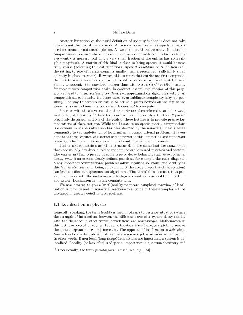
Fig. 1. Left: Localized eigenfunction. Right: Delocalized eigenfunction.
is given (up to a normalization factor) by Ψ0pxq “ sin`
2πLx˘
, which is delocalized(see Fig. 1, right).
Consider now an extended system consisting of a large number of atoms, as-sumed to be in the ground state. Suppose the system is perturbed at one pointspace, for example by slightly changing the value of the potential V near somepoint x. If the system is an insulator, then the effect of the perturbation will onlybe felt locally: it will not be felt outside of a small region. This “absence of dif-fusion” is also known as localization. W. Kohn [124, 169] called this behavior the“nearsightedness” of electronic matter. In insulators, and also in semi-conductorsand in metallic systems under suitable conditions (such as room temperature), theelectrons tend to stay put.
Localization is a phenomenon of major importance in quantum chemistry andin solid state physics. We will return on this in section 4.2, when we discuss applica-tions to the electronic structure problem. Another important example is Andersonlocalization, which refers to the localization in systems described by Hamiltoniansof the form H “ T `γV where V is a random potential and γ ą 0 a parameter thatcontrols the “disorder strength” in the system [4]. Loosely speaking, once γ exceedsa certain threshold γ0 the eigenfunctions of H abruptly undergo a transition fromextended to localized with very high probability. Anderson localization is beyondthe scope of the techniques discussed in these lectures. The interested reader isreferred to [185] for a survey.
Locality (or lack thereof) is also of central importance in quantum informationtheory and quantum computing, in connection with the notion of entanglement ofstates [77].
1.2 Localization in numerical mathematics
In contrast to the situation in physics, the recognition of localization as an im-portant property in numerical mathematics is relatively recent. It began to slowlyemerge in the late 1970s and early 1980s as a results of various trends in numericalanalysis, particularly in approximation theory (convergence properties of splines)and in numerical linear algebra. Researchers in these areas were the first to investi-gate the decay properties of inverses and eigenvectors of certain classes of banded

Localization in Matrix Computations: Theory and Applications 5
matrices; see [68, 69] and [60]. By the late 1990s, the decay behavior of the en-tries of fairly general functions of banded matrices had been analyzed [22, 117],and numerous papers on the subject have appeared since then. Figures 2-4 provideexamples of localization for different matrix functions.
From a rather different direction, Banach algebras of infinite matrices with off-diagonal decay arising in computational harmonic analysis and other problems ofa numerical nature were being investigated in the 1990s by Jaffard in France [119]and by Baskakov and others [12, 13, 34] in the former Soviet Union. In particular,much effort has been devoted to the study of classes of inverse-closed algebras ofinfinite matrices with off-diagonal decay.4 This is now a well-developed area ofmathematics; see, e.g., [97, 98, 189] as well as [141, 172]. We will return on thistopic in section 3.8.
020
4060
80100
0
20
40
60
80
1000
2
4
6
8
10
12
14
16
18
Fig. 2. Plot of |reAsij | for A tridiagonal (discrete 1D Laplacian).
Locality in numerical linear algebra is related to, but should not be confusedwith, sparsity. A matrix can be localized even if it is a full matrix, although it willbe close to a sparse matrix (in some norm).
Perhaps less obviously, a (discrete) system could well be described by a highlysparse matrix but be strongly delocalized. This happens when all the different partscomprising the system are “close together” in some sense. Network science providesstriking examples of this: small diameter graphs, and particularly small-world net-works, such as Facebook, and other online social networks, are highly sparse butdelocalized, in the sense that there is no clear distinction between “short-range”and “long-range” interactions between the components of the system. Even if, on
4 Let A Ď B be two algebras with common identity. Then A is said to be inverse-closed in B if A´1
P A for all A P A that are invertible in B [97].

6 Michele Benzi
020
4060
80100
0
20
40
60
80
1000
0.2
0.4
0.6
0.8
1
Fig. 3. Plot of |rA12sij | for matrix nos4 from the University of Florida Sparse
Matrix Collection [65] (scaled and reordered with reverse Cuthill–McKee).
020
4060
80100
020
4060
80100
0
5
10
15
Fig. 4. Plot of |rlogpAqsij | for matrix bcsstk03 from the University of FloridaSparse Matrix Collection [65] (scaled and reordered with reverse Cuthill–McKee).

Localization in Matrix Computations: Theory and Applications 7
average, each component of such a system is directly connected to only a few othercomponents, the system is strongly delocalized, since every node is only a few stepsaway from every other node. Hence, a “disturbance” at one node propagates quicklyto the entire system. Every short range interaction is also long-range: locality is al-most absent in such systems. We shall retrun to this topic in section 4.3.
Intuitively speaking, localization makes sense (for a system ofN parts embeddedin some n-dimensional space) when it is possible to let the system size N grow toinfinity while keeping the density (number of parts per unit volume) constant. Thissituation is sometimes referred to as the thermodynamic limit (or bulk limit in solidstate physics). We will provide a more formal discussion of this in a later section ofthe paper using notions from graph theory.
It is interesting to observe that both localization and delocalization can be ad-vantageous from a computational perspective. Computing approximations to vec-tors or matrices that are strongly localized can be very efficient in terms of bothstorage and arithmetic complexity, but computations with systems that are bothsparse and delocalized (in the sense just discussed) can also be very efficient, sinceinformation propagates very quickly in such systems. As a result, iterative methodsbased on matrix vector products for solving linear systems, computing eigenvaluesand evaluating matrix functions tend to converge very quickly for sparse problemscorresponding to small-diameter graphs; see, e.g., [5].
2 Notation and background in linear algebra and graphtheory
In this chapter we provide the necessary background in linear algebra and graphtheory. Excellent general references for linear algebra and matrix analysis are thetwo volumes by Horn and Johnson [113, 114]. For a thorough treatment of matrixfunctions, see the monograph by Higham [109]. A good general introduction tograph theory is Diestel [72].
We will be dealing primarily with matrices and vectors with entries in R or C.The pi, jq entry of matrix A will be denoted either by aij or by rAsij . Throughoutthis chapter, I will denote the identity matrix (or operator); the dimension shouldbe clear from the context.
Recall that a matrix A P Cnˆn is Hermitian if A˚ “ A, skew-Hermitian ifA˚ “ ´A, unitary if A˚ “ A´1, symmetric if AT “ A, skew-symmetric if AT “ ´A,and orthogonal if AT “ A´1. A matrix A is diagonalizable if it is similar to adiagonal matrix: there exist a diagonal matrix D and a nonsingular matrix X suchthat A “ XDX´1. The diagonal entries of D are the eigenvalues of A, denotedby λi, and they constitute the spectrum of A, denoted by σpAq. The columns ofX are the corresponding eigenvectors. A matrix A is unitarily diagonalizable ifA “ UDU˚ with D diagonal and U unitary. The spectral theorem states that anecessary and sufficient condition for a matrix A to be unitarily diagonalizable isthat A is normal: AA˚ “ A˚A. Hermitian, skew-Hermitian and unitary matricesare examples of normal matrices.
Any matrix A P Cnˆn can be reduced to Jordan form. Let λ1, . . . , λs P C bethe distinct eigenvalues of A. Then there exists a nonsingular Z P Cnˆn such thatZ´1AZ “ J “ diagpJ1, J2, . . . , Jsq, where each diagonal block J1, J2, . . . , Js is block

8 Michele Benzi
diagonal and has the form Ji “ diagpJp1qi , J
p2qi , . . . , J
pgiqi q, where gi is the geometric
multiplicity of the λi,
Jpjqi “
»
—
—
—
—
—
–
λi 1 0 . . . 00 λi 1 . . . 0...
.... . .
. . ....
0 0 . . . λi 10 0 . . . 0 λi
fi
ffi
ffi
ffi
ffi
ffi
fl
P Cνpjqi ˆν
pjqi ,
andřsi“1
řgij“1 ν
pjqi “ n. The Jordan matrix J is unique up to the ordering of
the blocks, but Z is not. The order ni of the largest Jordan block in which theeigenvalue λi appears is called the index of λi. If the blocks Ji are ordered fromlargest to smallest, then indexpλiq “ ν
p1qi . A matrix A is diagonalizable if and only
if all the Jordan blocks in J are 1ˆ 1.From the Jordan decomposition of a matrix A P Cnˆn we obtain the following
“coordinate-free” form of the Jordan decomposition of A:
A “sÿ
i“1
rλiGi `Nis (1)
where λ1, . . . , λs are the distinct eigenvalues of A, Gi is the projector onto thegeneralized eigenspace KerppA´λiIq
niq along RanppA´λiIqniq with ni “ indexpλiq,
and Ni “ pA ´ λiIqGi “ GipA ´ λiIq is nilpotent of index ni. The Gi’s are theFrobenius covariants of A.
If A is diagonalizable (A “ XDX´1) then Ni “ 0 and the expression above canbe written
A “nÿ
i“1
λi xiy˚i
where λ1, . . . , λn are not necessarily distinct eigenvalues, and xi, yi are right andleft eigenvectors of A corresponding to λi. Hence, A is a weighted sum of at mostn rank-one matrices (oblique projectors).
If A is normal then the spectral theorem yields
A “nÿ
i“1
λiuiu˚i
where ui is eigenvector corresponding to λi. Hence, A is a weighted sum of at mostn rank-one orthogonal projectors.
From these expressions one readily obtains for any matrix A P Cnˆn that
Tr pAq :“nÿ
i“1
aii “nÿ
i“1
λi
and, more generally,
Tr pAkq “nÿ
i“1
λki , @k “ 1, 2, . . .
Next, we recall the singular value decomposition (SVD) of a matrix. For anyA P Cmˆn there exist unitary matrices U P Cmˆm and V P Cnˆn and a “diagonal”matrix Σ P Rmˆn such that

Localization in Matrix Computations: Theory and Applications 9
U˚AV “ Σ “ diag pσ1, . . . , σpq
where p “ mintm,nu. The σi are the singular values of A and satisfy (for A ‰ 0)
σ1 ě σ2 ě ¨ ¨ ¨ ě σr ą σr`1 “ ¨ ¨ ¨ “ σp “ 0 ,
where r “ rankpAq. The matrix Σ is uniquely determined by A, but U and Vare not. The columns ui and vi of U and V are left and right singular vectorsof A corresponding to the singular value σi. From AA˚ “ UΣΣTU˚ and A˚A “V ΣTΣV ˚ we deduce that the singular values of A are the (positive) square rootsof the eigenvalues of the matrices AA˚ and A˚A; the left singular vectors of A areeigenvectors of AA˚, and the right ones are eigenvectors of A˚A. Moreover,
A “rÿ
i“1
σi uiv˚i ,
showing that any matrix A of rank r is the sum of exactly r rank-one matrices.The notion of a norm on a vector space (over R or C) is well known. A matrix
norm on the matrix spaces Rnˆnor Cnˆn is just a vector norm ¨ which satisfiesthe additional requirement of being submultiplicative:
AB ď AB, @A,B .
Important examples of matrix norms include the Frobenius norm
AF :“
g
f
f
e
nÿ
i“1
nÿ
j“1
|aij |2
as well as the norms
A1 “ max1ďjďn
nÿ
i“1
|aij |, A8 “ A˚1 “ max
1ďiďn
nÿ
j“1
|aij |
and the spectral norm A2 “ σ1. Note that AF “a
řni“1 σ
2i and therefore
A2 ď AF for all A. The inequality
A2 ďa
A1A8 (2)
is often useful; note that for A “ A˚ it implies that A2 ď A1 “ A8.The spectral radius %pAq :“ maxt|λ| : λ P σpAqu satisfies %pAq ď A for all A
and all matrix norms. For a normal matrix, %pAq “ A2. But if A is nonnormal,A2 ´ %pAq can be arbitrarily large. Also note that if A is diagonalizable withA “ XDX´1, then
A2 “ XDX´12 ď X2X
´12D2 “ κ2pXq%pAq ,
where κ2pXq “ X2X´12 is defined as the infimum of the spectral condition
numbers of X taken over the set of all matrices X which diagonalize A.Clearly, the spectrum σpAq is entirely contained in the closed disk in the complex
plane centered at the origin with radius %pAq. Much effort has been devoted tofinding better “inclusion regions,” i.e., subsets of C containing all the eigenvaluesof a given matrix. We review some of these next.

10 Michele Benzi
Let A P Cnˆn. For all i “ 1, . . . , n, let
ri :“ÿ
j‰i
|aij |, Di “ Dipaii, riq :“ tz P C : |z ´ aii| ď riu .
The set Di is called the ith Gersgorin disk of A. Gersgorin’s Theorem (1931) statesthat σpAq Ă Yni“1Di. Moreover, each connected component of Yni“1Di consistingof p Gersgorin disks contains exactly p eigenvalues of A, counted with their multi-plicities. Of course, the same result holds replacing the off-diagonal row-sums withoff-diagonal column-sums. The spectrum is then contained in the intersection ofthe two resulting regions.
Also of great importance is the field of values (or numerical range) of A P Cnˆn,defined as the set
WpAq :“ tz “ xAx,xy : x˚x “ 1u . (3)
This set is a compact subset of C containing the eigenvalues of A; it is also convex.This last statement is known as the Hausdorff–Toeplitz Theorem, and is highlynontrivial. If A is normal, the field of values is the convex hull of the eigenvalues;the converse is true if n ď 4, but not in general. The eigenvalues and the field ofvalues of a random 10ˆ 10 matrix are shown in Fig. 5.
−1 0 1 2 3 4 5 6−1.5
−1
−0.5
0
0.5
1
1.5
Fig. 5. Eigenvalues and field of values of a random 10ˆ 10 matrix.
For a matrix A P Cnˆn, let
H1 “1
2pA`A˚q, H2 “
1
2ipA´A˚q. (4)
Note that H1, H2 are both Hermitian. Let a “ minλpH1q, b “ maxλpH1q, c “minλpH2q, and d “ maxλpH2q. Then for every eigenvalue λpAq of A we have that
a ď <pλpAqq ď b, c ď =pλpAqq ď d.
This is sometimes referred to as the Bendixson–Hirsch Theorem; see, e.g., [14,page 224]. Moreover, the field of values of A is entirely contained in the rectanglera, bsˆrc, ds in the complex plane [114, page 9]. Note that if A P Rnˆn, then c “ ´d.

Localization in Matrix Computations: Theory and Applications 11
The definition of field of values (3) also applies to bounded linear operators ona Hilbert space H ; however, WpAq may not be closed if dim pH q “ 8.
For a matrix A P Cnˆn and a scalar polynomial
ppλq “ c0 ` c1λ` c2λ2` ¨ ¨ ¨ ` ckλ
k,
defineppAq “ c0I ` c1A` c2A
2` ¨ ¨ ¨ ` ckA
k .
Let A “ ZJZ´1 where J is the Jordan form of A. Then ppAq “ ZppJqZ´1.Hence, the eigenvalues of ppAq are given by ppλiq, for i “ 1, . . . , n. In particular,if A is diagonalizable with A “ XDX´1 then ppAq “ XppDqX´1. Hence, A andppAq have the same eigenvectors.
The Cayley–Hamilton Theorem states that for any matrix A P Cnˆn it holdsthat pApAq “ 0, where pApλq :“ det pA ´ λIq is the characteristic polynomial ofA. Perhaps an even more important polynomial is the minimum polynomial of A,which is defined as the monic polynomial qApλq of least degree such that qApAq “ 0.Note that qA|pA, hence degpqAq ď degppAq “ n. It easily follows from this that forany nonsingular A P Cnˆn, the inverse A´1 can be expressed as a polynomial in Aof degree at most n´ 1:
A´1“ c0I ` c1A` c2A
2` ¨ ¨ ¨ ` ckA
k, k ď n´ 1.
Note, however, that the coefficients ci depend on A. It also follows that powersAp with p ě n can be expressed as linear combinations of powers Ak with 0 ď k ďn´ 1. The same result holds more generally for matrix functions fpAq that can berepresented as power series in A (see below).
Indeed, let λ1, . . . , λs be the distinct eigenvalues of A P Cnˆn and let ni be theindex of λi. If f is a given function, we define the matrix function
fpAq :“ rpAq,
where r is the unique Lagrange–Hermite interpolating polynomial of degree ăsř
i“1
ni
satisfyingrpjqpλiq “ f pjqpλiq j “ 0, . . . , ni ´ 1, i “ 1, . . . , s.
Here f pjq denotes the jth derivative of f , with f p0q ” f . Note that for the definitionto make sense we must require that the values f pjqpλiq with 0 ď j ď ni ´ 1 and1 ď i ď s exist. We say that f is defined on the spectrum of A. When all theeigenvalues are distinct, the interpolation polynomial has degree n´1. In this case,the minimum polynomial and the characteristic polynomial of A coincide.
There are several other ways to define fpAq, all equivalent to the definition justgiven [109]. One such definition is through the Jordan canonical form. Let A P Cnˆnhave Jordan form Z´1AZ “ J with J “ diagpJ1, . . . , Jsq. We define
fpAq :“ Z fpJqZ´1“ Z diagpfpJ1q, fpJ2q, . . . , fpJsqqZ
´1,
where fpJiq “ diagpfpJp1qi q, fpJ
p2qi q, . . . , fpJ
pgiqi qq and

12 Michele Benzi
fpJpjqi q “
»
—
—
—
—
—
—
–
fpλiq f1pλiq . . .
fpνpjqi´1q
pλiq
pνpjqi ´1q!
fpλiq. . .
...
. . . f 1pλiqfpλiq
fi
ffi
ffi
ffi
ffi
ffi
ffi
fl
.
An equivalent expression is the following:
fpAq “sÿ
i“1
ni´1ÿ
j“0
f pjqpλiq
j!pA´ λiIq
jGi,
where ni “ indexpλiq and Gi is the Frobenius covariant associated with λi (see(1)). The usefulness of this definition is primarily theoretical, given the difficultyof determining the Jordan structure of a matrix numerically. If A “ XDX´1 withD diagonal, then fpAq :“ XfpDqX´1
“ XdiagpfpλiqqX´1. Denoting with xi the
ithe column of X and with yi the ith column of X´1 we obtain the expression
fpAq “nÿ
i“1
fpλiqxiy˚i .
If in addition A “ UDU˚ is normal then
fpAq “nÿ
i“1
fpλiquiu˚i .
If f is analytic in a domain Ω Ď C containing the spectrum of A P Cnˆn, then
fpAq “1
2πi
ż
Γ
fpzqpzI ´Aq´1dz , (5)
where i “?´1 is the imaginary unit and Γ is any simple closed curve surrounding
the eigenvalues of A and entirely contained in Ω, oriented counterclockwise. Thisdefinition has the advantage of being easily generalized to functions of boundedoperators on Banach spaces, and it is also the basis for some of the currently mostefficient computational methods for the evaluation of matrix functions.
Another widely used definition of fpAq when f is analytic is through powerseries. Suppose f has a Taylor series expansion
fpzq “8ÿ
k“0
akpz ´ z0qk
ˆ
ak “f pkqpz0q
k!
˙
with radius of convergence R. If A P Cnˆn and each of the distinct eigenvaluesλ1, . . . , λs of A satisfies
|λi ´ z0| ă R,
then
fpAq :“8ÿ
k“0
akpA´ z0Iqk.
If A P Cnˆn and f is defined on σpAq, the following facts hold (see [109]):

Localization in Matrix Computations: Theory and Applications 13
(i) fpAqA “ AfpAq;(ii) fpAT q “ fpAqT ;(iii) fpXAX´1
q “ XfpAqX´1;(iv) σpfpAqq “ fpσpAqq;(v) pλ, xq eigenpair of A ñ pfpλq, xq eigenpair of fpAq;(vi) A is block triangular ñ F “ fpAq is block triangular with the same block
structure as A, and Fii “ fpAiiq where Aii is the ith diagonal block of A;(vii) In particular, fpdiag pA11, . . . , Appqq “ diag pfpA11q, . . . , fpAppqq;(viii) fpIm bAq “ Im b fpAq, where b is the Kronecker product;(ix) fpAb Imq “ fpAq b Im.
Another useful result is the following:
Theorem 1. ([110]) Let f be analytic on an open set Ω Ď C such that each con-nected component of Ω is closed under conjugation. Consider the correspondingmatrix function f on the set D “ tA P Cnˆn : σpAq Ď Ωu. Then the following areequivalent:
(a) fpA˚q “ fpAq˚ for all A P D.(b) fpAq “ fpAq for all A P D.(c) fpRnˆn XDq Ď Rnˆn.(d) fpRXΩq Ď R.
In particular, if fpxq P R for x P R and A is Hermitian, so is fpAq.Important examples of matrix functions are the resolvent and the matrix ex-
ponential. Let A P Cnˆn, and let z R σpAq. The resolvent of A at z is definedas
RpA; zq “ pzI ´Aq´1.
The resolvent is central to the definition of matrix functions via the contourintegral approach (5). The resolvent also plays a fundamental role in spectral theory.For example, it can be used to define the spectral projector onto the eigenspace ofa matrix or operator corresponding to an isolated eigenvalue λ0 P σpAq:
Pλ0 :“1
2πi
ż
|z´λ0|“ε
pzI ´Aq´1dz ,
where ε ą 0 is small enough so that no other eigenvalue of A falls within ε of λ0.It can be shown that P 2
λ0“ Pλ0 and that the range of Pλ0 is the one-dimensional
subspace spanned by the eigenvector associated with λ0. More generally, one candefine the spectral projector onto the invariant subspace of A corresponding toa set of selected eigenvalues by integrating RpA; zq along a countour surroundingthose eigenvalues and excluding the others. It should be noted that the spectralprojector is an orthogonal projector (P “ P˚) if and only if A is normal. If A isdiagonalizable, a spectral projector P is a simple function of A: if f is any functiontaking the value 1 at the eigenvalues of interest and 0 on the remaining ones, thenP “ fpAq.
The matrix exponential can be defined via the Maclaurin expansion
eA “ I `A`1
2!A2`
1
3!A3` ¨ ¨ ¨ “
8ÿ
k“0
1
k!Ak ,

14 Michele Benzi
which converges for arbitrary A P Cnˆn. Just as the resolvent is central to spec-tral theory, the matrix exponential is fundamental to the solution of differentialequations. For example, the solution to the inhomogeneous system
dy
dt“ Ay ` fpt,yq, yp0q “ y0, y P Cn, A P Cnˆn
is given (implicitly!) by
yptq “ etAy0 `
ż t
0
eApt´sqfps,ypsqqds.
In particular, yptq “ etAy0 when f “ 0. It is worth recalling that limtÑ8 etA “ 0if and only if A is a stable matrix: <pλq ă 0 for all λ P σpAq.
When fpt,yq “ b P Cn (=const.), the solution can also be expressed as
yptq “ tψ1ptAqpb`Ay0q ` y0 ,
where
ψ1pzq “ez ´ 1
z“ 1`
z
2!`z2
3!` ¨ ¨ ¨
The matrix exponential plays an especially important role in quantum theory.Consider for instance the time-dependent Schrodinger equation:
iBΨ
Bt“ HΨ, t P R, Ψp0q “ Ψ0, (6)
where Ψ0 P L2 is a prescribed initial state with Ψ02 “ 1. Here H “ H˚ is the
Hamiltonian, or energy operator (which we assume to be time-independent). Thesolution of (6) is given explicitly by Ψptq “ e´itHΨ0, for all t P R; note that sinceitH is skew-Hermitian, the propagator Uptq “ e´itH is unitary, which guaranteesthat the solution has unit norm for all t:
Ψptq2 “ UptqΨ02 “ Ψ02 “ 1, @ t P R.
Also very important in many-body quantum mechanics is the Fermi–Dirac op-erator, defined as
fpHq :“ pI ` exppβpH ´ µIqqq´1 ,
where β “ pκBT q´1 is the inverse temperature, κB the Boltzmann constant, and
µ is the Fermi level, separating the eigenvalues of H corresponding to the first neeigenvectors from the rest, where ne is the number of particles (electrons) com-prising the system under study. This matrix function will be discussed in section4.2.
Finally, in statistical quantum mechanics the state of a system is completelydescribed (statistically) by the density operator:
ρ :“e´βH
Z, where Z “ Tr pe´βHq.
The quantity Z “ Zpβq is known as the partition function of the system.Trigonometric functions and square roots of matrices are also important in
applications to differential equations. For example, the solution to the second-ordersystem

Localization in Matrix Computations: Theory and Applications 15
d2y
dt2`Ay “ 0, yp0q “ y0, y1p0q “ y10
(where A is SPD) can be expressed as
yptq “ cosp?Atqy0 ` p
?Aq´1 sinp
?Atqy10 .
Apart from the contour integration formula, the matrix exponential and theresolvent are also related through the Laplace transform: there exists an ω P R suchthat z R σpAq for <pzq ą ω and
pzI ´Aq´1“
ż 8
0
e´ztetAdt “
ż 8
0
e´tpzI´Aqdt .
Also note that if |z| ą %pAq, the following Neumann series expansion of theresolvent is valid:
pzI ´Aq´1“ z´1
pI ` z´1A` z´2A2` ¨ ¨ ¨ q “ z´1
8ÿ
k“0
z´kAk.
Next, we recall a few definitions and notations associated with graphs. LetG “ pV, Eq be a graph with n “ |V| nodes (or vertices) and m “ |E | edges (orlinks). The elements of V will be denoted simply by 1, . . . , n. If for all i, j P V suchthat pi, jq P E then also pj, iq P E , the graph is said to be undirected. On the otherhand, if this condition does not hold, namely if there exists pi, jq P E such thatpj, iq R E , then the network is said to be directed. A directed graph is commonlyreferred to as a digraph. If pi, jq P E in a digraph, we will write i Ñ j. A graphis simple if it is unweighted, contains no loops (edges of the form pi, iq) and thereare no multiple edges with the same orientation between any two nodes. A simplegraph can be represented by means of its adjacency matrix A “ raijs P Rnˆn, where
aij “
"
1, if pi, jq P E ,0, else.
Note that A “ AT if, and only if, G is undirected. If the graph is weighted, thenaij will be equal to the weight of the corresponding edge pi, jq.
If G is undirected, the degree degpiq of node i is the number of edges incident toi in G. That is, degpiq is the number of “immediate neighbors” of i in G. Note thatin terms of the adjacency matrix, degpiq “
řnj“1 aij . A d-regular graph is a graph
where every node has the same degree d.For an undirected graph we also define the graph Laplacian as the matrix
L :“ D ´A, where D :“ diagpdegp1q,degp2q, . . . , degpnqq
and, assuming degpiq ‰ 0 for all i, the normalized Laplacian
pL :“ I ´D´12AD´12.
Both of these matrices play an important role in the structural analysis of networksand in the study of diffusion-type process on graphs, and matrix exponentials of
the form e´tL and e´tpL, where t ą 0 denotes time, are widely used in applications.
Note that L and L are both symmetric positive semidefinite matrices. Moreover,if G is a d-regular graph, then the eigenvalues of L are given by d ´ λipAq (where

16 Michele Benzi
λipAq are the eigenvalues of the adjacency matrix A of G) and L and A have thesame eigenvectors. For more general graphs, however, there is no simple relationshipbetween the spectra of L and A.
A walk of length k in G is a set of nodes ti1, i2, . . . ik, ik`1u such that for all1 ď j ď k, there is an edge between ij and ij`1 (a directed edge ij Ñ ij`1 for adigraph). A closed walk is a walk where i1 “ ik`1. A path is a walk with no repeatednodes.
There is a close connection between the walks in G and the entries of the powersof the adjacency matrix A. Indeed, let k ě 1. For any simple graph G, the followingholds:
rAksii “ number of closed walks of length k starting and ending at node i;rAksij “ number of walks of length k starting at node i and ending at node j.
Let now i and j be any two nodes in G. In many situations in network science itis desirable to have a measure of how “well connected” nodes i and j are. Estradaand Hatano [80] have proposed to quantify the strength of connection betweennodes in terms of the number of walks joining i and j, assigning more weight toshorter walks (i.e., penalizing longer ones). If walks of length k are downweightedby a factor 1
k!, this leads [80] to the following definition of communicability between
node i and node j:
Cpi, jq :“ reAsij “8ÿ
k“0
rAksijk!
, (7)
where by convention we assign the value 1 to the number of “walks of length 0.”Of course, other matrix functions can also be used to define the communicabilitybetween nodes [82], but the matrix exponential has a natural physical interpretation(see [81]).
The geodesic distance dpi, jq between two nodes i and j is the length of theshortest path connecting i and j. We let dpi, jq “ 8 if no such path exists. We notethat dp¨, ¨q is a true distance function (i.e., a metric on G) if the graph is undirected,but not in general, since only in an undirected graph the condition dpi, jq “ dpj, iqis satisfied for all i P V.
The diameter of a graph G “ pV, Eq is defined as
diampGq :“ maxi,jPV
dpi, jq .
A digraph G is strongly connected (or, in short, connected) if for every pair ofnodes i and j there is a path in G that starts at i and ends at j; i.e., diampGq ă 8.We say that G is weakly connected if it is connected as an undirected graph (i.e.,when the orientation of the edges is disregarded). Clearly, for an undirected graphthe two notions coincide. It can be shown that for an undirected graph the numberof connected components is equal to the dimension of KerpLq, the null space of thegraph Laplacian.
Just as we have associated matrices to graphs, graphs can also be associatedto matrices. In particular, to any matrix A P Cnˆn we can associate a digraphGpAq “ pV, Eq where V “ t1, 2, . . . , nu and E Ď V ˆ V, where pi, jq P E if and onlyif aij ‰ 0. Diagonal entries in A are usually ignored, so that there are no loops inGpAq. We also note that for structurally symmetric matrices (aij ‰ 0 ô aji ‰ 0)the associated graph GpAq with A is undirected.
Localization in Matrix Computations: Theory and Applications 17
Let |A| :“ r |aij | s, then the digraph Gp|A|2q is given by pV, Eq where E is ob-tained by including all directed edges pi, kq such that there exists j P V withpi, jq P E and pj, kq P E . (The reason for the absolute value is to disregard the effectof possible cancellations in A2.) For higher powers `, the digraph Gp|A|`q is definedsimilarly: its edge set consists of all pairs pi, kq such that there is a directed pathof length at most ` joining node i with node k in GpAq.
0 10 20 30 40 50 60 70 80 90 100
0
10
20
30
40
50
60
70
80
90
100
nz = 3010 10 20 30 40 50 60 70 80 90 100
0
10
20
30
40
50
60
70
80
90
100
nz = 1081
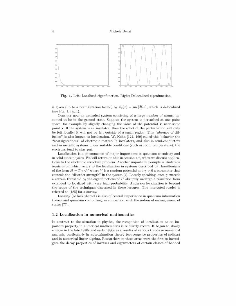
Fig. 6. Path graph. Left: nonzero pattern of Laplacian matrix L. Right: pattern offifth power of L.
0 200 400 600 800 1000 1200 1400 1600 1800 2000
0
200
400
600
800
1000
1200
1400
1600
1800
2000
nz = 9948
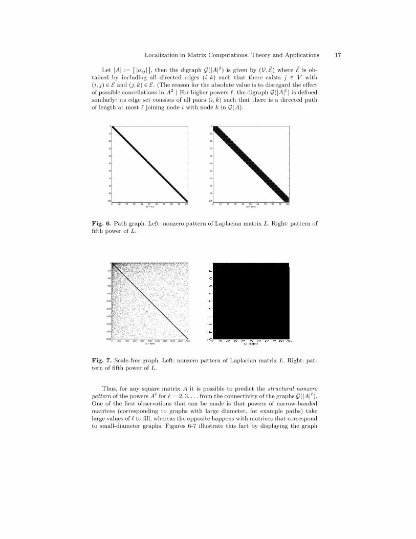
Fig. 7. Scale-free graph. Left: nonzero pattern of Laplacian matrix L. Right: pat-tern of fifth power of L.
Thus, for any square matrix A it is possible to predict the structural nonzeropattern of the powers A` for ` “ 2, 3, . . . from the connectivity of the graphs Gp|A|`q.One of the first observations that can be made is that powers of narrow-bandedmatrices (corresponding to graphs with large diameter, for example paths) takelarge values of ` to fill, whereas the opposite happens with matrices that correspondto small-diameter graphs. Figures 6-7 illustrate this fact by displaying the graph

18 Michele Benzi
Laplacian L and the fifth power of L for two highly sparse undirected graphs, apath graph with n “ 100 nodes and a scale-free graph on n “ 2000 nodes builtaccording to preferential attachment scheme (see, e.g., [79]). Graphs of this type areexamples of small-world graphs, in particular they can be expected to have smalldiameter. It can be seen that in the case of the scale-free graph the fifth power ofthe Laplacian, L5, is almost completely full (the number of nonzeros is 3, 601, 332out of a possible 4, 000, 000), implying that in this graph most pairs of nodes areless than five degrees of separation away from one another.
The transitive closure of G is the graph G “ pV, Eq where pi, jq P E if and onlyif there is a directed path from i to j in GpAq. A matrix A P Cnˆn is reducible ifthere exists a permutation matrix P such that
PTAP “
„
A11 A12
0 A22
with A11 and A22 square submatrices. If no such P exists, A is said to be irreducible.Denote by Kn the complete graph on n nodes, i.e., the graph where every edge pi, jqis present (with i ‰ j). The following statements are equivalent:
(i) the matrix A is irreducible;(ii) the digraph GpAq is strongly connected;(iii) the transitive closure GpAq of GpAq is Kn.
Note that (iii) and the Cayley–Hamilton Theorem imply that the powers pI `|A|qk are completely full for k ě n´ 1. This has important implications for matrixfunctions, since it implies that for an irreducible matrix A a matrix function of theform
fpAq “8ÿ
k“0
akpA´ z0Iqk
is completely full, if no cancellation occurs and ak ‰ 0 for sufficiently many k. Thisis precisely formulated in the following result.
Theorem 2. ([24]) Let f be an analytic function of the form
fpzq “8ÿ
k“0
akpz ´ z0qk
ˆ
ak “f pkqpz0q
k!
˙
,
where z0 P C and the power series expansion has radius of convergence R ą 0. LetA have an irreducible sparsity pattern and let l (1 ď l ď n ´ 1) be the diameterof GpAq. Assume further that there exists k ě l such that f pkqpz0q ‰ 0. Then itis possible to assign values to the nonzero entries of A in such a way that fpAq isdefined and rfpAqsij ‰ 0 for all i ‰ j.
This result applies, in particular, to banded A and to such functions as theinverse (resolvent) and the matrix exponential.
3 Localization in matrix functions
We have just seen that if A is irreducible and f is a “generic” analytic functiondefined on the spectrum of A then we should expect fpAq to be completely full

Localization in Matrix Computations: Theory and Applications 19
(barring fortuitous cancellation). For A large, this seems to make the explicit com-putation of fpAq impossible, and this is certainly the case if all entries of fpAq needto be accurately approximated.
As we have already mentioned in the Introduction, however, numerical exper-iments show that when A is a banded matrix and fpzq is a smooth function forwhich fpAq is defined, the entries of fpAq often decay rapidly as one moves awayfrom the diagonal. The same property is often (but not always!) satisfied by moregeneral sparse matrices: in this case the decay is away from the support (nonzeropattern) of A. In other words, nonnegligible entries of fpAq tend to be concentratednear the positions pi, jq for which aij ‰ 0.
This observation opens up the possibility of approximating functions of sparsematrices, by neglecting “sufficiently small” matrix elements in fpAq. Depending onthe rate of decay and on the accuracy requirements, it may be possible to developapproximation algorithms that exhibit optimal computational complexity, i.e., Opnq(or linear scaling) methods.
In this section we review our current knowledge on localization in functions oflarge and sparse matrices. In particular, we consider the following questions:
1. Under which conditions can we expect decay in fpAq?2. Can we obtain sharp bounds on the entries of fpAq?3. Can we characterize the rate of decay in fpAq in terms of
– the bandwidth/sparsity of A?– the spectral properties of A?– the location of singularities of fpzq in relation to the spectrum of A?
4. What if fpzq is an entire5 function?5. When is the rate of decay independent of the matrix size n?
The last point is especially crucial if we want to develop Opnq algorithms forapproximating functions of sparse matrices.
3.1 Matrices with decay
A matrix A P Cnˆn is said to have the off-diagonal decay property if its entries rAsijsatisfy a bound of the form
|rAsij | ď Kφp|i´ j|q, @ i, j, (8)
where K ą 0 is a constant and φ is a function defined and positive for x ě 0 andsuch that φpxq Ñ 0 as x Ñ 8. Important examples of decay include exponentialdecay, corresponding to φpxq “ e´αx for some α ą 0, and algebraic (or power-law)decay, corresponding to φpxq “ p1` |i´ j|pq´1 for some p ě 1.
As it stands, however, this definition is meaningless, since for any fixed matrixA P Cnˆn the bound can always be achieved with an arbitrary choice of φ justby taking K sufficiently large. To give a meaningful definition we need to considereither infinite matrices (for example, bounded linear operators on some sequencespace `p), or sequences of matrices of increasing dimension. The latter situationbeing the more familiar one in numerical analysis, we give the following definition.
5 Recall that an entire function is a function of a complex variable that is analyticeverywhere on the complex plane.

20 Michele Benzi
Definition 1. Let tAnu be a sequence of n ˆ n matrices with entries in C, wherenÑ 8. We say that the matrix sequence tAnu has the off-diagonal decay propertyif
|rAnsij | ď Kφp|i´ j|q, @ i, j “ 1, . . . , n, (9)
where the constant K ą 0 and the function φpxq, defined for x ě 0 and such thatφpxq Ñ 0 as xÑ8, do not depend on n.
Note that if A is an infinite matrix that satisfies (8) then its finite nˆn sections(leading principal submatrices, see [141]) An form a matrix sequence that satisfiesDef. 1. The definition can also be extended to block matrices in a natural way.
When dealing with non-Hermitian matrices, it is sometimes required to allowfor different decay rates on either side of the main diagonal. For instance, one couldhave exponential decay on either side but with different rates:
|rAnsij | ď K1 e´αpi´jq for i ą j ,
and|rAnsij | ď K2 e´βpj´iq for j ą i .
Here K1,K2 and α, β are all positive constants. It is also possible to have matriceswhere decay is present on only one side of the main diagonal (see [24, Theorem3.5]). For simplicity, in the rest of the paper we will primarily focus on the casewhere the decay bound has the same form for i ą j and for j ą i. However, mostof the results can be extended easily to the more general case.
Also, in multidimensional problems it is important to be able to describe decaybehavior not just away from the main diagonal but with a more complicated pattern.To this end, we can use any distance function (metric) d (with dpi, jq “ dpj, iq forsimplicity) with the property that
@ε ą 0 D c “ cpεq such that supj
ÿ
i
e´εdpi,jq ď cpεq, (10)
see [119]. Again, condition (10) is trivially satisfied for any distance function on afinite set S “ t1, 2, . . . , nu, but here we allow infinite (S “ N) or bi-infinite matrices(S “ Z). In practice, we will consider sequences of matrices of increasing size n andwe will define for each n a distance dn on the set S “ t1, 2, . . . , nu and assume thateach dn satisfies condition (10) with respect to a constant c “ cpεq independent ofn.
We will be mostly concerned with decay away from a sparsity pattern. Forbanded sparsity patterns, this is just off-diagonal decay. For more general sparsitypatterns, we assume that we are given a sequence of sparse graphs Gn “ pVn, Enqwith |Vn| “ n and |En| “ Opnq and a distance function dn satisfying (10) uniformlywith respect to n. In practice we will take dn to be the geodesic distance on Gn andwe will impose the following bounded maximum degree condition:
supntdegpiq | i P Gnu ă 8 . (11)
This condition guarantees that the distance dnpi, jq grows unboundedly as|i ´ j| does, at a rate independent of n for n Ñ 8. In particular, we have thatlimnÑ8 diampGnq “ 8. This is necessary if we want the entries of matrices withdecay to actually go to zero with the distance as nÑ8.

Localization in Matrix Computations: Theory and Applications 21
Let us now consider a sequence of nˆn matrices An with associated graphs Gnand graph distances dnpi, jq. We will say that An has the exponential decay propertyrelative to the graph Gn if there are constants K ą 0 and α ą 0 independent of nsuch that
|rAnsij | ď K e´αdnpi,jq, for all i, j “ 1, . . . , n, @n P N. (12)
The following two results says that matrices with decay can be “uniformly wellapproximated” by sparse matrices.
Theorem 3. ([20]) Let tAnu be a sequence of n ˆ n matrices satisfying the expo-nential decay property (12) relative to a sequence of graphs tGnu having uniformlybounded maximal degree. Then, for any given 0 ă δ ă K, each An contains at mostOpnq entries greater than δ in magnitude.
Theorem 4. ([24]) Let the matrix sequence tAnu satisfy the assumptions of Theo-rem 3. Then, for all ε ą 0 and for all n there exists an nˆn matrix An containingonly Opnq nonzeros such that
An ´ An1 ă ε. (13)
For example, suppose the each matrix in the sequence tAnu satisfies the fol-lowing exponential decay property: there exist K, α ą 0 independent of n suchthat
|rAnsij | ď Ke´α|i´j|, @ i, j “ 1, . . . , n, @n P N.Then, for any ε ą 0, there is a sequence of p-banded matrices An, with p indepen-dent of n, such that An ´ An1 ă ε. The matrices An can be defined as follows:
rAnsij “
#
rAnsij if |i´ j| ď p;
0 otherwise,
where p satisfies
p ě
Z
1
αlog
ˆ
2K
1´ e´αε´1
˙^
. (14)
Note that An is the orthogonal projection of An, with respect to the innerproduct associated with the Frobenius norm, onto the linear subspace of Cnˆn ofp-banded matrices.
Similar approximation results hold for other matrix norms. For instance, usingthe inequality (2) one can easily satisfy error bounds in the matrix 2-norm.
Remark 1. As mentioned in [20], similar results also hold for other types of decay;for instance, it suffices to have algebraic decay of the form
|rAnsij | ď K p|i´ j|p ` 1q´1@ i, j, @n P N,
with p ą 1. However, this type of decay is often too slow to be useful in practice,in the sense that any sparse approximation An to An would have to have Opnqnonzeros with a huge prefactor in order to satisfy (13) for even moderately smallvalues of ε.

22 Michele Benzi
3.2 Decay bounds for the inverse
It has long been known that the entries in the inverse of banded matrices arebounded in a decaying manner away from the main diagonal, with the decay beingfaster for more diagonally dominant matrices [68]. In 1984, Demko, Moss and Smith[69] proved that the entries of A´1, where A is Hermitian positive definite and m-banded (rAsij “ 0 if |i ´ j| ą m), satisfy the following exponential off-diagonaldecay bound:
|rA´1sij | ď K ρ|i´j|, @ i, j. (15)
Here we have set
K “ maxta´1,K0u, K0 “ p1`?κq2b, κ “
b
a, (16)
where ra, bs is the smallest interval containing the spectrum σpAq of A, and
ρ “ q1m, q “ qpκq “
?κ´ 1
?κ` 1
. (17)
Hence, the decay bound deteriorates as the relative distance between the spectrumof A and the singularity at zero of the function fpxq “ x´1 tends to zero (i.e., asκÑ 8) and/or if the bandwidth m increases. The bound is sharp (being attainedfor certain tridiagonal Toeplitz matrices). The result holds for n ˆ n matrices aswell as for bounded, infinite matrices acting on the Hilbert space `2. We also notethat the bound (15) can be rewritten as
|rA´1sij | ď Ke´α|i´j|, @ i, j, (18)
where we have set α “ ´ logpρq.It should be emphasized that (15) is a just a bound: the off-diagonal decay in
A´1 is in general not monotonic. Furthermore the bound, although sharp, may bepessimistic in practice.
The result of Demko et al. implies that if we are given a sequence of n ˆ nmatrices tAnu of increasing size, all Hermitian, positive definite, m-banded (withm ă n0) and such that
σpAnq Ă ra, bs @n ě n0, (19)
then the bound (15) holds for all matrices of the sequence; in other words, if thespectra σpAnq are bounded away from zero and infinity uniformly in n, the entriesof A´1
n are uniformly bounded in an exponentially decaying manner (i.e., the decayrates are independent of n). Note that it is not necessary that all matrices haveexactly the same bandwidth m, as long as they are banded with bandwidth lessthan or equal to a constant m.
The requirement that the matrices An have uniformly bounded condition num-ber as n Ñ 8 is restrictive. For example, it does not apply to banded or sparsematrices that arise from the discretization of differential operators, or in fact of anyunbounded operator. Consider for example the sequence of tridiagonal matrices
An “ pn` 1q2 tridiagp´1 , 2 ,´1q
which arise from the three-point finite difference approximation with mesh spacing
h “ 1n`1
of the operator T “ ´ d2
dx2with zero Dirichlet conditions at x “ 0 and x “

Localization in Matrix Computations: Theory and Applications 23
1. For nÑ8 the condition number of An grows like Opn2q, and although the entries
of each inverse A´1n satisfy a bound of the type (15), the spectral condition number
κ2pAnq is unbounded and therefore the bound deteriorates since K “ Kpnq Ñ 1π2
and ρ “ ρpnq Ñ 1 as nÑ8. Moreover, in this particular example the actual decayin A´1
n (and not just the bound) slows down as hÑ 0. This is to be expected sinceA´1n is trying to approximate the Green’s function of T , which does not fall off
exponentially.Nevertheless, this result is important for several reasons. First of all, families of
banded or sparse matrices (parameterized by the dimension n) exhibiting boundedcondition numbers do occur in applications. For example, under mild conditions,mass matrices in finite element analysis and overlap matrices in quantum chem-istry satisfy such conditions (these matrices represent the identity operator withrespect to some non-orthogonal basis set tφiu
ni“1, where the φi are strongly lo-
calized in space). Second, the result is important because it suggests a possiblesufficient condition for the existence of a uniform exponential decay bound in moregeneral situations: the relative distance of the spectra σpAnq from the singularitiesof the function must remain strictly positive as nÑ8. Third, it turns out that themethod of proof used in [69] works with minor changes also for more general func-tions and matrix classes, as we shall see. The proof of (15) is based on a classicalresult of Chebyshev on the uniform approximation error
min maxaďxďb
|pkpxq ´ x´1|
(where the minimum is taken over all polynomials pk of degree ď k), according towhich the error decays exponentially in the degree k as k Ñ8. Combined with thespectral theorem (which allows to go from scalar functions to matrix functions, withthe ¨ 2 matrix norm replacing the ¨ 8 norm), this result gives the exponentialdecay bound for rA´1
sij . A crucial ingredient of the proof is the fact that if A ism-banded, then Ak is km-banded, for all k “ 0, 1, 2, . . ..
The paper of Demko et al. also contains some extensions to the case of non-Hermitian matrices and to matrices with a general sparsity pattern. Invertible,non-Hermitian matrices are dealt with by observing that for any A P Cnˆn one canwrite
A´1“ A˚pAA˚q´1 (20)
and that if A is banded, then the Hermitian positive definite matrix AA˚ is alsobanded (albeit with a larger bandwidth). It is not difficult to see that the productof two matrices, one of which is banded and the other has entries that satisfy anexponential decay bound, is also a matrix with entries that satisfy an exponentialdecay bound.
For a general sparse matrix, the authors of [69] observe that the entries of A´1
are bounded in an exponentially decaying manner away from the support (nonzeropattern) of A. This fact can be expressed in the form
|rA´1sij | ď Ke´αdpi,jq, @ i, j, (21)
where dpi, jq is the geodesic distance between nodes i and j in the undirected graphGpAq associated with A.
Results similar to those in [69] where independently obtained by Jaffard [119],motivated by problems concerning wavelet expansions. In this paper Jaffard proves

24 Michele Benzi
exponential decay bounds for the entries of A´1 and mentions that similar boundscan be obtained for other matrix functions, such as A´12 for A positive definite.Moreover, the bounds are formulated for (in general, infinite) matrices the entriesof which are indexed by the elements of a suitable metric space, allowing the authorto obtain decay results for the inverses of matrices with arbitrary nonzero patternand even of dense matrices with decaying entries (we will return to this topic insection 3.8).
The exponential decay bound (15) together with Theorem 4 implies the follow-ing (asymptotic) uniform approximation result.
Theorem 5. Let tAnu be a sequence of n ˆ n matrices, all Hermitian positivedefinite and m-banded. Assume that there exists an interval ra, bs, 0 ă a ă b ă 8,such that σpAnq Ă ra, bs, for all n. Then, for all ε ą 0 and for all n there exist aninteger p “ ppε,m, a, bq (independent of n) and a matrix Bn “ B˚n with bandwidthp such that A´1
n ´Bn2 ă ε.
The smallest value of the bandwidth p needed to satisfy the prescribed accuracycan be easily computed via (14). As an example, for tridiagonal matrices An (m “
1), K “ 10, α “ 0.6 (which corresponds to ρ « 0.5488) we find A´1n ´Bn2 ă 10´6
for all p ě 29, regardless of n. In practice, of course, this result is of interest onlyfor n ą p (in fact, for n " p).
We note that a similar result holds for sparse matrix sequences tAnu corre-sponding to a sequence of graphs Gn “ pVn, Enq satisfying the assumption (11) ofbounded maximum degree. In this case the matrices Bn will be sparse rather thanbanded, with a maximum number p of nonzeros per row which does not depend onn; in other words, the graph sequence GpBnq associated with the matrix sequencetBnu will also satisfy a condition like (11).
The proof of the decay bound (15) shows that for any prescribed value of ε ą0, each inverse matrix A´1
n can be approximated within ε (in the 2-norm) by apolynomial pkpAnq of degree k in An, with k independent of n. To this end, itsuffices to take the (unique) polynomial of best approximation of degree k of thefunction fpxq “ x´1, with k large enough that the error satisfies
maxaďxďb
|pkpxq ´ x´1| ă ε.
In this very special case an exact, closed form expression for the approximationerror is known ; see [150, pages 33–34]. This expression yields an upper bound forthe error pkpAnq´A
´1n 2, uniform in n. Provided that the assumptions of Theorem
5 are satisfied, the degree k of this polynomial does not depend on n, but only onε. This shows that it is in principle possible to approximate A´1
n using only Opnqarithmetic operations and storage.
Remark 2. The polynomial of best approximation to the function fpxq “ x´1 foundby Chebyshev does not yield a practically useful expression for the explicit ap-proximation of A´1. However, observing that for any invertible matrix A and anypolynomial p
A´1´ ppAq2
A´12ď I ´ ppAqA2,
we can obtain an upper bound on the relative approximation error by finding thepolynomial of smallest degree k for which

Localization in Matrix Computations: Theory and Applications 25
maxaďxďb
|1´ pkpxqx| “ min . (22)
Problem (22) admits an explicit solution in terms of shifted and scaled Chebyshevpolynomials; see, e.g., [176, page 381]. Other procedures for approximating theinverse will be briefly mentioned in section 4.1.
A number of improvements, extensions, and refinements of the basic decayresults by Demko et al. have been obtained by various authors, largely motivatedby applications in numerical analysis, mathematical physics and signal processing,and the topic continues to be actively researched. Decay bounds for the inverses ofM -matrices that are near to Toeplitz matrices (a structure that arises frequentlyin the numerical solution of partial differential equations) can be found in Eijkhoutand Polman [76]. Freund [85] obtains an exponential decay bound for the entries ofthe inverse of a banded matrix A of the form
A “ c I ` d T, T “ T˚, c, d P C.
Exponential decay bounds for resolvents ad eigenvectors of infinite banded matriceswere obtained by Smith [184]. Decay bounds for the inverses of nonsymmetric bandmatrices can be found in a paper by Nabben [156]. The paper by Meurant [153]provides an extensive treatment of the tridiagonal and block tridiagonal cases. In-verses of triangular Toeplitz matrices arising from the solution of integral equationsalso exhibit interesting decay properties; see [84].
A recent development is the derivation of bounds that accurately capture theoscillatory decay behavior observed in the inverses of sparse matrices arising fromthe discretization of multidimensional partial differential equations. In [48], Canutoet al. obtain bounds for the inverse of matrices in Kronecker sum form, i.e., matricesof the type
A “ T1 ‘ T2 :“ T1 b I ` I b T2, (23)
with T1 and T2 banded (for example, tridiagonal). For instance, the 5-point finitedifference scheme for the discretization of the Laplacian on a rectangle producesmatrices of this form. Generalization to higher-dimensional cases (where A is theKronecker sum of three or more banded matrices) is also possible.
3.3 Decay bounds for the matrix exponential
As we have seen in the Introduction, the entries in the exponential of bandedmatrices can exhibit rapid off-diagonal decay (see Fig. 2). As it turns out, theactual decay rate is faster than exponential (the term superexponential is oftenused), a phenomenon common to all entire functions of a matrix. More precisely,we have the following definition.
Definition 2. A matrix A has the superexponential off-diagonal decay property iffor any α ą 0 there exists a K ą 0 such that
|rAsij | ď Ke´α|i´j| @ i, j.
As usual, in this definition A is either infinite or a member of a sequence ofmatrices of increasing order, in which case K and α do not depend on the order.

26 Michele Benzi
The definition can be readily extended to decay with respect to a general nonzeropattern, in which case |i ´ j| must be replaced by the geodesic distance on thecorresponding graph.
A superexponential decay bound on the entries of the exponential of a tridiag-onal matrix has been obtained by Iserles [117]. The bound takes the form
|reAsij | ď eρI|i´j|p2ρq, i, j “ 1, . . . , n (24)
where ρ “ maxi,j |rAijs| and Iνpzq is the modified Bessel function of the first kind:
Iνpzq “
ˆ
1
2z
˙ν 8ÿ
k“0
`
14z2˘k
k!Γ pν ` k ` 1q,
where ν P R and Γ is the gamma function; see [1]. For any fixed value of z P C, thevalues of |Iνpzq| decay faster than exponentially for ν Ñ 8. The paper by Iserlesalso presents superexponential decay bounds for the exponential of more generalbanded matrices, but the bounds only apply at sufficiently large distances from themain diagonal. None of these bounds require A to be Hermitian.
In [25], new decay bounds for the entries of the exponential of a banded, Her-mitian, positive semidefinite matrix A have been presented. The bounds are a con-sequence of fundamental error bounds for Krylov subspace approximations to thematrix exponential due to Hochbruch and Lubich [111]. The decay bounds are asfollows.
Theorem 6. ([25]) Let A be a Hermitian positive semidefinite matrix with eigen-values in the interval r0, 4ρs and let τ ą 0. Assume in addition that A is m-banded.For i ‰ j, let ξ “ r|i´ j|ms. Then
i) For ρτ ě 1 and?
4ρτ ď ξ ď 2ρτ ,
|rexpp´τAqsij | ď 10 exp
ˆ
´1
5ρτξ2˙
;
ii) For ξ ě 2ρτ ,
|rexpp´τAqsij | ď 10exp p´ρτq
ρτ
ˆ
eρτ
ξ
˙ξ
.
As shown in [25], these bounds are quite tight and capture the actual super-exponential decay behavior very well. Similar bounds can be derived for the skew-Hermitian case (A “ ´A˚). See also [179], where decay bounds are derived for theexponential of a class of unbounded infinite skew-Hermitian tridiagonal matricesarising in quantum mechanical problems, and [202].
These bounds can also be adapted to describe the decay behavior of the expo-nential of matrices with a general sparsity pattern. See Fig. 8 for an example.
Bounds for the matrix exponential in the nonnormal case will be discussedin section 3.4 below, as special cases of bounds for general analytic functions ofmatrices.
We note that exploiting the well known identity
exp pA‘Bq “ exp pAq b exp pBq (25)
(see [109, Theorem 10.9]), it is possible to use Theorem 6 to obtain bounds forthe exponential of a matrix that is the Kronecker sum of two (or more) bandedmatrices; these bounds succeed in capturing the oscillatory decay behavior in theexponential of such matrices (see [25]).

Localization in Matrix Computations: Theory and Applications 27
0 20 40 60 80 100
0
10
20
30
40
50
60
70
80
90
100
nz = 5920
2040
6080
100
0
20
40
60
80
1000
2
4
6
8
10
Fig. 8. Sparsity pattern of multi-banded matrix A and decay in eA.
3.4 Decay bounds for general analytic functions
In this section we present decay bounds for the entries of matrix functions of theform fpAq where f is analytic on an open connected set Ω Ď C with σpAq Ă Ω andA is banded or sparse. These bounds are obtained combining classical results onthe approximation of analytic functions by polynomials with the spectral theorem,similar to the approach used by Demko et al. in [69] to prove exponential decayin the inverses of banded matrices. The classical Chebyshev expression for theerror incurred by the polynomials of best approximation (in the infinity norm) offpxq “ x´1 will be replaced by an equally classical bound (due to S. N. Bernstein)valid for arbitrary analytic functions. The greater generality of Bernstein’s resultcomes at a price: instead of having an exact expression for the approximation error,it provides only an upper bound. This is sufficient, however, for our purposes.
We begin with the Hermitian case.6 If ra, bs Ă R denotes any interval containingthe spectrum of a (possibly infinite) matrix A “ A˚, the shifted and scaled matrix
A “2
b´ aA´
a` b
a´ bI (26)
has spectrum contained in r´1, 1s. Since decay bounds are simpler to express forfunctions of matrices with spectrum contained in r´1, 1s than in a general intervalra, bs, we will make the assumption that A has already been scaled and shifted sothat σpAq Ď r´1, 1s. It is in general not difficult to translate the decay bounds interms of the original matrix, if required. In practice it is desirable that r´1, 1s isthe smallest interval containing the spectrum of the scaled and shifted matrix.
Given a function f continuous on r´1, 1s and a positive integer k, the kth bestapproximation error for f by polynomials is the quantity
Ekpfq “ inf
"
max´1ďxď1
|fpxq ´ ppxq| : p P Pk*
,
6 The treatment is essentially the same for any normal matrix with eigenvalueslying on a line segment in the complex plane, in particular if A is skew-Hermitian.
28 Michele Benzi
where Pk is the set of all polynomials of degree less than or equal to k. Bernstein’sTheorem describes the asymptotic behavior of the best polynomial approximationerror for a function f analytic on a domain containing the interval r´1, 1s.
Consider now the family of ellipses in the complex plane with foci in ´1 and 1.Any ellipse in this family is completely determined by the sum χ ą 1 of the lengthsof its half-axes; if these are denoted by κ1 ą 1 and κ2 ą 0, it is well known that
b
κ21 ´ κ
22 “ 1, κ1 ´ κ2 “ 1pκ1 ` κ2q “ 1χ .
We will denote the ellipse characterized by χ ą 1 by Eχ.If f is analytic on a region (open simply connected subset) of C containing
r´1, 1s, then there exists an infinite family of ellipses Eχ with 1 ă χ ă χ such thatf is analytic in the interior of Eχ and continuous on Eχ. Moreover, χ “ 8 if andonly if f is entire.
The following fundamental result is known as Bernstein’s Theorem.
Theorem 7. Let the function f be analytic in the interior of the ellipse Eχ andcontinuous on Eχ, for χ ą 1. Then
Ekpfq ď2Mpχq
χkpχ´ 1q,
where Mpχq “ maxzPEχ |fpzq|.
Proof. See, e.g., [145, Chapter 3.15].
Hence, if f is analytic, the error corresponding to polynomials of best approxi-mation in the uniform convergence norm decays exponentially with the degree of thepolynomial. As a consequence, we obtain the following exponential decay boundson the entries of fpAq. We include the proof (modeled after the one in [69]) as it isinstructive.
Theorem 8. ([22]) Let A “ A˚ be m-banded with spectrum σpAq contained inr´1, 1s and let f be analytic in the interior of Eχ and continuous on Eχ for 1 ă χ ăχ. Let
ρ :“ χ´1m , Mpχq “ max
zPEχ|fpzq|, and K “
2χMpχq
χ´ 1.
Then|rfpAqsij | ď K ρ|i´j|, @ i, j. (27)
Proof. Let pk be the polynomial of degree k of best uniform approximation forf on r´1, 1s. First, observe that if A is m-banded then Ak (and therefore pkpAqqis km-banded: rpkpAqsij “ 0 if |i ´ j| ą km. For i ‰ j write |i ´ j| “ km ` l,
l “ 1, 2, . . . ,m, hence k ă |i ´ j|m and χ´k ă χ´|i´j|m “ ρ|i´j|. Therefore, for all
i ‰ j we have
|rfpAqsij | “ |rfpAqsij ´ rpkpAqsij | ď fpAq ´ pkpAq2 ď f ´ pk8 ď Kρ|i´j|.
The last inequality follows from Theorem 7. For i “ j we have |rfpAqsii| ďfpAq2 ă K (since 2χpχ ´ 1q ą 1 and fpAq2 ď Mpχq for all χ ą 1 by themaximum principle). Therefore the bound (27) holds for all i, j.

Localization in Matrix Computations: Theory and Applications 29
Note that the bound can also be expressed as
|rfpAqsij | ď K e´α|i´j|, @ i, j,
by introducing α “ ´ logpρq ą 0.
Remark 3. An important difference between (27) and bound (15) is that (27) ac-tually represents an infinite family of bounds, one for every χ P p0, χq. Hence, wecannot expect (27) to be sharp for any fixed value of χ. There is a clear trade-offinvolved in the choice of χ; larger values of χ result in faster exponential decay(smaller ρ) and smaller values of 2χpχ ´ 1q ą 1 (which is a monotonically de-creasing function of χ for χ ą 1), but potentially much larger values of Mpχq. Inparticular, as χ approaches χ from below, we must have Mpχq Ñ 8. As noted in[20, pp. 27–28] and [179, p. 70], for any entry pi, jq of interest the bound (27) canbe optimized by finding the value of χ P p0, χq that minimizes the right-hand sideof (27); for many functions of practical interest there is a unique minimizer whichcan be found numerically if necessary.
Remark 4. Theorem 8 can be applied to both finite matrices and bounded infinitematrices on `2. Note that infinite matrices may have continuous spectrum, andindeed it can be σpAq “ r´1, 1s. The result is most usefully applied to matrixsequences tAnu of increasing size, all m-banded (or with bandwidth ď m for all n)and such that
8ď
n“1
σpAnq Ă r´1, 1s,
assuming f is analytic on a region Ω Ď C containing r´1, 1s in its interior. Forinstance, each An could be a finite section of a bounded infinite matrix A on `2
with σpAq Ď r´1, 1s. The bound (27) then becomes
|rfpAnqsij | ď K ρ|i´j| @ i, j, @n P N. (28)
In other words, the bounds (28) are uniform in n. Analogous to Theorem 5, itfollows that under the conditions of Theorem 8, for any prescribed ε ą 0 thereexists a positive integer p and a sequence of p-banded matrices Bn “ B˚n such that
fpAnq ´Bn2 ă ε .
Moreover, the proof of Theorem 8 shows that each Bn can be taken to be a poly-nomial in An, which does not depend on n. Therefore, it is possible in principle toapproximate fpAnq with arbitrary accuracy in Opnq work and storage.
We emphasize again that the restriction to the interval r´1, 1s is done for easeof exposition only; in practice, it suffices that there exists a bounded interval I “ra, bs Ă R such that σpAnq Ă ra, bs for all n P N. In this case we require f tobe analytic on a region of C containing ra, bs in its interior. The result can thenbe applied to the corresponding shifted and scaled matrices An with spectrum inr´1, 1s, see (26). The following example illustrates how to obtain the decay boundsexpressed in terms of the original matrices in a special case.

30 Michele Benzi
Example 1. The following example is taken from [22]. Assume that A “ A˚ is m-banded and has spectrum in ra, bs where b ą a ą 0, and suppose we want to obtaindecay bounds on the entries of A´12. Note that there is an infinite family of ellipsestEξu entirely contained in the open half plane with foci in a and b, such that thefunction F pzq “ z´12 is analytic on the interior of each Eξ and continuous on it. Ifψ denotes the linear affine mapping
ψpzq “2z ´ pa` bq
b´ a
which maps ra, bs to r´1, 1s, we can apply Theorem 8 to the function f “ F ˝ψ´1,where
ψ´1pwq “
pb´ aqw ` a` b
2.
Obviously, f is analytic on the interior of a family Eχ of ellipses (images via ψ ofthe Eξ) with foci in r´1, 1s and continuous on each Eχ, with 1 ă χ ă χ. An easycalculation shows that
χ “b` a
b´ a`
d
ˆ
b` a
b´ a
˙2
´ 1 “p?κ` 1q2
κ´ 1,
where κ “ ba
. Finally, for any χ P p1, χq we easily find (recalling that χ “ κ1 ` κ2)
Mpχq “ maxzPEχ
|fpzq| “ |fp´κ1q| “
?2
a
pa´ bqκ1 ` a` b“
2b
pa´bqpχ2`1q2χ
` a` b.
It is now possible to compute the bounds (27) for any χ P p1, χq and for all i, j. Notethat if b is fixed and aÑ 0`, Mpχq grows without bound and ρÑ 1´, showing thatthe decay bound deteriorates as A becomes nearly singular. Conversely, for well-conditioned A decay can be very fast, since χ will be large for small conditionednumbers κ. This is analogous to the situation for A´1.
More generally, the decay rate in the bound (27) depends on the distance be-tween the singularities of f (if any) and the interval ra, bs (and, of course, on thebandwidth m). If f has any singularities near ra, bs then χ will be necessarily closeto 1, and the bound (27) will decay very slowly. Conversely, if they are far fromra, bs then χ can be taken large and decay will be fast.
In the case of an entire function, χ can be taken arbitrarily large, so that theexponential decay part of the bound decays arbitrarily fast; note, however, that thiswill cause K to increase. Thus, it is clear that for f entire and A banded, the entriesof fpAq are bounded in a superexponentially decay manner according to Definition2; see [179]. As a special case, we have an alternative proof of the superexponentialdecay for the matrix exponential. Note, however, that in the case of the matrixexponential the specialized bounds given in Theorem 6 are generally tighter.
Remark 5. Let now tAnu be a sequence of m-banded matrices of increasing size.It is clear that if σpAnq is not bounded away from the singularities of f for alln, then we cannot expect to have uniform decay bounds like (27) valid for all n.The same happens in the case of a (non-constant) entire function f if the smallestinterval containing σpAnq is unbounded as nÑ8. Hence, the bounds (27) cannot

Localization in Matrix Computations: Theory and Applications 31
be expect to hold uniformly for matrices An arising from the discretization ofunbounded differential operators if the size n is related to the mesh size h (in thesense that n Ñ 8 if h Ñ 0). Nevertheless, we will see that there are importantapplications where the decay bounds (8) hold uniformly in n.
As in the case of the inverse, the bounds (8) can be extended, with some caution,from the banded case to the case of matrices with more general sparsity patterns.We formally state this result as follows.
Theorem 9. ([20]) Let tAnu be a sequence of sparse Hermitian matrices of in-creasing size. Assume that there exists a bounded interval ra, bs Ă R such thatσpAnq Ă ra, bs for all n P N, and that the sequence of graphs GpAnq has boundedmaximum degree. If f is analytic on a region containing ra, bs in its interior, thereexist constants K ą 0 and α ą 0 such that
|rfpAnqsij | ď K e´αdnpi,jq, @ i, j, @n P N, (29)
where dn denotes the geodesic distance on GpAnq. The constants K and α dependon ra, bs and on the maximum degree of any node in the graph sequence tGpAnqu,but not on n.
As before, (29) is actually an infinite family of bounds parameterized by χ, thesum of the semi-axes of the infinitely many ellipses with foci in a and b entirelycontained in the largest simply connected region Ω on which f is analytic. Theexpressions for K and α (equivalently, ρ) are exactly as in Theorem 8 when a “ ´1and b “ ´1, otherwise they can be found as shown in Example 1.
Theorem 9 also holds if the sequence tAnu is replaced by a single boundedinfinite matrix acting on `2 such that σpAq Ď ra, bs and such that the infinite graphGpAq has finite maximum degree.
Remark 6. The proof of Theorem 8 shows that the bounds (27) and (29) are ingeneral pessimistic. Indeed, much can be lost when bounding |rfpAqsij ´ rpkpAqsij |with fpAq ´ pkpAq2 and the latter quantity with f ´ pk8. In particular, thesebounds completely ignore the distribution of the eigenvalues of A in the intervalr´1, 1s; in this sense, the situation is completely analogous to the well known errorestimate for the A-norm of the error in the conjugate gradient method based on thecondition number of A, see [96, page 636]. It is is well known that this bound, whilesharp, can be overly conservative. The same holds for (29): the bound on the rateof decay depends on a single essential quantity, the distance between the spectrumof A and the singularities of f , and thus cannot be expected to be very accurate.More accurate bounds can likely be obtained given more information on the spectraldistribution of A; for example, if most of the eigenvalues of A are tightly clustered,then the decay rate in fpAq should be much faster than if the eigenvalues of A aredistributed more or less evenly in the spectral interval. In the limiting case whereA has only k ! n distinct eigenvalues (so that the minimum polynomial of A hasdegree k), then fpAq can be represented exactly by a low degree polynomial, andmany of the entries of A will be exactly zero as long as diampGpAqq " k.

32 Michele Benzi
Bounds for the normal case. Owing to the fact that the spectral theoremapplies not just to Hermitian matrices but more generally to normal matrices, it isnot surprising that results completely analogous to Theorem 8 and Theorem 9 canbe stated and proved assuming that tAnu is a sequence of normal matrices (bandedor sparse) with eigenvalues lying on a line segment rz1, z2s Ă C entirely containedin a region Ω on which f is analytic. For instance, decay bounds for the entries offunctions of banded skew-symmetric matrices have been given in [67, 143].
More generally, suppose A is normal and m-banded. Let F Ă C be a compact,connected region containing σpAq, and denote by Pk the set of complex polynomialsof degree at most k. Then the argument in the proof of Theorem 8 still holds, exceptthat now polynomial approximation is no longer applied on an interval, but on thecomplex region F . Therefore, the following bound holds for all indices i, j such that|i´ j| ą km:
|rfpAqsij | ď maxλPσpAq
|fpλq ´ ppλq| ď Ekpf,Fq, (30)
whereEkpf,Fq :“ min
pPPkmaxzPF
|fpzq ´ ppzq| “: minpPPk
f ´ p8,F .
Unless more accurate estimates for σpAq are available, a possible choice for F isthe disk of center 0 and radius %pAq.
If f is analytic on F , bounds for Ekpf,Fq that decay exponentially with kare available through the use of Faber polynomials: see [24, Theorem 3.3] and thenext subsection for more details. More precisely, there exist constants c ą 0 and0 ă ρ ă 1 such that Ekpf,Fq ď c ρk for all k P N. This result, together with (30),yields for all i and j the bound
|rfpAqsij | ď K ρ|i´j| “ K e´α|i´j| (31)
(where α “ ´ logpρq) for suitable constants K ą 0 and 0 ă ρ ă 1, which do notdepend on the size of the matrix n, although they generally depend on f and F(and of course on the bandwidth, m, in the case of ρ).
The extension of these bounds to sparse matrices with more general sparsitypatterns is entirely straightforward; note, however, that unless A is structurallysymmetric (in which case the graph GpAq is undirected), the distance dpi, jq, definedas the length of the shortest directed path starting at node i and ending at nodej, will be different, in general, from dpj, iq. Hence, different rates of decay may beobserved on either side of the main diagonal.
Bounds for the nonnormal case. As can be expected, the derivation of decaybounds for the entries of fpAq when A is banded or sparse and nonnormal is morechallenging than in the normal case, since in this case the spectral theorem can nolonger be relied upon.
It is easy to give examples where decay fails to occur. The simplest one isprobably the following. Let An be the nˆ n upper bidiagonal matrix
An “
»
—
—
—
—
—
–
1 ´α 0 . . . 00 1 ´α . . . 0...
.... . .
. . ....
0 0 . . . 1 ´α0 0 . . . 0 1
fi
ffi
ffi
ffi
ffi
ffi
fl
, (32)

Localization in Matrix Computations: Theory and Applications 33
where α P R. Then
A´1n “
»
—
—
—
—
—
–
1 α α2 . . . αn´1
0 1 α . . . αn´2
......
. . .. . .
...0 0 . . . 1 α0 0 . . . 0 1
fi
ffi
ffi
ffi
ffi
ffi
fl
.
Hence, for α ě 1 no decay is present7 in the upper triangular part of A´1n .
Nevertheless, useful bounds can still be obtained in many cases. In order to pro-ceed, we need some additional background in approximation theory, namely, somenotions about Faber polynomials and their use in the approximation of analyticfunctions on certain regions of the complex plane. In a nutshell, Faber polynomialsplay for these regions the same role played by Taylor polynomials for disks. Thefollowing discussion is taken from [24] and follows closely the treatment in [145].
A continuum in C is a nonempty, compact and connected subset of C. Let Fbe a continuum consisting of more than one point. Let G8 denote the componentof the complement of F containing the point at infinity. Note that G8 is a simplyconnected domain in the extended complex plane C “ C Y t8u. By the RiemannMapping Theorem there exists a function w “ Φpzq which maps G8 conformallyonto a domain of the form |w| ą ρ ą 0 satisfying the normalization conditions
Φp8q “ 8, limzÑ8
Φpzq
z“ 1; (33)
ρ is the logarithmic capacity of F . Given any integer N ą 0, the function rΦpzqsN
has a Laurent series expansion of the form
rΦpzqsN “ zN ` αpNqN´1z
N´1` ¨ ¨ ¨ ` α
pNq0 `
αpNq´1
z` ¨ ¨ ¨ (34)
at infinity. The polynomials
ΦN pzq “ zN ` αpNqN´1z
N´1` ¨ ¨ ¨ ` α
pNq0
consisting of the terms with nonnegative powers of z in the expansion (34) arecalled the Faber polynomials generated by the continuum F .
Let Ψ be the inverse of Φ. By CR we denote the image under Ψ of a circle|w| “ R ą ρ. The (Jordan) region with boundary CR is denoted by IpCRq. ByTheorem 3.17, p. 109 of [145], every function f analytic on IpCR0q with R0 ą ρcan be expanded in a series of Faber polynomials:
fpzq “8ÿ
k“0
αkΦkpzq, (35)
where the series converges uniformly inside IpCR0q. The coefficients are given by
7 At first sight, this example seems to contradict the result by Demko et al. [69]based on the identity (20). However, the result of Demko et al. assumes that thecondition number of AA˚ (equivalently, of A itself) remains bounded as nÑ8,which is not the case for this example.

34 Michele Benzi
αk “1
2πi
ż
|w|“R
fpΨpwqq
wk`1dw
where ρ ă R ă R0. We denote the partial sums of the series in (35) by
ΠN pzq :“Nÿ
k“0
αkΦkpzq. (36)
Each ΠN pzq is a polynomial of degree at most N , since each Φkpzq is of degree k.We are now ready to state the following generalization of Theorem 7, also due toBernstein, which will be instrumental for what follows.
Theorem 10. Let f be a function defined on F . Then given any ε ą 0 and anyinteger N ě 0, there exists a polynomial ΠN of degree at most N and a positiveconstant cpεq such that
|fpzq ´ΠN pzq| ă cpεqpq ` εqN p0 ă q ă 1q (37)
for all z P F if and only if f is analytic on the domain IpCR0q, where R0 “ ρq. Inthis case, the sequence tΠNu converges uniformly to f inside IpCR0q as N Ñ8.
In the special case where F is a disk of radius ρ centered at z0, Theorem 10states that for any function f analytic on the disk of radius ρq centered at z0,where 0 ă q ă 1, there exists a polynomial ΠN of degree at most N and a positiveconstant cpεq such that for any ε ą 0
|fpzq ´ΠN pzq| ă cpεqpq ` εqN , (38)
for all z P F . We are primarily concerned with the sufficiency part of Theorem 10.Note that the choice of q (with 0 ă q ă 1) depends on the region where thefunction f is analytic. If f is defined on a continuum F with logarithmic capacityρ then we can pick q bounded away from 1 as long as the function is analyticon IpCρqq. Therefore, the rate of convergence is directly related to the propertiesof the function f , such as the location of its poles (if there are any). Following[145], the constant cpεq can be estimated as follows. Let R0, q and ε be given as inTheorem 10. Furthermore, let R1 and R be chosen such that ρ ă R1 ă R ă R0 and
R1
R“ q ` ε,
then we defineMpRq “ max
zPCR|fpzq|.
An estimate for the value of cpεq is asymptotically (i.e., for sufficiently large N)given by
cpεq «3
2MpRq
q ` ε
1´ pq ` εq.
It may be necessary to replace the above expression for cpεq by a larger one toobtain validity of the bound (37) for all N . However, for certain regions (and inparticular for convex F ) it is possible to obtain an explicit constant valid for allN ě 0; see [78] and [24, Section 3.7]. Based on this theorem, we can state thefollowing result.

Localization in Matrix Computations: Theory and Applications 35
Theorem 11. Let tAnu be a sequence of nˆn diagonalizable matrices and assumethat σpAnq is contained in a continuum F , for all n. Assume further that the matri-ces An are sparse and that each graph GpAnq satisfies the maximum bounded degreeassumption. Let κ2pXnq be the spectral condition number of the eigenvector matrixof An. Let f be a function defined on F . Furthermore, assume that f is analytic onIpCR0q pĄ σpAnqq, where R0 “
ρq
with 0 ă q ă 1 and ρ is the logarithmic capacityof F . Then there are positive constants K and α, independent of n, such that
|rfpAnqsij | ă κpXnqKe´αdnpi,jq, @ i, j, @n P N, (39)
where dn denotes the geodesic distance on GpAnq.
Proof. From Theorem 10 we know that for any ε ą 0 there exists a sequence ofpolynomials Πk of degree k which satisfies for all z P F
|fpzq ´Πkpzq| ă cpεqpq ` εqk, where 0 ă q ă 1.
Therefore, since An “ XnDnX´1n with Dn diagonal, we have
fpAnq ´ΠkpAnq2 ď κ2pXnq maxzPσpAnq
|fpzq ´Πkpzq| ă κ2pXnqcpεqpq ` εqk,
where 0 ă q ă 1. For i ‰ j we can write
dnpi, jq “ k ` 1
and therefore, observing that rΠkpAnqsij “ 0 for dnpi, jq ą k, we have
|rfpAnqsij | “ |rfpAnqsij´rΠkpAnqsij | ď fpAnq´ΠkpAnq2 ă κ2pXnqcpεqpq`εqdnpi,jq´1.
Hence, choosing ε ą 0 such that ρ0 :“ q ` ε ă 1 and letting K0 “ cpεqpq ` εq weobtain
|rfpAnqsij | ă κ2pXnqK0 ρdnpi,jq0 .
If i “ j then |rfpAnqsii| ď fpAnq2 and therefore letting K “ maxtK0, fpAq2uand α “ ´ logpρ0q we see that inequality (39) holds for all i, j.
It is worth noting that in the normal case we have κ2pXnq “ 1 in (39), andtherefore the bound (31) is proved. Bound (39) may also prove useful if the spec-tral condition numbers κ2pXnq are uniformly bounded by a (moderate) constant.However, in the case of a highly nonnormal sequence (for which the κ2pXnq arenecessarily very large, see [96, P7.2.3]) the bound is virtually useless as it can canbe a severe overestimate of the actual size of the elements of fpAnq; see [24, page25] for an example. The situation is entirely analogous to the standard residualbound for GMRES applied to diagonalizable matrices; see, e.g., [176, Proposition6.32].
In this case a different approach, based on the field of values and not requiringdiagonalizability, is often found to give better bounds. The following discussion isbased on [19]. The field of values of a complex matrix appears in the context ofbounds for functions of matrices thanks to a fundamental result by Crouzeix (see[58]):

36 Michele Benzi
Theorem 12. (Crouzeix) There is a universal constant 2 ď Q ď 11.08 such that,given A P Cnˆn, F a convex compact set containing the field of values WpAq, afunction g continuous on F and analytic in its interior, then the following inequalityholds:
gpAq2 ď Q supzPF
|gpzq|.
We mention that Crouzeix has conjectured that Q can be replaced by 2, but sofar this has been proved only in some special cases. Combining Theorem 10 withTheorem 12 we obtain the following result from [19].
Theorem 13. ([19]) Let tAnu be a sequence of banded nˆ n matrices, with band-widths uniformly bounded by m. Let the complex function f be analytic on a neigh-borhood of a connected compact set C Ă C containing WpAnq for all n. Then thereexist explicitly computable constants K ą 0 and α ą 0, independent of n, such that
|rfpAnqsij | ď K e´α|i´j| (40)
for all indices i, j, and for all n P N.
This result is similar to the one for the normal case, with the field of valuesWpAnq now playing the roles of the spectra σpAnq. As long as the singularities off (if any) stay bounded away from a fixed compact set C containing the union ofall the fields of values WpAnq, and as long as the matrices An have bandwidthsless than a fixed integer m, the entries of fpAnq are bounded in an exponentiallydecaying manner away from the main diagonal, at a rate bounded below by a fixedpositive constant as nÑ8. The larger the distance between the singularities of fand the compact C, the larger this constant is (and the faster the bound decays).
As usual, the same result holds for sequences of sparse matrices An such thatthe graphs GpAnq satisfy the bounded maximum degree assumption, in which case|i´ j| in (40) is replaced by the geodesic distance dnpi, jq.
In Fig. 9 we show three plots which correspond to the first row of eA where Ais the 100 ˆ 100 nonnormal tridiagonal Toeplitz matrix generated by the symbolφptq “ 2t´1
`1`3t, see [42]. This matrix is diagonalizable with eigenvector matrixX such that κ2pXq « 5.26 ¨ 108. The lowest curve is the actual magnitude of theentries reAs1j for j “ 1, . . . , 100 (drawn as a continuous curve). The top curve is thebound (39), and the curve in the middle is the bound (40) obtained from Crouzeix’sTheorem (with C “WpAq). Note the logarithmic scale on the vertical axis. Clearly,for this example the Crouzeix-type bound is a significant improvement over theearlier bound from [24].
A practical limitation of bound (40) is that it is in general difficult to find theconstants K and α. This requires knowledge of the compact set C in the statementof Theorem 13. If such a set is known, a simple approach to the computation ofconstants K and α goes as follows [19, 149]. Suppose there is a disk of center 0 andradius r ą 0 that contains C, and such that f is analytic on an open neighborhoodof some disk of center 0 and radius R ą r. Define
Ekpf, Cq “ inf maxzPC
|fpzq ´ pkpzq|,
where the infimum is taken over all polynomials with complex coefficients of degreeď k. Then the standard theory of complex Taylor series gives the following estimatefor the Taylor approximation error [78, Corollary 2.2]:

Localization in Matrix Computations: Theory and Applications 37
0 10 20 30 40 50 60 70 80 90 100−350
−300
−250
−200
−150
−100
−50
0
50
Fig. 9. Black: first row of eA. Blue: bound (39). Red: bound (40).
Ekpf, Cq ďMpRq
1´ rR
´ r
R
¯k`1
, (41)
where MpRq “ max|z|“R |fpzq|. Therefore we can choose
K “ max
"
fpAq, QMpRqr
R´ r
*
, ρ “´ r
R
¯1m
, α “ ´ logpρq.
The choice of the parameter R in (41) is somewhat arbitrary: any value of Rwill do, as long as r ă R ă min |ζ|, where ζ varies over the poles of f (if f is entire,we let min |ζ| “ 8). As discussed earlier, there is a trade-off involved in the choiceof R: choosing as large a value of R as possible gives a better asymptotic decayrate, but also a potentially large constant K. It is also clear that in the entire casethe bound decays superexponentially.
We also mention that the choice of a disk can result in poor bounds, as it cangive a crude estimate of the field of values. Better estimates can sometimes beobtained by replacing disks with rectangles: for instance, if good estimates for thesmallest and largest eigenvalues of the real and imaginary parts H1 and H2 of Aare known (see (4)), then one can approximate the rectangle of the Bendixson–Hirsch Theorem. This is a compact set containing WpAq and may be a much betterestimate of WpAq than some disk containing the field of values. In [202] the authorsshow how these rectangles, combined with certain conformal mappings, may beuseful in obtaining improved decay bounds in the case of the exponential of amatrix in upper Hessenberg form, which in turn provides accurate error estimatesfor Krylov subspace approximations of the action of the matrix exponential on agiven vector in the nonnormal case. We shall return to this topic in section 4.1.
Further decay bounds for the entries of analytic functions of general nonnor-mal, nondiagonalizable band matrices based on Faber polynomials can be found insection 3.7.

38 Michele Benzi
3.5 Bounds for matrix functions defined by integral transforms
In the Hermitian positive definite case, the available decay bounds (see (15) andTheorem 6) for the inverse and the exponential of a band matrix are generally betterthan the general bounds (27) based on Bernstein’s Theorem. This is not surprising:the bound (15) of Demko et al. exploits the fact that the best approximation errorof fpxq “ x´1 is known exactly, and similarly very good error bounds are knownfor the polynomial approximation of fpxq “ e´x. On the other hand, Bernstein’sTheorem is much more general since it applies to any analytic function and thusthe bounds on the entries of fpAq obtained from it are likely to be less sharp.
This observation suggests that improved bounds should be obtainable for thosematrix functions that are related in some manner to the exponential and the inversefunction. As it turns out, many of the most important functions that arise in appli-cations can be expressed as integral transforms involving either the exponential orthe resolvent (and as we know, these two functions are related through the Laplacetransform).
Here we focus on two (overlapping) classes of functions: the strictly completelymonotonic functions (associated with the Laplace–Stieltjes transform) and theMarkov functions (associated with the Cauchy–Stieltjes transform). We first re-view some basic properties of these functions and the relationship between the twoclasses, following closely the treatment in [25].
Definition 3. Let f be defined in the interval pa, bq where ´8 ď a ă b ď `8.Then, f is said to be completely monotonic in pa, bq if
p´1qkf pkqpxq ě 0 for all a ă x ă b and all k “ 0, 1, 2, . . .
Moreover, f is said to be strictly completely monotonic in pa, bq if
p´1qkf pkqpxq ą 0 for all a ă x ă b and all k “ 0, 1, 2, . . .
Here f pkq denotes the kth derivative of f , with f p0q ” f . A classical result ofBernstein (see [204]) states that a function f is completely monotonic in p0,8q ifand only if f is a Laplace–Stieltjes transform:
fpxq “
ż 8
0
e´τxdαpτq, (42)
where αpτq is nondecreasing and the integral in (42) converges for all x ą 0. Fur-thermore, f is strictly completely monotonic in p0,8q if it is completely monotonicthere and the function αpτq has at least one positive point of increase, that is, thereexists a τ0 ą 0 such that αpτ0 ` δq ą αpτ0q for any δ ą 0. Here we assume thatαpτq is nonnegative and that the integral in (42) is a Riemann–Stieltjes integral.
Important examples of strictly completely monotonic functions include (see forinstance [199]):
1. f1pxq “ x´1“
ş8
0e´xτdαpτq for x ą 0, where αpτq “ τ for τ ě 0.
2. f2pxq “ e´x “ş8
0e´xτdαpτq for x ą 0, where αpτq “ 0 for 0 ď τ ă 1 and
αpτq “ 1 for τ ě 1.3. f3pxq “ p1´ e´xqx “
ş8
0e´xτdαpτq for x ą 0, where αpτq “ τ for 0 ď τ ď 1,
and αpτq “ 1 for τ ě 1.
Localization in Matrix Computations: Theory and Applications 39
Other examples include the functions x´σ (for any σ ą 0), logp1 ` 1xq andexpp1xq, all strictly completely monotonic on p0,8q. Also, it is clear that productsand positive linear combinations of strictly completely monotonic functions arestrictly completely monotonic.
A closely related class of functions is given by the Cauchy–Stieltjes (or Markov-type) functions, which can be written as
fpzq “
ż
Γ
dγpωq
z ´ ω, z P CzΓ , (43)
where γ is a (complex) measure supported on a closed set Γ Ă C and the integralis absolutely convergent. In this paper we are especially interested in the specialcase Γ “ p´8, 0s so that
fpxq “
ż 0
´8
dγpωq
x´ ω, x P Czp´8, 0s , (44)
where γ is now a (possibly signed) real measure. The following functions, whichoccur in various applications (see, e.g., [102] and references therein), fall into thisclass:
x´12 “
ż 0
´8
1
x´ ω
1
π?´ω
dω,
e´t?x´ 1
x“
ż 0
´8
1
x´ ω
sinpt?´ωq
´πωdω,
logp1` xq
x“
ż ´1
´8
1
x´ ω
1
p´ωqdω.
The two classes of functions just introduced overlap. Indeed, it is easy to see(e.g., [152]) that functions of the form
fpxq “
ż 8
0
dµpωq
x` ω,
with µ a positive measure, are strictly completely monotonic on p0,8q; but everysuch function can also be written in the form
fpxq “
ż 0
´8
dγpωq
x´ ω, γpωq “ ´µp´ωq,
and therefore it is a Cauchy–Stieltjes function. We note, however, that the twoclasses do not coincide: e.g., fpxq “ expp´xq is strictly completely monotonic but isnot a Cauchy–Stieltjes function. In the following, the term Laplace–Stieltjes functionwill be used to denote a function that is strictly completely monotonic on p0,8q.
If A is Hermitian and positive definite and f is a Laplace–Stieltjes functiongiven by (42), we can write
fpAq “
ż 8
0
e´τAdαpτq
and therefore

40 Michele Benzi
|rfpAqsij | ď
ż 8
0
|re´τAsij | dαpτq, @ i, j “ 1, . . . , n.
We can now apply Theorem 6 on the off-diagonal decay behavior of re´τAsij tobound the entries of fpAq. We thus obtain the following result.
Theorem 14. ([25]) Let A “ A˚ be m-banded and positive definite, and let pA “
A´λminpAqI, Let r0, 4ρs be the smallest interval containing σp pAq, and assume f isa Laplace–Stieltjes function. Then, with the notation and assumptions of Theorem6 and for ξ “ r|i´ j|ms ě 2:
|rfpAqsij | ď
ż 8
0
expp´τλminpAqq|rexpp´τ pAqsij |dαpτq
ď 10
żξ2ρ
0
expp´τλminpAqqexpp´ρτq
ρτ
ˆ
eρτ
ξ
˙ξ
dαpτq (45)
`10
żξ2
4ρ
ξ2ρ
expp´τλminpAqq exp
ˆ
´ξ2
5ρτ
˙
dαpτq
`
ż 8
ξ2
4ρ
expp´τλminpAqqrexpp´τ pAqsijdαpτq “ I ` II ` III.
The nature of these bounds (45) is quite different from the ones previously seen,since they are given only implicitly by the integrals I, II and III. Note that thelatter integral does not significantly contribute provided that |i ´ j| is sufficientlylarge while ρ and m are not too large. In general, it will be necessary to evaluatethese integrals numerically; in some special cases it may be possible to find explicitbounds for the various terms in (45). On the other hand, these bounds are muchmore accurate, in general, than those based on Bernstein’s Theorem. We refer to[25] for numerical examples illustrating the tightness of these bounds.
Suppose now that f is a Cauchy–Stieltjes function of the form (44), then forany Hermitian positive definite matrix A we can write
fpAq “
ż 0
´8
pA´ ωIq´1dγpωq,
Since A ´ ωI is Hermitian positive definite, if A is banded (or sparse) we canapply the bounds (15) of Demko et al. to the resolvent pA´ωIq´1 in order to derivebounds for the entries of fpAq.
For a given ω P Γ “ p´8, 0q, let κ “ κpωq “ pλmaxpAq ´ ωqpλminpAq ´ ωq,q “ qpωq “ p
?κ ´ 1qp
?κ ` 1q, C “ Cp´ωq “ maxt1pλminpAq ´ ωq, C0u, with
C0 “ C0p´ωq “ p1`?κq2p2pλmaxpAq ´ ωqq. We have the following result.
Theorem 15. ([25]) Let A “ A˚ be positive definite and let f be a Cauchy–Stieltjesfunction of the form (44), where γ is of bounded variation on p´8, 0s. Then for alli and j we have
|rfpAqsij | ď
ż 0
´8
ˇ
ˇrpA´ ωIq´1sij
ˇ
ˇ |dγpωq| ď
ż 0
´8
Cpωqqpωq|i´j|m |dγpωq|. (46)
Localization in Matrix Computations: Theory and Applications 41
We remark that the first inequality in (46) is a consequence of the assumptionsmade on γ; see [204, Chapter I].
A natural question is the following: if f is both a Laplace–Stieltjes and aCauchy–Stieltjes function, how do the bounds (45) and (46) compare? Is one betterthan the other? The answer is likely to depend on the particular function consid-ered. However, (46) tends to lead to more explicit and more accurate bounds forsome important functions, like fpxq “ x´12 (which is both a Laplace–Stieltjes anda Cauchy–Stieltjes function); see [25].
Remark 7. As always, all the decay bounds discussed in this section can be formu-lated for a sequence tAnu of Hermitian positive definite matrices of increasing sizen as long as they are all banded (with bandwidth uniformly bounded by m) andsuch that the norms An2 are uniformly bounded with respect to n. In this case,the decay bounds (45) and (46) hold uniformly in n. Moreover, the bounds can bemodified to accommodate more general sparsity patterns, and can be applied tosequences of sparse matrices of increasing size under the bounded maximum degreeassumption (11).
Next, we briefly discuss the case of matrices that are Kronecker sums of bandedor sparse matrices, again following the treatment in [25]. Recall that the Kroneckersum of two matrices T1 P Cnˆn and T2 P T2 P Cmˆm is defined as the nm ˆ nmmatrix
A “ T1 ‘ T2 “ T1 b Im ` In b T2.
A familiar example is given by the 5-point finite difference discretization of theDirichlet Laplacian on a rectangular region. In this case T1 and T2 are tridiagonal,and A is block tridiagonal.
Suppose now that fpAq is defined, then numerical experiments reveal that theentries of fpAq decay in an oscillatory manner. In Fig. 10 we illustrate this behaviorfor two different matrix functions, the exponential e´tA for t “ 5 and the inversesquare root A´12. Here A is 100ˆ 100 and represents the 5-point finite differencediscretization of the Dirichlet Laplacian on the unit square.
The question arises of whether such oscillatory behavior can be accurately cap-tured in the form of non-monotonic decay bounds. One possibility is to treat A asa general sparse matrix, and to use the graph distance to measure decay. However,this approach does not exploit the relationship (25) between the exponential of Aand the exponentials of T1 and T2; since we have very good bounds for the decay inthe exponential of a banded matrix, it should be possible to derive similarly goodbounds on the entries of the exponential of A by making use of (25). Moreover,suppose that f is a Laplace–Stieltjes functions and that A “ T1 ‘ T2 (with T1, T2
Hermitian positive definite), such as fpAq “ A´12. Then we can write
fpAq “
ż 8
0
expp´τAqdαpτq “
ż 8
0
expp´τT1q b expp´τT2q dαpτq (47)
for a suitable choice of αpτq. Now (47) can be used to obtain bounds on the entriesof fpAq in terms of integrals involving the entries of expp´τT1q and expp´τT2q, forwhich accurate bounds are available. It has been shown in [25] that these bounds aregenerally better than the ones obtained when A is treated as a general sparse matrix.A similar approach can also be used in the case of Cauchy–Stieltjes functions; see[25] for details. These results can be extended to the case where A is the Kroneckersum of an arbitrary number of terms.

42 Michele Benzi
020
4060
80100
0
20
40
60
80
1000
0.002
0.004
0.006
0.008
0.01
0.012
0.014
0.016
0.018
020
4060
80100
0
20
40
60
80
1000
0.1
0.2
0.3
0.4
0.5
0.6
0.7
Fig. 10. Oscillatory behavior of expp´5Aq and A´12 where A is a discrete Lapla-cian on a 10ˆ 10 grid.
3.6 Functions of structured matrices
Up to now we have considered rather general classes of banded or sparse matrices,and (apart from the case where A is a Kronecker sum) we have not taken intoaccount possible additional structure present in A. The question arises whethermore can be said about the structural and decay properties of fpAq when A isrestricted to a specific class of structured matrices.
The simplest nontrivial example is perhaps that of circulant matrices [64]. Sinceany circulant nˆn matrix with complex entries is of the form A “ F˚ΛF , where Λis diagonal and F is the (unitary) discrete Fourier transform matrix, we have thatfpAq “ F˚fpΛqF is also circulant. More generally, if A belongs to a subalgebraA Ď Cnˆn, then so does fpAq. Clearly, this poses strong constraints on the decaypattern of fpAq.
What if A is not circulant, but Toeplitz? Since Toeplitz matrices do not forman algebra, it is not generally true that fpAq is Toeplitz if A is. Banded Toeplitzand block Toeplitz matrices arise in many important applications (see for example[41]), but relatively little has been done in the study of functions of banded Toeplitzand block Toeplitz matrices. To our knowledge, most of the results in this area arefound in [101], in which the authors study the structure of functions of bandedHermitian block Toeplitz matrices An P CnNˆnN in the limit as n Ñ 8 (with N ,the block size, being fixed). In this limit, fpAn) is asymptotically “close” to beinga block Toeplitz matrix, in a precise sense. However, there is no explicit discussionof decay in [41].
Another very interesting example is that of functions of finite difference matri-ces (approximations of differential operators), which in [186] are shown to have a“Toeplitz-plus-Hankel” structure. Again, this fact imposes constraints on the decaybehavior of the entries of fpAq.
Finally, it can happen that A and fpAq belong to different, but related struc-tures. For example, if A is skew-Hermitian, the exponential eA is unitary. Hence,the exponential map takes elements of the Lie algebra of skew-Hermitian matricesto elements of the corresponding Lie group, the unitary matrices. Many more such

Localization in Matrix Computations: Theory and Applications 43
examples are given in [109, Section 14.1.1]. Exploiting these structural propertiesmay lead to improved bounds for the entries of fpAq; to our knowledge, however,this possibility has not been explored so far.
3.7 Some generalizations
So far we have only considered matrices over R or C. In applications (especiallyin physics) it is sometimes necessary to consider functions of matrices over moregeneral algebraic and topological structures. Depending on the problem, these couldbe non-commutative division algebras, algebras of operators on a Hilbert space(finite or infinite dimensional), algebras of continuous functions, etc.
The question arises then whether decay bounds such as those discussed up tonow can be extended to these more general situations. The answer, as shown in [19],is largely affirmative. The most natural tool for carrying out the desired extension isthe general theory of complex C˚-algebras. In particular, the holomorphic functionalcalculus allows one to define the notion of analytic function on such algebras, and todevelop a theory of functions of matrices over such algebras. In this setting, almostall8 the decay bounds described so far can be extended verbatim, the only differencebeing that the absolute value of rfpAqsij must now be replaced by rfpAqsij, where ¨ is the norm in the underlying C˚-algebra.
We proceed now to sketch the generalization of some of the decay bounds. Thefollowing discussion is based on [19]; for an excellent introduction to the basic theoryof C˚-algebras, see [122].
Recall that a Banach algebra is a complex algebra A with a norm making Ainto a Banach space and satisfying
ab ď ab
for all a, b P A. In this paper we consider only unital Banach algebras, i.e., algebraswith a multiplicative unit I with I “ 1.
An involution on a Banach algebra A is a map a ÞÑ a˚ of A into itself satisfying
(i) pa˚q˚ “ a(ii) pabq˚ “ b˚a˚
(iii) pλa` bq˚ “ λa˚ ` b˚
for all a, b P A and λ P C. A C˚-algebra is a Banach algebra with an involution suchthat the C˚-identity
a˚a “ a2
holds for all a P A. Note that we do not make any assumption on whether A iscommutative or not. Basic examples of C˚-algebras are:
1. The commutative algebra CpX q of all continuous complex-valued functions ona compact Hausdorff space X . Here the addition and multiplication operationsare defined pointwise, and the norm is given by f8 “ maxtPX |fptq|. Theinvolution on CpX q maps each function f to its complex conjugate f˚, definedby f˚ptq “ fptq for all t P X .
8 The exception is given by the bounds involving the condition number of theeigenvector matrix, see Theorem 11.
44 Michele Benzi
2. The algebra BpHq of all bounded linear operators on a complex Hilbert spaceH, with the operator norm T “ sup TxHxH, where the supremum istaken over all nonzero x P H. The involution on BpHq maps each boundedlinear operator T on H to its adjoint, T˚.
Note that the second example contains as a special case the algebra MnpCq(“ Ckˆk) of all kˆk matrices with complex entries, with the norm being the usualspectral norm and the involution mapping each matrix A “ raijs to its Hermitianconjugate A˚ “ r aji s. This algebra is noncommutative for k ě 2.
Examples 1 and 2 above provide, in a precise sense, the “only” examples ofC˚-algebras. Indeed, every (unital) commutative C˚-algebra admits a faithful rep-resentation onto an algebra of the form CpX q for a suitable (and essentially unique)compact Hausdorff space X ; and, similarly, every unital (possibly noncommutative)C˚-algebra can be faithfully represented as a norm-closed subalgebra of BpHq fora suitable complex Hilbert space H.
More precisely, a map φ between two C˚-algebras is a ˚-homomorphism if φ islinear, multiplicative, and such that φpa˚q “ φpaq˚; a ˚-isomorphism is a bijective˚-homomorphism. Two C˚-algebras are said to be isometrically ˚-isomorphic ifthere is a norm-preserving ˚-isomorphism between them, in which case they areindistinguishable as C˚-algebras. A ˚-subalgebra B of a C˚-algebra A is a subalgebrathat is ˚-closed, i.e., a P B implies a˚ P B. Finally, a C˚-subalgebra is a norm-closed˚-subalgebra of a C˚-algebra. The following two results are classical [86, 87].
Theorem 16. (Gelfand) Let A be a commutative C˚-algebra. Then there is a com-pact Hausdorff space X such that A is isometrically ˚-isomorphic to CpX q. If Y isanother compact Hausdorff space such that A is isometrically ˚-isomorphic to CpYq,then X and Y are necessarily homeomorphic.
Theorem 17. (Gelfand–Naimark) Let A be a C˚-algebra. Then there is a complexHilbert space H such that A is isometrically ˚-isomorphic to a C˚-subalgebra ofBpHq.
We will also need the following definitions and facts. An element a of a C˚-algebra is unitary if aa˚ “ a˚a “ I, Hermitian (or self-adjoint) if a˚ “ a, skew-Hermitian if a˚ “ ´a, normal if aa˚ “ a˚a. Clearly, unitary, Hermitian and skew-Hermitian elements are all normal. Any element a in a C˚-algebra can be writtenuniquely as a “ h1 ` i h2 with h1, h2 Hermitian and i “
?´1.
For any (complex) Banach algebra A, the spectrum of an element a P A is theset of all λ P C such that λI ´ a is not invertible in A. We denote the spectrumof a by σpaq. For any a P A, the spectrum σpaq is a non-empty compact subset ofC contained in the closed disk of radius r “ a centered at 0. The spectral radiusof a is defined as %paq “ maxt|λ| : λ P σpAqu. Gelfand’s formula for the spectralradius [86] states that
%paq “ limmÑ8
am1m . (48)
Note that this identity contains the statement that the above limit exists.If a P A (a C˚-algebra) is Hermitian, σpaq is a subset of R. If a P A is normal
(in particular, Hermitian), then %paq “ a. This implies that if a is Hermitian,then either ´a P σpaq or a P σpaq. The spectrum of a skew-Hermitian element

Localization in Matrix Computations: Theory and Applications 45
is purely imaginary, and the spectrum of a unitary element is contained in the unitcircle T “ tz P C : |z| “ 1u.
An element a P A is nonnegative if a “ a˚ and the spectrum of a is containedin R`, the nonnegative real axis; a is positive if σpaq Ă p0,8q. Any linear combi-nation with real nonnegative coefficients of nonnegative elements of a C˚-algebrais nonnegative; in other words, the set of all nonnegative elements in a C˚-algebraA form a (nonnegative) cone in A. For any a P A, aa˚ is nonnegative, and I ` aa˚
is invertible in A. Furthermore, a “a
%pa˚aq “a
%paa˚q, for any a P A.Note that if ¨ ˚ and ¨ ˚˚ are two norms with respect to which A is a
C˚-algebra, then ¨ ˚ “ ¨ ˚˚.Let A be a C˚-algebra. Given a positive integer n, let Anˆn “MnpAq be the set
of n ˆ n matrices with entries in A. Observe that Anˆn has a natural C˚-algebrastructure, with matrix addition and multiplication defined in the usual way (interms, of course, of the corresponding operations on A). The involution is naturallydefined as follows: given a matrix A “ raijs P Anˆn, the adjoint of A is given byA˚ “ ra˚jis. The algebra Anˆn is obviously unital, with unit
In “
»
—
—
—
—
—
–
I 0 . . . . . . 00 I . . . . . . 0...
. . .. . .
. . ....
0 . . . . . . I 00 . . . . . . 0 I
fi
ffi
ffi
ffi
ffi
ffi
fl
where I is the unit of A. The definition of unitary, Hermitian, skew-Hermitian andnormal matrix are the obvious ones.
It follows from the Gelfand–Naimark Representation Theorem (Theorem 17above) that each A P Anˆn can be represented as a matrix TA of bounded linearoperators, where TA acts on the direct sum H “ H ‘ ¨ ¨ ¨ ‘ H of n copies of asuitable complex Hilbert space H. This fact allows us to introduce an operatornorm on Anˆn, defined as follows:
A :“ supxH “1
TAxH , (49)
where
xH :“b
x12H ` ¨ ¨ ¨ ` xn
2H
is the norm of an element x “ px1, . . . ,xnq P H . Relative to this norm, Anˆn isa C˚-algebra. Note that Anˆn can also be identified with the tensor product ofC˚-algebras A b MnpCq.
Similarly, Gelfand’s Theorem (Theorem 16 above) implies that if A is commuta-tive, there is a compact Hausdorff space X such that any A P Anˆn can be identifiedwith a continuous matrix-valued function
A : X ÝÑMnpCq .
In other words, A can be represented as an n ˆ n matrix of continuous, complex-valued functions: A “ raijptqs, with domain X . The natural C˚-algebra norm onAnˆn, which can be identified with CpX q bMnpCq, is now the operator norm
A :“ supx“1
Ax , (50)

46 Michele Benzi
where x “ px1, . . . , xnq P rCpX qsn has norm x “a
x128 ` ¨ ¨ ¨ ` xn28 withxi8 “ maxtPX |xiptq|, for 1 ď i ď n.
Since Anˆn is a C˚-algebra, all the definitions and basic facts about the spec-trum remain valid for any matrix A with entries in A. Thus, the spectrum σpAq ofA P Anˆn is the set of all λ P C such that λIn ´ A is not invertible in Anˆn. Theset σpAq is a nonempty compact subset of C completely contained in the disk ofradius A centered at 0. The definition of spectral radius and Gelfand’s formula(48) remain valid. Hermitian matrices have real spectra, skew-Hermitian matriceshave purely imaginary spectra, unitary matrices have spectra contained in T, andso forth. Note, however, that it is not true in general that a normal matrix A overa C˚-algebra can be unitarily diagonalized [121].
The standard way to define the notion of an analytic function fpaq of an ele-ment a of a C˚-algebra A is via contour integration. In particular, we can use thisapproach to define functions of a matrix A with elements in A.
Let fpzq be a complex function which is analytic in an open neighborhood Uof σpaq. Since σpaq is compact, we can always find a finite collection Γ “ Y`j“1γjof smooth simple closed curves whose interior parts contain σpaq and entirely con-tained in U . The curves γj are assumed to be oriented counterclockwise.
Then fpaq P A can be defined as
fpaq “1
2πi
ż
Γ
fpzqpzI ´ aq´1dz, (51)
where the line integral of a Banach-space-valued function g defined on a smoothcurve γ : t ÞÑ zptq for t P r0, 1s is given by the norm limit of Riemann sums of theform
νÿ
j“1
gpzpθjqqrzptjq ´ zptj´1qs, tj´1 ď θj ď tj ,
where 0 “ t0 ă t1 ă . . . ă tν´1 ă tν “ 1.Denote by Hpaq the algebra of analytic functions whose domain contains an
open neighborhood of σpaq. The following well known result is the basis for theholomorphic functional calculus; see, e.g., [122, page 206].
Theorem 18. The mapping Hpaq ÝÑ A defined by f ÞÑ fpaq is an algebra ho-momorphism, which maps the constant function 1 to I P A and maps the identityfunction to a. If fpzq “
ř8
j“0 cjzj is the power series representation of f P Hpaq
over an open neighborhood of σpaq, then we have
fpaq “8ÿ
j“0
cjaj .
Moreover, the following version of the spectral theorem holds:
σpfpaqq “ fpσpaqq. (52)
If a is normal, the following properties also hold:
1. fpaq “ f8,σpaq :“ maxλPσpaq |fpλq|;
2. fpaq “ rfpaqs˚; in particular, if a is Hermitian then fpaq is also Hermitian ifand only if fpσpaqq Ă R;

Localization in Matrix Computations: Theory and Applications 47
3. fpaq is normal;4. fpaqb “ bfpaq whenever b P A and ab “ ba.
Obviously, these definitions and results apply in the case where a is a matrix Awith entries in a C˚-algebra A. In particular, if fpzq is analytic on a neighborhoodof σpAq, we define fpAq via
fpAq “1
2πi
ż
Γ
fpzqpzIn ´Aq´1dz, (53)
with the obvious meaning of Γ .The holomorphic functional calculus allows us to generalize most of the decay
results that hold for analytic functions of matrices with entries in C to functionsof matrices with entries in an arbitrary C˚-algebra A almost without changes. Thefact that finite matrices over C have finite spectra whereas matrices over a generalC˚-algebra A have in general continuous spectra makes no difference whatsoever;note that we have already encountered this situation when we discussed the caseof functions of bounded infinite matrices. To see that the same arguments used formatrices over C carry over almost verbatim to this more general setting, considerfor example an m-banded Hermitian matrix A P Anˆn. Then σpAq Ď ra, bs Ă Rfor some a, b with ´8 ă a ă b ă 8. Up to scaling and shift, we can assume thatra, bs “ I “ r´1, 1s. Let f be analytic on a region Ω Ď C containing I and let Pkdenote the set of all complex polynomials of degree at most k on I. Given p P Pk,the matrix ppAq P Anˆn is well defined and it is banded with bandwidth at mostkm. So for any polynomial p P Pk and any pair of indices i, j such that |i´ j| ą kmwe have
rfpAqsij “ rfpAq ´ ppAqsij (54)
ď fpAq ´ ppAq (55)
“ %pfpAq ´ ppAqq (56)
“ maxpσpfpAq ´ ppAqqq “ maxpσppf ´ pqpAqqq (57)
“ maxppf ´ pqpσpAqqq ď Ekpf, Iq, (58)
where Ekpf, Iq is the best uniform approximation error for the function f on theinterval I using polynomials of degree at most k:
Ekpf, Iq :“ minpPPk
maxxPI
|fpxq ´ ppxq| .
In the above derivation we made use of the definition (49), of the fact thatA “ A˚, and of the spectral theorem (52), valid for normal elements of any C˚-algebra. We can now apply Bernstein’s Theorem to bound Ekpf, Iq in terms ofellipses contained in Ω having foci at ´1, 1. From this we can deduce exponentiallydecaying bounds for rfpAqsij with respect to |i´ j| in the usual manner:
rfpAqsij ď K χ´|i´j|m “ K ρ|i´j|, ρ “ χ´
1m , (59)
where K “ 2Mpχqpχ´ 1q, Mpχq “ maxzPEχ |fpzq|.Analogous decay bounds can be derived in the normal case, without any changes
to the proofs. The same is true for the general, nonnormal case, with one caveat:

48 Michele Benzi
the notion of field of values is not well-defined, in general, for an element of a C˚-algebra. One can attempt to define the field of values of an element a of a C˚-algebraA by making use of the Gelfand–Naimark Representation Theorem (Theorem 17):since there is an isometric ˚-isomorphism φ from A into the algebra BpHq for somecomplex Hilbert space H, we could define the field of values of a as the field ofvalues of the bounded linear operator Ta “ φpaq, i.e.,
Wpaq “WpTaq “ txTax,xy |x P H , x “ 1u.
Unfortunately, φ is not unique and it turns out that different choices of φ may giverise to different fields of values. Fortunately, however, the closure of the field ofvalues is independent of the choice of representation [28]. Hence, if we replace thefield of values WpTaq with the closure WpTaq, everything works as in the “classical”case.9
In order to achieve the desired generalization, we make use of the following the-orem of Crouzeix, which is an extension of Theorem 12. Given a set E Ă C, denoteby HbpEq the algebra of continuous and bounded functions in E which are analyticin the interior of E. Furthermore, for T P BpHq let p8,T :“ maxzPWpT q |ppzq|.Then we have ([58], Theorem 2):
Theorem 19. For any bounded linear operator T P BpHq the homomorphism p ÞÑppT q from the algebra Crzs, with norm ¨ 8,T , into the algebra BpHq, is boundedwith constant Q. It admits a unique bounded extension from HbpWpT qq into BpHq.This extension is also bounded with constant Q.
Making use of the notion of field of values for elements of a C˚-algebra, weobtain the following corollary.
Corollary 1. Given A P Anˆn, the following bound holds for any complex functiong analytic on a neighborhood of WpAq:
gpAq ď Qg8,A “ Q maxzPWpAq
|gpzq|.
In order to obtain bounds on rfpAqsij, where the function fpzq can be assumedto be analytic on an open set S Ą WpAq, we can choose gpzq in Corollary 1 asfpzq ´ pkpzq, where pkpzq is any complex polynomial of degree bounded by k. Theargument in (54)–(58) can then be adapted as follows:
rfpAqsij “ rfpAq ´ pkpAqsij (60)
ď fpAq ´ pkpAq (61)
ď Q f ´ pk8,A (62)
“ Q maxzPWpAq
|fpzq ´ pkpzq| (63)
ď QEkpf,WpAqq, (64)
where Ekpf,WpAqq is the degree k best approximation error for f on the compactset WpAq. In order to make explicit computations easier, we may of course replaceWpAq with a larger but more manageable set in the above argument.
9 Recall that for A P Cnˆn the field of values WpAq is compact and thereforealways closed.

Localization in Matrix Computations: Theory and Applications 49
Putting everything together, we obtain the following generalization of Theorem13:
Theorem 20. ([19]) Let tAnu be a sequence of matrices of increasing size over acomplex C˚-algebra A with bandwidths uniformly bounded by m. Let the complexfunction f be analytic on a neighborhood of a connected compact set C Ă C contain-ing WpAnq for all n. Then there exist explicitly computable constants K ą 0 andα ą 0, independent of n, such that
rfpAnqsij ď K e´α|i´j|
for all indices i, j and for all n P N.
As always, analogous results hold for more general sparse matrices, with thegeodesic distance on the matrix graphs GpAnq replacing the distance from the maindiagonal, as long as the bounded maximum degree condition (11) holds. Also, if fis entire, then the entries of fpAnq are bounded in a superexponentially decayingmanner.
As a consequence of this extension, the decay bounds apply directly to functionsof block-banded matrices (with blocks all of the same size), to functions of bandedor sparse matrices of operators on a complex Hilbert space, and to functions ofmatrices the entries of which are complex-valued continuous functions. In [19] onecan also find the results of numerical and symbolic computations illustrating thedecay in fpAq where A is a banded (in particular, tridiagonal) function over thefunction algebra Cr0, 1s endowed with the infinity norm, showing the rapid decayof rfpAqsij8 for increasing |i´ j|.
In [19] it is further shown that the theory can be extended to cover analyticfunctions of matrices with entries in the real C˚-algebra H of quaternions, as longas these functions have power series expansions with real coefficients.
The time-ordered exponential. In mathematical physics, the time-orderedexponential OErAs associated with a given time-dependent matrix A “ Aptq “rAptqsij , t P ra, bs Ă R, is defined as the unique solution to the system of ordinarydifferential equations
d
dt1OErAspt1, tq “ Apt1qOErAspt1, tq
such that OErAspt, tq “ I for all t P ra, bs. Hence, the time-ordered exponential,also denoted by
OErAspt1, tq “ T exp
˜
ż t1
t
Apτqdτ
¸
,
with T the time-ordering operator (see, e.g., [133]), provides a way to express thesolution of a linear first-order system of ordinary differential equations with variablecoefficients. In the case of a constant A, the time-ordered exponential reduces tothe usual matrix exponential: OErAspt1, tq “ ept
1´tqA, where we assume t1 ą t.When Aptq ‰ Apt1q for t ‰ t1, no simple, explicit expression is available for
the time-ordered exponential. Techniques for evaluating OErAspt1, tq (or its action)have been studied in, e.g., [89]. In that paper the authors also study the decayproperties of the time-ordered exponential for the case of a sparse Aptq. Note that

50 Michele Benzi
OErAspt1, tq cannot be expressed in terms of countour integration, power seriesexpansion, or other such device, therefore techniques different from those employedso far must be employed. The authors of [89] assume that A “ Aptq is a possiblyinfinite sparse matrix satisfying
M :“ suptPra,bs
maxi,j|rAptqsij | ă 8,
and that the nonzero pattern of Aptq does not depend on t. The following resultholds.
Theorem 21. ([89]) If d “ dpi, jq is the geodesic distance between nodes i and j inthe graph GpAq, then the following bound holds for all i and j and for t1 ą t:
ˇ
ˇ
ˇ
“
OErAspt1, tq‰
ij
ˇ
ˇ
ˇď
8ÿ
k“d
Mkpt1 ´ tqk
k!Wi,j;k , (65)
where Wi,j;k is the number of walks of length k in GpAq between node i and nodej. If ∆, the maximum degree of any node in GpAq, is finite, then we also have theweaker bound
ˇ
ˇ
ˇ
“
OErAspt1, tq‰
ij
ˇ
ˇ
ˇď e∆Mpt
1´tq p∆Mpt1´ tqqd
d!. (66)
The bound (66) decays superexponentially with the distance dpi, jq. The sameresult can be restated for a sequence of sparse time-dependent matrices tAnptquof increasing size such that supn suptPra,bsmaxi,j |rAnptqsij | ă 8, as long as thecorresponding graphs GpAnq satisfy the bounded maximum degree assumption. Inthis case a bound of the type (66) holds uniformly in n. In [89] it is also shown byexample that the superexponential decal fails, in general, if ∆ “ 8.
3.8 Decay algebras
Although so far our main emphasis has been on exponential decay, other typesof decay occur frequently in applications. These different decay rates lead to thedefinition of various decay algebras, which are Banach algebras of infinite matrices,the entries of which satisfy different decay conditions.
Seminal works on decay algebras are the already cited paper by Jaffard [119]and papers by Baskakov [12, 13]. A key question addressed in these papers is thatof inverse-closedness (see footnote 4). This question is highly relevant for us in viewof the fact that the techniques covered so far all assume bandedness or sparsity ofA in order to make statements about the decay behavior in A´1 or in more generalmatrix functions fpAq, but they are not applicable if A is a full matrix satisfyinga decay condition. As noted in [98], if A and B are Banach algebras with A Ď Band A is inverse-closed in B, then using the contour integral definition of a matrixfunction
fpAq “1
2πi
ż
Γ
fpzqpzI ´Aq´1dz (67)
(where the integral of a Banach-space-valued function has been defined in the pre-vious section) we immediately obtain that fpAq P A if A P A . Therefore, theentries of fpAq must satisfy the same decay bound as those of A itself. Hence,

Localization in Matrix Computations: Theory and Applications 51
inverse-closedness provides a powerful tool to establish the decay properties in theentries of fpAq when A is not just a sparse or banded matrix, but more generally amatrix with certain types of decay. We emphasize that this approach is completelydifferent from the techniques reviewed earlier, which are largely based on classicalresults on the approximation of analytic functions with polynomials.
Results on inverse-closedness of decay algebras can be regarded as noncom-mutative variants of Wiener’s Lemma: if a periodic function f has an absolutelyconvergent Fourier series and is never zero, then 1f has an absolutely conver-gent Fourier series.10 There is a strong analogy between Wiener’s Lemma andthe inverse-closedness of matrix algebras. Just as a function with rapidly decay-ing Fourier coefficients can be well approximated by trigonometric polynomials, soa matrix with rapidly decaying off-diagonal entries can be well approximated bybanded matrices. We refer the reader to [97] for details.
In this section we limit ourselves to a brief description of some of the mostimportant decay algebras, and we refer to the original papers for details and ap-plications. For simplicity we focus on matrices (bounded linear operators) of theform A “ rAijsi,jPS with S “ Z or S “ N and on off-diagonal decay measured interms of the distance dpi, jq “ |i´j|, although the same results hold more generallyfor matrices indexed by a set T ˆ T where pT, dq is a metric space such that thedistance function d on T satisfies condition (10).
The first two examples are due to Jaffard [119]:
Definition 4. Let γ ą 0. A matrix A belongs to the class Eγ if for all i, j:
@ γ1 ă γ, |rAsij | ď Kpγ1q expp´γ1|i´ j|q (68)
for some constant K “ Kpγ1q ą 0.
Next, suppose thatsupiPS
ÿ
jPS
p1` |i´ j|q´p ă 8;
for example, p ą 1 (for S “ N or Z). For such p we have the following definition.
Definition 5. Let α ą p. A matrix A belongs to the class Qα if for all i, j:
|rAsij | ď Kp1` |i´ j|q´α, (69)
for some constant K ą 0.
Any matrix A in Eγ or in Qα is a bounded linear operator on `2pSq (this is aconsequence of Schur’s Lemma, see [119]). Moreover, in [119] it is also shown thatboth Eγ and Qα are algebras; Qα is called the Jaffard algebra.
In [119], Jaffard proved the following theorems (the first straightforward, thesecond not).
10 As is well known, Gelfand was able to give a short proof of Wiener’s Lemmausing his general theory of commutative Banach algebras; see, e.g., [88, page 33].Wiener’s Lemma is simply the statement that the Wiener algebra A pTq of allfunctions on the unit circle having an absolutely convergent Fourier expansionis inverse-closed in the algebra CpTq of continuous functions on T.
52 Michele Benzi
Theorem 22. ([119]) Let A P Eγ and assume that A is invertible as an operatoron `2pSq. Then A´1
P Eγ1 for some 0 ă γ1 ă γ.
Hence, if A has an exponential off-diagonal decay property and A is invertiblein Bp`2q, the entries of A´1 are also bounded in an exponentially decaying manneraway from the main diagonal but with a different decay rate, the decay beinggenerally slower. Note that this result generalizes many of the results known in theliterature about the exponential decay in the inverses of band matrices.
A deeper, and a priori unexpected, result is the following.
Theorem 23. ([119]) Let A P Qα and assumat that A is invertible as an operatoron `2pSq. Then A´1
P Qα
Thus, the Jaffard algebra Qα is inverse-closed in Bp`2q: if A satisfies the off-diagonal algebraic decay property (69) and is invertible in Bp`2q, the inverse A´1
satisfies exactly the same decay property. Similar results were obtained by Baskakovin [12, 13].
Jaffard’s and Baskakov’s results have attracted considerable interest and havebeen generalized in various directions. Extensions to different types of decay canbe found in [98] and [189]; the former paper, in particular, makes use of Banachalgebra techniques (not mentioned in Jaffard’s original paper) and points out theimplications for the functional calculus.
Although concerned with infinite matrices, there is no lack of applications ofthe theory to concrete, finite-dimensional problems from numerical analysis. A con-nection is provided by the finite section method for the solution of operator equa-tions of the form Ax “ b, where A is assumed to be boundedly invertible andb P `2. In a nutshell, this method consists in considering the n-dimensional sectionsAn “ PnAPn (where Pn is the orthogonal projector onto the subspace spanned bye1, . . . , en) of the infinite matrix A and the truncated vectors bn “ Pnb, solving thefinite-dimensional problems Anxn “ bn, and letting n Ñ 8. The component-wiseconvergence of the approximate solutions xn to the solution x “ A´1b of the orig-inal, infinite-dimensional problem requires that the sequence tAnu be stable, i.e.,the inverses A´1
n exist and have uniformly bounded norm with respect to n. Theseconditions are essentially those that guarantee off-diagonal decay in A´1; hence,decay algebras play a key role in the analysis, see for example [99], or [141] for asystematic treatment. Another approach, based on the notion of nearest neighborapproximation, is described in [61]; here again decay algebras play the main role. Inthe opposite direction, the authors of [173] develop an algorithm for solving largenˆ n Toeplitz systems by embedding the coefficient matrix An into a semi-infiniteToeplitz matrix A and making use of the (canonical) Wiener–Hopf factorizationof the inverse of the symbol of A to obtain the solution, which is then truncatedand corrected (via the solution of a much smaller Toeplitz system by conventionaltechniques) to yield the solution of the original problem. Ultimately, this approachworks because of the exponential decay of the entries of the inverse of the infinitematrix A.
The finite section method, when applicable, can also be used to establish decayproperties for functions of nˆn matrices An with off-diagonal decay (with nÑ8)by thinking of the An’s as the finite sections of an infinite matrix A P A for asuitable decay algebra A , assumed to be inverse-closed in Bp`2q. Suppose that thespectra of all the An are contained in a compact subset C of C and that the contour

Localization in Matrix Computations: Theory and Applications 53
Γ in (67) surrounds C. If the norms of the resolvents pzIn ´ Anq´1 are bounded
uniformly in n and in z P Γ , then the entries of pzIn ´ Anq´1 converge to those
of pzI ´ Aq´1 as n Ñ 8, and therefore the entries of fpAnq must converge tothose of fpAq as nÑ8. This implies that, at least for n sufficiently large, the off-diagonal entries of fpAnq must decay like those of fpAq, therefore the decay is thatof the algebra A . Note that this approach does not work unless A is inverse-closedin Bp`2q; thus, it cannot be used to prove exponential decay (or superexponentialdecay when f is entire), since the algebra Eγ is not inverse-closed in Bp`2q.
3.9 Localization in matrix factorizations
So far we have focused on the decay properties of functions of matrices, includ-ing the inverse. In numerical linear algebra, however, matrix factorizations (LU,Cholesky, QR, and so forth) are even more fundamental. What can be said aboutthe localization properties of the factors of a matrix which is itself localized? Bylocalized here we mean banded, sparse, or satisfying an off-diagonal decay property.
We say that a matrix A is pm, pq-banded if rAsij “ 0 for i ´ j ą m and forj ´ i ą p. If A is pm, pq-banded and has the LU factorization A “ LU with Lunit lower triangular and U upper triangular (without pivoting), it is clear thatthe triangular factors L and U have, respectively, lower bandwidth m and upperbandwidth p. A similar observation applies to the Cholesky and QR factors.
For more general sparse matrices the situation is more complicated, because ofthe fill-in that usually occurs in the factors of a sparse matrix and due to the factthat reorderings (row and column permutations) are usually applied in an attemptto preserve sparsity. Nevertheless, much is known about the nonzero structure ofthe triangular factors, especially in the case of Cholesky and QR factorizations.
The decay properties of the inverse factors of infinite banded matrices have beenstudied by a few authors. Existence and bounded invertibility results for triangularfactorizations and block factorizations of have been obtained, e.g., in [197, 198], inparticular for Toeplitz and block Toeplitz matrices, where the decay properties ofthe inverse factors were also considered.
For a banded n ˆ n matrix An, example (32) shows that in general we can-not expect decay in the inverse triangular factors as n Ñ 8 unless some uniformboundedness condition is imposed on the condition number of An. One such result(from [27]) goes as follows. Recall the bound of Demko et al. for the entries of theinverse of an m-banded Hermitian and positive definite A:
|rA´1sij | ď K ρ|i´j|, @ i, j
where ra, bs is the smallest interval containing the spectrum σpAq of A, K “
maxta´1,K0u, K0 “ p1 `a
κ2pAqq2b, κ “ba“ A2A
´12, ρ “ q1m, and
q “ qpκ2pAqq “
?κ2pAq´1
?κ2pAq`1
. With these definitions of K and ρ, we have:
Theorem 24. ([27]) Let A “ A˚ P Cnˆn be positive definite and m-banded, andsuppose A has been scaled so that max1ďiďnrAsii “ 1. Let A “ LL˚ denote theCholesky factorization of A. Then
|rL´1sij | ď K1 ρ
i´j , @ i ą j , (70)
where K1 “ K 1´ρm
1´ρ.

54 Michele Benzi
In view of the identity L´1“ LTA´1, the decay in the inverse factor is a
consequence of the fact that the product of a banded matrix times a matrix withexponential decay must necessarily decay as well. Since K1 ą K, the bound (70)indicates a potentially slower decay in L´1 than in the corresponding entries ofA´1, but this is not always the case. For instance, as noted in [27], the entries ofL´1 must actually be smaller than the corresponding entries of A´1 when A is anM -matrix.
As usual, Theorem 24 can be applied to a sequence tAnu of m-banded, Her-mitian positive definite matrices of increasing order, such that σpAnq Ă ra, bs forall n, normalized so that their largest entry is equal to 1. The theorem then givesa uniform (in n) exponential decay bound on the entries of the inverse Choleskyfactors L´1
n , as nÑ 8. If, on the other hand, the condition numbers κ2pAnq growunboundedly for n Ñ 8, the bounds (70) depend on n, and will deteriorate asn Ñ 8. This is the case, for instance, of matrices arising from the discretizationof partial differential equations. Nevertheless, sharp decay bounds on the elementsof the inverse Cholesky factor of sparse matrices arising from the discretization ofcertain PDEs have been recently obtained in [49].
What about the case of matrices with decay, which may be full rather thanbanded or sparse? When are the factors of a localized matrix themselves localized?A wealth of results for matrices belonging to different decay algebras have beenobtained by Blatov [33, 34] and more recently by Kryshtal et al. [129]. Roughlyspeaking, these papers show that for the most frequently encountered decay algebrasA , if a matrix A P A admits the LU factorization in Bp`2q, then the factors belongto A , hence they satisfy the same decay condition as A; if, moreover, the algebraA is inverse-closed in Bp`2q, then obviously the inverse factors L´1, U´1 mustsatisfy the same decay bounds. Analogous results, under the appropriate technicalconditions, apply to the Cholesky, QR, and polar factorizations. We refer to [33, 34]and [129] for details.
3.10 Localization in the unbounded case.
Throughout this paper, we have limited our discussion of localization to the follow-ing situations:
– finite matrices of fixed size;– sequences of matrices of increasing size, with uniformly bounded spectra;– bounded infinite matrices on `2.
A natural question is, to what extent can the decay results for matrix functions(especially the inverse, the exponential, and spectral projectors) be extended tounbounded operators11 or to sequences of matrices of increasing size not havinguniformly bounded spectra? We know from simple examples that in general wecannot hope to find straightforward extensions of (say) exponential decay boundsof the type (15) or (28) without the boundedness assumption on the spectra. Onthe other hand, classical exponential decay results for the eigenfunctions of certainelliptic operators (e.g., [2, 54, 75, 182]) and for the Green’s function of parabolicoperators (like the heat kernel for a fixed time t, see e.g. [203, page 328]) show that
11 For the sake of simplicity, we only consider the self-adjoint case here.

Localization in Matrix Computations: Theory and Applications 55
exponential and even superexponential decay with respect to space do occur forcertain functions of unbounded operators. It is reasonable to expect that similarresults should hold for discretizations of these operators that lead to sparse matrices;ideally, one would like to obtain decay rates that do not depend on discretizationparameters, and unfortunately decay bounds like the ones in Theorem 8 fail to meetthis requirement.
More in detail, suppose A is a self-adjoint, unbounded operator defined on adense subspace of a Hilbert space H , and that f is a function defined on thespectrum of A “ A˚. If f is an essentially bounded function defined on σpAq, thespectral theorem for self-adjoint operators (see, e.g., [175]) allows one to define thefunction fpAq via the integral representation
fpAq “
ż 8
´8
fpλq dEpλq ,
where E is the spectral family (resolution of the identity) associated with Awhich maps Lebesgue-measurable subsets of σpAq to the algebra BpH q, such thatEpσpAqq “ I. Note that σpAq Ď R is now unbounded. Since f P L8pσpAqq, clearlyfpAq P BpH q. Thus, bounded functions of unbounded operators are bounded op-erators. Non-trivial examples include the Cayley transform,
ΨpAq “ pA´ iIqpA` iIq´1,
a unitary (and therefore bounded) operator, and the exponential eitA, also unitary.Furthermore, the exponential e´tA (when A is positive definite) and the closelyrelated resolvent pA´ zIq´1 (with z R σpAq) are compact, and therefore bounded,for some important classes of unbounded operators. Another obvious example isgiven by the spectral projectors, since in this case the range of f is just the sett0, 1u. In such cases it is sometimes possible to obtain exponential decay results forcertain (analytic) functions of banded, unbounded operators.
Remark 8. The case in which fpAq is compact is especially favorable: since everycompact operator on a separable Hilbert space is the norm-limit of finite rankoperators, the entries of fpAq (represented by an infinite matrix with respect to anarbitrary orthonormal basis on H ) must have rapid decay away from a finite setof positions, including down the main diagonal. If in addition fpAq is trace class(ř8
i“1rfpAqsii ă 8) and in particular Hilbert–Schmidt (ř8
i,j“1 |rfpAqsij |2ă 8),
decay must be quite fast, though not necessarily exponential.
To the best of our knowledge, only isolated results are available in the literature.An example, already mentioned, is that of eitA for a specific class of unboundedtridiagonal matrices A on `2pZq. Additional examples can be found in [184] and[120]. In these papers one can find exponential localization results for the resol-vent and eigenfunctions (and thus spectral projectors) of certain infinite bandedmatrices of physical interest. Very recently, sharp decay estimates of discretizedGreen’s functions for a broad class of Schrodinger operators have been obtained in[138]. These decay results are established for finite difference and pseudo-spectraldiscretizations, using methods similar to those used to establish the decay prop-erties of the continuous Green’s function (see, e.g., [168]). The advantage of thesebounds is that they do not deteriorate as the mesh parameter h tends to zero, and

56 Michele Benzi
thus they are able to capture the exponential decay in the Green’s function, whenpresent.
It would be desirable to investigate to what extent one can derive general decayresults for bounded analytic functions of unbounded banded (or sparse) infinitematrices, analogous to those available in the bounded case.
4 Applications
In this section we discuss a few selected applications of the theory developed sofar. We focus on two broad areas: numerical linear algebra, and electronic struc-ture computations. Algorithmic aspects are also briefly mentioned. The following isnot intended as an exhaustive discussion, but rather as a sampling of current andpotential applications with pointers to the literature for the interested reader.
4.1 Applications in numerical linear algebra
The decay properties of inverses and other matrix functions have been found usefulin various problems of numerical linear algebra, from solving linear systems andeigenvalue problems to matrix function evaluation. Below we discuss a few of theseproblems.
Linear systems with localized solutions. A possible application of inversedecay occurs when solving linear systems Ax “ b with a localized right-hand sideb. For example, if b “ αei where ei is the ith standard basis vector, the solution isgiven by x “ αA´1ei, a multiple of the ith column of A´1. If it is known that A´1
decays rapidly away from certain positions, the solution vector will be localizedaround the corresponding positions in x. The same holds if b contains not just onebut k ! n nonzero entries, or if it is a dense but localized vector. Problems of thiskind arise frequently in applications, where the right-hand side b often correspondsto a localized forcing term such as a point load or a source (of heat, of neutrons,etc.) located in a small subregion of the computational domain. In each of thesecases, bounds on the entries of A´1 can be used to determine a priori an “envelope”containing those parts of the solution vector x in which the nonnegligible entriesare concentrated. Even if the bounds are pessimistic, this can lead to worthwhilecomputational savings.
Of course, this approach requires the use of algorithms for solving linear systemsthat are capable of computing only selected parts of the solution vector. Availablemethods include variants of Gaussian elimination [73, Chapter 7.9], Monte Carlolinear solvers [21], and quadrature rule-based methods for evaluating bilinear formsuTA´1v (in our case u “ ej and v “ b, since xj “ eTj A
´1b), see [40, 95].It is worth mentioning that this problem is somewhat different from that arising
in compressed sensing, where one looks for solutions that have (near-)maximalsparsity in a non-standard basis, leading to the problem of finding the “sparsest”solution among the infinitely many solutions of an underdetermined system [46, 47].

Localization in Matrix Computations: Theory and Applications 57
Construction of preconditioners. The results on the exponential decay inthe inverses of band and sparse matrices, originally motivated by the convergeanalysis of spline approximations [68], have been applied to the construction ofpreconditioners for large, sparse systems of linear equations. Specifically, such re-sults have been used, either implicitly or explicitly, in the development of blockincomplete factorizations and of sparse approximate inverse preconditioners.
A pioneering paper on block incomplete factorizations is [55], where variousblock incomplete Cholesky preconditioners are developed for solving large, sym-metric positive definite block tridiagonal linear systems with the preconditionedconjugate gradient method. This paper has inspired many other authors to developsimilar techniques, including preconditioners for nonsymmetric problems; see, e.g.,[7, Chapter 7], and [8, 11, 33, 35, 200] among others.
Consider a large, sparse, block tridiagonal matrix (assumed to be symmetricpositive definite for simplicity):
A “
»
—
—
—
—
—
—
—
—
—
—
—
–
A1 BT2
B2 A2 BT3B3 A3 BT4
. . .. . .
. . .
. . .. . .
. . .
Bp´1 Ap´1 BTp
Bp Ap
fi
ffi
ffi
ffi
ffi
ffi
ffi
ffi
ffi
ffi
ffi
ffi
fl
,
where the blocks Ai and Bi are typically banded; for example, in [55] the diagonalblocks Ai are all tridiagonal, and the off-diagonal nonzero blocks Bi are diagonal.Then A has a block Cholesky factorization of the form
A “ pL`DqD´1pL`DqT
where L is block strictly lower triangular and D is block diagonal with blocks
∆1 “ A1, ∆i :“ Ai ´Bi∆´1i´1B
Ti , i “ 2, . . . , p. (71)
The successive Schur complements ∆i in (71) are the pivot blocks of the incom-plete block Cholesky (more precisely, block LDLT ) factorization. They are densematrices for i “ 2, . . . , p. An incomplete block factorization can be obtained byapproximating them with sparse matrices:
∆´11 « Σ1, ∆i « Ai ´BiΣi´1B
Ti , i “ 2, . . . , p,
where Σi « ∆´1i for 2 ď i ď p is typically a banded approximation. Estimates
of the decay rates of the inverses of band matrices can then be used to determinethe bandwidth of the successive approximations to the pivot blocks. We refer tothe above-given references for details on how these banded approximations can beobtained.
Unfortunately, unless the pivot blocks are sufficiently diagonally dominant theycannot be well-approximated by banded matrices. For these reasons, more sophisti-cated (albeit generally more expensive) approximations have been developed basedon hierarchical matrix techniques in recent years [11]. Nevertheless, cheap approx-imations to Schur complements using banded or sparse approximations to the in-verses of the blocks may be sufficient in some applications; see, e.g., [144, 181].

58 Michele Benzi
Preconditioners for general sparse matrices based on sparse approximate in-verses, the first examples of which date back to the 1970s, have been intensivelydeveloped beginning in the 1990s; see, e.g., [17] for a survey, and [176, Chapter 10.5]for a self-contained discussion. More recently, interest in these inherently parallelpreconditioning methods has been revived, due in part to the widespread diffusionof Graphic Processing Units (GPUs). In these methods, the inverse of the coeffi-cient matrix is approximated directly and explicitly by a sparse matrix M « A´1;in some cases M is the product of two sparse triangular matrices which approx-imate the inverse triangular factors L, U of A. Applying the preconditioner onlyrequires matrix-vector products, which are much easier to parallelize than triangu-lar solves [100]. The main challenge in the construction of these preconditioners isthe determination of a suitable sparsity pattern for M . Indeed, if a “good” sparsitypattern can be estimated in advance, the task of computing a sparse approximateinverse with a nonzero pattern that is a subset of the given one is greatly facilitated[53, 100, 115]. If A is banded, a banded approximate inverse may suffice. If A isnot banded but strongly diagonally dominant, a sparse approximate inverse withthe same nonzero pattern as A will usually do. In other cases, using the sparsitypattern of A2 will give better results, although at a higher cost since A2 may beconsiderably less sparse than A. The rationale for considering the patterns of suc-cessive powers of A is the following. Suppose A is diagonally dominant. Then, upto a diagonal scaling, it can be written as A “ I ´ B for some matrix B P Cnˆnwith %pBq ă 1. Therefore
A´1“ pI ´Bq´1
“ I `B `B2` ¨ ¨ ¨ , (72)
where the entries of Bk must decay rapidly to zero as k Ñ8 since A is diagonallydominant. Since B and A have the same pattern, (72) suggests that using thesparsity pattern of A for M may be sufficient, especially if A exhibits very strongdiagonal dominance; if not, higher order terms in (72) may have to be considered.Note that considering higher powers of A means looking beyond the immediateneighbors of each node in the sparsity graph GpAq of A; in view of bounds like(21), according to which the entries in A´1 decay rapidly with the distance fromthe nonzeros in A, it shouldn’t be necessary to look at high powers, and indeedin practice one rarely goes beyond A2. For highly nonsymmetric matrices, Huckle[115] has shown that the nonzero pattern of AT and its powers may have to beconsidered as well. We refer to [3, 53] for further details.
As an example, in Fig. 11 we show on the left the nonzero pattern of a complexsymmetric matrix A arising from an application to computational electromagnetics(see [3] for details), and on the right the sparsity pattern of an approximation M toA´1 corresponding to the nonzero pattern of A2. The approximate inverse M wascomputed by minimizing the Frobenius norm I ´ AMF over all matrices withthe same sparsity pattern of A2. With this preconditioner, GMRES requires 80iterations to reduce the relative residual norm below 10´8 (the method stagnateswithout preconditioning). It is worth noting that computing the exact inverse A´1
and dropping all entries with |rA´1sij | ă εAF with ε “ 0.075 produces a sparse
matrix with a nonzero pattern virtually identical to the one in Fig. 11 (right).In the construction of factorized approximate inverse preconditioners (like FSAI
[127] and AINV [23, 26]), it is useful to know something about the decay in theinverse triangular factors of A. Hence, bounds like (70) provide some insight into

Localization in Matrix Computations: Theory and Applications 59
Fig. 11. Left: nonzero pattern of A. Right: pattern of approximate inverse of A.
the choice of a good approximate sparsity pattern and on the choice of ordering[27]. Similar remarks apply to more traditional incomplete LU and QR factorizationusing the results in section 3.9 on the localization in the factors of matrices withdecay. See also [49] and [140] for other examples of situations where knowledge ofdecay bounds in the inverse Cholesky factor is useful for numerical purposes.
In recent years, much attention has been devoted to the numerical solution offractional differential equations. Discretization of these non-local equations leadsto dense matrices which are usually not formed explicitly. Matrix-vector multi-plications (needed in the course of Krylov subspace iterations) can be efficientlycomputed in Opn lognq work using Fast Fourier Transforms (FFTs) and diagonalscalings. In [162], preconditioning techniques for linear systems arising from thediscretization of certain initial boundary value problems for a fractional diffusionequation of order α P p1, 2q are introduced and analyzed. At each time step, anonsymmetric linear system Ax “ b must be solved, where A is of the form
A “ ηI `DT `WTT ,
with η ą 0, D,W diagonal and nonnegative, and T a lower Hessenberg Toeplitzmatrix. As the matrices D and W change at each time step, A also changes, andit is therefore important to develop preconditioners that are easy to construct andapply, while at the same time resulting in fast convergence rates of the precondi-tioned Krylov iteration. The preconditioners studied in [162] are based on circulantapproximations, FFTs and interpolation and the authors show both theoreticallyand numerically that they are effective. The theoretical analysis in [162], whichshows that the preconditioned matrices have spectra clustered around unity, makescrucial use of inverse-closed decay algebras. In particular, the authors show that T ,and therefore A and the circulant approximations used in constructing the precon-ditioners, all belong to the Jaffard algebra Qα`1, where α is the fractional order ofthe spatial derivatives in the differential equation (see Def. 5). This fact is used inestablishing the spectral properties of the preconditioned matrices.
Localization and eigenvalue problems. Parlett [163, 164] and Vomel andParlett [201] have observed that the eigenvectors corresponding to isolated groups

60 Michele Benzi
of eigenvalues of symmetric tridiagonal matrices are often localized—an observationalready made by Cuppen [60].12 In [201], Vomel and Parlett develop heuristics forestimating envelopes corresponding to nonnegligible entries of eigenvectors of tridi-agonals, and show that knowledge of these envelopes can lead to substantial savingswhen the eigenvectors are localized and when solvers that are able to compute onlyprescribed components of eigenvectors are used, such as inverse iteration and theMRRR algorithm [71, 146, 165]. They also observe that eigenvectors correspondingto isolated eigenvalue clusters are not always localized, and that a priori detectionof localization of the eigenvectors poses a challenge.
To see how the theory of decay in matrix functions can help address this chal-lenge, we recast the problem in terms of spectral projectors instead of eigenvectors.Let A “ A˚ P Cnˆn have eigenvalues
λ1 ď λ2 ď ¨ ¨ ¨ ď λn
(in the tridiagonal case we can assume that A is irreducible so that its eigenval-ues are all simple, see [96, page 467]). Suppose now that eigenvalue λk`1 is well-separated from λk, and that eigenvalue λk`p is well-separated from λk`p`1. If videnotes an eigenvector corresponding to λi with vi2 “ 1, the spectral projectorassociated with the group of eigenvalues tλk`1, . . . , λk`pu can be written as
P “ vk`1v˚k`1 ` ¨ ¨ ¨ ` vk`pv
˚k`p “ V V ˚, (73)
whereV “ rvk`1, . . . ,vk`ps P Cnˆp (74)
is a matrix with orthonormal columns. Note that P is the orthogonal projector ontothe A-invariant subspace V “ span tvk`1, . . . ,vk`pu.
Let us first consider the case of a single, simple eigenvalue, p “ 1. If v is thecorresponding normalized eigenvector, the spectral projector is of the form
P “ vv˚ “
»
—
—
—
–
|v1|2 v1v2 . . . v1vn
v2v1 |v2|2 . . . v2vn
......
. . ....
vnv1 vnv2 . . . |vn|2
fi
ffi
ffi
ffi
fl
.
Conversely, given a rank-1 projector P , the eigenvector v is uniquely determined(up to a constant). It is also clear that if v “ pviq is a vector such that |vi| ! |vj | fori ‰ j, then the entries of P must decay rapidly away from rP sii “ |vi|
2 (not onlyaway from the main diagonal, but also along the main diagonal). More generally,if most of the “mass” of v is concentrated in a few components, the entries of Pmust decay rapidly away from the corresponding diagonal entries. Conversely, it isevident that rapid decay in P implies that v must itself be localized. Hence, in therank-1 case P “ vv˚ is localized if and only if v is. An example is shown in Fig. 12.
On the other hand, in the case of spectral projectors of the form (73) with p ą 1,localization in the eigenvectors vk`1, . . . ,vk`p is a sufficient condition for localiza-tion of P , but not a necessary one . This is due to the possible (near-)cancellationin the off-diagonal entries when adding up the rank-1 projectors vjv
˚j . This fact
becomes actually obvious if one observes that summing all the projectors vjv˚j for
12 See also Exercise 30.7 in Trefethen and Bau [194].

Localization in Matrix Computations: Theory and Applications 61
020
4060
80100
0
20
40
60
80
1000
0.1
0.2
0.3
0.4
0.5
0.6
0.7
0.8
0.9
1
Fig. 12. Plot of |rP sij | where P is the spectral projector onto the eigenspacecorresponding to an isolated eigenvalue of a tridiagonal matrix of order 100.
j “ 1, . . . , n must result in the identity matrix, which is maximally localized eventhough the eigenvectors may be strongly delocalized. Less trivial examples (with1 ă p ! n) can be easily constructed. Real-world instances of this phenomenon areactually well known in physics; see, e.g., [45] and section 4.2 below.
We also remark that if P is localized, there may well be another orthonormalbasis tuk`1, . . . ,uk`pu of V, different from the eigenvector basis, which is localized.When p ą 1, P does not determine the basis vectors uniquely. Indeed, if Θ P Cpˆnis any matrix with orthonormal rows, we have that
P “ V V ˚ “ V ΘΘ˚V ˚ “ UU˚, U “ V Θ,
which shows how U “ ruk`1, . . . ,uk`ps is related to V . Even if the columns ofV are not localized, those of U may well be, for a suitable choice of Θ. We note,on the other hand, that if P is delocalized then there can be no strongly localizedbasis vectors tuk`1, . . . ,uk`pu for V. Nevertheless, searching for an orthonormalbasis that is “as localized as possible” is an important problem in certain physicsapplications; see, e.g., [62, 63, 93].
Now that we have recast the problem in terms of spectral projectors, we canapply the theory of decay in matrix functions. Indeed, the spectral projector is afunction of A: if A “ A˚ has the spectral decomposition A “ QΛQ˚, where Q isunitary and Λ “ diag pλ1, . . . , λnq, then
P “ φpAq “ QφpΛqQ˚, (75)
where φ is any function such that
φpλiq “
"
1, if k ` 1 ď i ď k ` p,0, else.
62 Michele Benzi
Hence, any analytic function that interpolates φ at the eigenvalues of A will do;in practice, it is sufficient to use an analytic function that approximates φ on thespectrum of A. For example, any function f such that fpλq « 1 for λ P rλk`1, λk`pswhich drops rapidly to zero outside this interval will be an excellent approximationof P . It is easy to see that the wider the gaps pλk, λk`1q and pλk`p, λk`p`1q, theeasier it is to construct such an analytic approximation of φpλq, and the fasterthe off-diagonal decay is in fpAq and therefore in P , assuming of course that A isbanded or sparse.
As an illustration, consider the case of an isolated eigenvalue λ P σpAq. Sincean eigenvector of A associated with λ is an eigenvector of A´λI associated with 0,we can assume without any loss of generality that λ “ 0. Let v be this eigenvector(with v2 “ 1) and let P “ vv˚ be the corresponding spectral projector. Thefunction φ such that P “ φpAq can be approximated to within arbitrary accuracyby a Gaussian
fpxq “ e´x2ξ, where ξ ą 0. (76)
The choice of ξ, which controls the rate of decay to zero of the Gaussian, willdepend on the desired accuracy and thus on the distance between the eigenvalueλ “ 0 and its nearest neighbor in the spectrum of A; we denote this distance by η.To determine ξ, suppose we wish to have fp˘ηq ď ε for a prescribed ε ą 0. Thus,we require that
e´η2ξď ε,
which yields0 ă ξ ď ´η2 logpεq.
For instance, given ε ą 0 we can approximate P by
P « fpAq “ expp´A2ξq, ξ “ ´η2 logpεq.
It is shown in [170] that this approximation works very well. For instance, forε “ 10´8 and η “ 0.1, choosing ξ “ 3 ¨ 10´4 yields P ´ fpAqF “ 7 ¨ 10´14.Moreover, specializing Theorem 8 to the Gaussian (76) leads to the following off-diagonal decay result (Theorem 4.2 in [170]):
Theorem 25. ([170]) Let ε ą 0 and let f be given by (76) with ξ “ ´cη2, c “1 logpεq. Let A “ A˚ be m-banded and assume that r´1, 1s is the smallest intervalcontaining σpAq. Then, for i ‰ j we have
|rexpp´A2ξqsij | ď K ρ|i´j|, (77)
where
K “2χecα
2η2
χ´ 1, α ą 1, χ “ α`
?α2 ´ 1, ρ “ χ´1m.
Note that the assumption that σpAq Ă r´1, 1s leads to no loss of generality,since spectral projectors are invariant under shifting and scaling of A. Recallingthat for any projector |rP sij | ď 1 for all i, j, it is clear that the bound (77) is onlyinformative if the quantity on the right-hand side is less than 1, which may requiretaking |i´ j| sufficiently large. This theorem provides an infinite family of boundsparameterized by α ą 1 (equivalently, by χ ą 1). Hence, the entries of fpAq, andthus of P , satisfy a superexponential off-diagonal decay (this is expected since f is
Localization in Matrix Computations: Theory and Applications 63
entire). Note that there is fast decay also along the main diagonal: this is obvioussince for an orthogonal projector,
TrpP q “ rankpP q , (78)
and since the diagonal entries of P are all positive, they must decrease rapidly awayfrom the p1, 1q position for the trace of P to be equal to 1. With this, the localiza-tion of the spectral projector (and thus of a normalized eigenvector) correspondingto isolated eigenvalues of banded matrices (in particular, tridiagonal matrices) isrigorously established.
The above construction can be extended to approximate the spectral projectorP corresponding to a group of k well-separated eigenvalues: in this case P can bewell-approximated by a sum of rapidly decaying Gaussians centered at the eigen-values in the given group, hence P will again exhibit superexponential off-diagonaldecay, with k spikes appearing on the main diagonal.
The use of a single shifted Gaussian (centered at a prescribed value µ) witha suitable choice of the parameter ξ can also be used to approximate the spectralprojector corresponding to a tight cluster of several eigenvalues falling in a smallinterval around µ. Combined with a divide-and-conquer approach, this observationis at the basis of the recently proposed localized spectrum slicing (LSS) techniquefor computing interior eigenpairs of large, sparse, Hermitian matrices, see [137].Unlike most current methods, this technique does not require the solution of highlyindefinite, shifted linear systems. The decay theory for analytic functions of sparsematrices plays a central role in the development and analysis of this algorithm,which is shown in [137] to have linear cost in n. It should also be noted that theLSS algorithm has controllable error.
On the other hand, a different function f must be used if the eigenvalues of in-terest form an isolated band, i.e., they densely fill an interval which is well separatedfrom the rest of the spectrum. This situation, which is of importance in physicalapplications, will be discussed in section 4.2 below. As we shall see, in this caseonly exponential off-diagonal decay should be expected. Nevertheless, this gives apartial answer to the problem posed by Vomel and Parlett in [201]: even though theeigenvectors corresponding to an isolated cluster of eigenvalues of a tridiagonal Amay fail to be localized, the corresponding spectral projector will be localized, themore so the larger the relative gap between the cluster and the rest of the spectrum.
We emphasize, however, that the gap assumption is only a sufficient condition,not a necessary one. If A is a large tridiagonal matrix without any discernible gapin the spectrum, its eigenvectors may or may not be localized. For instance, thenˆ n tridiagonal matrix
An “ tridiagp´1, 2,´1q
presents no gaps in the spectrum as nÑ8, and in fact the corresponding infinitetridiagonal matrix A, viewed as a bounded operator on `2, has purely continuousspectrum: σpAq “ r0, 4s. As is well known, the eigenvectors of An are delocalized,and the orthogonal projectors corresponding to individual eigenvalues or to groupsof eigenvalues of An are also delocalized with very slow decay as n Ñ 8 (see [20,Section 10] for a detailed analysis). On the other hand, with very high probability,the eigenvectors (and therefore the spectral projectors) of a randomly generatedsymmetric tridiagonal matrix will exhibit a high degree of localization, even in theabsence of any clearly defined spectral gap between (groups of) eigenvalues.

64 Michele Benzi
0 20 40 60 80 100-1.5
-1
-0.5
0
0.5
1
1.5
2
2.5
10080
6040
2000
50
1
0.5
0
-0.5100
Fig. 13. Top: eigenvalues of a random tridiagonal. Bottom: spectral projectorcorresponding to 10 smallest eigenvalues.
An instance of this behavior is shown in Fig. 13. At the top we show a plotof the eigenvalues of a random symmetric tridiagonal matrix A of order n “ 100,and at the bottom we display the spectral projector P onto the invariant subspacespanned by the eigenvectors associated with the 10 smallest eigenvalues of A. Notethat there is no clear gap separating the eigenvalues λ1, . . . , λ10 from the rest of thespectrum, and yet P exhibits rapid off-diagonal decay. The eigenvectors themselvesare also strongly localized. See also the already referenced Exercise 30.7 in [194] andthe examples discussed in [41, pages 374–375], where a connection with Andersonlocalization [4] is made. Hence, the challenge posed by Vomel and Parlett in [201]remains in part open, both because localization can occur even in the absence ofgaps in the spectrum, and because the presence of gaps may be difficult to determinea priori.
Another interesting application of off-diagonal decay is to eigenvalue perturba-tion theory. It turns out that for certain structured matrices, such as tridiagonal orblock tridiagonal matrices, the effect of small perturbations in the matrix entries onsome of the eigenvalues is much smaller than can be expected from the “standard”

Localization in Matrix Computations: Theory and Applications 65
theory based on Weyl’s Theorem.13 It has been observed (see, e.g., [157]) that fortridiagonal matrices an eigenvalue is insensitive to perturbations in A if the corre-sponding eigenvector components are small. In [157], generalizations of this fact areestablished for block tridiagonal A under suitable assumptions. Hence, eigenvectorlocalization plays an important role in proving much tighter perturbation resultswhen A is block tridiagonal (including the special cases of tridiagonal and generalm-banded matrices).
Here we show how localization results like Theorem 25 can shed some light onperturbation theory. Assume A “ A˚ P Cnˆn is banded and consider the eigenvalueproblem Av “ λv. For simplicity we assume that λ is a simple eigenvalue. If v isnormalized (v2 “ 1), then
λ “ v˚Av “nÿ
i“1
nÿ
j“1
aij vivj .
The sensitivity of an eigenvalue λ to small changes in the entries of A can beestimated, to first order, by the partial derivative
Bλ
Baij“ vivj ` vivj @i, j.
Now, the pi, jq entry of the spectral projector P “ vv˚ on the eigenspace associatedwith λ is rP sij “ vivj . Therefore,
|rP sij | « 0 ñ λ is insensitive to small changes in aij .
But we know from Theorem 25 that |rP sij | « 0 if |i´j| is sufficiently large, since theentries of |rP sij | satisfy a superexponential decay bound. Thus, perturbing entriesof A at some distance from the main diagonal by a small amount δ ‰ 0 will causea change in λ much smaller than δ. The change can be expected to be comparableto δ, on the other hand, if the perturbation occurs in a position pi, jq where rP sijis not small.
Example 2. Consider the symmetric tridiagonal matrix
A “
»
—
—
—
—
—
—
—
—
—
—
—
–
5 11 0 1
1 0 1
. . .. . .
. . .
. . .. . .
. . .
1 0 11 0
fi
ffi
ffi
ffi
ffi
ffi
ffi
ffi
ffi
ffi
ffi
ffi
fl
of order 100. The spectrum of A consists of the eigenvalues λ1, . . . , λ99, all fallingin the interval r´1.99902, 1.99902s, plus the eigenvalue λ “ λ100 “ 5.2. As expected
13 Weyl’s Theorem implies that the eigenvalues of A and A` E (both Hermitian)can differ by a quantity as large as E2. See [113, Chapter 4.3] for precisestatements.

66 Michele Benzi
from Theorem 25, the (normalized) eigenvector v associated with λ is stronglylocalized:
v “
»
—
—
—
—
—
—
—
—
—
—
—
—
—
—
—
—
—
–
0.9797958971132710.1959591794226540.0391918358845310.0078383671769060.0015676734353810.0003135346870760.0000627069374150.0000125413874830.0000025082774970.000000501655499
...
fi
ffi
ffi
ffi
ffi
ffi
ffi
ffi
ffi
ffi
ffi
ffi
ffi
ffi
ffi
ffi
ffi
ffi
fl
.
The entries of v decay monotonically; they are all smaller than the double-precision machine epsilon from the 22nd one on.14 Hence, P “ vvT is stronglylocalized, and in fact its entries decay very fast away from the p1, 1q position. Seealso Fig. 12 for a similar case corresponding to a well-separated interior eigenvalue.
Let A be the perturbed matrix obtained by replacing the 5 in position p1, 1qwith the value 5.001. Clearly, A ´ A2 “ 10´3. We find that the change in thelargest eigenvalue is |λpAq ´ λpAq| “ 9.6 ¨ 10´4. Hence, the change in the isolatedeigenvalue is essentially as large as the change in the matrix; note that the p1, 1qentry of the spectral projector, P , is equal to 0.96 « 1.
On the other hand, suppose that the perturbed matrix A is obtained from Aby replacing the zero in positions p10, 1q and p1, 10q of A by δ “ 10´3. Again, wehave that A ´ A2 “ 10´3, but the largest eigenvalue of the modified matrix isnow λpAq “ 5.2000002. Hence, in this case a perturbation of size 10´3 in A onlyproduces a change of Op10´7
q in the isolated eigenvalue; note that the p10, 1q entryof P is « 4.9152 ¨ 10´7.
As we have mentioned, rapid decay in P is not limited to the off-diagonal entries:the diagonal entries rP sii of P also decay superexponentially fast for increasing i.Perturbing the p2, 2q entry of A by 0.001 causes a change equal to 3.84 ¨ 10´5 in thelargest eigenvalue, consistent with the fact that rP s2,2 “ 3.84 ¨10´2; perturbing thep5, 5q entry of A again by 0.001 causes a change equal to 2.458¨10´9, consistent withthe fact that rP s2,2 “ 2.458 ¨ 10´6. After a perturbation by 0.001 in the pi, iq of Afor i ě 12, we find that the largest computed eigenvalue is numerically unchangedat 5.2.
Incidentally, we note that in this example the presence of an isolated eigenvaluecan be determined a priori from Gersgorin’s Theorem. More generally, this theoremcan sometimes be used to determine the presence of groups or clusters of eigenvalueswell-separated from the rest of the spectrum.
More generally, suppose we are interested in computing the quantity
Tr pPAq “ λ1 ` λ2 ` ¨ ¨ ¨ ` λk, (79)
where P is the orthogonal projector onto the invariant subspace spanned by theeigenvectors corresponding to the k smallest eigenvalues of A, assumed to be banded
14 We mention in passing reference [142], where an alternative justification is givenfor the observed exponential decay in v.

Localization in Matrix Computations: Theory and Applications 67
or sparse. This is a problem that occurs frequently in applications, especially inphysics.
If the relative gap γ “ pλk`1 ´ λkqpλn ´ λ1q is “large”, then the entries ofP can be shown to decay exponentially away from the sparsity pattern of A, withlarger γ leading to faster decay (see section 4.2). Differentiating (79) with respectto aij shows again that the quantity in (79) is insensitive to small perturbations inpositions of A that are far from the nonzero pattern of A. This fact has importantconsequences in quantum chemistry and solid state physics.
Although we have limited our discussion to Hermitian eigenvalue problems, anidentical treatment applies more generally to normal matrices. In the nonnormalcase, it is an open question whether decay results (for oblique spectral projectors)can be used to gain insight into the stability of isolated components of the spectrum,or of the pseudo-spectra [196], of a matrix. For a study of localization in the caseof random nonnormal matrices, see [195].
Approximation of matrix functions. In most applications involving func-tions of large, sparse matrices, it is required to compute the vector x “ fpAqb forgiven A P Cnˆn and b P Cnˆn. When fpAq “ A´1, this reduces to approximatingthe solution of a linear system. If b is localized, for example b “ ei (or a linearcombination of a few standard basis vectors), then the decay in fpAq leads to alocalized solution vector x. In this case, similar observations to the ones we madeearlier about localized linear system solutions apply.
Suppose now that we want to compute a sparse approximation to fpAnq, wheretAnu is a sequence of banded or sparse matrices of increasing size. If the conditionsof Theorems 8, 11 or 13 are satisfied, the entries of fpAnq are bounded in anexponentially decaying manner, with decay rates independent of n; if f is entire,decay is superexponential. In all these cases Theorem 4 ensures that we can find abanded (or sparse) approximation to fpAnq to within an arbitrary accuracy ε ą 0in Opnq work.
The question remains of how to compute these approximations. The above-mentioned theorems are based on the existence of best approximation polynomialspkpxq, such that the error pkpAnq´fpAnq2 decays exponentially fast with the de-gree k. Under the assumptions of those theorems, for every ε ą 0 one can determinea value of k, independent of n, such that pkpAnq ´ fpAnq2 ă ε. Unfortunately,the form of the polynomial pk is not known, except in very special cases. However,it is not necessary to make use of the polynomial of best approximation: there maywell be other polynomials, also exponentially convergent to f , which can be easilyconstructed explicitly.
From here on we drop the subscript n and we work with a fixed matrix A, butthe question of (in-)dependence of n should always be kept in mind. Suppose firstthat A “ A˚ is banded or sparse, with spectrum in r´1, 1s; shifting and scalingA so that σpAq Ă r´1, 1s requires bounds on the extreme eigenvalues of A, whichcan usually be obtained in Opnq work, for instance by carrying out a few Lanczositerations. Let f be a function defined on a region containing r´1, 1s. A popularapproach is polynomial approximation of fpAq based on Chebyshev polynomials;see, e.g., [10, 92]. For many analytic functions, Chebyshev polynomials are knownto converge very fast; for example, convergence is superexponential for fpxq “ ex
and other entire functions.
68 Michele Benzi
The following discussion is based on [24] (see also [170]). We start by recallingthe matrix version of the classical three-term recurrence relation for the Chebyshevpolynomials:
Tk`1pAq “ 2ATkpAq ´ Tk´1pAq, k “ 1, 2, . . . (80)
(with T0pAq “ I, T1pAq “ A). These matrices can be used to obtain an approxima-tion
fpAq “8ÿ
k“1
ckTkpAq ´c12I «
Nÿ
k“1
ckTkpAq ´c12I “: pN pAq
to fpAq by truncating the Chebyshev series expansion after N terms. The coeffi-cients ck in the expansion only depend on f (not on A) and can be easily computednumerically at a cost independent of n using the approximation
ck «2
M
Mÿ
j“1
fpcospθjqq cosppk ´ 1qθjq,
where θj “ πpj ´ 12qM with a sufficiently large value of M . Thus, most of the
computational work is performed in (80). The basic operation in (80) is the matrix–matrix multiply. If the initial matrix A is m-banded, then after k iterations thematrix Tk`1pAq will be km-banded. The Paterson–Stockmeyer algorithm can beused to evaluate polynomials in a matrix A with minimal arithmetic complexity, see[166] and [109, pages 73–74]. We also mention [36], where sophisticated algorithmsfor matrix-matrix multiplication that take decay into account are developed.
In order to have a linear scaling algorithm, it is essential to fix a maximumbandwidth for the approximation PN pAq, which must not depend on n. Then thecost is dominated by the matrix–matrix multiplies, and this is an Opnq opera-tion provided that the maximum bandwidth remains bounded as n Ñ 8. Similarconclusions apply for more general sparsity patterns, which can be determined byusing the structure of successive powers Ak of A. In alternative, dropping elementsby size using a drop tolerance is often used, although rigorous justification of thisprocedure is more difficult.
Let us now consider the error incurred by the series truncation:
eN pAq2 “ fpAq ´ PN pAq2, (81)
where PN pAq “řNk“1 ckTkpAq ´
c12I. We limit our discussion to the banded case,
but the same arguments apply in the case of general sparsity patterns as well. Since|Tkpxq| ď 1 for all x P r´1, 1s and k “ 1, 2, . . . , we have that TkpAq2 ď 1 for allk, since σpAq Ă r´1, 1s. Using this well known property to bound the error in (81),we obtain that
eN pAq2 “
›
›
›
›
›
8ÿ
k“N`1
ckTkpAq
›
›
›
›
›
2
ď
8ÿ
k“N`1
|ck|.
The last inequality shows that the error defined by (81) only depends on the sumof the absolute values of the coefficients ck for k “ N ` 1, N ` 2, . . . , but thesein turn do not depend on n, the dimension of the matrix we are approximating.Hence if we have a sequence of n ˆ n matrices tAnu with σpAnq Ă r´1, 1s forall n, we can use an estimate of the quantity
ř8
k“N`1 |ck| (see, for instance, [30,
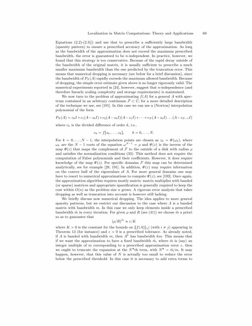
Localization in Matrix Computations: Theory and Applications 69
Equations (2.2)-(2.3)]) and use that to prescribe a sufficiently large bandwidth(sparsity pattern) to ensure a prescribed accuracy of the approximation. As longas the bandwidth of the approximation does not exceed the maximum prescribedbandwidth, the error is guaranteed to be n-independent. In practice, however, wefound that this strategy is too conservative. Because of the rapid decay outside ofthe bandwidth of the original matrix, it is usually sufficient to prescribe a muchsmaller maximum bandwidth than the one predicted by the truncation error. Thismeans that numerical dropping is necessary (see below for a brief discussion), sincethe bandwidth of PN pAq rapidly exceeds the maximum allowed bandwidth. Becauseof dropping, the simple error estimate given above is no longer rigorously valid. Thenumerical experiments reported in [24], however, suggest that n-independence (andtherefore linearly scaling complexity and storage requirements) is maintained.
We now turn to the problem of approximating fpAq for a general A with spec-trum contained in an arbitrary continuum F Ă C; for a more detailed descriptionof the technique we use, see [191]. In this case we can use a (Newton) interpolationpolynomial of the form
PN pAq “ c0I`c1pA´z0Iq`c2pA´z0IqpA´z1Iq`¨ ¨ ¨`cN pA´z0Iq . . . pA´zN´1Iq
where ck is the divided difference of order k, i.e.,
ck “ f rz0, . . . , zks, k “ 0, . . . , N.
For k “ 0, . . . , N ´ 1, the interpolation points are chosen as zk “ Ψpωkq, whereωk are the N ´ 1 roots of the equation ωN´1
“ ρ and Ψpzq is the inverse of themap Φpzq that maps the complement of F to the outside of a disk with radius ρand satisfies the normalization conditions (33). This method does not require thecomputation of Faber polynomials and their coefficients. However, it does requireknowledge of the map Ψpzq. For specific domains F this map can be determinedanalytically, see for example [29, 191]. In addition, Ψpzq may require informationon the convex hull of the eigenvalues of A. For more general domains one mayhave to resort to numerical approximations to compute Ψpzq; see [193]. Once again,the approximation algorithm requires mostly matrix–matrix multiplies with banded(or sparse) matrices and appropriate sparsification is generally required to keep thecost within Opnq as the problem size n grows. A rigorous error analysis that takesdropping as well as truncation into account is however still lacking.
We briefly discuss now numerical dropping. The idea applies to more generalsparsity patterns, but we restrict our discussion to the case where A is a bandedmatrix with bandwidth m. In this case we only keep elements inside a prescribedbandwidth m in every iteration. For given ρ and R (see (41)) we choose m a prioriso as to guarantee that
pρRqm « εK
where K ą 0 is the constant for the bounds on |rfpAqsij | (with i ‰ j) appearing inTheorem 13 (for instance) and ε ą 0 is a prescribed tolerance. As already noted,if A is banded with bandwidth m, then Ak has bandwidth km. This means thatif we want the approximation to have a fixed bandwidth m, where m is (say) aninteger multiple of m corresponding to a prescribed approximation error ε, thenwe ought to truncate the expansion at the N˚th term, with N˚ “ mm. It mayhappen, however, that this value of N is actually too small to reduce the errorbelow the prescribed threshold. In this case it is necessary to add extra terms to

70 Michele Benzi
the Chebyshev expansion; but this would lead to an increase of the bandwidthbeyond the prescribed limit. A solution that has been used by physicists is simplyto continue the recurrence but ignoring all entries in positions outside the prescribedbandwidth; By restricting all the terms in the three-term recurrence (80) to havea fixed bandwidth (independent of n and N) we obtain an approximation schemewhose cost scales linearly in the size n of the problem. This, however, leaves openthe problem of controlling the approximation error.
Approximation based on quadrature rules. Another approach that cansometimes be used to find a banded or sparse approximation of a rapidly decayingmatrix fpAq is based on Gaussian quadrature [95]. With this approach it is possibleto compute or estimate individual entries in fpAq. There exist also block versionsof these techniques which allow the computation of several entries of fpAq at once[95, 171]. Thus, if we know that only the entries of fpAq within a certain bandwidthor block structure are nonnegligible, one can use Gaussian quadrature rules toestimate the entries within this bandwidth or blocks. This approach has been used,e.g., in [22] to construct simple banded preconditioners for Toeplitz matrices withdecay, using the function fpAq “ A´1.
Here we briefly sketch this technique. Suppose f is strictly completely monotonicon an interval pa, bq (see Definition 3). For instance, the function fpxq “ x´σ isstrictly completely monotonic on p0,8q for any σ ą 0, and fpxq “ e´x is strictlycompletely monotonic on R.
Now, let A “ AT P Rnˆn. Consider the eigendecompositions A “ QΛQT andfpAq “ QfpΛqQT . For u,v P Rn we have
uT fpAqv “ uTQfpΛqQTv “ pT fpΛqq “nÿ
i“1
fpλiqpiqi, (82)
where p “ QTu and q “ QTv. In particular, we have that rfpAqsij “ eTi fpAq ej .Next, we rewrite the expression in (82) as a Riemann–Stieltjes integral with
respect to the spectral measure:
uT fpAqv “
ż b
a
fpλqdµpλq, µpλq “
$
&
%
0, if λ ă a “ λ1,řij“1 pjqj , if λi ď λ ă λi`1,
řnj“1 pjqj , if b “ λn ď λ.
The general Gauss-type quadrature rule gives in this case:
ż b
a
fpλqdµpλq “Nÿ
j“1
wjfptjq `Mÿ
k“1
vkfpzkq `Rrf s, (83)
where the nodes ttjuNj“1 and the weights twju
Nj“1 are unknown, whereas the nodes
tzkuMk“1 are prescribed. We have
– M “ 0 for the Gauss rule,– M “ 1, z1 “ a or z1 “ b for the Gauss–Radau rule,– M “ 2, z1 “ a and z2 “ b for the Gauss–Lobatto rule.
Also, for the case u “ v, the remainder in (83) can be written as
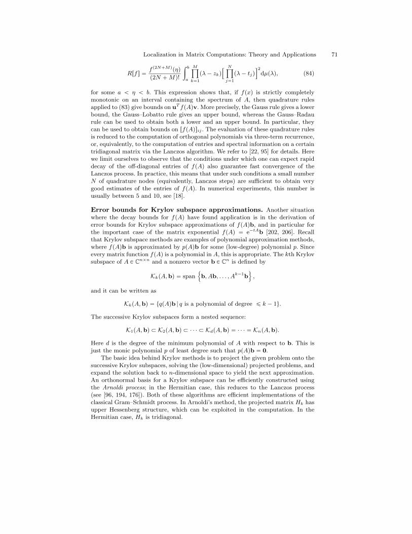
Localization in Matrix Computations: Theory and Applications 71
Rrf s “f p2N`Mqpηq
p2N `Mq!
ż b
a
Mź
k“1
pλ´ zkq”
Nź
j“1
pλ´ tjqı2
dµpλq, (84)
for some a ă η ă b. This expression shows that, if fpxq is strictly completelymonotonic on an interval containing the spectrum of A, then quadrature rulesapplied to (83) give bounds on uT fpAqv. More precisely, the Gauss rule gives a lowerbound, the Gauss–Lobatto rule gives an upper bound, whereas the Gauss–Radaurule can be used to obtain both a lower and an upper bound. In particular, theycan be used to obtain bounds on rfpAqsij . The evaluation of these quadrature rulesis reduced to the computation of orthogonal polynomials via three-term recurrence,or, equivalently, to the computation of entries and spectral information on a certaintridiagonal matrix via the Lanczos algorithm. We refer to [22, 95] for details. Herewe limit ourselves to observe that the conditions under which one can expect rapiddecay of the off-diagonal entries of fpAq also guarantee fast convergence of theLanczos process. In practice, this means that under such conditions a small numberN of quadrature nodes (equivalently, Lanczos steps) are sufficient to obtain verygood estimates of the entries of fpAq. In numerical experiments, this number isusually between 5 and 10, see [18].
Error bounds for Krylov subspace approximations. Another situationwhere the decay bounds for fpAq have found application is in the derivation oferror bounds for Krylov subspace approximations of fpAqb, and in particular forthe important case of the matrix exponential fpAq “ e´tAb [202, 206]. Recallthat Krylov subspace methods are examples of polynomial approximation methods,where fpAqb is approximated by ppAqb for some (low-degree) polynomial p. Sinceevery matrix function fpAq is a polynomial in A, this is appropriate. The kth Krylovsubspace of A P Cnˆn and a nonzero vector b P Cn is defined by
KkpA,bq “ span!
b, Ab, . . . , Ak´1b)
,
and it can be written as
KkpA,bq “ tqpAqb | q is a polynomial of degree ď k ´ 1u.
The successive Krylov subspaces form a nested sequence:
K1pA,bq Ă K2pA,bq Ă ¨ ¨ ¨ Ă KdpA,bq “ ¨ ¨ ¨ “ KnpA,bq.
Here d is the degree of the minimum polynomial of A with respect to b. This isjust the monic polynomial p of least degree such that ppAqb “ 0.
The basic idea behind Krylov methods is to project the given problem onto thesuccessive Krylov subspaces, solving the (low-dimensional) projected problems, andexpand the solution back to n-dimensional space to yield the next approximation.An orthonormal basis for a Krylov subspace can be efficiently constructed usingthe Arnoldi process; in the Hermitian case, this reduces to the Lanczos process(see [96, 194, 176]). Both of these algorithms are efficient implementations of theclassical Gram–Schmidt process. In Arnoldi’s method, the projected matrix Hk hasupper Hessenberg structure, which can be exploited in the computation. In theHermitian case, Hk is tridiagonal.
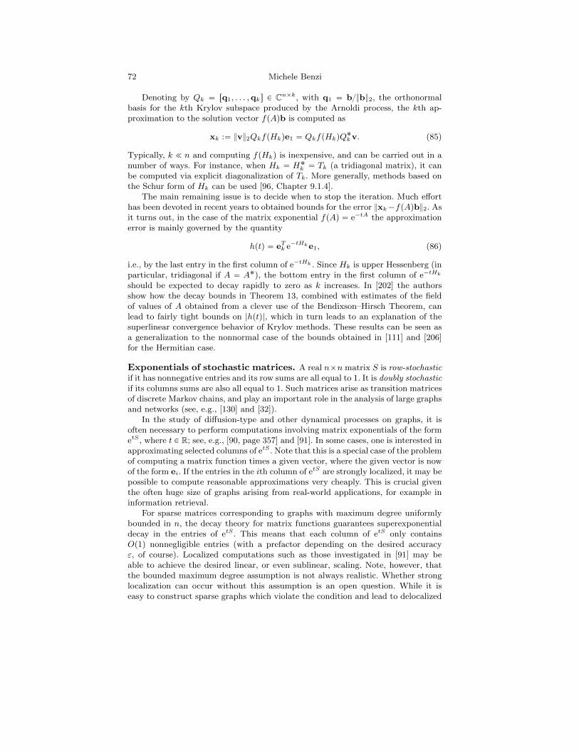
72 Michele Benzi
Denoting by Qk “ rq1, . . . ,qks P Cnˆk, with q1 “ bb2, the orthonormalbasis for the kth Krylov subspace produced by the Arnoldi process, the kth ap-proximation to the solution vector fpAqb is computed as
xk :“ v2QkfpHkqe1 “ QkfpHkqQ˚kv. (85)
Typically, k ! n and computing fpHkq is inexpensive, and can be carried out in anumber of ways. For instance, when Hk “ H˚k “ Tk (a tridiagonal matrix), it canbe computed via explicit diagonalization of Tk. More generally, methods based onthe Schur form of Hk can be used [96, Chapter 9.1.4].
The main remaining issue is to decide when to stop the iteration. Much efforthas been devoted in recent years to obtained bounds for the error xk´fpAqb2. Asit turns out, in the case of the matrix exponential fpAq “ e´tA the approximationerror is mainly governed by the quantity
hptq “ eTk e´tHke1, (86)
i.e., by the last entry in the first column of e´tHk . Since Hk is upper Hessenberg (inparticular, tridiagonal if A “ A˚), the bottom entry in the first column of e´tHk
should be expected to decay rapidly to zero as k increases. In [202] the authorsshow how the decay bounds in Theorem 13, combined with estimates of the fieldof values of A obtained from a clever use of the Bendixson–Hirsch Theorem, canlead to fairly tight bounds on |hptq|, which in turn leads to an explanation of thesuperlinear convergence behavior of Krylov methods. These results can be seen asa generalization to the nonnormal case of the bounds obtained in [111] and [206]for the Hermitian case.
Exponentials of stochastic matrices. A real nˆn matrix S is row-stochasticif it has nonnegative entries and its row sums are all equal to 1. It is doubly stochasticif its columns sums are also all equal to 1. Such matrices arise as transition matricesof discrete Markov chains, and play an important role in the analysis of large graphsand networks (see, e.g., [130] and [32]).
In the study of diffusion-type and other dynamical processes on graphs, it isoften necessary to perform computations involving matrix exponentials of the formetS , where t P R; see, e.g., [90, page 357] and [91]. In some cases, one is interested inapproximating selected columns of etS . Note that this is a special case of the problemof computing a matrix function times a given vector, where the given vector is nowof the form ei. If the entries in the ith column of etS are strongly localized, it may bepossible to compute reasonable approximations very cheaply. This is crucial giventhe often huge size of graphs arising from real-world applications, for example ininformation retrieval.
For sparse matrices corresponding to graphs with maximum degree uniformlybounded in n, the decay theory for matrix functions guarantees superexponentialdecay in the entries of etS . This means that each column of etS only containsOp1q nonnegligible entries (with a prefactor depending on the desired accuracyε, of course). Localized computations such as those investigated in [91] may beable to achieve the desired linear, or even sublinear, scaling. Note, however, thatthe bounded maximum degree assumption is not always realistic. Whether stronglocalization can occur without this assumption is an open question. While it iseasy to construct sparse graphs which violate the condition and lead to delocalized
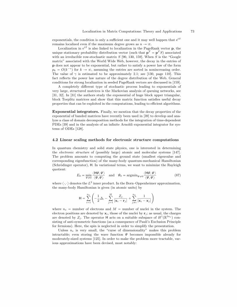
Localization in Matrix Computations: Theory and Applications 73
exponentials, the condition is only a sufficient one and it may well happen that etS
remains localized even if the maximum degree grows as nÑ8.Localization in etS is also linked to localization in the PageRank vector p, the
unique stationary probability distribution vector (such that pT “ pTS) associatedwith an irreducible row-stochastic matrix S [90, 130, 159]. When S is the “Googlematrix” associated with the World Wide Web, however, the decay in the entries ofp does not appear to be exponential, but rather to satisfy a power law of the formpk “ Opk´γq for k Ñ 8, assuming the entries are sorted in nonincreasing order.The value of γ is estimated to be approximately 2.1; see [130, page 110]. Thisfact reflects the power law nature of the degree distribution of the Web. Generalconditions for strong localization in seeded PageRank vectors are discussed in [159].
A completely different type of stochastic process leading to exponentials ofvery large, structured matrices is the Markovian analysis of queuing networks, see[31, 32]. In [31] the authors study the exponential of huge block upper triangular,block Toeplitz matrices and show that this matrix function satisfies useful decayproperties that can be exploited in the computations, leading to efficient algorithms.
Exponential integrators. Finally, we mention that the decay properties of theexponential of banded matrices have recently been used in [39] to develop and ana-lyze a class of domain decomposition methods for the integration of time-dependentPDEs [39] and in the analysis of an infinite Arnoldi exponential integrator for sys-tems of ODEs [128].
4.2 Linear scaling methods for electronic structure computations
In quantum chemistry and solid state physics, one is interested in determiningthe electronic structure of (possibly large) atomic and molecular systems [147].The problem amounts to computing the ground state (smallest eigenvalue andcorresponding eigenfunction) of the many-body quantum-mechanical Hamiltonian(Schrodinger operator), H. In variational terms, we want to minimize the Rayleighquotient:
E0 “ minΨ‰0
xHΨ, Ψy
xΨ, Ψyand Ψ0 “ argminΨ‰0
xHΨ, Ψy
xΨ, Ψy(87)
where x¨, ¨y denotes the L2 inner product. In the Born–Oppenheimer approximation,the many-body Hamiltonian is given (in atomic units) by
H “neÿ
i“1
˜
´1
2∆i ´
Mÿ
j“1
Zj|xi ´ rj |
`
neÿ
j‰i
1
|xi ´ xj |
¸
where ne “ number of electrons and M “ number of nuclei in the system. Theelectron positions are denoted by xi, those of the nuclei by rj ; as usual, the chargesare denoted by Zj . The operator H acts on a suitable subspace of H1
pR3neq con-sisting of anti-symmetric functions (as a consequence of Pauli’s Exclusion Principlefor fermions). Here, the spin is neglected in order to simplify the presentation.
Unless ne is very small, the “curse of dimensionality” makes this problemintractable; even storing the wave function Ψ becomes impossible already formoderately-sized systems [125]. In order to make the problem more tractable, var-ious approximations have been devised, most notably:

74 Michele Benzi
– Wave function methods (e.g., Hartree–Fock);– Density Functional Theory (e.g., Kohn-Sham);– Hybrid methods (e.g., B3LYP).
In these approximations the original, linear eigenproblem HΨ “ EΨ for the many-electrons Hamiltonian is replaced by a non-linear one-particle eigenproblem:
Fpψiq “ λiψi, xψi, ψjy “ δij , 1 ď i, j ď ne, (88)
where λ1 ď λ2 ď ¨ ¨ ¨ ď λne are the ne smallest eigenvalues of (88). In the case ofDensity Functional Theory, (88) are known as the Kohn–Sham equations, and thenonlinear operator F in (88) has the form Fpψiq “
`
´ 12∆` V pρq
˘
ψi, where ρ “ρpxq “
řnei“1 |ψipxq|
2 is a the electronic density, a function of only three variablesthat alone is sufficient to determine, in principle, all the properties of a system[112, 126]. The Kohn–Sham equations (88) are the Euler–Lagrange equations for theminimization of a functional J “ Jrρs (the density functional) such that the groundstate energy, E0, is the minimum of the functional: E0 “ infρ J . While the exactform of this functional is not known explicitly, a number of increasingly accurateapproximations have been developed since the original paper [126] appeared. Theenormous success of Density Functional Theory (which led to the award of a shareof the 1998 Nobel Prize for Chemistry to Kohn) is due to the fact that the high-dimensional, intractable minimization problem (87) with respect to Ψ P L2
pR3neq
is replaced by a minimization problem with respect to ρ P L2pR3q.
The nonlinear Kohn–Sham equations (88) can be solved by a “self-consistentfield” (SCF) iteration, leading to a sequence of linear eigenproblems
F pkqψpkqi “ λpkqi ψ
pkqi , xψ
pkqi , ψ
pkqj y “ δij , k “ 1, 2, . . . (89)
(1 ď i, j ď ne), where each F pkq “ ´ 12∆` V pkq is a one-electron Hamiltonian with
potential
V pkq “ V pkqpρpk´1qq, ρpk´1q
“
neÿ
i“1
|ψpk´1qi pxq|2.
Solution of each of the (discretized) linear eigenproblems (89) leads to a typ-
ical Opn3eq cost per SCF iteration. However, the actual eigenpairs pψ
pkqi , λ
pkqi q are
unnecessary; hence, diagonalization of the (discretized) one-particle Hamiltonianscan be avoided. Indeed, all one really needs is the density matrix, i.e., the spectralprojector P onto the invariant subspace
Vocc “ spantψ1, . . . , ψneu
corresponding to the ne lowest eigenvalues λ1 ď λ2 ď ¨ ¨ ¨ ď λne (“occupied states”).At the kth SCF cycle, an approximation P pkq « P to the orthogonal projector ontothe occupied subspace Vocc needs to be computed. At convergence, all quantities ofinterest in electronic structure theory can be computed from P .
In practice, operators are replaced by matrices by Galerkin projection onto afinite-dimensional subspace spanned by a set of basis functions tφiu
ni“1, where n
is a multiple of ne. Typically, n “ nb ¨ ne where nb ě 2 is a moderate constantwhen linear combinations of Gaussian-type orbitals are used; often, nb « 10 ´ 25(see [134]). We assume that the basis functions are localized, so that the resultingdiscrete Hamiltonians (denoted by H) are, up to some small truncation tolerance,
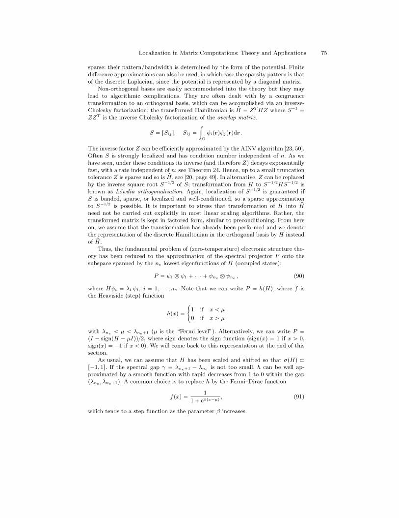
Localization in Matrix Computations: Theory and Applications 75
sparse: their pattern/bandwidth is determined by the form of the potential. Finitedifference approximations can also be used, in which case the sparsity pattern is thatof the discrete Laplacian, since the potential is represented by a diagonal matrix.
Non-orthogonal bases are easily accommodated into the theory but they maylead to algorithmic complications. They are often dealt with by a congruencetransformation to an orthogonal basis, which can be accomplished via an inverse-Cholesky factorization; the transformed Hamiltonian is pH “ ZTHZ where S´1
“
ZZT is the inverse Cholesky factorization of the overlap matrix,
S “ rSijs, Sij “
ż
Ω
φiprqφjprqdr .
The inverse factor Z can be efficiently approximated by the AINV algorithm [23, 50].Often S is strongly localized and has condition number independent of n. As wehave seen, under these conditions its inverse (and therefore Z) decays exponentiallyfast, with a rate independent of n; see Theorem 24. Hence, up to a small truncationtolerance Z is sparse and so is pH, see [20, page 49]. In alternative, Z can be replacedby the inverse square root S´12 of S; transformation from H to S´12HS´12 isknown as Lowdin orthogonalization. Again, localization of S´12 is guaranteed ifS is banded, sparse, or localized and well-conditioned, so a sparse approximationto S´12 is possible. It is important to stress that transformation of H into pHneed not be carried out explicitly in most linear scaling algorithms. Rather, thetransformed matrix is kept in factored form, similar to preconditioning. From hereon, we assume that the transformation has already been performed and we denotethe representation of the discrete Hamiltonian in the orthogonal basis by H insteadof pH.
Thus, the fundamental problem of (zero-temperature) electronic structure the-ory has been reduced to the approximation of the spectral projector P onto thesubspace spanned by the ne lowest eigenfunctions of H (occupied states):
P “ ψ1 b ψ1 ` ¨ ¨ ¨ ` ψne b ψne , (90)
where Hψi “ λi ψi, i “ 1, . . . , ne. Note that we can write P “ hpHq, where f isthe Heaviside (step) function
hpxq “
#
1 if x ă µ
0 if x ą µ
with λne ă µ ă λne`1 (µ is the “Fermi level”). Alternatively, we can write P “
pI ´ signpH ´ µIqq2, where sign denotes the sign function (signpxq “ 1 if x ą 0,signpxq “ ´1 if x ă 0). We will come back to this representation at the end of thissection.
As usual, we can assume that H has been scaled and shifted so that σpHq Ăr´1, 1s. If the spectral gap γ “ λne`1 ´ λne is not too small, h can be well ap-proximated by a smooth function with rapid decreases from 1 to 0 within the gappλne , λne`1q. A common choice is to replace h by the Fermi–Dirac function
fpxq “1
1` eβpx´µq, (91)
which tends to a step function as the parameter β increases.

76 Michele Benzi
Physicists have observed long ago that for “gapped systems” (like insulatorsand, under certain conditions, semiconductors) the entries of the density matrixP decay exponentially fast away from the main diagonal, reflecting the fact thatinteraction strengths decrease rapidly with the distance [9, 70, 107, 118, 123, 134,148, 160, 167, 169]. We recall that, as already discussed, exponential decay in theψi in (90) is sufficient for localization of the density matrix P , but not necessary;and indeed, situations can be found where P decays exponentially but the ψi donot, see [45] and the discussion in [20, section 4].
Localization of the density matrix is a manifestation of the “nearsightedness”of electronic matter discussed in section 1.1.15 Localization is crucial as it providesthe basis for so-called linear scaling (i.e., Opneq) methods for electronic structurecalculations. These methods have been vigorously developed since the early 1990s,and they are currently able to handle very large systems, see, e.g., [9, 10, 37, 43, 50,92, 124, 132, 135, 136, 139, 161, 174, 177, 205]. These methods including expansionof the Fermi–Dirac operator fpHq in the Chebyshev basis, constrained optimizationmethods based on density matrix minimization (possibly with `1 regularization toenforce localized solutions), methods based on the sign matrix representation ofP (such as “McWeeny purification”), multipole expansions, and many others. Aswe have seen, rapidly decaying matrices can be approximated by sparse matrices,uniformly in n. Hence, rigorously establishing the rate of decay in the densitymatrix provides a sound mathematical foundation for linear scaling methods inelectronic structure calculations. A mathematical analysis of the asymptotic decayproperties of spectral projectors associated with large, banded or sparse Hermitianmatrices has been presented in [20]. The main result in [20] can be summarized inthe following theorem.
Theorem 26. ([20]) Let n “ nb ¨ ne where nb is a fixed positive integer and theintegers ne form a monotonically increasing sequence. Let tHnu be a sequence ofHermitian nˆ n matrices with the following properties:
1. Each Hn has bandwidth m independent of n;2. There exist two (fixed) intervals I1 “ ra, bs, I2 “ rc, ds Ă R with γ “ c ´ b ą
0 such that for all n “ nb ¨ ne, I1 contains the smallest ne eigenvalues ofHn (counted with their multiplicities) and I2 contains the remaining n ´ neeigenvalues.
Let Pn denote the nˆ n spectral projector onto the subspace spanned by the eigen-vectors associated with the ne smallest eigenvalues of Hn, for each n. Then thereexist constants K ą 0, α ą 0 independent of n such that
|rPnsij | ď K e´α|i´j|, @i ‰ j. (92)
Moreover, for any ε ą 0 there is a matrix Pn of bandwidth p independent of n suchthat Pn ´ Pn ă ε, for all n.
15 As we saw earlier (see (79)), rapid decay in P means that quantities like TrpPHq,which in electronic structure theory has the interpretation of a single particle-energy [92, 161], are insensitive to small perturbations in the Hamiltonian inpositions that correspond to small entries in P . Also, the fact that TrpP q “rankpP q “ ne ! n implies that many of the diagonal entries of P will be tiny;hence, slight changes in the potential V pxq at a point x are only felt locally, seeExample 2.

Localization in Matrix Computations: Theory and Applications 77
As usual, the bandedness assumption can be replaced with the assumptionthat the Hamiltonians are sparse, with associated graphs that satisfy the boundedmaximum degree assumption. In this case the geodesic distance on the graphsshould be used to measure decay.
Different proofs of Theorem 26 can be found in [20]. One approach consistsin approximating Pn via the (analytic) Fermi–Dirac function (91), and exploitingthe fact that the rate of decay in fpHnq is independent of n thanks to the non-vanishing gap assumption. This approach yields explicit, computable formulas forthe constants K and α in (92), see [20, pages 26–27]. Another approach is based onresults on the polynomial approximation of analytic functions on disjoint intervals[59, 105]. Both proofs make crucial use of the general theory of exponential decayin analytic functions of banded and sparse matrices discussed earlier, in particularTheorem 9.
Some comments about the meaning of Theorem 26 are in order. The first thingto observe is that the independence of the decay bounds on n follows from theassumption that n “ nb ¨ne where nb, which controls the accuracy of the discretiza-tion, is fixed, whereas ne, which determines the system size (i.e., the number ofelectrons in the system), is allowed to increase without bounds. This is sometimesreferred to as the thermodynamic limit, where the system size grows but the dis-tance between atoms is kept constant. It should not be confused with the limit inwhich ne is fixed and nb Ñ 8, or with the case where both ne and nb are allowedto grow without bounds. Keeping nb constant ensures that the spectra of the dis-crete Hamiltonians remain uniformly bounded, which guarantees (for insulators)that the relative spectral gap γ does not vanish as n Ñ 8. In practice a constantnb is a reasonable assumption since existing basis sets are not very large and theyare already highly optimized so as to achieve the desired accuracy.
Another issue that warrants comment is the choice of the parameter β (the“inverse temperature”) in the Fermi–Dirac function. Note that the Fermi–Diracfunction has two poles in the complex plane: if we assume, without loss of generality,that the Fermi level is at µ “ 0, the poles are on the imaginary axis at ˘iπβ.Since the rate of decay is governed by the distance between these two poles andthe smallest intervals I1, I2 containing all the spectra σpHnq, a large value of β(corresponding to a small gap γ) means that the poles approach 0 and therefore band c. In this case, decay could be slow; indeed, the rate of decay α in the bounds(92) tends to zero as γ Ñ 0 or, equivalently, as β Ñ 8. On the other hand, arelatively large value of γ means that β can be chosen moderate and this will implyfast decay in the entries of the density matrix Pn, for all n. We refer to [20, pages40–42] for details on the dependence of the decay rate in the density matrix as afunction of the gap and of the temperature, in particular in the zero-temperaturelimit (β Ñ 8), and to [190] for an example of how these results can be used inactual computations.
The case of metallic systems at zero temperature corresponds to γ Ñ 0. In thiscase the bound (92) becomes useless, since αÑ 0. The actual decay in the densitymatrix in this case can be as slow as p1`|i´j|q´1; see [20, section 10] for a detailedanalysis of a model problem.
We conclude this section discussing alternative representations of the densitymatrix that could potentially lead to better decay bounds. Recall that the step func-tion hpxq can be expressed in terms of the sign function as hpxq “ p1´ signpxqq2.

78 Michele Benzi
Hence, studying the decay behavior of the spectral projector hpHq amounts tostudying the decay behavior in signpHq. Again, we assume for simplicity that theFermi level is at µ “ 0. Now, the matrix sign function admits a well known integralrepresentation, see [109]:
signpHq “2
πH
ż 8
0
pt2I `H2q´1dt. (93)
One can now use available decay bounds on the inverse of the banded (or sparse)Hermitian positive definite matrix t2I`H2 together with quadrature rules to obtainbounds on the entries of signpHq and therefore of P . Note the similarity of thisapproach with the one reviewed in section 3.5.
Another approach, which yields more explicit bounds, is based on the identity
signpHq “ HpH2q´12, (94)
see again [109]. We can then use bounds for the inverse square root of the banded (orsparse) Hermitian positive definite matrix H2 to obtain exponential decay boundsfor signpHq, using the fact that the product of a banded (or sparse) matrix timesan exponentially decaying one retains the exponential decay property. Preliminarynumerical experiments on simple model gapped Hamiltonians [38] suggest that thedecay bounds obtained via the representations (93) and (94) can be more accuratethan those obtained via the Fermi–Dirac representation.
4.3 Further applications
In this section we briefly mention a few other applications of localization and decaybounds in applied mathematics and physics.
Localized solutions to matrix equations. In the area of control of discrete-time, large-scale dynamical systems, a central role is played by the Lyapunov equa-tion associated to a linear, time-varying dynamical system:
AX `XAT “ P, (95)
with A,P P Rnˆn given matrices and X unknown. If A is stable, equation (95) hasa unique solution, which can be expressed as
X “ ´
ż 8
0
etAP etA dt ; (96)
and also as the solution of a linear system in Kronecker sum form:
pI bA`AT b IqvecpXq “ vecpP q , (97)
where “vec” is the operator that takes an n ˆ n matrix and forms the vector oflength n2 consisting of the columns of the matrix stacked one on top of one another;see, e. g. [131] or [183].
Several authors (e.g., [52, 104]) have observed that whenever A and P arebanded, or sparse, the solution matrix X is localized, with rapid off-diagonal decayif A is well-conditioned. Moreover, the decay is oscillatory (see [104, Fig. 3]). This

Localization in Matrix Computations: Theory and Applications 79
does not come as a surprise given the relation of X to the matrix exponential ofA, see (96), and to the inverse of a matrix in Kronecker sum form, see (97). Thedecay in the solution has been exploited to develop efficient solution techniquesfor (95) with A and P banded. When A “ AT , an approximate solution to (95)can sometimes be obtained using polynomial expansion in the Chebyshev basis, asoutlined in the previous section. We refer again to [104] for details.
Localized matrices (in the form of rapidly decaying inverse Gramians) also arisein another problem in control theory, namely, subspace identification of large-scaleinterconnected systems. Again, this fact can be exploited to develop fast approxi-mation algorithms; see [103].
For a different application of exponential decay bounds for A´1 to the study ofthe behavior of dynamical systems, see [155].
Localization in graph and network analysis. Recently, several authorshave proved that, with high probability, the eigenvectors of the adjacency matrix[66, 74, 192] and of the Laplacian [44] of large sparse undirected random graphs, inparticular Erdos–Renyi graphs, are delocalized, a fact that was already known onthe basis of empirical observation; see, e.g., [94]. On the other hand, localization ineigenvectors of scale-free networks, particularly those corresponding to the largesteigenvalues of the adjacency matrix or of the Laplacian, has been reported, forboth synthetic [94, 151] and real-world [108, 158, 180] networks. For instance, in[94] the eigenvector corresponding to the largest eigenvalue of the adjacency matrixof a power-law graph was found to be localized at the hub (the node of maximumdegree).
Power-law graphs are also studied in [108], where a class of graph substruc-tures leading to locally supported eigenvectors is identified. In some cases theseeigenvectors are actually sparse, not just localized: an extreme example is givenby the so-called Faria vectors [83], i.e., eigenvectors that have only two nonzerocomponents (one positive, the other necessarily negative). These eigenvectors areassociated with eigenvalues of very high multiplicity (sometimes as large as Opnq),such as those associated with star graphs—graphs consisting of a central node con-nected to several peripheral nodes. Many star-like subgraphs, and thus Laplacianeigenvalues of very high multiplicity, are often found in real-world scale-free graphs,an observation that leads to the conjecture that such Laplacians may have a numberof locally supported eigenvectors. We refer to [108] for a detailed study, includingcomputational aspects. It should be noted that since power-law graphs do not sat-isfy the bounded maximum degree assumption, we cannot directly apply the decaytheory for matrix functions (and in particular for spectral projectors) to explainthe eigenvector localization discussed in [94, 108].
Another class of graphs for which eigenvector localization has been observedis discussed in [158], motivated by the study of dendrites of retinal ganglion cells(RGCs). It turns out the Laplacian eigenvalues of a typical dendritic tree displaya peculiar distribution: most of the λi are distributed according to a smooth curvein the interval p0, 4q, after which a jump occurs in the spectrum and the remainingeigenvalues are clustered around some value larger than 4. Moreover, the eigenvec-tors associated with eigenvalues less than 4 are delocalized, while those associatedwith eigenvalues greater than 4 are exponentially localized.
In order to find an explanation to this phenomenon, the authors of [158] considersimplified models of RGCs that are easier to analyze but at the same time capture

80 Michele Benzi
the main properties of RGCs. The simplest among these models is a star-like tree,obtained by connecting one or more path graphs to the central hub of a star graphSk (consisting of k peripheral nodes connected to a central node), where k ě 3. Inthe case of a single path graph P` connected to the central hub of a star graph Sk,the resulting graph is called a comet of type pk, `q. The Laplacian of the resultingstar-like tree is then obtained by gluing the Laplacians of Sk and P` For example,in the case k “ 4, ` “ 5 the corresponding comet graph (with the hub numberedfirst) has 10 nodes and the associated Laplacian is given by
L “
»
—
—
—
—
—
—
—
—
—
—
—
—
—
—
–
5 ´1 ´1 ´1 ´1 ´1 0 0 0 0´1 1 0 0 0 0 0 0 0 0´1 0 1 0 0 0 0 0 0 0´1 0 0 1 0 0 0 0 0 0´1 0 0 0 1 0 0 0 0 0
´1 0 0 0 0 2 ´1 0 0 00 0 0 0 0 ´1 2 ´1 0 00 0 0 0 0 0 ´1 2 ´1 00 0 0 0 0 0 0 ´1 2 ´10 0 0 0 0 0 0 0 ´1 1
fi
ffi
ffi
ffi
ffi
ffi
ffi
ffi
ffi
ffi
ffi
ffi
ffi
ffi
ffi
fl
,
where the horizontal and vertical line have been added to more clearly show howthe gluing of the Laplacians of S4 and P5 is carried out. The resulting L has nineeigenvalues ă 4, all falling between 0 and 3.652007105, with the tenth eigenvalueλ « 6.0550. It is known that a star-like tree can have only one eigenvalue ě 4, withequality if and only if the graph is a claw (see [158] for details). In our example the(normalized) eigenvector associated with the largest eigenvalue is of the form
v ““
v1, v2
‰
,
wherev1 “
“
0.9012, ´0.1783, ´0.1783, ´0.1783, ´0.1783‰
,
andv2 “
“
0.2377, ´0.0627, 0.0165, ´0.0043, 0.0008‰
(rounding to four decimal places). We see that the dominant eigenvector is mostlyconcentrated at the hub, is constant on the peripheral nodes of the star S4, anddecays monotonically in magnitude along the path P5 away from the hub. It canbe shown that this phenomenon is common to all comet graphs and that the decayof the dominant eigenvector along the path is exponential [158]. Moreover, similarbehavior is also common to star-like trees in general; if there are multiple pathsconnected to the central node of a star, the dominant eigenvector will decay ex-ponentially along the paths, away from the central hub, where the eigenvector isconcentrated. The remaining eigenvectors, corresponding to eigenvalues less than4, are delocalized (oscillatory).
The proofs in [158] are direct and are based on previous results on the eigen-values of star-like trees, together with a careful analysis of certain recurrences thatthe entries of the dominant eigenvector of L must satisfy. Here we point out thatthe decay behavior of the dominant eigenvector of L for star-like trees (and alsofor more general, less structured graphs obtained by gluing one or more long pathsto a graph having a hub of sufficiently high degree) is a byproduct of our general

Localization in Matrix Computations: Theory and Applications 81
decay results for functions of banded or sparse matrices. To see this, we considerthe case of a single path of length ` attached to the hub of a graph with order k`1nodes. The resulting graph has n “ k` ``1 nodes, and its Laplacian is of the form
Ln “
„
L11 L12
LT12 L22
,
where L12 is a pk ` 1q ˆ ` matrix with all its entries equal to 0 except for a ´1 inthe upper left corner. For fixed k and increasing `, the sequence tLnu satisfies theassumptions of Theorem 9, therefore for any analytic function f , the entries of fpLnqmust decay at least exponentially fast away from the main diagonal (or nonzeropattern of Ln) with rate independent of n for ` sufficiently large. Moreover, assumethat the dominant eigenvalue of Ln is well separated from the rest of the spectrum;this happens for example if one of the nodes, say the first, has a significantly higherdegree than the remaining ones. Then the corresponding eigenvector is localized,and its entries decay exponentially along the path, away from the hub. To see thiswe can approximate the corresponding spectral projector, P , by a Gaussian in Lnand use the fact that TrpP q “ 1, as discussed earlier.
Next, we consider the issue of localization in functions of matrices associatedwith graphs, limited to the undirected case. We are especially interested in thematrix exponential, which is widely used in the study of network structure anddynamics. We discuss first the communicability between nodes, see (7), which ismeasured by the entries of the exponential of the adjacency matrix. In many ap-plications, see for example [81], it is desirable to identify pairs of nodes within anetwork having low communicability. For fairly regular sparse graphs with largediameter, communication between neighboring nodes is clearly much easier thancommunication between pairs of distant nodes, and this fact is well captured bythe fact that reAsij decays superexponentially with the geodesic distance dpi, jq.The simplest example is that of a path graph P`, for which A is tridiagonal: aswe have shown, in this case the entries of the exponential decay very fast with thedistance |i ´ j|. On the other hand, for large connected graphs of small diameter,like many real world complex networks, the distance dpi, jq is small for any i andj, and decay bounds like (29) cannot predict any small entries in functions of theadjacency matrix. This fact is related to the violation of the bounded maximumdegree assumption. The simplest example is now that of a star graph Sn, which hasdiameter 2 and maximum degree n, and for which there is no decay whatsoever ineA.
Analogous remarks apply to functions of the Laplacian of a connected graph.Consider for instance the heat kernel, e´tL. As is well known, this matrix functionoccurs in the solution of initial value problems of the form
9x “ ´Lx subject to xp0q “ x0, (98)
where the dot on a vector denotes differentiation with respect to time and x0 P Rnis given. The solution of (98) is given, for all t ě 0, by
xptq “ e´tLx0.
Consider now the special case where x0 “ ei, the ith vector of the standard basis.This means that a unit amount of some “substance” is placed at node i at time
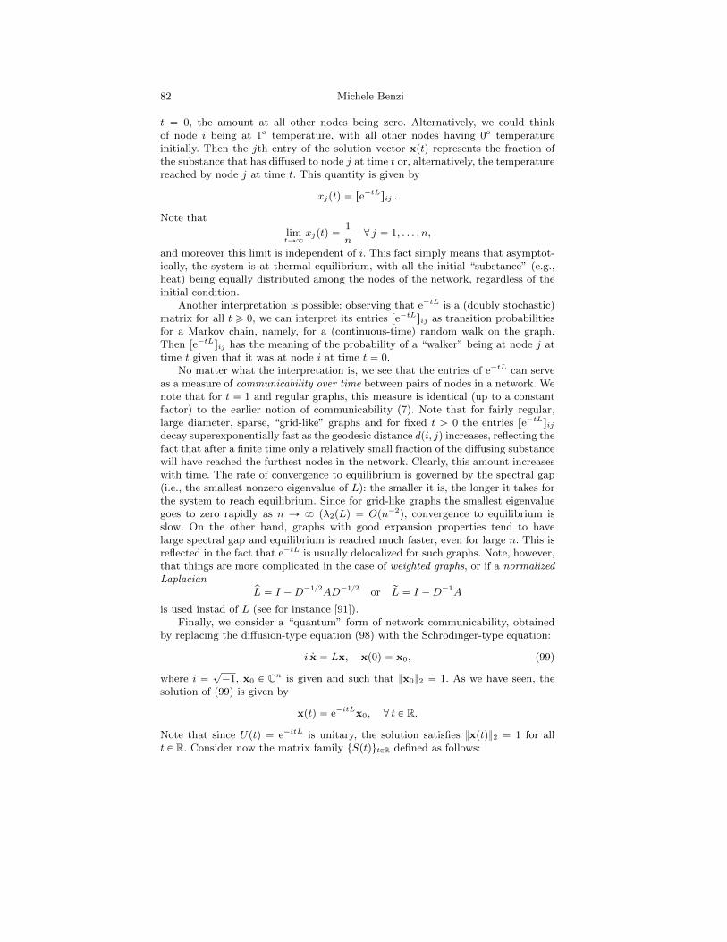
82 Michele Benzi
t “ 0, the amount at all other nodes being zero. Alternatively, we could thinkof node i being at 1o temperature, with all other nodes having 0o temperatureinitially. Then the jth entry of the solution vector xptq represents the fraction ofthe substance that has diffused to node j at time t or, alternatively, the temperaturereached by node j at time t. This quantity is given by
xjptq “ re´tLsij .
Note that
limtÑ8
xjptq “1
n@ j “ 1, . . . , n,
and moreover this limit is independent of i. This fact simply means that asymptot-ically, the system is at thermal equilibrium, with all the initial “substance” (e.g.,heat) being equally distributed among the nodes of the network, regardless of theinitial condition.
Another interpretation is possible: observing that e´tL is a (doubly stochastic)matrix for all t ě 0, we can interpret its entries re´tLsij as transition probabilitiesfor a Markov chain, namely, for a (continuous-time) random walk on the graph.Then re´tLsij has the meaning of the probability of a “walker” being at node j attime t given that it was at node i at time t “ 0.
No matter what the interpretation is, we see that the entries of e´tL can serveas a measure of communicability over time between pairs of nodes in a network. Wenote that for t “ 1 and regular graphs, this measure is identical (up to a constantfactor) to the earlier notion of communicability (7). Note that for fairly regular,large diameter, sparse, “grid-like” graphs and for fixed t ą 0 the entries re´tLsijdecay superexponentially fast as the geodesic distance dpi, jq increases, reflecting thefact that after a finite time only a relatively small fraction of the diffusing substancewill have reached the furthest nodes in the network. Clearly, this amount increaseswith time. The rate of convergence to equilibrium is governed by the spectral gap(i.e., the smallest nonzero eigenvalue of L): the smaller it is, the longer it takes forthe system to reach equilibrium. Since for grid-like graphs the smallest eigenvaluegoes to zero rapidly as n Ñ 8 (λ2pLq “ Opn´2), convergence to equilibrium isslow. On the other hand, graphs with good expansion properties tend to havelarge spectral gap and equilibrium is reached much faster, even for large n. This isreflected in the fact that e´tL is usually delocalized for such graphs. Note, however,that things are more complicated in the case of weighted graphs, or if a normalizedLaplacian
pL “ I ´D´12AD´12 or rL “ I ´D´1A
is used instad of L (see for instance [91]).Finally, we consider a “quantum” form of network communicability, obtained
by replacing the diffusion-type equation (98) with the Schrodinger-type equation:
i 9x “ Lx, xp0q “ x0, (99)
where i “?´1, x0 P Cn is given and such that x02 “ 1. As we have seen, the
solution of (99) is given by
xptq “ e´itLx0, @ t P R.
Note that since Uptq “ e´itL is unitary, the solution satisfies xptq2 “ 1 for allt P R. Consider now the matrix family tSptqutPR defined as follows:
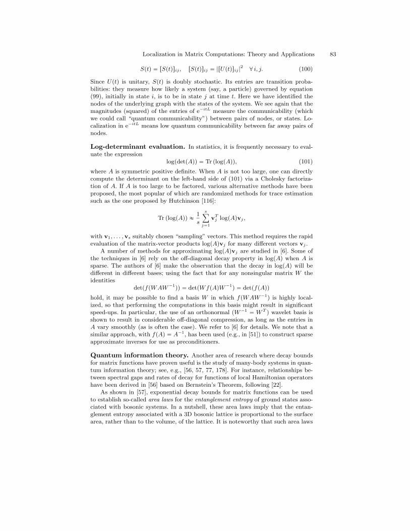
Localization in Matrix Computations: Theory and Applications 83
Sptq “ rSptqsij , rSptqsij “ |rUptqsij |2@ i, j. (100)
Since Uptq is unitary, Sptq is doubly stochastic. Its entries are transition proba-bilities: they measure how likely a system (say, a particle) governed by equation(99), initially in state i, is to be in state j at time t. Here we have identified thenodes of the underlying graph with the states of the system. We see again that themagnitudes (squared) of the entries of e´itL measure the communicability (whichwe could call “quantum communicability”) between pairs of nodes, or states. Lo-calization in e´itL means low quantum communicability between far away pairs ofnodes.
Log-determinant evaluation. In statistics, it is frequently necessary to eval-uate the expression
logpdetpAqq “ Tr plogpAqq, (101)
where A is symmetric positive definite. When A is not too large, one can directlycompute the determinant on the left-hand side of (101) via a Cholesky factoriza-tion of A. If A is too large to be factored, various alternative methods have beenproposed, the most popular of which are randomized methods for trace estimationsuch as the one proposed by Hutchinson [116]:
Tr plogpAqq «1
s
sÿ
j“1
vTj logpAqvj ,
with v1, . . . ,vs suitably chosen “sampling” vectors. This method requires the rapidevaluation of the matrix-vector products logpAqvj for many different vectors vj .
A number of methods for approximating logpAqvj are studied in [6]. Some ofthe techniques in [6] rely on the off-diagonal decay property in logpAq when A issparse. The authors of [6] make the observation that the decay in logpAq will bedifferent in different bases; using the fact that for any nonsingular matrix W theidentities
detpfpWAW´1qq “ detpWfpAqW´1
q “ detpfpAqq
hold, it may be possible to find a basis W in which fpWAW´1q is highly local-
ized, so that performing the computations in this basis might result in significantspeed-ups. In particular, the use of an orthonormal (W´1
“ WT ) wavelet basis isshown to result in considerable off-diagonal compression, as long as the entries inA vary smoothly (as is often the case). We refer to [6] for details. We note that asimilar approach, with fpAq “ A´1, has been used (e.g., in [51]) to construct sparseapproximate inverses for use as preconditioners.
Quantum information theory. Another area of research where decay boundsfor matrix functions have proven useful is the study of many-body systems in quan-tum information theory; see, e.g., [56, 57, 77, 178]. For instance, relationships be-tween spectral gaps and rates of decay for functions of local Hamiltonian operatorshave been derived in [56] based on Bernstein’s Theorem, following [22].
As shown in [57], exponential decay bounds for matrix functions can be usedto establish so-called area laws for the entanglement entropy of ground states asso-ciated with bosonic systems. In a nutshell, these area laws imply that the entan-glement entropy associated with a 3D bosonic lattice is proportional to the surfacearea, rather than to the volume, of the lattice. It is noteworthy that such area laws
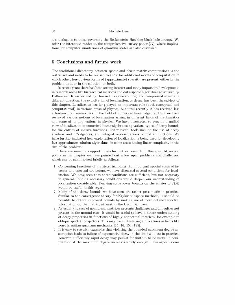
84 Michele Benzi
are analogous to those governing the Beckenstein–Hawking black hole entropy. Werefer the interested reader to the comprehensive survey paper [77], where implica-tions for computer simulations of quantum states are also discussed.
5 Conclusions and future work
The traditional dichotomy between sparse and dense matrix computations is toorestrictive and needs to be revised to allow for additional modes of computation inwhich other, less-obvious forms of (approximate) sparsity are present, either in theproblem data or in the solution, or both.
In recent years there has been strong interest and many important developmentsin research areas like hierarchical matrices and data-sparse algorithms (discussed byBallani and Kressner and by Bini in this same volume) and compressed sensing; adifferent direction, the exploitation of localization, or decay, has been the subject ofthis chapter. Localization has long played an important role (both conceptual andcomputational) in various areas of physics, but until recently it has received lessattention from researchers in the field of numerical linear algebra. Here we havereviewed various notions of localization arising in different fields of mathematicsand some of its applications in physics. We have attempted to provide a unifiedview of localization in numerical linear algebra using various types of decay boundsfor the entries of matrix functions. Other useful tools include the use of decayalgebras and C˚-algebras, and integral representations of matrix functions. Wehave further indicated how exploitation of localization is being used for developingfast approximate solution algorithms, in some cases having linear complexity in thesize of the problem.
There are numerous opportunities for further research in this area. At severalpoints in the chapter we have pointed out a few open problems and challenges,which can be summarized briefly as follows.
1. Concerning functions of matrices, including the important special cases of in-verses and spectral projectors, we have discussed several conditions for local-ization. We have seen that these conditions are sufficient, but not necessaryin general. Finding necessary conditions would deepen our understanding oflocalization considerably. Deriving some lower bounds on the entries of fpAqwould be useful in this regard.
2. Many of the decay bounds we have seen are rather pessimistic in practice.Similar to the convergence theory for Krylov subspace methods, it should bepossible to obtain improved bounds by making use of more detailed spectralinformation on the matrix, at least in the Hermitian case.
3. As usual, the case of nonnormal matrices presents challenges and difficulties notpresent in the normal case. It would be useful to have a better understandingof decay properties in functions of highly nonnormal matrices, for example inoblique spectral projectors. This may have interesting applications in fields likenon-Hermitian quantum mechanics [15, 16, 154, 195].
4. It is easy to see with examples that violating the bounded maximum degree as-sumption leads to failure of exponential decay in the limit nÑ8; in practice,however, sufficiently rapid decay may persist for finite n to be useful in com-putation if the maximum degree increases slowly enough. This aspect seems

Localization in Matrix Computations: Theory and Applications 85
to warrant further investigation, especially in view of applications in networkanalysis.
5. It would be interesting to develop general conditions under which boundedfunctions of unbounded, banded operators (or sequences of banded finite ma-trices without uniformly bounded spectra) exhibit decay behavior.
6. Outside of the broad area of linear scaling methods for electronic structurecomputations and in the solution of certain types of structured problems (e.g.,[31, 187]), relatively little has been done so far to exploit advance knowledgeof localization in designing efficient algorithms. It would be especially usefulto develop approximation algorithms that can exploit localization in the solu-tion of large linear systems and in the eigenvectors (or invariant subspaces) oflarge matrices, when present. The ideas and techniques set forth in [137] forHermitian matrices are a good starting point.
7. Last but not least, error control techniques in algorithms based on neglectingsmall matrix or vector entries deserve careful study.
We hope that this chapter will stimulate progress on these and other problemsrelated to localization.
Acknowledgments
I would like to express my sincere gratitude to several friends and collaborators with-out whose contributions these lecture notes would not have been written, namely,Paola Boito, Matt Challacombe, Nader Razouk, Valeria Simoncini, and the lateGene Golub. I am also grateful for financial support to the Fondazione CIME andto the US National Science Foundation (grants DMS-0810862, DMS-1115692 andDMS-1418889).
References
1. M. Abramowitz and I. Stegun, Handbook of Mathematical Functions, DoverPublications, New York, NY, 1965.
2. S. Agmon, Lectures on Exponential Decay of Solutions of Second-Order EllipticEquations: Bounds on Eigenfunctions of N-Body Schrodinger Operators, Math-ematical Notes, 29. Princeton University Press, Princeton, NJ, and Universityof Tokyo Press, Tokyo, 1982.
3. G. Alleon, M. Benzi, and L. Giraud, Sparse approximate inverse precon-ditioning for dense linear systems arising in computational electromagnetics,Numer. Algorithms, 16 (1997), pp. 1–15.
4. P. W. Anderson, Absence of diffusion in certain random lattices, Phys. Rev.,109 (1958), pp. 1492–1505.
5. M. Arioli and M. Benzi, A finite element method for quantum graphs,Math/CS Technical Report TR-2015-009, Emory University, October 2015.
6. E. Aune, D. P. Simpson, J. Eidsvik, Parameter estimation in high dimen-sional Gaussian distributions, Stat. Comput., 24 (2014), pp. 247–263.
7. O. Axelsson, Iterative Solution Methods, Cambridge University Press, Cam-bridge, UK, 1994.
86 Michele Benzi
8. O. Axelsson and B. Polman, On approximate factorization methods for blockmatrices suitable for vector and parallel processors, Linear Algebra Appl., 77(1986), pp. 3–26.
9. R. Baer and M. Head-Gordon, Sparsity of the density matrix in Kohn–Sham density functional theory and an assessment of linear system-size scalingmethods, Phys. Rev. Lett., 79 (1997), pp. 3962–3965.
10. R. Baer and M. Head-Gordon, Chebyshev expansion methods for electronicstructure calculations on large molecular systems, J. Chem. Phys., 107 (1997),pp. 10003–10013.
11. H. Bagci, J. E. Pasciak, and K. Y. Sirenko, A convergence analysis for asweeping preconditioner for block tridiagonal systems of linear equations, Nu-mer. Linear Algebra Appl., 22 (2015), pp. 371–392.
12. A. G. Baskakov, Wiener’s theorem and the asymptotic estimates of the ele-ments of inverse matrices, Funct. Anal. Appl., 24 (1990), pp. 222–224.
13. A. G. Baskakov, Estimates for the entries of inverse matrices and the spectralanalysis of linear operators, Izvestiya: Mathematics, 61 (1997), pp. 1113–1135.
14. R. Bellman, Introduction to Matrix Analysis. Second Edition, McGraw–Hill,New York, NY, 1970.
15. C. M. Bender, S. Boettcher and P. N. Meisinger, PT-symmetric quan-tum mechanics, J. Math. Phys., 40 (1999), pp. 2201–2229.
16. C. M. Bender, D. C. Brody and H. F. Jones, Must a Hamiltonian beHermitian?, Amer. J. Phys., 71 (2003), pp. 1095–1102.
17. M. Benzi, Preconditioning techniques for large linear systems: a survey,J. Comp. Phys., 182 (2002), pp. 418–477.
18. M. Benzi and P. Boito, Quadrature rule-based bounds for functions of adja-cency matrices, Linear Algebra Appl., 433 (2010), pp. 637–652.
19. M. Benzi and P. Boito, Decay properties for functions of matrices over C˚-algebras, Linear Algebra Appl., 456 (2014), pp. 174–198.
20. M. Benzi, P. Boito and N. Razouk, Decay properties of spectral projectorswith applications to electronic structure, SIAM Rev., 55 (2013), pp. 3–64.
21. M. Benzi, T. Evans, S. Hamilton, M. Lupo Pasini, and S. Slattery,Analysis of Monte Carlo accelerated iterative methods for sparse linear systems,Math/CS Technical Report TR-2016-002, Emory University, 2016.
22. M. Benzi and G. H. Golub, Bounds for the entries of matrix functions withapplications to preconditioning, BIT Numer. Math., 39 (1999), pp. 417–438.
23. M. Benzi, C. D. Meyer, and M. Tuma, A sparse approximate inverse precon-ditioner for the conjugate gradient method, SIAM J. Sci. Comput., 17 (1996),pp. 1135–1149.
24. M. Benzi and N. Razouk, Decay bounds and Opnq algorithms for approxi-mating functions of sparse matrices, Electr. Trans. Numer. Anal., 28 (2007),pp. 16–39.
25. M. Benzi and V. Simoncini, Decay bounds for functions of Hermitian matriceswith banded or Kronecker structure, SIAM J. Matrix Anal. Appl., 36 (2015),pp. 1263–1282.
26. M. Benzi and M. Tuma, A sparse approximate inverse preconditioner fornonsymmetric linear systems, SIAM J. Sci. Comput., 19 (1998), pp. 968–994.
27. M. Benzi and M. Tuma, Orderings for factorized approximate inverse pre-conditioners, SIAM J. Sci. Comput., 21 (2000), pp. 1851–1868.
28. S. K. Berberian and G. H. Orland, On the closure of the numerical rangeof an operator, Proc. Amer. Math. Soc., 18 (1967), pp. 499–503.

Localization in Matrix Computations: Theory and Applications 87
29. L. Bergamaschi, M. Caliari and M. Vianello, Efficient approximationof the exponential operator for discrete 2D advection-diffusion problems, Nu-mer. Linear Algebra Appl., 10 (2003), pp. 271–289.
30. L. Bergamaschi and M. Vianello, Efficient computation of the exponentialoperator for large, sparse, symmetric matrices, Numer. Linear Algebra Appl.,7 (2000), pp. 27–45.
31. D. A. Bini, S. Dendievel, G. Latouche, and B. Meini, Computing theexponential of large block-triangular block-Toeplitz matrices encountered in fluidqueues, Linear Algebra Appl. 502 (2016), pp. 387–419.
32. D. A. Bini, G. Latouche, and B. Meini, Numerical Methods for StructuredMarkov Chains, Oxford University Press, Oxford, UK, 2005.
33. I. A. Blatov, Incomplete factorization methods for systems with sparse ma-trices, Comput. Math. Math. Phys., 33 (1993), pp. 727–741.
34. I. A. Blatov, On algebras and applications of operators with pseudosparsematrices, Siber. Math. J., 37 (1996), pp. 32–52.
35. I. A. Blatov and A. A. Terteryan, Estimates of the elements of the inversematrices and pivotal condensation methods of incomplete block factorization,Comput. Math. Math. Phys., 32 (1992), pp. 1509–1522.
36. N. Bock and M. Challacombe, An optimized sparse approximate matrixmultiply for matrices with decay, SIAM J. Sci. Comput., 35 (2013), pp. C72–C98.
37. N. Bock, M. Challacombe, and L. V. Kale, Solvers for OpNq electronicstructure in the strong scaling limit, SIAM J. Sci. Comput., 38 (2016), pp. C1–C21.
38. P. Boito, Private communication, 2015.39. L. Bonaventura, Local exponential methods: a domain decomposition ap-
proach to exponential time integration of PDEs, arXiv:1505.02248v1, May 2015.40. F. Bonchi, P. Esfandiar, D. F. Gleich, C. Greif, and L. V. S. Lak-
shmanan, Fast matrix computations for pair-wise and column-wise commutetimes and Katz scores, Internet Math., 8 (2012), pp. 73–112.
41. A. Bottcher and S. M. Grudsky, Spectral Properties of Banded ToeplitzMatrices, Society for Industrial and Applied Mathematics, Philadelphia, PA,2005.
42. A. Bottcher and B. Silbermann, Introduction to Large Truncated ToeplitzMatrices, Springer, New York, NY, 1998.
43. D. R. Bowler and T. Miyazaki, OpNq methods in electronic structure cal-culations, Rep. Progr. Phys., 75 (2012), 036503.
44. S. Brooks, E. Lindenstrauss, Non-localization of eigenfunctions on largeregular graphs, Israel J. Math., 193 (2013), pp. 1–14.
45. C. Brouder, G. Panati, M. Calandra, C. Mourougane, andN. Marzari, Exponential localization of Wannier functions in insulators,Phys. Rev. Lett., 98 (2007), 046402.
46. S. Bruciapaglia, S. Micheletti, and S. Perotto, Compressed solving:A numerical approximation technique for elliptic PDEs based on CompressedSensing, Comput. Math. Appl., 70 (2015), pp. 1306–1335.
47. K. Bryan and T. Lee, Making do with less: an introduction to compressedsensing, SIAM Rev., 55 (2013), pp. 547–566.
48. C. Canuto, V. Simoncini, and M. Verani, On the decay of the inverse ofmatrices that are sum of Kronecker products, Linear Algebra Appl., 452 (2014),pp. 21–39.
88 Michele Benzi
49. C. Canuto, V. Simoncini, and M. Verani, Contraction and optimality prop-erties of an adaptive Legendre–Galerkin method: the multi-dimensional case,J. Sci. Comput., 63 (2015), pp. 769–798.
50. M. Challacombe, A simplified density matrix minimization for linear scalingself-consistent field theory, J. Chem. Phys., 110 (1999), pp. 2332–2342.
51. T. Chan, W.-P. Tang, and J. Wan, Wavelet sparse approximate inversepreconditioners, BIT Numer. Math., 37 (1997), pp. 644–660.
52. J. Chandrasekar and D. S. Bernstein, Correlation bounds for discrete-time systems with banded dynamics, Systems & Control Letters, 56 (2007),pp. 83–86.
53. E. Chow, A priori sparsity patterns for parallel sparse approximate inversepreconditioners, SIAM J. Sci. Comput., 21 (2000), pp. 1804–1822.
54. J.-M. Combes and L. Thomas, Asymptotic behaviour of eigenfunctions formultiparticle Schrodinger operators, Comm. Math. Phys., 34 (1973), pp. 251–270.
55. P. Concus, G. H. Golub, and G. Meurant, Block preconditioning for theconjugate gradient method, SIAM J. Sci. Stat. Comput., 6 (1985), pp. 220–252.
56. M. Cramer and J. Eisert, Correlations, spectral gap and entanglement inharmonic quantum systems on generic lattices, New J. Phys., 8 (2006), 71.
57. M. Cramer, J. Eisert, M. B. Plenio and J. Dreissig, Entanglement-arealaw for general bosonic harmonic lattice systems, Phys. Rev. A, 73 (2006),012309.
58. M. Crouzeix, Numerical range and functional calculus in Hilbert space,J. Funct. Anal., 244 (2007), pp. 668–690.
59. C. K. Chui and M. Hasson, Degree of uniform approximation on disjointintervals, Pacif. J. Math., 105 (1983), pp. 291–297.
60. J. J. M. Cuppen, A divide and conquer method for the symmetric tridiagonaleigenproblem, Numer. Math., 36 (1981), pp. 177–195.
61. S. Dahlke, M. Fornasier, and K. Grochenig, Optimal adaptive computa-tions in the Jaffard algebra and localized frames, J. Approx. Theory, 162 (2010),pp. 153–185.
62. A. Damle, L. Lin, and L. Ying, Compressed representations of Kohn–Shamorbitals via selected columns of the density matrix, J. Chem. Theory Comput.,11 (2015), pp. 1463–1469.
63. A. Damle, L. Lin, and L. Ying, Accelerating selected columns of the densitymatrix computations via approximate column selection, arXiv:1604.06830v1,April 2016.
64. P. J. Davis, Circulant Matrices, John Wiley and Sons, New York, NY, 1979.65. T. A. Davis and Y. Hu, The University of Florida Sparse Matrix Collection,
ACM Trans. Math. Software, 38 (2011), pp. 1–25.66. Y. Dekel, J. R. Lee, and N. Linial, Eigenvectors of random graphs: nodal
domains, Random Structures Algorithms, 39 (2011), pp. 39–58.67. N. Del Buono, L. Lopez and R. Peluso, Computation of the exponential
of large sparse skew-symmetric matrices, SIAM J. Sci. Comput., 27 (2005),pp. 278–293.
68. S. Demko, Inverses of band matrices and local convergence of spline projections,SIAM J. Numer. Anal., 14 (1977), pp. 616–619.
69. S. Demko, W. F. Moss, and P. W. Smith, Decay rates for inverses of bandmatrices, Math. Comp., 43 (1984), pp. 491–499.
Localization in Matrix Computations: Theory and Applications 89
70. J. des Cloizeaux, Energy bands and projection operators in a crystal: analyticand asymptotic properties, Phys. Rev., 135 (1964), pp. A685–A697.
71. I. S. Dhillon, B. S. Parlett, and C. Vomel, The design and implementa-tion of the MRRR algorithm, ACM Trans. Math. Software, 32 (2006), pp. 533–560.
72. R. Diestel, Graph Theory, Springer-Verlag, Berlin, 2000.73. I. S. Duff, A. M. Erisman, and J. K. Reid, Direct Methods for Sparse
Matrices, Oxford University Press, Oxford, UK, 1986.74. I. Dumitriu and S. Pal, Sparse regular random graphs: spectral density and
eigenvectors, Ann. Prob., 40 (2012), pp. 2197–2235.75. W. E and J. Lu, The electronic structure of smoothly deformed crystals: Wan-
nier functions and the Cauchy–Born rule, Arch. Ration. Mech. Anal., 199(2011), pp. 407–433.
76. V. Eijkhout and B. Polman, Decay rates of inverses of banded M-matricesthat are near to Toeplitz matrices, Linear Algebra Appl., 109 (1988), pp. 247–277.
77. J. Eisert, M. Cramer and M. B. Plenio, Colloquium: Area laws for theentanglement entropy, Rev. Modern Phys., 82 (2010), pp. 277–306.
78. S. W. Ellacott, Computation of Faber series with application to numeri-cal polynomial approximation in the complex plane, Math. Comp., 40 (1983),pp. 575–587.
79. E. Estrada, The Structure of Complex Networks: Theory and Applications,Oxford University Press, Oxford, UK, 2012.
80. E. Estrada and N. Hatano, Communicability in complex networks,Phys. Rev. E, 77 (2008), 036111.
81. E. Estrada, N. Hatano, and M. Benzi, The physics of communicability incomplex networks, Phys. Rep., 514 (2012), pp. 89–119.
82. E. Estrada and D. J. Higham, Network properties revealed by matrix func-tions, SIAM Rev., 52 (2010), pp. 696–714.
83. I. Faria, Permanental roots and the star degree of a graph, Linear AlgebraAppl., 64 (1985), pp. 255–265.
84. N. J. Ford, D. V. Savostyanov, and N. L. Zamarashkin, On the de-cay of the elements of inverse triangular Toeplitz matrices, SIAM J. MatrixAnal. Appl., 35 (2014), pp. 1288–1302.
85. R. Freund, On polynomial approximations to fapzq “ pz ´ aq´1 with complex
a and some applications to certain non-Hermitian matrices, Approx. TheoryAppl., 5 (1989), pp. 15–31.
86. I. M. Gelfand, Normierte Ringe, Mat. Sbornik, 9 (1941), pp. 3–23.87. I. M. Gelfand and M. A. Neumark, On the imbedding of normed rings in
the ring of operators in Hilbert space, Mat. Sbornik, 12 (1943), pp. 197–213.88. I. M. Gelfand, D. A. Raikov, and G. E. Shilov, Commutative Normed
Rings, Chelsea Publishing Co., Bronx, New York, NY, 1964.89. P.-L. Giscard, K. Lui, S. J. Thwaite, and D. Jaksch, An exact formulation
of the time-ordered exponential using path-sums, J. Math. Phys., 56 (2015),053503.
90. D. F. Gleich, PageRank beyond the Web, SIAM Rev., 57 (2015), pp. 321–363.91. D. F. Gleich and K. Kloster, Sublinear column-wise actions of the matrix
exponential on social networks, Internet Math., 11 (2015), pp. 352–384.92. S. Goedecker, Linear scaling electronic structure methods, Rev. Mod. Phys.,
71 (1999), pp. 1085–1123.

90 Michele Benzi
93. S. Goedecker and O. V. Ivanov, Frequency localization properties of thedensity matrix and its resulting hypersparsity in a wavelet representation,Phys. Rev. B, 59 (1999), pp. 7270–7273.
94. K.-I. Goh, B. Khang, and D. Kim, Spectra and eigenvectors of scale-freenetworks, Phys. Rev. E, 64 (2001), 051903.
95. G. H. Golub and G. Meurant, Matrices, Moments and Quadrature withApplications, Princeton University Press, Princeton, NJ, 2010.
96. G. H. Golub and C. F. Van Loan, Matrix Computations. Fourth Edition,Johns Hopkins University Press, Baltimore and London, 2014.
97. K. Grochenig and A. Klotz, Noncommutative approximation: inverse-closedsubalgebras and off-diagonal decay of matrices, Constr. Approx., 32 (2010),pp. 429–466.
98. K. Grochenig and M. Leinert, Symmetry and inverse-closedness of matrixalgebras and functional calculus for infinite matrices, Trans. Amer. Math. Soc.,358 (2006), pp. 2695–2711.
99. K. Grochenig, Z. Rzeszotnik, and T. Strohmer, Convergence anal-ysis of the finite section method and Banach algebras of matrices, In-tegr. Equ. Oper. Theory, 67 (2010), pp. 183–202.
100. M. Grote and T. Huckle, Parallel preconditioning with sparse approximateinverses, SIAM J. Sci. Comput., 18 (1997), pp. 838–853.
101. J. Gutierrez–Gutierrez, P. M. Crespo, and A. Bottcher, Functionsof the banded Hermitian block Toeplitz matrices in signal processing, LinearAlgebra Appl., 422 (2007), pp. 788–807.
102. S. Guttel and L. Knizhnerman, A black-box rational Arnoldi variant forCauchy–Stieltjes matrix functions, BIT Numer. Math., 53 (2013), pp. 595–616.
103. A. Haber and M. Verhaegen, Subspace identification of large-scale inter-connected systems, IEEE Trans. Automat. Control, 59 (2014), pp. 2754–2759.
104. A. Haber and M. Verhaegen, Sparse solution of the Lyapunov equation forlarge-scale interconnected systems, Automatica, to appear (2016).
105. M. Hasson, The degree of approximation by polynomials on some disjointintervals in the complex plane, J. Approx. Theory, 144 (2007), pp. 119–132.
106. M. B. Hastings and T. Koma, Spectral gap and exponential decay of corre-lations, Commun. Math. Phys., 265 (2006), pp. 781–804.
107. L. He and D. Vanderbilt, Exponential decay properties of Wannier func-tions and related quantities, Phys. Rev. Lett., 86 (2001), pp. 5341–5344.
108. V. E. Henson and G. Sanders, Locally supported eigenvectors of matricesassociated with connected and unweighted power-law graphs, Electr. Trans. Nu-mer. Anal., 39 (2012), pp. 353–378.
109. N. J. Higham, Matrix Functions. Theory and Computation, Society for In-dustrial and Applied Mathematics, Philadelphia, PA, USA, 2008.
110. N. J. Higham, D. S. Mackey, N. Mackey, and F. Tisseur, Functions pre-serving matrix groups and iterations for the matrix square root, SIAM J. MatrixAnal. Appl., 26 (2005), pp. 1178–1192.
111. M. Hochbruck and Ch. Lubich, On Krylov subspace approximations to thematrix exponential operator, SIAM J. Numer. Anal., 34 (1997), pp. 1911–1925.
112. P. Hohenberg and W. Kohn, Inhomogeneous electron gas, Phys. Rev., 136(1964), pp. B864–871.
113. R. A. Horn and C. R. Johnson, Matrix Analysis. Second Edition, Cam-bridge University Press, Cambridge, UK, 2013.
Localization in Matrix Computations: Theory and Applications 91
114. R. A. Horn and C. R. Johnson, Topics in Matrix Analysis, CambridgeUniversity Press, Cambridge, UK, 1994.
115. T. Huckle, Approximate sparsity patterns for the inverse of a matrix andpreconditioning, Appl. Numer. Math., 30 (1999), pp. 291–303.
116. M. Hutchinson, A stochastic estimator of the trace of the influence matrixfor Laplacian smoothing splines, Commun. Stat. Simul. Comput., 18 (1989),pp. 1059–1076.
117. A. Iserles, How large is the exponential of a banded matrix?, New ZealandJ. Math., 29 (2000), pp. 177–192.
118. S. Ismail-Beigi and T. A. Arias, Locality of the density matrix in metals,semiconductors, and insulators, Phys. Rev. Lett., 82 (1999), pp. 2127–2130.
119. S. Jaffard, Proprietes des matrices “bien localisees” pres de leur diagonaleet quelques applications, Ann. Inst. Henri Poincare, 7 (1990), pp. 461–476.
120. J. Janas, S. Naboko, and G. Stolz, Decay bounds on eigenfunctions andthe singular spectrum of unbounded Jacobi matrices, Intern. Math. Res. Notices,2009, No. 4, pp. 736–764.
121. R. Kadison, Diagonalizing matrices, Amer. J. Math., 106 (1984), pp. 1451–1468.
122. R. Kadison and J. Ringrose, Fundamentals of the Theory of Operator Al-gebras. Vol. I, Elementary Theory, Academic Press, Orlando, FL, 1983.
123. W. Kohn, Analytic properties of Bloch waves and Wannier functions,Phys. Rev., 115 (1959), pp. 809–821.
124. W. Kohn, Density functional and density matrix method scaling linearly withthe number of atoms, Phys. Rev. Lett., 76 (1996), pp. 3168–3171.
125. W. Kohn, Nobel Lecture: Electronic structure of matter—wave functions anddensity functionals, Rev. Mod. Phys., 71 (1999), pp. 1253–1266.
126. W. Kohn and L. J. Sham, Self-consistent equations including exchange andcorrelation effects, Phys. Rev. Lett., 140 (1965), pp. A1133–1138.
127. L. Yu. Kolotilina and A. Yu. Yeremin, Factorized sparse approximateinverse preconditioning I. Theory, SIAM J. Matrix Anal. Appl., 14 (1993),pp. 45–58.
128. A. Koskela and E. Jarlebring, The infinite Arnoldi exponential integratorfor linear inhomogeneous ODEs, arXiv:1502.01613v2, February 2015.
129. I. Kryshtal, T. Strohmer and T. Wertz, Localization of matrix factor-izations, Found. Comput. Math., 15 (2015), pp. 931–951.
130. A. N. Langville and C. D. Meyer Google’s PageRank and Beyond: TheScience of Search Engine Rankings. Princeton University Press, Princeton, NJ,2006.
131. A. J. Laub, Matrix Analysis for Scientists and Engineers, Society for Indus-trial and Applied Mathematics, Philadelphia, PA, 2005.
132. R. Lai and J. Lu, Localized density matrix minimization and linear-scalingalgorithms, J. Comp. Phys., 315 (2016), pp. 194–210.
133. C. S. Lam, Decomposition of time-ordered products and path-ordered exponen-tials, J. Math. Phys., 39 (1998), pp. 5543–5558.
134. C. Le Bris, Computational chemistry from the perspective of numerical anal-ysis, Acta Numer., 14 (2005), pp. 363–444.
135. X.-P. Li, R. W. Nunes, and D. Vanderbilt, Density-matrix electronicstructure method with linear system-size scaling, Phys. Rev. B, 47 (1993),pp. 10891–10894.

92 Michele Benzi
136. W. Liang, C. Saravanan, Y. Shao, R. Baer, A. T. Bell, and M. Head-Gordon, Improved Fermi operator expansion methods for fast electronic struc-ture calculations, J. Chem. Phys., 119 (2003), pp. 4117–4124.
137. L. Lin, Localized spectrum slicing, Math. Comp., to appear (2016).138. L. Lin and J. Lu, Sharp decay estimates of discretized Green’s functions for
Schrodinger type operators, arXiv:1511.07957v1, November 2015.139. L. Lin, J. Lu, L. Ying, R. Car, and W. E, Multipole representation of the
Fermi operator with application to the electronic structure analysis of metallicsystems, Phys. Rev. B, 79 (2009), 115133.
140. F.-R. Lin, M. K. Ng, and W.-K. Ching, Factorized banded inverse precon-ditioners for matrices with Toeplitz structure, SIAM J. Sci. Comput., 26 (2005),pp. 1852–1870.
141. M. Lindner, Infinite Matrices and their Finite Sections, Birkhauser, Basel,2006.
142. X. Liu, G. Strang, and S. Ott, Localized eigenvectors from widely spacedmatrix modifications, SIAM J. Discrete Math., 16 (2003), pp. 479–498.
143. L. Lopez and A. Pugliese, Decay behaviour of functions of skew-symmetricmatrices, in Proceedings of HERCMA 2005, 7th Hellenic-European Conferenceon Computer Mathematics and Applications, September, 22-24, 2005, Athens,E. A. Lipitakis, ed., Electronic Editions LEA, Athens.
144. T. Malas and L. Gurel, Schur complement preconditioners for surfaceintegral-equation formulations of dielectric problems solved with the multilevelmultipole algorithm, SIAM J. Sci. Comput., 33 (2011), pp. 2440–2467.
145. A. I. Markushevich, Theory of Functions of a Complex Variable, Vol. III,Prentice-Hall, Englewood Cliffs, NJ, 1967.
146. O. A. Marques, B. N. Parlett, and C. Vomel, Computation of eigenpairsubsets with the MRRR algorithm, Numer. Linear Algebra Appl., 13 (2006),pp. 643–653.
147. R. M. Martin, Electronic Structure. Basic Theory and Practical Methods.Cambridge University Press, Cambridge, UK, 2004.
148. P. E. Maslen, C. Ochsenfeld, C. A. White, M. S. Lee, and M. Head-Gordon, Locality and sparsity of ab initio one-particle density matrices andlocalized orbitals, J. Phys. Chem. A, 102 (1998), pp. 2215–2222.
149. N. Mastronardi, M. K. Ng, and E. E. Tyrtyshnikov, Decay in functionsof multi-band matrices, SIAM J. Matrix Anal. Appl., 31 (2010), pp. 2721–2737.
150. G. Meinardus, Approximation of Functions: Theory and Numerical Methods,Springer Tracts in Natural Philosophy, Vol. 13, Springer-Verlag, New York, NY,1967.
151. P. N. McGraw and M. Menzinger, Laplacian spectra as a diagnostic toolfor network structure and dynamics, Phys. Rev. E, 77 (2008), 031102.
152. N. Merkle, Completely monotone functions—a digest, arXiv:1211.0900v1,November 2012.
153. G. Meurant, A review of the inverse of symmetric tridiagonal and blocktridiagonal matrices, SIAM J. Matrix Anal. Appl., 13 (1992), pp. 707–728.
154. N. Moiseyev, Non-Hermitian Quantum Mechanics, Cambridge UniversityPress, Cambridge, UK, 2011.
155. L. Molinari, Identities and exponential bounds for transfer matrices,J. Phys. A: Math. and Theor., 46 (2013), 254004.
156. R. Nabben, Decay rates of the inverse of nonsymmetric tridiagonal and bandmatrices, SIAM J. Matrix Anal. Appl., 20 (1999), pp. 820–837,
Localization in Matrix Computations: Theory and Applications 93
157. Y. Nakatsukasa, Eigenvalue perturbation bounds for Hermitian block tridi-agonal matrices, Appl. Numer. Math., 62 (2012), pp. 67–78.
158. Y. Nakatsukasa, N. Saito, E. Woei, Mysteries around the graph Laplacianeigenvalue 4, Linear Algebra Appl., 438 (2013), pp. 3231–3246.
159. H. Nassar, K. Kloster, and D. F. Gleich, Strong localization in person-alized PageRank vectors, in D. F. Gleich et al. (Eds.), Algorithms and Modelsfor the Web Graph, Lecture Notes in Computer Science, 9479 (2015), Springer,New York, NY, pp. 190–202.
160. G. Nenciu, Existence of the exponentially localised Wannier functions, Com-mun. Math. Phys., 91 (1983), pp. 81–85.
161. A. M. N. Niklasson, Density matrix methods in linear scaling electronicstructure theory, in R. Zalesny et al. (Eds.), Linear-Scaling Techniques in Com-putational Chemistry and Physics, Springer, New York, NY, 2011, pp. 439–473.
162. J. Pan, R. Ke, M. K. Ng, and H.-W. Sun, Preconditioning tech-niques for diagonal-times-Toeplitz matrices in fractional diffusion equations,SIAM. J. Sci. Comput., 36 (2014), pp. A2698–A2719.
163. B. N. Parlett, Invariant subspaces for tightly clustered eigenvalues of tridi-agonals, BIT Numer. Math., 36 (1996), pp. 542–562.
164. B. N. Parlett, A result complementary to Gersgorin’s circle theorem, LinearAlgebra Appl., 432 (2009), pp. 20–27.
165. B. N. Parlett and I. S. Dhillon, Relatively robust representations of sym-metric tridiagonals, Linear Algebra Appl., 309 (2000), pp. 121–151.
166. M. S. Paterson and L. J. Stockmeyer, On the number of nonscalar mul-tiplications necessary to evaluate polynomials, SIAM J. Comput., 2 (1973),pp. 60–66.
167. E. Prodan, Nearsightedness of electronic matter in one dimension,Phys. Rev. B, 73 (2006), 085108.
168. E. Prodan, S. R. Garcia, and M. Putinar, Norm estimates of complexsymmetric operators applied to quantum systems, J. Phys. A: Math. Gen., 39(2006), pp. 389–400.
169. E. Prodan and W. Kohn, Nearsightedness of electronic matter,Proc. Nat. Acad. Sci., 102 (2005), pp. 11635–11638.
170. N. Razouk, Localization Phenomena in Matrix Functions: Theory and Algo-rithms, PhD Thesis, Emory University, 2008.
171. L. Reichel, G. Rodriguez, and T. Tang, New block quadrature rules for theapproximation of matrix functions, Linear Algebra Appl., 502 (2016), pp. 299–326.
172. S. Roch, Finite Sections of Band-Dominated Operators, Memoirs of the Amer-ican Mathematical Society, 191(895), Providence, RI, 2008.
173. G. Rodriguez, S. Seatzu, and D. Theis, An algorithm for solving Toeplitzsystems by embedding in infinite systems, Oper. Theory Adv. Appl., 160 (2005),pp. 383–401.
174. E. H. Rubensson, E. Rudberg, and P. Salek, Methods for Hartree–Fockand density functional theory electronic structure calculations with linearly scal-ing processor time and memory usage, in R. Zalesny et al. (Eds.), Linear-ScalingTechniques in Computational Chemistry and Physics, Springer, New York, NY,2011, pp. 269–300.
175. W. Rudin, Functional Analysis, McGraw–Hill, New York, NY, 1973.176. Y. Saad, Iterative Methods for Sparse Linear Systems. Second Edition, Soci-
ety for Industrial and Applied Mathematics, Philadelphia, PA, 2003.
94 Michele Benzi
177. Y. Saad, J. R. Chelikowsky, and S. M. Shontz, Numerical methods forelectronic structure calculations of materials, SIAM Rev., 52 (2010), pp. 3–54.
178. N. Schuch, J. I. Cirac, M. M. Wolf, Quantum states on harmonic lattices,Comm. Math. Phys., 267 (2006), pp. 65–92.
179. M. Shao, On the finite section method for computing exponentials of doubly-infinite skew-Hermitian matrices, Linear Algebra Appl., 451 (2014), pp. 65–96.
180. D. I. Shuman, B. Ricaud, and P. Vandergheynst, Vertex-frequency anal-ysis on graphs, Appl. Comput Harmon. Anal., 40 (2016), pp. 260–291.
181. C. Siefert and E. de Sturler, Probing methods for saddle-point problems,Electr. Trans. Numer. Anal., 22 (2006), pp. 163–183.
182. B. Simon, Semiclassical analysis of low lying eigenvalues. I. Nondegenerateminima: asymptotic expansions, Ann. Inst. H. Poincare Sect. A, 38 (1983),pp. 295–308.
183. V. Simoncini, Computational methods for linear matrix equations, SIAM Re-view, to appear.
184. D. T. Smith, Exponential decay of resolvents and discrete eigenfunctions ofbanded infinite matrices, J. Approx. Theory, 66 (1991), pp. 83–97.
185. G. Stolz, An introduction to the mathematics of Anderson localization,in R. Sims and D. Ueltschi (Eds.), Entropy and the Quantum II, Con-temp. Math. 552, pp. 71–108, American Mathematical Society, Providence,RI (2011).
186. G. Strang and S. MacNamara, Functions of difference matrices areToeplitz plus Hankel, SIAM Rev., 56 (2014), pp. 525–546.
187. T. Strohmer, Four short stories about Toeplitz matrix calculations, LinearAlgebra Appl., 343–344 (2002), pp. 321–344.
188. P. K. Suetin, Series of Faber polynomials, Gordon and Breach Science Pub-lishers, Amsterdam, 1998.
189. Q. Sun, Wiener’s lemma for infinite matrices with polynomial off-diagonaldecay, C. R. Acad. Sci. Paris, Ser. I 340 (2005), pp. 567–570.
190. P. Suryanarayana, On spectral quadrature for linear-scaling density func-tional theory, Chem. Phys. Letters, 584 (2013), pp. 182–187.
191. H. Tal-Ezer, Polynomial approximation of functions of matrices and appli-cations, J. Sci. Comput., 4 (1989), pp. 25–60.
192. L. V. Tran, V. H Vu, and K. Wang, Sparse random graphs: eigenvaluesand eigenvectors, Random Structures Algorithms, 42 (2013), pp. 110–134.
193. L. N. Trefethen, Numerical computation of the Schwarz–Christoffel trans-formation, SIAM J. Sci. Stat. Comput., 1 (1980), pp. 82–102.
194. L. N. Trefethen and D. Bau, Numerical Linear Algebra, Society for Indus-trial and Applied Mathematics, Philadelphia, PA, 1997.
195. L. N. Trefethen, M. Contedini and M. Embree, Spectra, pseudospectra,and localization for random bidiagonal matrices, Comm. Pure Appl. Math., 54(2001), pp. 595–623.
196. L. N. Trefethen and M. Embree, Spectra and Pseudospectra. The Behaviorof Nonnormal Matrices and Operators, Princeton University Press, Princeton,NJ, 2005.
197. C. V. M. van der Mee, G. Rodriguez, and S. Seatzu, LDU factoriza-tion results for bi-infinite and semi-infinite scalar and block Toeplitz matrices,Calcolo, 33 (1998), pp. 307–335.

Localization in Matrix Computations: Theory and Applications 95
198. C. V. M. van der Mee, G. Rodriguez, and S. Seatzu, Block Choleskyfactorization of infinite matrices and orthonormalization of vectors of functions,in Advances in Computational Mathematics (Guangzhou, 1997), pp. 423–455,Lecture Notes in Pure and Appl. Math., Dekker, New York, 1999.
199. R. S. Varga, Nonnegatively posed problems and completely monotonic func-tions, Lin. Algebra Appl., 1 (1968), pp. 329–347.
200. P. S. Vassilevski, On some ways of approximating inverses of band matricesin connection with deriving preconditioners based on incomplete block factor-izations, Computing, 43 (1990), pp. 277–296.
201. C. Vomel and B. N. Parlett, Detecting localization in an invariant sub-space, SIAM J. Sci. Comput., 33 (2011), pp. 3447–3467.
202. H. Wang and Q. Ye, Error bounds for the Krylov subspace methods forcomputations of matrix exponentials, Tech. Rep., Department of Mathematics,University of Kentucky, Lexington, KY, 2016.
203. H. F. Weinberger, A First Course in Partial Differential Equations, JohnWiley and Sons, New York, NY, 1965.
204. D. V. Widder, The Laplace Transform, Princeton University Press, 1946.205. W. Yang, Direct calculation of electron density in Density-Functional Theory,
Phys. Rev. Lett., 66 (1991), pp. 1438–1441.206. Q. Ye, Error bounds for the Lanczos method for approximating matrix expo-
nentials, SIAM J. Numer. Anal., 51 (2013), pp. 68–87.