Precipitation Characteristics of the South American...

Precipitation Characteristics of the South American Monsoon System Derivedfrom Multiple Datasets

LEILA M. V. CARVALHO

Department of Geography, and Earth Research Institute, University of California, Santa Barbara, Santa Barbara, California

CHARLES JONES

Earth Research Institute, University of California, Santa Barbara, Santa Barbara, California

ADOLFO N. D. POSADAS AND ROBERTO QUIROZ

International Potato Center (CIP), Lima, Peru

BODO BOOKHAGEN

Department of Geography, and Earth Research Institute, University of California, Santa Barbara, Santa Barbara, California

BRANT LIEBMANN

CIRES Climate Diagnostics Center, Boulder, Colorado

(Manuscript received 14 June 2011, in final form 27 January 2012)

ABSTRACT

The South American monsoon system (SAMS) is the most important climatic feature in South America andis characterized by pronounced seasonality in precipitation during the austral summer. This study comparesseveral statistical properties of daily gridded precipitation from different data (1998–2008): 1) Physical Sci-ences Division (PSD), Earth System Research Laboratory [1.08 and 2.58 latitude (lat)/longitude (lon)]; 2)Global Precipitation Climatology Project (GPCP; 18 lat/lon); 3) Climate Prediction Center (CPC) unifiedgauge (CPC-uni) (0.58 lat/lon); 4) NCEP Climate Forecast System Reanalysis (CFSR) (0.58 lat/lon); 5) NASAModern-Era Retrospective Analysis for Research and Applications (MERRA) reanalysis (0.58 lat/0.38 lon);and 6) Tropical Rainfall Measuring Mission (TRMM) 3B42 V6 data (0.258 lat/lon). The same statisticalanalyses are applied to data in 1) a common 2.58 lat/lon grid and 2) in the original resolutions of the datasets.

All datasets consistently represent the large-scale patterns of the SAMS. The onset, demise, and duration ofSAMS are consistent among PSD, GPCP, CPC-uni, and TRMM datasets, whereas CFSR and MERRA seemto have problems in capturing the correct timing of SAMS. Spectral analyses show that intraseasonal varianceis somewhat similar in the six datasets. Moreover, differences in spatial patterns of mean precipitation aresmall among PSD, GPCP, CPC-uni, and TRMM data, while some discrepancies are found in CFSR andMERRA relative to the other datasets. Fitting of gamma frequency distributions to daily precipitation showsdifferences in the parameters that characterize the shape, scale, and tails of the frequency distributions. Thissuggests that significant uncertainties exist in the characterization of extreme precipitation, an issue that ishighly important in the context of climate variability and change in South America.

1. Introduction

The monsoon [hereafter the South American mon-soon system (SAMS)] is the most important climatic

feature in South America (Zhou and Lau 1998; Veraet al. 2006; Marengo et al. 2012). The main feature of theSAMS is the enhanced convective activity and heavyprecipitation in tropical South America, which typicallystarts in October–November, is fully developed duringDecember–February, and retreats in late April or earlyMay (Kousky 1988; Horel et al. 1989; Marengo et al.2001; Grimm et al. 2005; Gan et al. 2006; Liebmann et al.2007; Silva and Carvalho 2007). Associated with intense

Corresponding author address: Dr. Leila M. V. Carvalho, Dept. ofGeography, University of California, Santa Barbara, Santa Barbara,CA 93106.E-mail: [email protected]

4600 J O U R N A L O F C L I M A T E VOLUME 25

DOI: 10.1175/JCLI-D-11-00335.1

! 2012 American Meteorological Society

latent heat release in the region of heavy precipitation,the large-scale atmospheric circulation is characterizedby the upper-level ‘‘Bolivian high’’ and ‘‘Nordeste’’ trough,the ‘‘Chaco’’ surface low pressure, low-level jet east of theAndes (Silva Dias et al. 1983; Gandu and Silva Dias 1998;Lenters and Cook 1999; Marengo et al. 2002), and theSouth Atlantic convergence zone (SACZ) (Kodama 1992,1993; Carvalho et al. 2004).

Several studies have shown that the SAMS varies onbroad ranges of time scales including diurnal, synoptic,intraseasonal, seasonal, interannual, and decadal (Hartmannand Recker 1986; Robertson and Mechoso 1998;Liebmann et al. 1999; Robertson and Mechoso 2000;Liebmann et al. 2001; Carvalho et al. 2002b; Jones andCarvalho 2002; Grimm 2003; Carvalho et al. 2004; Grimm2004; Liebmann et al. 2004; Marengo 2004; Grimm andZilli 2009; Marengo 2009; Carvalho et al. 2011a,b). Inaddition, precipitation is not uniformly distributed overtropical South America. Complex terrain such as theAndes and the coastal mountain ranges in eastern SouthAmerica and variations in land use and cover are amongthe most important causes of spatial variability of pre-cipitation in the SAMS domain (Berbery and Collini 2000;Carvalho et al. 2002a; Durieux et al. 2003; Bookhagen andStrecker 2008).

Although the variability of precipitation in the SAMShas been extensively investigated over the years, one ofthe main challenges has been the availability of datasetswith suitable spatial and temporal resolutions able toresolve the large range of meteorological systems ob-served within the monsoon. While some stations inSouth America have precipitation records going backseveral decades, the density of stations is not sufficient tocharacterize mesoscale precipitation systems. To over-come this difficulty, considerable effort has been de-voted to collecting precipitation records from stationsover South America and producing quality-controlledgridded precipitation datasets (Legates and Willmott1990; Liebmann and Allured 2005; Silva et al. 2007). Al-though the statistical properties of gridded precipitationmay differ from observations at individual stations (Silvaet al. 2007), an advantage of the gridded, complete data isthat multivariate statistical analyses are more easily per-formed and teleconnection patterns can be studied indetail. In addition to station data, satellite-derived pre-cipitation estimates (Kummerow et al. 1998, 2000; Huffmanet al. 2001; Xie et al. 2003) have been developed over theyears and provide important information to further in-vestigate the variability of the SAMS.

Recently, a new generation of reanalysis products hasbeen completed (Saha et al. 2010; Dee et al. 2011;Rienecker et al. 2011). The new reanalyses, which arederived from state-of-the-art data assimilation systems

and high-resolution climate models, provide substantialimprovements in the spatiotemporal variability of pre-cipitation relative to the first generation of reanalyses(Higgins et al. 2010; Saha et al. 2010; Rienecker et al.2011; Silva et al. 2011). It is worth noting, however, thatprecipitation from reanalysis is not an observed variablebut is derived from data assimilation and a backgroundforecast model and, therefore, uncertainties resultingfrom model physics are present (e.g., Bosilovich et al.2008).

Although the variability of precipitation in the SAMShas been investigated in many previous studies, com-parisons among datasets have been only partiallyaddressed (e.g., Silva et al. 2011). The objective of thispaper is to evaluate and compare several statisticalproperties of daily precipitation in three types of data-sets: gridded station data, satellite-derived precipita-tion, and reanalyses. Specifically, this study employsseveral analyses to determine consistencies and dis-agreements in the representation of precipitation overthe SAMS region. The period 1998–2008 was selectedbecause all datasets used cover that period. In addition,since the datasets are available with different horizon-tal resolutions, the comparison is performed in twoways: 1) all datasets regridded to a common resolutionand 2) datasets with their original resolutions. The pa-per is organized as follows. Section 2 describes the da-tasets, and section 3 discusses the methodology. Section4 compares two precipitation datasets both derivedfrom surface stations but different gridding methods.Section 5 compares the variability of precipitation inthe datasets regridded to a common grid resolution,whereas section 6 compares the datasets with theiroriginal grid resolution. Section 7 summarizes the mainconclusions.

2. Data

The statistical properties of precipitation in the SAMSregion are investigated with daily gridded data frommultiple sources. Each dataset has a different spatialresolution and the period of available data varies. Whilesome datasets are available for the entire 1979–presentperiod, other datasets have a large number of missingdata over several regions in South America (e.g., Am-azon). Likewise, some datasets cover only land areas(i.e., those derived from rain gauges), whereas otherscover land and ocean regions. To develop a consistentcomparison, we chose the period from 1 January 1998 to31 December 2008 for analysis. Moreover, the domainof analysis is limited to 408S–158N, 858–308W and gridpoints over the ocean are masked out in all statisticalcalculations. The following datasets are used.

1 JULY 2012 C A R V A L H O E T A L . 4601

1) Physical Sciences Division (PSD), Earth SystemResearch Laboratory: this dataset is computed fromobserved precipitation collected at stations through-out South America. A detailed discussion is foundin Liebmann and Allured (2005, 2006). The dailygridded precipitation is constructed by averaging allobservations available within a specified radius ofeach grid point. It is important to note that thedensity of stations varies significantly in space andtime as discussed next. Two grid resolutions [18 and

2.58 latitude (lat)/longitude (lon)] are used in thisstudy.

2) Global Precipitation Climatology Project (GPCP):the daily GPCP combines Special Sensor Microwave

FIG. 1. (top) Mean annual precipitation (mm day21) from PSDdata and (middle) percentage of available daily observations usedin PSD during 1 Jan–31 Dec 1998–2008. Grid points with less than70% of observations are masked out. (bottom) Mean annual pre-cipitation (mm day21) from CPC-Uni data during 1 Jan–31 Dec1998–2008. Data grid spacing is 18 lat/lon.

FIG. 2. (top) Correlation between daily precipitation from PSDand CPC-Uni, (middle) mean daily precipitation bias (PSD minusCPC-Uni), and (bottom) root-mean-square difference in dailyprecipitation. Grid points with fewer than 70% of observations aremasked out. The period is 1 Jan–31 Dec 1998–2008. Data gridspacing is 18 lat/lon.


Imager (SSM/I), GPCP version 2.1 satellite gauge,geosynchronous-orbit infrared (IR), (geo-IR) bright-ness temperature Tb histograms (18 3 18 grid in theband 408N–408S, 3-hourly), low-orbit IR Geostation-ary Operational Environmental Satellite (GOES)precipitation index (GPI), Television and InfraredObservation Satellite (TIROS) Operational VerticalSounder (TOVS), and Atmospheric Infrared Sounder(AIRS) data (Huffman et al. 2001). The GPCP dataused in this study have 18 lat/lon grid spacing.

3) Climate Prediction Center (CPC) unified gauge(CPC-uni): the National Oceanic and AtmosphericAdministration (NOAA) CPC unified gauge uses anoptimal interpolation technique to reproject precip-itation reports to a grid (Higgins et al. 2000; Silvaet al. 2007; Chen et al. 2008; Silva et al. 2011). Thisstudy uses data with 0.58 lat/lon grid spacing.Although the PSD and CPC-uni datasets share someof the same station observations, it is worth notingthat the quality control and gridding methods aredifferent. In addition, it is likely that the number andorigin of station data in both datasets are different.

4) Climate Forecast System Reanalysis (CFSR): the Na-tional Centers for Environmental Prediction (NCEP)have recently concluded the latest reanalysis based onthe Climate Forecast System (CFS) model (Saha et al.2010). The advantages of CFSR relative to previousreanalyses include higher horizontal and verticalresolutions, improvements in data assimilation, andfirst-guess fields originated from a coupled atmo-sphere–land–ocean–ice system (Higgins et al. 2010;Saha et al. 2010). Although the CFSR reanalysis isproduced at about 35 km in the horizontal, this studyuses daily precipitation at 0.58 lat/lon grid spacing[available from the National Center for AtmosphericResearch (NCAR)]. It is also important to note thatprecipitation is not assimilated in the CFSR pro-duction but rather is a forecast (first-guess) product.

5) Modern-Era Retrospective Analysis for Researchand Applications (MERRA): the new reanalysis pro-duced by the National Aeronautics and Space Admin-istration (NASA) was used in this study. MERRAutilizes an advanced data assimilation system and wasgenerated with the Goddard Earth Observing System

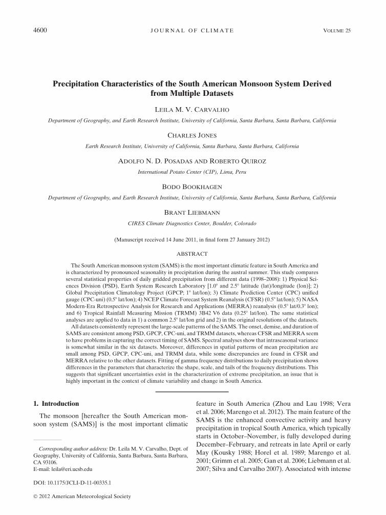
FIG. 3. First EOF patterns described as correlations between the first temporal coefficient (PC1) and precipitation anomalies. Solid(dashed) contours indicate positive (negative) correlations at 0.1 intervals (zero contours omitted). Shading indicates correlations $ 0.2(#20.2) and is significant at 5%. Data grid spacing is 2.58 lat/lon.


(GEOS) atmospheric model (Rienecker et al. 2011).Daily precipitation at 0.58 latitude/0.38 longitudeis used. As in the CFSR, precipitation is a forecastproduct.

6) Tropical Rainfall Measurement Mission (TRMM3B42 V6): the TRMM Multisatellite PrecipitationAnalysis (TMPA) (Huffman et al. 2007) providesrainfall estimates at 0.258 3 0.258 spatial resolutionand 3-h intervals. The gridded rainfall algorithm usesan optimal combination of TRMM 2B31 and TRMM2A12 data products, SSM/I, Advanced MicrowaveScanning Radiometer (AMSR), and Advanced Mi-crowave Sounding Units (AMSI) (Kummerow et al.1998; Kummerow et al. 2000). These data wereprocessed to generate daily precipitation. Previousstudies have used TRMM 3B42 V6 data to identifyrainfall-extreme events and their impact on river

discharge in the southwestern part of the Amazo-nian catchment in Bolivia and Brazil (Bookhagenand Strecker 2010). To achieve high spatial reso-lution and identify orographic rainfall processing,TRMM 2B31 data with a spatial resolution of about5 km 3 5 km and approximately daily snapshotshave been used to relate topographic characteris-tics and orographic rainfall along the eastern Andes(Bookhagen and Strecker 2008). Additional detailsof data processing are described in Bookhagen andBurbank (2011).

3. Methodology

Comparisons of precipitation variability are per-formed with several statistical methods applied to the sixdatasets regridded to a common horizontal resolution aswell as to their original grid spacings. A grid of 2.58 lat/lon spacing is selected for the same resolution compar-ison because the number of missing observations in the18 lat/lon PSD dataset is very high in some locations overSouth America (see section 4). The 2.58 lat/lon commonregrid is obtained by regridding the GPCP, CPC-uni,CFSR, MERRA, and TRMM data to the PSD grid ac-cording to the following: PR(i, j) 5 [P(i, j) 1 P(i 2 1, j) 1P(i 1 1, j) 1 P(i, j 2 1) 1 P(i, j 1 1)]/5, where PR(i, j) isthe regridded value, and the five terms on the right-handside are precipitation values from the data being trans-formed. PR(i, j) is centered on the same coordinates ofthe PSD dataset. Note that this regridding method is

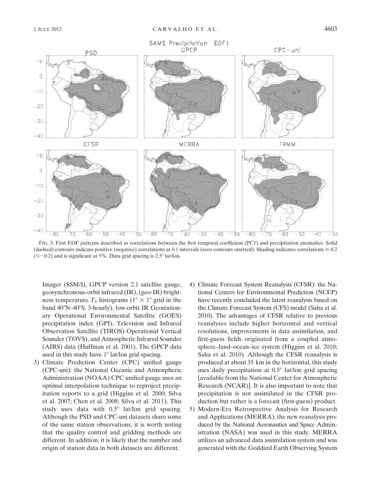
FIG. 4. (top) Mean (squares), minimum (dashes), and maximum(asterisks) dates of SAMS onset. (middle) Mean (squares), mini-mum (dashes), and maximum (asterisks) dates of SAMS demise.(bottom) Mean (squares), minimum (dashes), and maximum (as-terisks) durations of SAMS. Datasets are indicated in the hori-zontal axis. Data grid spacing is 2.58 lat/lon.

TABLE 1. Cross correlations among seasonal amplitudes ofSAMS derived from daily PC1. Correlations $ 0.63 (#20.63) aresignificant at 5%. Data grid spacing is 2.58 lat/lon.

PSD GPCP CPC-uni CFSR MERRA TRMM

PSD 1.00 — — — — —GPCP 0.85 1.00 — — — —CPC-uni 0.46 0.64 1.00 — — —CFSR 0.44 0.41 20.09 1.00 — —MERRA 0.54 0.50 20.06 0.82 — —TRMM 0.79 0.95 0.76 0.24 0.41 1.00

TABLE 2. Anomaly cross correlations among daily PC1 derivedfrom precipitation datasets. Correlations $ 0.20 (#20.20) aresignificant at 5%. Data grid spacing is 2.58 lat/lon.


PSD 1.00 — — — — —GPCP 0.67 1.00 — — — —CPC-uni 0.88 0.66 1.00 — — —CFSR 0.68 0.6 0.62 1.00 — —MERRA 0.66 0.62 0.61 0.78 1.00 —TRMM 0.75 0.9 0.74 0.63 0.64 1.00


different than the procedure used in the PSD data. ThePSD data represents gridded precipitation as averagesof precipitation over ‘‘circles’’ with radius of about 1.88;see Liebmann and Allured (2005, 2006) for details.Comparisons between both regridding methods in-dicated insignificant differences in the statisticsdescribed in section 4.

The annual evolution of SAMS is examined to de-termine consistencies and disagreements among thedatasets. The large-scale features of interest are as fol-lows: the dominant spatial precipitation pattern, dates ofonset and demise, duration, and amplitude of the mon-soon. These characteristics are determined with empir-ical orthogonal functional (EOF) analysis (Wilks 2006)applied to the daily precipitation (only land grid points)from each dataset separately. Before computation of theEOFs, the time series of precipitation in each grid pointare scaled by the square root of the cosine of the lati-tude and the long-term mean removed (1 January–31December 1998–2008). The EOFs are calculated fromcorrelation matrices. The first mode (EOF1) and associ-ated temporal coefficient (PC1) explain the largest frac-tion of the total variance of precipitation over land andare used to describe the annual evolution of SAMS.

To determine dates of onset, demise, and duration ofSAMS, the daily PC1 is smoothed with 10 passes of a

15-day moving average. This smoothing procedure isobtained empirically and is used to decrease the influenceof high-frequency variations during the transitional phasesof SAMS. The large-scale onset of SAMS is defined as thedate when the smoothed PC1 changes from negative topositive values. This implies that positive precipitationanomalies during that time become dominant over theSAMS domain. Likewise, the demise of SAMS is definedas the date when the smoothed PC1 changes from positiveto negative values. The duration of the monsoon is definedas the period between onset and demise dates. The sea-sonal amplitude of the monsoon is defined as the integralof positive unsmoothed PC1 values from onset to demise.Therefore, the seasonal amplitude index represents thesum of positive precipitation anomalies and minimizes theeffect of ‘‘break’’ periods in the monsoon especially nearthe onset and demise. Active/break periods in SAMS areparticularly frequent on intraseasonal time scales (Jonesand Carvalho 2002).

The distribution of precipitation variance is examinedwith a power spectrum of the daily PC1 during 1 October–30 April 1998–2008. The following methodology is used:1) the mean, linear trend, and annual cycle are removedfrom the PC1 time series during each season; 2) theresulting time series is tapered with a split cosine bellfunction (5% at each end); 3) fast Fourier transform

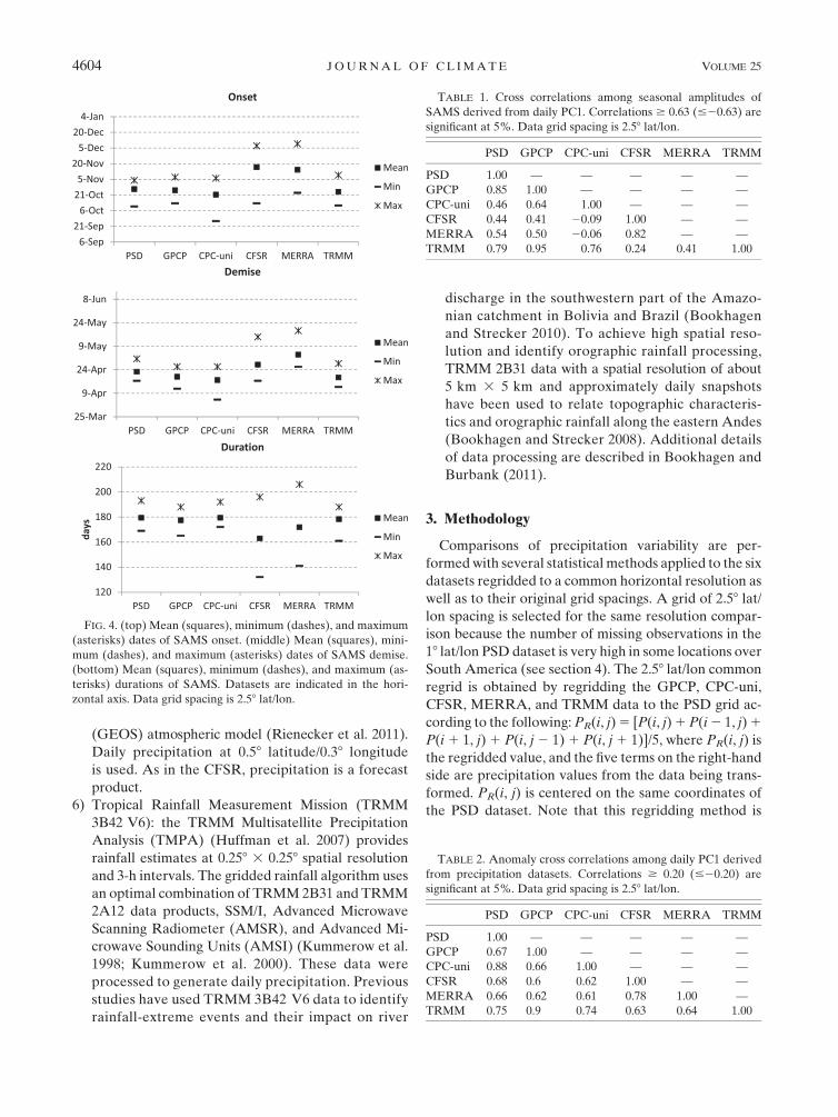
FIG. 5. Mean daily precipitation during 1 Nov–31 Mar 1979–2010. Contour interval and shading is 2 mm day21. Datasets and minimum/maximum values are indicated in each panel. Data grid spacing is 2.58 lat/lon.


(FFT) is used to obtain raw spectral estimates for eachseason; 4) the raw spectral estimates are smoothed witha running average of length L 5 3 raw spectral estimates;5) the spectra computed for each season are normalizedby the seasonal variance and averaged to obtain a 10-yrensemble mean; and 6) the degrees of freedom are es-timated initially as 60 [(2 for every raw spectral esti-mate) 3 (3 for smoothing the raw spectrum) 3 (10 forensemble average)]. The actual degrees of freedom arereduced to 52.38 because of the tapering of the timeseries [see Madden and Julian (1971) for further details].The red-noise background spectrum and 95% signifi-cance level are computed following the methodology ofMitchell (1966).

Statistical properties of precipitation are furtherstudied in the following way. Because of the skewness inprecipitation, parameters of frequency distributions areestimated and compared among the six datasets. Gammafrequency distributions are fitted to daily precipitationfollowing the maximum likelihood approach (Wilks 2006).The fitting is done on the entire sample (1 November–31March 1998–2008) of daily precipitation values Pi (zerovalues excluded). Next, the sample statistic D is computedas follows:

D 5 ln(P) 21

N!N

i51ln(Pi). (1)

Then the shape a and scale b parameters are estimatedby the polynomial approximations:

a 50:500 087 6 1 0:164 885 2D 2 0:054 427 4D2

D,

0 # D # 0:5772, (2)

a 58:898 919 1 9:059 950D 2 0:977 537 3D2

17:797 28D 1 11:968 477D2 1 D3,

0:5772 , D # 17:0, and (3)

b 5Pi

a. (4)

The gamma distribution is thus expressed as

f (P) 5(P/b)a21 exp(2P/b)

bG(a), (5)

where P, a, and b . 0, and G(a) is the gamma function.To compute the cumulative distribution function, we

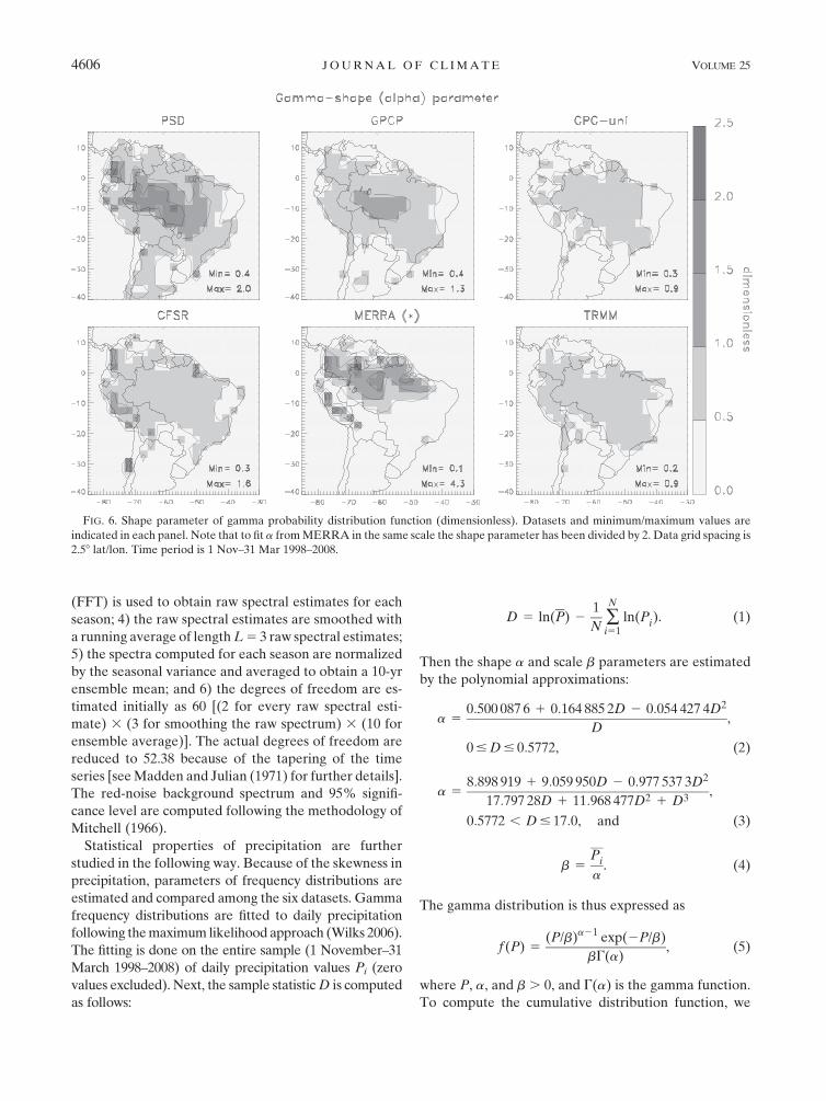
FIG. 6. Shape parameter of gamma probability distribution function (dimensionless). Datasets and minimum/maximum values areindicated in each panel. Note that to fit a from MERRA in the same scale the shape parameter has been divided by 2. Data grid spacing is2.58 lat/lon. Time period is 1 Nov–31 Mar 1998–2008.


first scale the precipitation by j 5 P/b and numericallyintegrate the incomplete gamma function F(a, j) [seeWilks (2006) for details].

Small values of the shape parameter a indicate thatthe distribution is strongly skewed to small precipitationvalues (i.e., skewed to the left), whereas large values of aindicate that the distribution tends to approximate theform of Gaussian distributions. The scale parameter brepresents the ‘‘stretch’’ or ‘‘squeeze’’ in the gammadensity function to the right or left (Wilks 2006). Exam-ples of a and b estimated over several precipitation re-gimes are discussed in Jones et al. (2004) (see their Fig. 3).

4. Comparison between PSD and CPC-uni with18 lat/lon grid spacing

It is instructive to begin by first considering the issueof precipitation sampling from surface stations in SouthAmerica. While the total number of stations shows a positivetrend over the past three decades, this aspect is in factmore complicated. Stations can be frequently deacti-vated after a few years of operation, while new stationsare brought online. The variable temporal record ofprecipitation is clearly reflected in the spatial density

of surface stations in South America (Liebmann andAllured 2005).

A comparison between PSD and CPC-uni is madesince gridded precipitation in these datasets is derivedexclusively from surface stations. The comparison isperformed at 18 lat/lon grid spacing, such that the CPC-uni data are transformed to the PSD grid. It is importantto note that PSD and CPC-uni have distinct griddingmethods. The CPC-uni is based on optimal interpolationmethod and, therefore, the quality of interpolated valuesdepends on the spatial density of stations (Chen et al.2008). The PSD is based on averaging precipitation fromstations within specified distances from grid points; if nostations are present, missing values are assigned.

Figures 1 (top, middle) respectively show the meanannual precipitation and percentage of available ob-servations in the PSD data. Grid points with fewer than70% of observations are masked. The sampling clearlyshows some geographical boundaries. For instance, ad-equate number of observations ($90%) is seen overBrazil, although it is still quite deficient over the Ama-zon. In addition, surface stations are very sparse over theAndes and northern parts of South America. Samplingbecomes even more critical in previous decades, when

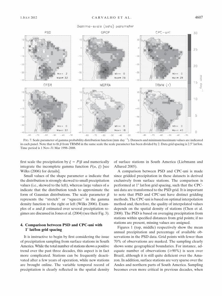
FIG. 7. Scale parameter of gamma probability distribution function (mm day21). Datasets and minimum/maximum values are indicatedin each panel. Note that to fit b from TRMM in the same scale the scale parameter has been divided by 2. Data grid spacing is 2.58 lat/lon.Time period is 1 Nov–31 Mar 1998–2008.


the density of stations over the SAMS region was low.For comparison, Fig. 1 (bottom) shows the mean annualprecipitation from CPC-uni data regridded to the same18 lat/lon of the PSD data. While the spatial patterns ofmean precipitation from both datasets are comparable,differences in intensity are noticeable especially overthe northwestern parts of South America.

A direct comparison is made by computing correla-tions between precipitation from PSD and CPC-uni ineach 18 lat/lon (Fig. 2, top). These correlations are per-formed on the raw time series (1 January–31 December1998–2008) and, therefore, include subseasonal, seasonal,and interannual variations. Because of that, one wouldexpect a high degree of agreement between the two da-tasets over the SAMS since the amplitude of the annualcycle is large. Thus, correlations are high and spatiallycoherent (above 0.8) mostly over eastern Brazil, wherethe density of stations is high (Liebmann and Allured2005). In other locations over South America, correla-tions are less spatially coherent and significantly low(correlations $ 0.2 are significant at 5%). For instance,correlations over the Amazon are on the order of 0.5–0.6.

The mean daily precipitation bias (Fig. 2, middle) is inthe range of 61.0 mm day21, which is a reasonableamount. However, the mean bias is not spatially coherent

and even changes sign among neighboring grid points. Incontrast, the root-mean-square (rms) difference (Fig. 2,bottom) is quite uniform (0.5 mm day21) over most ofBrazil and other countries. The relatively large rms dif-ference in coastal grid points in Brazil results from theregridding process since the land masks between the twodatasets do not match exactly. More importantly, rmsdifferences are consistently high ($1.0 mm day21) overa large portion of Colombia, which is surprising given thehigh number of available observations (Fig. 1, bottom).The results above highlight important differences in thegridding methods in the PSD and CPC-uni datasets.Additionally, since the number of missing data is sub-stantially high in the PSD at 18 lat/lon, further compari-sons among the datasets are performed with a commongrid of 2.58 lat/lon. This is important in the EOF analysisbecause missing data vary widely among grid points andthe calculation becomes extremely difficult with smallsample sizes.

5. Comparisons among datasets with 2.58 lat/longrid spacing

In this section, the six datasets are compared at thesame 2.58 lat/lon grid (gridded according to the description

FIG. 8. 75th percentile of daily precipitation (mm day21). Datasets and minimum/maximum values are indicated in each panel. Data gridspacing is 2.58 lat/lon. Time period is 1 Nov–31 Mar 1998–2008.


in section 3). These results can be evaluated with thecomparison at the original grid spacing resolution insection 6.

EOF analysis (section 3) is used to characterize thelarge-scale features of SAMS as represented in the dif-ferent datasets. Figure 3 shows the spatial patterns ofEOF1 derived from each dataset and expressed as cor-relations between PC1 and precipitation anomalies.Positive correlations are interpreted as positive pre-cipitation anomalies and indicative of active SAMS. Ingeneral, all datasets show similar features such as posi-tive precipitation anomalies over central South Americaand negative anomalies over the northern parts of thecontinent. The region of negative anomalies over north-ern South America is substantially smaller in the PSDbecause of missing data (the ‘‘bull’s eye’’ near 108S, 608Wis a grid point with missing data). The magnitude ofpositive correlations varies slightly and is highest forPSD. Also, the largest positive correlation in MERRA isslightest to the west relative to the other datasets. Asdiscussed in section 6, however, significant spatial dif-ferences are seen in EOF1 patterns from the datasets attheir original resolutions.

The percentages of explained variance by EOF1 arethe following: 20.5% (PSD), 11.6% (GPCP), 8.4%

(CPC-uni), 10% (CFSR), 17.9% (MERRA), and 6.9%(TRMM). EOF1 captures the largest fraction of thetotal variance, which includes subseasonal, seasonal, andinterannual variations, since the EOF analysis is per-formed removing only the long-term mean. Main dif-ferences in explained variance are associated with howmuch each PC1 represents the distribution of subseasonal,seasonal, and interannual variations. These percentagesare comparable to the percentages obtained with thedatasets at their original resolutions (section 6), whichsuggests that spatial resolution of the datasets is not themain issue but rather how each dataset represents tem-poral variations.

The seasonal variation of SAMS is represented by thedates of onset, demise, and duration. The mean onsetdate (Fig. 4, top) is highly coherent among PSD, GPCP,CPC-uni, and TRMM (;21 October) including theranges of minimum and maximum onset dates. In con-trast, the mean onset dates in the CFSR and MERRAreanalyses occur in the second week of November andthe ranges of minimum and maximum onset dates arelarger than in the other datasets. Although there is morevariability in the dates of mean demise (Fig. 4, middle),the agreement among PSD, GPCP, CPC-uni, andTRMM is relatively good. The mean demise dates in the

FIG. 9. 25th percentile of daily precipitation (mm day21). Datasets and minimum/maximum values are indicated in each panel. Data gridspacing is 2.58 lat/lon. Time period is 1 Nov–31 Mar 1998–2008.


reanalyses occur later than in the other datasets andCFSR is more consistent with the other data than MERRA.As a consequence, the mean duration of SAMS(;180 days) agrees reasonably well among PSD, GPCP,CPC-uni, and TRMM data and is shorter and more var-iable in the CFSR and MERRA (Fig. 4, bottom). Thecharacteristics shown in Fig. 4 are practically identical tosimilar results obtained from the datasets at their originalresolutions (section 6).

The seasonal amplitude (section 3) is another impor-tant characteristic of SAMS and is compared by com-puting cross correlations among the seasonal amplitudesobtained from each dataset (Table 1). Significant corre-lations are seen among PSD–GPCP (0.85), PSD–TRMM(0.79), GPCP–TRMM (0.95), CPC-uni–TRMM (0.76),and CFSR–MERRA (0.82). Surprisingly, the seasonalamplitude correlation between PSD–CPC-uni is not sta-tistically significant, even though both datasets are derivedfrom station data. Additionally, the seasonal amplitudesderived from CFSR and MERRA are correlated (al-though not statistically significant) with PSD and GPCPbut not CPC-uni. The correlations in Table 1 do not differsubstantially from similar correlations calculated from

seasonal amplitudes derived from each dataset at theiroriginal resolutions (section 6). Therefore, because ofspace limitations, the temporal variability of seasonalamplitudes (see Fig. 12) obtained from each dataset with2.58 lat/lon is not shown.

A more detailed comparison of PC1 is carried out byremoving the mean seasonal cycle in PC1 from eachdataset. Next, cross correlations are calculated among thedaily PC1 anomalies during 1 November–31 March 1998–2008 (Table 2). The best agreements are found amongGPCP–TRMM (0.90), PSD–CPC-uni (0.88), CFSR–MERRA (0.78), PSD–TRMM (0.75), and CPC-uni–TRMM (0.74), whereas the smallest correlations areamong MERRA–CPC-uni (0.61) and CFSR–GPCP (0.6).This result is important because it shows that anomalies inPC1, which are largely related to intraseasonal variations,can have different degrees of representation in the sixdatasets. Spectra of daily PC1 anomalies from datasetswith 2.58 lat/lon grid are virtually identical to spectra ofdaily PC1 anomalies from datasets with their original res-olution (section 6) and are not shown (see Fig. 13 instead).

The results above indicate that, although several as-pects of the large-scale characteristics of the SAMS are

FIG. 10. First EOF patterns described as correlations between the first temporal coefficient (PC1) and precipitation anomalies. Solid(dashed) contours indicate positive (negative) correlations at 0.1 intervals (zero contours omitted). Shading indicates correlations $ 0.2(#20.2) and is significant at 5%. Datasets have different grid spacings.


well represented in most of the datasets, some importantinconsistencies are also found. To better characterizedifferences among the datasets, the following analysesare performed on the raw precipitation (i.e., no EOF

filtering). The mean precipitation during 1 November–31 March 1998–2008 is shown in Fig. 5. The maximum isover central Amazon and the pattern extends to south-eastern Brazil in all datasets, except in MERRA wherethe maximum is clearly displaced to the north relative tothe other datasets; a pattern that is more typical of earlyspring rather than austral summer (Kousky 1988; Horelet al. 1989). The range of mean precipitation is nearlythe same in PSD, GPCP, CPC-uni, and TRMM andconsiderably high in CFSR and MERRA. In addition,the mean precipitation with 2.58 lat/lon shows sub-stantial spatial differences from the same field obtainedfrom datasets with their original resolutions especiallyover the Andes (section 6).

The distribution of precipitation can be evaluatedwith the parameters of the Gamma frequency distribu-tion. The shape parameter (Fig. 6) is in the range 0.5–1.0over most of South America (except the Andes) andindicates the skewness of precipitation to small values.This feature is consistent in the PSD, GPCP, CPC-uni,CFSR, and TRMM data, whereas PSD and GPCP datashow values larger than 1.0 over the core of the monsoon.It is also worth noting that, while PSD and CPC-uni arebased on station data, the precipitation distribution overthe core of the monsoon can be very different in thesedatasets. Another obvious feature is that a obtained fromMERRA has a spatial pattern and magnitudes substan-tially different than any other dataset.

The scale parameter b (Fig. 7) from all datasetsconsistently shows large values ($10) over southernSouth America with maximum centered over northern

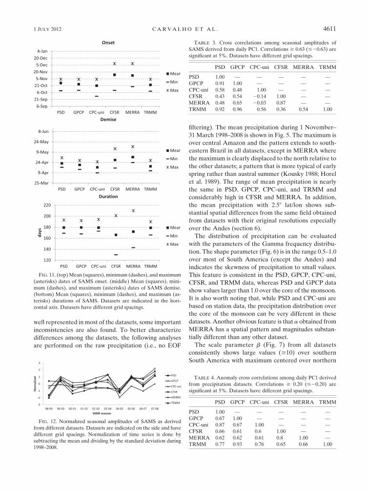
FIG. 11. (top) Mean (squares), minimum (dashes), and maximum(asterisks) dates of SAMS onset. (middle) Mean (squares), mini-mum (dashes), and maximum (asterisks) dates of SAMS demise.(bottom) Mean (squares), minimum (dashes), and maximum (as-terisks) durations of SAMS. Datasets are indicated in the hori-zontal axis. Datasets have different grid spacings.

FIG. 12. Normalized seasonal amplitudes of SAMS as derivedfrom different datasets. Datasets are indicated on the side and havedifferent grid spacings. Normalization of time series is done bysubtracting the mean and dividing by the standard deviation during1998–2008.

TABLE 3. Cross correlations among seasonal amplitudes ofSAMS derived from daily PC1. Correlations $ 0.63 (#20.63) aresignificant at 5%. Datasets have different grid spacings.


PSD 1.00 — — — — —GPCP 0.91 1.00 — — — —CPC-uni 0.58 0.48 1.00 — — —CFSR 0.43 0.54 20.14 1.00 — —MERRA 0.48 0.65 20.03 0.87 — —TRMM 0.92 0.96 0.56 0.36 0.54 1.00

TABLE 4. Anomaly cross correlations among daily PC1 derivedfrom precipitation datasets. Correlations $ 0.20 (#20.20) aresignificant at 5%. Datasets have different grid spacings.


PSD 1.00 — — — — —GPCP 0.67 1.00 — — — —CPC-uni 0.87 0.67 1.00 — — —CFSR 0.66 0.61 0.6 1.00 — —MERRA 0.62 0.62 0.61 0.8 1.00 —TRMM 0.77 0.93 0.76 0.65 0.66 1.00


Argentina. The spatial pattern of b shows some similar-ities between PSD and CPC-uni over tropical SouthAmerica, although the magnitudes are different. Differ-ent spatial patterns and magnitudes are seen in GPCPand CFSR over the core of the monsoon. While the bspatial pattern from TRMM is consistent with PSD andCPC-uni over the SAMS, the magnitudes are excessively

large. It is interesting to note that b from MERRA issignificantly different than any other dataset over thenorthern Amazon.

Further insight about the distribution of precipitationis noted on the 75th percentile (P75) (Fig. 8). It is en-couraging that the northwest–southeast orientation andthe range of magnitudes of P75 from PSD and CPC-uni

FIG. 13. Power spectrum of PC1. Smoothed (dashed) lines indicate the background red-noise spectrum (95%confidence level). Datasets have different grid spacings. Spectra were computed from daily PC1 during 1 Oct–30 Apr1998–2008.


agree over the SAMS. TRMM and GPCP P75 showsimilar range of magnitudes over SAMS, although TRMMindicates large values where the Amazon River meets theAtlantic Ocean. P75 from CFSR also shows a northwest–southeast orientation as in PSD and CPC-uni, while largevalues are found over the Amazon. In contrast, MERRAshows P75 $ 10 mm day21 displaced over northernAmazon clearly indicative of difficulties in properly rep-resenting the precipitation pattern over the core of themonsoon.

The 25th percentile (P25) (Fig. 9) is less than2 mm day21 over large portions of South America inall datasets. Over the core of the monsoon, PSD, GPCP,CPC-uni, CFSR, and TRMM indicate P25 in the rangeof 2.0–4.0 mm day21, although the spatial extent variesamong these datasets. As before, P25 derived fromMERRA shows values larger than 2.0 mm day21 dis-placed over the northern Amazon.

6. Comparisons among datasets with originalresolutions

The same type of analysis is performed for the data-sets with their original resolution: PSD (2.58 lat/lon),

GPCP (1.08 lat/lon), CPC-uni (0.58 lat/lon), CFSR (0.58lat/lon), MERRA (0.58 lat/0.38 lon), and TRMM (0.258lat/lon). Figure 10 shows the spatial patterns of EOF1.As expected, the higher the spatial resolution, the moredetails are represented in the horizontal, although somefeatures are obviously suspicious, for example, over thecentral Andes. Some of these can be explained by a lackof precipitation gauges or abnormal land cover conditionsthat influence satellite-derived precipitation values. Alldatasets consistently indicate a region of positive pre-cipitation anomalies over the core of the monsoon regionand negative anomalies over northern South America.Moreover, although positive precipitation anomalies overthe central Andes are consistently represented in theGPCP, CPC-uni, CFSR, MERRA, and TRMM, the largegradients in correlations shown in CFSR and MERRAsuggest that the reanalysis products overestimate precip-itation in that region.

The percentages of total variance explained by EOF1are the following: 20.5% (PSD), 9.7% (GPCP), 7.6%(CPC-uni), 8.9% (CFSR), 17.5% (MERRA), and 7.3%(TRMM), respectively. The distribution of percentagesare comparable to the percentages obtained with alldatasets with the same resolution (section 5), whichsuggests that the spatial resolution is not the main factor

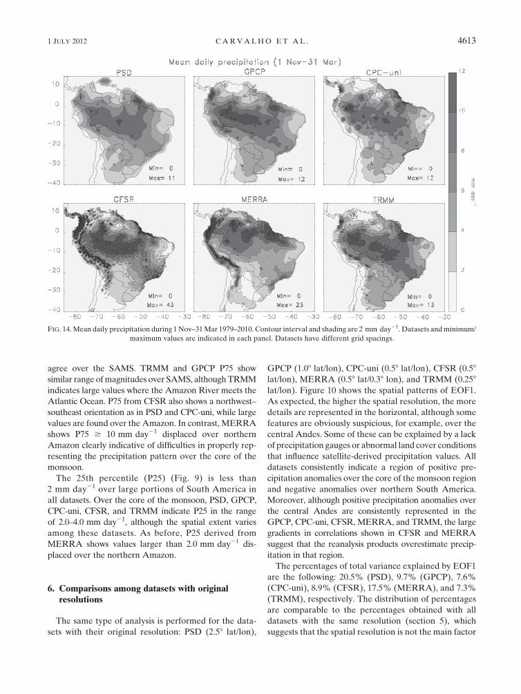
FIG. 14. Mean daily precipitation during 1 Nov–31 Mar 1979–2010. Contour interval and shading are 2 mm day21. Datasets and minimum/maximum values are indicated in each panel. Datasets have different grid spacings.


in explaining these differences. The temporal variabilityof PC1, especially the distribution of intraseasonal var-iance (see power spectra next), may explain some ofthese differences.

Dates of onset, demise, and duration of SAMS areshown in Fig. 11 and can be compared with the samedata resolution results (Fig. 4). Identical patterns arenoted such that the mean onset date (Fig. 11, top) ishighly coherent among PSD, GPCP, CPC-uni, andTRMM (;21 October) including the ranges of mini-mum and maximum onset dates. In contrast, the meanonset dates in CFSR and MERRA are off by severalweeks. The variability in dates of mean demise (Fig. 11,middle) indicates agreements among PSD, GPCP,CPC-uni, and TRMM and some differences in CFSRand large disagreement in MERRA. Consequently, themean durations of SAMS (;180 days) agree reasonablywell among PSD, GPCP, CPC-uni, and TRMM data andis shorter and more variable in the CFSR and MERRAreanalyses (Fig. 11, bottom). These results indicate thatdifferences in data resolution do not explain disagree-ments in the annual evolution of SAMS especially be-tween CFSR and MERRA and the other datasets.

Fig. 12 shows the temporal variability of the seasonalamplitude of SAMS in each dataset. Since the magnitudes

of PC1 vary significantly among the datasets, the ampli-tudes are normalized by removing the mean seasonalamplitude and dividing by the standard deviation ofthe 10 seasons (1998–2008). This allows visualizing theseasonal amplitudes on the same scale. Table 3 showsthe cross correlations in seasonal amplitudes and canbe compared with Table 1. The largest differencesrelative to the same resolution correlations are be-tween PSD–TRMM (0.92), CPC-uni–GPCP (0.48),GPCP–CFSR (0.54), GPCP–MERRA (0.65), CPC-uni–TRMM (0.56), and MERRA–TRMM (0.54). Thecorrelations between reanalyses and CPC-uni are sur-prisingly negative (20.03, 20.14). It is interesting to notethat all datasets consistently indicate a short-term trendin seasonal amplitudes of SAMS after 2004, which agreeswith L. M. V. Carvalho et al. (2011, unpublished manu-script), who investigated long-term changes in SAMSlarge-scale circulation and warming in South Americaand Atlantic Ocean.

As before, the mean annual cycle is removed from thePC1 series and cross correlations among the datasets arecomputed (Table 4). A comparison between these re-sults and Table 2 shows only very minor differences. Thisindicates that differences in the representation of sub-seasonal and interannual variations among the datasets

FIG. 15. Shape parameter of gamma probability distribution function (dimensionless). Datasets and minimum/maximum values areindicated in each panel. Note that to fit a from MERRA in the same scale the shape parameter has been divided by 2. Datasets havedifferent grid spacings. Time period is 1 Nov–31 Mar 1998–2008.


do not vary significantly with spatial resolution. Evidently,these conclusions hold for the large-scale aspects ofSAMS inferred from one EOF mode. Locally, differencesin subseasonal, seasonal, and interannual variations canvary significant among the datasets and spatial resolutionscan be important.

Several studies have shown that intraseasonal variationsplay an important role in modulating the variability ofSAMS (Nogues-Paegle and Mo 1997; Liebmann et al.1999; Nogues-Paegle et al. 2000; Jones and Carvalho 2002;Cunningham and Cavalcanti 2006; Gonzalez et al. 2008;Muza et al. 2009; Carvalho et al. 2011b). When calculatedfrom outgoing longwave radiation (OLR) anomalies, thefirst EOF shows regions of positive and negative anoma-lies associated with the eastward propagation of the MJOas well as midlatitude wave trains propagating over east-ern South America.

The spectra from daily PC1 (Fig. 13) indicate thatintraseasonal variations (;20–90 days) are captured byall datasets, although with different degrees of ampli-tude. Most noticeably, the intraseasonal spectral peakfrom GPCP exceeds the 95% confidence level above thebackground red noise. Similar peaks are evident in CPC-uni, MERRA, and TRMM, although they barely exceedthe 95% significance level. It should be noted that the

spectra derived from 2.58 lat/lon data are identical to theresults in Fig. 13 indicating that the large-scale repre-sentation of subseasonal variations vary among the da-tasets but spatial resolution is not the dominant factor.

Fig. 14 shows the mean precipitation during 1November–31 March 1998–2008 and can be comparedwith Fig. 5. In general, differences in spatial patternsof mean precipitation are small among PSD, GPCP,CPC-uni, and TRMM data. These datasets consistentlyshow maximum precipitation over the central Amazonincluding the extensions to southeastern Brazil and to-ward Amapa state, where the Amazon River meets theAtlantic Ocean. The mean precipitation in the PSD datais slightly less than in GPCP, CPC-uni, and TRMM data(minimum and maximum values are indicated in eachpanel). It is also interesting to note that GPCP, CPC-uni,and TRMM data agree in the high precipitation overColombia, whereas the agreement is less obvious overPeru. Although precipitation from the new reanalysescertainly improves from previous reanalyses (Bosilovichet al. 2008; Rienecker et al. 2011; Silva et al. 2011),substantial discrepancies are observed in the CFSR andMERRA reanalyses relative to the other datasets.While the spatial pattern of mean CFSR precipitationover the central Amazon is somewhat consistent with

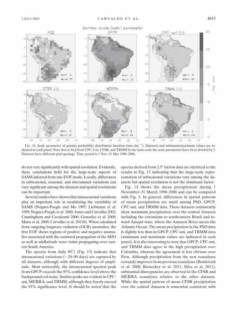
FIG. 16. Scale parameter of gamma probability distribution function (mm day21). Datasets and minimum/maximum values are in-dicated in each panel. Note that to fit b from CPC-Uni, CFSR, and TRMM in the same scale the scale parameters have been divided by 2.Datasets have different grid spacings. Time period is 1 Nov–31 Mar 1998–2008.


the other datasets (except MERRA), CFSR precipita-tion is unrealistically large and spotty over the Andesand southeastern Brazil and the maximum precipitation(43 mm day21) is significantly larger than in the PSD,GPCP, CPC-uni, and TRMM data. These features aremuch less evident in the 2.58 lat/lon comparison (Fig. 5).The spatial pattern of mean precipitation in MERRAappears shifted to the north relative to the other datasets.Although the MERRA precipitation is not as spotty asthe CFSR data in some locations, precipitation is exces-sive over the Andes Mountains and the maximum pre-cipitation (23 mm day21) is higher than in PSD, GPCP,CPC-uni, and TRMM data.

The shape parameter (Fig. 15) is quite comparable with2.58 lat/lon data (Fig. 6), although some differences areworth noting. For instance, the region of a $ 1.0 over theAmazon obtained with 2.58 lat/lon GPCP data (Fig. 6) ispractically absent in the 18 lat/lon comparison (Fig. 15).This suggests that spatially averaging precipitation in-creases a and, therefore, might explain a $ 1.0 over theAmazon obtained from PSD data. Except for small spa-tial variations, 0.5 # a # 1.0 over a large area over SouthAmerica as derived from GPCP, CPC-uni, CFSR, andTRMM. The shape parameter estimated from MERRAreanalysis is markedly different than any other dataset

both in spatial pattern and magnitudes (i.e., the field wasdivided by 2 to fit the same scale).

The patterns of scale parameter (Fig. 16) obtainedfrom datasets at their original resolution are somewhatsimilar to the b derived with 2.58 lat/lon grids (Fig. 7).Note, however, that the range of values increase in somedatasets (CPC-uni, CFSR, and TRMM), and b has beendivided by 2 to fit in the same scale as the other datasets.Values b $ 10 are seen over southern South Americawith maximum centered over northern Argentina. Thespatial patterns of b between PSD and CPC-uni aresimilar over tropical South America, although themagnitudes are twice as large in CPC-uni. The b spatialpattern from TRMM is consistent with PSD, althoughthe magnitudes are much larger in the former. MERRAis significantly different than any other dataset over thenorthern Amazon.

To further characterize the frequency distributions ofprecipitation, Fig. 17 shows the 75th percentile (P75)and can be compared with Fig. 8. The spatial pattern ofP75 is quite similar between PSD and CPC-uni and, tosome extent, between GPCP and TRMM, although themagnitudes vary among these datasets. While the spatialpattern of P75 from CFSR is similar to the GPCP–TRMMpatterns, the magnitudes are very different. Interestingly,

FIG. 17. 75th percentile of daily precipitation (mm day21). Datasets and minimum/maximum values are indicated in each panel. Notethat to fit the 75th percentile from CFSR in the same scale the percentile has been divided by 2. Datasets have different grid spacings. Timeperiod is 1 Nov–31 Mar 1998–2008.


MERRA shows P75 comparable to PSD, GPCP, andCPC-uni over central–southeastern Brazil, but the pat-ter is different over the northern Amazon.

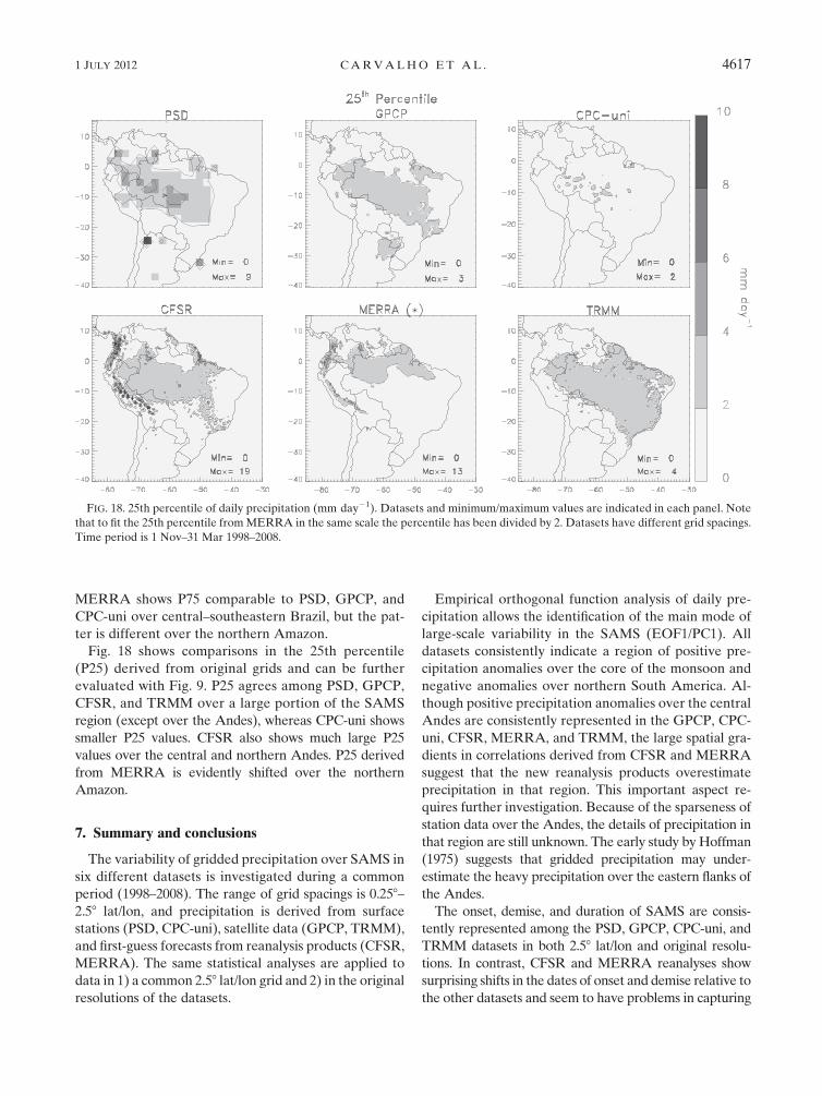
Fig. 18 shows comparisons in the 25th percentile(P25) derived from original grids and can be furtherevaluated with Fig. 9. P25 agrees among PSD, GPCP,CFSR, and TRMM over a large portion of the SAMSregion (except over the Andes), whereas CPC-uni showssmaller P25 values. CFSR also shows much large P25values over the central and northern Andes. P25 derivedfrom MERRA is evidently shifted over the northernAmazon.

7. Summary and conclusions

The variability of gridded precipitation over SAMS insix different datasets is investigated during a commonperiod (1998–2008). The range of grid spacings is 0.258–2.58 lat/lon, and precipitation is derived from surfacestations (PSD, CPC-uni), satellite data (GPCP, TRMM),and first-guess forecasts from reanalysis products (CFSR,MERRA). The same statistical analyses are applied todata in 1) a common 2.58 lat/lon grid and 2) in the originalresolutions of the datasets.

Empirical orthogonal function analysis of daily pre-cipitation allows the identification of the main mode oflarge-scale variability in the SAMS (EOF1/PC1). Alldatasets consistently indicate a region of positive pre-cipitation anomalies over the core of the monsoon andnegative anomalies over northern South America. Al-though positive precipitation anomalies over the centralAndes are consistently represented in the GPCP, CPC-uni, CFSR, MERRA, and TRMM, the large spatial gra-dients in correlations derived from CFSR and MERRAsuggest that the new reanalysis products overestimateprecipitation in that region. This important aspect re-quires further investigation. Because of the sparseness ofstation data over the Andes, the details of precipitation inthat region are still unknown. The early study by Hoffman(1975) suggests that gridded precipitation may under-estimate the heavy precipitation over the eastern flanks ofthe Andes.

The onset, demise, and duration of SAMS are consis-tently represented among the PSD, GPCP, CPC-uni, andTRMM datasets in both 2.58 lat/lon and original resolu-tions. In contrast, CFSR and MERRA reanalyses showsurprising shifts in the dates of onset and demise relative tothe other datasets and seem to have problems in capturing

FIG. 18. 25th percentile of daily precipitation (mm day21). Datasets and minimum/maximum values are indicated in each panel. Notethat to fit the 25th percentile from MERRA in the same scale the percentile has been divided by 2. Datasets have different grid spacings.Time period is 1 Nov–31 Mar 1998–2008.


the correct timing of SAMS. The spectral variance inprecipitation is examined by computing power spectra ofdaily PC1 time series. It is encouraging that the distributionof intraseasonal variance is somewhat similar in bothcomparisons (2.58 lat/lon and original grids), indicating thatthe large-scale representation of subseasonal variationsagree among the datasets. Because of the limited datasampling (10 yr), differences in interannual variabilityamong the datasets are not explored here.

Comparisons of mean precipitation during the monsoonindicate that differences in spatial patterns are smallamong PSD, GPCP, CPC-uni, and TRMM data and somediscrepancies are found in the CFSR and MERRA rean-alyses. While the spatial pattern of mean CFSR precip-itation over the central Amazon is somewhat consistentwith the other datasets (except MERRA), CFSR precip-itation is unrealistically large and spotty over the Andesand southeastern Brazil and the maximum precipitation(43 mm day21 with 0.58 lat/lon) is significantly larger thanin the PSD, GPCP, CPC-uni, and TRMM data. Theseresults appear consistent with Silva et al. (2011), who com-pared CFSR against the NCEP–NCAR (R1) and NCEP–Department of Energy (DOE) (R2) reanalyses and theCPC-uni precipitation. They noted that, although precip-itation from CFSR is more consistent with observationsthan R1 and R2, large biases are still present, particularlyduring the SAMS when CFSR appears to overestimateprecipitation. Moreover, Silva et al. (2011) showed thatCFSR has substantial biases in intensity and frequency ofprecipitation events. One of the most worrisome findingsis that the spatial pattern of mean precipitation fromMERRA appears shifted to the north relative to the otherdatasets, which is not typical of the summer monsoon.

Last, the results of this study highlight an importantissue that has yet to be resolved before reliable assess-ments of climate changes in South America can beachieved. The fitting of gamma frequency distributionsto daily precipitation shows significant differencesamong all datasets in the parameters that characterizethe shape, scale, and tails of the distributions. This im-plies that significant uncertainties exist in the charac-terization of extreme precipitation in these datasets.These discrepancies are not only relevant over theAmazon, where the maximum climatological precip-itation amount is observed, but are also remarkable overthe eastern Andes and east-central Brazil. These regionsare highly susceptible to long-term changes in SAMScharacteristics (L. M. V. Carvalho et al. 2011, unpublishedmanuscript; Carvalho et al. 2011a).

Acknowledgments. L. M. V. Carvalho, C. Jones, andB. Liebmann thank the support of NOAA’s Climate Pro-gram Office (NA07OAR4310211 and NA10OAR4310170).

L. M. V Carvalho, C. Jones, A. Posadas, and R. Quirozthank USAID-CIP (Subcontract SB100085). L. M. VCarvalho and C. Jones thank the NSF Rapid Program(AGS-1126804). NCEP–NCAR reanalysis and OLRdata were provided by the NOAA/OAR/ESRL PSD,Boulder, Colorado (www.esrl.noaa.gov). TRMM datawere acquired by an international joint project spon-sored by the Japan National Space DevelopmentAgency (NASDA) and the U.S. National AeronauticsSpace Administration (NASA) Office of Earth Science.The help from Bob Dattore, NCAR-CISL, in providingthe NCEP CFSR data is greatly appreciated.

REFERENCES

Berbery, E. H., and E. A. Collini, 2000: Springtime precipitationand water vapor flux over southeastern South America. Mon.Wea. Rev., 128, 1328–1346.

Bookhagen, B., and M. R. Strecker, 2008: Orographic barriers,high-resolution TRMM rainfall, and relief variations along theeastern Andes. Geophys. Res. Lett., 35, L06403, doi:10.1029/2007GL032011.

——, and ——, 2010: Modern Andean rainfall variation duringENSO cycles and its impact on the Amazon basin. NeogeneHistory of Western Amazonia and Its Significance for ModernDiversity, C. Hoorn, H. Vonhof, and F. Wesselingh, Eds.,Blackwell Publishing, 223–41.

——, and D. W. Burbank, 2011: Towards a complete Himalayanhydrologic budget: The spatiotemporal distribution of snowmelt and rainfall and their impact on river discharge. J. Geo-phys. Res., 115, F03019, doi:10.1029/2009JF001426.

Bosilovich, M. G., J. Chen, F. R. Robertson, and R. F. Adler, 2008:Evaluation of global precipitation in reanalyses. J. Appl. Me-teor. Climatol., 47, 2279–2299.

Carvalho, L. M. V., C. Jones, and B. Liebmann, 2002a: Extremeprecipitation events in southeastern South America and large-scale convective patterns in the South Atlantic convergencezone. J. Climate, 15, 2377–2394.

——, ——, and M. A. F. Silva Dias, 2002b: Intraseasonal large-scale circulations and mesoscale convective activity in tropicalSouth America during the TRMM-LBA campaign. J. Geo-phys. Res., 107, 8042, doi:10.1029/2001JD000745.

——, ——, and B. Liebmann, 2004: The South Atlantic conver-gence zone: Intensity, form, persistence, and relationshipswith intraseasonal to interannual activity and extreme rainfall.J. Climate, 17, 88–108.

——, ——, A. E. Silva, B. Liebmann, and P. L. S. Dias, 2011a:The South American monsoon system and the 1970s climatetransition. Int. J. Climatol., 31, 1248–1256, doi:10.1002/joc.2147.

——, A. E. Silva, C. Jones, B. Liebmann, and H. Rocha, 2011b:Moisture transport and intraseasonal variability in the SouthAmerica monsoon system. Climate Dyn., 36, 1865–1880.

Chen, M. Y., W. Shi, P. P. Xie, V. B. S. Silva, V. E. Kousky, R. W.Higgins, and J. E. Janowiak, 2008: Assessing objective tech-niques for gauge-based analyses of global daily precipitation.J. Geophys. Res., 113, D04110, doi:10.1029/2007JD009132.

Cunningham, C. A. C., and I. F. D. Cavalcanti, 2006: Intraseasonalmodes of variability affecting the South Atlantic convergencezone. Int. J. Climatol., 26, 1165–1180.


Dee, D. P., and Coauthors, 2011: The ERA-Interim reanalysis:Configuration and performance of the data assimilation system.Quart. J. Roy. Meteor. Soc., 137, 553–597, doi:10.1002/qj.828.

Durieux, L., L. A. T. Machado, and H. Laurent, 2003: The impactof deforestation on cloud cover over the Amazon arc of de-forestation. Remote Sens. Environ., 86, 132–140.

Gan, M. A., V. B. Rao, and M. C. L. Moscati, 2006: South Amer-ican monsoon indices. Atmos. Sci. Lett., 6, 219–223.

Gandu, A. W., and P. L. Silva Dias, 1998: Impact of tropical heatsources on the South American tropospheric upper circulationand subsidence. J. Geophys. Res., 103 (D6), 6001–6015.

Gonzalez, P. L. M., C. S. Vera, B. Liebmann, and G. Kiladis, 2008:Intraseasonal variability in subtropical South America as de-picted by precipitation data. Climate Dyn., 30, 727–744.

Grimm, A. M., 2003: The El Nino impact on the summer monsoonin Brazil: Regional processes versus remote influences.J. Climate, 16, 263–280.

——, 2004: How do La Nina events disturb the summer monsoonsystem in Brazil? Climate Dyn., 22, 123–138.

——, and M. T. Zilli, 2009: Interannual variability and seasonalevolution of summer monsoon rainfall in South America.J. Climate, 22, 2257–2275.

——, C. S. Vera, and C. R. Mechoso, 2005: The South Americanmonsoon system. The American Monsoon Systems: An In-troduction, C.-P. Chang, B. Wang, and N.-C. G. Lau, Eds.,World Meteorological Organization, 197–206.

Hartmann, D. L., and E. E. Recker, 1986: Diurnal variation ofoutgoing longwave radiation in the tropics. J. Climate Appl.Meteor., 25, 800–812.

Higgins, R. W., W. Shi, E. Yarosh, and R. Joyce, 2000: ImprovedUnited States precipitation quality control system and analy-sis. NCEP/Climate Prediction Center Atlas 7, 40 pp.

——, V. E. Kousky, V. B. S. Silva, E. Becker, and P. Xie, 2010:Intercomparison of daily precipitation statistics over theUnited States in observations and in NCEP reanalysis prod-ucts. J. Climate, 23, 4637–4650.

Hoffman, J., 1975: Maps of mean temperature and precipitation.Climatic Atlas of South America, Vol. 1, World Meteorologi-cal Organization, 1–28.

Horel, J. D., A. N. Hahmann, and J. E. Geisler, 1989: An in-vestigation of the annual cycle of convective activity over thetropical Americas. J. Climate, 2, 1388–1403.

Huffman, G. J., and Coauthors, 2001: Global precipitation at one-degree daily resolution from multisatellite observations.J. Hydrometeor., 2, 36–50.

——, and Coauthors, 2007: The TRMM Multisatellite PrecipitationAnalysis (TMPA): Quasi-global, multiyear, combined-sensorprecipitation estimates at fine scales. J. Hydrometeor., 8,38–55.

Jones, C., and L. M. V. Carvalho, 2002: Active and break phases inthe South American monsoon system. J. Climate, 15, 905–914.

——, D. E. Waliser, K. M. Lau, and W. Stern, 2004: Global occur-rences of extreme precipitation and the Madden–Julian oscilla-tion: Observations and predictability. J. Climate, 17, 4575–4589.

Kodama, Y. M., 1992: Large-scale common features of subtropicalprecipitation zones (the baiu frontal zone, the SPCZ, and theSACZ). 1. Characteristics of subtropical frontal zones.J. Meteor. Soc. Japan, 70, 813–836.

——, 1993: Large-scale common features of subtropical conver-gence zones (the baiu frontal zone, the SPCZ, and the SACZ).2. Conditions of the circulations for generating the STCZs.J. Meteor. Soc. Japan, 71, 581–610.

Kousky, V. E., 1988: Pentad outgoing longwave radiation climatologyfor the South American sector. Rev. Bras. Meteor., 3, 217–231.

Kummerow, C., W. Barnes, T. Kozu, J. Shiue, and J. Simpson, 1998:The Tropical Rainfall Measuring Mission (TRMM) sensorpackage. J. Atmos. Oceanic Technol., 15, 809–817.

——, and Coauthors, 2000: The status of the Tropical RainfallMeasuring Mission (TRMM) after two years in orbit. J. Appl.Meteor., 39, 1965–1982.

Legates, D. R., and C. J. Willmott, 1990: Mean seasonal and spa-tial variability in gauge-corrected, global precipitation. Int.J. Climatol., 10, 111–127.

Lenters, J. D., and K. H. Cook, 1999: Summertime precipitationvariability over South America: Role of the large-scale cir-culation. Mon. Wea. Rev., 127, 409–431.

Liebmann, B., and D. Allured, 2005: Daily precipitation grids forSouth America. Bull. Amer. Meteor. Soc., 86, 1567–1570.

——, and ——, 2006: Reply. Bull. Amer. Meteor. Soc., 87, 1096–1096.

——, G. N. Kiladis, J. A. Marengo, T. Ambrizzi, and J. D. Glick, 1999:Submonthly convective variability over South America and theSouth Atlantic convergence zone. J. Climate, 12, 1877–1891.

——, C. Jones, and L. M. V. Carvalho, 2001: Interannual variabilityof daily extreme precipitation events in the state of Sao Paulo,Brazil. J. Climate, 14, 208–218.

——, G. N. Kiladis, C. S. Vera, A. C. Saulo, and L. M. V. Carvalho,2004: Subseasonal variations of rainfall in South America inthe vicinity of the low-level jet east of the Andes and com-parison to those in the South Atlantic convergence zone.J. Climate, 17, 3829–3842.

——, and Coauthors, 2007: Onset and end of the rainy season inSouth America in observations and the ECHAM 4.5 atmo-spheric general circulation model. J. Climate, 20, 2037–2050.

Madden, R. A., and P. R. Julian, 1971: Detection of a 40–50 dayoscillation in the zonal wind in the tropical Pacific. J. Atmos.Sci., 28, 702–708.

Marengo, J. A., 2004: Interdecadal variability and trends of rainfallacross the Amazon basin. Theor. Appl. Climatol., 78, 79–96.

——, 2009: Long-term trends and cycles in the hydrometeorology of theAmazon basin since the late 1920s. Hydrol. Proc., 23, 3236–3244.

——, B. Liebmann, V. E. Kousky, N. P. Filizola, and I. C. Wainer,2001: Onset and end of the rainy season in the BrazilianAmazon basin. J. Climate, 14, 833–852.

——, M. W. Douglas, and P. L. S. Dias, 2002: The South Americanlow-level jet east of the Andes during the 1999 LBA-TRMMand LBA-WET AMC campaign. J. Geophys. Res., 107, 8079,doi:10.1029/2001JD001188.

——, and Coauthors, 2012: Recent developments on the SouthAmerican monsoon system. Int. J. Climatol., 32, 1–21, doi:10.1002/joc.2254.

Mitchell, J. M., Jr, 1966: Climate change. World MeteorologicalOrganization Tech. Note 79, 79 pp. [Available from WMO, 41Avenue Giuseppe-Motta-1211, Geneva 2, Switzerland.]

Muza, M. N., L. M. V. Carvalho, C. Jones, and B. Liebmann, 2009:Intraseasonal and interannual variability of extreme dry andwet events over southeastern South America and subtropicalAtlantic during the austral summer. J. Climate, 22, 1682–1699.

Nogues-Paegle, J., and K. C. Mo, 1997: Alternating wet and dryconditions over South America during summer. Mon. Wea.Rev., 125, 279–291.

——, L. A. Byerle, and K. C. Mo, 2000: Intraseasonal modulation ofSouth American summer precipitation. Mon. Wea. Rev., 128,837–850.


Rienecker, M. M., and Coauthors, 2011: MERRA—NASA’sModern-Era Retrospective Analysis for Research and Ap-plications. J. Climate, 24, 3624–3648.

Robertson, A. W., and C. R. Mechoso, 1998: Interannual and de-cadal cycles in river flows of southeastern South America.J. Climate, 11, 2570–2581.

——, and ——, 2000: Interannual and interdecadal variability of theSouth Atlantic convergence zone. Mon. Wea. Rev., 128, 2947–2957.

Saha, S., and Coauthors, 2010: The NCEP Climate Forecast SystemReanalysis. Bull. Amer. Meteor. Soc., 91, 1015–1057.

Silva, A. E., and L. M. V. Carvalho, 2007: Large-scale index forSouth America monsoon (LISAM). Atmos. Sci. Lett., 8, 51–57.

Silva, V. B. S., V. E. Kousky, W. Shi, and R. W. Higgins, 2007: Animproved gridded historical daily precipitation analysis forBrazil. J. Hydrometeor., 8, 847–861.

——, ——, and R. W. Higgins, 2011: Daily precipitation statis-tics for South America: An intercomparison between NCEPreanalyses and observations. J. Hydrometeor., 12, 101–117.

Silva Dias, P. L., W. H. Schubert, and M. DeMaria, 1983: Large-scale response of the tropical atmosphere to transient con-vection. J. Atmos. Sci., 40, 2689–2707.

Vera, C., and Coauthors, 2006: Toward a unified view of theAmerican monsoon systems. J. Climate, 19, 4977–5000.

Wilks, D. S., 2006: Statistical Methods in the Atmospheric Sciences.2nd ed. Vol. 91, Academic Press, 648 pp.

Xie, P. P., and Coauthors, 2003: GPCP pentad precipitationanalyses: An experimental dataset based on gauge observa-tions and satellite estimates. J. Climate, 16, 2197–2214.

Zhou, J. Y., and K. M. Lau, 1998: Does a monsoon climate existover South America? J. Climate, 11, 1020–1040.


Precipitation Characteristics of the South American...

Documents

Transcript of Precipitation Characteristics of the South American...