Praise for Effective SQL

“Given the reputation of the authors, I expected to be impressed. Impressed doesn’t cover it, though. I was blown away! Most SQL books tell you ‘how.’ This one tells you ‘why.’ Most SQL books separate database design from implementa-tion. This one integrates design considerations into every facet of SQL use. Most SQL books sit on my shelf. This one will live on my desk.”

—Roger Carlson, Microsoft Access MVP (2006–2015)

“It can be easy to learn the basics of SQL, but it is very difficult to build accurate and efficient SQL, especially for critical systems with complex requirements. But now, with this great new book, you can get up to speed and write effective SQL much more quickly, no matter which DBMS you use.”

— Craig S. Mullins, Mullins Consulting, Inc., DB2 Gold Consultant and IBM Cham-pion for Analytics

“This is a great book. It is written in language that can be understood by a rela-tive beginner and yet contains tips and tricks that will benefit the most hardened workhorse. It will therefore appeal to readers across the whole range of expertise and should be in the library of anybody who is seriously concerned with design-ing, managing, or programming databases.”

—Graham Mandeno, database consultant and Microsoft MVP (1996–2015)

“This book is an excellent resource for database designers and developers working with relational and SQL-based databases—it’s an easy read with great examples that combine theory with practical examples seamlessly. Examples for top rela-tional databases Oracle, DB2, SQL Server, MySQL, and PostgreSQL are included throughout. The book walks the reader through sophisticated techniques to deal with things such as hierarchical data and tally tables, along with explanations of the inner workings and performance implications of SQL using GROUP BY, EXISTS, IN, correlated and non-correlated subqueries, window functions, and joins. The tips you won’t find anywhere else, and the fun examples help to make this book stand out from the crowd.”

—Tim Quinlan, database architect and Oracle Certified DBA

“This book is good for those who need to support multiple dialects of SQL. It’s divided up into stand-alone items that you just grab and go. I have been doing SQL in various flavors since 1992 and even I picked up a few things.”

—Tom Moreau, Ph.D., SQL Server MVP (2001–2012)

“This book is a powerful, compact, and easily understandable presentation of how to use SQL—it shows the application of SQL to real-world questions in order to teach the construction of queries, and it explains the relationship of ‘how data is stored’ to ‘how data is queried’ so that you obtain results successfully and effectively.”

—Kenneth D. Snell, Ph.D., database consultant and former Microsoft Access MVP

“It has been problematic for many that there is no book on going from a nov-ice database administrator to a much more advanced status until now. Effective SQL is a road map, a guide, a Rosetta Stone, and a coach on moving from basic Structured Query Language (SQL) to much more advanced uses to solve real-world problems. Rather than stumble around reinventing the wheel or catching glimpses of the proper ways to use a database, do yourself a favor and buy a copy of this book. Not only will you see many different approaches it would take years to see as a database consultant, but you will get a detailed understanding of why the databases of many vendors do what they do. Save time, effort, and wear and tear on your walls from banging your head against them and get this book.”

—Dave Stokes, MySQL Community Manager, Oracle Corporation

“Effective SQL is a ‘must have’ for any serious database developer. It shows how powerful SQL can be in solving real-world problems in a step-by-step manner. The authors use easy-to-understand language in pointing out every advantage and disadvantage of each solution presented in the book. As we all know, there are multiple ways of accomplishing the same thing in SQL, but the authors explain why a particular query is more efficient than others. The part I liked best about the book is the summary at the end of each section, which reemphasizes the take-away points and reminds the reader which pitfalls to avoid. I highly rec-ommend this book to all my fellow database developers.”

—Leo (theDBguy™), UtterAccess Moderator and Microsoft Access MVP

“I think this is the book that is relevant not only for developers, but also for DBAs, as it talks about writing efficient SQL and various ways of achieving a desired result. In my opinion, this is a must-have book. Another reason to have this book is that it covers most of the commonly used RDBMSs, and so if some-one is looking to transition from one RDBMS to another, this is the book to pick up. The authors have done a fantastic job. My heartiest congratulations to them.”

— Vivek Sharma, technologist, Hybrid Cloud Solutions, Core Technology and Cloud, Oracle Asia Pacific

Effective SQL

Effective SQL

61 Specific Ways to Write Better SQL

John L. Viescas

Douglas J. Steele

Ben G. Clothier

Boston • Columbus • Indianapolis • New York • San Francisco • Amsterdam • Cape Town

Dubai • London • Madrid • Milan • Munich • Paris • Montreal • Toronto • Delhi • Mexico City

São Paulo • Sydney • Hong Kong • Seoul • Singapore • Taipei • Tokyo

Many of the designations used by manufacturers and sellers to distinguish their products are claimed as trademarks. Where those designations appear in this book, and the publisher was aware of a trademark claim, the designations have been printed with initial capital letters or in all capitals.

The authors and publisher have taken care in the preparation of this book, but make no expressed or implied warranty of any kind and assume no responsibility for errors or omissions. No liability is assumed for incidental or consequential damages in connection with or arising out of the use of the information or programs contained herein.

For information about buying this title in bulk quantities, or for special sales opportunities (which may include electronic versions; custom cover designs; and content particular to your business, training goals, marketing focus, or branding interests), please contact our corporate sales department at corp-sales@pearsoned.com or (800) 382-3419.

For government sales inquiries, please contact governmentsales@pearsoned.com.

For questions about sales outside the U.S., please contact intlcs@pearson.com.

Visit us on the Web: informit.com/aw

Library of Congress Control Number: 2016955468

Copyright © 2017 Pearson Education, Inc.

All rights reserved. Printed in the United States of America. This publication is protected by copyright, and permission must be obtained from the publisher prior to any prohibited reproduction, storage in a retrieval system, or trans-mission in any form or by any means, electronic, mechanical, photocopying, recording, or likewise. For information regarding permissions, request forms and the appropriate contacts within the Pearson Education Global Rights & Permissions Department, please visit www.pearsoned.com/permissions/.

Some of the examples used in this book originally appeared in SQL Queries for Mere Mortals®: A Hands-On Guide to Data Manipulation in SQL, Third Edition (Addison-Wesley, 2014). These examples appear with permission from the authors and Pearson Education Inc.

ISBN-13: 978-0-13-457889-7ISBN-10: 0-13-457889-9

1 16

Editor-in-Chief

Greg Wiegand

Senior Acquisitions Editor

Trina MacDonald

Development Editor

Songlin Qiu

Technical Reviewers

Richard Anthony Broersma Jr.Craig S. MullinsVivek SharmaDave StokesMorgan Tocker

Managing Editor

Sandra Schroeder

Full-Service Production

Manager

Julie B. Nahil

Project Editor

Anna Popick

Copy Editor

Barbara Wood

Indexer

Richard Evans

Proofreader

Anna Popick

Editorial Assistant

Olivia Basegio

Cover Designer

Chuti Prasertsith

Compositor

The CIP Group

For Suzanne, forever and always . . .

—John Viescas

To my gorgeous and intelligent wife, Louise. Thanks once again for putting up with me while

I wrote this (and all the other times, too!).

—Doug Steele

Couldn’t have done it without support from you both, Suzanne and Harold!

—Ben Clothier

This page intentionally left blank

Contents

Foreword xiii

Acknowledgments xv

About the Authors xvii

About the Technical Editors xix

Introduction 1A Brief History of SQL 1

Database Systems We Considered 5

Sample Databases 6

Where to Find the Samples on GitHub 7

Summary of the Chapters 8

Chapter 1: Data Model Design 11Item 1: Verify That All Tables Have a Primary Key 11

Item 2: Eliminate Redundant Storage of Data Items 15

Item 3: Get Rid of Repeating Groups 19

Item 4: Store Only One Property per Column 21

Item 5: Understand Why Storing Calculated Data Is Usually a Bad Idea 25

Item 6: Define Foreign Keys to Protect Referential Integrity 30

Item 7: Be Sure Your Table Relationships Make Sense 33

Item 8: When 3NF Is Not Enough, Normalize More 37

Item 9: Use Denormalization for Information Warehouses 43

x Contents

Chapter 2: Programmability and Index Design 47Item 10: Factor in Nulls When Creating Indexes 47

Item 11: Carefully Consider Creation of Indexes to Minimize Index and Data Scanning 52

Item 12: Use Indexes for More than Just Filtering 56

Item 13: Don’t Go Overboard with Triggers 61

Item 14: Consider Using a Filtered Index to Include or Exclude a Subset of Data 65

Item 15: Use Declarative Constraints Instead of Programming Checks 68

Item 16: Know Which SQL Dialect Your Product Uses and Write Accordingly 70

Item 17: Know When to Use Calculated Results in Indexes 74

Chapter 3: When You Can’t Change the Design 79Item 18: Use Views to Simplify What Cannot Be Changed 79

Item 19: Use ETL to Turn Nonrelational Data into Information 85

Item 20: Create Summary Tables and Maintain Them 90

Item 21: Use UNION Statements to “Unpivot” Non-normalized Data 94

Chapter 4: Filtering and Finding Data 101Item 22: Understand Relational Algebra and How It Is

Implemented in SQL 101

Item 23: Find Non-matches or Missing Records 108

Item 24: Know When to Use CASE to Solve a Problem 110

Item 25: Know Techniques to Solve Multiple-Criteria Problems 115

Item 26: Divide Your Data If You Need a Perfect Match 120

Item 27: Know How to Correctly Filter a Range of Dates on a Column Containing Both Date and Time 124

Item 28: Write Sargable Queries to Ensure That the Engine Will Use Indexes 127

Item 29: Correctly Filter the “Right” Side of a “Left” Join 132

Chapter 5: Aggregation 135Item 30: Understand How GROUP BY Works 135

Item 31: Keep the GROUP BY Clause Small 142

Contents xi

Item 32: Leverage GROUP BY/HAVING to Solve Complex Problems 145

Item 33: Find Maximum or Minimum Values Without Using GROUP BY 150

Item 34: Avoid Getting an Erroneous COUNT() When Using OUTER JOIN 156

Item 35: Include Zero-Value Rows When Testing for HAVING COUNT(x) < Some Number 159

Item 36: Use DISTINCT to Get Distinct Counts 163

Item 37: Know How to Use Window Functions 166

Item 38: Create Row Numbers and Rank a Row over Other Rows 169

Item 39: Create a Moving Aggregate 172

Chapter 6: Subqueries 179Item 40: Know Where You Can Use Subqueries 179

Item 41: Know the Difference between Correlated and Non-correlated Subqueries 184

Item 42: If Possible, Use Common Table Expressions Instead of Subqueries 190

Item 43: Create More Efficient Queries Using Joins Rather than Subqueries 197

Chapter 7: Getting and Analyzing Metadata 201Item 44: Learn to Use Your System’s Query Analyzer 201

Item 45: Learn to Get Metadata about Your Database 212

Item 46: Understand How the Execution Plan Works 217

Chapter 8: Cartesian Products 227Item 47: Produce Combinations of Rows between Two

Tables and Flag Rows in the Second That Indirectly Relate to the First 227

Item 48: Understand How to Rank Rows by Equal Quantiles 231

Item 49: Know How to Pair Rows in a Table with All Other Rows 235

Item 50: Understand How to List Categories and the Count of First, Second, or Third Preferences 240

xii Contents

Chapter 9: Tally Tables 247Item 51: Use a Tally Table to Generate Null Rows Based

on a Parameter 247

Item 52: Use a Tally Table and Window Functions for Sequencing 252

Item 53: Generate Multiple Rows Based on Range Values in a Tally Table 257

Item 54: Convert a Value in One Table Based on a Range of Values in a Tally Table 261

Item 55: Use a Date Table to Simplify Date Calculation 268

Item 56: Create an Appointment Calendar Table with All Dates Enumerated in a Range 275

Item 57: Pivot Data Using a Tally Table 278

Chapter 10: Modeling Hierarchical Data 285Item 58: Use an Adjacency List Model as the Starting

Point 286

Item 59: Use Nested Sets for Fast Querying Performance with Infrequent Updates 288

Item 60: Use a Materialized Path for Simple Setup and Limited Searching 291

Item 61: Use Ancestry Traversal Closure for Complex Searching 294

Appendix: Date and Time Types, Operations, and Functions 299

IBM DB2 299

Microsoft Access 303

Microsoft SQL Server 305

MySQL 308

Oracle 313

PostgreSQL 315

Index 317

Foreword

In the 30 years since the database language SQL was initially adopted as an international standard, the SQL language has been imple-mented in a multitude of database products. Today, SQL is every-where. It is in high-performance transaction-processing systems, in smartphone applications, and behind Web interfaces. There is even a whole category of databases called NoSQL whose common feature is (or was) that they don’t use SQL. As the NoSQL databases have added SQL interfaces, “No” is now interpreted as “Not Only” SQL.

Because of SQL’s prevalence, you are likely to encounter SQL in mul-tiple products and environments. One of the (perhaps valid) criticisms of SQL is that while it is similar across products, there are subtle dif-ferences. These differences result from different interpretations of the standard, different development styles, or different underlying archi-tectures. To understand these differences, it is helpful to have exam-ples that compare and contrast the subtle differences in SQL dialects. Effective SQL provides a Rosetta Stone for SQL queries, showing how queries can be written in different dialects and explaining the differences.

I often claim that the best way to learn something is by making mis-takes. The corollary to this claim is that the people who know the most have made the most mistakes and have learned from others’ mistakes. This book includes examples of incomplete and incorrect SQL queries with explanations of why they are incomplete and incor-rect. This allows you to learn from mistakes others have made.

SQL is a powerful and complex database language. As a database consultant and a participant in both the U.S. and international SQL Standards committees, I’ve seen a lot of queries that did not take advantage of SQL’s capabilities. Application developers who fully learn SQL’s power and complexities can take full advantage of SQL’s

xiv Foreword

capabilities not only to build applications that perform well, but also to build those applications efficiently. The 61 specific examples in Effective SQL assist in this learning.

—Keith W. HareSenior Consultant, JCC Consulting, Inc.;

Vice Chair, INCITS DM32.2—the U.S. SQL Standards Committee;Convenor, ISO/IEC JTC1 SC32 WG3—the International SQL

Standards Committee

Acknowledgments

A famous politician once said that “it takes a village” to raise a child. If you’ve ever written a book—technical or otherwise—you know it takes a great team to turn your “child” into a successful book.

First, many thanks to our acquisitions editor and project manager, Trina MacDonald, who not only badgered John to follow up his suc-cessful SQL Queries for Mere Mortals® book with one for the Effec-tive Software Development Series, but also shepherded the project through its many phases. John assembled a truly international team to help put the book together, and he personally thanks them for their diligent work. Special thanks to Tom Wickerath for his assistance both early in the project and later during technical review.

Trina handed us off to Songlin Qiu, our development editor, who ably helped us understand the ins and outs of writing an Effective Series book. Many thanks, Songlin, for your guidance.

Next, Trina rounded up a great set of technical editors who arduously went through and debugged our hundreds of examples and gave us great feedback. Thanks go to Morgan Tocker and Dave Stokes, MySQL; Richard Broersma Jr., PostgreSQL; Craig Mullins, IBM DB2; and Vivek Sharma, Oracle.

Along the way, series editor and author of the bestselling title Effec-tive C++, Third Edition, Scott Meyers, stepped in and gave us invalu-able advice about how to turn our items into truly effective advice. We hope we’ve made the father of the series proud.

Then the production team of Julie Nahil, Anna Popick, and Barbara Wood helped us whip the book into final shape for publication. We couldn’t have done it without you!

xvi Acknowledgments

And finally, many thanks to our families who put up with many long nights while we worked on the manuscript and examples. Their enduring patience is greatly appreciated!

— John ViescasParis, France

— Doug SteeleSt. Catharines, Ontario, Canada

— Ben ClothierConverse, Texas, United States

About the Authors

John L. Viescas is an independent database consul-tant with more than 45 years of experience. He began his career as a systems analyst, designing large database applications for IBM mainframe systems. He spent six years at Applied Data Research in Dallas, Texas, where he directed a staff of more than 30 peo-ple and was responsible for research, product devel-

opment, and customer support of database products for IBM mainframe computers. While working at Applied Data Research, John completed a degree in business finance at the University of Texas at Dallas, graduating cum laude.

John joined Tandem Computers, Inc., in 1988, where he was respon-sible for the development and implementation of database marketing programs in Tandem’s U.S. Western Sales region. He developed and delivered technical seminars on Tandem’s relational database man-agement system, NonStop SQL. John wrote his first book, A Quick Reference Guide to SQL (Microsoft Press, 1989), as a research proj-ect to document the similarities in the syntax among the ANSI-86 SQL Standard, IBM’s DB2, Microsoft’s SQL Server, Oracle Corpora-tion’s Oracle, and Tandem’s NonStop SQL. He wrote the first edition of Running Microsoft® Access (Microsoft Press, 1992) while on sabbatical from Tandem. He has since written four editions of Running, three editions of Microsoft® Office Access Inside Out (Microsoft Press, 2003, 2007, and 2010)—the successor to the Running series, and Building Microsoft® Access Applications (Microsoft Press, 2005). He is also the best-selling author of SQL Queries for Mere Mortals®, Third Edition (Addison-Wesley, 2014). John currently holds the record for the most consecutive years being awarded MVP (Most Valuable Professional) for Microsoft Access from Microsoft, having received the award from 1993 to 2015. John makes his home with his wife of more than 30 years in Paris, France.

xviii About the Authors

Douglas J. Steele has been working with computers, both mainframe and PC, for more than 45 years. (Yes, he did use punch cards in the beginning!) He worked for a large international oil company for more than 31 years before retiring in 2012. Databases and data modeling were a focus for most of that time, although he finished his career by developing the SCCM task

sequence to roll Windows 7 out to over 100,000 computers worldwide.

Recognized by Microsoft as an MVP for more than 17 years, Doug has authored numerous articles on Access, was coauthor of Microsoft® Access® Solutions: Tips, Tricks, and Secrets from Microsoft Access MVPs (Wiley, 2010), and has been technical editor for a number of books.

Doug holds a master’s degree in Systems Design Engineering from the University of Waterloo (Ontario, Canada), where his research centered on designing user interfaces for nontraditional computer users. (Of course, this was in the late seventies, so few people were traditional com-puter users at the time!) This research stemmed from his background in music (he holds an associateship in piano performance from the Royal Conservatory of Music, Toronto). He is also obsessed with beer and is a graduate of the Brewmaster and Brewery Operations Management pro-gram at Niagara College (Niagara-on-the-Lake, Ontario).

Doug lives with his lovely wife of more than 34 years in St. Catharines, Ontario. Doug can be reached at AccessMVPHelp@gmail.com.

Ben G. Clothier is a solution architect with IT Impact, Inc., a premier Access and SQL Server development shop based in Chicago, Illinois. He has worked as a freelance consultant with notable companies including J Street Technology and Advisicon and has worked on Access projects from small, one-person solutions to compa-ny-wide line-of-business applications. Notable projects

include job tracking and inventory for a cement company, a Medicare insur-ance plan generator for an insurance provider, and order management for an international shipping company. Ben is an administrator at UtterAccess and was a coauthor, with Teresa Hennig, George Hepworth, and Doug Yudovich, of Professional Access® 2013 Programming (Wiley, 2013); a coau-thor, with Tim Runcie and George Hepworth, of Microsoft® Access in a Share-Point World (Advisicon, 2011); and a contributing author of Microsoft® Access® 2010 Programmer’s Reference (Wiley, 2010). He holds certifications for Micro-soft SQL Server 2012 Solution Associate and MySQL 5.0 Certified Devel-oper among others. He has been a Microsoft MVP since 2009.

Ben lives in San Antonio, Texas, with his wife, Suzanne, and his son, Harry.

About the Technical Editors

Richard Anthony Broersma Jr. is a systems engineer at Mangan, Inc., in Long Beach, California. He has 11 years of experience devel-oping applications with PostgreSQL.

Craig S. Mullins is a data management strategist, researcher, and consultant. He is president and principal consultant of Mullins Con-sulting, Inc. Craig has been named by IBM as a Gold Consultant and an IBM Champion for Analytics. Craig has over three decades of experience in all facets of database systems development and has worked with DB2 since version 1. You may know Craig from his popu-lar books: DB2 Developer’s Guide, Sixth Edition (IBM Press, 2012) and Database Administration: The Complete Guide to DBA Practices and Procedures, Second Edition (Addison-Wesley, 2012).

Vivek Sharma is currently the designated “technologist” for the Oracle Core Technology and Hybrid Cloud Solutions Division at Oracle Asia Pacific. He has more than 15 years of experience working with Oracle technologies and started his career at Oracle as a developer work-ing extensively on Oracle Forms and Reports before becoming a full-time Oracle DB performance architect. As an Oracle database expert, Vivek spends most of his time helping customers get the best out of their Oracle systems and database investments, and he is a mem-ber of the prestigious Oracle Elite Engineering Exchange and Server Technologies Partnership program. Sharma was declared “Speaker of the Year” in 2012 and 2015 by the Oracle India User Group Commu-nity. He writes articles on Oracle database technology on his blog, viveklsharma.wordpress.com, and for the Oracle Technology Network at www.oracle.com/technetwork/index.html.

Dave Stokes is a MySQL community manager for Oracle. Previ-ously he was the MySQL certification manager for MySQL AB and Sun. He has worked for companies ranging alphabetically from the

xx About the Technical Editors

American Heart Association to Xerox and done work ranging from anti- submarine warfare to Web developer.

Morgan Tocker is the product manager for MySQL Server at Oracle. He has previously worked in a variety of roles including support, training, and community. Morgan is based out of Toronto, Canada.

Introduction

Structured Query Language, or SQL, is the standard language for communicating with most database systems. We assume that because you are looking at this book, you have a need to get information from a database system that uses SQL.

This book is targeted at the application developers and junior data-base administrators (DBAs) who regularly work with SQL as part of their jobs. We assume that you are already familiar with the basic SQL syntax and focus on providing useful tips to get the most out of the SQL language. We have found that the mindset required is quite different from what works for computer programming as we move away from a procedural-based approach to solving problems toward a set-based approach.

A relational database management system (RDBMS) is a software application program you use to create, maintain, modify, and manip-ulate a relational database. Many RDBMS programs also provide the tools you need to create end-user applications that interact with the data stored in the database. RDBMS programs have continually evolved since their first appearance, and they are becoming more full-featured and powerful as advances occur in hardware technology and operating environments.

A Brief History of SQL

Dr. Edgar F. Codd (1923–2003), an IBM research scientist, first con-ceived the relational database model in 1969. He was looking into new ways to handle large amounts of data in the late 1960s and began thinking of how to apply mathematical principles to solve the myriad problems he had been encountering.

After Dr. Codd presented the relational database model to the world in 1970, organizations such as universities and research laboratories

2 Introduction

began efforts to develop a language that could be used as the foun-dation of a database system that supported the relational model. Ini-tial work led to the development of several different languages in the early to mid-1970s. One such effort occurred at IBM’s Santa Teresa Research Laboratory in San Jose, California.

IBM began a major research project in the early 1970s called System/R, intending to prove the viability of the relational model and to gain some experience in designing and implementing a relational data-base. Their initial endeavors between 1974 and 1975 proved success-ful, and they managed to produce a minimal prototype of a relational database.

At the same time they were working on developing a relational data-base, researchers were also working to define a database language. In 1974, Dr. Donald Chamberlin and his colleagues developed Structured English Query Language (SEQUEL), which allowed users to query a relational database using clearly defined English-style sentences. The initial success of their prototype database, SEQUEL-XRM, encour-aged Dr. Chamberlin and his staff to continue their research. They revised SEQUEL into SEQUEL/2 between 1976 and 1977, but they had to change the name SEQUEL to SQL (Structured Query Language or SQL Query Language) for legal reasons—someone else had already used the acronym SEQUEL. To this day, many people still pronounce SQL as “sequel,” although the widely accepted “official” pronunciation is “ess-cue-el.”

Although IBM’s System/R and SQL proved that relational databases were feasible, hardware technology at the time was not sufficiently powerful to make the product appealing to businesses.

In 1977 a group of engineers in Menlo Park, California, formed Rela-tional Software, Inc., for the purpose of building a new relational database product based on SQL that they called Oracle. Relational Software shipped its product in 1979, providing the first commer-cially available RDBMS. One of Oracle’s advantages was that it ran on Digital’s VAX minicomputers instead of the more expensive IBM mainframes. Relational Software has since been renamed Oracle Cor-poration and is one of the leading vendors of RDBMS software.

At roughly the same time, Michael Stonebraker, Eugene Wong, and several other professors at the University of California’s Berkeley com-puter laboratories were also researching relational database technol-ogy. They developed a prototype relational database that they named Ingres. Ingres included a database language called Query Language (QUEL), which was much more structured than SQL but made less use of English-like statements. However, it became clear that SQL was

A Brief History of SQL 3

emerging as the standard database language, so Ingres was eventually converted to an SQL-based RDBMS. Several professors left Berkeley in 1980 to form Relational Technology, Inc., and in 1981 they announced the first commercial version of Ingres. Relational Technology has gone through several transformations. Formerly owned by Computer Associ-ates International, Inc., and now part of Actian, Ingres is still one of the leading database products in the industry today.

Meanwhile, IBM announced its own RDBMS called SQL/Data Sys-tem (SQL/DS) in 1981 and began shipping it in 1982. In 1983, the company introduced a new RDBMS product called Database 2 (DB2), which could be used on IBM mainframes using IBM’s mainstream MVS operating system. First shipped in 1985, DB2 has become IBM’s premier RDBMS, and its technology has been incorporated into the entire IBM product line.

With the flurry of activity surrounding the development of database languages, the idea of standardization was tossed about within the database community. However, no consensus or agreement as to who should set the standard or which dialect it should be based upon was ever reached, so each vendor continued to develop and improve its own database product in the hope that it—and, by extension, its dia-lect of SQL—would become the industry standard.

Customer feedback and demand drove many vendors to include cer-tain elements in their SQL dialects, and in time an unofficial stan-dard emerged. It was a small specification by today’s standards, as it encompassed only those elements that were similar across the vari-ous SQL dialects. However, this specification (such as it was) did pro-vide database customers with a core set of criteria by which to judge the various database programs on the market, and it also gave users knowledge that they could leverage from one database program to another.

In 1982, the American National Standards Institute (ANSI) responded to the growing need for an official relational database language stan-dard by commissioning its X3 organization’s database technical com-mittee, X3H2, to develop a proposal for such a standard. After much effort (which included many improvements to SQL), the committee realized that its new standard had become incompatible with exist-ing major SQL dialects, and the changes made to SQL did not improve it significantly enough to warrant the incompatibilities. As a result, they reverted to what was really just a minimal set of “least common denominator” requirements to which database vendors could conform.

ANSI ratified this standard, “ANSI X3.135-1986 Database Language SQL,” which became commonly known as SQL/86, in 1986. In essence,

4 Introduction

it conferred official status on the elements that were similar among the various SQL dialects and that many database vendors had already implemented. Although the committee was aware of its shortcomings, at least the new standard provided a specific foundation from which the language and its implementations could be developed further.

The International Organization for Standardization (ISO) approved its own document (which corresponded exactly with ANSI SQL/86) as an international standard in 1987 and published it as “ISO 9075:1987 Database Language SQL.” (Both standards are still often referred to as just SQL/86.) The international database vendor community could now work from the same standards as vendors in the United States. Despite the fact that SQL gained the status of an official standard, the language was far from being complete.

SQL/86 was soon criticized in public reviews, by the government, and by industry pundits such as C. J. Date for problems such as redun-dancy within the SQL syntax (there were several ways to define the same query), lack of support for certain relational operators, and lack of referential integrity.

Both ISO and ANSI adopted refined versions of their standards in an attempt to address the criticisms, especially with respect to refer-ential integrity. ISO published “ISO 9075: 1989 Database Language SQL with Integrity Enhancement” in mid-1989, and ANSI adopted its “X3.135-1989 Database Language SQL with Integrity Enhancement,” also often referred to as SQL/89, late that same year.

It was generally recognized that SQL/86 and SQL/89 lacked some of the most fundamental features needed for a successful database sys-tem. For example, neither standard specified how to make changes to the database structure once it was defined. It was not possible to modify or delete any structural component, or to make changes to the security of the database, despite the fact that all vendors provided ways to do this in their commercial products. (For example, you could CREATE a database object, but no ALTER or DROP syntax was defined.)

Not wanting to provide yet another “least common denominator” stan-dard, both ANSI and ISO continued working on major revisions to SQL that would make it a complete and robust language. The new version (SQL/92) would include features that most major database vendors had already widely implemented, but it also included features that had not yet gained wide acceptance, as well as new features that were substantially beyond those currently implemented.

ANSI and ISO published their new SQL Standards—“X3.135-1992 Database Language SQL” and “ISO/IEC 9075:1992 Database Language

Database Systems We Considered 5

SQL,” respectively—in October 1992. The SQL/92 document is con-siderably larger than the one for SQL/89, but it is also much broader in scope. For example, it provides the means to modify the database structure after it has been defined, supports additional operations for manipulating character strings as well as dates and times, and defines additional security features. SQL/92 was a major step forward from any of its predecessors.

While database vendors worked on implementing the features in SQL/92, they also developed and implemented features of their own, making additions to the SQL Standard known as “extensions.” While the extensions (such as providing more data types than the six spec-ified in SQL/92) provided more functionality within a given product and allowed vendors to differentiate themselves from one another, there were drawbacks. The main problem with adding extensions is that it causes each vendor’s dialect of SQL to diverge further from the original standard, which prevents database developers from creating portable applications that can be run from any SQL database.

In 1997, ANSI’s X3 organization was renamed the National Commit-tee for Information Technology Standards (NCITS), and the tech-nical committee in charge of the SQL Standard is now called ANSI NCITS-H2. Because of the rapidly growing complexity of the SQL Standard, the ANSI and ISO standards committees agreed to break the standard into 12 separate numbered parts and one addendum as they began to work on SQL3 (so named because it is the third major revision of the standard) so that work on each part could proceed in parallel. Since 1997, two additional parts have been defined.

Everything you read in this book is based on the current ISO Stan-dard for the SQL database language—SQL/Foundation (document ISO/IEC 9075-2:2011)—as currently implemented in most of the pop-ular commercial database systems. ANSI also adopted the ISO doc-ument, so this is truly an international standard. We also used the documentation from the latest versions of IBM DB2, Microsoft Access, Microsoft SQL Server, MySQL, Oracle, and PostgreSQL to provide, where necessary, syntax specific to each product. Although most of the SQL you will learn here is not specific to any particular software product, we do show you product-specific examples where appropriate.

Database Systems We Considered

Although you saw in the previous section that there are standards for SQL, that is not to say that all DBMSs are the same. The Web site DB-Engines collects and presents information on DBMSs and

6 Introduction

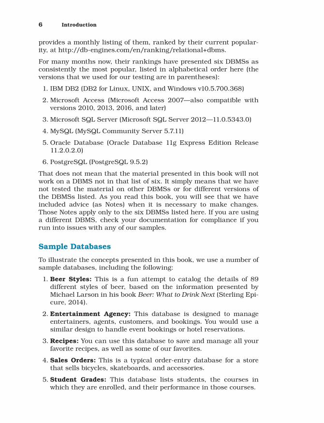
provides a monthly listing of them, ranked by their current popular-ity, at http://db-engines.com/en/ranking/relational+dbms.

For many months now, their rankings have presented six DBMSs as consistently the most popular, listed in alphabetical order here (the versions that we used for our testing are in parentheses):

1. IBM DB2 (DB2 for Linux, UNIX, and Windows v10.5.700.368)

2. Microsoft Access (Microsoft Access 2007—also compatible with versions 2010, 2013, 2016, and later)

3. Microsoft SQL Server (Microsoft SQL Server 2012—11.0.5343.0)

4. MySQL (MySQL Community Server 5.7.11)

5. Oracle Database (Oracle Database 11g Express Edition Release 11.2.0.2.0)

6. PostgreSQL (PostgreSQL 9.5.2)

That does not mean that the material presented in this book will not work on a DBMS not in that list of six. It simply means that we have not tested the material on other DBMSs or for different versions of the DBMSs listed. As you read this book, you will see that we have included advice (as Notes) when it is necessary to make changes. Those Notes apply only to the six DBMSs listed here. If you are using a different DBMS, check your documentation for compliance if you run into issues with any of our samples.

Sample Databases

To illustrate the concepts presented in this book, we use a number of sample databases, including the following:

1. Beer Styles: This is a fun attempt to catalog the details of 89 different styles of beer, based on the information presented by Michael Larson in his book Beer: What to Drink Next (Sterling Epi-cure, 2014).

2. Entertainment Agency: This database is designed to manage entertainers, agents, customers, and bookings. You would use a similar design to handle event bookings or hotel reservations.

3. Recipes: You can use this database to save and manage all your favorite recipes, as well as some of our favorites.

4. Sales Orders: This is a typical order-entry database for a store that sells bicycles, skateboards, and accessories.

5. Student Grades: This database lists students, the courses in which they are enrolled, and their performance in those courses.

Where to Find the Samples on GitHub 7

We also provide a number of sample databases specific to a particular item, some of which are built by a code listing within the item. The schemas and sample data are available in the GitHub site associated with the book.

Where to Find the Samples on GitHub

Many technical books come with a CD-ROM containing the examples in electronic form. That can be limiting, so we decided to provide our exam-ples in GitHub, at https://github.com/TexanInParis/Effective-SQL.

There, you will find high-level folders for each of the six DBMSs we considered. Within each of those high-level folders are ten folders cor-responding to the ten chapters in the book, plus a folder for the sam-ple databases.

Within each of the ten chapter folders, there are individual files, named to correspond to the listing numbers within each chapter. Note that not all listings are applicable to every DBMS. When that is the case, we highlight differences in the README files for each chap-ter. For Microsoft Access, the README file indicates which sample database contains the listings for the chapter.

The root folder on GitHub also contains the Listings.xlsx file that shows you which database contains each listing. That file also doc-uments SQL samples that are applicable to each of the six database systems.

Each of the sample database folders, with the exception of the Microsoft Access folder that contains .accdb files in 2007 format, contains a number of SQL files. We used the 2007 format for Microsoft Access because it is compatible over all versions of the product since version 12 (2007). One set of these files creates the structure for each sample database, and the other set of files contains the data to populate the sample databases. (Note that some of the items in this book rely on specific data cases. The structures and data for those items are sometimes contained within the chapter listings.)

NoteIn preparing the listings in this book for publication, we sometimes had issues fitting within the 63-character-per-line limit imposed by the phys-ical page. It is possible that a listing could have been edited incorrectly. When in doubt, all the listings on GitHub were tested, so we are confi-dent that they are correct.

8 Introduction

Summary of the Chapters

As the title of the book suggests, 61 specific items are presented in this book. Each item is intended to stand by itself; you should not need to read other items in order to use the material presented in a specific item. There are, of course, times when the material in a specific item does build on material in other items. When that is the case, we have tried to present as much background material as we felt was necessary, but we do provide cross-references to other relevant items so that you can review the material yourself.

Although each item is, as already stated, intended to stand alone, we felt there were natural groupings of topics. The groupings we used are these ten:

1. Data Model Design: Because you cannot write effective SQL when you are working with a bad data model design, the items in this chapter cover some basics of good relational model design. If your database design violates any of the rules discussed in this chapter, you need to figure out what is wrong and fix it.

2. Programmability and Index Design: Simply having a good logical data model design is not sufficient to allow you to write effective SQL. You must ensure that you have implemented the design in an appropriate manner, or you may find that your abil-ity to extract meaningful information from the data in an efficient manner using SQL will be compromised. The items in this chap-ter help you understand the importance of indexes, and how to ensure that they have been properly implemented.

3. When You Can’t Change the Design: Sometimes, despite your best efforts, you are forced to deal with external data outside of your control. The items in this chapter are intended to help you deal with such situations.

4. Filtering and Finding Data: The ability to look for or filter out the data of interest is one of the most important tasks you can do in SQL. The items in this chapter explore different techniques you can use to extract the exact information you want.

5. Aggregation: The SQL Standard has always provided the abil-ity to aggregate data. However, typically you are asked to provide “totals per customer,” “count of orders by day,” or “average sales of each category by month.” It is the part after the “per,” “by,” and “of each” that requires additional attention. The items in this chapter present techniques to get the best performance out of your aggre-gation. Some of them also show how to use window functions to provide even more complex aggregations.

Summary of the Chapters 9

6. Subqueries: There are many different ways in which you can use subqueries. The items in this chapter are intended to show a vari-ety of ways to get additional flexibility in your SQL through the use of subqueries.

7. Getting and Analyzing Metadata: Sometimes just data is not enough. You need data about data. You might even need data about how you are getting the data. In some cases, it might even be convenient to get the metadata using SQL. The items in this chapter tend to be quite product specific, but our hope is that we provide sufficient information so that you can apply the principles to your specific DBMS.

8. Cartesian Products: Cartesian Products are the result of com-bining all rows in one table with all rows in a second table. While perhaps not as common as other join types, the items in this chapter show real-world situations where it would not be possible to answer the underlying question without the use of a Cartesian Product.

9. Tally Tables: Another useful tool is the tally table, usually a table with a single column of sequential numbers, or a single column of sequential dates, or something more complex to aid in “pivoting” a set of summaries. While Cartesian Products are dependent on actual values in the underlying tables, tally tables allow you to cover all possibilities. The items in this chapter show examples of various problems that can be solved only through the use of a tally table.

10. Modeling Hierarchical Data: It is not uncommon to have to model hierarchical data in your relational database. Unfortu-nately, it happens to be one of SQL’s weaker areas. The items in this chapter are intended to help you make the trade-off between data normalization, and ease of querying and maintenance of metadata.

Each database system has a variety of functions that you can use to calculate or manipulate date and time values. Each database sys-tem also has its own rules regarding data types and date and time arithmetic. Because of the differences, we also included an Appen-dix, “Date and Time Types, Operations, and Functions,” to help you work with date and time values in your database system. We believe it accurately summarizes the data types and arithmetic operations supported, but we do recommend that you consult your database doc-umentation for the specific syntax to use with each function.

This page intentionally left blank

3 When You Can’t Change the Design

You have spent considerable time ensuring that you have a proper logical data model for your situation. You have worked hard to ensure that it has been implemented as an appropriate physical model. Unfortunately, you find that some of your data must come from a source outside your control.

This does not mean that you are doomed to have SQL queries that will not perform well. The items in this chapter are intended to help you understand some options you have to be able to work with that inappropriately designed data from other sources. We will consider both the case when you can create objects to hold the transforma-tions and the case when you must perform the transformation as part of the query itself.

Because you do not have control over the external data, there is noth-ing you can do to change the design. However, you can use the infor-mation in the items in this chapter to work with the DBAs and still end up with effective SQL.

Item 18: Use Views to Simplify What Cannot Be Changed

Views are simply a composition of a table in the form of a predefined SQL query on one or many tables or other views. Although they are simple, there is much merit to their use.

NoteMicrosoft Access does not actually have an object called a view, but saved queries in Access can be thought of as views.

You can use views to ameliorate some denormalization issues. You have already seen the denormalized CustomerSales table in Item 2,

80 Chapter 3 When You Can’t Change the Design

“Eliminate redundant storage of data items,” and how it should have been modeled as four separate tables (Customers, AutomobileModels, SalesTransactions, and Employees). You've also seen the Assignments table with repeating groups in Item 3, “Get rid of repeating groups,” that should have been modeled as two separate tables (Drawings and Predecessors). While working to fix such problems, you could use views to represent how the data should appear.

You can create different views of CustomerSales as shown in Listing 3.1.

Listing 3.1 Views to normalize a denormalized table

CREATE VIEW vCustomers ASSELECT DISTINCT cs.CustFirstName, cs.CustLastName, cs.Address, cs.City, cs.PhoneFROM CustomerSales AS cs;

CREATE VIEW vAutomobileModels ASSELECT DISTINCT cs.ModelYear, cs.ModelFROM CustomerSales AS cs;

CREATE VIEW vEmployees ASSELECT DISTINCT cs.SalesPersonFROM CustomerSales AS cs;

As Figure 3.1 shows, vCustomers would still include two entries for Tom Frank because two different addresses were listed in the original table. However, you have a smaller set of data to work with. By sorting the data on CustFirstName and CustLastName, you should be able to see the duplicate entry, and you can correct the data in the CustomerSales table.

Figure 3.1 Data for view vCustomers

You saw in Item 3 how to use a UNION query to “normalize” a table that contains repeating groups. You can use views to do the same thing, as shown in Listing 3.2.

Item 18: Use Views to Simplify What Cannot Be Changed 81

Listing 3.2 Views to normalize a table with repeating groups

CREATE VIEW vDrawings ASSELECT a.ID AS DrawingID, a.DrawingNumberFROM Assignments AS a;

CREATE VIEW vPredecessors ASSELECT 1 AS PredecessorID, a.ID AS DrawingID, a.Predecessor_1 AS PredecessorFROM Assignments AS aWHERE a.Predecessor_1 IS NOT NULLUNIONSELECT 2, a.ID, a.Predecessor_2FROM Assignments AS aWHERE a.Predecessor_2 IS NOT NULLUNIONSELECT 3, a.ID, a.Predecessor_3FROM Assignments AS aWHERE a.Predecessor_3 IS NOT NULLUNIONSELECT 4, a.ID, a.Predecessor_4FROM Assignments AS aWHERE a.Predecessor_4 IS NOT NULLUNIONSELECT 5, a.ID, a.Predecessor_5FROM Assignments AS aWHERE a.Predecessor_5 IS NOT NULL;

One point that needs to be mentioned is that although all the views shown previously mimic what the proper table design should be, they can be used only for reporting purposes. Because of the use of SELECT DISTINCT in the views in Listing 3.1, and the use of UNION in Listing 3.2, the views are not updatable. Some vendors allow you to work around this limitation by defining triggers on views (also known as INSTEAD OF triggers) so that you can write the logic for applying modifications made via the view to the underlying base table yourself.

NoteDB2, Oracle, PostgreSQL, and SQL Server allow triggers on views. MySQL does not.

Some other reasons to use views include the following:

■ To focus on specific data: You can use views to focus on spe-cific data and on specific tasks. The view can return all rows of a table or tables, or a WHERE clause can be included to limit the rows

82 Chapter 3 When You Can’t Change the Design

returned. The view can also return only a subset of the columns in one or more tables.

■ To simplify or clarify column names: You can use views to pro-vide aliases on column names so that they are more meaningful.

■ To bring data together from different tables: You can use views to combine multiple tables into a single logical record.

■ To simplify data manipulation: Views can simplify how users work with data. For example, assume you have a complex query that is used for reporting purposes. Rather than make each user define the subqueries, outer joins, and aggregation to retrieve data from a group of tables, create a view. Not only does the view simplify access to the data (because the underlying query does not have to be written each time a report is being produced), but it ensures consistency by not forcing each user to create the query. You can also create inline user-defined functions that logically operate as parameterized views, or views that have parameters in WHERE clause search conditions or other parts of the query. Note that inline table-valued functions are not the same as scalar functions!

■ To protect sensitive data: When the table contains sensitive data, that data can be left out of the view. For instance, rather than reveal customer credit card information, you can create a view that uses a function to “munge” the credit card numbers so that users are not aware of the actual numbers. Depending on the DBMS, only the view would be made accessible to users, and the underlying tables need not be directly accessible. Views can be used to provide both column-level and row-level security. Note that a WITH CHECK OPTION clause is necessary to protect the data integrity by preventing users from performing updates or deletes that go beyond the constraints imposed by the view.

■ To provide backward compatibility: Should changes be required to the schemas for one or more of the tables, you can create views that are the same as the old table schemas. Applications that used to query the old tables can now use the views, so that the application does not have to be changed, especially if it is only reading data. Even applications that update data can sometimes still use a view if INSTEAD OF triggers are added to the new view to map INSERT, DELETE, and UPDATE operations on the view to the underlying tables.

■ To customize data: You can create views so that different users can see the same data in different ways, even when they are using the same data at the same time. For example, you can create a

Item 18: Use Views to Simplify What Cannot Be Changed 83

view that retrieves only the data for those customers of interest to a specific user based on that user’s login ID.

■ To provide summarizations: Views can use aggregate functions (SUM(), AVERAGE(), etc.) and present the calculated results as part of the data.

■ To export and import data: You can use views to export data to other applications. You can create a view that gives you only the desired data, and then use an appropriate data utility to export just that data. You can also use views for import purposes when the source data does not contain all columns in the underlying table.

Do Not Create Views on ViewsIt is permissible to create a view that references another view(s). Those coming from a programming background might be tempted to treat a view the way they would treat a procedure in an imperative pro-gramming language. That is actually a big mistake and will cause more performance and maintenance problems, likely offsetting any savings gained from having a generic view that is then used as a base for other views. Listing 3.3 demonstrates an example of creating views on other views.

Listing 3.3 Three view definitions

CREATE VIEW vActiveCustomers ASSELECT c.CustomerID, c.CustFirstName, c.CustLastName, c.CustFirstName + ' ' + c.CustLastName AS CustFullNameFROM Customers AS cWHERE EXISTS (SELECT NULL FROM Orders AS o WHERE o.CustomerID = c.CustomerID AND o.OrderDate > DATEADD(MONTH, -6, GETDATE()));

CREATE VIEW vCustomerStatistics ASSELECT o.CustomerID, COUNT(o.OrderNumber) AS OrderCount, SUM(o.OrderTotal) AS GrandOrderTotal, MAX(o.OrderDate) AS LastOrderDateFROM Orders AS oGROUP BY o.CustomerID;

continues

84 Chapter 3 When You Can’t Change the Design

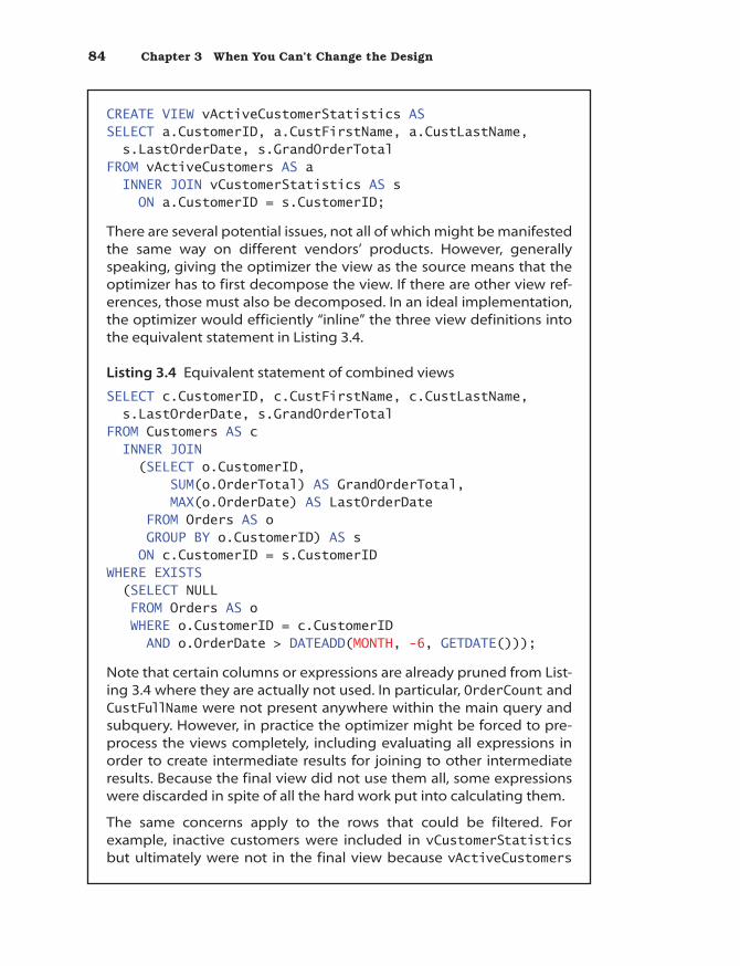
CREATE VIEW vActiveCustomerStatistics ASSELECT a.CustomerID, a.CustFirstName, a.CustLastName, s.LastOrderDate, s.GrandOrderTotalFROM vActiveCustomers AS a INNER JOIN vCustomerStatistics AS s ON a.CustomerID = s.CustomerID;

There are several potential issues, not all of which might be manifested the same way on different vendors’ products. However, generally speaking, giving the optimizer the view as the source means that the optimizer has to first decompose the view. If there are other view ref-erences, those must also be decomposed. In an ideal implementation, the optimizer would efficiently “inline” the three view definitions into the equivalent statement in Listing 3.4.

Listing 3.4 Equivalent statement of combined views

SELECT c.CustomerID, c.CustFirstName, c.CustLastName, s.LastOrderDate, s.GrandOrderTotalFROM Customers AS c INNER JOIN (SELECT o.CustomerID, SUM(o.OrderTotal) AS GrandOrderTotal, MAX(o.OrderDate) AS LastOrderDate FROM Orders AS o GROUP BY o.CustomerID) AS s ON c.CustomerID = s.CustomerIDWHERE EXISTS (SELECT NULL FROM Orders AS o WHERE o.CustomerID = c.CustomerID AND o.OrderDate > DATEADD(MONTH, -6, GETDATE()));

Note that certain columns or expressions are already pruned from List-ing 3.4 where they are actually not used. In particular, OrderCount and CustFullName were not present anywhere within the main query and subquery. However, in practice the optimizer might be forced to pre-process the views completely, including evaluating all expressions in order to create intermediate results for joining to other intermediate results. Because the final view did not use them all, some expressions were discarded in spite of all the hard work put into calculating them.

The same concerns apply to the rows that could be filtered. For example, inactive customers were included in vCustomerStatistics but ultimately were not in the final view because vActiveCustomers

Item 19: Use ETL to Turn Nonrelational Data into Information 85

Things to Remember

✦ Use views to structure data in a way that users will find natural or intuitive.

✦ Use views to restrict access to the data such that users can see (and sometimes modify) exactly what they need and no more. Remember to use WITH CHECK OPTION when necessary.

✦ Use views to hide and reuse complex queries.

✦ Use views to summarize data from various tables that can be used to generate reports.

✦ Use views to implement and enforce naming and coding standards, especially when working with legacy database designs that need to be updated.

Item 19: Use ETL to Turn Nonrelational Data into Information

Extract, Transform, Load (ETL) is a set of procedures or tools you can use to Extract data from an external source, Transform it to con-form to relational design rules or to conform to other requirements, then Load it into your database for further use or analysis. Nearly

excluded those customers. This can potentially result in far more I/Os than you anticipated. You can learn more about those considerations in Item 46, “Understand how the execution plan works.” Although this is a somewhat oversimplified example, it is fairly easy to create a view that the optimizer simply cannot inline when it is referenced in other views. Worse, there would be more than one way to create such views that would prevent inlining. Finally, the optimizer generally does a bet-ter job when it is given a simpler query expression that asks for exactly the data it actually needs.

For those reasons, it is best to avoid creating views on views. If you need a different presentation of the view, create a new view that directly references the base tables with the appropriate filters or groupings applied. You can also embed subqueries in a view, which can be useful in making the aggregated calculations “private” to the view. This approach helps to prevent proliferation of several views that are not directly usable, making the database solution much more maintainable. Refer to Item 42, “If possible, use common table expres-sions instead of subqueries,” for additional techniques.

86 Chapter 3 When You Can’t Change the Design

all database systems provide various utilities to aid in this process. These utilities are, quite simply, a means to convert raw data into information.

To get an idea of what these utilities can do, let’s take a look at some of the tools in Microsoft Access—one of the first Windows-era data-base systems to provide built-in ways to load and transform data into something useful. Assume you work as the marketing manager for a company that produces breakfast cereals. You need not only to ana-lyze competitive sales from another manufacturer but also to break down this analysis by individual brands.

You can certainly glean total sales information from publicly avail-able documents, but you really want to try to break down compet-itive sales by individual brand. To do this, you might strike up an agreement with a major grocery store chain to get them to provide their sales information by brand in return for a small discount on your products. The grocery chain promises to send you a spreadsheet containing sales data from all its stores broken down by competi-tive brand for the previous year. The data you receive might look like Table 3.1.

Table 3.1 Sample competitive sales data

Product Jan Feb Mar

Alpha-Bits 57775.87 40649.37 . . .

Golden Crisp 33985.68 17469.97 . . .

Good Morenings 40375.07 36010.81 . . .

Grape-Nuts 55859.51 38189.64 . . .

Great Grains 37198.23 41444.41 . . .

Honey Bunches of Oats 63283.28 35261.46 . . .

. . . additional rows . . .

It is clear that some blank columns that you do not need were added for readability. You also need to transform the data to end up with one row per product per month, and you have a separate table listing competitive products that has its own primary key, so you need to match on product name to get the key value to use as a foreign key.

Let’s start by extracting the data from the spreadsheet into a more usable form. Microsoft Access can import data in many different for-mats, so let’s fire up the Import tool to import a spreadsheet. In the

Item 19: Use ETL to Turn Nonrelational Data into Information 87

first step, you identify the file and tell Access what you want to do with the output (import into a new table, append the data to an exist-ing table, or link as a read-only table).

When you go to the next step, Access shows you a grid with a sample of the data it found, as shown in Figure 3.2. Because it determined that the first row might very well be usable as column names, it has used the names it found and has assigned generated names to the blank columns.

Figure 3.2 The Import Spreadsheet utility performing an initial analysis of the data

In the following step, Access shows you a display where you can select columns one at a time, tell Access to skip unimportant columns, and fix the data type that the utility has assumed. Figure 3.3 on the next page shows one of the data columns selected. The utility has assumed that the numbers, because they contain decimal points, should be imported as the very flexible Double data type. We know that these are all dollar sales figures, so it makes sense to change the data type to Currency to make it easier to work with the data. You can also see the “Do not import” check box (behind the drop-down) that you can select for columns that you want to ignore.

88 Chapter 3 When You Can’t Change the Design

The next step in the utility lets you pick a column to act as the pri-mary key, ask the utility to generate an ID column with incrementing integers, or assign no primary key to the table. The final step allows you to name the table (the default is the name of the worksheet) and to invoke another utility after importing the table to perform further analysis and potentially reload the data into a more normalized table design. If you choose to run the Table Analyzer, Access presents you with a design tableau as shown in Figure 3.4. In the figure, we have already dragged and dropped the Product column into a separate table and named both tables. As you can see, the utility automat-ically generates a primary key in the product table and provides a matching foreign key in the sales data table.

Even after using the Table Analyzer, you can see that there is still plenty of work to do to further normalize the sales data into one row per month. You can “unpivot” the sales data by using a UNION query to turn the columns into rows, as shown in Listing 3.5. (See also Item 21, “Use UNION statements to ‘unpivot’ non-normalized data.”)

Figure 3.3 Selecting columns to skip and choosing a data type

Item 19: Use ETL to Turn Nonrelational Data into Information 89

Listing 3.5 Using a UNION query to “unpivot” a repeating group

SELECT '2015-01-01' AS SalesMonth, Product, Jan AS SalesAmtFROM tblPostSalesUNION ALLSELECT '2015-02-01' AS SalesMonth, Product, Feb AS SalesAmtFROM tblPostSalesUNION ALL ... etc. for all 12 months.

The tools in Microsoft Access are fairly simple (for example, they can-not handle totals rows), but they give you an idea of the amount of work that can be saved when trying to perform ETL to load exter-nal data into your database. As noted earlier, most database systems provide similar—and in some cases more powerful—tools that you can use. Examples include Microsoft SQL Server Integration Services (SSIS), Oracle Data Integrator (ODI), and IBM InfoSphere DataStage. Commercial tools are available from vendors such as Informatica, SAP, and SAS, and you can also find a number of open-source tools available on the Web.

The main point here is that you should use those tools so that your data conforms to the data model that your business needs, not the

Figure 3.4 Using the Table Analyzer to break out products into a separate table

90 Chapter 3 When You Can’t Change the Design

other way around. A common mistake is to build tables that fit the incoming data as is and then use it directly in applications. The invest-ment made to transform data will result in a database that is easy to understand and maintain in spite of the divergent data sources from which it may collect the raw input.

Things to Remember

✦ ETL tools allow you to import nonrelational data into your database with less effort.

✦ ETL tools help you reformat and rearrange imported data so that you can turn it into information.

✦ Most database systems offer some level of ETL tools, and there are also commercial tools available.

Item 20: Create Summary Tables and Maintain Them

We mentioned previously (in Item 18, “Use views to simplify what can-not be changed”) that views can be used to simplify complex queries, and we even suggested that views can be used to provide summariza-tions. Depending on the volume of data, there are times when it may be more appropriate to create summary tables.

When you have a summary table, you can be sure that everything is in one place, making it easier to understand the data structure and quicker to return information.

One approach is to create a table that summarizes your data in your details table, and write triggers to update the summary table every time something changes in the details table. However, if your details table is frequently modified, this can be processor intensive.

Another approach is to use a stored procedure to refresh the sum-mary table on a regular basis: delete all existing data rows and rein-sert the summarized information.

DB2 has the concept of summary tables built into it. DB2 summary tables can maintain a summary of data in one or multiple tables. You have the option to have the summary refreshed every time the data in underlying table(s) changes, or you can refresh it manually. DB2 summary tables not only allow users to obtain results faster, but the optimizer can use the summary tables when user queries indirectly request information already summarized in the summary tables if ENABLE QUERY OPTIMIZATION is specified when you create the summary table. Although there may still be “costs” associated with all that

Item 20: Create Summary Tables and Maintain Them 91

activity, at least you did not have to write triggers or stored proce-dures to maintain the data for you.

Listing 3.6 shows how to create a summary table named SalesSummary that summarizes data from six different tables in DB2. Note that the SQL is not much different from that for creating a view. In fact, a summary table is a specific type of materialized query table, identi-fied by the inclusion of a GROUP BY clause in the CREATE SQL. Note that we had to use Cartesian joins with filters, because of the restriction against using INNER JOIN in a materialized query table, and addition-ally provide COUNT(*) in the SELECT list to enable the use of the REFRESH IMMEDIATE clause. Those are necessary to permit the optimizer to use it.

Listing 3.6 Creating a summary table based on six tables (DB2)

CREATE SUMMARY TABLE SalesSummary AS (SELECT t5.RegionName AS RegionName, t5.CountryCode AS CountryCode, t6.ProductTypeCode AS ProductTypeCode, t4.CurrentYear AS CurrentYear, t4.CurrentQuarter AS CurrentQuarter, t4.CurrentMonth AS CurrentMonth, COUNT(*) AS RowCount, SUM(t1.Sales) AS Sales, SUM(t1.Cost * t1.Quantity) AS Cost, SUM(t1.Quantity) AS Quantity, SUM(t1.GrossProfit) AS GrossProfitFROM Sales AS t1, Retailer AS t2, Product AS t3, datTime AS t4, Region AS t5, ProductType AS t6WHERE t1.RetailerId = t2.RetailerId AND t1.ProductId = t3.ProductId AND t1.OrderDay = t4.DayKey AND t2.RetailerCountryCode = t5.CountryCode AND t3.ProductTypeId = t6.ProductTypeIdGROUP BY t5.RegionName, t5.CountryCode, t6.ProductTypeCode, t4.CurrentYear, t4.CurrentQuarter, t4.CurrentMonth)DATA INITIALLY DEFERREDREFRESH IMMEDIATEENABLE QUERY OPTIMIZATIONMAINTAINED BY SYSTEMNOT LOGGED INITIALLY;

Listing 3.7 on the next page shows how to provide a similar capability in Oracle through the use of a materialized view.

92 Chapter 3 When You Can’t Change the Design

Listing 3.7 Creating a materialized view based on six tables (Oracle)

CREATE MATERIALIZED VIEW SalesSummary TABLESPACE TABLESPACE1 BUILD IMMEDIATE REFRESH FAST ON DEMANDASSELECT SUM(t1.Sales) AS Sales, SUM(t1.Cost * t1.Quantity) AS Cost, SUM(t1.Quantity) AS Quantity, SUM(t1.GrossProfit) AS GrossProfit, t5.RegionName AS RegionName, t5.CountryCode AS CountryCode, t6.ProductTypeCode AS ProductTypeCode, t4.CurrentYear AS CurrentYear, t4.CurrentQuarter AS CurrentQuarter, t4.CurrentMonth AS CurrentMonthFROM Sales AS t1 INNER JOIN Retailer AS t2 ON t1.RetailerId = t2.RetailerId INNER JOIN Product AS t3 ON t1.ProductId = t3.ProductId INNER JOIN datTime AS t4 ON t1.OrderDay = t4.DayKey INNER JOIN Region AS t5 ON t2.RetailerCountryCode = t5.CountryCode INNER JOIN ProductType AS t6 ON t3.ProductTypeId = t6.ProductTypeIdGROUP BY t5.RegionName, t5.CountryCode, t6.ProductTypeCode, t4.CurrentYear, t4.CurrentQuarter, t4.CurrentMonth;

Although SQL Server does not directly support materialized views, the fact that you can create indexes on views has a similar effect, and thus you can use indexed views in a similar manner.

NoteVarious vendors implement additional restrictions. We advise first con-sulting your documentation to determine what is actually supported before creating a summary table/materialized view/indexed view.

Note that there can be some negative aspects to summary tables as well, such as the following:

■ Each summary table occupies storage.

■ The administrative work (triggers, constraints, stored procedures) may need to exist on both the original table and any summary tables.

Item 20: Create Summary Tables and Maintain Them 93

■ You need to know in advance what users want to query in order to precompute the required aggregations and include them in the summary tables.

■ You may need multiple summary tables if you need different groupings or filters applied.

■ You may need to set up a schedule to manage the refresh of the summary tables.

■ You may need to manage the periodicity of the summary tables via SQL. For example, if the summary table is supposed to show the past 12 months, you need a way to remove data that is more than a year old from the table.

One possible suggestion to avoid some of the increased administrative costs of having redundant triggers, constraints, and stored proce-dures is to use what Ken Henderson referred to as inline summari-zation in his book The Guru’s Guide to Transact-SQL (Addison-Wesley, 2000). This involves adding aggregation columns to the existing table. You would use an INSERT INTO SQL statement to aggregate data and store those aggregations in the same table. Columns that are not part of the aggregated data would be set to a known value (such as NULL or some fixed date). An advantage of doing inline summariza-tion is that the summary and the detail data can be easily queried together or separately. The summarized records are easily identified by the known values in certain columns, but other than that, they are indistinguishable from the detail records. However, this approach necessitates that all queries on the table containing both detail and summary data be written appropriately.

Things to Remember

✦ Storing summarized data can help minimize the processing required for aggregation.

✦ Using tables to store the summarized data allows you to index fields containing the aggregated data for more efficient queries on aggregates.

✦ Summarization works best on tables that are more or less static. If the source tables change too often, the overhead of summarization may be too great.

✦ Triggers can be used to perform summarization, but a stored proce-dure to rebuild the summary table is usually better.

94 Chapter 3 When You Can’t Change the Design

Item 21: Use UNION Statements to “Unpivot” Non-normalized Data

You saw in Item 3, “Get rid of repeating groups,” how UNION queries can be used to deal with repeating groups. We explore UNION queries a little bit more in this item. As you will learn in Item 22, “Understand relational algebra and how it is implemented in SQL,” the Union oper-ation is one of the eight relational algebra operations that can be per-formed within the relational model defined by Dr. Edgar F. Codd. It is used to merge data sets created by two (or more) SELECT statements.

Assume that the only way you are able to get some data for analysis is in the form of the Excel spreadsheet pictured in Figure 3.5, which is obviously not normalized.

Figure 3.5 Non-normalized data from Excel

Assuming you can import that data into your DBMS, at best you will end up with a table (SalesSummary) that has five pairs of repeating groups, which we will call OctQuantity, OctSales, NovQuantity, NovSales, and so on to FebQuantity and FebSales.

Listing 3.8 shows a query that would let you look at the October data.

Listing 3.8 SQL to extract October data

SELECT Category, OctQuantity, OctSalesFROM SalesSummary;

Of course, to look at the data for a different month, you need a dif-ferent query. And let’s not forget that data that is not normalized can be more difficult to use for analysis purposes. This is where a UNION query can help.

Item 21: Use UNION Statements to “Unpivot” Non-normalized Data 95

There are three basic rules that apply when using UNION queries:

1. There must be the same number of columns in each of the queries making up the UNION query.

2. The order of the columns in each of the queries making up the UNION query must be the same.

3. The data types of the columns in each of the queries must be compatible.

Note that there is nothing in those rules about the names of the col-umns in the queries that make up the UNION query.

Listing 3.9 shows how to combine all of the data into a normalized view.

Listing 3.9 Using UNION to normalize the data

SELECT Category, OctQuantity, OctSalesFROM SalesSummaryUNIONSELECT Category, NovQuantity, NovSalesFROM SalesSummaryUNIONSELECT Category, DecQuantity, DecSalesFROM SalesSummaryUNIONSELECT Category, JanQuantity, JanSalesFROM SalesSummaryUNIONSELECT Category, FebQuantity, FebSalesFROM SalesSummary;

Table 3.2 shows a partial extract of the data returned.

Table 3.2 Partial extract of data returned by the UNION query in Listing 3.9

Category OctQuantity OctSales

Accessories 923 60883.03

Accessories 930 61165.40

. . . . . . . . .

Bikes 450 585130.50

Bikes 542 705733.50

continues

96 Chapter 3 When You Can’t Change the Design

Two things should stand out. First, there is no way to distinguish to which month the data applies. The first two rows, for instance, represent the quantity and sales amount for Accessories for October and November, but there is no way to tell that from the data. As well, despite the fact that the data represents five months of sales, the col-umns are named OctQuantity and OctSales. That is because UNION queries get their column names from the names of the columns in the first SELECT statement.

Listing 3.10 shows a query that remedies both of those issues.

Listing 3.10 Tidying up the UNION query used to normalize the data

SELECT Category, 'Oct' AS SalesMonth, OctQuantity AS Quantity, OctSales AS SalesAmtFROM SalesSummaryUNIONSELECT Category, 'Nov', NovQuantity, NovSalesFROM SalesSummaryUNIONSELECT Category, 'Dec', DecQuantity, DecSalesFROM SalesSummary

Category OctQuantity OctSales

Car racks 96 16772.05

Car racks 115 20137.05

Car racks 124 21763.30

. . . . . . . . .

Skateboards 203 89040.58

Skateboards 204 79461.30

Tires 110 3081.24

Tires 137 3937.70

Tires 150 4388.55

Tires 151 4356.91

Tires 186 5377.60

Table 3.2 Partial extract of data returned by the UNION query in Listing 3.9 (continued )

Item 21: Use UNION Statements to “Unpivot” Non-normalized Data 97

UNIONSELECT Category, 'Jan', JanQuantity, JanSalesFROM SalesSummaryUNIONSELECT Category, 'Feb', FebQuantity, FebSalesFROM SalesSummary;

Table 3.3 shows the same partial extract returned by the query in Listing 3.10.

Table 3.3 Partial extract of data returned by the UNION query in Listing 3.10

Category SalesMonth Quantity SalesAmount

Accessories Dec 987 62758.14

Accessories Feb 979 60242.47

. . . . . . . . . . . .

Bikes Nov 412 546657.00

Bikes Oct 413 536590.50

Car racks Dec 115 20137.05

Car racks Feb 124 21763.30

Car racks Jan 142 24794.75

. . . . . . . . . . . .

Skateboards Nov 203 89040.58

Skateboards Oct 164 60530.06

Tires Dec 150 4388.55

Tires Feb 137 3937.70

Tires Jan 186 5377.60

Tires Nov 110 3081.24

Tires Oct 151 4356.91

Should you want the data presented in a different sequence, the ORDER BY clause must appear after the last SELECT in the UNION query, as shown in Listing 3.11 on the next page.

98 Chapter 3 When You Can’t Change the Design

Listing 3.11 Specifying the sort order of the UNION query

SELECT Category, 'Oct' AS SalesMonth, OctQuantity AS Quantity, OctSales AS SalesAmtFROM SalesSummaryUNIONSELECT Category, 'Nov', NovQuantity, NovSalesFROM SalesSummaryUNIONSELECT Category, 'Dec', DecQuantity, DecSalesFROM SalesSummaryUNIONSELECT Category, 'Jan', JanQuantity, JanSalesFROM SalesSummaryUNIONSELECT Category, 'Feb', FebQuantity, FebSalesFROM SalesSummaryORDER BY SalesMonth, Category;

Table 3.4 shows a partial extract returned by the query in Listing 3.11.

Table 3.4 Partial extract of data returned by the UNION query in Listing 3.11

Category SalesMonth Quantity SalesAmount

Accessories Dec 987 62758.14

Bikes Dec 332 439831.50

Car racks Dec 115 20137.05

Clothing Dec 139 4937.74

Components Dec 265 27480.22

Skateboards Dec 129 59377.20

Tires Dec 150 4388.55

Accessories Feb 979 60242.47

Bikes Feb 450 585130.50

Car racks Feb 124 21763.30

. . . . . . . . . . . .

Item 21: Use UNION Statements to “Unpivot” Non-normalized Data 99

NoteSome DBMSs (such as Microsoft Access) allow you to put ORDER BY clauses other than at the end, but they do not actually cause the order to change.

When specifying the columns in the ORDER BY clause, usually you have the option of referring to them by name (remembering that the column names are specified in the first SELECT ) or by position number. In other words, List-ing 3.11 could use ORDER BY 2, 1 instead of ORDER BY SalesMonth, Category. Oracle, however, insists on using ordinal references.

Another consideration is that UNION queries eliminate any dupli-cate rows. Should this not be what you want, you can specify UNION ALL instead of UNION, and duplicates will not be eliminated. On the other hand, UNION ALL can provide performance improvements as it skips the step of deduplicating the result set, so if you know that the sources will not overlap, it can be advantageous to specify UNION ALL for those queries.

Things to Remember

✦ Each of the SELECT statements in the UNION query must have the same number of columns.

✦ Although the names of the columns in the various SELECT statements do not matter, the data types of each column must be compatible.

✦ To control the order in which the data appears, you can use an ORDER BY clause after the last SELECT statement.

✦ Use UNION ALL rather than UNION if you do not wish to eliminate duplicate rows or pay the performance penalty of deduplicating rows.

This page intentionally left blank

Index

Symbols& (ampersand) operator, concatenation

symbol, 24, 249+ (plus sign) operator, concatenation

symbol, 24, 249|| (vertical bars) operator, concatenation

symbol, 24, 248–249

AAbsent data. See Null values.Access

choosing a primary key, 88Edit Relationships dialog box, 64execution plans, 204–205, 212ignoring columns, 87–88importing data, 86–87naming tables, 88support for CTEs, 249tools, 86–89unpivoting sales data, 88–89upsizing from, 63–64

Access, date and timearithmetic operations, 303–304data types, 303functions, 304–305

Accumulating snapshot fact tables, 46Adjacency list model, hierarchical data,

286–288Age calculation, SQL code example, 113Aggregation

counting items in a group, 156–159distinct counts, 163–166finding maximum/minimum values,

150–155moving aggregates, 172–177partitioning data into groups. See

GROUP BY clause.running sums, calculating, CTEs,

166–169

setting bounds for window frames, CTEs, 172–177

sizing window frames, CTEs, 172–177solving complex problems, 145–150

Aggregation, rowsAdjacent, CTEs, 166–169contiguous ranking, CTEs, 169–172counting, 137gaps in rankings, CTEs, 171–172numbering, CTEs, 169–172physical grouping. See RANGE

keyword.physical offsets. See ROWS keyword.ranking, CTEs, 169–172

Ampersand (&) operator, concatenation symbol, 24, 249

ANALYZE option, 210Ancestry traversal, hierarchical data,

294–298ANSI (American National Standards

Institute), 3ANSI NCITS-H2 organization, 5ANSI X3.135-1986 Database Language

SQL standard, 3–4Appointment calendar, creating, 275–277Arvin, Troels, 70, 72AS clause, 26AS keyword, 26Atomic data, 21Attributes, 21, 101. See also Columns.Averaging values, 137AVG() function, 137

BBidirectional indexes, 60Books and publications. See also Online

resources.Database Design for Mere Mortals,

11, 19

318 Index

Books and publications (continued )Handbook of Relational Database

Design, 19The Relational Model for Database

Management, 120SQL Queries for Mere Mortals, Third

Edition, 113BOOLEAN data type, null values, 71–72Boyce-Codd normal form, 38B-tree structure, 54–55, 60, 218Buffer usage, displaying, 210BUFFERS option, 210

CCalculated columns

attaching a trigger, 26for DB2, listing, 28defining columns, 26drawbacks, 29indexing, 29for Oracle, listing, 28overview, 25–29sample table definition, 25, 27, 28

Calculated datacalculating combinations for N items,

237calculating values across entire sets,

145–150example of SQL code, 25indexing results, 74–77storing, 45

Calendar, creating, 275–277Cartesian Products

calculating the combinations for N items, 237

combining rows between two tables, 227–230

creating combinations of things, 239description, 105–106finding partial matches, 240–245pairing rows in a table with all other

rows, 235–240ranking importance of qualifications,

240–245ranking rows by equal quantiles,

231–235Cascading updates, primary keys, 13CASE statements

overview, 110–114predicates, 111search conditions, 111searched, 111simple, 111

SQL code example, 111–113value expressions, 111

Celko, Joe, 123Chamberlin, Donald, 2CHECK constraint, 69Clustered indexes, 55Codd, Edgar F., 1, 101, 120Columns. See also Calculated columns.

adding/removing, 19–20getting, 102grouping, 136ignoring in Access, 87–88names, simplifying or clarifying with

views, 82one property per column, 21–25selecting, 102

Combinations for N items, calculating, 237

Combining rows, 105–106, 227–230. See also Cartesian Products.

Combining things, uses for, 239Common table expressions (CTEs). See

CTEs (common table expressions).Compound primary keys, 14CONCAT() function

databases supporting, 24listing, 24nesting, 24support for, 248–249

Constraints on table dataCHECK constraint, 69DEFAULT clause, 69default values for fields, 69FOREIGN KEY constraint, 68foreign keys for referential integrity,

68limiting fields to specified values, 69NOT NULL, 68PRIMARY KEY constraint, 68UNIQUE constraint, 68, 73unique record identity, 68, 73

Converting values, based on values in a tally table, 261–268

Correlated subqueries, 184–189Cost estimates, displaying, 210COSTS option, 210COUNT() function

Access restrictions, 166counting items in a group, 163–166dealing with zero values, 159–163description, 137distinct counts, 163–166erroneous messages, 156–159

Index 319

Countingdistinct counts, 163–166items in a group, 156–159, 163–166

CROSS JOIN keywords, 106CROSSTAB, 280CTEs (common table expressions)

in Access, 249in MySQL, 249recursive, 194–196SQL code example, 148–150in subqueries, SQL code example,

191–193traversing a hierarchy, SQL code

example, 194–195CTEs (common table expressions),

aggregationrunning sums, calculating, 166-169setting bounds for window frames,

172-177sizing window frames, 172-177

CTEs (common table expressions), aggregation, rows

Adjacent, 166-169contiguous ranking, 169-172gaps in rankings, 171-172numbering, 169-172ranking, 169-172

CUBE clause, 138–139CURRENT_DATE() function, 299CURRENT_TIME() function, 299CURRENT_TIMESTAMP() function, 299

D\d command, DB2, 217Data about data. See Metadata.Data clustering, indexes, 58Data manipulation, with views, 82Data sets, linking, 102–103Database 2 (DB2). See DB2 (Database

2).Database Design for Mere Mortals, 11, 19Database information, online resources,

5–6Database rankings, online resources, 6Databases. See also specific databases.

adding/removing data, 19–20normalization. See Normalization.samples used in examples, 6–7used in this book, summary of, 6–7

Date, Chris, 4, 122Date and time

CURRENT_DATE() function, 299, 299CURRENT_TIME() function, 299, 299

CURRENT_TIMESTAMP() function, 299, 299DATEADD() function, 27, 27in filtered or partial indexes, 67SQL standard functions, 299, 299time, handling in denormalization, 45

Date and time, Accessarithmetic operations, 303–304data types, 303functions, 304–305

Date and time, DB2arithmetic operations, 299–300data types, 299functions, 300–303

Date and time, MySQLarithmetic operations, 308–309data types, 308functions, 310–312

Date and time, Oraclearithmetic operations, 313data types, 313functions, 313–314

Date and time, PostgreSQLarithmetic operations, 315data types, 315functions, 315–316

Date and time, SQL Serverarithmetic operations, 306data types, 305functions, 306–308

Date calculations with tally tables, 268–274

Date tablesappointment calendar, creating,

275–277optimizing queries, 273–274simplifying date calculation, 268–274

DATEADD() function, 27–28DB2 (Database 2)

execution plans, 202–203, 212getting metadata, 217history of SQL, 3

DB2 (Database 2), date and timearithmetic operations, 299–300data types, 299functions, 300–303

db2look command, DB2, 217DB-Engines, online resources, 5–6Declarative Referential Integrity (DRI),

31DECODE, 279–280DEFAULT clause, 69Default values for fields, 69Delete anomalies, 16

320 Index

Denormalization, for information warehouses. See also Normalization.

accumulating snapshot fact tables, 46adding indicative fields to tables, 45avoiding a join, 44documenting, 46drilling across, 45drilling down, 45fact tables, 45–46handling time, 45overview, 43–46periodic snapshot fact tables, 45repeating groups, 45replicating identity fields in tables,

44slowly changing dimensions, 46storing calculated values, 45transaction fact tables, 45

DENSE_RANK() function, CTEs, 170–171Depth vs. distance, 296DESCRIBE command, Oracle, 217Deterministic functions, vs.

nondeterministic, 26–28Difference operation, 106–108Distance vs. depth, 296Distinct counts, 163–166DISTINCT keyword, 163–166Divide operation

description, 106SQL code example, 122–123

Dividing sets, 106Documenting, denormalization, 46DRI (Declarative Referential Integrity), 31Drilling across, 45Drilling down, 45Duplicate rows, eliminating, 99Duplicate values, preventing with

primary keys, 14

E“Elephant and mouse” problem,

223–224Empty grouping sets, 138Enforced RI, 13, 30–33Error messages, COUNT() function,

156–158ETL (Extract, Transform, Load), 85–90Examples of SQL code

age calculation, 76, 113appointment calendar, creating,

275–277CASE statements, 110–114

case-insensitive queries, 75complex GROUP BY clause, 144concatenation, 24converting values based on values in

a tally table, 261–267correlated subqueries, 188–189CUBE clause, sample query, 139date calculations, 268–271date tables, 268–271, 273–274defining columns, 28Difference operation, 107Divide operation, 122–123DRI for self-referencing relationship, 65EXCLUDE NULL KEYS option, 48, 49existence check, 109EXISTS clause, 198–199EXISTS operator, 109filtered indexes, 66–67filtering date ranges, 124–127filtering the right side of a left join,

132–134finding missing data, 114frustrated join, 109function definition for SQL Server, 27generating a list of numbers, 194generating multiple rows, 259–260GROUPING SETS clause, sample query, 140IGNORE NULL option, 50index creation, 59indexes on a table, 53inline expressions for Oracle, 28INNER JOIN, emulating an Intersect

operation, 105Intersect operation, 104–105joining a table to itself, 153LEFT JOIN clause, 153, 199mailing labels, skipping blank rows,

248–250maximum/minimum values, finding,

152–155non-correlated subqueries, 185–187nondeterministic function, 76non-sargable queries, 129–131normalizing data, 20NOT IN operator, 108null values in Access, 50null values in Oracle, 51–52one property per column, 22, 23optimizing queries with date tables,

273–274pivoting data, 279–282querying metadata, 213–216RANK() function, 170

Index 321

returning original data, 18, 24ROLLUP clause, sample query, 139ROW_NUMBER() function, 170rows, numbering and ranking, 170running sums, calculating, 166–169sample databases used in, 6–7sargable queries, 129–131scalar subqueries, 183–184separating attributes, 23sequencing data, 254–256solving multiple-criteria problems,

115–120sort operations, 67splitting into tables by subject, 17summarizing data with tally tables,

262–266summary tables, 91–92syntax for SQL SELECT statements,

136table creation, 59table subqueries, 180–181table with only one column

subqueries, 182–183totals query, 59triggers, 61–65using LIKE in the WHERE clause, 58views, 80–81, 121–122WHERE clause, 60

Examples of SQL code, Cartesian Products

combining rows between two tables, 228–229

finding partial matches, 242–244pairing rows in a table with all other

rows, 235–240ranking rows by equal quantiles,

232–233Examples of SQL code, COUNT() function

counting items in a group, 163–166dealing with zero values, 159–163description, 137erroneous messages, 156–159

Examples of SQL code, creating execution plans

Access, 204–205DB2, 202MySQL, 207Oracle, 208PostgreSQL, 210

Examples of SQL code, creating tablesfor calculated data, 25for Customers, 31for Orders, 32

with relationships, 36with separate attributes, 23for SQL Server, 27

Examples of SQL code, CTEssolving complex problems, 148–150in subqueries, 191–193traversing a hierarchy, 194–195

Examples of SQL code, excluding null values in

PostgreSQL, 52SQL Server, 50UNIQUE indexes, 48, 49

Examples of SQL code, GROUP BY clauseinstead of GROUPING SETS clause, 140solving complex problems, 145–150SQL standards compliance, 143–144valid vs. invalid, 137–138

Examples of SQL code, HAVING clausecounting zero-value rows, 160–163finding items by category, 148–150solving complex problems, 145–150

Examples of SQL code, modeling hierarchical data

adjacency list model, 286–288ancestry tables, 294–297getting all ancestors, 290, 293, 297getting all children, 290, 292,

296–297improving query performance,

290–291materialized path, 291–293nested lists, 290–291

Examples of SQL code, UNION queriesnormalizing data, 20, 95–96specifying sort order, 98

Examples of SQL code, window functions

moving aggregates, 172–177running sums, 167–168, 172–173

EXCLUDE NULL KEYS option, 48–49Execution plans

Access, 204–205, 212DB2, 202–203, 212“elephant and mouse” problem,

223–224functional description, 217–224MySQL, 207Oracle, 208–209, 212Showplan Capturer tool, 205SQL Server, 205–206, 212

Execution plans, PostgreSQLbuffer usage, displaying, 210cost estimates, displaying, 210

322 Index

Execution plans (continued )description, 209–212output format, specifying, 210performance statistics, displaying, 210timing information, displaying, 210

Existence check, 109EXISTS operator, 109, 198–199EXPLAIN option, 209–210Exporting/importing data

Access, 86–87with views, 83

Extensions, SQL, 5Extract, Transform, Load (ETL), 85–90

FFact tables, 45–46Fields, limiting to specified values, 695NF (fifth normal form), 37–43Filtered indexes, including/excluding

subsets of data, 65–68Filtering data. See also Finding data.

aggregate data, 138, 141, 145date ranges, 124–127right side of a left join, 132–134the right side of a left join, SQL code

example, 132–134rows, 102

Finding data. See also Filtering data.Divide operation, 120–123items by category, 148–150maximum/minimum values, 137,

150–155missing data, SQL code example, 114missing records, 108–110multiple-criteria problems, 115–120non-matches, 108–110partial matches, 240–245. See also

Cartesian Products.perfect matches, 120–123

Fleming, Candace C., 19FOREIGN KEY constraints, 17–18, 32–33, 68Foreign keys

defining FOREIGN KEY constraints, 32–33

enforcing RI, 30–33for referential integrity, 68

FORMAT option, 210Frustrated join, SQL code example, 109Functional dependency, 143Function-based indexes, 75–77Functions

for aggregation, 136–137inlining, 251

as parameterized views, 251returning entire tables, 251table-valued, 251

Functions, date and timeAccess, 304–305DB2, 300–303MySQL, 310–312Oracle, 313–314PostgreSQL, 315–316SQL Server, 306–308

GGENERATED keyword, 27–28Generating

lists of numbers, SQL code example, 194

rows with tally tables, 257–261running sums, 167–169

GitHub, online resources, 7Gosson, Stephen, 11GROUP BY clause. See also Aggregation.

aggregate functions, 136–137. See also specific functions.

averaging values, 137calculating values across entire sets,

145–150complex, SQL code example, 144counting rows, 137empty grouping sets, 138filtering aggregate data, 138, 141, 145finding largest/smallest value, 137functional dependency, 143grouping columns, 136keeping it small, 142–145ordering result sets, 138overview, 135–142population standard deviation,

calculating, 137population variance, calculating, 137

GROUP BY clause (conutinued )sample standard deviation,

calculating, 137sample variance, calculating, 137solving complex problems, 145–150summing values, 137

Grouping columns, 136GROUPING SETS clause, 138–140The Guru’s Guide to Transact-SQL, 93

HHandbook of Relational Database Design,

19Handling time, 45

Index 323

Hash joins, indexes, 57HAVING clause

comparing aggregate values, 145–150

counting zero-value rows, 159–163filtering aggregate data, 138finding items by category, 148–150generated in Access queries, 141solving complex problems, 145–150

Help. See Books and publications; Online resources.

Henderson, Ken, 93Hernandez, Michael J., 11, 19, 113Hierarchical data, modeling. See

Modeling hierarchical data.History of SQL

ANSI NCITS-H2 organization, 5Chamberlin, Donald, 2Codd, Edgar F., 1Date, Chris, 4DB2, 3extensions, 5IBM, 1–3Ingres, 2–3NCITS (National Committee for

Information Technology Standards), 5

Oracle, 2QUEL (Query Language), 2–3relational database model, 1–2Relational Software, Inc., 2Relational Technology, Inc., 3SEQUEL (Structured English Query

Language), 2SEQUEL/2, 2SEQUEL-XRM, 2SQL (structured query language), 2SQL/DS (SQL/Data System), 3standards, 3–5. See also specific

standards.Stonebraker, Michael, 2Wong, Eugene, 2X3H2 database technical committee,

3, 5

IIBM, in the history of SQL, 1–3IBM DB2. See DB2.IBM products. See specific products.IF ... THEN ... ELSE statements. See CASE

statements.Importing data. See Exporting/

importing data.

Inconsistent data, eliminating redundant storage, 15–19

Index scans, 52–56Indexes

bidirectional, 60B-tree structure, 54–55, 60on calculated results, 74–77clustered, 55combination of columns, 56data clustering, 58effects of table size, 55–56filtered, 65–68. See also Partitioned

tables.function-based, 75–77hash joins, 57index scans, 52–56join efficiency, 57–58most common type, 54–55nested loops, 57nonclustered, 55non-sargable queries, 128null values, 47–52ORDER BY clause, efficiency, 60partial, 65–68performance issues, 54pipelining, 60sargable queries, 127–131sort-merge joins, 57table scans, 52–56tuning queries, 52–56WHERE clause, efficiency, 56

Indexing calculated columns, 29INFORMATION_SCHEMA, 212–217

getting database metadata, 212–217getting object schemas, 217

InfoSphere DataStage, tools, 89Ingres, in the history of SQL, 2–3Inlining functions, 251INNER JOIN, 103, 105Insert anomalies, 15–16Intersect operation, SQL code example,

104–105IS NULL predicate, 47ISO 9075:1989 Database Language

SQL with Integrity Enhancement standard, 4

ISO 9075:1987 Database Language SQL standard, 4

ISO/IEC 9075-11:2011 Part 11: Information and Definition Schemas, 212

ISO/IEC 9075:1992 Database Language SQL standard, 4–5

324 Index

JJoin efficiency, indexes, 57–58JOIN keyword

description, 102–103instead of subqueries, 197–199vs. subqueries, 197–199

Join operationsavoiding, 44filtering the right side of a left join,

132–134frustrated, 109INNER JOIN, 103JOIN keyword, 102–103joining a table to itself, SQL code

example, 153NATURAL JOIN, 103OUTER JOIN, 103overview, 102–103sort-merge, 57

KKimball, Ralph, 45–46

LLEFT JOIN clause, SQL code example,

153, 199Listings of SQL code. See Examples of

SQL code.Lossless decomposition, 42

MMailing labels

generating blank rows, 248–250printing, 247–250

Materialized path, 291–294MAX() function, 137Maximum/minimum values, finding

MAX() function, 137MIN() function, 137SQL code example, 152–155without using GROUP BY, 150–155

Merging sets, 106Metadata, getting

\d command, DB2, 217DB2, 217db2look command, DB2, 217DESCRIBE command, Oracle, 217INFORMATION_SCHEMA, 212–217MySQL, 217Oracle, 217PostgreSQL, 217SHOW command, MySQL, 217

Microsoft Access. See Access.

Microsoft products. See specific products.

Microsoft SQL Server. See SQL Server.MIN() function, 137Minimum values, finding. See

Maximum/minimum values, finding.

Modeling hierarchical dataadjacency list model, 286–288ancestry traversal, 294–298complex searching, 294–298improving query performance,

288–291materialized path, 291–294nested lists, 288–291nodes, depth vs. distance, 296overview, 286traversing a hierarchy with CTEs,

194–195Moving aggregates, CTEs, 172–177MySQL

execution plans, 207getting metadata, 217support for CTEs, 249

MySQL, date and timearithmetic operations, 308–309data types, 308functions, 310–312

NNaming tables, Access, 88NATURAL JOIN, 103NCITS (National Committee for

Information Technology Standards), 5

Nested lists, 288–291Nested loops, indexes, 57Nesting, CONCAT() functions, 24Nodes, depth vs. distance, 296Nonclustered indexes, 55Non-correlated subqueries, 184–189Non-sargable queries, SQL code

example, 129–131Normal forms, 37–43Normalization. See also

Denormalization.3NF, 37–435NF, 37–436NF, 37–43Boyce-Codd normal form, 38columns, adding/removing, 19–20database samples, for scheduling, 41definition, 15

Index 325

delete anomalies, 16foreign key constraints, 17–18goal of, 15insert anomalies, 15–16lossless decomposition, 42normal forms, 37–43recreating original data, 17–18redundant storage, 15–19repeating groups, eliminating, 19–21rows, adding/removing, 20splitting into tables by subject, 17UNION queries, 20–21update anomalies, 16

NOT IN operator, 108NOT NULL constraint, 68Null values

in Access, 49–50BOOLEAN data type, 71–72in DB2, 48–49detecting, 47eliminating in UNIQUE indexes,

48–49in indexes, 47–52in MySQL, 51in Oracle, 51–52ordering, 70–71in PostgreSQL, 52in primary keys, 48SQL dialects, 70–71in SQL Server, 50testing for, 111

Numbers, generating a list of, 194Numeric primary keys, 14

OODI (Oracle Data Integrator), tools, 89Online resources. See also Books and

publications.for database information, 5–6database rankings, 6DB-Engines, 5–6GitHub, 7sample databases, 7SQL dialects, 70

Oracleexecution plans, 208–209, 212getting metadata, 217in the history of SQL, 2

Oracle, date and timearithmetic operations, 313data types, 313functions, 313–314

Oracle Data Integrator (ODI), tools, 89

ORDER BY clausegenerating a running sum, 167–169index efficiency, 60ordering result sets, 138

Ordering result sets, 138Orphan records, preventing, 61OUTER JOIN

counting items in a group, 156–159description, 103erroneous COUNT() messages, 156–159

Output format, specifying, 210OVER clause, generating a running sum,

167–169

PPairing rows in a table with all other

rows, 235–240. See also Cartesian Products.

Papers. See Books and publications.Partial indexes, 65–68PARTITION BY predicate

generating a running sum, 167–169grouping ranking functions, 170

Partitioned tables, 66Partitioning data into groups. See GROUP

BY clause.Performance

improving in modeling hierarchical data, 288–291

indexes, 54queries. See Execution plan.statistics, displaying, 210

Periodic snapshot fact tables, 45PERSISTED keyword, 29Pipelining, indexes, 60PIVOT, 280Pivoting data

definition, 278with tally tables, 278–283

Plus sign (+) operator, concatenation symbol, 24, 249

Population standard deviation, calculating, 137

Population variance, calculating, 137PostgreSQL, date and time

arithmetic operations, 315data types, 315functions, 315–316

PostgreSQL, execution plansbuffer usage, displaying, 210cost estimates, displaying, 210description, 209–212output format, specifying, 210

326 Index

PostgreSQL (continued )performance statistics, displaying, 210timing information, displaying, 210

PostgreSQL, getting metadata, 217Predicates, 111Presentations. See Books and

publications.PRIMARY KEY constraint, 68Primary keys

cascading updates, 13choosing, 12–13choosing in Access, 88compound, 14containing multiple columns, 14generating automatically, 13–14null values, 48numeric, 14preventing duplicate values, 14text based, 14unique, 14verifying, 11–15

Procedural referential integrity, 69–70Project operation, 102Properties

one per column, 21–25recombining, 23–24recreating original data, 23–25SQL for creating a table, 23

Publications. See Books and publications.

QQUEL (Query Language), 2–3Queries, description, 136Query analyzer identifying performance

issues. See Execution plan.Query performance, improving in

modeling hierarchical data, 288–291

RRANGE keyword, CTEs, 173–177RANK() function, CTEs

ranking rows, 169–172ranking rows by equal quantiles,

232–235SQL code example, 170

Ranking rows. See also RANK() function.importance of qualifications,

240–245rows by equal quantiles, 231–235.

See also Cartesian Products.Recreating original data, 17–18

Redundant storageeliminating, 15–19example, 15–16

Referential integrity (RI). See RI (referential integrity).

Relational algebra, summary of operations, 101. See also specific operations.

Relational database model, creation of, 1–2

The Relational Model for Database Management, 120

Relational Software, Inc., 2Relational Technology, Inc., 3Relations, 101. See also Tables; Views.Repeating groups

denormalization, 45eliminating, 19–21

Restrict operation. See Select operation.RI (referential integrity)

constraints on table data, 68–70DRI (Declarative Referential

Integrity), 31enforced, 13enforcing with foreign keys, 30–33FOREIGN KEY constraints (listing), 32procedural, 69–70

RI (referential integrity), creatingCustomer’s table (listing), 31Orders table (listing), 32

ROLLUP clause, 138–140ROUND() function, 233–235ROW_NUMBER() function, CTEs, 169–172Rows

adding/removing, 20combining, 105–106combining between two tables,

227–230. See also Cartesian Products.

eliminating duplicate, 99filtering, 102generating with tally tables, 257–261ranking by equal quantiles, 231–235.

See also Cartesian Products.selecting a subset, 102

Rows, aggregationadjacent, CTEs, 166–169contiguous ranking, CTEs, 169–172counting, 137gaps in rankings, CTEs, 171–172numbering, CTEs, 169–172physical grouping. See RANGE

keyword.

Index 327

physical offsets. See ROWS keyword.ranking, CTEs, 169–172

ROWS keyword, CTEs, 175–177Rules for table data. See Constraints on

table data.Running sums, CTEs, 166–169

SSamples

databases, online resources for, 7SQL code. See Examples of SQL

code.standard deviation, calculating, 137variance, calculating, 137

Samples variance, calculating, 137Sargable queries, SQL code example,

129–131Scalar subqueries, SQL code example,

183–184Search conditions, 111Searched CASE statements, 111Searching, modeling hierarchical data,

294–298SELECT operation, 102SELECT statement syntax, SQL code

example, 136Sensitive data, protecting with views, 82SEQUEL (Structured English Query

Language), 2SEQUEL/2, 2SEQUEL-XRM, 2Sequencing data with tally tables,

252–257SHOW command, MySQL, 217Showplan Capturer tool, Access, 205Simple CASE statements, 1116NF (sixth normal form), 37–43Sort-merge joins, 57Spolsky, Joel, 201SQL (structured query language)

code examples. See Examples of SQL code.

history of. See History of SQL.pronouncing, 2

SQL dialectsacross DBMSs, 71BOOLEAN data type, 71–72limiting result sets, 71–72ordering nulls, 70–71ordering result sets, 70–71overview, 70

SQL Queries for Mere Mortals, Third Edition, 113

SQL Server, date and timearithmetic operations, 306data types, 305functions, 306–308

SQL Server, execution plans, 205–206, 212

creating a plan, 205–206enabling/disabling execution

profiling, 206tabular output, 206

SQL Server Integration Services (SSIS), tools, 89

SQL standards. See also specific standards.

ANSI X3.135-1986 Database Language SQL, 3–4

current, 5for date and time functions, 299ISO 9075: 1989 Database

Language SQL with Integrity Enhancement, 4

ISO 9075:1987 Database Language SQL, 4

ISO/IEC 9075:1992 Database Language SQL, 4–5

SQL/86, 3–4SQL/89, 4SQL/92, 5SQL/Foundation (document ISO/IEC

9075-2:2011), 5X3.135-1989 Database Language

SQL with Integrity Enhancement, 4

SQL standards compliance, SQL code example, 143–144

SQL/86 standard, 3–4SQL/89 standard, 4SQL/92 standard

description, 5GROUP BY clause size, 142–145

SQL/DS (SQL/Data System), 3SQL/Foundation (document ISO/IEC

9075-2:2011) standard, 5SSIS (SQL Server Integration Services),

tools, 89Standards. See SQL standards.STDDEV_POP() function, 137STDDEV_SAMP() function, 137Stonebraker, Michael, 2Storage

calculated data. See Calculated data, storing.

redundant. See Redundant storage.

328 Index

Stored procedures. See Triggers.Structured English Query Language

(SEQUEL), 2Structured query language (SQL). See

SQL (structured query language).Subqueries

correlated vs. non-correlated, 184–189with CTEs, 190–196definition, 179JOIN instead of, 197–199recursive CTEs, 194–196

Subqueries, scalardefinition, 179description, 183–184

Subqueries, tabledefinition, 179description, 180–182

Subqueries, table with only one columndefinition, 179description, 182–183

Subtracting sets, 106–108SUM() function, 137Summarizing data

with tally tables, 261–268with views, 83

Summary tables, 90–93. See also Views.Summing values, 137

TTable relationships

creating (listing), 36design guidelines, 33–37EAV (entity-attribute-value) model,

36Table scans, indexes, 52–56Table size, effects on indexes, 55–56Table subqueries, SQL code example,

180–181Table with only one column subqueries,

SQL code example, 182–183tablefunc extension, 280Tables. See also Constraints on table

data; Tally tables.adding indicative fields to, 45linking, 102–103naming in Access, 88splitting by subject, 17summary. See Summary tables.

Table-valued functions, 251Tally tables. See also Tables.

appointment calendar, creating, 275–277

converting values based on values in a tally table, 261–268

date calculations, 268–274date tables, 268–274generating blank rows, 248–252generating multiple rows, 257–261pivoting data, 278–283printing mailing labels, 248–252sequencing data, 252–257summarizing data, 261–268

Text-based primary keys, 143NF (third normal form), 37–43Time, handling in denormalization, 45Timing information, displaying, 210TIMING option, 210Tools

Access, 86–89for creating Access execution plans,

205InfoSphere DataStage, DB2, 89ODI (Oracle Data Integrator), 89Showplan Capturer tool, Access, 205SSIS (SQL Server Integration

Services), 89Transaction fact tables, 45TRANSFORM, 280Traversing a hierarchy with CTEs, SQL

code example, 194–195Triggers

attaching to calculated columns, 26overview, 61–65portability, 65

Trowitzsch, Sasha, 205Tuning queries, 52–56Tuples, 101. See also Rows.

UUnion operation, 106UNION queries

eliminating duplicate rows, 99normalizing data, 20–21rules for using, 95unpivoting non-normalized data,

94–99UNION queries, SQL code examples

normalizing data, 95–96specifying sort order, 98

UNIQUE constraint, 68, 73Unique primary keys, 14Unique record identity, 68, 73Unknown data. See Null values.Update anomalies, 16

VValue expressions, 111VAR_POP() function, 137

Index 329

VAR_SAMP() function, 137VERBOSE option, 210Verifying, primary keys, 11–15Vertical bars (||) operator, concatenation

symbol, 24, 248–249Viescas, John, 113Views. See also Summary tables.

backward compatibility, 82customizing data, 82–83definition, 79exporting/importing data, 83focusing on specific data, 82parameterized, with table-valued

functions, 251protecting sensitive data, 82simplifying data manipulation, 82simplifying or clarifying column

names, 82SQL code example, 121–122summarizing data, 83uses for, 79–85on views, 83–85

von Halle, Barbara, 19

WWHERE clause

filtering aggregate data, 145indexes and efficiency, 56

Window frames, setting bounds for, CTEs, 172–177

Window functions, CTEswith aggregate functions, 166–169moving aggregates, 172–177sequencing data, 252–257

Wong, Eugene, 2

XX3.135-1989 Database Language SQL

with Integrity Enhancement standard, 4

X3.135-1992 Database Language SQL standard, 4–5

X3H2 database technical committee, 3, 5

ZZero values, SQL code example, 159–163