Presents

Practical Tuning of Industrial

Control Loops

Revision 7

Web Site: www.idc-online.com E-mail: idc@idc-online.com

Copyright All rights to this publication, associated software and workshop are reserved. No part of this publication or associated software may be copied, reproduced, transmitted or stored in any form or by any means (including electronic, mechanical, photocopying, recording or otherwise) without prior written permission of IDC Technologies.

Disclaimer Whilst all reasonable care has been taken to ensure that the descriptions, opinions, programs, listings, software and diagrams are accurate and workable, IDC Technologies do not accept any legal responsibility or liability to any person, organization or other entity for any direct loss, consequential loss or damage, however caused, that may be suffered as a result of the use of this publication or the associated workshop and software.

In case of any uncertainty, we recommend that you contact IDC Technologies for clarification or assistance.

Trademarks All terms noted in this publication that are believed to be registered trademarks or trademarks are listed below:

IBM, XT and AT are registered trademarks of International Business Machines Corporation. Microsoft, MS-DOS and Windows are registered trademarks of Microsoft Corporation.

Acknowledgements IDC Technologies expresses its sincere thanks to all those engineers and technicians on our training workshops who freely made available their expertise in preparing this manual.

Who is IDC Technologies? IDC Technologies is a specialist in the field of industrial communications, telecommunications, automation and control and has been providing high quality training for more than six years on an international basis from offices around the world.

IDC consists of an enthusiastic team of professional engineers and support staff who are committed to providing the highest quality in their consulting and training services. The Benefits to you of Technical Training Today The technological world today presents tremendous challenges to engineers, scientists and technicians in keeping up to date and taking advantage of the latest developments in the key technology areas.

• The immediate benefits of attending IDC workshops are: • Gain practical hands-on experience • Enhance your expertise and credibility • Save $$$s for your company • Obtain state of the art knowledge for your company • Learn new approaches to troubleshooting • Improve your future career prospects The IDC Approach to Training All workshops have been carefully structured to ensure that attendees gain maximum benefits. A combination of carefully designed training software, hardware and well written documentation, together with multimedia techniques ensure that the workshops are presented in an interesting, stimulating and logical fashion.

IDC has structured a number of workshops to cover the major areas of technology. These courses are presented by instructors who are experts in their fields, and have been attended by thousands of engineers, technicians and scientists world-wide (over 11,000 in the past two years), who have given excellent reviews. The IDC team of professional engineers is constantly reviewing the courses and talking to industry leaders in these fields, thus keeping the workshops topical and up to date.

Technical Training Workshops IDC is continually developing high quality state of the art workshops aimed at assisting engineers, technicians and scientists. Current workshops include:

Instrumentation & Control • Practical Automation and Process Control using PLC’s • Practical Data Acquisition using Personal Computers and Standalone

Systems • Practical On-line Analytical Instrumentation for Engineers and Technicians • Practical Flow Measurement for Engineers and Technicians • Practical Intrinsic Safety for Engineers and Technicians • Practical Safety Instrumentation and Shut-down Systems for Industry • Practical Process Control for Engineers and Technicians • Practical Programming for Industrial Control – using (IEC 1131-3;OPC) • Practical SCADA Systems for Industry • Practical Boiler Control and Instrumentation for Engineers and Technicians • Practical Process Instrumentation for Engineers and Technicians • Practical Motion Control for Engineers and Technicians • Practical Communications, SCADA & PLC’s for Managers Communications • Practical Data Communications for Engineers and Technicians • Practical Essentials of SNMP Network Management • Practical Field Bus and Device Networks for Engineers and Technicians • Practical Industrial Communication Protocols • Practical Fibre Optics for Engineers and Technicians • Practical Industrial Networking for Engineers and Technicians • Practical TCP/IP & Ethernet Networking for Industry • Practical Telecommunications for Engineers and Technicians • Practical Radio & Telemetry Systems for Industry • Practical Local Area Networks for Engineers and Technicians • Practical Mobile Radio Systems for Industry

Electrical • Practical Power Systems Protection for Engineers and Technicians • Practical High Voltage Safety Operating Procedures for Engineers &

Technicians • Practical Solutions to Power Quality Problems for Engineers and

Technicians • Practical Communications and Automation for Electrical Networks • Practical Power Distribution • Practical Variable Speed Drives for Instrumentation and Control Systems Project & Financial Management • Practical Project Management for Engineers and Technicians • Practical Financial Management and Project Investment Analysis • How to Manage Consultants Mechanical Engineering • Practical Boiler Plant Operation and Management for Engineers and

Technicians • Practical Centrifugal Pumps – Efficient use for Safety & Reliability Electronics • Practical Digital Signal Processing Systems for Engineers and Technicians • Practical Industrial Electronics Workshop • Practical Image Processing and Applications • Practical EMC and EMI Control for Engineers and Technicians Information Technology • Personal Computer & Network Security (Protect from Hackers, Crackers &

Viruses) • Practical Guide to MCSE Certification • Practical Application Development for Web Based SCADA

Comprehensive Training Materials Workshop Documentation All IDC workshops are fully documented with complete reference materials including comprehensive manuals and practical reference guides. Software

Relevant software is supplied with most workshops. The software consists of demonstration programs which illustrate the basic theory as well as the more difficult concepts of the workshop. Hands-On Approach to Training

The IDC engineers have developed the workshops based on the practical consulting expertise that has been built up over the years in various specialist areas. The objective of training today is to gain knowledge and experience in the latest developments in technology through cost effective methods. The investment in training made by companies and individuals is growing each year as the need to keep topical and up to date in the industry which they are operating is recognized. As a result, the IDC instructors place particular emphasis on the practical hands-on aspect of the workshops presented. On-Site Workshops

In addition to the quality of workshops which IDC presents on a world-wide basis, all IDC courses are also available for on-site (in-house) presentation at our clients’ premises. On-site training is a cost effective method of training for companies with many delegates to train in a particular area. Organizations can save valuable training $$$’s by holding courses on-site, where costs are significantly less. Other benefits are IDC’s ability to focus on particular systems and equipment so that attendees obtain only the greatest benefits from the training.

All on-site workshops are tailored to meet with clients training requirements and courses can be presented at beginners, intermediate or advanced levels based on the knowledge and experience of delegates in attendance. Specific areas of interest to the client can also be covered in more detail. Our external workshops are planned well in advance and you should contact us as early as possible if you require on-site/customized training. While we will always endeavor to meet your timetable preferences, two to three month’s notice is preferable in order to successfully fulfil your requirements. Please don’t hesitate to contact us if you would like to discuss your training needs.

Customized Training

In addition to standard on-site training, IDC specializes in customized courses to meet client training specifications. IDC has the necessary engineering and training expertise and resources to work closely with clients in preparing and presenting specialized courses.

These courses may comprise a combination of all IDC courses along with additional topics and subjects that are required. The benefits to companies in using training are reflected in the increased efficiency of their operations and equipment. Training Contracts

IDC also specializes in establishing training contracts with companies who require ongoing training for their employees. These contracts can be established over a given period of time and special fees are negotiated with clients based on their requirements. Where possible, IDC will also adapt courses to satisfy your training budget.

References from various international companies to whom IDC is contracted to provide on-going technical training are available on request.

Some of the thousands of Companies worldwide that have supported and benefited from IDC workshops are: Alcoa, Allen-Bradley, Altona Petrochemical, Aluminum Company of America, AMC Mineral Sands, Amgen, Arco Oil and Gas, Argyle Diamond Mine, Associated Pulp and Paper Mill, Bailey Controls, Bechtel, BHP Engineering, Caltex Refining, Canon, Chevron, Coca-Cola, Colgate-Palmolive, Conoco Inc, Dow Chemical, ESKOM, Exxon, Ford, Gillette Company, Honda, Honeywell, Kodak, Lever Brothers, McDonnell Douglas, Mobil, Modicon, Monsanto, Motorola, Nabisco, NASA, National Instruments, National Semi-Conductor, Omron Electric, Pacific Power, Pirelli Cables, Proctor and Gamble, Robert Bosch Corp, Siemens, Smith Kline Beecham, Square D, Texaco, Varian, Warner Lambert, Woodside Offshore Petroleum, Zener Electric

Table of Contents

Foreword xiii

Chapter 1— Introduction 1 1.1 Introduction 1 1.2 Process dynamics 3 1.3 Process time constants 8 1.4 Basic definitions & terms used in process control 13 1.5 Types or modes of operation of available control systems 13 1.6 Closed loop controller and process gain calculations 16 1.7 Proportional, integral and derivative control modes 16 1.8 An introduction to cascade control 17

Chapter 2— Fundamentals of control systems 19 2.1 Introduction 19 2.2 The terminology in control 20 2.3 Basic concepts of control 21 2.4 Classification control 24 2.5 Modes of feedback control 33 2.6 Reverse or direct acting controllers 55 2.7 Stability of feedback control 58 2.8 Open loop characterization of the process 64

Chapter 3— Fundamentals of tuning PID controllers 71 3.1 Introduction 72 3.2 Default and typical settings 73 3.3 Quick and easy open loop control tuning methods 74 3.4 The general purpose closed looped tuning methods 83 3.5 Fine tuning different processes 92 3.6 PID equations: Dependent and independent gains 94

Chapter 4— Different tuning rules available 95 4.1 Introduction 95 4.2 Different tuning rules compared 96 4.3 Controllability of processes 105 4.4 Flow loops 106

x Contents

4.5 A few general suggestions on when to use them/when not to use them 109

4.6 28 Rules of thumb in tuning 110 4.7 Auto tuning methods 112

Chapter 5— Cascade control 123 5.1 Definitions of cascade control 123 5.2 Advantages of using cascade control 125 5.3 Selecting controller modes 126 5.4 The concept of process variable or PV-tracking 128 5.5 Initialization of a cascade system 128 5.6 Equations relating to controller configurations 128 5.7 Application notes on the use of equation types 131 5.8 Tuning of a cascade control system 133 5.9 Cascade control with multiple secondaries 137 5.10 Multiple output calculations 137

Chapter 6— Feedforward and ratio control 139 6.1 Introduction to feedforward and ratio control 139 6.2 Designing linear feedforward controllers 150 6.3 Tuning linear feedforward controllers 152 6.4 Non-linear feedforward compensation 161

Chapter 7— Long process deadtime in closed loop control 167 7.1 Process deadtime 167 7.2 An example of process deadtime 168 7.3 The Smith predictor model 170 7.4 The Smith predictor in theoretical use 171 7.5 The Smith predictor in reality 172 7.6 An exercise in deadtime compensation 172

Chapter 8— Auto tuning and self tuning controllers 175 8.1 The need for adaptive control 175 8.2 Process nonlinear ties 176 8.3 Adaptive control using preset compensation 177 8.4 Self-tuning controllers 180 8.5 Adaptive control using pattern recognition 182 8.6 Implementation requirements for self tuning controllers 184 8.7 Adaptive control using discrete parameter estimation 185 8.8 The adapter and tuning formulas 188 8.9 Self-tuning versus adaptive control 188

Contents xi

Chapter 9— Good practices and troubleshooting in tuning 189 9.1 The control objective 189 9.2 Flow control 190 9.3 Pressure and level control 190 9.4 Temperature control 192 9.5 Composition control 192 9.6 Cascade control tuning 193 9.7 Troubleshooting and diagnostics in controller tuning 194 9.8 The practical limitations in the tuning of a control loop 195

Appendix A— Glossary 197 Appendix B— Process measurement and transducers 217 Appendix C— Laplace transforms and block diagrams 259 Appendix D— Digital control principles 267 Appendix E— Real and digital PID controllers 279 Appendix F— Basic principles of control valves and actuators 285 Appendix G— Getting started with PC-ControLAB 319 Appendix H— Practical sessions 325

xii Contents

Foreword

This is a comprehensive manual covering the essentials of tuning and troubleshooting industrial control loops, ranging from the simplest to the most complex.

The manual (and associated) training workshop is designed to train you in the latest procedures for the tuning of industrial control loops using a minimum of mathematics and formula. Tuning controllers is an exact science that requires precise configuration of the process controller, using the correct procedures. Tuning takes place when the controller is set up correctly.

The aim of the workshop is to provide you with the skills required how to tune a controller for optimum operation. An optimally tuned loop is critical for a wide variety of industries ranging from food processing, chemical manufacturing, oil refineries, pulp and paper mills, mines and steel mines. Although tuning rules are designed to give reasonably tight control, this may not always be the objective. Some thought needs to be given when re-tuning a loop as to whether the additional effort is justified, since there may be other issues that are the cause of poor control. These issues are discussed in some detail in the manual. At the end of studying the manual, it is hoped that you will have the skills to troubleshoot and tune a wide variety of process loops.

At the conclusion of reading this manual (and hopefully attending the associated training workshop), you will:

• Know the fundamentals of tuning loops – both open and closed loop • Get the best PID settings right first time • Know where to troubleshoot to achieve optimally tuned control loops • Be able to apply step-by-step descriptions of the best field-proven tuning

procedures • Know the typical procedures for troubleshooting tuning problems • Tune more control loops in less time with consistently excellent results • Be able to apply 28 practical rules of thumb for tuning systems • Be proficient at tuning with a detailed knowledge of:

• Open loop tuning • Closed loop tuning (including such classics as Ziegler Nichols Tuning

and Lambda Tuning)

xiv Practical tuning of industrial control loops

xiv

• Be able to determine the minimum settling time for a control loop • Know the optimum amount of filtering or dampening to apply to the

measurement • Know why and how to size valves for best control loop performance • Be able to handle problems such as valve hysteresis, stiction and non-

linearities • Be able to tune complex loops ranging from cascade to feedforward • Know when to use derivative control for the best tuned loop

This book is intended for engineers and technicians who are: • Instrumentation and Control Engineers/technicians • Process Control Engineers • Electrical Engineers • System Integrators • Designers • Design Engineers • Systems Engineers • Operators monitoring and controlling processes • Automation Engineers • Consulting Engineers • Plant Managers • Shift Electricians

A basic knowledge of electrical concepts and some knowledge of instrumentation would be useful in reading this book.

The structure of the manual is listed below.

Foreword

Chapter 1 Introduction An overview of the manual summarizing the material covered in the manual.

Chapter 2 Fundamentals of control systems An outline of the basic principles underpinning process control including open and closed loop control, stability, reverse and direct acting loops and cascade and feedforward control.

Chapter 3 Fundamentals of tuning of PID controllers A review of the basic principles of tuning loops including open and closed loop control.

Foreword

xv

Chapter 4 Different tuning rules available A discussion of the other tuning rules that can be used to tune a loop.

Chapter 5 Tuning of valves The important issues of tuning valves such as hysteresis and stiction.

Chapter 6 Cascade control The structure and tuning of cascade loops.

Chapter 7 Feedforward and ratio control A review of the concept of feedforward and ratio control and how to tune controllers.

Chapter 8 More complex systems A brief discussion on some of the more complex methods of control.

Chapter 9 Long process deadtime in closed loop control The issues of process loops with deadtime and tuning them using Smith Predictors.

Chapter 10 Adaptive and self tuning controllers The operation and use of adaptive or self tuning controllers.

Chapter 11 Good practice and troubleshooting in tuning Good practice tuning rules for general process control loops such as flow, level, temperature and cascade variations.

Appendix A Glossary A glossary of all the terms used in process control and tuning of loops.

Appendix B Instrumentation A brief review of the main items of instrumentation for measuring flow, temperature, pressure and level.

xvi Practical tuning of industrial control loops

xvi

Appendix C Laplace transforms and block diagrams The basic Laplace transforms and block manipulation techniques.

Appendix D Digital control principles A brief consideration of the main principles in converting PID control from an analog based system to one that is discrete and digital based.

Appendix E Real and ideal PID controllers A review of the differences between the ideal (very process noise sensitive) PID blocks and the “field hardened” real PID controller.

Appendix F Basic principles of valves and actuators A discussion the main types of valves and their successful operation.

Appendix G Practical sessions A summary of the practical sessions undertaken in the two day course.

1

Introduction

Learning objectives As a result of studying this chapter, you should be able to:

• Describe the three different types of processes • Indicate the meaning of a time constant • Describe the meaning of process variable, setpoint and output • List the different modes of operation of a control system

1.1 Introduction In principle, most process control systems consist of a control loop, comprising four main functions, these being:

• A measurement of the state or condition of a process • A controller calculating an action based on this measured value against a

pre-set or control value (setpoint) • A signal with a value that represents the result of this calculation being fed

back from the controller to the process, which is to manipulate the process action

• The process itself reacting to this signal, and changing its state or condition. In this manual, we will discuss the measurement of a process, control calculations based

on this measurement and how the final result is used. Every process is unique and has different characteristics. Therein lies the first problem: the objective to achieve tighter and close control of the process. This places us in a dilemma as we do not know what that process is, but we cannot ignore it. The second problem is to identify where to start when the entire process is a loop. Do we start with measurement, or the controller? Fortunately, a solution to the first problem, that of the unknown process, gives us the solution to the second problem.

2 Practical tuning of industrial control loops

2

All processes must have a set of common parameters and dynamics; if they don’t, every type of controller would have to be different and no common boundaries would exist.

The dynamics of each process, their type and magnitude, have to be understood before any attempt can be made in selecting the type of measuring device(s), the type of control system and finally the type of final control element.

Let us start by examining the component parts of the more important dynamics that are common to all process functions. This will be the topic covered in the next few sections of this chapter, and upon completion we should be able to draw a simple block for any process system. For example, we would be able to say “It is a system with capacitive and inertial properties, and as such we can expect it to perform in the following way”, regardless of the precise details of the process.

To visualize the behavior of a system, block diagrams can be used to provide a visual description of the components. The two main symbols used are the circle and the rectangular block as shown in Figure 1.1.

The circle represents algebraic addition and subtraction. It is always entered by two lines but exited by only one line.

The rectangular block represents algebraic multiplication and division. It is entered and exited by only one line. The output is the product of the system function, which is symbolized inside the block, with the input.

The system function is the symbolic representation of how an input change affects the output for a particular process component.

Figure 1.1 Diagram of the summer and gain blocks

The steady state and dynamic behavior of a system can be determined by solving the differential equation that represents the system. Solving the differential equations is time consuming and a tedious task. The Laplace transformation technique is used for solving differential equations. In process control, Laplace transforms are commonly used to determine the responses to process disturbances.

Transfer functions are used as a tool for analysis of a control system. Each element or block of the control system has its own characteristic transfer function. Using individual transfer functions representing individual system elements can be combined, using algebraic methods to represent the overall control system.

Introduction

3

1.2 Process dynamics In order to match a controller to a process it is necessary to understand the process dynamic characteristics. The majority of processes can be described in terms of resistance, capacitance and dead-time elements, which determines the dynamic and steady state responses of the process to disturbances.

Resistance type processes The most obvious illustration of a resistance type process is the pressure drop through pipes and other equipment, i.e. where there is some resistance to the transfer of energy or mass. These parts of the process are known as 'resistances'.

Figure 1.2 A capillary flow system illustrating the resistance (proportional) element

4 Practical tuning of industrial control loops

4

Figure 1.2 illustrates the operation of a capillary flow system where the flow is linearly proportional to the pressure drop. This process is described by a steady state gain, equal to the resistance (R). As the input (flow = m) changes instantaneously from zero to m, the output (head = c) undergoes an instantaneous change from zero to c = R x m.

This laminar resistance to flow is analogous to the electrical resistance (R) to current (i) flow as given by the Ohm’s law, v = i x R.

In laminar flow, such as capillary flow, the resistance is a function of the square root of the pressure drop.

Flow processes usually consist of a flow measuring device and a control valve in series, with the flow (c) passing through both of them as shown in Figure 1.3.

Figure 1.3 Flow is a resistance (proportional) process

The block diagram illustrates that this is an algebraic and proportional (resistive)

process. The manipulated variable (m) is the operation of the control valve, and (c) is the controlled variable; this being the flow through the system. A change in (m) results in an immediate and proportional change in (c).

Introduction

5

The amount of change is a function of process gain or sensitivity Ka. Load variables are U0 and U2 the up and down stream pressures and any change of these results in an immediate and proportional change in the flow (c). The amount of change is proportional to their process sensitivity (KB).

The overall process equation is c = (Ka)m + (Kb)UO - (Kb)U2+M3

Capacitance type processes Most of the processes include some form of capacitance or storage capability, either for materials (gas, liquid, or solids) or for energy (thermal, chemical, etc.). Those parts of the process with the ability to store mass or energy are termed 'capacities'. Thermal capacitance is directly analogous to electrical capacitance, which is defined by Faraday’s law.

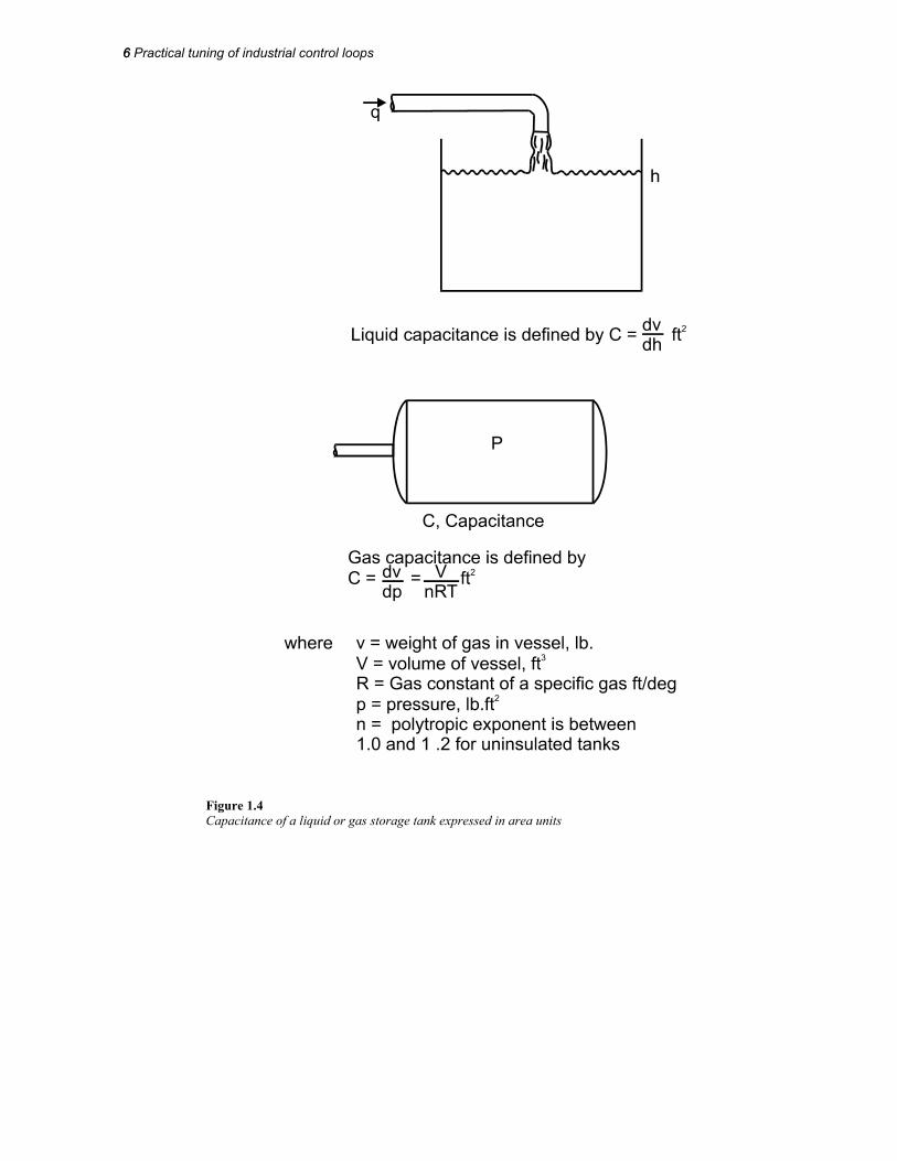
The capacitance of a liquid or gas storage tank is expressed in area units. These processes are illustrated in Figure 1.4. The gas capacitance of a tank is constant and is analogous to electrical capacitance.

The liquid capacitance equals the cross-sectional area of the tank at the liquid surface; if this is constant then the capacitance is also constant at any head.

6 Practical tuning of industrial control loops

6

Figure 1.4 Capacitance of a liquid or gas storage tank expressed in area units

Introduction

7

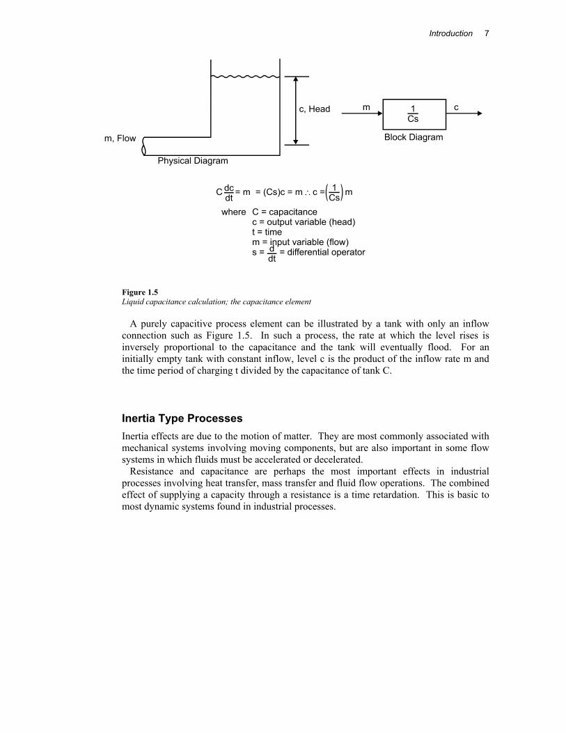
Figure 1.5 Liquid capacitance calculation; the capacitance element

A purely capacitive process element can be illustrated by a tank with only an inflow connection such as Figure 1.5. In such a process, the rate at which the level rises is inversely proportional to the capacitance and the tank will eventually flood. For an initially empty tank with constant inflow, level c is the product of the inflow rate m and the time period of charging t divided by the capacitance of tank C.

Inertia Type Processes Inertia effects are due to the motion of matter. They are most commonly associated with mechanical systems involving moving components, but are also important in some flow systems in which fluids must be accelerated or decelerated.

Resistance and capacitance are perhaps the most important effects in industrial processes involving heat transfer, mass transfer and fluid flow operations. The combined effect of supplying a capacity through a resistance is a time retardation. This is basic to most dynamic systems found in industrial processes.

8 Practical tuning of industrial control loops

8

Figure 1.6 Resistance and capacitance effects in a water heater

As a result of this time retardation, an instantaneous change in the input to the system will not result in an instantaneous change in the output. Rather, the response will be slow, requiring a finite period of time to attain a new equilibrium.

1.3 Process time constants Combining a capacitance type process element, such as a tank, and a resistance type process element, such as a valve, results in a single time constant process. In a mathematical sense, the time constant is the future time necessary to experience 63.2% of the change remaining to occur, at any moment in the process.

The time constant is a measure of the rapidity of the response of the process. It can be characterized in terms of the capacitance and resistance (or conductance) of the process.

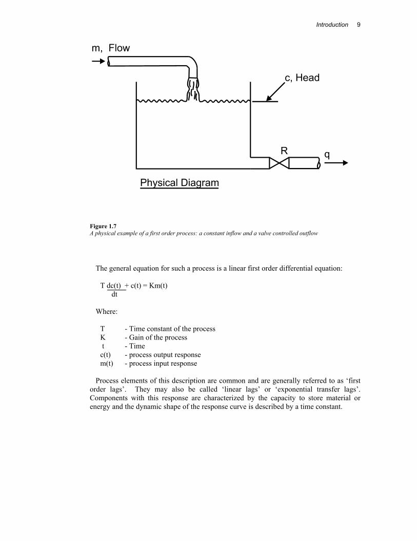
First order response In the basic case of a first order response, the maximum rate of change of output occurs immediately after a step change in input. 63.2% of the total response is attained after one time constant. If the system continued to change at its initial speed of response, the maximum response rate, it would reach 100% of the output change in one time constant. A physical example of a first order process is an initially empty tank with a constant inflow and a valve controlled outflow.

Introduction

9

Figure 1.7 A physical example of a first order process: a constant inflow and a valve controlled outflow

The general equation for such a process is a linear first order differential equation: T dc(t) + c(t) = Km(t) dt

Where: T - Time constant of the process K - Gain of the process t - Time c(t) - process output response m(t) - process input response

Process elements of this description are common and are generally referred to as ‘first order lags’. They may also be called ‘linear lags’ or ‘exponential transfer lags’. Components with this response are characterized by the capacity to store material or energy and the dynamic shape of the response curve is described by a time constant.

10 Practical tuning of industrial control loops

10

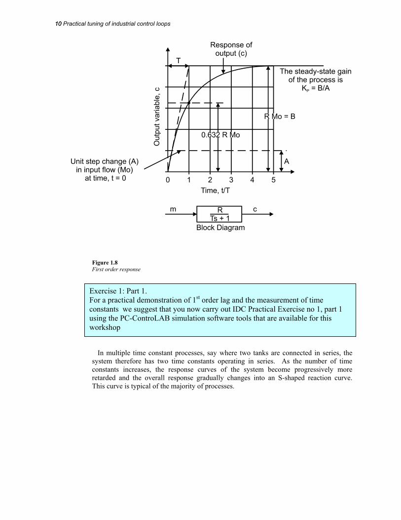
Figure 1.8 First order response

In multiple time constant processes, say where two tanks are connected in series, the

system therefore has two time constants operating in series. As the number of time constants increases, the response curves of the system become progressively more retarded and the overall response gradually changes into an S-shaped reaction curve. This curve is typical of the majority of processes.

Exercise 1: Part 1. For a practical demonstration of 1st order lag and the measurement of time constants we suggest that you now carry out IDC Practical Exercise no 1, part 1 using the PC-ControLAB simulation software tools that are available for this workshop

Introduction

11

Second order response Second order processes result in a more complicated response curve. This is due to inertia effects and interactions between first order resistance and capacitance elements. They are described by the second order differential equation:

d2 c(t) + 2xwn d c(t) +w2n c(t) = Kw2nr(t)

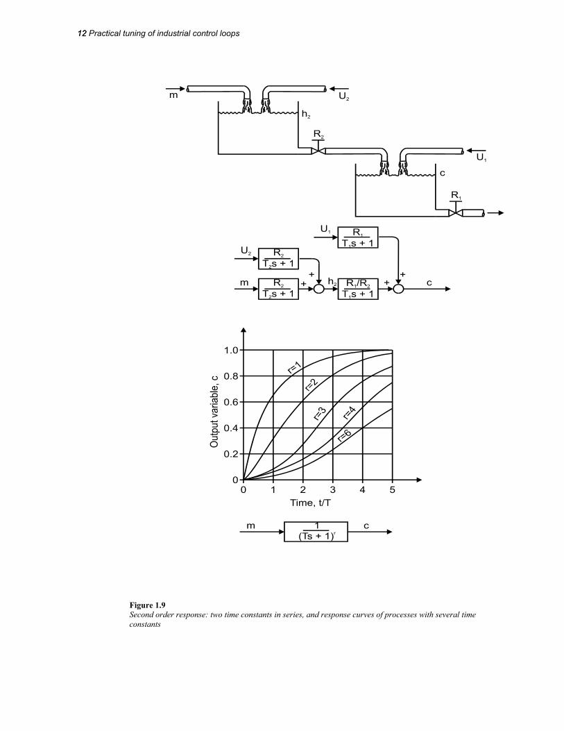
dt2 dt Where, wn - natural frequency of the system x - Damping ratio of the system K - System gain t - Time r(t) - input response of the system c(t) - output response of the system The solutions to the equation for a step change in r(t) with all initial conditions zero can

be any one of a family of curves shown in Figure 1.9. There are three possible cases in the solution, depending on the value of the damping ratio:

x < 1.0, the system is underdamped and overshoots the steady-state value. If x < 0.707, the system will oscillate about the final steady-state value. x > 1.0, the system is overdamped and will not oscillate or overshoot the final steady-

state value. x = 1.0, the system is critically damped. In this state it yields the fastest response

without overshoot or oscillation. The natural frequency term wn is related to the speed of the response for a particular

value of x. It is defined in terms of the 'perfect' or 'frictionless' situation where x = 0.0. A large frequency tends to squeeze the response and a small frequency to stretch it.

12 Practical tuning of industrial control loops

12

Figure 1.9 Second order response: two time constants in series, and response curves of processes with several time constants

Introduction

13

High Order Response Time delays can be used to approximate high-order model dynamics. Any process that consists of a large number of process units connected in series can be represented by a high order response. This transfer function could represent a series of first order transfer functions. In practice, the mathematical analysis of uncontrolled processes containing time delays is relatively simple but a time delay or a set of time delays, within a feedback loop tends to lend itself to very complex mathematics.

In general, the presence of time delays in control systems reduces the effectiveness of the controller. In well-designed systems the time delays (deadtimes) should be kept to the minimum.

1.4 Basic definitions and terms used in process control As we will see in the later chapters, two of the most important signals used in process control are called PROCESS VARIABLE or PV. and the MANIPULATED VARIABLE or MV.

In industrial process control, the PROCESS VARIABLE or PV is measured by an instrument in the field and acts as an input to a controller, which takes action based on the value of it. Alternatively the PV can be an input to computer based hardware system and its value displayed in some manner so that the operator can perform manual control and supervision.

The variable to be manipulated, in order to have control over the PV, is called the MANIPULATED VARIABLE or MV. If we control a particular flow for instance, we manipulate a valve to control the flow. Here, the valve position is called the MANIPULATED VARIABLE and the measured flow becomes the PROCESS VARIABLE.

In the case of a simple automatic controller, the Controller OUTPUT Signal (OP) drives the Manipulated Variable. In more complex automatic control systems, a controller output signal may not always drive a Manipulated Variable in the field. In practice, the term Manipulated Variable is rarely used. Most people involved in process control refer to the OP (output) of a controller and it is assumed that one knows the purpose of it.

The ideal value of the PV is often called TARGET VALUE. In the case of an automatic control, the term SET POINT VALUE is preferred.

1.5 Types or modes of operation of available control systems There are five basic forms of control available in Process Control. These are:

• On-Off • Modulating • Open Loop • Feed Forward • Closed loop

14 Practical tuning of industrial control loops

14

On-Off control The most basic control concept is the On-Off control, as found in a household iron. This is a very crude form of control, which nevertheless should be considered as a cheap and effective means of control if a fairly large fluctuation of the PV (process variable) is acceptable.

The wear and tear of the controlling element (such as actuator, solenoid valve etc) needs special consideration. As the bandwidth of fluctuation of a PV is increased, the frequency of switching (and thus wear and tear) of the controlling element decreases.

Modulating control If the output of a controller can move through a range of values, we have modulating control. It is understood that modulating control takes place within a defined operating range (with an upper and lower limit) only.

Modulating control can be used in both open and closed loop control systems.

Open loop control We have open loop control if the control action (controller output signal OP) is not a function of the PV (process variable) or load changes. The open loop control does not self-correct when the PVs drift.

Feed forward control Very often it is a form of control based on measured disturbances (feed forward control). It is a form of open loop control, as the PV is not used in the control action.

Figure 1.10 The feedforward control loop

Introduction

15

Feedforward is a more direct form of control than finding the correct value of the manipulated variable (MV) by trial and error as occurs in feedback control. In feedforward the major process variables are fed into a model to calculate the manipulated variable (MV) required to control at setpoint (SP).

Figure 1.10 shows a block diagram of a feedforward control loop. The PV (controlled variable c) is a result of the control action.

In practice, feedforward control is used in combination with feedback or closed loop control. In hybrid feedforward control, the imperfect feedforward control corrects up to 90% of the upsets, leaving the feedback system to correct the 10% bias left by the feedforward component.

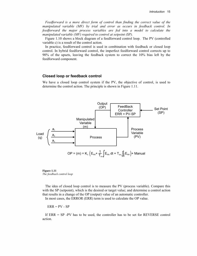
Closed loop or feedback control We have a closed loop control system if the PV, the objective of control, is used to determine the control action. The principle is shown in Figure 1.11.

Figure 1.11 The feedback control loop

The idea of closed loop control is to measure the PV (process variable). Compare this

with the SP (setpoint), which is the desired or target value; and determine a control action that results in a change of the OP (output) value of an automatic controller.

In most cases, the ERROR (ERR) term is used to calculate the OP value. ERR = PV - SP If ERR = SP -PV has to be used, the controller has to be set for REVERSE control

action.

16 Practical tuning of industrial control loops

16

1.6 Closed loop controller and process gain calculations Within this closed loop form of control there are two functional gain blocks, one being in the controller and the other in the process being controlled. The LOOPGAIN (KLOOP) is the product of the CONTROLLER GAIN (KC) and the PROCESS GAIN (KP).

LOOPGAIN (KLOOP) = KC × KP E

PVMVPVX

EMV

ΔΔ

=ΔΔ

ΔΔ

=

Where:

Process gain ( KP )MVPV

ΔΔ

=

and

Controller gain ( KC ) EMVΔΔ

=

As the total constituent parts of the entire loop consist of a minimum of 4 functional

items; the process gain ( KP )MVPV

ΔΔ

=

Controller gain ( KC ) EMVΔΔ

=

the measuring transducer or sensor gain, KS and finally the valve gain KV. The total

loop gain is the product of these four operational blocks. For ¼ damping, the ideal response where each oscillation has a ¼ of the amplitude of

the previous cycle then:

KLOOP = ( KC × KP ) = (E

PVMVPVX

EMV

ΔΔ

=ΔΔ

ΔΔ

) x KS x KV = 0.5

1.7 Proportional, integral and derivative control modes Most closed loop controllers are capable of controlling with three control modes that can be used separately or together

• Proportional control (P) • Integral, or reset control (I) • Derivative, or rate control (D)

The purpose of each of these control modes is as follows: Proportional control... This is the main and principal method of control. It calculates a control action

proportional to the ERROR (ERR). Proportional control cannot eliminate the ERROR completely.

Integral control ... (reset)

Introduction

17

This is the means to eliminate completely the remaining ERROR or OFFSET value, left from the proportional action. This may result in reduced stability in the control action.

Derivative control ... (rate) This is sometimes added to introduce dynamic stability to the control LOOP. Note: The terms RESET for integral and RATE for derivative control actions are seldom used

nowadays.

Derivative control has no functionality on its own.

The only combinations of the P, I and D modes are: • P For use as a basic controller • PI Where the offset caused by the P mode is removed • PID To remove instability problems that can occur in PI mode • PD Used in cascade control; a special application • I Used in the primary controller of cascaded systems

1.8 An introduction to cascade control Controllers are said to be "in cascade" when the output of the first or primary controller is used to manipulate the setpoint of another or secondary controller. When two or more controllers are cascaded, each will have its own measurement input or PV but only the primary controller can have an independent setpoint (SP) and only the secondary, or the most down-stream controller has an output to the process.

Cascade control is of great value where high performance is mandatory in the face of random disturbances, or where the secondary part of a process contains an undue amount of phase shift. Cascade control is one of the successful methods for improving the control performance and reducing the maximum deviation and integral error for disturbance responses. Cascade control has been used widely, as it is easy to implement and requires simple calculations.

The principal advantages of cascade control are: • The secondary controller corrects disturbances occurring in the secondary

loop before they can affect the primary, or main, variable. • The secondary controller can significantly reduce phase lag in the

secondary loop thereby improving the speed or response of the primary loop.

• Gain variations in the secondary loop are corrected within that loop. • The secondary loop enables exact manipulation of the flow of mass or

energy by the primary controller.

18 Practical tuning of industrial control loops

18

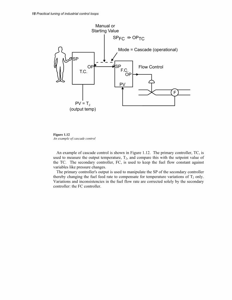
Figure 1.12 An example of cascade control

An example of cascade control is shown in Figure 1.12. The primary controller, TC, is

used to measure the output temperature, T2, and compare this with the setpoint value of the TC. The secondary controller, FC, is used to keep the fuel flow constant against variables like pressure changes.

The primary controller's output is used to manipulate the SP of the secondary controller thereby changing the fuel feed rate to compensate for temperature variations of T2 only. Variations and inconsistencies in the fuel flow rate are corrected solely by the secondary controller: the FC controller.