A Practical, Real-Time Auto-Tuning Framework for … · Technical Report FSL-18-01 April 2018....

A Practical, Real-Time Auto-Tuning Framework forStorage Systems

A Dissertation Proposal Presented

by

Zhen Cao

to

The Graduate School

in Partial Fulfillment of the

Requirements

for the Degree of

Doctor of Philosophy

in

Computer Science

Stony Brook University

Technical Report FSL-18-01

April 2018

Abstract

A Practical, Real-Time Auto-Tuning Framework for Storage Systems

by

Zhen Cao

Doctor of Philosophy Candidatein

Computer Science

Stony Brook University2018

Storage systems come with a large number of configurable parameters that control their be-havior. Tuning such parameters can provide significant gains in performance, but is challengingbecause of huge parameter spaces and complex, non-linear system behavior. Auto-tuning withblack-box optimization have shown some promising results in recent years, thanks to its oblivious-ness to systems’ internals.

However, previous work all applied only one or few optimization methods, and did not sys-tematically evaluate them. Therefore, in this thesis proposal, we first apply and then perform com-parative analysis of multiple black-box optimization techniques on storage systems from variousaspects such as their ability to find near-optimal configurations, convergence time, and instanta-neous system throughput during auto-tuning, etc. We also provide insights into the efficacy ofthese automated black-box optimization methods from a system’s perspective.

During our auto-tuning experiments, we noticed that sometimes multiple runs of the sameworkload—in a carefully controlled environment—produced widely different performance results.So next, we undertook a study to characterize the amount of variability in modern storage systems.We analyzed these variations and found that there was no single root cause: it often changed withthe workload, hardware, or software configuration in the storage system. In several of those caseswe were able to fix the cause of variation and reduce it to acceptable levels.

Despite some promising early results, we believe several critical features are still missing fromtraditional black-box optimization methods. Therefore, we propose to investigate and design amore intelligent and practical framework for auto-tuning storage systems in real-time. We definestopping and restarting criteria to stop auto-tuning when “good enough” configurations are foundand restart it in response to environment changes. We add a workload modeler to characterizethe running workload. Initialization methods will be studied as well, which showed significantimpact on the overall efficacy of auto-tuning in our preliminary results. Our framework includes aweighted penalty function, to account for costly configuration changes. We also plan to investigatehow Machine Learning (ML) techniques can help on various aspects of our auto-tuning framework(e.g., identify unimportant parameters and eliminate them from the search space).

It is our thesis that real-time auto-tuning storage systems is important, promising, and feasiblewith a carefully designed framework to include missing yet critical features. This can improvesystems’ performance efficiency, and save energy and human resources in the long term.

ii

Contents

List of Figures v

List of Tables vii

Acknowledgments ix

1 Introduction 1

2 Background 42.1 Problem Statement . . . . . . . . . . . . . . . . . . . . . . . . . . . . . . . . . . 42.2 Black-box Optimization . . . . . . . . . . . . . . . . . . . . . . . . . . . . . . . . 72.3 Machine Learning . . . . . . . . . . . . . . . . . . . . . . . . . . . . . . . . . . . 82.4 Unified Framework . . . . . . . . . . . . . . . . . . . . . . . . . . . . . . . . . . 9

3 Related Work 113.1 Auto-tuning in Computer Systems . . . . . . . . . . . . . . . . . . . . . . . . . . 113.2 Hyper-parameter tuning . . . . . . . . . . . . . . . . . . . . . . . . . . . . . . . . 123.3 Workload Modeling . . . . . . . . . . . . . . . . . . . . . . . . . . . . . . . . . . 12

4 Experimental Settings 134.1 Hardware . . . . . . . . . . . . . . . . . . . . . . . . . . . . . . . . . . . . . . . 134.2 Workload . . . . . . . . . . . . . . . . . . . . . . . . . . . . . . . . . . . . . . . 134.3 Parameter Space . . . . . . . . . . . . . . . . . . . . . . . . . . . . . . . . . . . . 154.4 Experiments and Implementations . . . . . . . . . . . . . . . . . . . . . . . . . . 16

5 Towards Better Understanding of Black-box Auto-Tuning: A Comparative Analysisfor Storage Systems 185.1 Overview of Datasets . . . . . . . . . . . . . . . . . . . . . . . . . . . . . . . . . 195.2 Comparative Analysis . . . . . . . . . . . . . . . . . . . . . . . . . . . . . . . . . 205.3 Impact of Hyper-Parameters . . . . . . . . . . . . . . . . . . . . . . . . . . . . . 245.4 Peering into the Black Box . . . . . . . . . . . . . . . . . . . . . . . . . . . . . . 255.5 Limitations . . . . . . . . . . . . . . . . . . . . . . . . . . . . . . . . . . . . . . 28

6 On the Performance Variation in Modern Storage Systems 296.1 Motivations . . . . . . . . . . . . . . . . . . . . . . . . . . . . . . . . . . . . . . 296.2 Background . . . . . . . . . . . . . . . . . . . . . . . . . . . . . . . . . . . . . . 31

iii

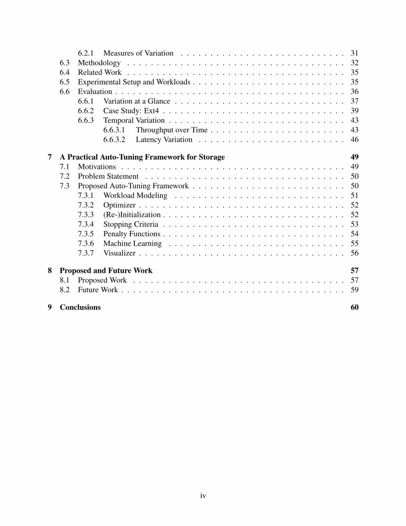
6.2.1 Measures of Variation . . . . . . . . . . . . . . . . . . . . . . . . . . . . 316.3 Methodology . . . . . . . . . . . . . . . . . . . . . . . . . . . . . . . . . . . . . 326.4 Related Work . . . . . . . . . . . . . . . . . . . . . . . . . . . . . . . . . . . . . 356.5 Experimental Setup and Workloads . . . . . . . . . . . . . . . . . . . . . . . . . . 356.6 Evaluation . . . . . . . . . . . . . . . . . . . . . . . . . . . . . . . . . . . . . . . 36

6.6.1 Variation at a Glance . . . . . . . . . . . . . . . . . . . . . . . . . . . . . 376.6.2 Case Study: Ext4 . . . . . . . . . . . . . . . . . . . . . . . . . . . . . . . 396.6.3 Temporal Variation . . . . . . . . . . . . . . . . . . . . . . . . . . . . . . 43

6.6.3.1 Throughput over Time . . . . . . . . . . . . . . . . . . . . . . . 436.6.3.2 Latency Variation . . . . . . . . . . . . . . . . . . . . . . . . . 46

7 A Practical Auto-Tuning Framework for Storage 497.1 Motivations . . . . . . . . . . . . . . . . . . . . . . . . . . . . . . . . . . . . . . 497.2 Problem Statement . . . . . . . . . . . . . . . . . . . . . . . . . . . . . . . . . . 507.3 Proposed Auto-Tuning Framework . . . . . . . . . . . . . . . . . . . . . . . . . . 50

7.3.1 Workload Modeling . . . . . . . . . . . . . . . . . . . . . . . . . . . . . 517.3.2 Optimizer . . . . . . . . . . . . . . . . . . . . . . . . . . . . . . . . . . . 527.3.3 (Re-)Initialization . . . . . . . . . . . . . . . . . . . . . . . . . . . . . . . 527.3.4 Stopping Criteria . . . . . . . . . . . . . . . . . . . . . . . . . . . . . . . 537.3.5 Penalty Functions . . . . . . . . . . . . . . . . . . . . . . . . . . . . . . . 547.3.6 Machine Learning . . . . . . . . . . . . . . . . . . . . . . . . . . . . . . 557.3.7 Visualizer . . . . . . . . . . . . . . . . . . . . . . . . . . . . . . . . . . . 56

8 Proposed and Future Work 578.1 Proposed Work . . . . . . . . . . . . . . . . . . . . . . . . . . . . . . . . . . . . 578.2 Future Work . . . . . . . . . . . . . . . . . . . . . . . . . . . . . . . . . . . . . . 59

9 Conclusions 60

iv

List of Figures

2.1 Storage systems are non-linear . . . . . . . . . . . . . . . . . . . . . . . . . . . . 52.2 Evaluation results depend on workloads . . . . . . . . . . . . . . . . . . . . . . . 62.3 Crossover and mutation in a Genetic Algorithm . . . . . . . . . . . . . . . . . . . 8

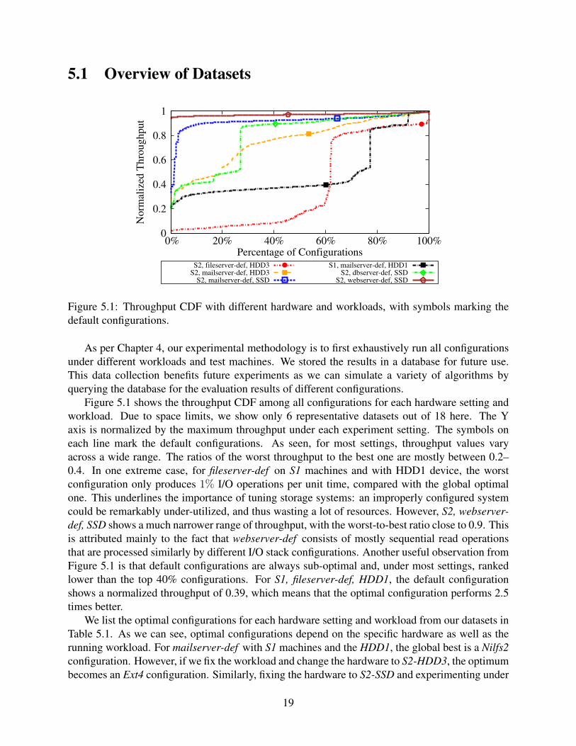
5.1 Throughput CDF with different hardware and workloads, with symbols markingthe default configurations. . . . . . . . . . . . . . . . . . . . . . . . . . . . . . . 19

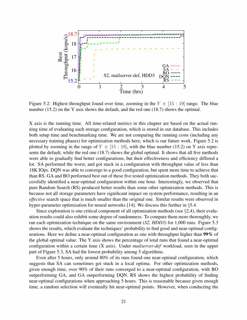
5.2 Highest throughput found over time, zooming in the Y ∈ [15 : 19] range. The bluenumber (15.2) on the Y axis shows the default, and the red one (18.7) shows theoptimal. . . . . . . . . . . . . . . . . . . . . . . . . . . . . . . . . . . . . . . . . 21

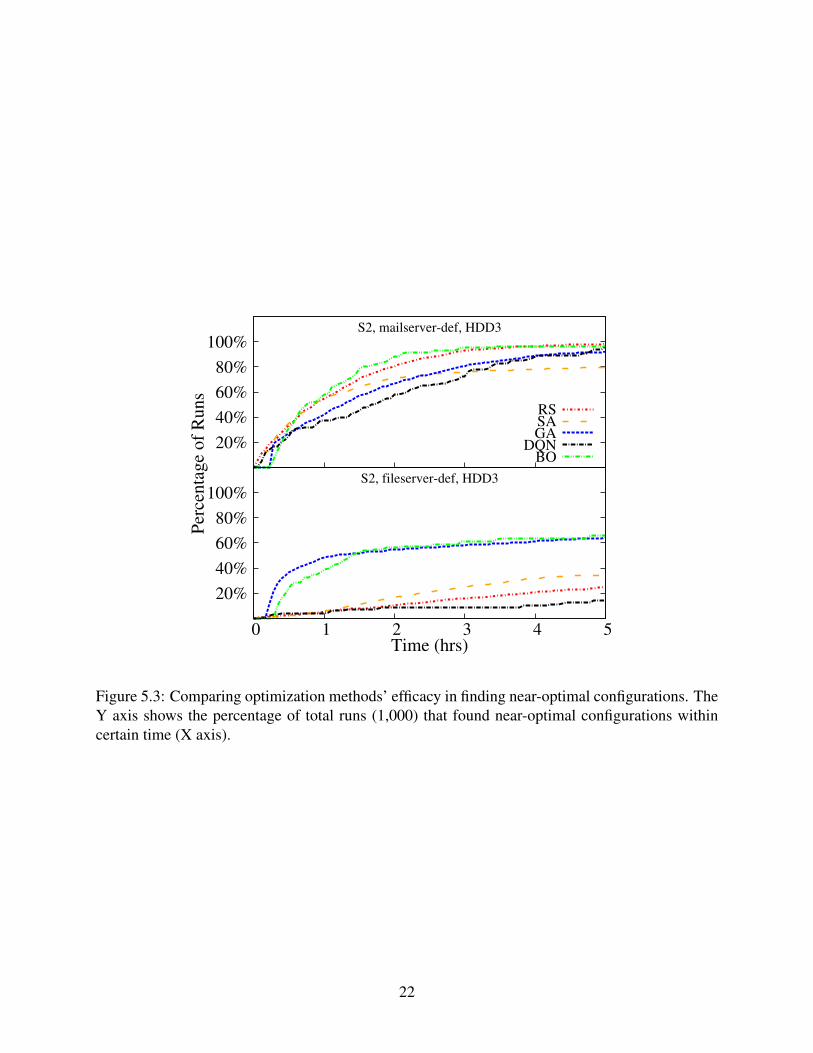
5.3 Comparing optimization methods’ efficacy in finding near-optimal configurations.The Y axis shows the percentage of total runs (1,000) that found near-optimalconfigurations within certain time (X axis). . . . . . . . . . . . . . . . . . . . . . 22

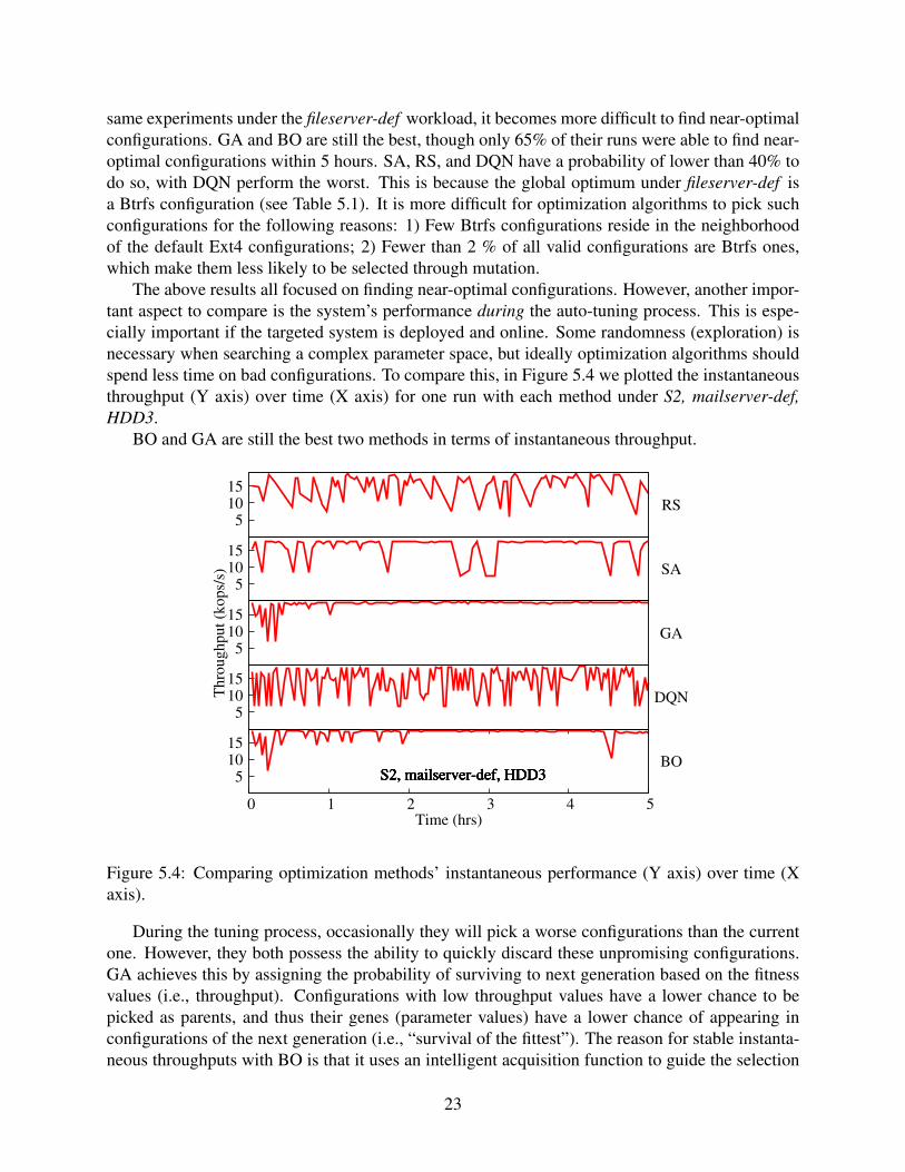
5.4 Comparing optimization methods’ instantaneous performance (Y axis) over time(X axis). . . . . . . . . . . . . . . . . . . . . . . . . . . . . . . . . . . . . . . . . 23

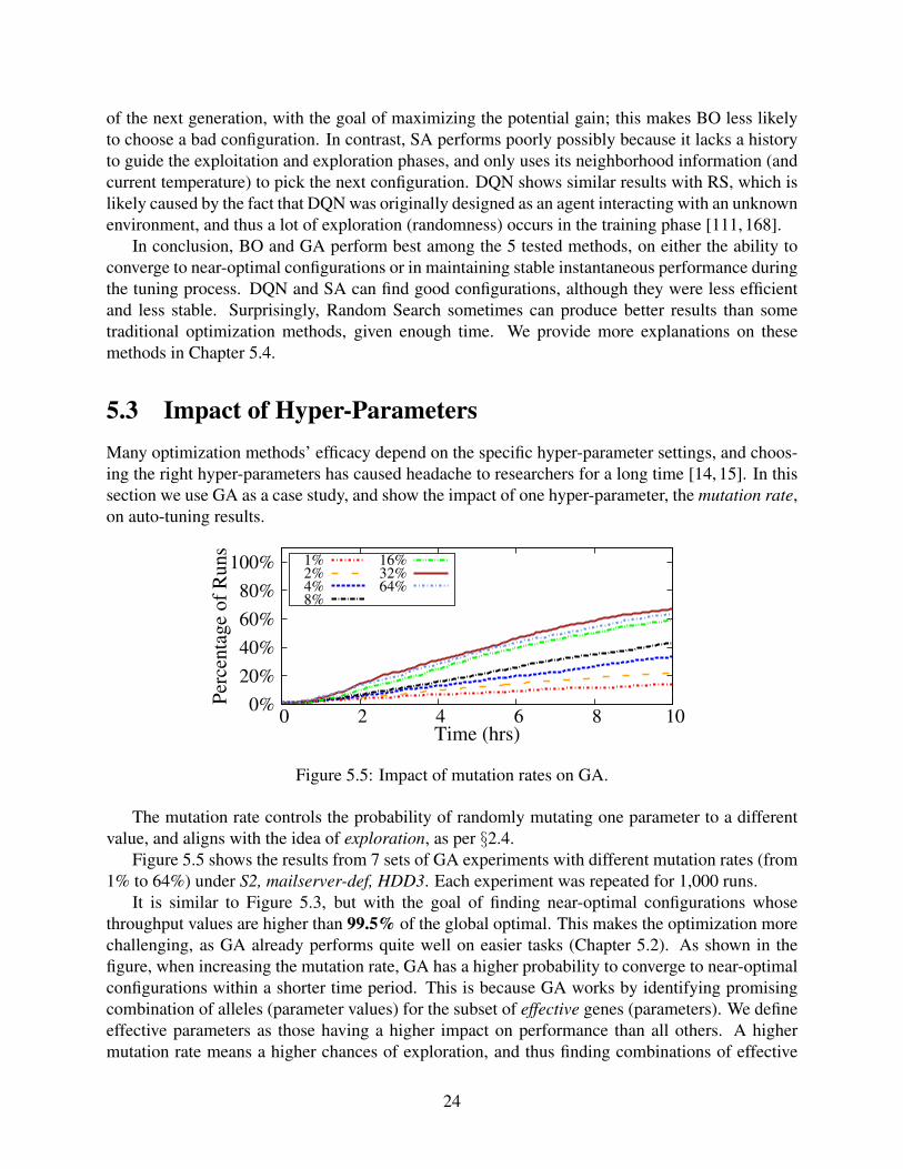
5.5 Impact of mutation rates on GA. . . . . . . . . . . . . . . . . . . . . . . . . . . . 245.6 Number of alleles (parameter values) in the first 10 generations from one GA ex-

periment run, with more frequent ones colored with darker colors. . . . . . . . . . 255.7 Scatter plot for all Ext3-SSD configurations under fileserver-def workload, with

one dot corresponding to one configuration. . . . . . . . . . . . . . . . . . . . . . 26

6.1 Cumulative throughput over time for one Ext4 configuration under multiple work-loads. Each workload ran for 7,200s; only the first 3,000s are plotted. . . . . . . . 36

6.2 Overview of performance and its variation with different storage configurations un-der three workloads: (a) maileserver-heavy, (b) fileserver-heavy, and (c) webserver-heavy. The X axis represents the mean of throughput over 10 runs; the Y axisshows the relative range of cumulative throughput. Ext4 configurations are repre-sented with squares, XFS with circles, and Btrfs with triangles. HDD configura-tions are shown with filled symbols, and SSDs with hollow ones. . . . . . . . . . . 37

6.3 Storage system performance variation with 20 sampled Ext4-HDD configurationsunder three workloads. The range is computed among 10 experiment runs, and isrepresented as bars corresponding to the Y1 (left) axis. The mean of throughputamong the 10 runs is shown with symbols (squares, circles, and triangles), andcorresponds to the Y2 (right) axis. The X axis represents configurations formattedby 〈block size - inode size - journal - atime - I/O scheduler - device〉. . . . . . . . . 38

v

6.4 Performance variation for 2 Ext4-HDD configurations with several diagnoses. Eachexperiment is shown as one box, representing a throughput distribution for 10 iden-tical runs. The top border line of each box marks the 1st quartile; the bottom bor-der marks the 3rd quartile; the line in the middle is the median throughput; and thewhiskers mark maximum and minimum values. The dots to the right of each boxshow the exact throughputs of all 10 runs. The percentage numbers below eachbox are the relative range values. The bottom label shows configuration details foreach figure. . . . . . . . . . . . . . . . . . . . . . . . . . . . . . . . . . . . . . . 39

6.5 Performance variation for Ext4-HDD configuration under the Fileserver workloadwith different partition sizes from inner tracks of disks . . . . . . . . . . . . . . . 41

6.6 Physical blocks of allocated files in Ext4 under the Fileserver workload. The Xaxis represents the physical block number of each file in the dataset. Since the File-server workload consists of small files, and one extent per file, we use the startingblock number for each file here. The Y axis is the final cumulative throughput foreach experiment run. Note that the Y axis does not start from 0. Lines markedwith solid circles are experiment runs with the default setting; lines with trianglesrepresent experiment runs where we set the field s hash seed in Ext4s’s superblockto null. . . . . . . . . . . . . . . . . . . . . . . . . . . . . . . . . . . . . . . . . . 42

6.7 Throughput-120 over time for Btrfs, XFS, and Ext4 HDD configurations under theFileserver workload. Each configuration was evaluated for 10 runs. Two lines wereplotted connecting maximum and minimum throughput values among 10 runs. Wefill in colors between two lines, green for Btrfs, red for Ext4, and blue for XFS. Wealso plotted the average Throughput-120 among 10 runs as a line running throughthe band. The maximum relative range values of Throughput-120 for Ext4, Btrfs,and XFS are 43%, 23%, and 65%, while the minimum values are 14%, 2%, and7%, respectively. . . . . . . . . . . . . . . . . . . . . . . . . . . . . . . . . . . . 43

6.8 CDFs for relative range of throughput under Fileserver workload with differentwindow sizes. For window size N, we calculated the relative range values ofthroughput for all configurations within each file system type, and then plottedthe corresponding CDF. . . . . . . . . . . . . . . . . . . . . . . . . . . . . . . . 45

6.9 Normalized instantaneous throughput (Throughput-10) over time for experimentswith various workloads, file systems, and devices. The Y axis shows the normal-ized values divided by the maximum instantaneous throughput through the exper-iment. Only the first 500s are presented for brevity. . . . . . . . . . . . . . . . . . 46

6.10 Latency CDF of one Ext4-HDD configuration under Fileserver workload. . . . . . 476.11 Pearson Correlation Coefficient (PCC) between throughput range and operation

types, for three workloads and three file systems. The horizontal dashed red line atY=0.7 marks the point above which a strong correlation is often considered to exist. 48

7.1 Auto-tuning Framework . . . . . . . . . . . . . . . . . . . . . . . . . . . . . . . 517.2 Work flow for an enhanced Optimizer (GA). . . . . . . . . . . . . . . . . . . . . 527.3 Comparison of different initialization methods. . . . . . . . . . . . . . . . . . . . 537.4 Time window based stopping criteria. . . . . . . . . . . . . . . . . . . . . . . . . 54

vi

8.1 Auto-tuning Framework. Components are re-colored based on our project time-line. We plan to completely finish work colored by green; partially finish workcolored by yellow. Components colored with red are left for future work beyondthis thesis. . . . . . . . . . . . . . . . . . . . . . . . . . . . . . . . . . . . . . . 58

8.2 Work flow for an enhanced Optimizer (GA). Components are re-colored based onour project timeline. We plan to completely finish work colored by green; partiallyfinish work colored by yellow. Components colored with red are left for futurework beyond this thesis. . . . . . . . . . . . . . . . . . . . . . . . . . . . . . . . 59

vii

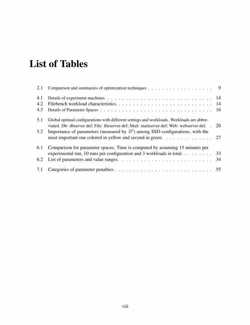
List of Tables

2.1 Comparison and summaries of optimization techniques . . . . . . . . . . . . . . . . . . 9

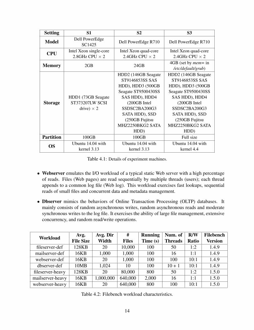
4.1 Details of experiment machines. . . . . . . . . . . . . . . . . . . . . . . . . . . . . . 144.2 Filebench workload characteristics. . . . . . . . . . . . . . . . . . . . . . . . . . . 144.3 Details of Parameter Spaces . . . . . . . . . . . . . . . . . . . . . . . . . . . . . . . 16

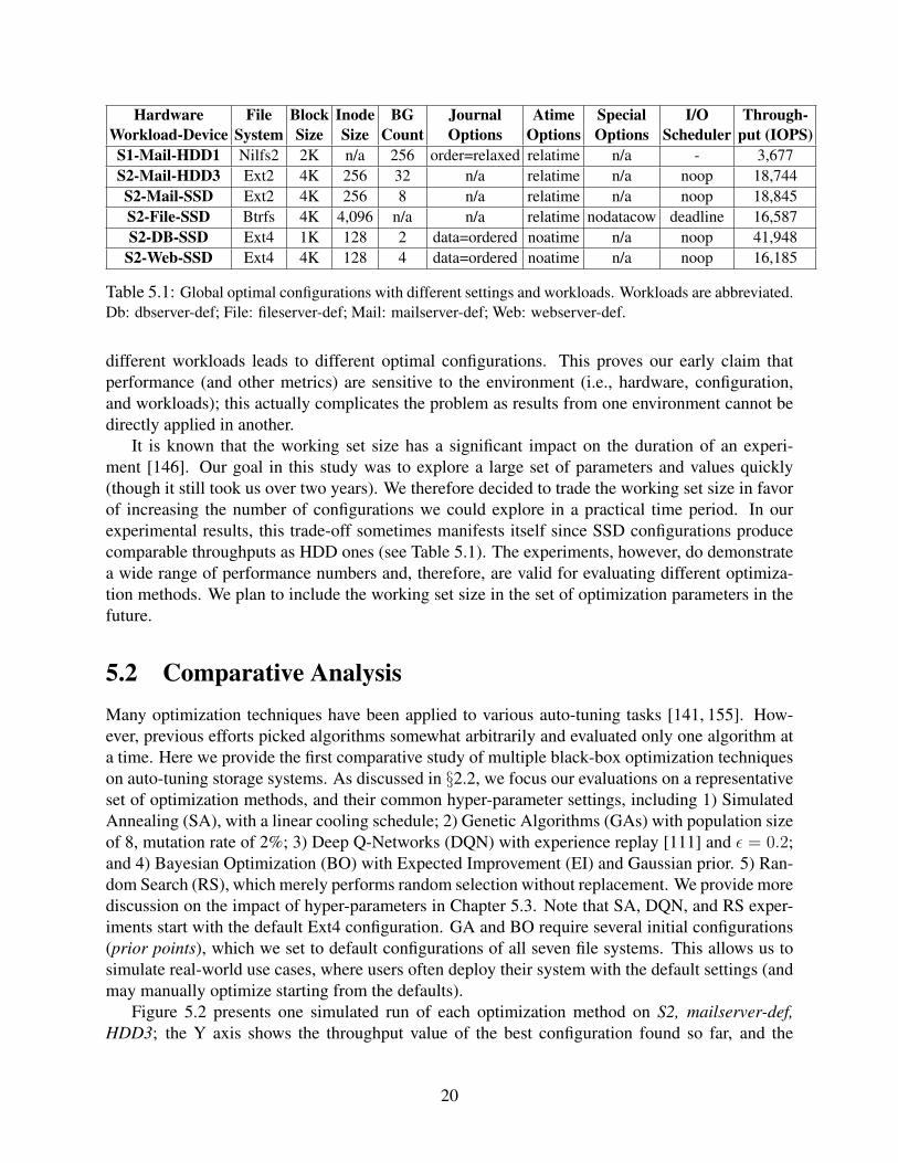
5.1 Global optimal configurations with different settings and workloads. Workloads are abbre-viated. Db: dbserver-def; File: fileserver-def; Mail: mailserver-def; Web: webserver-def. . 20

5.2 Importance of parameters (measured by R2) among SSD configurations, with themost important one colored in yellow and second in green. . . . . . . . . . . . . . 27

6.1 Comparison for parameter spaces. Time is computed by assuming 15 minutes perexperimental run, 10 runs per configuration and 3 workloads in total. . . . . . . . . 33

6.2 List of parameters and value ranges. . . . . . . . . . . . . . . . . . . . . . . . . . 34

7.1 Categories of parameter penalties . . . . . . . . . . . . . . . . . . . . . . . . . . . 55

viii

Acknowledgments

Chapter 1

Introduction

Storage is a critical element of computer systems and key to data-intensive applications. Storagesystems come with a vast number of configurable parameters that control a system’s behavior. Ext4alone has around 60 parameters with whopping 1037 unique combinations of values. Default pa-rameter settings provided by vendors are often suboptimal for a specific user deployment; previousresearch showed that tuning even a small subset of parameters can improve power and performanceefficiency of storage systems by as much as 9× [132].

Traditionally, system administrators pick parameter settings based on their expertise and ex-perience. Due to the increased complexity of storage systems, however, manual tuning becomesintractable, error-prone, and has a low chance of finding an optimal configuration. A myriad of filesystems with diverse goals and designs have been developed [47, 83, 87, 124, 144]. Newer typesof devices (SSDs [64, 108], SMR drives [2, 3], PCM [81, 163]) and more layers (LVM, RAID)are added. Storage systems expand from one or few identical nodes to hundreds of highly het-erogeneous environments [55, 129]. Tuning results from one workload are often inapplicable inanother [24, 155]. Furthermore, the composition of hardware and workload in a modern environ-ment changes at a fast pace that prohibits timely manual tuning.

In recent years, several attempts were made to automate the tuning of computer systems ingeneral and storage systems in particular [141, 155]. Black-box auto-tuning is an especially popu-lar approach thanks to its obliviousness to system’s internals [170]. The basic mechanism behindblack-box auto-tuning is to iteratively try different configurations, measure an objective function’svalue—and based on the previously learned information—select the next configurations to try.For storage systems, objective functions can be throughput, I/O latency, energy consumption, pur-chase cost, or even a formula combining multiple metrics [97, 141]. Many black-box auto-tuningalgorithms exist and some were applied to systems. Genetic Algorithms (GA) were applied tooptimize the I/O performance of HDF5-based applications [12]. Bayesian Optimization (BO) wasused to find a near-optimal configuration for Cloud VMs [5]. Other methods include Evolution-ary Strategies [126], Smart Hill-Climbing [164], and Simulated Annealing [42]. Although thesemethods were originally proposed in different scientific disciplines, they all maintain a trade-offamong three behavioral dimensions: (1) Exploration: how much the technique searches the spacerandomly. (2) Exploitation: how much the technique leverages the “neighborhood” of the currentcandidate or previous search history to find even better configurations. (3) History: how much datafrom previous evaluations is kept and utilized in the overall search process. For this dissertation,we propose to investigate and design a general framework based on black-box optimization, which

1

can efficiently auto-tune storage systems in real-time.To demonstrate black-box optimization’s ability to find optimal (or at least near-optimal) stor-

age configurations, we started by exhaustively evaluating several storage systems under four work-loads on two servers with different hardware and storage devices; the largest system consisted of6,222 unique configurations. Over a period of 2+ years, we executed 450,000+ experimental runs,with 18 different combination of workload and hardware settings. We stored all data points in arelational database for query convenience, including hardware and workload details, throughput,energy consumption, running time, etc. In this thesis proposal, we mainly focused on optimizingfor 0throughput, but our methodology and observations are applicable to other metrics as well. Weplan to release our dataset publicly to facilitate more research into auto-tuning and better under-standing of storage systems.

Despite some appealing results in auto-tuning, there is no deep understanding how exactlythese black-box optimization methods work, their efficacy and efficiency, and which methods aremore suitable for which problems. Previous works picked algorithms somewhat arbitrarily andevaluated only one algorithm at a time. Therefore, in this proposal, for the first time and to thebest of our knowledge, we apply and analytically compare multiple black-box optimization tech-niques on storage systems. We applied several popular techniques to the collected dataset to findoptimal configurations under various hardware and workload settings: Simulated Annealing (SA),Genetic Algorithms (GA), Bayesian Optimization (BO), and Deep Q-Networks (DQN). We alsotried Random Search (RS) in our experiments, which showed surprisingly good results in previousresearch [15]. We compared these techniques from various aspects, such as their ability to findnear-optimal configurations, convergence time, and instantaneous system throughput during auto-tuning. For example, we found that several techniques were able to converge to good configurationsgiven enough time, but their efficacy differed a lot. GA and BO outperformed SA and DQN on ourparameter spaces, both in terms of convergence time and instantaneous throughputs. Surprisingly,RS was also able to identify good configurations, sometimes even more efficiently than sophisti-cated optimization methods. We further compared the techniques across the aforementioned threebehavioral dimensions: exploration, exploitation, and history. Based on our experimental resultsand domain expertise, we also provide explanations of efficacy of such black-box optimizationmethods from a storage perspective. We observed that certain parameters would have a greatereffect on system performance than others, and the set of dominant parameters depends on filesystems and workloads.

During our auto-tuning experiments, we noticed that sometimes multiple runs of the sameworkload—in a carefully controlled environment—produced widely different performance results.In one experiment setting, over 18% of 6,222 different storage configurations that we tried exhib-ited a standard deviation of performance larger than 5% of the mean, and a range value (maximumminus minimum performance, divided by the average) that exceeding 9%. In a few extreme cases,the standard deviation exceeded 40% even with numerous repeated experiments. This motivated usto conduct a more detailed study of storage system performance variation and seek its root causes,as performance stability is important for the success of auto-tuning and more broadly is critical inmodern storage systems. Therefore, in this proposal we conducted experiments on three local filesystems (Ext4, XFS, and Btrfs) which are used in many modern local and distributed environments.We benchmarked over 100 configurations using different workloads and repeated each experiment10 times to balance the accuracy of variation measurement with the total time taken to completethese experiments. We then characterized performance variation from several angles: throughput,

2

latency, temporally, spatially, and more. We found that performance variation depends heavily onthe specific configuration of the storage system. We then further dove into the details, analyzedand explained certain performance variations. For example, we found that unpredictable layoutsin Ext4 could cause over 16–19% of performance variation in some cases. Finally, we analyzedlatency variations from various aspects, and proposed a novel approach for quantifying the impactsof each operation type on overall performance variation.

Despite some promising preliminary results, we believe traditional black-box optimizationtechniques still lack several critical features to achieve practical, real-time auto-tuning in stor-age systems. Our own experiments demonstrate that auto-tuning sometimes can be slow in findingnear-optimal configurations, especially when the evaluation of even a single configuration takeslong time (e.g., due to slow I/O). Worse, when each experiment itself takes a long time (e.g., dueto slower I/Os), using such techniques alone can take even longer. Moreover, there is no implicitmechanism to stop the search when it reaches a sufficiently good configuration (and restart it lateron as needed); little is known on how to initialize the search and give it a good starting point; andthere is no accounting for the cost of moving from one configuration to another, which is criticallyimportant in some production settings.

Therefore, for this dissertation we propose to investigate and develop a more intelligent andpractical auto-tuning framework, intended to dynamically optimize storage systems. We are ex-ploring techniques that add vital missing features from existing optimization methods: (1) A cri-teria when the optimization algorithm should stop searching, having reached a “good enough”system configuration. (2) A similar criteria when the search algorithm should be restarted, usefulwhen the environment conditions (e.g., workload) have changed enough to take the system offof its optimal point. (3) A workload modeler, which can extract features from collected systemmetrics and characterize the running workload based on them. This is useful in determining whento restart the auto-tuning process and how to “transfer” evaluation results from one workload toanother. (4) A mechanism to pick an initial set of search space locations, as well as re-initialize thesearch space after restarting a search—which we have found to have a big impact on the efficacyof any search [23, 43]. (5) A penalty function to assign a (weighted) cost to any new configurationbased on the current system state, to account for costly configuration changes (e.g., a simple run-time changeable parameter vs. one that requires a system reboot and some downtime). We describesome preliminary results exploring these proposed ideas, and discuss how these components couldhelp us achieve the goal of auto-tuning storage systems in real-time.

The rest of this dissertation proposal is organized as follows. Chapter 2 describes challengesof auto-tuning storage systems and background knowledge on black-box optimization. Chapter 3discusses related work. We list our experimental settings in Chapter 4. In Chapter 5 we performa comparative analysis on multiple optimization methods. Chapter 6 provides our characterizationwork on performance variation in modern storage stocks. Chapter 7 discusses several missingyet important components from traditional black-box optimization. Based on it, we propose toinvestigate and design a more intelligent and practical auto-tuning framework for storage systems.Chapter 9 concludes this proposal.

3

Chapter 2

Background

In this thesis proposal we use “storage systems” to refer file systems, underlying storage hard-ware and any layers between them. Storage systems have always been a critical component ofmost computer systems, and are the foundation for many data-intensive applications. Usuallythey come with a large number of configurable options that could affect or even determine thesystems’ performance [24, 146], energy consumption [132], and other aspects [94, 141]. Herewe define a parameter as one configurable option, and a configuration as a certain combina-tion of parameter values. For example, the journal mode is one parameter for Ext4, with 3possible values: data=writeback, data=ordered, and data=journal. Two other common param-eters are block size and inode size with several possible numeric values (e.g., 4K, 8K). [jour-nal mode=“data=writeback”, block size=4K, inode size=4K] is one configuration with 3 specificparameters: journal mode, block size, and inode size. All possible configurations form a parameterspace.

When configuring storage systems, users often stick with the default configurations providedby vendors because

• it is nearly impossible to know the impact of every parameter across multiple layers; and

• vendors’ default configurations are trusted to be safe and “good enough”.

However, previous studies [132] showed that tuning even a tiny subset of parameters could improvethe performance and energy efficiency for storage systems by as much as 9×. As Moore’s lawslows down, it becomes even more important to squeeze every bit of performance out of deployedstorage systems.

The rest of this chapter is organized as follows. We first discuss the challenges of storagesystem tuning in Chapter 2.1. Then, Chapter 2.2 briefly introduces several black-box optimizationtechniques that we explore in this proposal. Chapter 2.3 discusses how Machine Learning (ML)techniques can help in auto-tuning storage systems. Chapter 2.4 provides a unified view of theseoptimization methods.

2.1 Problem StatementThe tuning task for storage systems is difficult, due to the following four challenges.

4

(1) Large parameter space Modern storage systems are fairly complex and easily come withhundreds or even thousands of tunable parameters. This makes it impossible to explore even asmall fraction of the parameter space exhaustively. Even human experts or file-system developerscannot know the exact impact of every parameter and thus have little insight into how to optimizethem. For example, Ext4 + NFS alone would result in a parameter space consisting of more than1022 unique configurations. IBM’s General Parallel File System (GPFS) [129] contains more than100 tunable parameters, and hence 1040 configurations. From the hardware perspective, which alsoconstitutes part of parameter space, SSDs [64,108,115,130], SMRs [2,3,68,92], and PCM [81,163]are gaining popularity and more layers (LVM, RAID) are added to storage systems.

(2) Discrete and non-numeric parameters Among storage system parameters, some can takea continuous spectrum of values, while many others are discrete and take only a limited set ofvalues. Some parameters do not even have numeric values (e.g., I/O scheduler name or file systemtype). These types of parameters make gradient-based information for objective functions (e.g.,linear regression) unavailable.

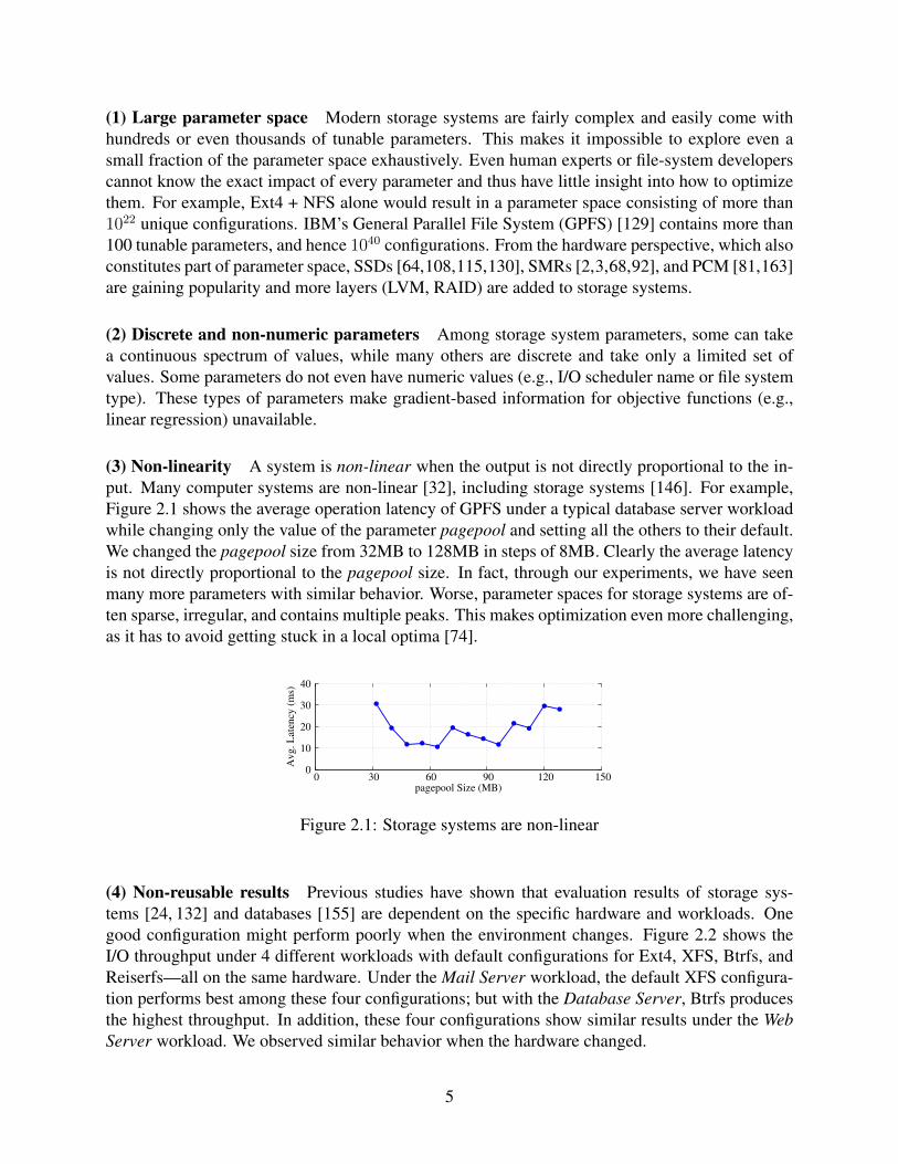
(3) Non-linearity A system is non-linear when the output is not directly proportional to the in-put. Many computer systems are non-linear [32], including storage systems [146]. For example,Figure 2.1 shows the average operation latency of GPFS under a typical database server workloadwhile changing only the value of the parameter pagepool and setting all the others to their default.We changed the pagepool size from 32MB to 128MB in steps of 8MB. Clearly the average latencyis not directly proportional to the pagepool size. In fact, through our experiments, we have seenmany more parameters with similar behavior. Worse, parameter spaces for storage systems are of-ten sparse, irregular, and contains multiple peaks. This makes optimization even more challenging,as it has to avoid getting stuck in a local optima [74].

0

10

20

30

40

0 30 60 90 120 150

Av

g.

Lat

ency

(m

s)

pagepool Size (MB)

Figure 2.1: Storage systems are non-linear

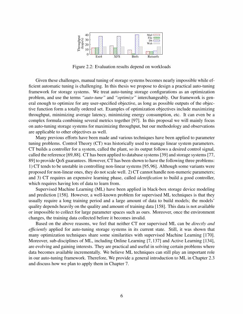
(4) Non-reusable results Previous studies have shown that evaluation results of storage sys-tems [24, 132] and databases [155] are dependent on the specific hardware and workloads. Onegood configuration might perform poorly when the environment changes. Figure 2.2 shows theI/O throughput under 4 different workloads with default configurations for Ext4, XFS, Btrfs, andReiserfs—all on the same hardware. Under the Mail Server workload, the default XFS configura-tion performs best among these four configurations; but with the Database Server, Btrfs producesthe highest throughput. In addition, these four configurations show similar results under the WebServer workload. We observed similar behavior when the hardware changed.

5

0

10

20

30

40

Ext4 XFS Btrfs Reiserfs

Thro

ughput

(kops/

s)

MailFileDb

Web

Figure 2.2: Evaluation results depend on workloads

Given these challenges, manual tuning of storage systems becomes nearly impossible while ef-ficient automatic tuning is challenging. In this thesis we propose to design a practical auto-tuningframework for storage systems. We treat auto-tuning storage configurations as an optimizationproblem, and use the terms “auto-tune” and “optimize” interchangeably. Our framework is gen-eral enough to optimize for any user-specified objective, as long as possible outputs of the objec-tive function form a totally ordered set. Examples of optimization objectives include maximizingthroughput, minimizing average latency, minimizing energy consumption, etc. It can even be acomplex formula combining several metrics together [97]. In this proposal we will mainly focuson auto-tuning storage systems for maximizing throughput, but our methodology and observationsare applicable to other objectives as well.

Many previous efforts have been made and various techniques have been applied to parametertuning problems. Control Theory (CT) was historically used to manage linear system parameters.CT builds a controller for a system, called the plant, so its output follows a desired control signal,called the reference [69,88]. CT has been applied to database systems [39] and storage systems [77,89] to provide QoS guarantees. However, CT has been shown to have the following three problems:1) CT tends to be unstable in controlling non-linear systems [95,96]. Although some variants wereproposed for non-linear ones, they do not scale well. 2) CT cannot handle non-numeric parameters;and 3) CT requires an expensive learning phase, called identification to build a good controller,which requires having lots of data to learn from.

Supervised Machine Learning (ML) have been applied in black-box storage device modelingand prediction [158]. However, a well-known problem for supervised ML techniques is that theyusually require a long training period and a large amount of data to build models; the models’quality depends heavily on the quality and amount of training data [158]. This data is not availableor impossible to collect for large parameter spaces such as ours. Moreover, once the environmentchanges, the training data collected before it becomes invalid.

Based on the above reasons, we feel that neither CT nor supervised ML can be directly andefficiently applied for auto-tuning storage systems in its current state. Still, it was shown thatmany optimization techniques share some similarities with supervised Machine Learning [170].Moreover, sub-disciplines of ML, including Online Learning [7, 137] and Active Learning [134],are evolving and gaining interests. They are practical and useful in solving certain problems wheredata becomes available incrementally. We believe ML techniques can still play an important rolein our auto-tuning framework. Therefore, We provide a general introduction to ML in Chapter 2.3and discuss how we plan to apply them in Chapter 7.

6

2.2 Black-box OptimizationSeveral classes of algorithms have been proposed for optimization tasks, including automatedtuning of hyper-parameters of machine learning systems [14, 15, 119] and optimization of physi-cal systems [5, 155]. Examples include Genetic Algorithms (GA) [35, 70], Simulated Annealing(SA) [27, 82], Bayesian Optimization (BO) [19, 136], etc. Although these methods were proposedoriginally in different scholarly fields, they can all be characterized as black-box optimizations. Inthis section we introduce several of these techniques that we successfully applied in auto-tuningstorage systems.

Simulated Annealing (SA) is inspired by the annealing process in metallurgy. Annealinginvolves the heating and controlled cooling of a material to get to a state with minimum thermody-namic free energy to enhance, e.g., metal conductivity. When applied to storage systems, a statecorresponds to one configuration. Neighbors of a state refer to new configurations achieved by al-tering only one parameter value of the current state. The thermodynamic free energy is analogousto user-defined optimization objectives. SA works by maintaining the temperature of the system,which determines the probability of accepting a certain move. Instead of always moving towardsbetter states as hill-climbing methods do, SA defines an acceptance probability distribution, whichallows it to accept some bad moves in the short run, that can lead to even-better moves later on.The system is initialized with a high temperature, and thus has high probability of accepting worsestates in the beginning. The temperature is gradually reduced based on a pre-defined cooling sched-ule, thus reducing the probability of accepting bad states over time. SA has been applied in variousareas and proved efficient in solving different types of problems, including the Traveling SalesmanProblem (TSP) [1, 104, 156], Very Large Scale Integration (VLSI) design [131, 162], and networkdesign [51, 52, 73].

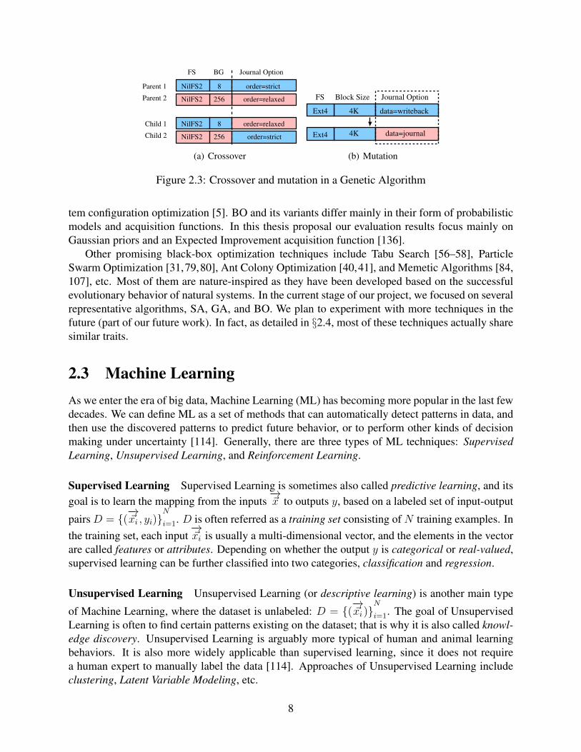
Genetic Algorithms (GA) were proposed in 1975 [70] and inspired by the process of nat-ural selection. GA maintains a population of chromosomes (configurations) and applies severalgenetic operators to them. Crossover takes two parent chromosomes and generates new ones.As Figure 2.3(a) illustrates, two parent Nilfs2 configurations are cut at the same crossover point,and then the subparts after the crossover point are exchanged between them to generate two newchild configurations. Better chromosomes will have a higher probability to “survive” in futureselection phases. Mutation randomly picks a chromosome and mutates one or more parametervalues, which produces a completely different chromosome. Figure 2.3(b) illustrates such mu-tation, where the journal option is randomly mutated from writeback to journal. GA and itsvariants have been widely applied to various areas including the Traveling Salesman Problem(TSP) [59,62,86,113,122,140], VLSI Design [16,33,99,105], High-Performance Computing [11],and system design [30, 36, 101].

Bayesian Optimization (BO) [19,136] is a popular framework to solve optimization problems.It models the objective function as a stochastic process, with the argument corresponding to onestorage configuration. In the beginning, a set of prior points (configurations) are given to the algo-rithm to get a fair estimate of the entire parameter space. BO works by computing the confidenceinterval of the objective function according to previous evaluation results. Here the confidenceinterval is the range of values that the evaluation result is most likely to fall into (e.g., with 95%probability). The next configuration is selected based on a pre-defined acquisition function. Bothconfidence intervals and the acquisition function are updated with each new evaluation. BO hasbeen successfully applied in various areas, including hyper-parameter optimization [34] and sys-

7

Parent 1

Parent 2

Child 1

Child 2

Journal OptionBG FS

NilFS2

NilFS2

8

256

order=strict

order=relaxed

order=relaxed8NilFS2

order=strict256

NilFS2

(a) Crossover

FS Journal Option

data=journal4KExt4

Block Size

Ext4 4K data=writeback

(b) Mutation

Figure 2.3: Crossover and mutation in a Genetic Algorithm

tem configuration optimization [5]. BO and its variants differ mainly in their form of probabilisticmodels and acquisition functions. In this thesis proposal our evaluation results focus mainly onGaussian priors and an Expected Improvement acquisition function [136].

Other promising black-box optimization techniques include Tabu Search [56–58], ParticleSwarm Optimization [31,79,80], Ant Colony Optimization [40,41], and Memetic Algorithms [84,107], etc. Most of them are nature-inspired as they have been developed based on the successfulevolutionary behavior of natural systems. In the current stage of our project, we focused on severalrepresentative algorithms, SA, GA, and BO. We plan to experiment with more techniques in thefuture (part of our future work). In fact, as detailed in §2.4, most of these techniques actually sharesimilar traits.

2.3 Machine LearningAs we enter the era of big data, Machine Learning (ML) has becoming more popular in the last fewdecades. We can define ML as a set of methods that can automatically detect patterns in data, andthen use the discovered patterns to predict future behavior, or to perform other kinds of decisionmaking under uncertainty [114]. Generally, there are three types of ML techniques: SupervisedLearning, Unsupervised Learning, and Reinforcement Learning.

Supervised Learning Supervised Learning is sometimes also called predictive learning, and itsgoal is to learn the mapping from the inputs

−→~x to outputs y, based on a labeled set of input-output

pairs D = {(−→~xi , yi)}

N

i=1. D is often referred as a training set consisting of N training examples. Inthe training set, each input

−→~xi is usually a multi-dimensional vector, and the elements in the vector

are called features or attributes. Depending on whether the output y is categorical or real-valued,supervised learning can be further classified into two categories, classification and regression.

Unsupervised Learning Unsupervised Learning (or descriptive learning) is another main type

of Machine Learning, where the dataset is unlabeled: D = {(−→~xi )}

N

i=1. The goal of UnsupervisedLearning is often to find certain patterns existing on the dataset; that is why it is also called knowl-edge discovery. Unsupervised Learning is arguably more typical of human and animal learningbehaviors. It is also more widely applicable than supervised learning, since it does not requirea human expert to manually label the data [114]. Approaches of Unsupervised Learning includeclustering, Latent Variable Modeling, etc.

8

Reinforcement Learning Reinforcement Learning (RL) [143] is an area of machine learning in-spired by behaviorist psychology. RL explores how software agents take actions in an environmentto maximize the defined cumulative rewards. Most RL algorithms can be formulated as a modelconsisting of: (1) A set of environment states; (2) A set of agent actions; and (3) A set of scalarrewards. In case of storage systems, states correspond to configurations, actions mean changing toa different configuration, and rewards are differences in evaluation results. The agent records itsprevious experience (history), and makes it available through a value function, which can be usedto predict the expected reward of state-action pairs. The policy determines how the agent takesaction. A simple example is ε-policy. For each action the agent may can take a random action withprobability ε; otherwise it will exploit the current value function and take the best action to max-imize the rewards. The value function’s history can be stored in a tabular form, but this does notscale well to many dimensions. Function approximation is one way for generalization when thestate and/or action spaces are large or continuous. However, most approximation methods are stillknown to be unstable or even divergent. With recent advances in Deep Learning [61], deep con-volutional neural networks, termed Deep Q-Networks (DQN), were proposed to parameterize thevalue function, and have been successfully applied in solving various problems [110, 111]. Manyvariants of DQN have been proposed [93]; in this proposal we applied its original version [111].Another interesting fact here is that many RL algorithms, including DQN, also maintains a trade-off between exploitation, exploration, and history. In the early stages of execution, when the agentknows little about the environment, it will explore the space and try unknown actions. When itinteracts enough with the environment, it will tend to choose the actions that it knows will receivethe higher rewards.

2.4 Unified Framework

Algorithm Origin Exploration Exploitation History

SimulatedAnnealing (SA)

Annealingtechnology in

metallurgy

Allowing movingto worse neighbor

statesNeighbor function N/A

GeneticAlgorithms (GA) Natural evolution Mutation

Crossover andselection

Currentpopulation

DeepQ-Networks

(DQN)

Behavioristpsychology and

neuroscience

Taking randomactions

Taking actionsbased on

action-rewardfunction

Deepconvolutional

neural network

BayesianOptimization

(BO)

Statistics andexperimental

design

Selecting sampleswith highvariances

Selecting sampleswith high mean

values

Acquisitionfunction &

probabilisticmodel

Table 2.1: Comparison and summaries of optimization techniques

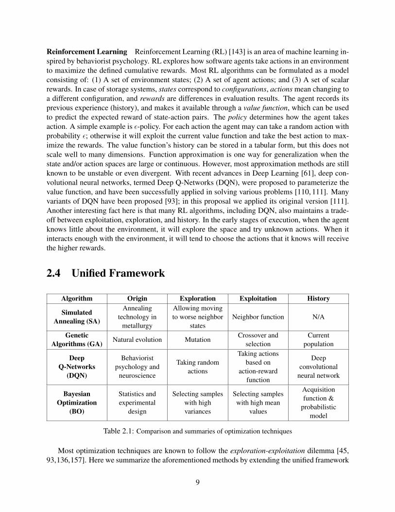
Most optimization techniques are known to follow the exploration-exploitation dilemma [45,93,136,157]. Here we summarize the aforementioned methods by extending the unified framework

9

with a third factor, the history. Our unified view thus defines three factors or dimensions:

• Exploration defines how the technique searches unvisited areas. This often includes a com-bination of pure random and also guided search.

• Exploitation defines how the technique leverages current neighborhood or history to findnext sample.

• History defines how much data from previous evaluations is kept. History information canbe used to help guide both future exploration and exploitation (e.g., avoiding less promisingregions, or selecting regions that have never been explored before).

Table 2.1 summarizes how the aforementioned techniques work by maintaining the balance amongthese three key factors. For example, GA keeps the evaluation results from the last generation,which corresponds to the concept of history in our unified framework. GA then exploits the storedinformation, applying selection and crossover to search nearby areas and pick the next generation.Occasionally, it also randomly mutates some chosen parameters, which is the idea of exploration.The trade-off among exploration, exploitation, and history largely determines the effectiveness andefficiency of these optimization techniques.

10

Chapter 3

Related Work

This chapter describes related previous work and compare them with our project.

3.1 Auto-tuning in Computer SystemsIn recent years, several attempts were made to automate the tuning of storage systems. Gaonkar etal. [53] apply GAs to design dependable data storage systems for multi-application environments,with the goal of minimizing the overall cost of the system while meeting business requirements.Strunk et al. [141] proposed to use utility functions combining different system metrics and ap-plied GA to automate storage system provisioning. Babak et al. [12] utilized GA to optimize I/Operformance of HDF5 applications. Kimberly et al. [78] formulate the data recovery schedulingproblem as an optimization problem. They aim at finding the schedule that minimizes the financialpenalties due to downtime, data loss, and vulnerability to subsequent failures. GAs are applied andcompared with several other heuristics. Xue et al. [166, 167] propose an autonomic technique thatlearns the intensity patterns of user workload in tiered storage systems over long time-scales usinga probabilistic model. They use the model to predict the coming workload patterns and proactivelystop/start bulky internal system work. MINERVA [6], is a suite of tools for automating stor-age system design, which uses declarative specifications of application requirements and devicecapabilities; constraint-based formulations of the various sub-problems; and simple bin-packingheuristics to explore the search space of possible solutions. More recently, Deep Q-Networks hasbeen successfully applied in optimizing performance for Lustre [168].

Auto-tuning is also a hot topic in other computer systems: Bayesian Optimization was appliedto find near-optimal configurations for databases [155] and Cloud VMs [5]. Other applied tech-niques include Evolutionary Strategies [126], Simulated Annealing [51, 73], Tabu Search [127],and more.

However, previous work all focused on a single algorithm or technique. One contribution ofour work is to provide the first comparative study of multiple, applicable optimization methodsand compare them for their efficacy in auto-tuning storage systems from various aspects. We alsoprovide some insights into the working mechanism of auto-tuning. More importantly, we proposeto design a more intelligent and practical framework for auto-tuning storage systems in real-time.

11

3.2 Hyper-parameter tuningEsteban et al. [119] applied Evolutionary Algorithms to hyper-parameter optimization for neuralnetworks, and achieved state-of-art results on certain data-sets. Bergstra and Bengio [15] foundthat randomly chosen trials are more efficient for hyper-parameter optimization than trials on agrid, and explained the cause as the objective function having a low effective dimensionality. Inaddition, Reinforcement Learning [13] and Bayesian Optimization [44] were also applied to hyper-parameter optimization. Another direction of research focuses on eliminating all hyper-parametersand tries to propose non-parametric versions of optimization methods. Examples of this includeGA [66, 100] and BO [136]

In this work, we will investigate the impacts of hyper-parameters on various optimization tech-niques, when applied to auto-tune storage systems.

3.3 Workload ModelingA few efforts have been made on modeling or characterizing storage workloads. Bumjoon etal. [133] tried to model storage workloads on HDDs from a data-mining point of view. They usea unique clustering method for feature selection that reduces computational time on a list of 20features available through blktrace and use a hierarchy of clustering and classification to label aworkload based on access patterns. Busch et al. [21] proposed to design an automated approach forextracting workload models in virtualized environments. Features used include average file size,file set size, average request size, etc. Li et al. [90] attempted to better define sequential I/O. Theyfocused on LBA and I/O size, and concluded that “consecutive bytes accessed” should be taken intoconsideration. Shen et al. [138] characterized workloads with the goal of improving performancedebugging by separating their model into OS caching, prefetching, OS I/O Scheduling, and storagedevices. Wang et al. [158] used CART models to predict per-request response time based onworkload characteristics, and provides detailed explanations about how CART models work andwhy they are suitable for this problem. Riska et al. [123] tried to characterize workloads based ontheir environment: enterprise, desktop, or consumer electronics.

We feel that most previous work were either vague on what features to pick for characterizingworkload, or they limited the model built to one or few use cases. In this work, we target atfinding the minimum set, or a small-enough set of features (out of many), which is general and cancharacterize most storage workload. The feature engineering work will utilize cutting-edge MLand data mining techniques, but we will explain out observations from storage perspective as well.

12

Chapter 4

Experimental Settings

In this chapter we detail the experimental environments, parameter spaces, and our implementa-tions of several optimization algorithms.

4.1 HardwareWe performed experiments on two sets of machines with different hardware categorized as low-end (S1) and mid-range (S2). We list the details of these two sets of machines in Table 4.1. We alsouse Watts Up Pro ES power meters to measure the energy consumption. During our experimentson characterizing storage performance variation (Chapter 6), to maintain realistically high ratio ofthe dataset size to the RAM size and ensure that our experiments produce enough I/O, we limitedthe RAM size on all machines to 4GB. We denote this hardware setting as S3. We have one typeof storage device on S1 and four others on S2 and S3, which will be denoted as HDD1, HDD2,HDD3, HDD4, and SSD for short in this proposal.

4.2 WorkloadWe used Filebench [50,149] to generate various workloads in our experiments. In each experiment,if not stated otherwise, we formatted and mounted the storage devices with a file system and thenran Filebench. We mainly experimented with the four pre-configured Filebench macro-workloadsthat exhibit the following significantly different I/O properties:

• Mailserver emulates the I/O workload of a multi-threaded email server. It generates se-quences of I/O operations that mimic the behavior of reading emails (open, read the wholefile, and close), composing emails (open/create, append, close, and fsync) and deletingemails. It uses a flat directory structure with all the files in a single directory, and thusexercises the ability of file systems to support large directories and fast lookups.

• Fileserver emulates the I/O workload of a server that hosts users’ home directories. Here,each thread represents a user, which performs create, delete, append, read, write, and statoperations on a unique set of files. It exercises both the metadata and data paths of thetargeted file system.

13

Setting S1 S2 S3

Model Dell PowerEdgeSC1425

Dell PowerEdge R710 Dell PowerEdge R710

CPU Intel Xeon single-core2.8GHz CPU × 2

Intel Xeon quad-core2.4GHz CPU × 2

Intel Xeon quad-core2.4GHz CPU × 2

Memory 2GB 24GB4GB (set by mem= in

/etc/default/grub)

StorageHDD1 (73GB SeagateST373207LW SCSI

drive) × 2

HDD2 (146GB SeagateST9146853SS SAS

HDD), HDD3 (500GBSeagate ST9500430SS

SAS HDD), HDD4(200GB Intel

SSDSC2BA200G3SATA HDD), SSD

(250GB FujitsuMHZ2250BKG2 SATA

HDD)

HDD2 (146GB SeagateST9146853SS SAS

HDD), HDD3 (500GBSeagate ST9500430SS

SAS HDD), HDD4(200GB Intel

SSDSC2BA200G3SATA HDD), SSD

(250GB FujitsuMHZ2250BKG2 SATA

HDD)Partition 100GB 100GB Full size

OS Ubuntu 14.04 withkernel 3.13

Ubuntu 14.04 withkernel 3.13

Ubuntu 14.04 withkernel 4.4

Table 4.1: Details of experiment machines.

• Webserver emulates the I/O workload of a typical static Web server with a high percentageof reads. Files (Web pages) are read sequentially by multiple threads (users); each threadappends to a common log file (Web log). This workload exercises fast lookups, sequentialreads of small files and concurrent data and metadata management.

• Dbserver mimics the behaviors of Online Transaction Processing (OLTP) databases. Itmainly consists of random asynchronous writes, random asynchronous reads and moderatesynchronous writes to the log file. It exercises the ability of large file management, extensiveconcurrency, and random read/write operations.

Workload Avg. Avg. Dir # Running Num. of R/W FilebenchFile Size Width Files Time (s) Threads Ratio Version

fileserver-def 128KB 20 10,000 100 50 1:2 1.4.9mailserver-def 16KB 1,000 1,000 100 16 1:1 1.4.9webserver-def 16KB 20 1,000 100 100 10:1 1.4.9dbserver-def 10MB 1,024 10 100 10 + 1 10:1 1.4.9

fileserver-heavy 128KB 20 80,000 800 50 1:2 1.5.0mailserver-heavy 16KB 1,000,000 640,000 2,000 16 1:1 1.5.0webserver-heavy 16KB 20 640,000 800 100 10:1 1.5.0

Table 4.2: Filebench workload characteristics.

14

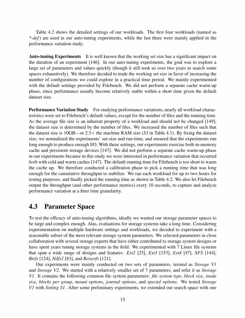
Table 4.2 shows the detailed settings of our workloads. The first four workloads (named as*-def ) are used in our auto-tuning experiments, while the last three were mainly applied in theperformance variation study.

Auto-tuning Experiments It is well known that the working set size has a significant impact onthe duration of an experiment [146]. In our auto-tuning experiments, the goal was to explore alarge set of parameters and values quickly (though it still took us over two years to search somespaces exhaustively). We therefore decided to trade the working set size in favor of increasing thenumber of configurations we could explore in a practical time period. We mainly experimentedwith the default settings provided by Filebench. We did not perform a separate cache warm-upphase, since performance usually become relatively stable within a short time given the defaultdataset size.

Performance Variation Study For studying performance variations, nearly all workload charac-teristics were set to Filebench’s default values, except for the number of files and the running time.As the average file size is an inherent property of a workload and should not be changed [149],the dataset size is determined by the number of files. We increased the number of files such thatthe dataset size is 10GB—or 2.5× the machine RAM size (S3 in Table 4.1). By fixing the datasetsize, we normalized the experiments’ set-size and run-time, and ensured that the experiments runlong enough to produce enough I/O. With these settings, our experiments exercise both in-memorycache and persistent storage devices [147]. We did not perform a separate cache warm-up phasein our experiments because in this study we were interested in performance variation that occurredboth with cold and warm caches [147]. The default running time for Filebench is too short to warmthe cache up. We therefore conducted a calibration phase to pick a running time that was longenough for the cumulative throughput to stabilize. We ran each workload for up to two hours fortesting purposes, and finally picked the running time as shown in Table 4.2. We also let Filebenchoutput the throughput (and other performance metrics) every 10 seconds, to capture and analyzeperformance variation at a finer time granularity.

4.3 Parameter SpaceTo test the efficacy of auto-tuning algorithms, ideally we wanted our storage parameter spaces tobe large and complex enough. Alas, evaluations for storage systems take a long time. Consideringexperimentation on multiple hardware settings and workloads, we decided to experiment with areasonable subset of the most relevant storage system parameters. We selected parameters in closecollaboration with several storage experts that have either contributed to storage system designs orhave spent years tuning storage systems in the field. We experimented with 7 Linux file systemsthat span a wide range of designs and features: Ext2 [25], Ext3 [153], Ext4 [47], XFS [144],Btrfs [124], Nilfs2 [83], and Reiserfs [121].

Our experiments were mainly conducted on two sets of parameters, termed as Storage V1and Storage V2. We started with a relatively smaller set of 7 parameters, and refer it as StorageV1. It contains the following common file system parameters: file system type, block size, inodesize, blocks per group, mount options, journal options, and special options. We tested StorageV1 with Setting S1. After some preliminary experiments, we extended our search space with one

15

Param. Abbr. ValuesFile System FS Ext2, Ext3, Ext4, XFS, Btrfs, Nilfs2, Reiserfs

Block Size, Leaf Size BS 1K, 2K, 4KInode Size, Sector Size IS n/a, 128, 256, 512, 1024, 2048, 4096, 8192

Block Group, Alloc. Group BG n/a, 2, 4, 8, 16, 32, 64, 128, 256

Journal Option JOn/a, order=strict, order=relaxed, data=journal, data=ordered,

data=writebackAtime Option AO relatime, noatimeSpecial Option SO n/a, compress, nodatacow, nodatasum, notailI/O Scheduler I/O noop, cfq, deadline

Table 4.3: Details of Parameter Spaces

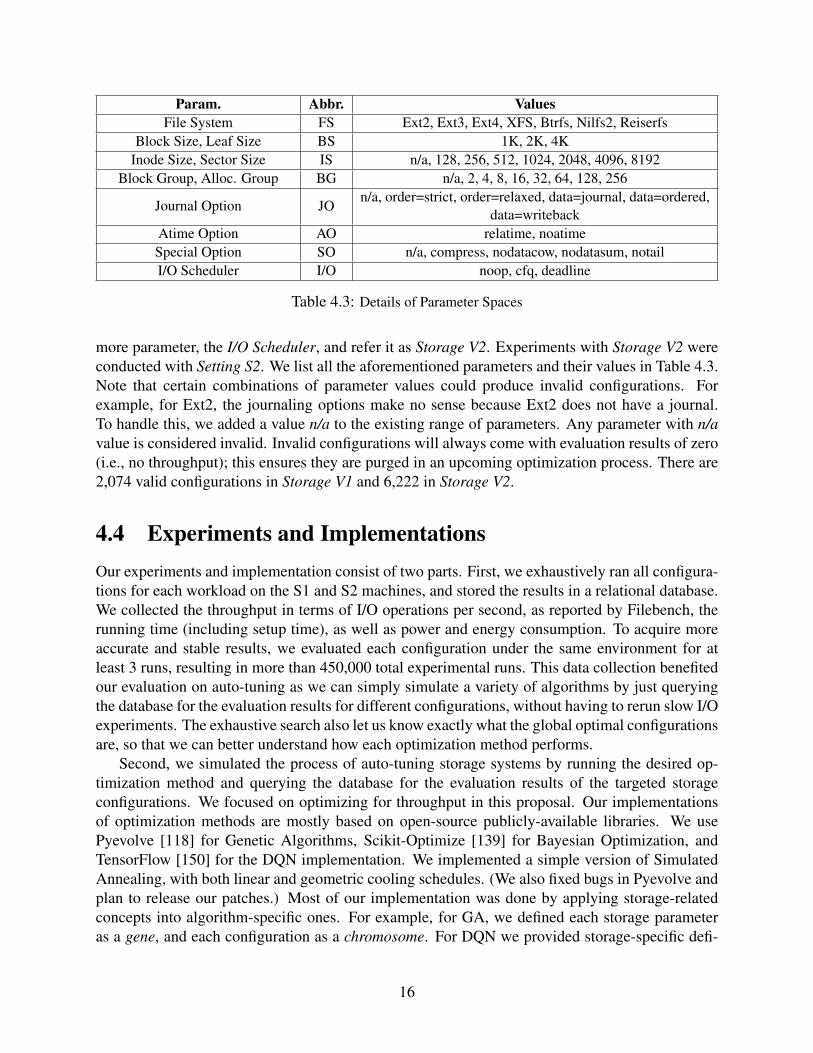
more parameter, the I/O Scheduler, and refer it as Storage V2. Experiments with Storage V2 wereconducted with Setting S2. We list all the aforementioned parameters and their values in Table 4.3.Note that certain combinations of parameter values could produce invalid configurations. Forexample, for Ext2, the journaling options make no sense because Ext2 does not have a journal.To handle this, we added a value n/a to the existing range of parameters. Any parameter with n/avalue is considered invalid. Invalid configurations will always come with evaluation results of zero(i.e., no throughput); this ensures they are purged in an upcoming optimization process. There are2,074 valid configurations in Storage V1 and 6,222 in Storage V2.

4.4 Experiments and ImplementationsOur experiments and implementation consist of two parts. First, we exhaustively ran all configura-tions for each workload on the S1 and S2 machines, and stored the results in a relational database.We collected the throughput in terms of I/O operations per second, as reported by Filebench, therunning time (including setup time), as well as power and energy consumption. To acquire moreaccurate and stable results, we evaluated each configuration under the same environment for atleast 3 runs, resulting in more than 450,000 total experimental runs. This data collection benefitedour evaluation on auto-tuning as we can simply simulate a variety of algorithms by just queryingthe database for the evaluation results for different configurations, without having to rerun slow I/Oexperiments. The exhaustive search also let us know exactly what the global optimal configurationsare, so that we can better understand how each optimization method performs.

Second, we simulated the process of auto-tuning storage systems by running the desired op-timization method and querying the database for the evaluation results of the targeted storageconfigurations. We focused on optimizing for throughput in this proposal. Our implementationsof optimization methods are mostly based on open-source publicly-available libraries. We usePyevolve [118] for Genetic Algorithms, Scikit-Optimize [139] for Bayesian Optimization, andTensorFlow [150] for the DQN implementation. We implemented a simple version of SimulatedAnnealing, with both linear and geometric cooling schedules. (We also fixed bugs in Pyevolve andplan to release our patches.) Most of our implementation was done by applying storage-relatedconcepts into algorithm-specific ones. For example, for GA, we defined each storage parameteras a gene, and each configuration as a chromosome. For DQN we provided storage-specific defi-

16

nitions for states, actions, and rewards. The complete implementation uses around 8,000 lines ofcode, consisting of Python and Shell scripts.

17

Chapter 5

Towards Better Understanding of Black-boxAuto-Tuning: A Comparative Analysis forStorage Systems

In this chapter we apply several popular techniques to the collected dataset to find optimal config-urations under various hardware and workload settings: Simulated Annealing (SA), Genetic Algo-rithms (GA), Bayesian Optimization (BO), and Deep Q-Networks (DQN). We also tried RandomSearch (RS) in our experiments, which showed surprisingly good results in previous research [15].We compared these techniques from various aspects, such as the ability to find near-optimal con-figurations, convergence time, and instantaneous system throughput during auto-tuning. We alsoshowed that hyper-parameter settings of these optimization algorithms, such as mutation rate inGA, could affect the tuning results. We compared the techniques across three behavioral dimen-sions: (1) Exploration: how much the technique searches the space randomly. (2) Exploitation:how much the technique leverages the “neighborhood” of the current candidate or previous searchhistory to find even better configurations. (3) History: how much data from previous evaluationsis kept and utilized in the overall search process. Based on our evaluation results, we show thatall techniques employ these three key concepts to varying degrees and the trade-off among themplays an important role in the effectiveness and efficiency of the algorithms.

Most black-box optimization methods lack solid theoretical understanding, partially due tothe large variety of problems that they were proposed to solve [170]. Based on our experimentalresults and domain expertise, we provide explanations of efficacy of such black-box optimizationmethods from a storage perspective. We observed that certain parameters would have a greatereffect on system performance than others, and the set of dominant parameters depends on filesystems and workloads. This allows us to provide more insights into the auto-tuning process.

Part of the results from this chapter will be published in ATC 2018.The chapter is organized as follows. Chapter 5.1 overviews the datasets that we collected for

over two years. Chapter 5.2 compares five popular optimization techniques from several aspects.Chapter 5.3 uses GA as a case study to show that hyper-parameters of these methods could alsoimpact the auto-tuning results.

18

5.1 Overview of Datasets

0

0.2

0.4

0.6

0.8

1

0% 20% 40% 60% 80% 100%

Norm

aliz

ed T

hro

ughput

Percentage of ConfigurationsS2, fileserver-def, HDD3

S2, mailserver-def, HDD3S2, mailserver-def, SSD

S1, mailserver-def, HDD1S2, dbserver-def, SSD

S2, webserver-def, SSD

Figure 5.1: Throughput CDF with different hardware and workloads, with symbols marking thedefault configurations.

As per Chapter 4, our experimental methodology is to first exhaustively run all configurationsunder different workloads and test machines. We stored the results in a database for future use.This data collection benefits future experiments as we can simulate a variety of algorithms byquerying the database for the evaluation results of different configurations.

Figure 5.1 shows the throughput CDF among all configurations for each hardware setting andworkload. Due to space limits, we show only 6 representative datasets out of 18 here. The Yaxis is normalized by the maximum throughput under each experiment setting. The symbols oneach line mark the default configurations. As seen, for most settings, throughput values varyacross a wide range. The ratios of the worst throughput to the best one are mostly between 0.2–0.4. In one extreme case, for fileserver-def on S1 machines and with HDD1 device, the worstconfiguration only produces 1% I/O operations per unit time, compared with the global optimalone. This underlines the importance of tuning storage systems: an improperly configured systemcould be remarkably under-utilized, and thus wasting a lot of resources. However, S2, webserver-def, SSD shows a much narrower range of throughput, with the worst-to-best ratio close to 0.9. Thisis attributed mainly to the fact that webserver-def consists of mostly sequential read operationsthat are processed similarly by different I/O stack configurations. Another useful observation fromFigure 5.1 is that default configurations are always sub-optimal and, under most settings, rankedlower than the top 40% configurations. For S1, fileserver-def, HDD1, the default configurationshows a normalized throughput of 0.39, which means that the optimal configuration performs 2.5times better.

We list the optimal configurations for each hardware setting and workload from our datasets inTable 5.1. As we can see, optimal configurations depend on the specific hardware as well as therunning workload. For mailserver-def with S1 machines and the HDD1, the global best is a Nilfs2configuration. However, if we fix the workload and change the hardware to S2-HDD3, the optimumbecomes an Ext4 configuration. Similarly, fixing the hardware to S2-SSD and experimenting under

19

Hardware File Block Inode BG Journal Atime Special I/O Through-Workload-Device System Size Size Count Options Options Options Scheduler put (IOPS)S1-Mail-HDD1 Nilfs2 2K n/a 256 order=relaxed relatime n/a - 3,677S2-Mail-HDD3 Ext2 4K 256 32 n/a relatime n/a noop 18,744S2-Mail-SSD Ext2 4K 256 8 n/a relatime n/a noop 18,845S2-File-SSD Btrfs 4K 4,096 n/a n/a relatime nodatacow deadline 16,587S2-DB-SSD Ext4 1K 128 2 data=ordered noatime n/a noop 41,948

S2-Web-SSD Ext4 4K 128 4 data=ordered noatime n/a noop 16,185

Table 5.1: Global optimal configurations with different settings and workloads. Workloads are abbreviated.Db: dbserver-def; File: fileserver-def; Mail: mailserver-def; Web: webserver-def.

different workloads leads to different optimal configurations. This proves our early claim thatperformance (and other metrics) are sensitive to the environment (i.e., hardware, configuration,and workloads); this actually complicates the problem as results from one environment cannot bedirectly applied in another.

It is known that the working set size has a significant impact on the duration of an experi-ment [146]. Our goal in this study was to explore a large set of parameters and values quickly(though it still took us over two years). We therefore decided to trade the working set size in favorof increasing the number of configurations we could explore in a practical time period. In ourexperimental results, this trade-off sometimes manifests itself since SSD configurations producecomparable throughputs as HDD ones (see Table 5.1). The experiments, however, do demonstratea wide range of performance numbers and, therefore, are valid for evaluating different optimiza-tion methods. We plan to include the working set size in the set of optimization parameters in thefuture.

5.2 Comparative AnalysisMany optimization techniques have been applied to various auto-tuning tasks [141, 155]. How-ever, previous efforts picked algorithms somewhat arbitrarily and evaluated only one algorithm ata time. Here we provide the first comparative study of multiple black-box optimization techniqueson auto-tuning storage systems. As discussed in §2.2, we focus our evaluations on a representativeset of optimization methods, and their common hyper-parameter settings, including 1) SimulatedAnnealing (SA), with a linear cooling schedule; 2) Genetic Algorithms (GAs) with population sizeof 8, mutation rate of 2%; 3) Deep Q-Networks (DQN) with experience replay [111] and ε = 0.2;and 4) Bayesian Optimization (BO) with Expected Improvement (EI) and Gaussian prior. 5) Ran-dom Search (RS), which merely performs random selection without replacement. We provide morediscussion on the impact of hyper-parameters in Chapter 5.3. Note that SA, DQN, and RS exper-iments start with the default Ext4 configuration. GA and BO require several initial configurations(prior points), which we set to default configurations of all seven file systems. This allows us tosimulate real-world use cases, where users often deploy their system with the default settings (andmay manually optimize starting from the defaults).

Figure 5.2 presents one simulated run of each optimization method on S2, mailserver-def,HDD3; the Y axis shows the throughput value of the best configuration found so far, and the

20

16

17

18

0 1 2 3 4 5

Bes

tT

hro

ug

hp

ut

(ko

ps/

s)

Time (hrs)

15.2

18.7

S2, mailserver-def, HDD3

GASABO

DQNRS

Figure 5.2: Highest throughput found over time, zooming in the Y ∈ [15 : 19] range. The bluenumber (15.2) on the Y axis shows the default, and the red one (18.7) shows the optimal.

X axis is the running time. All time-related metrics in this chapter are based on the actual run-ning time of evaluating each storage configuration, which is stored in our database. This includesboth setup time and benchmarking time. We are not comparing the running costs (including anynecessary training phases) for optimization methods here, which is our future work. Figure 5.2 isplotted by zooming in the range of Y ∈ [15 : 19], with the blue number (15.2) on Y axis repre-sents the default, while the red one (18.7) shows the global optimal. It shows that all five methodswere able to gradually find better configurations, but their effectiveness and efficiency differed alot. SA performed the worst, and got stuck in a configuration with throughput value of less than18K IOps. DQN was able to converge to a good configuration, but spent more time to achieve thatthan RS. GA and BO performed best out of these five tested optimization methods. They both suc-cessfully identified a near-optimal configuration within one hour. Interestingly, we observed thatpure Random Search (RS) produced better results than some other optimization methods. This isbecause not all storage parameters have significant impact on system performance, resulting in aneffective search space that is much smaller than the original one. Similar results were observed inhyper-parameter optimization for neural networks [14]. We discuss this further in §5.4.

Since exploration is one critical component of all optimization methods (see §2.4), their evalu-ation results could also exhibit some degree of randomness. To compare them more thoroughly, weran each optimization technique on the same environment (S2, HDD3) for 1,000 runs. Figure 5.3shows the results, which evaluate the techniques’ probability to find good and near-optimal config-urations. Here we define a near-optimal configuration as one with throughput higher than 99% ofthe global optimal value. The Y axis shows the percentage of total runs that found a near-optimalconfiguration within a certain time (X axis). Under mailserver-def workload, seen in the upperpart of Figure 5.3, SA had the lowest probability among 5 algorithms.

Even after 5 hours, only around 80% of its runs found one near-optimal configuration, whichsuggests that SA can sometimes get stuck in a local optima. For other optimization methods,given enough time, over 90% of their runs converged to a near-optimal configuration, with BOoutperforming GA, and GA outperforming DQN. RS shows the highest probability of findingnear-optimal configurations when approaching 5 hours. This is reasonable because given enoughtime, a random selection will eventually hit near-optimal points. However, when conducting the

21

20%

40%

60%

80%

100%

Per

cen

tag

e o

f R

un

s S2, mailserver-def, HDD3

RSSAGA

DQNBO

20%

40%

60%

80%

100%

0 1 2 3 4 5

Per

cen

tag

e o

f R

un

s

Time (hrs)

S2, fileserver-def, HDD3

Figure 5.3: Comparing optimization methods’ efficacy in finding near-optimal configurations. TheY axis shows the percentage of total runs (1,000) that found near-optimal configurations withincertain time (X axis).

22

same experiments under the fileserver-def workload, it becomes more difficult to find near-optimalconfigurations. GA and BO are still the best, though only 65% of their runs were able to find near-optimal configurations within 5 hours. SA, RS, and DQN have a probability of lower than 40% todo so, with DQN perform the worst. This is because the global optimum under fileserver-def isa Btrfs configuration (see Table 5.1). It is more difficult for optimization algorithms to pick suchconfigurations for the following reasons: 1) Few Btrfs configurations reside in the neighborhoodof the default Ext4 configurations; 2) Fewer than 2 % of all valid configurations are Btrfs ones,which make them less likely to be selected through mutation.

The above results all focused on finding near-optimal configurations. However, another impor-tant aspect to compare is the system’s performance during the auto-tuning process. This is espe-cially important if the targeted system is deployed and online. Some randomness (exploration) isnecessary when searching a complex parameter space, but ideally optimization algorithms shouldspend less time on bad configurations. To compare this, in Figure 5.4 we plotted the instantaneousthroughput (Y axis) over time (X axis) for one run with each method under S2, mailserver-def,HDD3.

BO and GA are still the best two methods in terms of instantaneous throughput.

51015

RS


51015

SA


51015

Thro

ughput

(kops/

s)

GA


51015

DQN


0 1 2 3 4 5

BO

Time (hrs)


Figure 5.4: Comparing optimization methods’ instantaneous performance (Y axis) over time (Xaxis).

During the tuning process, occasionally they will pick a worse configurations than the currentone. However, they both possess the ability to quickly discard these unpromising configurations.GA achieves this by assigning the probability of surviving to next generation based on the fitnessvalues (i.e., throughput). Configurations with low throughput values have a lower chance to bepicked as parents, and thus their genes (parameter values) have a lower chance of appearing inconfigurations of the next generation (i.e., “survival of the fittest”). The reason for stable instanta-neous throughputs with BO is that it uses an intelligent acquisition function to guide the selection

23

of the next generation, with the goal of maximizing the potential gain; this makes BO less likelyto choose a bad configuration. In contrast, SA performs poorly possibly because it lacks a historyto guide the exploitation and exploration phases, and only uses its neighborhood information (andcurrent temperature) to pick the next configuration. DQN shows similar results with RS, which islikely caused by the fact that DQN was originally designed as an agent interacting with an unknownenvironment, and thus a lot of exploration (randomness) occurs in the training phase [111, 168].

In conclusion, BO and GA perform best among the 5 tested methods, on either the ability toconverge to near-optimal configurations or in maintaining stable instantaneous performance duringthe tuning process. DQN and SA can find good configurations, although they were less efficientand less stable. Surprisingly, Random Search sometimes can produce better results than sometraditional optimization methods, given enough time. We provide more explanations on thesemethods in Chapter 5.4.

5.3 Impact of Hyper-ParametersMany optimization methods’ efficacy depend on the specific hyper-parameter settings, and choos-ing the right hyper-parameters has caused headache to researchers for a long time [14, 15]. In thissection we use GA as a case study, and show the impact of one hyper-parameter, the mutation rate,on auto-tuning results.

0%

20%

40%

60%

80%

100%

0 2 4 6 8 10

Per

cen

tag

e o

f R

un

s

Time (hrs)

1%2%4%8%

16%32%64%

Figure 5.5: Impact of mutation rates on GA.

The mutation rate controls the probability of randomly mutating one parameter to a differentvalue, and aligns with the idea of exploration, as per §2.4.

Figure 5.5 shows the results from 7 sets of GA experiments with different mutation rates (from1% to 64%) under S2, mailserver-def, HDD3. Each experiment was repeated for 1,000 runs.

It is similar to Figure 5.3, but with the goal of finding near-optimal configurations whosethroughput values are higher than 99.5% of the global optimal. This makes the optimization morechallenging, as GA already performs quite well on easier tasks (Chapter 5.2). As shown in thefigure, when increasing the mutation rate, GA has a higher probability to converge to near-optimalconfigurations within a shorter time period. This is because GA works by identifying promisingcombination of alleles (parameter values) for the subset of effective genes (parameters). We defineeffective parameters as those having a higher impact on performance than all others. A highermutation rate means a higher chances of exploration, and thus finding combinations of effective

24

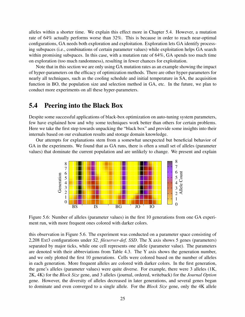
alleles within a shorter time. We explain this effect more in Chapter 5.4. However, a mutationrate of 64% actually performs worse than 32%. This is because in order to reach near-optimalconfigurations, GA needs both exploration and exploitation. Exploration lets GA identify process-ing subspaces (i.e., combinations of certain parameter values) while exploitation helps GA searchwithin promising subspaces. In this case, with a mutation rate of 64%, GA spends too much timeon exploration (too much randomness), resulting in fewer chances for exploitation.

Note that in this section we are only using GA mutation rates as an example showing the impactof hyper-parameters on the efficacy of optimization methods. There are other hyper-parameters fornearly all techniques, such as the cooling schedule and initial temperature in SA, the acquisitionfunction in BO, the population size and selection method in GA, etc. In the future, we plan toconduct more experiments on all these hyper-parameters.

5.4 Peering into the Black BoxDespite some successful applications of black-box optimization on auto-tuning system parameters,few have explained how and why some techniques work better than others for certain problems.Here we take the first step towards unpacking the “black box” and provide some insights into theirinternals based on our evaluation results and storage domain knowledge.

Our attempts for explanations stem from a somewhat unexpected but beneficial behavior ofGA in the experiments. We found that as GA runs, there is often a small set of alleles (parametervalues) that dominate the current population and are unlikely to change. We present and explain

Genera

tion

BS IS BG JO IO

0

1

2

3

4

5

6

7

8

0

1

2

3

4

5

6

7

8

All

ele

Count

Figure 5.6: Number of alleles (parameter values) in the first 10 generations from one GA experi-ment run, with more frequent ones colored with darker colors.

this observation in Figure 5.6. The experiment was conducted on a parameter space consisting of2,208 Ext3 configurations under S2, fileserver-def, SSD. The X axis shows 5 genes (parameters)separated by major ticks, while one cell represents one allele (parameter value). The parametersare denoted with their abbreviations from Table 4.3. The Y axis shows the generation number,and we only plotted the first 10 generations. Cells were colored based on the number of allelesin each generation. More frequent alleles are colored with darker colors. In the first generation,the gene’s alleles (parameter values) were quite diverse. For example, there were 3 alleles (1K,2K, 4K) for the Block Size gene, and 3 alleles (journal, ordered, writeback) for the Journal Optiongene. However, the diversity of alleles decreased in later generations, and several genes beganto dominate and even converged to a single allele. For the Block Size gene, only the 4K allele

25

survived and other two became extinct. Since GA was proposed by simulating the process ofnatural selection, where alleles with better fitness are more likely to survive, this suggests that GAworks by identifying the combination of good alleles (storage parameter values), and producingoffspring with these alleles. As shown in Figure 5.6, in the 10th generation, all configurations havea Block Size of 4K and Journal Option of writeback.

To confirm the above observations, in Figure 5.7 we plotted all Ext3-SSD configurations underfileserver-def workload, with one dot corresponding to one configuration. Configurations are sep-arated based on the Journal Option, shown as the X axis, and colored based on their Block Size. Toclearly see all points within each X-axis section, we ordered configurations by their unique iden-tification number in our database. The Y axis represents throughput values. This resulted in theformation of nine “clusters” on the graph, each corresponding to a fixed 〈Journal Option, BlockSize〉 pair. We can see that configurations with data=ordered tend to produce higher throughputthan those with data=journal, and data=writeback produces the best throughput. This is somewhatexpected from a storage point of view, as Ext3’s more fault tolerant journal option (data=journal)may hurt throughput by writing data as well as meta-data to the journal first.

0

5

10

15

data=journal data=ordered data=writeback

Th

rou

gh

pu

t (k

op

s/s)

bs=1Kbs=2Kbs=4K

Figure 5.7: Scatter plot for all Ext3-SSD configurations under fileserver-def workload, with onedot corresponding to one configuration.

Moreover, among journal configurations with data=writeback, those with a 4K Block Size turnout to produce the highest throughput. This aligns with our observation from Figure 5.6 that GAworks by identifying a subset of genes that have a greater impact on performance—Block Size andJournal Option—and finding the best alleles for them ([4K, data=writeback]).

Based on these observations, one interesting question to ask is whether the conclusion that asubset of parameter have greater impact on performance than other parameters, also holds for otherfile systems and workloads. To answer this question, we quantified the correlation between param-eter values and the throughput. As most of our parameters are categorical or discrete numeric,whereas the throughput is continuous, we took a common approach to quantify the correlationbetween categorical and continuous variables [26]. We illustrate with the Block Size parameter asan example. Since it can take 3 values, we convert this parameter to three binary variables x1, x2,and x3. If the Block Size is 1K, we assign x1 = 1 and x2 and x3 are set to 0. Let Y representthe throughput values. We then do a linear regression with ordinary least squares (OLS) on Y andx1, x2, x3. R2 is a common metric in statistics to measure how the data fits a regression line. In ourapproach, R2 actually quantifies the correlation between the selected parameter and throughput.We consider R2 > 0.6 as an indication that the parameter has significant impact on performance,as is common in statistics [26]. The same calculation is applied to all parameters among SSD

26

configurations under the fileserver-def and dbserver-def. Parameters with the highest R2 valuesare colored in yellow background in Table 5.2. If all R2 values are below 0.6, we simply leave theentries blank, meaning no highly correlated parameters were found. To find the second importantparameter, the same process is applied to the remaining parameters, but with the value of the mostimportant one fixed (to isolate its effect on the remaining parameters’ importance). Taking Ext4 asan example, we calculate R2 values for all other parameters among configurations with the sameJournal Option. For one parameter, 3 Journal Options lead to three R2 values; we then take themaximum one as the R2 value for this parameter. We color the parameter with the highest R2 inTable 5.2 with a green background.

Workload FS BS IS BG JO AO SO I/O

fileserver-def Ext2 - - - - - - 0.68Ext3 0.84 - - 0.90 - - -Ext4 0.92 - - 0.99 - - -XFS 0.94 - 0.82 - - - -Btrfs - - - - - - -Nilfs2 0.99 - - - - - 0.94

Reiserfs - - - 0.74 - - 0.99

dbserver-def Ext2 - - - - - - -Ext3 0.72 - - 0.96 - - -Ext4 - - - 0.96 0.68 - -XFS - - - - - - -Btrfs - - - - - - -Nilfs2 0.62 - - - - - 0.80

Reiserfs - - - 0.99 - - -

Table 5.2: Importance of parameters (measured by R2) among SSD configurations, with the mostimportant one colored in yellow and second in green.

We can see that the correlated parameters are quite varied, and depend a lot on file systems. Forexample, under fileserver-def, the two most important parameters for Ext3 (in descending order)are Journal Option and Block Size; this aligns with our observation in Figure 5.6 and 5.7. However,for Reiserfs, the top 2 changes to I/O Scheduler and Journal Option. Interestingly, all parametersfor Btrfs come with low R2 values, which indicates that no parameter has significant impact onsystem performance under fileserver-def with Btrfs. Correlation of parameters can also depend onthe workloads. For instance, the two dominant parameters for XFS under fileserver-def are BlockSize and Allocation Group. When the workload changes to mailserver-def, all parameters for XFSseem to have minor impact on performance. Note that here we are isolating the impact of eachparameter, thus assuming that their effect on throughput is independent; in future work we plan toinvestigate whether parameters have inter-dependencies.

The fact that parameters have varied impact on performance can also help explain the auto-tuning results in Chapter 5.2. Although our parameter space comes with 8 parameters, only asubset of them are correlated with performance. The number of dominant parameters is termed aseffective dimension, and has also been observed in hyper-parameter optimization problems [14].In our experiments (Chapter 5.2), Random Search (RS) is actually searching in a smaller effec-tive space than the original one, and thus can find good configurations within a short time. GA’s

27

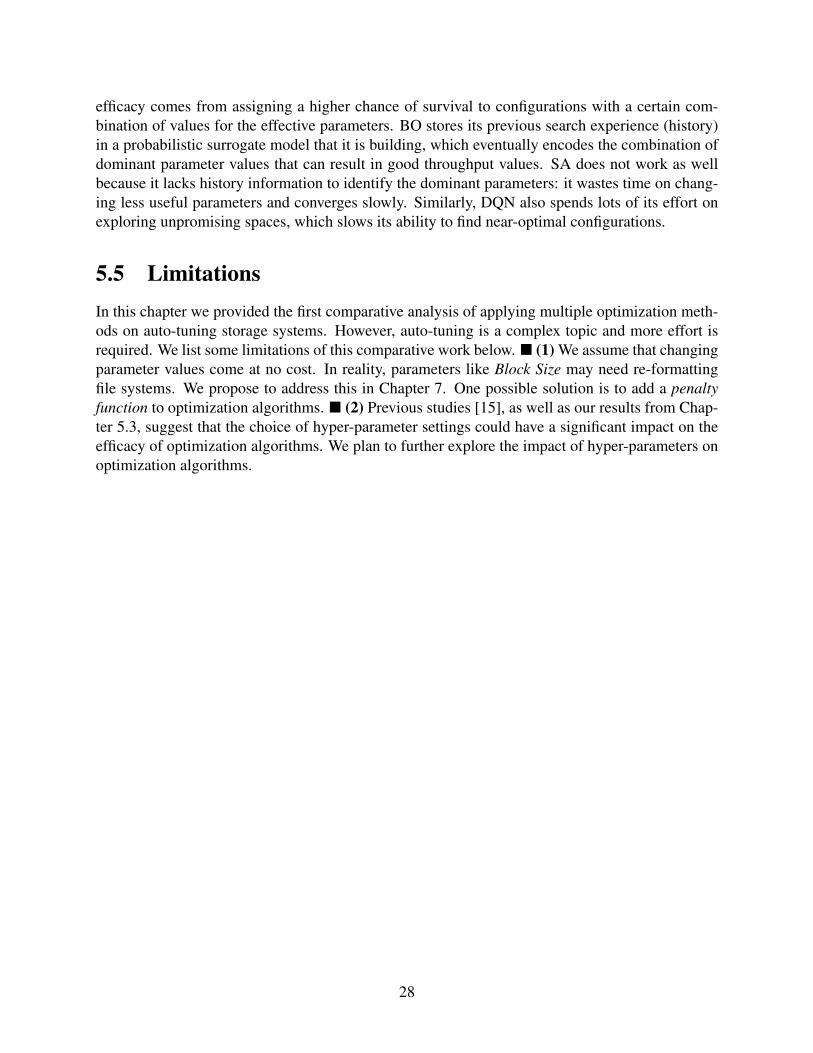
efficacy comes from assigning a higher chance of survival to configurations with a certain com-bination of values for the effective parameters. BO stores its previous search experience (history)in a probabilistic surrogate model that it is building, which eventually encodes the combination ofdominant parameter values that can result in good throughput values. SA does not work as wellbecause it lacks history information to identify the dominant parameters: it wastes time on chang-ing less useful parameters and converges slowly. Similarly, DQN also spends lots of its effort onexploring unpromising spaces, which slows its ability to find near-optimal configurations.

5.5 LimitationsIn this chapter we provided the first comparative analysis of applying multiple optimization meth-ods on auto-tuning storage systems. However, auto-tuning is a complex topic and more effort isrequired. We list some limitations of this comparative work below. � (1) We assume that changingparameter values come at no cost. In reality, parameters like Block Size may need re-formattingfile systems. We propose to address this in Chapter 7. One possible solution is to add a penaltyfunction to optimization algorithms. � (2) Previous studies [15], as well as our results from Chap-ter 5.3, suggest that the choice of hyper-parameter settings could have a significant impact on theefficacy of optimization algorithms. We plan to further explore the impact of hyper-parameters onoptimization algorithms.

28

Chapter 6

On the Performance Variation in ModernStorage Systems

6.1 MotivationsPredictable performance is critical in many modern computer environments. For instance, toachieve good user experience, which notably impacts the revenues, interactive Web services re-quire stable response time [37, 72, 91]. In cloud environments users pay for computational re-sources. Therefore, achieving predictable system performance, or at least establishing the limitsof performance variation, is of utmost importance for the clients’ satisfaction [142, 165]. In abroader sense, humans generally expect repetitive actions to yield the same results and take thesame amount of time to complete; conversely, the lack of performance stability, is fairly unsatis-factory to humans.

Performance variation is a complex issue and can arise from nearly every layer in a computersystem. At the hardware level, CPU, main memory, buses, and secondary storage can all contributeto overall performance variation [37, 91]. At the OS and middleware level, when background dae-mons and maintenance activities are scheduled, they impact the performance of deployed appli-cations. More performance disruptions come into play when considering distributed systems, asapplications on different machines have to compete for heavily shared resources, such as networkswitches [37].

In this chapter we focus on characterizing and analyzing performance variations arising frombenchmarking a typical modern storage system that consists of a file system, a block layer, andstorage hardware. Storage have been proven to be a critical contributor to performance varia-tion [67, 128, 146]. Furthermore, among all system components, the storage system is the corner-stone of data-intensive applications, which become increasingly more important in the big dataera [29,75]. Although our main focus here is reporting and analyzing the variations in benchmark-ing processes, we believe that our observations pave the way for understanding stability issues inproduction systems.

Historically, many experienced researchers noticed how workloads, software, hardware, andthe environment—even if reportedly “identical”—exhibit different degrees of performance varia-tions in repeated, controlled experiments [28, 37, 46, 91, 98]. We first encountered such variationsin exhaustive search experiments (see Chapter 4) with Ext4: multiple runs of the same workload in

29

a carefully controlled environment produced widely different performance results. Over a periodof two years of collecting performance data, we later found that such high performance varia-tions were not confined to Ext4. Over 18% of 6,222 different storage configurations on 4 differentstorage devices that we tried exhibited a standard deviation of performance larger than 5% of themean, and a range value (maximum minus minimum performance, divided by the average) exceed-ing 9%. In a few extreme cases, standard deviation exceeded 40% even with numerous repeatedexperiments. The observation that some configurations are more stable than others motivated usto conduct a more detailed study of storage system performance variation and seek its root causes,as performance stability is critical for storage systems and important in achieving the success ofauto-tuning.

To the best of our knowledge there are no systematic studies of performance variation in stor-age systems. Thus, our first goal was to characterize performance variation in different storageconfigurations. However, measuring this for even a single storage configuration is time consum-ing; and measuring all possible configurations is time-prohibitive. Even with our Storage V2 (seeChapter 4.3), it could take more than 2 years of evaluation time. Therefore, in this study we com-bined two approaches to reduce the configuration space and therefore the amount of time to runthe experiments: (1) we used domain expertise to select the most relevant parameters, and (2) weapplied a Latin Hypercube Sampling (LHS) to the configuration space. Even for the reduced space,it took us over 33 clock days to complete these experiments alone.

We focused on three local file systems (Ext4, XFS, and Btrfs) which are used in many modernlocal and distributed environments. Using our expertise, we picked several widely used parametersfor these file systems (e.g., block size, inode size, journal options). We also varied the Linux I/Oscheduler and storage devices, as they can have significant impact on performance. We bench-marked over 100 configurations using different workloads and repeated each experiment 10 timesto balance the accuracy of variation measurement with the total time taken to complete these ex-periments. We then characterized performance variation from several angles: throughput, latency,temporally, spatially, and more. We found that performance variation depends heavily on the spe-cific configuration of the system. We then further dove into the details, analyzed and explainedcertain performance variations. For example: we found that unpredictable layouts in Ext4 couldcause over 16–19% of performance variation in some cases. We discovered that the magnitudeof variation also depends on the observation window size: in one workload, 40% of XFS config-urations exhibited higher than 20% variation with a window size of 60s, but almost all of themstabilized when the window size grew to 400s. Finally, we analyzed latency variations from vari-ous aspects, and proposed a novel approach for quantifying the impacts of each operation type onoverall performance variation.

We summarize key contributions of our performance variation study as follows: � (1) To thebest of our knowledge, we are the first to provide a detailed characterization of performance vari-ation occurring in benchmarking a typical modern storage system. We believe our study pavesthe way towards the better understanding of complex storage system performance variations, inboth experimental and production settings. � (2) We conducted a comprehensive study of stor-age system performance variation. Our analysis includes throughput and latency, and both spatialand temporal variations. � (3) We offer insights into the root causes of some performance varia-tions, which could help anyone who seeks stable results from benchmarking storage systems, andencourage more follow-up work in understanding variations in production systems.

This study has been published in FAST 2017 [24]. The rest of the chapter is organized as

30

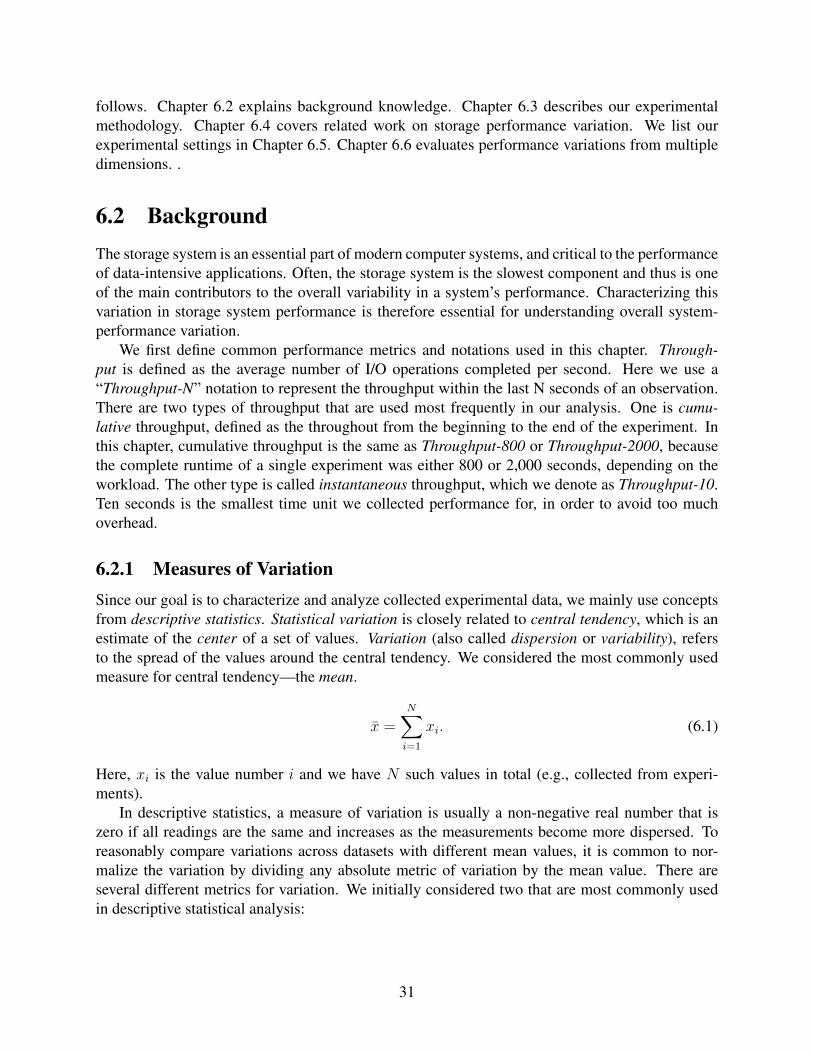
follows. Chapter 6.2 explains background knowledge. Chapter 6.3 describes our experimentalmethodology. Chapter 6.4 covers related work on storage performance variation. We list ourexperimental settings in Chapter 6.5. Chapter 6.6 evaluates performance variations from multipledimensions. .

6.2 BackgroundThe storage system is an essential part of modern computer systems, and critical to the performanceof data-intensive applications. Often, the storage system is the slowest component and thus is oneof the main contributors to the overall variability in a system’s performance. Characterizing thisvariation in storage system performance is therefore essential for understanding overall system-performance variation.

We first define common performance metrics and notations used in this chapter. Through-put is defined as the average number of I/O operations completed per second. Here we use a“Throughput-N” notation to represent the throughput within the last N seconds of an observation.There are two types of throughput that are used most frequently in our analysis. One is cumu-lative throughput, defined as the throughout from the beginning to the end of the experiment. Inthis chapter, cumulative throughput is the same as Throughput-800 or Throughput-2000, becausethe complete runtime of a single experiment was either 800 or 2,000 seconds, depending on theworkload. The other type is called instantaneous throughput, which we denote as Throughput-10.Ten seconds is the smallest time unit we collected performance for, in order to avoid too muchoverhead.

6.2.1 Measures of VariationSince our goal is to characterize and analyze collected experimental data, we mainly use conceptsfrom descriptive statistics. Statistical variation is closely related to central tendency, which is anestimate of the center of a set of values. Variation (also called dispersion or variability), refersto the spread of the values around the central tendency. We considered the most commonly usedmeasure for central tendency—the mean.

x =N∑i=1

xi. (6.1)

Here, xi is the value number i and we have N such values in total (e.g., collected from experi-ments).

In descriptive statistics, a measure of variation is usually a non-negative real number that iszero if all readings are the same and increases as the measurements become more dispersed. Toreasonably compare variations across datasets with different mean values, it is common to nor-malize the variation by dividing any absolute metric of variation by the mean value. There areseveral different metrics for variation. We initially considered two that are most commonly usedin descriptive statistical analysis:

31

• Relative Standard Deviation (RSD): the RSD, (or Coefficient of Variation (CV)) is

RSD =

√1

N−1

∑Ni=1(xi − x)2

x(6.2)

• Relative Range: this is defined as the difference between the smallest and largest values:

RelativeRange =max(X)−min(X)

x(6.3)

Because a range uses maximum and minimum values in its calculation, it is more sensitive to out-liers. We did not want to exclude or otherwise diminish the significance of performance outliers.We found that even a few long-running I/O operations can substantially worsen actual user expe-rience due to outliers (which are re-producible). Such outliers have real-world impact, especiallyas more services are offloaded to the cloud, and customers demand QoS guarantees through SLAs.That is one reason why researchers recently have begun to focus on tail latencies [37, 65, 67]. Inconsidering the two metrics above, we felt that the RSD hides some of the magnitudes of thesevariations—because using square root tends to “compress” the outliers’ values. We therefore de-cided to use the Relative Range as our main metric of variation in the rest of this chapter.

6.3 MethodologyAlthough we encountered storage system performance variations in past projects, we were espe-cially struck by this issue in our recent experiments on automated recognition of optimal storageconfigurations. We found that multiple runs of the same workload in a carefully controlled en-vironment could sometimes produce quite unstable results. We later observed that performancevariations and their magnitude depend heavily on the specific configuration of the storage system.Over 18% of 24,888 different storage configurations that we evaluated (repeatedly over severalworkloads) exhibited results with a relative range higher than 9% and relative standard deviationhigher than 5%.

Workloads also impact the degree of performance variation significantly. For the same con-figuration, experiments with different workloads could produce different magnitudes of variation.For example, we found one Btrfs configuration produces variation with over 40% relative rangevalue on one workload but only 6% for another. All these findings led us to study the character-istics and analyze performance variations in benchmarking various storage configurations undermultiple workloads. Due to the high complexity of storage systems, we have to apply certainmethodologies in designing and conducting our experiments.

Reducing the parameter space In this chapter we focus on evaluating local storage systems(e.g., Ext4, Linux block layer, SSD). This is a useful basis for studying more complex distributedstorage systems (e.g., Ceph [159], Lustre [109], GPFS [129], OpenStack Swift [117]). Even asmall variation in local storage system performance can result in significant performance fluctua-tions in large-scale distributed system that builds on it [37, 103, 112].

Despite its simple architecture, a local storage system can still have a large number of param-eters at every layer, resulting in a vast number of possible configurations. For instance, common

32

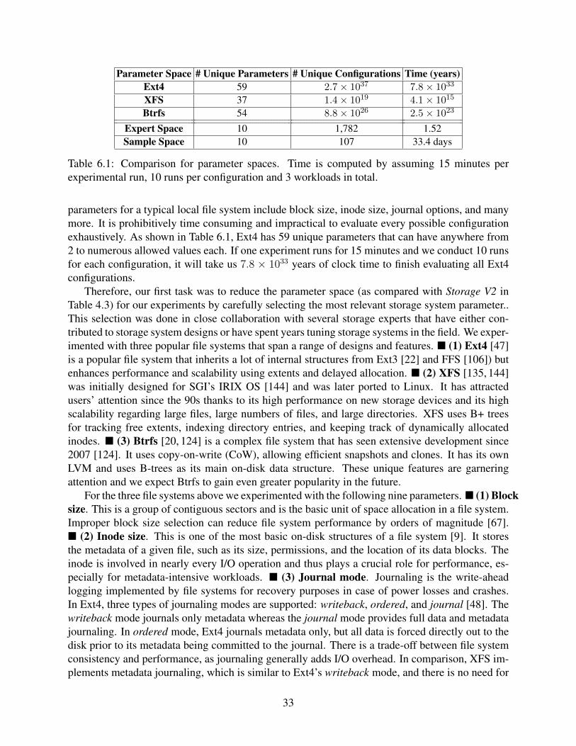
Parameter Space # Unique Parameters # Unique Configurations Time (years)Ext4 59 2.7× 1037 7.8× 1033

XFS 37 1.4× 1019 4.1× 1015

Btrfs 54 8.8× 1026 2.5× 1023

Expert Space 10 1,782 1.52Sample Space 10 107 33.4 days

Table 6.1: Comparison for parameter spaces. Time is computed by assuming 15 minutes perexperimental run, 10 runs per configuration and 3 workloads in total.

parameters for a typical local file system include block size, inode size, journal options, and manymore. It is prohibitively time consuming and impractical to evaluate every possible configurationexhaustively. As shown in Table 6.1, Ext4 has 59 unique parameters that can have anywhere from2 to numerous allowed values each. If one experiment runs for 15 minutes and we conduct 10 runsfor each configuration, it will take us 7.8 × 1033 years of clock time to finish evaluating all Ext4configurations.

Therefore, our first task was to reduce the parameter space (as compared with Storage V2 inTable 4.3) for our experiments by carefully selecting the most relevant storage system parameter..This selection was done in close collaboration with several storage experts that have either con-tributed to storage system designs or have spent years tuning storage systems in the field. We exper-imented with three popular file systems that span a range of designs and features. � (1) Ext4 [47]is a popular file system that inherits a lot of internal structures from Ext3 [22] and FFS [106]) butenhances performance and scalability using extents and delayed allocation. � (2) XFS [135, 144]was initially designed for SGI’s IRIX OS [144] and was later ported to Linux. It has attractedusers’ attention since the 90s thanks to its high performance on new storage devices and its highscalability regarding large files, large numbers of files, and large directories. XFS uses B+ treesfor tracking free extents, indexing directory entries, and keeping track of dynamically allocatedinodes. � (3) Btrfs [20, 124] is a complex file system that has seen extensive development since2007 [124]. It uses copy-on-write (CoW), allowing efficient snapshots and clones. It has its ownLVM and uses B-trees as its main on-disk data structure. These unique features are garneringattention and we expect Btrfs to gain even greater popularity in the future.

For the three file systems above we experimented with the following nine parameters. � (1) Blocksize. This is a group of contiguous sectors and is the basic unit of space allocation in a file system.Improper block size selection can reduce file system performance by orders of magnitude [67].� (2) Inode size. This is one of the most basic on-disk structures of a file system [9]. It storesthe metadata of a given file, such as its size, permissions, and the location of its data blocks. Theinode is involved in nearly every I/O operation and thus plays a crucial role for performance, es-pecially for metadata-intensive workloads. � (3) Journal mode. Journaling is the write-aheadlogging implemented by file systems for recovery purposes in case of power losses and crashes.In Ext4, three types of journaling modes are supported: writeback, ordered, and journal [48]. Thewriteback mode journals only metadata whereas the journal mode provides full data and metadatajournaling. In ordered mode, Ext4 journals metadata only, but all data is forced directly out to thedisk prior to its metadata being committed to the journal. There is a trade-off between file systemconsistency and performance, as journaling generally adds I/O overhead. In comparison, XFS im-plements metadata journaling, which is similar to Ext4’s writeback mode, and there is no need for

33

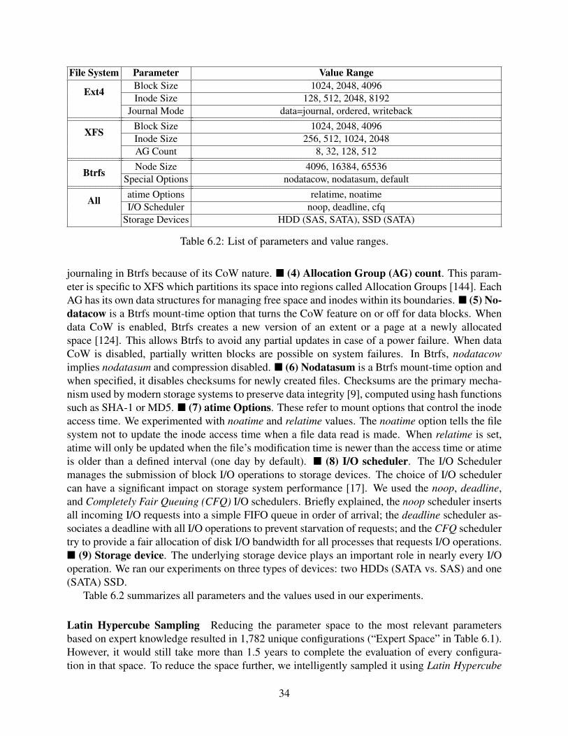
File System Parameter Value Range

Ext4 Block Size 1024, 2048, 4096Inode Size 128, 512, 2048, 8192

Journal Mode data=journal, ordered, writeback

XFS Block Size 1024, 2048, 4096Inode Size 256, 512, 1024, 2048AG Count 8, 32, 128, 512

Btrfs Node Size 4096, 16384, 65536Special Options nodatacow, nodatasum, default

All atime Options relatime, noatimeI/O Scheduler noop, deadline, cfq

Storage Devices HDD (SAS, SATA), SSD (SATA)

Table 6.2: List of parameters and value ranges.

journaling in Btrfs because of its CoW nature. � (4) Allocation Group (AG) count. This param-eter is specific to XFS which partitions its space into regions called Allocation Groups [144]. EachAG has its own data structures for managing free space and inodes within its boundaries. � (5) No-datacow is a Btrfs mount-time option that turns the CoW feature on or off for data blocks. Whendata CoW is enabled, Btrfs creates a new version of an extent or a page at a newly allocatedspace [124]. This allows Btrfs to avoid any partial updates in case of a power failure. When dataCoW is disabled, partially written blocks are possible on system failures. In Btrfs, nodatacowimplies nodatasum and compression disabled. � (6) Nodatasum is a Btrfs mount-time option andwhen specified, it disables checksums for newly created files. Checksums are the primary mecha-nism used by modern storage systems to preserve data integrity [9], computed using hash functionssuch as SHA-1 or MD5. � (7) atime Options. These refer to mount options that control the inodeaccess time. We experimented with noatime and relatime values. The noatime option tells the filesystem not to update the inode access time when a file data read is made. When relatime is set,atime will only be updated when the file’s modification time is newer than the access time or atimeis older than a defined interval (one day by default). � (8) I/O scheduler. The I/O Schedulermanages the submission of block I/O operations to storage devices. The choice of I/O schedulercan have a significant impact on storage system performance [17]. We used the noop, deadline,and Completely Fair Queuing (CFQ) I/O schedulers. Briefly explained, the noop scheduler insertsall incoming I/O requests into a simple FIFO queue in order of arrival; the deadline scheduler as-sociates a deadline with all I/O operations to prevent starvation of requests; and the CFQ schedulertry to provide a fair allocation of disk I/O bandwidth for all processes that requests I/O operations.� (9) Storage device. The underlying storage device plays an important role in nearly every I/Ooperation. We ran our experiments on three types of devices: two HDDs (SATA vs. SAS) and one(SATA) SSD.

Table 6.2 summarizes all parameters and the values used in our experiments.

Latin Hypercube Sampling Reducing the parameter space to the most relevant parametersbased on expert knowledge resulted in 1,782 unique configurations (“Expert Space” in Table 6.1).However, it would still take more than 1.5 years to complete the evaluation of every configura-tion in that space. To reduce the space further, we intelligently sampled it using Latin Hypercube

34

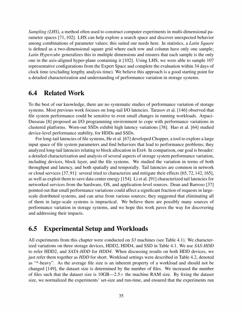
Sampling (LHS), a method often used to construct computer experiments in multi-dimensional pa-rameter spaces [71, 102]. LHS can help explore a search space and discover unexpected behavioramong combinations of parameter values; this suited our needs here. In statistics, a Latin Squareis defined as a two-dimensional square grid where each row and column have only one sample;Latin Hypercube generalizes this to multiple dimensions and ensures that each sample is the onlyone in the axis-aligned hyper-plane containing it [102]. Using LHS, we were able to sample 107representative configurations from the Expert Space and complete the evaluation within 34 days ofclock time (excluding lengthy analysis time). We believe this approach is a good starting point fora detailed characterization and understanding of performance variation in storage systems.

6.4 Related WorkTo the best of our knowledge, there are no systematic studies of performance variation of storagesystems. Most previous work focuses on long-tail I/O latencies. Tarasov et al. [146] observed thatfile system performance could be sensitive to even small changes in running workloads. Arpaci-Dusseau [8] proposed an I/O programming environment to cope with performance variations inclustered platforms. Worn-out SSDs exhibit high latency variations [38]. Hao et al. [64] studieddevice-level performance stability, for HDDs and SSDs.

For long-tail latencies of file systems, He et al. [67] developed Chopper, a tool to explore a largeinput space of file system parameters and find behaviors that lead to performance problems; theyanalyzed long-tail latencies relating to block allocation in Ext4. In comparison, our goal is broader:a detailed characterization and analysis of several aspects of storage system performance variation,including devices, block layer, and the file systems. We studied the variation in terms of boththroughput and latency, and both spatially and temporally. Tail latencies are common in networkor cloud services [37, 91]: several tried to characterize and mitigate their effects [65, 72, 142, 165],as well as exploit them to save data center energy [154]. Li et al. [91] characterized tail latencies fornetworked services from the hardware, OS, and application-level sources. Dean and Barroso [37]pointed out that small performance variations could affect a significant fraction of requests in large-scale distributed systems, and can arise from various sources; they suggested that eliminating allof them in large-scale systems is impractical. We believe there are possibly many sources ofperformance variation in storage systems, and we hope this work paves the way for discoveringand addressing their impacts.

6.5 Experimental Setup and WorkloadsAll experiments from this chapter were conducted on S3 machines (see Table 4.1). We character-ized variations on three storage devices, HDD2, HDD4, and SSD in Table 4.1. We use SAS-HDDto refer HDD2, and SATA-HDD for HDD4. When discussing results on both HDD devices, wejust refer them together as HDD for short. Workload settings were described in Table 4.2, denotedas “*-heavy”. As the average file size is an inherent property of a workload and should not bechanged [149], the dataset size is determined by the number of files. We increased the numberof files such that the dataset size is 10GB—2.5× the machine RAM size. By fixing the datasetsize, we normalized the experiments’ set-size and run-time, and ensured that the experiments run

35

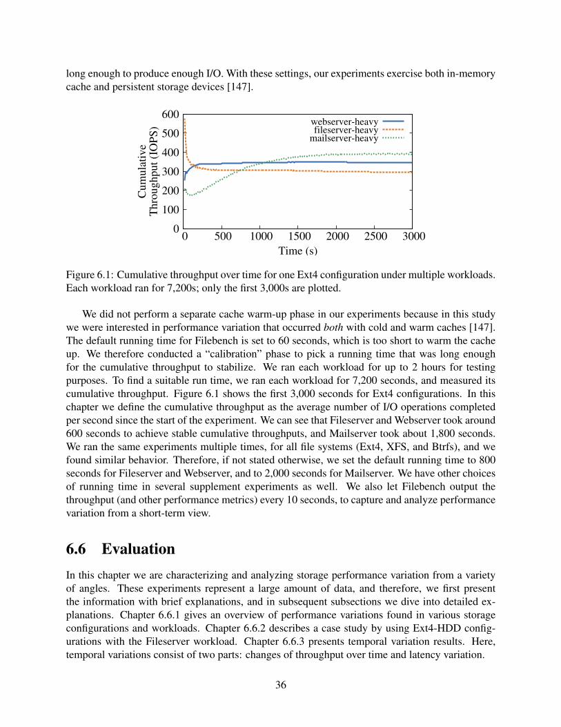
long enough to produce enough I/O. With these settings, our experiments exercise both in-memorycache and persistent storage devices [147].

0

100

200

300

400

500

600

0 500 1000 1500 2000 2500 3000

Cum

ula

tive

Thro

ughput

(IO

PS

)

Time (s)

webserver-heavyfileserver-heavy

mailserver-heavy

Figure 6.1: Cumulative throughput over time for one Ext4 configuration under multiple workloads.Each workload ran for 7,200s; only the first 3,000s are plotted.

We did not perform a separate cache warm-up phase in our experiments because in this studywe were interested in performance variation that occurred both with cold and warm caches [147].The default running time for Filebench is set to 60 seconds, which is too short to warm the cacheup. We therefore conducted a “calibration” phase to pick a running time that was long enoughfor the cumulative throughput to stabilize. We ran each workload for up to 2 hours for testingpurposes. To find a suitable run time, we ran each workload for 7,200 seconds, and measured itscumulative throughput. Figure 6.1 shows the first 3,000 seconds for Ext4 configurations. In thischapter we define the cumulative throughput as the average number of I/O operations completedper second since the start of the experiment. We can see that Fileserver and Webserver took around600 seconds to achieve stable cumulative throughputs, and Mailserver took about 1,800 seconds.We ran the same experiments multiple times, for all file systems (Ext4, XFS, and Btrfs), and wefound similar behavior. Therefore, if not stated otherwise, we set the default running time to 800seconds for Fileserver and Webserver, and to 2,000 seconds for Mailserver. We have other choicesof running time in several supplement experiments as well. We also let Filebench output thethroughput (and other performance metrics) every 10 seconds, to capture and analyze performancevariation from a short-term view.

6.6 EvaluationIn this chapter we are characterizing and analyzing storage performance variation from a varietyof angles. These experiments represent a large amount of data, and therefore, we first presentthe information with brief explanations, and in subsequent subsections we dive into detailed ex-planations. Chapter 6.6.1 gives an overview of performance variations found in various storageconfigurations and workloads. Chapter 6.6.2 describes a case study by using Ext4-HDD config-urations with the Fileserver workload. Chapter 6.6.3 presents temporal variation results. Here,temporal variations consist of two parts: changes of throughput over time and latency variation.

36

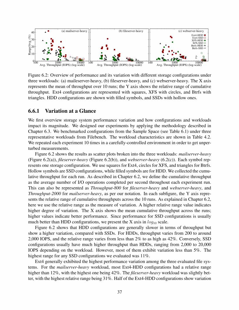
0

10

20

30

40

100 1000 10000

Ran

ge/

Avg. (%

)

Avg. Throughput (IOPS) (log-scale)

(a) mailserver-heavy

100 1000 10000Avg. Throughput (IOPS) (log-scale)

(b) fileserver-heavy

100 1000 10000Avg. Throughput (IOPS) (log-scale)

(c) webserver-heavy

Ext4-HDDExt4-SSD

XFS-HDDXFS-SSD

Btrfs-HDDBtrfs-SSD

Figure 6.2: Overview of performance and its variation with different storage configurations underthree workloads: (a) maileserver-heavy, (b) fileserver-heavy, and (c) webserver-heavy. The X axisrepresents the mean of throughput over 10 runs; the Y axis shows the relative range of cumulativethroughput. Ext4 configurations are represented with squares, XFS with circles, and Btrfs withtriangles. HDD configurations are shown with filled symbols, and SSDs with hollow ones.

6.6.1 Variation at a GlanceWe first overview storage system performance variation and how configurations and workloadsimpact its magnitude. We designed our experiments by applying the methodology described inChapter 6.3. We benchmarked configurations from the Sample Space (see Table 6.1) under threerepresentative workloads from Filebench. The workload characteristics are shown in Table 4.2.We repeated each experiment 10 times in a carefully-controlled environment in order to get unper-turbed measurements.

Figure 6.2 shows the results as scatter plots broken into the three workloads: mailserver-heavy(Figure 6.2(a)), fileserver-heavy (Figure 6.2(b)), and webserver-heavy (6.2(c)). Each symbol rep-resents one storage configuration. We use squares for Ext4, circles for XFS, and triangles for Btrfs.Hollow symbols are SSD configurations, while filled symbols are for HDD. We collected the cumu-lative throughput for each run. As described in Chapter 6.2, we define the cumulative throughputas the average number of I/O operations completed per second throughout each experiment run.This can also be represented as Throughput-800 for fileserver-heavy and webserver-heavy, andThroughput-2000 for mailserver-heavy, as per our notation. In each subfigure, the Y axis repre-sents the relative range of cumulative throughputs across the 10 runs. As explained in Chapter 6.2,here we use the relative range as the measure of variation. A higher relative range value indicateshigher degree of variation. The X axis shows the mean cumulative throughput across the runs;higher values indicate better performance. Since performance for SSD configurations is usuallymuch better than HDD configurations, we present the X axis in log10 scale.

Figure 6.2 shows that HDD configurations are generally slower in terms of throughput butshow a higher variation, compared with SSDs. For HDDs, throughput varies from 200 to around2,000 IOPS, and the relative range varies from less than 2% to as high as 42%. Conversely, SSDconfigurations usually have much higher throughput than HDDs, ranging from 2,000 to 20,000IOPS depending on the workload. However, most of them exhibit variation less than 5%. Thehighest range for any SSD configurations we evaluated was 11%.

Ext4 generally exhibited the highest performance variation among the three evaluated file sys-tems. For the mailserver-heavy workload, most Ext4-HDD configurations had a relative rangehigher than 12%, with the highest one being 42%. The fileserver-heavy workload was slightly bet-ter, with the highest relative range being 31%. Half of the Ext4-HDD configurations show variation

37

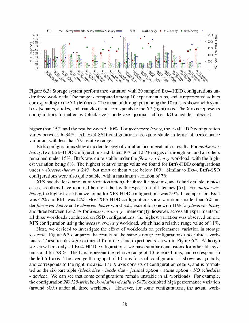
0%

5%

10%

15%

20%

25%

30%

35%

40%

45%

2K-128-journal-

rel-ddln-sata

2K-128-ordered-

rel-cfq-sata

2K-128-w

rback-

rel-ddln-sata

2K-128-journal-

no-cfq-sas

2K-128-journal-

no-cfq-sata

2K-128-ordered-

no-cfq-sas

2K-512-w

rback-

no-ddln-sata

2K-2K

-wrback-

rel-cfq-sas

2K-2K

-ordered-

no-noop-sas

2K-2K

-ordered-

no-cfq-sas

2K-2K

-wrback-

no-noop-sata

4K-128-journal-

no-cfq-sata

4K-128-w

rback-

no-cfq-sas

4K-512-ordered-

rel-noop-sas

4K-512-ordered-

rel-noop-sata

4K-512-w

rback-

rel-noop-sata

4K-512-journal-

no-cfq-sata

4K-512-journal-

no-ddln-sata

4K-2K

-wrback-

rel-cfq-sas

4K-2K

-wrback-

no-noop-sas

0

500

1000

1500

2000

2500

Y1:

Ran

ge/

Av

g.

Y2:

Av

g.

Th

rou

gh

pu

t (I

OP

S)

Y1: mail-heavy file-heavy web-heavy Y2: mail-heavy file-heavy web-heavy

Figure 6.3: Storage system performance variation with 20 sampled Ext4-HDD configurations un-der three workloads. The range is computed among 10 experiment runs, and is represented as barscorresponding to the Y1 (left) axis. The mean of throughput among the 10 runs is shown with sym-bols (squares, circles, and triangles), and corresponds to the Y2 (right) axis. The X axis representsconfigurations formatted by 〈block size - inode size - journal - atime - I/O scheduler - device〉.

higher than 15% and the rest between 5–10%. For webserver-heavy, the Ext4-HDD configurationvaries between 6–34%. All Ext4-SSD configurations are quite stable in terms of performancevariation, with less than 5% relative range.

Btrfs configurations show a moderate level of variation in our evaluation results. For mailserver-heavy, two Btrfs-HDD configurations exhibited 40% and 28% ranges of throughput, and all othersremained under 15%. Btrfs was quite stable under the fileserver-heavy workload, with the high-est variation being 8%. The highest relative range value we found for Btrfs-HDD configurationsunder webserver-heavy is 24%, but most of them were below 10%. Similar to Ext4, Btrfs-SSDconfigurations were also quite stable, with a maximum variation of 7%.

XFS had the least amount of variation among the three file systems, and is fairly stable in mostcases, as others have reported before, albeit with respect to tail latencies [67]. For mailserver-heavy, the highest variation we found for XFS-HDD configurations was 25%. In comparison, Ext4was 42% and Btrfs was 40%. Most XFS-HDD configurations show variation smaller than 5% un-der fileserver-heavy and webserver-heavy workloads, except for one with 11% for fileserver-heavyand three between 12–23% for webserver-heavy. Interestingly, however, across all experiments forall three workloads conducted on SSD configurations, the highest variation was observed on oneXFS configuration using the webserver-heavy workload, which had a relative range value of 11%.

Next, we decided to investigate the effect of workloads on performance variation in storagesystems. Figure 6.3 compares the results of the same storage configurations under three work-loads. These results were extracted from the same experiments shown in Figure 6.2. Althoughwe show here only all Ext4-HDD configurations, we have similar conclusions for other file sys-tems and for SSDs. The bars represent the relative range of 10 repeated runs, and correspond tothe left Y1 axis. The average throughput of 10 runs for each configuration is shown as symbols,and corresponds to the right Y2 axis. The X axis consists of configuration details, and is format-ted as the six-part tuple 〈block size - inode size - journal option - atime option - I/O scheduler- device〉. We can see that some configurations remain unstable in all workloads. For example,the configuration 2K-128-writeback-relatime-deadline-SATA exhibited high performance variation(around 30%) under all three workloads. However, for some configurations, the actual work-

38

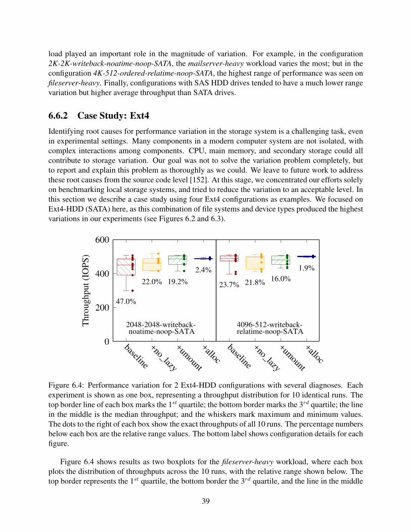
load played an important role in the magnitude of variation. For example, in the configuration2K-2K-writeback-noatime-noop-SATA, the mailserver-heavy workload varies the most; but in theconfiguration 4K-512-ordered-relatime-noop-SATA, the highest range of performance was seen onfileserver-heavy. Finally, configurations with SAS HDD drives tended to have a much lower rangevariation but higher average throughput than SATA drives.

6.6.2 Case Study: Ext4Identifying root causes for performance variation in the storage system is a challenging task, evenin experimental settings. Many components in a modern computer system are not isolated, withcomplex interactions among components. CPU, main memory, and secondary storage could allcontribute to storage variation. Our goal was not to solve the variation problem completely, butto report and explain this problem as thoroughly as we could. We leave to future work to addressthese root causes from the source code level [152]. At this stage, we concentrated our efforts solelyon benchmarking local storage systems, and tried to reduce the variation to an acceptable level. Inthis section we describe a case study using four Ext4 configurations as examples. We focused onExt4-HDD (SATA) here, as this combination of file systems and device types produced the highestvariations in our experiments (see Figures 6.2 and 6.3).

0

200

400

600

baseline

+no_lazy

+umount

+alloc

baseline

+no_lazy

+umount

+alloc

2048-2048-writeback-noatime-noop-SATA

4096-512-writeback-relatime-noop-SATA

Th

rou

gh

pu

t (I

OP

S)

47.0%

22.0% 19.2%

2.4%

23.7% 21.8%16.0%

1.9%

Figure 6.4: Performance variation for 2 Ext4-HDD configurations with several diagnoses. Eachexperiment is shown as one box, representing a throughput distribution for 10 identical runs. Thetop border line of each box marks the 1st quartile; the bottom border marks the 3rd quartile; the linein the middle is the median throughput; and the whiskers mark maximum and minimum values.The dots to the right of each box show the exact throughputs of all 10 runs. The percentage numbersbelow each box are the relative range values. The bottom label shows configuration details for eachfigure.

Figure 6.4 shows results as two boxplots for the fileserver-heavy workload, where each boxplots the distribution of throughputs across the 10 runs, with the relative range shown below. Thetop border represents the 1st quartile, the bottom border the 3rd quartile, and the line in the middle

39

is the median value. Whiskers show the maximum and minimum throughputs. We also plotted onedot for the throughput of each run, overlapping with the boxes but shifted to the right for easierviewing. The X axis represents the relative improvements that we applied based on our successiveinvestigations and uncovering of root causes of performance variation, while the Y axis shows thecumulative throughput for each experiment run. Note that the improvement label is prefixed with a“+” sign, meaning that an additional feature was added to the previous configuration, cumulatively.For example, +umount actually indicates baseline + no lazy + umount. We also added labels onthe bottom of each subfigure showing the configuration details, formatted as 〈block size - inodesize - journal option - atime option - I/O scheduler - device〉.

After addressing all causes we found, we were able to reduce the relative range of throughputin these configurations from as high as 47% to around 2%. In the rest of this section, we detaileach root cause and how we addressed it.

Baseline The first box for each subfigure in Figure 6.4 represents our original experiment setting,labeled baseline. In this setting, before each experimental run, we format and mount the filesystem with the targeted configuration. Filebench then creates the dataset on the mounted filesystem. After the dataset is created, Filebench issues the sync command to flush all dirty dataand metadata to the underlying device (here, SATA HDD); Filebench then issues an echo 3 >/proc/sys/vm/drop caches command, to evict non-dirty data and metadata from the page cache.Then, Filebench runs the Fileserver workload for a pre-defined amount of time (see Table 4.2). Forthis baseline setting, both Ext4-HDD configurations show high variation in terms of throughput,with range values of 47% (left) and 24% (right).

Lazy initialization The first contributor to performance variation that we identified in Ext4-HDD configurations is related to the lazy initialization mechanism in Ext4. By default, Ext4does not immediately initialize the complete inode table. Instead, it gradually initializes it in thebackground when the created file system is first mounted, using a kernel thread called ext4lazyinit.After the initialization is done, the thread is destroyed. This feature speeds up the formattingprocess significantly, but also causes interference with the running workload. By disabling it duringformat time, we reduced the range of throughput from 47% to 22% for Configuration 2048-2048-writeback-noatime-noop-SATA. This improvement is labelled +no lazy in Figure 6.4.

Sync then umount In Linux, when sync is called, it only guarantees to schedule the dirty blocksfor writing: there is often a delay until all blocks are actually written to stable media [116, 145].Therefore, instead of calling sync, we umount the file system each time after finishing creating thedataset and then mount it back, which is labelled as +umount in Figure 6.4. After applying this,both Ext4-HDD configurations exhibited even lower variation than the previous setting (disablinglazy initialization only).

Block allocation and layout After applying the above improvements, both configurations stillexhibited higher than 16% variations, which could be unacceptable in settings that require morepredictable performance. This inspired us to try an even more strictly-controlled set of exper-iments. In the baseline experiments, by default we re-created the file system before each runand then Filebench created the dataset. We assumed that this approach would result in identical

40

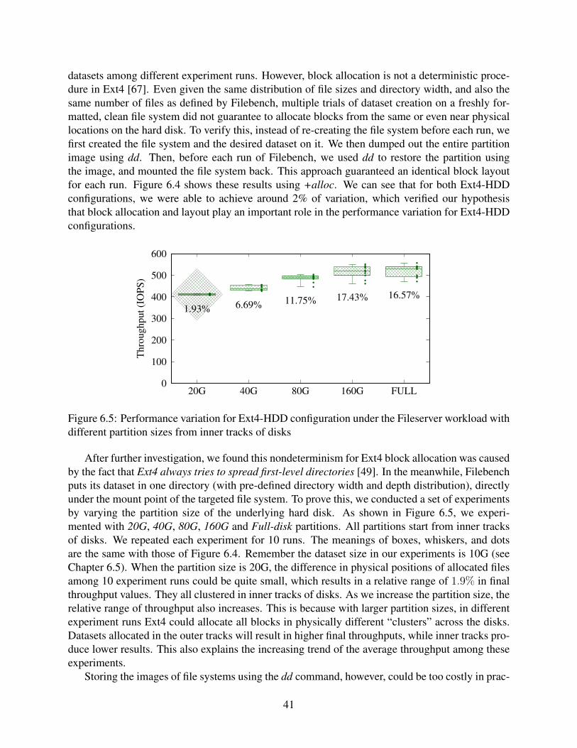
datasets among different experiment runs. However, block allocation is not a deterministic proce-dure in Ext4 [67]. Even given the same distribution of file sizes and directory width, and also thesame number of files as defined by Filebench, multiple trials of dataset creation on a freshly for-matted, clean file system did not guarantee to allocate blocks from the same or even near physicallocations on the hard disk. To verify this, instead of re-creating the file system before each run, wefirst created the file system and the desired dataset on it. We then dumped out the entire partitionimage using dd. Then, before each run of Filebench, we used dd to restore the partition usingthe image, and mounted the file system back. This approach guaranteed an identical block layoutfor each run. Figure 6.4 shows these results using +alloc. We can see that for both Ext4-HDDconfigurations, we were able to achieve around 2% of variation, which verified our hypothesisthat block allocation and layout play an important role in the performance variation for Ext4-HDDconfigurations.

0

100

200

300

400

500

600

20G 40G 80G 160G FULL

Th

rou

gh

pu

t (I

OP

S)

1.93% 6.69% 11.75% 17.43% 16.57%

Figure 6.5: Performance variation for Ext4-HDD configuration under the Fileserver workload withdifferent partition sizes from inner tracks of disks

After further investigation, we found this nondeterminism for Ext4 block allocation was causedby the fact that Ext4 always tries to spread first-level directories [49]. In the meanwhile, Filebenchputs its dataset in one directory (with pre-defined directory width and depth distribution), directlyunder the mount point of the targeted file system. To prove this, we conducted a set of experimentsby varying the partition size of the underlying hard disk. As shown in Figure 6.5, we experi-mented with 20G, 40G, 80G, 160G and Full-disk partitions. All partitions start from inner tracksof disks. We repeated each experiment for 10 runs. The meanings of boxes, whiskers, and dotsare the same with those of Figure 6.4. Remember the dataset size in our experiments is 10G (seeChapter 6.5). When the partition size is 20G, the difference in physical positions of allocated filesamong 10 experiment runs could be quite small, which results in a relative range of 1.9% in finalthroughput values. They all clustered in inner tracks of disks. As we increase the partition size, therelative range of throughput also increases. This is because with larger partition sizes, in differentexperiment runs Ext4 could allocate all blocks in physically different “clusters” across the disks.Datasets allocated in the outer tracks will result in higher final throughputs, while inner tracks pro-duce lower results. This also explains the increasing trend of the average throughput among theseexperiments.

Storing the images of file systems using the dd command, however, could be too costly in prac-

41

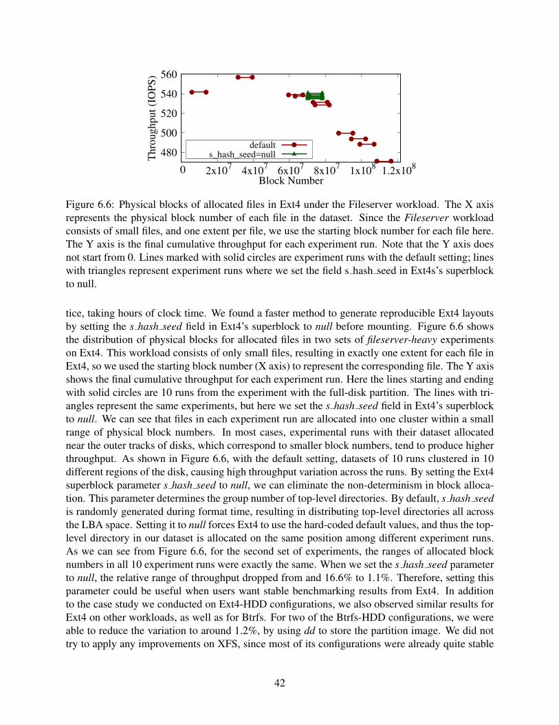
480

500

520

540

560

0 2x107

4x107

6x107

8x107

1x108

1.2x108

Th

rou

gh

pu

t (I

OP

S)

Block Number

defaults_hash_seed=null

Figure 6.6: Physical blocks of allocated files in Ext4 under the Fileserver workload. The X axisrepresents the physical block number of each file in the dataset. Since the Fileserver workloadconsists of small files, and one extent per file, we use the starting block number for each file here.The Y axis is the final cumulative throughput for each experiment run. Note that the Y axis doesnot start from 0. Lines marked with solid circles are experiment runs with the default setting; lineswith triangles represent experiment runs where we set the field s hash seed in Ext4s’s superblockto null.

tice, taking hours of clock time. We found a faster method to generate reproducible Ext4 layoutsby setting the s hash seed field in Ext4’s superblock to null before mounting. Figure 6.6 showsthe distribution of physical blocks for allocated files in two sets of fileserver-heavy experimentson Ext4. This workload consists of only small files, resulting in exactly one extent for each file inExt4, so we used the starting block number (X axis) to represent the corresponding file. The Y axisshows the final cumulative throughput for each experiment run. Here the lines starting and endingwith solid circles are 10 runs from the experiment with the full-disk partition. The lines with tri-angles represent the same experiments, but here we set the s hash seed field in Ext4’s superblockto null. We can see that files in each experiment run are allocated into one cluster within a smallrange of physical block numbers. In most cases, experimental runs with their dataset allocatednear the outer tracks of disks, which correspond to smaller block numbers, tend to produce higherthroughput. As shown in Figure 6.6, with the default setting, datasets of 10 runs clustered in 10different regions of the disk, causing high throughput variation across the runs. By setting the Ext4superblock parameter s hash seed to null, we can eliminate the non-determinism in block alloca-tion. This parameter determines the group number of top-level directories. By default, s hash seedis randomly generated during format time, resulting in distributing top-level directories all acrossthe LBA space. Setting it to null forces Ext4 to use the hard-coded default values, and thus the top-level directory in our dataset is allocated on the same position among different experiment runs.As we can see from Figure 6.6, for the second set of experiments, the ranges of allocated blocknumbers in all 10 experiment runs were exactly the same. When we set the s hash seed parameterto null, the relative range of throughput dropped from and 16.6% to 1.1%. Therefore, setting thisparameter could be useful when users want stable benchmarking results from Ext4. In additionto the case study we conducted on Ext4-HDD configurations, we also observed similar results forExt4 on other workloads, as well as for Btrfs. For two of the Btrfs-HDD configurations, we wereable to reduce the variation to around 1.2%, by using dd to store the partition image. We did nottry to apply any improvements on XFS, since most of its configurations were already quite stable

42

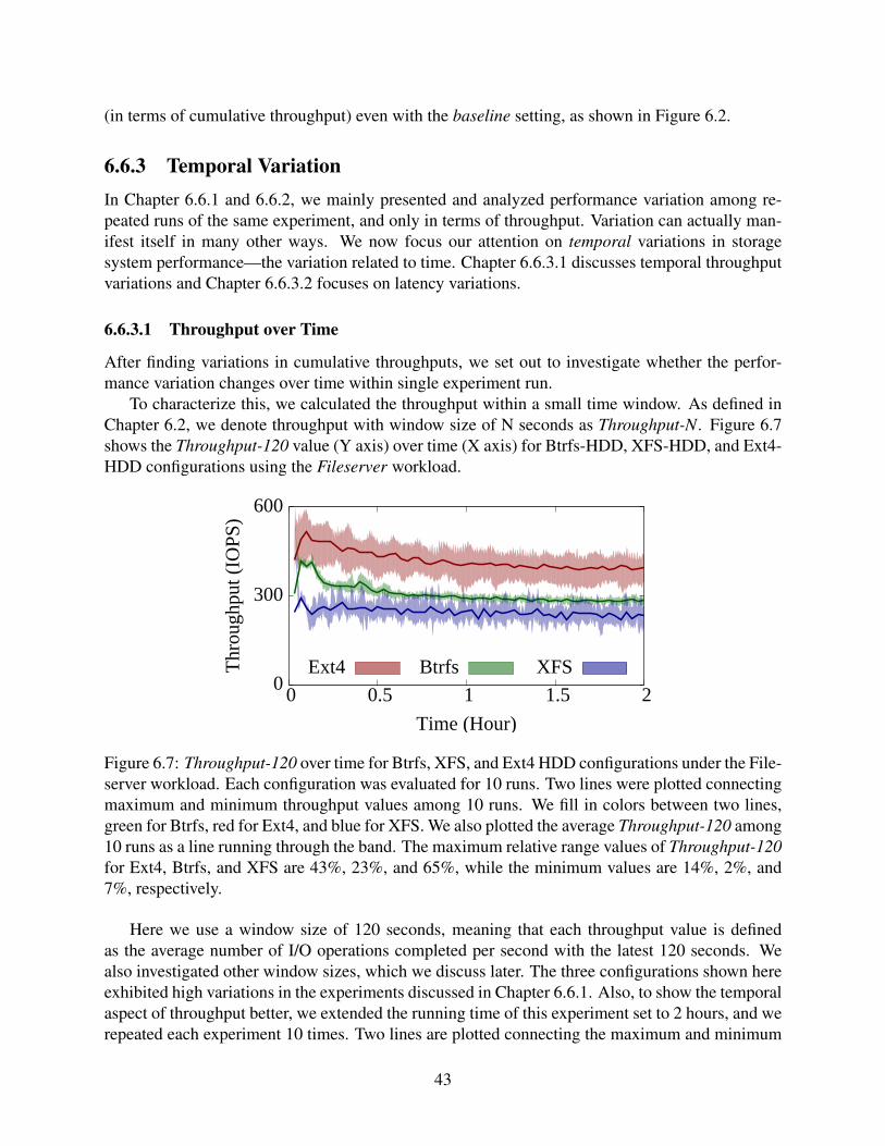
(in terms of cumulative throughput) even with the baseline setting, as shown in Figure 6.2.

6.6.3 Temporal VariationIn Chapter 6.6.1 and 6.6.2, we mainly presented and analyzed performance variation among re-peated runs of the same experiment, and only in terms of throughput. Variation can actually man-ifest itself in many other ways. We now focus our attention on temporal variations in storagesystem performance—the variation related to time. Chapter 6.6.3.1 discusses temporal throughputvariations and Chapter 6.6.3.2 focuses on latency variations.

6.6.3.1 Throughput over Time

After finding variations in cumulative throughputs, we set out to investigate whether the perfor-mance variation changes over time within single experiment run.

To characterize this, we calculated the throughput within a small time window. As defined inChapter 6.2, we denote throughput with window size of N seconds as Throughput-N. Figure 6.7shows the Throughput-120 value (Y axis) over time (X axis) for Btrfs-HDD, XFS-HDD, and Ext4-HDD configurations using the Fileserver workload.

0

300

600

0 0.5 1 1.5 2

Thro

ughp

ut (I

OPS

)

Time (Hour)

Ext4 Btrfs XFS

Figure 6.7: Throughput-120 over time for Btrfs, XFS, and Ext4 HDD configurations under the File-server workload. Each configuration was evaluated for 10 runs. Two lines were plotted connectingmaximum and minimum throughput values among 10 runs. We fill in colors between two lines,green for Btrfs, red for Ext4, and blue for XFS. We also plotted the average Throughput-120 among10 runs as a line running through the band. The maximum relative range values of Throughput-120for Ext4, Btrfs, and XFS are 43%, 23%, and 65%, while the minimum values are 14%, 2%, and7%, respectively.

Here we use a window size of 120 seconds, meaning that each throughput value is definedas the average number of I/O operations completed per second with the latest 120 seconds. Wealso investigated other window sizes, which we discuss later. The three configurations shown hereexhibited high variations in the experiments discussed in Chapter 6.6.1. Also, to show the temporalaspect of throughput better, we extended the running time of this experiment set to 2 hours, and werepeated each experiment 10 times. Two lines are plotted connecting the maximum and minimum

43

throughput values among 10 runs. We fill in colors between two lines, this producing a color band:green for Btrfs, red for Ext4, and blue for XFS. The line in the middle of each band is plotted byconnecting the average Throughput-120 value among 10 runs. We observed in Figure 6.2(b) thatfor the fileserver-heavy workload, Ext4-HDD configurations generally exhibited higher variationsthan XFS-HDD or Btrfs-HDD configurations in terms of final cumulative throughput. However,when it comes to Throughput-120 values, Figure 6.7 leads to some different conclusions. TheExt4-HDD configuration still exhibited high variation in terms of short-term throughout across the2 hours of experiment time, while the Btrfs-HDD configuration is much more stable. Surprisingly,the XFS-HDD configuration has higher than 30% relative range of Throughput-120 values for mostof the experiment time, while its range for cumulative throughput is around 2%. This suggests thatXFS-HDD configurations might exhibit high variations with shorter time windows, but producesmore stable results in longer windows. It also indicates that the choice of window sizes matterswhen discussing performance variations.

We can see from the three average lines in Figure 6.7 that performance variation exists evenwithin one single run—the short-term throughput varies as the experiment proceeds. For mostexperiments, no matter what the file system type is, performance starts slow and climbs up quicklyin the beginning phase of experiments. This is because initially the application is reading cold dataand metadata from physical devices into the caches; once cached, performance improves. Also, forsome period of time, dirty data is kept in the cache and not yet flushed to stable media, delayingany impending slow writes. After an initial peak, performance begins to drop rapidly and thendeclines steadily. This is because the read performance already reached its peak and cached dirtydata begins to be flushed out to slower media. Around several minutes in, performance begins tostabilize, as we see the throughput lines flatten.

The unexpected difference in variations for short-term and cumulative throughput of XFS-HDDconfigurations lead us to investigate the effects of the time window size on performance variations.We calculated the relative range of throughput with different window sizes for all configurationswithin each file system type. We present the CDFs of these range values in Figure 6.8. Forexample, we conducted experiments on 39 Btrfs configurations. With a window size of 60 secondsand total running time of 800 seconds, the corresponding CDF for Btrfs is based on 39× 800

60= 507

relative range values. We can see that Ext4’s unstable configurations are largely unaffected by thewindow size. Even with Throughput-400, around 20% of Ext4 configurations produce higherthan 20% variation in terms of throughput. Conversely, the range values for Btrfs and XFS aremore sensitive to the choice of window size. For XFS, around 40% of the relative range valuesfor Throughput-60 are higher than 20%, whereas for Throughput-400, nearly all XFS values fallbelow 20%. This aligns with our early conclusions in Chapter 6.6.1 that XFS configurations arerelatively stable in terms of cumulative throughput, which is indeed calculated based on a windowsize of 800 seconds; whereas XFS showed the worst relative range for Throughput-60, it stabilizedquickly with widening window sizes, eventually beating Ext4 and Btrfs.

All the above observations are based on the throughput within a certain window size. Anotherapproach is to characterize the instant throughput within an even shorter period of time. Figure 6.9shows the instantaneous throughput over time for various configurations under the fileserver-heavyworkload. We collected and calculated the throughput every 10 seconds. Therefore we define in-stantaneous throughput as the average number of I/O operations completed in the past 10 seconds.This is actually Throughput-10 in our notation. We normalize this by dividing each value by themaximum instantaneous throughput value for each run, to compare the variation across multiple

44

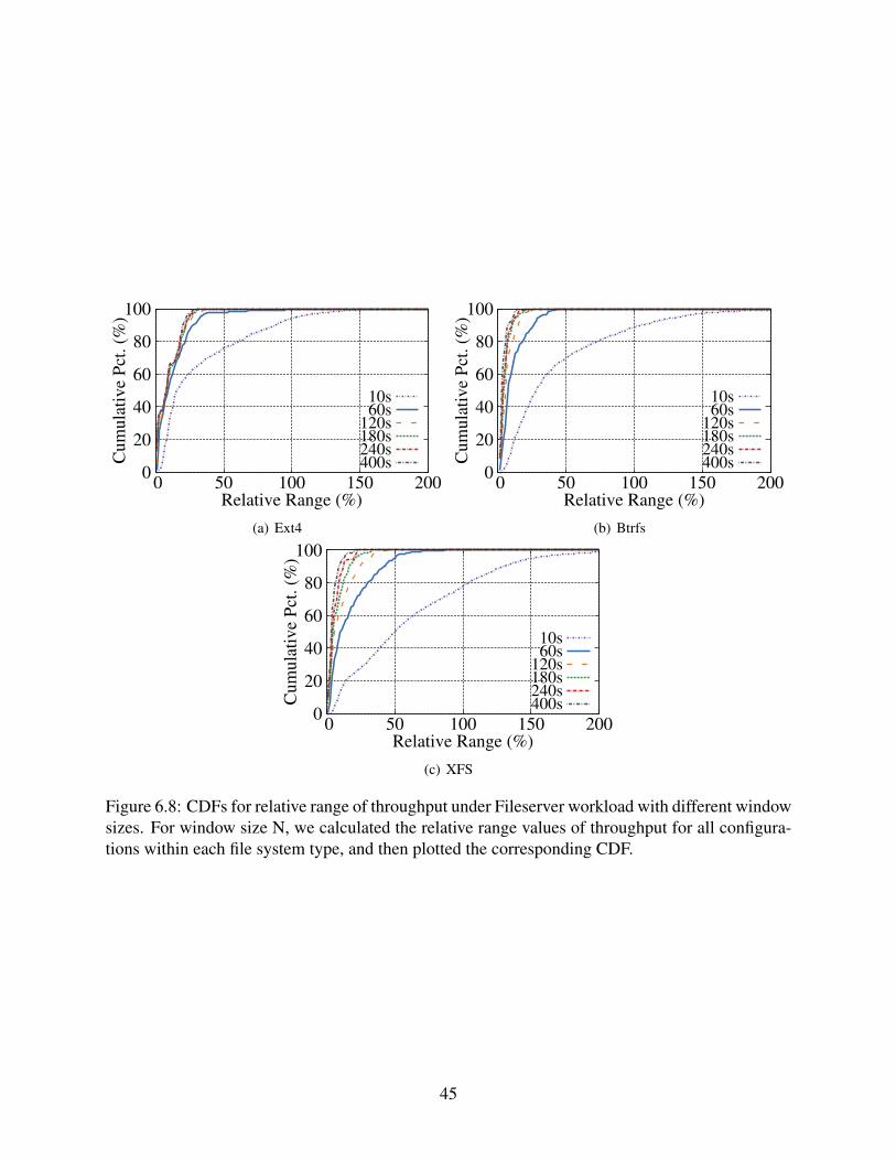
0

20

40

60

80

100

0 50 100 150 200

Cum

ula

tive

Pct

. (%

)

Relative Range (%)

10s60s

120s180s240s400s

(a) Ext4

0

20

40

60

80

100

0 50 100 150 200

Cum

ula

tive

Pct

. (%

)

Relative Range (%)

10s60s

120s180s240s400s

(b) Btrfs

0

20

40

60

80

100

0 50 100 150 200

Cum

ula

tiv

e P

ct. (%

)

Relative Range (%)

10s60s

120s180s240s400s

(c) XFS

Figure 6.8: CDFs for relative range of throughput under Fileserver workload with different windowsizes. For window size N, we calculated the relative range values of throughput for all configura-tions within each file system type, and then plotted the corresponding CDF.

45

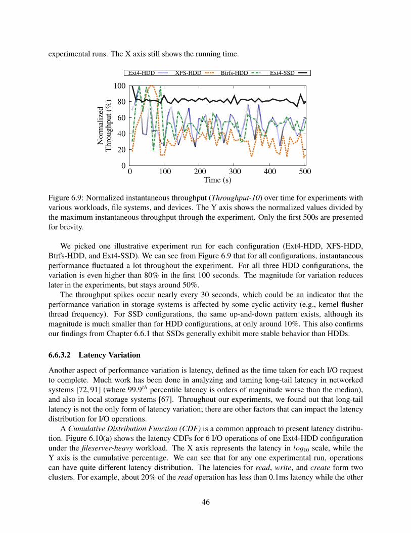
experimental runs. The X axis still shows the running time.

0

20

40

60

80

100

0 100 200 300 400 500

No

rmal

ized

Th

rou

gh

pu

t (%

)

Time (s)

Ext4-HDD XFS-HDD Btrfs-HDD Ext4-SSD

Figure 6.9: Normalized instantaneous throughput (Throughput-10) over time for experiments withvarious workloads, file systems, and devices. The Y axis shows the normalized values divided bythe maximum instantaneous throughput through the experiment. Only the first 500s are presentedfor brevity.

We picked one illustrative experiment run for each configuration (Ext4-HDD, XFS-HDD,Btrfs-HDD, and Ext4-SSD). We can see from Figure 6.9 that for all configurations, instantaneousperformance fluctuated a lot throughout the experiment. For all three HDD configurations, thevariation is even higher than 80% in the first 100 seconds. The magnitude for variation reduceslater in the experiments, but stays around 50%.

The throughput spikes occur nearly every 30 seconds, which could be an indicator that theperformance variation in storage systems is affected by some cyclic activity (e.g., kernel flusherthread frequency). For SSD configurations, the same up-and-down pattern exists, although itsmagnitude is much smaller than for HDD configurations, at only around 10%. This also confirmsour findings from Chapter 6.6.1 that SSDs generally exhibit more stable behavior than HDDs.

6.6.3.2 Latency Variation

Another aspect of performance variation is latency, defined as the time taken for each I/O requestto complete. Much work has been done in analyzing and taming long-tail latency in networkedsystems [72, 91] (where 99.9th percentile latency is orders of magnitude worse than the median),and also in local storage systems [67]. Throughout our experiments, we found out that long-taillatency is not the only form of latency variation; there are other factors that can impact the latencydistribution for I/O operations.

A Cumulative Distribution Function (CDF) is a common approach to present latency distribu-tion. Figure 6.10(a) shows the latency CDFs for 6 I/O operations of one Ext4-HDD configurationunder the fileserver-heavy workload. The X axis represents the latency in log10 scale, while theY axis is the cumulative percentage. We can see that for any one experimental run, operationscan have quite different latency distribution. The latencies for read, write, and create form twoclusters. For example, about 20% of the read operation has less than 0.1ms latency while the other

46

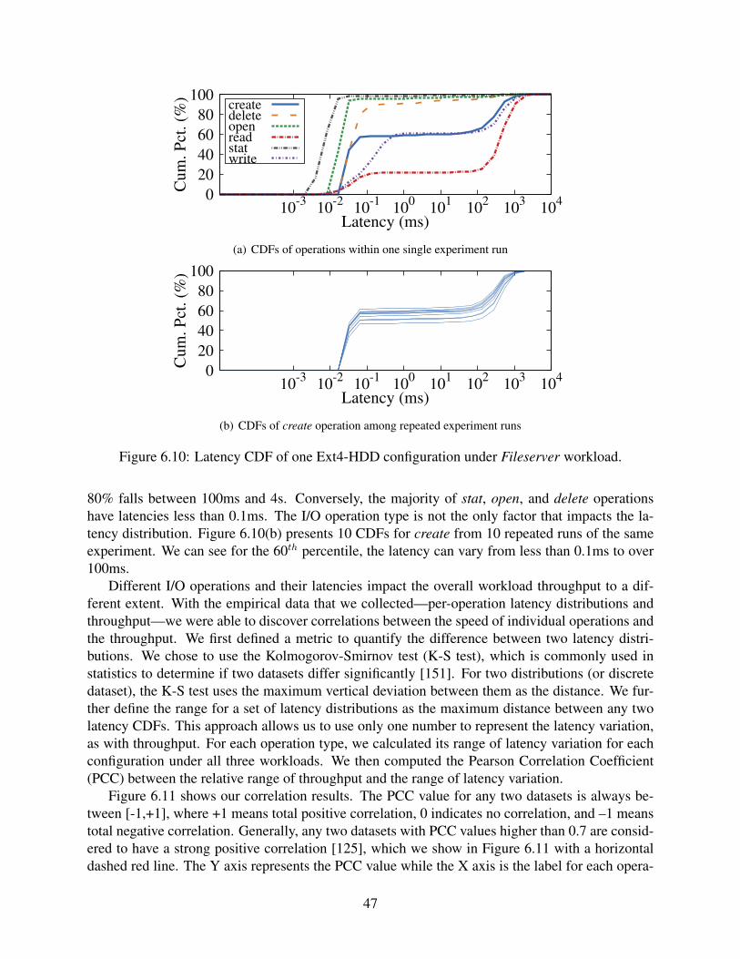
0

20

40

60

80

100

10-3

10-2

10-1

100

101

102

103

104

Cu

m.

Pct

. (%

)

Latency (ms)

create delete open read stat write

(a) CDFs of operations within one single experiment run

0

20

40

60

80

100

10-3

10-2

10-1

100

101

102

103

104

Cu

m.

Pct

. (%

)

Latency (ms)

(b) CDFs of create operation among repeated experiment runs

Figure 6.10: Latency CDF of one Ext4-HDD configuration under Fileserver workload.

80% falls between 100ms and 4s. Conversely, the majority of stat, open, and delete operationshave latencies less than 0.1ms. The I/O operation type is not the only factor that impacts the la-tency distribution. Figure 6.10(b) presents 10 CDFs for create from 10 repeated runs of the sameexperiment. We can see for the 60th percentile, the latency can vary from less than 0.1ms to over100ms.

Different I/O operations and their latencies impact the overall workload throughput to a dif-ferent extent. With the empirical data that we collected—per-operation latency distributions andthroughput—we were able to discover correlations between the speed of individual operations andthe throughput. We first defined a metric to quantify the difference between two latency distri-butions. We chose to use the Kolmogorov-Smirnov test (K-S test), which is commonly used instatistics to determine if two datasets differ significantly [151]. For two distributions (or discretedataset), the K-S test uses the maximum vertical deviation between them as the distance. We fur-ther define the range for a set of latency distributions as the maximum distance between any twolatency CDFs. This approach allows us to use only one number to represent the latency variation,as with throughput. For each operation type, we calculated its range of latency variation for eachconfiguration under all three workloads. We then computed the Pearson Correlation Coefficient(PCC) between the relative range of throughput and the range of latency variation.

Figure 6.11 shows our correlation results. The PCC value for any two datasets is always be-tween [-1,+1], where +1 means total positive correlation, 0 indicates no correlation, and –1 meanstotal negative correlation. Generally, any two datasets with PCC values higher than 0.7 are consid-ered to have a strong positive correlation [125], which we show in Figure 6.11 with a horizontaldashed red line. The Y axis represents the PCC value while the X axis is the label for each opera-

47

0

0.2

0.4

0.6

0.8

1

create delete fsync open read write create

delete

open

read

stat

write

open

read

write

Pea

rso

n C

orr

elat

ion

Co

effi

cien

t (P

CC

) mail-heavy file-heavy web-heavy

Ext4 XFS Btrfs

Figure 6.11: Pearson Correlation Coefficient (PCC) between throughput range and operation types,for three workloads and three file systems. The horizontal dashed red line at Y=0.7 marks the pointabove which a strong correlation is often considered to exist.

tion. We separate workloads with vertical solid lines. As most SSD configurations are quite stablein terms of performance, we only considered HDD configurations here. For Ext4 configurations,open and read have the highest PCC values on both mailserver-heavy and webserver-heavy work-loads; however, on fileserver-heavy, open and stat have the strongest correlation. These operationscould possibly be the main contributors to performance variation on Ext4-HDD configurations un-der each workload; such operations would represent the first ones one might tackle in the future tohelp stabilize Ext4’s performance on HDD. In comparison, write has a PCC value of only around0.2, which indicates that it may not contribute much to the performance variation. Most operationsshow PCC values larger than 0.4, which suggest weak correlation. This is possibly because I/Ooperations are not completely independent with each other in storage systems.

For the same workload, different file systems exhibit different correlations. For example, un-der the webserver-heavy workload, Ext4 show strong correlation on both read and open; but forXFS, read shows a stronger correlation than open and write. For Btrfs, no operation had a strongcorrelation with the range of throughput, with only read showing a moderate level of correlation.

Although such correlations do not always imply direct causality, we still feel that this correla-tion analysis sheds light on how each operation type might contribute to the overall performancevariation in storage systems.

48

Chapter 7

A Practical Auto-Tuning Framework forStorage

7.1 MotivationsDespite some promising results in applying black-box optimization techniques for auto-tuningstorage systems, we believe these techniques still lack several critical features to achieve practical,real-time auto-tuning. Our own experiments demonstrate that auto-tuning sometimes can be slowin finding near-optimal configurations, especially when the evaluation of even a single configura-tion takes long time (e.g., due to slow I/O). Moreover, there is no implicit mechanism to stop thesearch when it reaches a sufficiently good configuration (and restart it later on as needed). Littleis known on how to initialize the search and give it a good starting point. There is no accountingfor the cost of moving from one configuration to another, which is critically important in someproduction settings.

In this proposal we propose to investigate and develop a more intelligent and practical auto-tuning framework, intended to dynamically optimize storage systems. We are exploring techniquesthat add vital missing features from existing optimization methods:

• A criteria when the optimization algorithm should stop searching, having reached a “goodenough” system configuration.

• A similar criteria when the search algorithm should be restarted, useful when the environ-ment conditions (e.g., workload) have changed enough to take the system off of its optimalpoint.

• A workload modeller, which can extract features from system collected metrics and charac-terize the running workload based on them. This is useful in determining when to restart theauto-tuning process and how to “transfer” evaluation results from one workload to another.

• A mechanism to pick an initial set of search space locations, as well as re-initialize thesearch space after restarting a search—which we have found to have a big impact on theefficacy of any search [23, 43].

49

• A penalty function to assign a (weighted) cost to any new configuration based on the currentsystem state, to account for costly configuration changes (e.g., a simple run-time changeableparameter vs. one that requires a system reboot and some downtime).

We will describe some preliminary results exploring these proposed ideas in this chapter, anddiscuss how these components could help us achieve the goal of auto-tuning storage systems inreal-time.

7.2 Problem StatementResults from Chapter 5 show that several popular black-box optimization methods were all able togradually find better configurations; GA and BO successfully found near-optimal configurations.However, our preliminary results also indicate some limitations when simply applying these tra-ditional black-box optimization. For example, in Figure 5.2 after around 3.5 hours, GA alreadyfound a near-optimal configuration, but it spent a lot of additional rounds and resources, yet notimproving overall performance much if at all; Moreover, Figure 2.2 and Table 5.1 showed thatstorage evaluation results depend heavily on the hardware and running workloads. Our previouswork reported similar observations [24, 132]. Therefore, our auto-tuning framework also needs toreact to environment changes (e.g., hardware, workload). In Figure 5.2, SA got stuck in a con-figuration with throughput value of less than 18K IOps. More experiments we conducted suggestthat the quality of initialization has a large effect on the convergence time and final optimizationresults. Lastly, our preliminary experiments assume that all configurations have identical cost: thatmoving from one configuration to another has the same (low) cost. For many storage systems,however, it is not true: for example, changing the block size of a file system may require costly andtime-consuming reformat and data migration.

7.3 Proposed Auto-Tuning FrameworkTo address the limitations discussed in Chapter 7.2, we propose our enhanced auto-tuning frame-work, as shown in Figure 7.1. It consists of 6 components.

• Monitor, which collects and processes system metrics for other components’ use.

• Workload Modeler, which utilizes metrics collected by the Monitor, to identify a runningworkload on the current system.

• Optimizer, which includes the core auto-tuning algorithm with newly added features, fur-ther detailed in §7.3.2. It calculates the optimization objective for the current system con-figuration, based on metrics collected by the Monitor. Our framework is general enough tooptimize for any objective that can be quantitatively measured. Examples are I/O through-put or latency, energy consumption, or even an economic cost function comprising multiplemetrics [97, 141].

• Controller, which is responsible for changing the system settings based on the configurationpicked by the Optimizer.

50

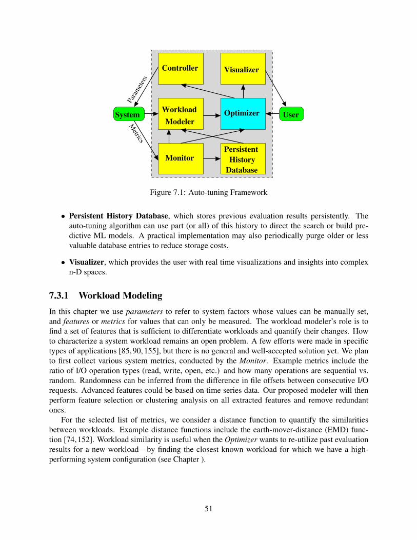
Monitor

Modeler

Workload Optimizer

Visualizer

UserSystem

Para

mete

rs

Metric

s

History

Controller

Database

Persistent

Figure 7.1: Auto-tuning Framework

• Persistent History Database, which stores previous evaluation results persistently. Theauto-tuning algorithm can use part (or all) of this history to direct the search or build pre-dictive ML models. A practical implementation may also periodically purge older or lessvaluable database entries to reduce storage costs.

• Visualizer, which provides the user with real time visualizations and insights into complexn-D spaces.

7.3.1 Workload ModelingIn this chapter we use parameters to refer to system factors whose values can be manually set,and features or metrics for values that can only be measured. The workload modeler’s role is tofind a set of features that is sufficient to differentiate workloads and quantify their changes. Howto characterize a system workload remains an open problem. A few efforts were made in specifictypes of applications [85, 90, 155], but there is no general and well-accepted solution yet. We planto first collect various system metrics, conducted by the Monitor. Example metrics include theratio of I/O operation types (read, write, open, etc.) and how many operations are sequential vs.random. Randomness can be inferred from the difference in file offsets between consecutive I/Orequests. Advanced features could be based on time series data. Our proposed modeler will thenperform feature selection or clustering analysis on all extracted features and remove redundantones.

For the selected list of metrics, we consider a distance function to quantify the similaritiesbetween workloads. Example distance functions include the earth-mover-distance (EMD) func-tion [74,152]. Workload similarity is useful when the Optimizer wants to re-utilize past evaluationresults for a new workload—by finding the closest known workload for which we have a high-performing system configuration (see Chapter ).

51

Fitness

Yes

Start

Evaluate New

Population

Yes

No

No

CrossoverMutationStop?

ElitismML−aided Penalty

ML

MLPenalty

Restart?

InitializePopulation

Selection

Selection

ML

Figure 7.2: Work flow for an enhanced Optimizer (GA).

7.3.2 OptimizerOur proposed Optimizer is designed to address the issues observed in our preliminary experiments.Here we use GA as a case study explaining how it works, but all the new components are applicableto other black-box optimization algorithms as well. As shown in Figure 7.2, white boxes representGA’s original optimization loop components and blue ones relate to GA’s selection process; pinkones are new components in our hybrid optimization algorithm; and green ones show new, ML-aided components.

7.3.3 (Re-)InitializationAs discussed in Chapter 7.2, the quality of initialization has a large impact on the convergence timeand final results of optimization. Much work have been done on proposing and analyzing differ-ent initialization methods for various optimization algorithms [54, 63, 136]. We are investigatingthe following initialization methods to design the best one for our needs: (1) Simple RandomSampling, where each configuration is chosen entirely by chance and has an equal chance ofbeing included in the sample [26]. It is the default for many optimization techniques [54]. Al-though we expect it to be inefficient, it serves as a useful baseline for more intelligent methods.(2) Stratified Random Sampling, which divides the whole space into sub-spaces, and takes sam-ples from each sub-space. It is quite useful when we expect the measurement of interest to varyamong the different sub-spaces [26]. In case of optimizing for storage configurations, since pa-rameters directly impact performance, an ideal initialization method should cover each parametervalue more uniformly. In fact, Latin Hypercube Sampling (LHS) [102, 161], which belongs tothis type of sampling, are proved to be effective in black-box optimization [54, 120]. (3) Includ-ing domain knowledge. Domain experts may already know some good configurations for certain

52

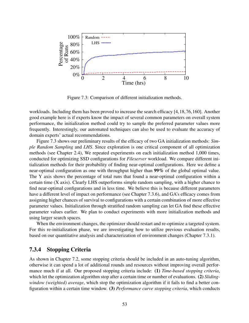
0%

20%

40%

60%

80%

100%

0 2 4 6 8 10

Per

cen

tag

eo

f R

un

s

Time (hrs)

Random

LHS

Figure 7.3: Comparison of different initialization methods.

workloads. Including them has been proved to increase the search efficacy [4,18,76,160]. Anothergood example here is if experts know the impact of several common parameters on overall systemperformance, the initialization method could try to sample the preferred parameter values morefrequently. Interestingly, our automated techniques can also be used to evaluate the accuracy ofdomain experts’ actual recommendations.

Figure 7.3 shows our preliminary results of the efficacy of two GA initialization methods: Sim-ple Random Sampling and LHS. Since exploration is one critical component of all optimizationmethods (see Chapter 2.4), We repeated experiments on each initialization method 1,000 times,conducted for optimizing SSD configurations for Fileserver workload. We compare different ini-tialization methods for their probability of finding near-optimal configurations. Here we define anear-optimal configuration as one with throughput higher than 99% of the global optimal value.The Y axis shows the percentage of total runs that found a near-optimal configuration within acertain time (X axis). Clearly LHS outperforms simple random sampling, with a higher chance tofind near-optimal configurations and in less time. We believe this is because different parametershave a different level of impact on performance (see Chapter 7.3.6), and GA’s efficacy comes fromassigning higher chances of survival to configurations with a certain combination of more effectiveparameter values. Initialization through stratified random sampling can let GA find these effectiveparameter values earlier. We plan to conduct experiments with more initialization methods andusing larger search spaces.

When the environment changes, the optimizer should restart and re-optimize a targeted system.For this re-initialization phase, we are investigating how to utilize previous evaluation results,based on our quantitative analysis and characterization of environment changes (Chapter 7.3.1).

7.3.4 Stopping CriteriaAs shown in Chapter 7.2, some stopping criteria should be included in an auto-tuning algorithm,otherwise it can spend a lot of additional rounds and resources without improving overall perfor-mance much if at all. Our proposed stopping criteria include: (1) Time-based stopping criteria,which let the optimization algorithm stop after a certain time or number of evaluations. (2) Sliding-window (weighted) average, which stop the optimization algorithm if it fails to find a better con-figuration within a certain time window. (3) Performance curve stopping criteria, which conducts

53

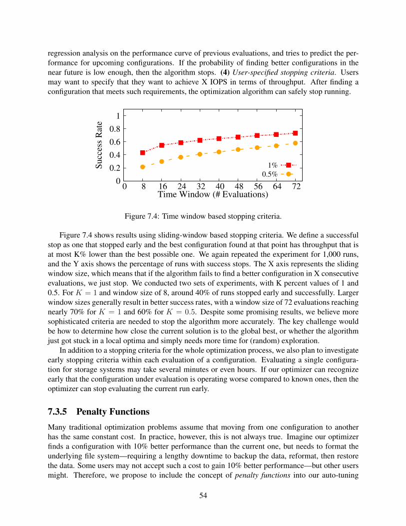
regression analysis on the performance curve of previous evaluations, and tries to predict the per-formance for upcoming configurations. If the probability of finding better configurations in thenear future is low enough, then the algorithm stops. (4) User-specified stopping criteria. Usersmay want to specify that they want to achieve X IOPS in terms of throughput. After finding aconfiguration that meets such requirements, the optimization algorithm can safely stop running.

0

0.2

0.4

0.6

0.8

1

0 8 16 24 32 40 48 56 64 72

Su

ccess

Rate

Time Window (# Evaluations)

1%

0.5%

Figure 7.4: Time window based stopping criteria.

Figure 7.4 shows results using sliding-window based stopping criteria. We define a successfulstop as one that stopped early and the best configuration found at that point has throughput that isat most K% lower than the best possible one. We again repeated the experiment for 1,000 runs,and the Y axis shows the percentage of runs with success stops. The X axis represents the slidingwindow size, which means that if the algorithm fails to find a better configuration in X consecutiveevaluations, we just stop. We conducted two sets of experiments, with K percent values of 1 and0.5. For K = 1 and window size of 8, around 40% of runs stopped early and successfully. Largerwindow sizes generally result in better success rates, with a window size of 72 evaluations reachingnearly 70% for K = 1 and 60% for K = 0.5. Despite some promising results, we believe moresophisticated criteria are needed to stop the algorithm more accurately. The key challenge wouldbe how to determine how close the current solution is to the global best, or whether the algorithmjust got stuck in a local optima and simply needs more time for (random) exploration.

In addition to a stopping criteria for the whole optimization process, we also plan to investigateearly stopping criteria within each evaluation of a configuration. Evaluating a single configura-tion for storage systems may take several minutes or even hours. If our optimizer can recognizeearly that the configuration under evaluation is operating worse compared to known ones, then theoptimizer can stop evaluating the current run early.

7.3.5 Penalty FunctionsMany traditional optimization problems assume that moving from one configuration to anotherhas the same constant cost. In practice, however, this is not always true. Imagine our optimizerfinds a configuration with 10% better performance than the current one, but needs to format theunderlying file system—requiring a lengthy downtime to backup the data, reformat, then restorethe data. Some users may not accept such a cost to gain 10% better performance—but other usersmight. Therefore, we propose to include the concept of penalty functions into our auto-tuning

54

framework. This penalty roughly correlates to how much downtime the system has to endurewhile moving to a new configuration. We can broadly categorize system parameters into severalpenalty classes from least to most onerous. We expect to need only a small number of categories(shown in Table 7.1), but the exact number and granularity is still being investigated.

Category Penalty Description Examples0 Dynamically changeable vm.dirty ratio (kernel)

1 Restarting app orremounting f/s.

journal option (Ext4),I/O sched. (kernel)

2 Rebooting OSnew kernel image

installed

3 Recreating f/s, requiringdata migration

block size (Ext4), f/stype (kernel)

Table 7.1: Categories of parameter penalties

To identify the penalties associated with each system parameter, administrators have to labelthem and also come up with weights for each category in the beginning. Such labels need onlybe done once for each system parameter, and can then be disseminated publicly. Users, however,would need to assign weights to the various penalty classes in each environment (e.g., more con-servative in production, more aggressive in experimental systems); we are investigating severaldefault weights.

Our optimizer can then take into account the penalties when making decisions. One approachis to include the penalty into the optimization objective function, and thus the objective becomes acomplex cost formula (similar to our economics-based cost functions [97]), rather than one singlesystem metric like I/O throughput.

7.3.6 Machine LearningDespite the issues discussed in Chapter 2.1, we believe that ML can be helpful in our auto-tuningframework. Figure 7.2 highlights with green circles where we feel that ML can be useful asdescribed next.

Initialization As described in §7.3.3, the Optimizer has to re-optimize the system when the envi-ronment changes. One applicable ML area, named Transfer Learning, uses data from prior studiesto guide and accelerate current ones [10, 60, 169]. To guide the optimization process more effec-tively, we are investigating how to transfer evaluation results and workload models (§7.3.1) fromone environment to another.

Stopping criteria In addition to the stopping criteria described in §7.3.4, we will also developand test ML-based stopping criteria. As our optimizer picks configurations to evaluate, over timeit collects more and more useful data, which can be used for incremental model training. Wecan use the data to train ML models to predict the performance of system configurations. If theprobability of getting a better configuration than the current best one is low, the optimizer can stopthe optimization process.

55

Selection ML can help the selection phase in several ways. For example, ML can predict theperformance of the next configuration picked, and thus save time on evaluating unpromising ones.In the beginning, the prediction accuracy would be low due to lack of training data; hence theoptimizer will need to determine a confidence level in the ML model’s accuracy. ML can alsohelp guide the optimizer to pick configurations from unexplored sub-spaces; it can label each con-figuration according to how many in its neighborhood have been explored. Moreover, ML canhelp our auto-tuning framework to identify important parameters and automatically select them.In our past work, we observed that parameters have different importance to the optimization objec-tive [43, 94, 132, 148]. By finding out unrelated or less important parameters and removing themduring the optimization process, we can exponentially reduce the search space [35, 70].

Restarting criteria The ML-aided restarting criteria is related to the Workload Modeler. Ouroptimizer needs to restart when the environment changes enough. We propose to develop an intel-ligent approach with the help of ML techniques, to identify changes in the environment automati-cally.

7.3.7 VisualizerVisual Analytics (VA) techniques include a mix of automated and user-driven actions to improvethe understanding of large-dimensional data sets. The human eye and brain can recognize patternsthat computers are yet unable to. By visualizing N-dimensional spaces into 2D/3D, we will dis-cover patterns that will help us (domain experts) develop more effective optimization techniques.VA will help us discover complex correlations among search parameters (i.e., dimensions, at-tributes, features), enabling us to reduce the overall search space size. Our search spaces are solarge because each additional parameter effectively increases the search space exponentially; there-fore, reducing the search space must also be done exponentially. We will integrate feature reductionmethods to reduce the search space: e.g., parameters that have little impact on overall performancecan be removed, and highly correlated parameters can be combined. VA will also help us visualizeand hence evaluate the efficacy of any of our proposed methods and options therein: seeing an n-Dspace in 2D/3D, as its landscape is gradually revealed via more search points; identifying the pathany search technique takes through the space and the path’s efficiency; enabling domain expertsoptionally to provide hints to the search process (e.g., to refocus a search in an unexplored area thedomain expert believes is promising); visualizing the cumulative and current penalty to move to anew configuration; the location and distribution of initially selected configurations; and more.

56

Chapter 8

Proposed and Future Work

In this chapter, we provide a summary of work that we propose to accomplish in this thesis, as wellas future work beyond this thesis.

8.1 Proposed WorkOur proposed work consist of three parts: 1) Experimenting with larger parameter space; 2) De-sign and implement new components for a practical auto-tuning framework; and 3) Design andimplement a workload modeler. We re-colored Figure 7.1 and Figure 7.2 here as Figure 8.1 andFigure 8.2, respectively, to provide a clearer overview of our proposed and future work. Compo-nents are re-colored based on our project timeline. We plan to completely finish work colored bygreen and partially finish work colored by yellow. Components colored with red are left for futurework beyond this thesis.

Experimenting with larger and more complex parameter spaces Our current experimentswere conducted on a 9-parameter space with 6,222 unique configurations. We plan to extend ourexperiments to larger and more complex parameter spaces, which we denote as Storage V3 andStorage V4.

• Storage V3: It will consist of all categories of parameters (as shown in Table 7.1) carefullychosen from several representative local file systems. Unlike the default workloads used inour previous experiments (see Table 4.2), which are assigned with relatively small datasetsize to speed up the whole exhaustive search process, we will apply various workloads withlarger dataset size (at least 2× the RAM size) on Storage V3. We will exhaustively evaluateall configurations in Storage V3. The collected datasets will allow us to design and test ourpractical framework.

• Storage V4: It will be an even larger parameter space, where exhaustive search is impossible.We will use it to test the efficacy of our auto-tuning framework in real-time.

Practical auto-tuning framework We propose to design and implement a practical real-timeauto-tuning framework for storage systems, with new features that are missing from traditionalblack-box optimization techniques. The details are listed as follows:

57

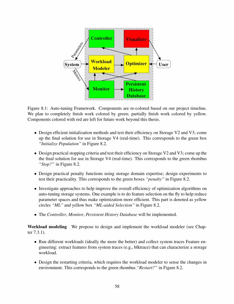
Monitor

Modeler

Workload Optimizer

Visualizer

UserSystem

Para

mete

rs

Metric

s

History

Controller

Database

Persistent

Figure 8.1: Auto-tuning Framework. Components are re-colored based on our project timeline.We plan to completely finish work colored by green; partially finish work colored by yellow.Components colored with red are left for future work beyond this thesis.

• Design efficient initialization methods and test their efficiency on Storage V2 and V3; comeup the final solution for use in Storage V4 (real-time). This corresponds to the green box“Initialize Population” in Figure 8.2.

• Design practical stopping criteria and test their efficiency on Storage V2 and V3; come up thethe final solution for use in Storage V4 (real-time). This corresponds to the green rhombus“Stop?” in Figure 8.2.

• Design practical penalty functions using storage domain expertise; design experiments totest their practicality. This corresponds to the green boxes “penalty” in Figure 8.2.

• Investigate approaches to help improve the overall efficiency of optimization algorithms onauto-tuning storage systems. One example is to do feature selection on the fly to help reduceparameter spaces and thus make optimization more efficient. This part is denoted as yellowcircles “ML” and yellow box “ML-aided Selection” in Figure 8.2.

• The Controller, Monitor, Persistent History Database will be implemented.

Workload modeling We propose to design and implement the workload modeler (see Chap-ter 7.3.1).

• Run different workloads (ideally the more the better) and collect system traces Feature en-gineering: extract features from system traces (e.g., blktrace) that can characterize a storageworkload.

• Design the restarting criteria, which requires the workload modeler to sense the changes inenvironment. This corresponds to the green rhombus “Restart?” in Figure 8.2.

58

Yes

Start

EvaluateFitness

New

Population

Yes

No

No

Mutation CrossoverStop?

ElitismML−aided Penalty

ML

ML

Restart?

Penalty

InitializePopulation

Selection

Selection

ML

Figure 8.2: Work flow for an enhanced Optimizer (GA). Components are re-colored based on ourproject timeline. We plan to completely finish work colored by green; partially finish work coloredby yellow. Components colored with red are left for future work beyond this thesis.

• If time permits, quantify the similarities between workloads and come up with solutionsto transfer and reuse previous evaluation results. This is why the “Workload Modeler” ismarked as yellow (partially finished by thesis defense) in Figure 8.2.

8.2 Future WorkThis work can be extended further beyond the scope of the thesis. We see at least the followinginteresting and promising directions.

• Use visual analytics to help understand our parameter spaces and datasets. It might also beuseful in showing intermediate status of optimization algorithms to storage domain experts,who then can make difficult decisions for the auto-tuning framework. This corresponds tothe red box “Visualizer” in Figure 8.1.

• Find the minimum set of system metrics that can characterize a storage workload. This is notonly useful for our auto-tuning framework, but could have broader impacts on understandingand optimizing performance for all storage systems. This will be part of the “WorkloadModeler” in Figure 8.1.

• Design hybrid algorithms that combine traditional optimization algorithms and ML tech-niques. This is part of the “Optimizer” in Figure 8.1.

59

Chapter 9

Conclusions

Optimizing storage systems can provide significant benefits especially in improving I/O perfor-mance. Alas, storage systems are getting more complex, contain many parameters and an im-mense number of possible configurations; manual tuning is therefore impractical. Worse, many ofthose parameters are non-linear or non-numeric; traditional linear-regression-based optimizationtechniques do not work well for such problems. Therefore, in this work, we propose to auto-tunestorage system configurations in real-time.

We first performed a comparative study on various black-box optimization algorithms. (1) Weevaluated five popular but different auto-tuning techniques, varied some of their hyper-parameters,and applied them to storage and file systems. (2) We show that the speed at which the techniquescan find optimal or near-optimal configurations (in terms of throughput) depends on the hardware,software, and workload; this means that no single technique can “rule them all.” (3) We explainwhy some techniques appear to work better than others.

In our auto-tuning experiments, we observed that repeated experiments in well-controlled,identical environments could produce results with high variations. Therefore, we then providedthe first systematic study on performance variation in benchmarking a modern storage system. Weshowed that variation is common in storage systems, although its magnitude depends heavily onspecific configurations and workloads. Our analysis revealed that block allocation is a major causeof performance variation in Ext4-HDD configurations. From the temporal view, the magnitude ofthroughput variation also depends on the window size and changes over time. The latency distri-bution for the same operation type could also vary even over repeated runs of the same experiment.We quantified the correlation between performance and latency variations using a novel approach.

Our preliminary results show that applying black-box optimization techniques to auto-tunestorage system configurations are feasible and promising, but also indicate several limitations.Therefore, we propose to design a more intelligent and practical framework for real-time auto-tuning storage systems, with several new components: a workload modeler to characterize a run-ning workload dynamically; stopping criteria to save resources; restarting criteria in response toenvironment changes; and effective initialization and ML-aided selection methods, including di-mensionality reduction, to speed up the auto-tuning process. We conducted simple experiments todemonstrate that our framework is the right direction for auto-tuning storage system in real-time.

Another big contribution of our project is that we are collecting a lot of data on evaluatingdifferent storage configurations on various workloads. For more than two years, we have collecteda large data-set of over 450,000 data points. In our proposed work, we will conduct experiments

60

on even more complex parameter space in the near future. All our results will be stored in acarefully designed database. We plan to release our datasets in the future, to facilitate research onunderstanding and optimizing storage performance.

Finally, it is our thesis that real-time auto-tuning storage systems is important, promising, andfeasible with a carefully designed framework to include missing yet critical features. We hope ourauto-tuning framework can improve systems’ performance efficiency, and save energy and humanresources in the long term.

61

Bibliography

[1] Emile Aarts and Jan Korst. Simulated annealing and Boltzmann machines. New York, NY;John Wiley and Sons Inc., 1988.

[2] Abutalib Aghayev, Mansour Shafaei, and Peter Desnoyers. Skylight—a window on shingleddisk operation. Trans. Storage, 11(4):16:1–16:28, October 2015.

[3] Abutalib Aghayev, Theodore Ts’o, Garth Gibson, and Peter Desnoyers. Evolving ext4 forshingled disks. In Proceedings of the 15th USENIX Conference on File and Storage Tech-nologies (FAST), pages 105–120, Santa Clara, CA, February/March 2017. USENIX Asso-ciation.

[4] Ravindra K Ahuja and James B Orlin. Developing fitter genetic algorithms. INFORMSJournal on Computing, 9(3):251–253, 1997.

[5] Omid Alipourfard, Hongqiang Harry Liu, Jianshu Chen, Shivaram Venkataraman, MinlanYu, and Ming Zhang. Cherrypick: Adaptively unearthing the best cloud configurationsfor big data analytics. In 14th USENIX Symposium on Networked Systems Design andImplementation (NSDI 17), pages 469–482. USENIX Association, 2017.

[6] Guillermo A. Alvarez, Elizabeth Borowsky, Susie Go, Theodore H. Romer, Ralph Becker-Szendy, Richard Golding, Arif Merchant, Mirjana Spasojevic, Alistair Veitch, and JohnWilkes. Minerva: An automated resource provisioning tool for large-scale storage systems.ACM Trans. Comput. Syst., 19(4):483–518, November 2001.

[7] Terry Anderson. The theory and practice of online learning. Athabasca University Press,2008.

[8] R. H. Arpaci-Dusseau, E. Anderson, N. T., D. E. Culler, J. M. Hellerstein, D. Patterson,and K. Yelick. Cluster I/O with river: making the fast case common. In Workshop onInput/Output in Parallel and Distributed Systems, pages 10–22, Atlanta, GA, May 1999.

[9] Remzi H. Arpaci-Dusseau and Andrea C. Arpaci-Dusseau. Operating Systems: Three EasyPieces. Arpaci-Dusseau Books, 0.91 edition, May 2015.

[10] Remi Bardenet, Matyas Brendel, Balazs Kegl, and Michele Sebag. Collaborative hyperpa-rameter tuning. In Proceedings of the 30th International Conference on Machine Learning,volume 28 of Proceedings of Machine Learning Research, pages 199–207. PMLR, 17–19Jun 2013.

62

[11] Babak Behzad, Joey Huchette, Huong Luu, Ruth Aydt, Quincey Koziol, Mr Prabhat, SurenByna, Mohamad Chaarawi, and Yushu Yao. Auto-tuning of parallel io parameters for hdf5applications. In Proceedings of the 2012 SC Companion: High Performance Computing,Networking Storage and Analysis, SCC ’12, pages 1430–, Washington, DC, USA, 2012.IEEE Computer Society.

[12] Babak Behzad, Huong Vu Thanh Luu, Joseph Huchette, Surendra Byna, Prabhat, Ruth Aydt,Quincey Koziol, and Marc Snir. Taming parallel i/o complexity with auto-tuning. In Pro-ceedings of the International Conference on High Performance Computing, Networking,Storage and Analysis, SC ’13, pages 68:1–68:12, New York, NY, USA, 2013. ACM.

[13] Irwan Bello, Hieu Pham, Quoc V Le, Mohammad Norouzi, and Samy Bengio. Neuralcombinatorial optimization with reinforcement learning. arXiv preprint arXiv:1611.09940,2016.

[14] James Bergstra and Yoshua Bengio. Random search for hyper-parameter optimization. Jour-nal of Machine Learning Research, 13(Feb):281–305, 2012.

[15] James S. Bergstra, Remi Bardenet, Yoshua Bengio, and Balazs Kegl. Algorithms for hyper-parameter optimization. In Advances in Neural Information Processing Systems 24, pages2546–2554, 2011.

[16] MC Bhuvaneswari. Application of Evolutionary Algorithms for Multi-objective Optimiza-tion in VLSI and Embedded Systems. Springer, 2015.

[17] D. Boutcher and A. Chandra. Does virtualization make disk scheduling passe? In Proceed-ings of the 1st USENIX Workshop on Hot Topics in Storage and File Systems (HotStorage’09), October 2009.

[18] Mark F Bramlette. Initialization, mutation and selection methods in genetic algorithms forfunction optimization. In ICGA, pages 100–107, 1991.

[19] Eric Brochu, Vlad M Cora, and Nando De Freitas. A tutorial on bayesian optimizationof expensive cost functions, with application to active user modeling and hierarchical rein-forcement learning. arXiv preprint arXiv:1012.2599, 2010.

[20] BTRFS. http://btrfs.wiki.kernel.org/.

[21] Axel Busch, Qais Noorshams, Samuel Kounev, Anne Koziolek, Ralf Reussner, and ErichAmrehn. Automated workload characterization for i/o performance analysis in virtualizedenvironments. In Proceedings of the 6th ACM/SPEC International Conference on Perfor-mance Engineering, pages 265–276. ACM, 2015.

[22] M. Cao, T. Y. Ts’o, B. Pulavarty, S. Bhattacharya, A. Dilger, and A. Tomas. State of the art:Where we are with the Ext3 filesystem. In Proceedings of the Linux Symposium, Ottawa,ON, Canada, July 2005.

[23] Zhen Cao. Parametric optimization of storage systems. Technical Report FSL-16-01, Com-puter Science Department, Stony Brook University, January 2016.

63

[24] Zhen Cao, Vasily Tarasov, Hari Raman, Dean Hildebrand, and Erez Zadok. On the perfor-mance variation in modern storage stacks. In Proceedings of the 15th USENIX Conferenceon File and Storage Technologies (FAST), pages 329–343, Santa Clara, CA, February/March2017. USENIX Association.

[25] R. Card, T. Ts’o, and S. Tweedie. Design and implementation of the second extendedfilesystem. In Proceedings to the First Dutch International Symposium on Linux, Seattle,WA, December 1994.

[26] George Casella and Roger L Berger. Statistical Inference, volume 2. Duxbury Pacific Grove,CA, 2002.

[27] Vladimır Cerny. Thermodynamical approach to the traveling salesman problem: An effi-cient simulation algorithm. Journal of optimization theory and applications, 45(1):41–51,1985.

[28] Kevin K. Chang, Abhijith Kashyap, Hasan Hassan, Saugata Ghose, Kevin Hsieh, DonghyukLee, Tianshi Li, Gennady Pekhimenko, Samira Khan, and Onur Mutlu. Understanding la-tency variation in modern DRAM chips: Experimental characterization, analysis, and op-timization. In Proceedings of the 2016 ACM SIGMETRICS International Conference onMeasurement and Modeling of Computer Science, SIGMETRICS’16, pages 323–336, NewYork, NY, USA, 2016. ACM.

[29] Min Chen, Shiwen Mao, and Yunhao Liu. Big data: A survey. Mobile Networks andApplications, 19(2):171–209, 2014.

[30] Y. Chen, M. Winslett, Y. Cho, and S. Kuo. Automatic parallel i/o performance optimizationusing genetic algorithms. In Proceedings of the 7th IEEE International Symposium on HighPerformance Distributed Computing, HPDC ’98, pages 155–, Washington, DC, USA, 1998.IEEE Computer Society.

[31] Maurice Clerc. Particle swarm optimization, volume 93. John Wiley & Sons, 2010.

[32] Yvonne Coady, Russ Cox, John DeTreville, Peter Druschel, Joseph Hellerstein, AndrewHume, Kimberly Keeton, Thu Nguyen, Christopher Small, Lex Stein, and Andrew Warfield.Falling off the cliff: When systems go nonlinear. In Proceedings of the 10th Conference onHot Topics in Operating Systems - Volume 10, HOTOS’05, 2005.

[33] James Cohoon, John Kairo, and Jens Lienig. Evolutionary algorithms for the physical designof vlsi circuits. In Advances in evolutionary computing, pages 683–711. Springer, 2003.

[34] Valentin Dalibard, Michael Schaarschmidt, and Eiko Yoneki. Boat: Building auto-tunerswith structured bayesian optimization. In Proceedings of the 26th International Conferenceon World Wide Web, WWW ’17, pages 479–488. International World Wide Web Confer-ences Steering Committee, 2017.

[35] Kenneth Alan De Jong. Analysis of the behavior of a class of genetic adaptive systems. PhDthesis, University of Michigan, Ann Arbor, Ann Arbor, MI, USA, 1975.

64

[36] Pablo de Oliveira Castro, Yuriy Kashnikov, Chadi Akel, Mihail Popov, and WilliamJalby. Fine-grained benchmark subsetting for system selection. In Proceedings of An-nual IEEE/ACM International Symposium on Code Generation and Optimization, page 132.ACM, 2014.

[37] Jeffrey Dean and Luiz Andre Barroso. The tail at scale. Commun. ACM, 56(2):74–80,February 2013.

[38] Peter Desnoyers. Empirical evaluation of nand flash memory performance. In HotStorage’09: Proceedings of the 1st Workshop on Hot Topics in Storage. ACM, 2009.

[39] Y. Diao, J. L. Hellerstein, A. J. Storm, M. Surendra, S. Lightstone, S. Parekh, and C. Garcia-Arellano. Using MIMO linear control for load balancing in computing systems. In 2004American Control Conferences, 2004.

[40] Marco Dorigo and Mauro Birattari. Ant colony optimization. In Encyclopedia of machinelearning, pages 36–39. Springer, 2010.

[41] Marco Dorigo, Mauro Birattari, and Thomas Stutzle. Ant colony optimization. Computa-tional Intelligence Magazine, IEEE, 1(4):28–39, 2006.

[42] Fred Douglis, Deepti Bhardwaj, Hangwei Qian, and Philip Shilane. Content-aware loadbalancing for distributed backup. In LISA, 2011.

[43] E. Zadok and A. Arora and Z. Cao and A. Chaganti and A. Chaudhary and S. Mandal. Para-metric optimization of storage systems. In HotStorage ’15: Proceedings of the 7th USENIXWorkshop on Hot Topics in Storage, Santa Clara, CA, July 2015. USENIX, USENIX.

[44] Katharina Eggensperger, Matthias Feurer, Frank Hutter, James Bergstra, Jasper Snoek,Holger Hoos, and Kevin Leyton-Brown. Towards an empirical foundation for assessingbayesian optimization of hyperparameters. In NIPS workshop on Bayesian Optimization inTheory and Practice, volume 10, 2013.

[45] A.E. Eiben and C.A. Schippers. On evolutionary exploration and exploitation. Fundam.Inf., 35(1-4):35–50, January 1998.

[46] Nosayba El-Sayed, Ioan A. Stefanovici, George Amvrosiadis, Andy A. Hwang, and BiancaSchroeder. Temperature management in data centers: Why some (might) like it hot. In Pro-ceedings of the 12th ACM SIGMETRICS/PERFORMANCE Joint International Conferenceon Measurement and Modeling of Computer Systems, SIGMETRICS’12, pages 163–174,New York, NY, USA, 2012. ACM.

[47] Ext4. http://ext4.wiki.kernel.org/.

[48] Ext4 documentation. https://www.kernel.org/doc/Documentation/filesystems/ext4.txt.

[49] Linux/fs/ext4/ialloc.c. http://lxr.free-electrons.com/source/fs/ext4/ialloc.c.

65

[50] Filebench, 2016. https://github.com/filebench/filebench/wiki.

[51] Terry L Friesz, Hsun-Jung Cho, Nihal J Mehta, Roger L Tobin, and G Anandalingam. Asimulated annealing approach to the network design problem with variational inequalityconstraints. Transportation Science, 26(1):18–26, 1992.

[52] RA Gallego, AB Alves, A Monticelli, and R Romero. Parallel simulated annealing appliedto long term transmission network expansion planning. Power Systems, IEEE Transactionson, 12(1):181–188, 1997.

[53] Shravan Gaonkar, Kimberly Keeton, Arif Merchant, and William H. Sanders. Designingdependable storage solutions for shared application environments. IEEE Trans. DependableSecur. Comput., 7(4):366–380, October 2010.

[54] Michel Gendreau and Jean-Yves Potvin. Handbook of metaheuristics, volume 2. Springer,2010.

[55] S. Ghemawat, H. Gobioff, and S. T. Leung. The Google file system. In Proceedings of the19th ACM Symposium on Operating Systems Principles (SOSP ’03), pages 29–43, BoltonLanding, NY, October 2003. ACM SIGOPS.

[56] F. Glover. Tabu Search – Part II. ORSA Journal on Computing, 2:4–32, 1990.

[57] Fred Glover. Tabu search: A tutorial. Interfaces, 20(4):74–94, 1990.

[58] Fred Glover and Manuel Laguna. Tabu Search. Springer, 2013.

[59] David E Goldberg and Robert Lingle. Alleles, loci, and the traveling salesman problem. InProceedings of the first international conference on genetic algorithms and their applica-tions, pages 154–159. Lawrence Erlbaum Associates, Publishers, 1985.

[60] Daniel Golovin, Benjamin Solnik, Subhodeep Moitra, Greg Kochanski, John Karro, andD. Sculley. Google vizier: A service for black-box optimization. In Proceedings of the 23rdACM SIGKDD International Conference on Knowledge Discovery and Data Mining, KDD’17, pages 1487–1495. ACM, 2017.

[61] Ian Goodfellow, Yoshua Bengio, and Aaron Courville. Deep Learning. MIT Press, 2016.http://www.deeplearningbook.org.

[62] John Grefenstette, Rajeev Gopal, Brian Rosmaita, and Dirk Van Gucht. Genetic algorithmsfor the traveling salesman problem. In Proceedings of the first International Conference onGenetic Algorithms and their Applications, pages 160–168. Lawrence Erlbaum, New Jersey(160-168), 1985.

[63] Lov K Grover. A new simulated annealing algorithm for standard cell placement. In Pro-ceedings of the International Conference on Computer-Aided Design, pages 378–380, 1986.

66

[64] Mingzhe Hao, Gokul Soundararajan, Deepak Kenchammana-Hosekote, Andrew A Chien,and Haryadi S Gunawi. The tail at store: a revelation from millions of hours of disk andssd deployments. In 14th USENIX Conference on File and Storage Technologies (FAST 16),pages 263–276, 2016.

[65] Md E. Haque, Yong hun Eom, Yuxiong He, Sameh Elnikety, Ricardo Bianchini, andKathryn S. McKinley. Few-to-many: Incremental parallelism for reducing tail latency ininteractive services. In Proceedings of the Twentieth International Conference on Archi-tectural Support for Programming Languages and Operating Systems, ASPLOS’15, pages161–175, New York, NY, USA, 2015. ACM.

[66] Georges R Harik and Fernando G Lobo. A parameter-less genetic algorithm. In GECCO,volume 99, pages 258–267, 1999.

[67] Jun He, Duy Nguyen, Andrea C. Arpaci-Dusseau, and Remzi H. Arpaci-Dusseau. Reducingfile system tail latencies with Chopper. In Proceedings of the 13th USENIX Conferenceon File and Storage Technologies, FAST’15, pages 119–133, Berkeley, CA, USA, 2015.USENIX Association.

[68] Weiping He and David H.C. Du. Smart: An approach to shingled magnetic recording trans-lation. In Proceedings of the 15th USENIX Conference on File and Storage Technologies(FAST), pages 121–134, Santa Clara, CA, February/March 2017. USENIX Association.

[69] J. L. Hellerstein, Y. Diao, S. Parekh, and D. M. Tibury. Feedback Control of ComputingSystems. Wiley-IEEE Press, 2004.

[70] J. H. Holland. Adaptation in natural and artificial systems: An introductory analysis withapplications to biology, control, and artificial intelligence. U. Michigan Press, 1975.

[71] Ronald L Iman, Jon C Helton, James E Campbell, et al. An approach to sensitivity analysisof computer models, part 1. introduction, input variable selection and preliminary variableassessment. Journal of quality technology, 13(3):174–183, 1981.

[72] Myeongjae Jeon, Saehoon Kim, Seung-won Hwang, Yuxiong He, Sameh Elnikety, Alan L.Cox, and Scott Rixner. Predictive parallelization: Taming tail latencies in web search. InProceedings of the 37th International ACM SIGIR Conference on Research & Developmentin Information Retrieval, SIGIR’14, pages 253–262, New York, NY, USA, 2014. ACM.

[73] Young-Jae Jeon, Jae-Chul Kim, Jin-O Kim, Joong-Rin Shin, and Kwang Y Lee. An effi-cient simulated annealing algorithm for network reconfiguration in large-scale distributionsystems. Power Delivery, IEEE Transactions on, 17(4):1070–1078, 2002.

[74] N. Joukov, A. Traeger, R. Iyer, C. P. Wright, and E. Zadok. Operating system profiling vialatency analysis. In Proceedings of the 7th Symposium on Operating Systems Design andImplementation (OSDI 2006), pages 89–102, Seattle, WA, November 2006. ACM SIGOPS.

[75] Karthik Kambatla, Giorgos Kollias, Vipin Kumar, and Ananth Grama. Trends in big dataanalytics. Journal of Parallel and Distributed Computing, 74(7):2561–2573, 2014. SpecialIssue on Perspectives on Parallel and Distributed Processing.

67

[76] A Kapsalis, Vic J Rayward-Smith, and George D Smith. Solving the graphical steiner treeproblem using genetic algorithms. Journal of the Operational Research Society, pages 397–406, 1993.

[77] M. Karlsson, C. Karamanolis, and X. Zhu. Triage: Performance differentiation for storagesystems using adaptive control. ACM Trans. Storage, 1(4), 2005.

[78] Kimberly Keeton, Dirk Beyer, Ernesto Brau, Arif Merchant, Cipriano Santos, and AlexZhang. On the road to recovery: Restoring data after disasters. In Proceedings of the1st ACM SIGOPS/EuroSys European Conference on Computer Systems 2006, EuroSys’06,pages 235–248, New York, NY, USA, 2006. ACM.

[79] James Kennedy. Particle swarm optimization. In Encyclopedia of Machine Learning, pages760–766. Springer, 2010.

[80] James Kennedy and Russell C. Eberhart. Particle swarm optimization. In Proceedings ofthe IEEE International Conference on Neural Networks, pages 1942–1948, 1995.

[81] H. Kim, S. Seshadri, C. L. Dickey, and L. Chiu. Evaluating phase change memory forenterprise storage systems: A study of caching and tiering approaches. In Proceedings ofthe 12th USENIX Conference on File and Storage Technologies, pages 33–45, Berkeley,CA, 2014. USENIX.

[82] S. Kirkpatrick, C D. Gelatt, M. P Vecchi, et al. Optimization by simulated annealing. sci-ence, 220(4598):671–680, 1983.

[83] Ryusuke Konishi, Yoshiji Amagai, Koji Sato, Hisashi Hifumi, Seiji Kihara, and SatoshiMoriai. The linux implementation of a log-structured file system. ACM SIGOPS OperatingSystems Review, 40(3):102–107, 2006.

[84] Natalio Krasnogor and Jim Smith. A tutorial for competent memetic algorithms: model,taxonomy, and design issues. Evolutionary Computation, IEEE Transactions on, 9(5):474–488, 2005.

[85] Sajib Kundu, Raju Rangaswami, Ajay Gulati, Ming Zhao, and Kaushik Dutta. Modelingvirtualized applications using machine learning techniques. In Proceedings of the 8th ACMSIGPLAN/SIGOPS Conference on Virtual Execution Environments, VEE ’12, pages 3–14.ACM, 2012.

[86] Pedro Larranaga, Cindy M. H. Kuijpers, Roberto H. Murga, Inaki Inza, and Sejla Dizdare-vic. Genetic algorithms for the travelling salesman problem: A review of representationsand operators. Artificial Intelligence Review, 13(2):129–170, 1999.

[87] Changman Lee, Dongho Sim, Jooyoung Hwang, and Sangyeun Cho. F2fs: A new file sys-tem for flash storage. In Proceedings of the 13th USENIX Conference on File and StorageTechnologies (FAST), pages 273–286, Santa Clara, CA, February 2015. USENIX Associa-tion.

68

[88] Ernest Bruce Lee and Lawrence Markus. Foundations of optimal control theory. Technicalreport, DTIC Document, 1967.

[89] H. D. Lee, Y. J. Nam, K. J. Jung, S. G. Jung, and C. Park. Regulating I/O performanceof shared storage with a control theoretical approach. In NASA/IEEE Conference on MassStorage Systems and Technologies (MSST). IEEE Society Press, 2004.

[90] Cheng Li, Philip Shilane, Fred Douglis, Darren Sawyer, and Hyong Shim. As-sert(!defined(sequential i/o)). In 6th USENIX Workshop on Hot Topics in Storage and FileSystems (HotStorage 14), Philadelphia, PA, 2014. USENIX Association.

[91] Jialin Li, Naveen Kr. Sharma, Dan R. K. Ports, and Steven D. Gribble. Tales of the tail:Hardware, os, and application-level sources of tail latency. In Proceedings of the ACMSymposium on Cloud Computing, SoCC’14, pages 9:1–9:14, New York, NY, USA, 2014.ACM.

[92] Yin Li, Hao Wang, Xuebin Zhang, Ning Zheng, Shafa Dahandeh, and Tong Zhang. Fa-cilitating magnetic recording technology scaling for data center hard disk drives throughfilesystem-level transparent local erasure coding. In Proceedings of the 15th USENIX Con-ference on File and Storage Technologies (FAST), pages 135–148, Santa Clara, CA, Febru-ary/March 2017. USENIX Association.

[93] Yuxi Li. Deep reinforcement learning: An overview. arXiv preprint arXiv:1701.07274,2017.

[94] Z. Li, M. Chen, A. Mukker, and E. Zadok. On the trade-offs among performance, energy,and endurance in a versatile hybrid drive. ACM Transactions on Storage (TOS), 11(3), July2015.

[95] Z. Li, K. M. Greenan, A. W. Leung, and E. Zadok. Power consumption in enterprise-scale backup storage systems. In Proceedings of the Tenth USENIX Conference on File andStorage Technologies (FAST ’12), San Jose, CA, February 2012. USENIX Association.

[96] Z. Li, R. Grosu, K. Muppalla, S. A. Smolka, S. D. Stoller, and E. Zadok. Model discoveryfor energy-aware computing systems: An experimental evaluation. In Proceedings of the 1stWorkshop on Energy Consumption and Reliability of Storage Systems (ERSS’11), Orlando,FL, July 2011.

[97] Z. Li, A. Mukker, and E. Zadok. On the importance of evaluating storage systems’ $costs.In Proceedings of the 6th USENIX Conference on Hot Topics in Storage and File Systems,HotStorage’14, 2014.

[98] Chieh-Jan Mike Liang, Jie Liu, Liqian Luo, Andreas Terzis, and Feng Zhao. RACNet:A high-fidelity data center sensing network. In Proceedings of the 7th ACM Conferenceon Embedded Networked Sensor Systems, SenSys’09, pages 15–28, New York, NY, USA,2009. ACM.

69

[99] Jens Lienig and James P Cohoon. Genetic algorithms applied to the physical design ofvlsi circuits: A survey. In Parallel Problem Solving from NaturePPSN IV, pages 839–848.Springer, 1996.

[100] Fernando G Lobo and David E Goldberg. The parameter-less genetic algorithm in practice.Information Sciences, 167(1):217–232, 2004.

[101] Christoffer Loffler, Christopher Mutschler, and Michael Philippsen. Evolutionary algo-rithms that use runtime migration of detector processes to reduce latency in event-basedsystems. In Adaptive Hardware and Systems (AHS), 2013 NASA/ESA Conference on, pages31–38. IEEE, 2013.

[102] W. J. Conover M. D. McKay, R. J. Beckman. A comparison of three methods for selectingvalues of input variables in the analysis of output from a computer code. Technometrics,21(2):239–245, 1979.

[103] Pradipta De Vijay Mann and Umang Mittaly. Handling OS jitter on multicore multithreadedsystems. In Parallel & Distributed Processing Symposium (IPDPS), 2009 IEEE Interna-tional, IPDPS’09, pages 1–12. IEEE, 2009.

[104] Olivier Martin, Steve W Otto, and Edward W Felten. Large-step markov chains for the tspincorporating local search heuristics. Operations Research Letters, 11(4):219–224, 1992.

[105] Pinaki Mazumder and Elizabeth M. Rudnick, editors. Genetic Algorithms for VLSI Design,Layout &Amp; Test Automation. Prentice Hall PTR, Upper Saddle River, NJ, USA, 1999.

[106] M. K. McKusick, W. N. Joy, S. J. Leffler, and R. S. Fabry. A fast file system for UNIX.ACM Transactions on Computer Systems, 2(3):181–197, August 1984.

[107] Peter Merz. Memetic algorithms for combinatorial optimization problems: Fitness land-scapes and effective search strategies, 2001.

[108] Justin Meza, Qiang Wu, Sanjev Kumar, and Onur Mutlu. A large-scale study of flash mem-ory failures in the field. In Proceedings of the 2015 ACM International Conference onMeasurement and Modeling of Computer Systems (SIGMETRICS 2015), pages 177–190,Portland, OR, June 2015. ACM.

[109] Sun Microsystems. Lustre file system: High-performance storage architec-ture and scalable cluster file system white paper. www.sun.com/servers/hpc/docs/lustrefilesystem_wp.pdun.com/servers/hpc/docs/lustrefilesystem_wp.pdf, December 2007.

[110] Volodymyr Mnih, Koray Kavukcuoglu, David Silver, Alex Graves, Ioannis Antonoglou,Daan Wierstra, and Martin Riedmiller. Playing atari with deep reinforcement learning.arXiv preprint arXiv:1312.5602, 2013.

[111] Volodymyr Mnih, Koray Kavukcuoglu, David Silver, Andrei A Rusu, Joel Veness, Marc GBellemare, Alex Graves, Martin Riedmiller, Andreas K Fidjeland, Georg Ostrovski, et al.Human-level control through deep reinforcement learning. Nature, 518(7540):529–533,2015.

70

[112] Alessandro Morari, Roberto Gioiosa, Robert W Wisniewski, Francisco J Cazorla, and Ma-teo Valero. A quantitative analysis of OS noise. In Parallel & Distributed ProcessingSymposium (IPDPS), 2011 IEEE International, IPDPS’11, pages 852–863. IEEE, 2011.

[113] Heinz Muhlenbein. Evolution in time and space-the parallel genetic algorithm. In Founda-tions of genetic algorithms. Citeseer, 1991.

[114] Kevin P Murphy. Machine learning: a probabilistic perspective. MIT press, 2012.

[115] Iyswarya Narayanan, Di Wang, Myeongjae Jeon, Bikash Sharma, Laura Caulfield, AnandSivasubramaniam, Ben Cutler, Jie Liu, Badriddine Khessib, and Kushagra Vaid. Ssd fail-ures in datacenters: What? when? and why? In Proceedings of the Second ACM IsraeliExperimental Systems Conference (SYSTOR ’16), pages 7:1–7:11, Haifa, Israel, May 2016.ACM.

[116] E. B. Nightingale, K. Veeraraghavan, P. M. Chen, and J. Flinn. Rethink the sync. In Pro-ceedings of the 7th Symposium on Operating Systems Design and Implementation (OSDI2006), pages 1–14, Seattle, WA, November 2006. ACM SIGOPS.

[117] OpenStack Swift. http://docs.openstack.org/developer/swift/.

[118] Christian S. Perone. Pyevolve: A python open-source framework for genetic algorithms.SIGEVOlution, 4(1):12–20, November 2009.

[119] Esteban Real, Sherry Moore, Andrew Selle, Saurabh Saxena, Yutaka Leon Suematsu,Quoc Le, and Alex Kurakin. Large-scale evolution of image classifiers. arXiv preprintarXiv:1703.01041, 2017.

[120] Jackie Rees and Gary J Koehler. An investigation of ga performance results for differentcardinality alphabets. In Evolutionary Algorithms, pages 191–206. Springer, 1999.

[121] H. Reiser. ReiserFS v.3 whitepaper. http://web.archive.org/web/20031015041320/http://namesys.com/.

[122] Bernd Reisleben and Peter Merz. A genetic local search algorithm for solving symmetricand asymmetric traveling salesman problems. In Evolutionary Computation, 1996., Pro-ceedings of IEEE International Conference on, pages 616–621. IEEE, 1996.

[123] Alma Riska and Erik Riedel. Disk drive level workload characterization. In USENIX AnnualTechnical Conference, volume 2006, pages 97–102, 2006.

[124] Ohad Rodeh, Josef Bacik, and Chris Mason. BTRFS: The Linux B-tree filesystem. Trans.Storage, 9(3):9:1–9:32, August 2013.

[125] Richard P Runyon, Kay A Coleman, and David J Pittenger. Fundamentals of behavioralstatistics . McGraw-Hill, 2000.

71

[126] Anooshiravan Saboori, Guofei Jiang, and Haifeng Chen. Autotuning configurations in dis-tributed systems for performance improvements using evolutionary strategies. In Proceed-ings of the 2008 The 28th International Conference on Distributed Computing Systems,ICDCS ’08, pages 769–776, Washington, DC, USA, 2008. IEEE Computer Society.

[127] Sadiq M Sait, Mahmood R Minhas, Junhaid Khan, et al. Performance and low powerdriven vlsi standard cell placement using tabu search. In Evolutionary Computation, 2002.CEC’02. Proceedings of the 2002 Congress on, volume 1, pages 372–377. IEEE, 2002.

[128] Ricardo Santana, Raju Rangaswami, Vasily Tarasov, and Dean Hildebrand. A fast andslippery slope for file systems. In Proceedings of the 3rd Workshop on Interactions ofNVM/FLASH with Operating Systems and Workloads, INFLOW ’15, pages 5:1–5:8, NewYork, NY, USA, 2015. ACM.

[129] F. Schmuck and R. Haskin. GPFS: A shared-disk file system for large computing clusters.In Proceedings of the First USENIX Conference on File and Storage Technologies (FAST’02), pages 231–244, Monterey, CA, January 2002. USENIX Association.

[130] Bianca Schroeder, Raghav Lagisetty, and Arif Merchant. Flash reliability in production:The expected and the unexpected. In Proceedings of the 14th USENIX Conference on Fileand Storage Technologies (FAST), pages 67–80, Santa Clara, CA, February 2016. USENIXAssociation.

[131] Carl Sechen. VLSI placement and global routing using simulated annealing, volume 54.Springer Science & Business Media, 2012.

[132] P. Sehgal, V. Tarasov, and E. Zadok. Evaluating performance and energy in file system serverworkloads. In Proceedings of the USENIX Conference on File and Storage Technologies(FAST), pages 253–266, San Jose, CA, February 2010. USENIX Association.

[133] Bumjoon Seo, Sooyong Kang, Jongmoo Choi, Jaehyuk Cha, Youjip Won, and SungrohYoon. Io workload characterization revisited: A data-mining approach. IEEE Transactionson Computers, 63(12):3026–3038, 2014.

[134] Burr Settles. Active Learning. Morgan & Claypool Publishers, 2012.

[135] SGI. XFS filesystem structure. http://oss.sgi.com/projects/xfs/papers/xfs_filesystem_structure.pdf.

[136] Bobak Shahriari, Kevin Swersky, Ziyu Wang, Ryan P Adams, and Nando de Freitas. Takingthe human out of the loop: A review of bayesian optimization. Proceedings of the IEEE,104(1):148–175, 2016.

[137] Shai Shalev-Shwartz. Online learning and online convex optimization. Foundations andTrends in Machine Learning, 4(2):107–194, 2011.

[138] Kai Shen, Ming Zhong, and Chuanpeng Li. I/o system performance debugging using model-driven anomaly characterization. In Proceedings of the USENIX Conference on File andStorage Technologies (FAST), San Francisco, CA, December 2005. USENIX Association.

72

[139] Scikit-Optimize. https://scikit-optimize.github.io/.

[140] T Starkweather, S Mcdaniel, D Whitley, K Mathias, D Whitley, et al. A comparison ofgenetic sequencing operators. In Proceedings of the fourth International Conference onGenetic Algorithms, 1991.

[141] John D. Strunk, Eno Thereska, Christos Faloutsos, and Gregory R. Ganger. Using utilityto provision storage systems. In Proceedings of the 6th USENIX Conference on File andStorage Technologies, FAST’08, pages 21:1–21:16, Berkeley, CA, USA, 2008. USENIXAssociation.

[142] Lalith Suresh, Marco Canini, Stefan Schmid, and Anja Feldmann. C3: Cutting tail latencyin cloud data stores via adaptive replica selection. In Proceedings of the 12th USENIXConference on Networked Systems Design and Implementation, NSDI’15, pages 513–527,Berkeley, CA, USA, 2015. USENIX Association.

[143] Richard S Sutton and Andrew G Barto. Reinforcement learning: An introduction. MITpress Cambridge, 1998.

[144] A. Sweeney, D. Doucette, W. Hu, C. Anderson, M. Nishimoto, and G. Peck. Scalability inthe XFS file system. In Proceedings of the Annual USENIX Technical Conference, pages1–14, San Diego, CA, January 1996.

[145] sync(8) - Linux manual page. https://linux.die.net/man/8/sync.

[146] V. Tarasov, S. Bhanage, E. Zadok, and M. Seltzer. Benchmarking file system benchmarking:It *is* rocket science. In Proceedings of HotOS XIII:The 13th USENIX Workshop on HotTopics in Operating Systems, Napa, CA, May 2011.

[147] Vasily Tarasov, Zhen Cao, Ming Chen, and Erez Zadok. The dos and don’ts of file systembenchmarking. FreeBSD Journal, January/February, 2016.

[148] Vasily Tarasov, Abhishek Gupta, Kumar Sourav, Sagar Trehan, and Erez Zadok. Terraincognita: On the practicality of user-space file systems. In HotStorage ’15: Proceedings ofthe 7th USENIX Workshop on Hot Topics in Storage, Santa Clara, CA, July 2015. USENIX,USENIX.

[149] Vasily Tarasov, Erez Zadok, and Spencer Shepler. Filebench: A flexible framework for filesystem benchmarking. ;login: The USENIX Magazine, 41(1):6–12, March 2016.

[150] TensorFlow. https://www.tensorflow.org/.

[151] Olivier Thas. Comparing distributions. Springer, 2010.

[152] A. Traeger, I. Deras, and E. Zadok. DARC: Dynamic analysis of root causes of latencydistributions. In Proceedings of the 2008 International Conference on Measurement andModeling of Computer Systems (SIGMETRICS 2008), pages 277–288, Annapolis, MD, June2008. ACM.

73

[153] Stephen Tweedie. Ext3, journaling filesystem. In Ottawa Linux Symposium,July 2000. http://olstrans.sourceforge.net/release/OLS2000-ext3/OLS2000-ext3.html.

[154] Balajee Vamanan, Hamza Bin Sohail, Jahangir Hasan, and T. N. Vijaykumar. TimeTrader:Exploiting latency tail to save datacenter energy for online search. In Proceedings of the 48thInternational Symposium on Microarchitecture, MICRO’48, pages 585–597, New York,NY, USA, 2015. ACM.

[155] Dana Van Aken, Andrew Pavlo, Geoffrey J. Gordon, and Bohan Zhang. Automatic databasemanagement system tuning through large-scale machine learning. In Proceedings of the2017 ACM International Conference on Management of Data, SIGMOD ’17, pages 1009–1024, 2017.

[156] Peter J Van Laarhoven and Emile H Aarts. Simulated annealing: theory and applications,volume 37. Springer Science & Business Media, 1987.

[157] Matej Crepinsek, Shih-Hsi Liu, and Marjan Mernik. Exploration and exploitation in evolu-tionary algorithms: A survey. ACM Comput. Surv., 45(3):35:1–35:33, July 2013.

[158] Mengzhi Wang, Kinman Au, Anastassia Ailamaki, Anthony Brockwell, Christos Faloutsos,and Gregory R. Ganger. Storage device performance prediction with cart models. In TheIEEE Computer Society’s 12th Annual International Symposium on Modeling, Analysis, andSimulation of Computer and Telecommunications Systems. (MASCOTS), pages 588–595,2004.

[159] S. Weil, S. Brandt, E. Miller, D. Long, and C. Maltzahn. Ceph: A scalable, high-performance distributed file system. In Proceedings of the 7th Symposium on OperatingSystems Design and Implementation (OSDI 2006), pages 307–320, Seattle, WA, November2006. ACM SIGOPS.

[160] Darrell Whitley, Keith Mathias, and Patrick Fitzhorn. Delta coding: An iterative searchstrategy for genetic algorithms. In ICGA, volume 91, pages 77–84. Citeseer, 1991.

[161] Latin Hypercube Sampling. https://en.wikipedia.org/wiki/Latin_hypercube_sampling.

[162] DF Wong, Hon Wai Leong, and HW Liu. Simulated annealing for VLSI design, volume 42.Springer Science & Business Media, 2012.

[163] H-S Philip Wong, Simone Raoux, SangBum Kim, Jiale Liang, John P Reifenberg, BipinRajendran, Mehdi Asheghi, and Kenneth E Goodson. Phase change memory. Proceedingsof the IEEE, 98(12):2201–2227, Dec 2010.

[164] Bowei Xi, Zhen Liu, Mukund Raghavachari, Cathy H. Xia, and Li Zhang. A smart hill-climbing algorithm for application server configuration. In Proceedings of the 13th Interna-tional Conference on World Wide Web, WWW ’04, pages 287–296, New York, NY, USA,2004. ACM.

74

[165] Yunjing Xu, Zachary Musgrave, Brian Noble, and Michael Bailey. Bobtail: Avoiding longtails in the cloud. In Proceedings of the 10th USENIX Conference on Networked SystemsDesign and Implementation, NSDI’13, pages 329–342, Berkeley, CA, USA, 2013. USENIXAssociation.

[166] Ji Xue, Feng Yan, A. Riska, and E. Smirni. Proactive management of systems via hybridanalytic techniques. In Cloud and Autonomic Computing (ICCAC), 2015 International Con-ference on, pages 137–148, Sept 2015.

[167] Ji Xue, Feng Yan, Alma Riska, and Evgenia Smirni. Storage workload isolation via tierwarming: How models can help. In 11th International Conference on Autonomic Computing(ICAC 14), pages 1–11, Philadelphia, PA, June 2014. USENIX Association.

[168] Oceane Bel Ethan L. Miller Darrell D. E. Long Yan Li, Kenneth Chang. Capes: Unsuper-vised system performance tuning using neural network-based deep reinforcement learning.In Proceedings of the International Conference for High Performance Computing, Network-ing, Storage and Analysis, SC ’17, 2017.

[169] Dani Yogatama and Gideon Mann. Efficient transfer learning method for automatic hyper-parameter tuning. In Proceedings of the Seventeenth International Conference on ArtificialIntelligence and Statistics, volume 33 of Proceedings of Machine Learning Research, pages1077–1085, Reykjavik, Iceland, 22–25 Apr 2014. PMLR.

[170] Yang Yu, Hong Qian, and Yi-Qi Hu. Derivative-free optimization via classification. InProceedings of the Thirtieth AAAI Conference on Artificial Intelligence, AAAI’16, pages2286–2292. AAAI Press, 2016.

75

A Practical, Real-Time Auto-Tuning Framework for … · Technical Report FSL-18-01 April 2018....

Documents

Transcript of A Practical, Real-Time Auto-Tuning Framework for … · Technical Report FSL-18-01 April 2018....