Practical Algorithms for Computing STV and OtherMulti-Round Voting Rules

Chunheng JiangRensselaer Polytechnic Inst.Dept. of Computer Science

jiangc4@rpi.edu

Sujoy SikdarRensselaer Polytechnic Inst.Dept. of Computer Science

sikdas@rpi.edu

Hejun WangRensselaer Polytechnic Inst.Dept. of Computer Science

wangj38@rpi.eduLirong Xia

Rensselaer Polytechnic Inst.Dept. of Computer Science

xial@cs.rpi.edu

Zhibing ZhaoRensselaer Polytechnic Inst.Dept. of Computer Science

zhaoz6@rpi.edu

ABSTRACTSTV is one of the most commonly-used voting rules for groupdecision-making, especially for political elections. However,the literature is vague about which tie-breaking mechanismshould be used to eliminate alternatives. We propose thefirst algorithms for computing co-winners under STV, eachof which corresponds to the winner under some tie-breakingmechanism. This problem is known as parallel-universes-tiebreaking (PUT)-STV, which is known to be NP-completeto compute [9]. We conduct experiments on synthetic dataand Preflib data, and show that standard search algorithmswork much better than ILP. We also explore improvementsto the search algorithm with various features including prun-ing, reduction, caching and sampling.

1. INTRODUCTIONVoting is one of the most practical and popular ways for

group decision-making, and is one of the major topics un-der social choice theory. In the past decades there has beena growing literature of computational social choice, whichstudies computational aspects of social choice problems andvoting rules [4]. More recently, computational social choice,in conjunction with algorithmic game theory, has been rec-ognized as one of the eleven “fundamental methods and ap-plication areas” of AI, according to The One Hundred YearStudy on Artificial Intelligence [14].

One of the earliest and the most fundamental problems incomputational social choice is the computation of winners ofwell-studied voting rules. In fact, the widely-regarded firstpaper in computational social choice, published by Bartholdiet al. in 1989 [3], proved that Dodgson’s rule and the Kemenyrule are NP-hard to compute. In addition, the Slater rule isalso NP-hard to compute [7].

For political elections, the plurality rule seems to be themost common choice. Perhaps the second one is SingleTransferable Vote (STV), also known as instant runoff vot-ing, alternative vote, or ranked choice voting. According towikipedia, STV is being used to elect senators in Australia,

Appears at: 4th Workshop on Exploring Beyond the Worst Case inComputational Social Choice (EXPLORE 2017). Held as part of the Work-shops at the 16th International Conference on Autonomous Agents andMultiagent Systems. May 8th-9th, 2017. Sao Paulo, Brazil.

city councils in San Francisco (CA, USA) and Cambridge(MA, USA), and has recently been approved to be used forstate and federal elections in Maine State in the USA.

A typical description of STV is the following. Supposethere are m alternatives. In each round, we calculate theplurality score for each remaining alternative, which is thenumber of times it is ranked in the first place. The alterna-tive with the smallest plurality score is eliminated. This hasthe effect of transferring the ballots in support of the elim-inated candidate to their corresponding favorite remainingcandidate. The last-standing alternative is the winner.

However, it was not clear from the literature which alter-native should be eliminated when two or more alternativesare tied for the last place in a round. For example, in theSan Francisco version, “a tie between two or more candidatesshall be resolved in accordance with State law” [1]. See [2]for a list of commonly used variants of STV.

Random elimination and fixed-order tie-breaking are twopopular tie-breaking mechanisms for STV. Random elimina-tion, as the name suggests, means that whenever multiple al-ternatives are tied for the last place, the one to be eliminatedis chosen uniformly at random. Fixed-order tie-breaking ischaracterized by a linear order O, called the priority order,over the alternatives. Among all alternatives that are tiedfor the last place in a certain round, the one that is rankedlowest inO is eliminated. However, random elimination mayresult in poor ex-post satisfaction due to randomness. Forfixed-order tie-breaking, it is unclear how the priority ordershould be determined, and the existence of such an orderitself is unfair to the alternatives who are ranked low in thepriority order. Formally, STV with fixed-order tie-breakingviolates neutrality.

A natural solution is to output all alternatives who canbe made to win under some tie-breaking mechanism. Thismulti-winner version of STV is called parallel-universes-tiebreaking (PUT)-STV [9], and the same paper proved thatcomputing the winners under PUT-STV is NP-complete. Tothe best of our knowledge, no practical algorithm exists forcomputing PUT-STV.

NP-hardness of PUT-STV may not be a critical real issuein political elections, as the frequency of holding such elec-tions is low, the number of alternatives is often large, andthe chance of ties may not be high. The NP-hardness be-comes more critical in low-stakes and more frequent groupdecision-making scenarios, such as a group of friends us-

ing voting to decide the restaurant for dinner using an on-line voting website, for example Pnyx [5], robovote.org, oropra.tech. In such cases, in addition to computing all win-ners as soon as possible, a more practical objective is todesign anytime algorithms for PUT-STV to encourage earlydiscovery of winners for better user experience and timelydecision-making.

To address this problem, we model the problem of deter-mining the set of all co-winners under different run-off votingrules as a search problem in AI. We compare standard AIsearch algorithms together with various ways of improvingthe performance w.r.t. the following measures of perfor-mance.

• Time taken to discover all winners.

• Early discovery of a large portion of winners.

The first measure is important for high-stakes applicationssuch as political elections, because we want to make surethat all winners are found. The second measure is impor-tant for low-stakes applications where we are given limitedresources and must output as many winners as possible.

1.1 Our ContributionsWe model the PUT-STV problem as a search problem and

propose various algorithms with different combinations offeatures, including, pruning, reduction, cache, and sampling.We employ the following techniques to improve the runningtime of our search algorithms and to reduce the search spaceexplored:

• Pruning cuts all branches that do not lead to newwinners.

• Reduction tries to remove multiple alternatives ineach round.

• Caching stores visited states and prevents the samestates from being explored again.

• Sampling can be seen as a preprocessing step: we firstrandomly sample multiple priority orders O and runSTV with fixed-order tie-breaking O to compute mul-tiple winners to start with, before running the searchalgorithm.

All algorithms are tested on three types of datasets: syn-thetic datasets with i.i.d. rankings chosen uniformly at ran-dom, i.i.d. single-peaked rankings, and Preflib data. Ourmain discoveries are the following.

1. Standard search techniques from AI perform betterthan ILP formulations (Section 5).

2. Caching helps increase performance. Unfortunately,reductions and sampling are expensive to compute anddo not provide any benefit (Section 4).

3. For single-peaked preferences, ties are rare, and therunning time grows linearly with the size of the profile(Section 4.3).

We also extend our algorithms to other multi-round vot-ing rules, including Baldwin and Coombs, which use Bordascore and veto score in each round, respectively. Comput-ing all winners under PUT-Baldwin or PUT-Coombs is NP-hard [13].

1.2 Related Work and DiscussionsThere is a large literature on computational complexity of

winner determination under commonly-studied voting rules.In particular, computing winners of the Kemeny rule hasattracted much attention from researchers in AI and theory,see for example [8, 12] and references therein. However, STVhas been overlooked in the literature, despite its popularity.We are not aware of previous work on practical algorithmsfor PUT-STV.

In this paper we do not discuss how to choose a singlewinner from the output of PUT-STV, such as the president,when multiple alternatives are PUT-STV winners. This ismostly up to the decision-maker’s choice. For high-stakesapplications, we believe that being able to identify potentialco-winners under STV w.r.t. different tie-breaking mecha-nisms is important in itself, because it can detect and resolvepost-election dispute on tie-breaking mechanisms.

As discussed in the Introduction, we believe that the com-putation of PUT-STV is important not only for politicalelections, but also, perhaps more importantly, for every-day group decision-making scenarios. In such cases anytimealgorithms are necessary, and our search algorithms natu-rally have anytime guarantee—they can be terminated atany time and output the winners that have been exploredso far. This is another advantage of our search algorithmsover ILP.

Our work is related to a recent work on computing winnersof commonly-studied voting rules by MapReduce [10], wherethe authors proved that computing STV is P-complete. Wenote that STV in [10] is with a fixed-order tie-breaking mech-anism, while our paper focuses on PUT-STV. Our techniquecan also be used to compute PUT-Ranked-Pairs, which isNP-compete to compute [6]. See [11] for more discussionson tie-breaking mechanisms in social choice.

2. PRELIMINARIESAn election is given by a pair E = (A,N ) where A ={a1, . . . , am} is a set of alternatives, and N = {1, . . . , n}is a set of voters. Let L(A) denote the set of all possiblelinear orders on A. A profile of n voters is a collection P =(V1, . . . , Vn) of votes where for each i ≤ n, Vi ∈ L(A). Theset of all profiles on A is denoted by P. A voting rule r is afunction r : P → A that maps a profile to a unique winningalternative.

A scoring function is identified by a collection of scoringvectors M = (~s1, . . . , ~sm), where for each m̂, ~sm̂ is a vectorof non-negative numbers so that for every pair k, k′ ≤ m̂, ifk < k′, then ~sm̂(k) ≥ ~sm̂(k′) holds. The scoring functiongiven by M is denoted by scoreM : L(A) × A → Z≥0. Forany set of alternatives A, a linear order V ∈ L(A), andany alternative c ranked at position k by V , scoreM (V, c) =~s|A|(k).

We can view the scoring functions as being defined byan m × m matrix, where the rows m̂ ≤ m correspond tothe scoring vector ~sm̂. As an example, the Borda scoringfunction is defined by a left triangular matrix where eachm̂-th row is the vector (m̂− 1, m̂− 2 . . . , 0, . . . , 0) as shownin Figure 1.

Example 1. Given the linear order V = 3 � 1 � 2 � 4over the set of alternatives A = {a1, a2, a3, a4}, the Bordascoring function assigns a score of 2 to alternative a1, de-noted by scoreMBorda(V, 1) = 2 which corresponds to the

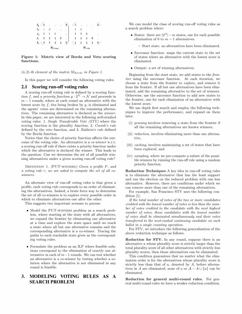
Figure 1: Matrix view of Borda and Veto scoringfunctions.

(4, 2)-th element of the matrix MBorda in Figure 1.

In this paper we will consider the following voting rules.

2.1 Scoring run-off voting rulesA scoring run-off voting rule is defined by a scoring func-

tion f , and a priority function g : 2N → N and proceeds inm− 1 rounds, where at each round an alternative with thelowest score by f , ties being broken by g, is eliminated andthe agents’ votes are determined on the remaining alterna-tives. The remaining alternative is declared as the winner.In this paper, we are interested in the following well-studiedvoting rules: 1. Single Transferable Vote (STV) where thescoring function is the plurality function, 2. Coomb’s ruledefined by the veto function, and 3. Baldwin’s rule definedby the Borda function.

Notice that the choice of priority function affects the out-come of the voting rule. An alternative is a co-winner w.r.t.a scoring run-off rule if there exists a priority function underwhich the alternative is declared the winner. This leads tothe question: Can we determine the set of all possible win-ning alternatives under a given scoring run-off voting rule?

Definition 1. (PUT-winners) Given a profile P , anda voting rule r, we are asked to compute the set of all co-winners.

An alternate view of run-off voting rules is that given aprofile, each voting rule corresponds to an order of eliminat-ing the alternatives. Indeed, a brute force way to determinethe set of all co-winners is to explore every possible order inwhich to eliminate alternatives one after the other.

This suggests two important avenues to pursue:

• Model the PUT-winners problem as a search prob-lem, where starting at the state with all alternatives,we expand the frontier by eliminating one alternativeat a time and explore the state space until we reacha state where all but one alternative remains and thecorresponding alternative is a co-winner. Tracing thepaths to each reachable state gives us the correspond-ing voting rules.

• Formulate the problem as an ILP where feasible solu-tions correspond to the elimination of exactly one al-ternative in each of m−1 rounds. We can test whetheran alternative is a co-winner by testing whether a so-lution where the alternative is not eliminated in anyround is feasible.

3. MODELING VOTING RULES AS ASEARCH PROBLEM

We can model the class of scoring run-off voting rules asa search problem where:

• States: there are |2A|−m states, one for each possibleelimination of 0 to m− 1 alternatives.

– Start state: no alternatives have been eliminated.

• Successor function: maps the current state to the setof states where an alternative with the lowest score iseliminated.

• Output: a set of winning alternatives.

Beginning from the start state, we add states to the fron-tier using the successor function. At each iteration, wechoose a state from the frontier to explore, and remove itfrom the frontier. If all but one alternatives have been elim-inated, add the remaining alternative to the set of winners.Otherwise, use the successor function to add new states tothe frontier, one for each elimination of an alternative withthe lowest score.

We use depth first search and employ the following tech-niques to improve the performance, and expand on themlater.

(i) pruning involves removing a state from the frontier ifall the remaining alternatives are known winners,

(ii) reduction, involves eliminating more than one alterna-tive,

(iii) caching, involves maintaining a set of states that havebeen explored, and

(iv) sampling, where we pre-compute a subset of the possi-ble winners by running the run-off rule using a randompriority function.

Reduction Techniques A key idea in run-off voting rulesis to eliminate the alternative that has the least supportand run the election on the reduced problem with one lessalternative. However, there are conditions under which wecan remove more than one of the remaining alternatives.

For example, San Francisco STV uses the following con-dition [1].

If the total number of votes of the two or more candidatescredited with the lowest number of votes is less than the num-ber of votes credited to the candidate with the next highestnumber of votes, those candidates with the lowest numberof votes shall be eliminated simultaneously and their votestransferred to the next-ranked continuing candidate on eachballot in a single counting operation.

For STV, we introduce the following generalization of theabove reduction technique as follows.

Reduction for STV. In any round, suppose there is analternative a whose plurality score is strictly larger than thetotal plurality score of all other alternatives with strictly lessplurality scores, then those alternatives can be eliminated.

This condition guarantees that no matter what the elim-ination order is for the alternatives whose plurality score isstrictly less than that of a, denoted by A, before alterna-tives in A are eliminated, none of a or A − A ∪ {a} can beeliminated.

Reduction for general multi-round rules. For gen-eral multi-round rules we have a weaker reduction condition.

Given a collection of scoring vectors M = (~s1, . . . , ~sm), andm∗ ≤ m and any k ≤ m∗ − 2, let DiffM (P,m∗, k) denotethe maximum reduction in the score difference between apair of alternatives (a, b), before and after k alternativeshave been eliminated in a ranking over m∗ alternatives.DiffM (P,m∗, k) can be computed in polynomial time by enu-merating all positions of a and b and all ways to eliminate kalternatives (there are no more than k∗ ways, each of whichcorresponds to the number of eliminated alternatives thatare ranked higher than a and b, between a and b, and aftera and b, respectively).

The condition for general multi-round rule with scoringvectors M is: in any round, suppose there exists an alterna-tive a with score s, let s′ denote the next highest score andlet A denote the alternatives whose scores are strictly lessthan s. If s−s′ > n×DiffM (P,m∗, |A|), then all alternativesin A can be eliminated.

It is not hard to verify the correctness of the two condi-tions. The condition for STV is stronger than the genericcondition for computing PUT-STV.

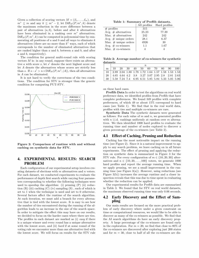
Figure 2: Comparison of runtime with and withoutcaching on synthetic data for STV.

4. EXPERIMENTAL RESULTS: SEARCHPROBLEM

Each configuration of our experimental setup involves cre-ating datasets of elections with m alternatives and n voters.For each dataset, we conducted experiments to evaluate theperformance of depth first search while varying four parame-ters corresponding to whether the following techniques wereused to speedup the algorithm: (i) pruning (P) (ii) reduc-tion (R) (iii) caching (C) (iv) sampling (S) , each of which isset to 1 when the technique is used and set to 0 otherwise.Several factors affect the runtime of the search algorithm.At each iteration, we must add a branch for every alterna-tive that is tied with the lowest score. It is easy to see howthe number of ties encountered during the running of the al-gorithm leads to an increase in the size of the search space.In order to mitigate the effect this may have on our results,we decided to focus on the harder cases where there are ties.The profiles in each dataset are marked as (i) easy if thereis a unique winner and every round has a unique alternativewith the lowest score, and (ii) hard if at some round of thevoting rule we encounter more than one alternative tied withthe lowest score. We will focus on results for the STV rule

Table 1: Summary of Preflib datasets.All profiles Hard profiles

# profiles 315 49Avg. # alternatives 25.23 77.39Max. # alternatives 242 242Avg. # unique orders 28.1 6.37Max. # unique orders 4926 30Avg. # co-winners 1.1 1.67Max. # co-winners 4 4

Table 2: Average number of co-winners for syntheticdatasets

nm 10 20 30 40 50 60 70 80 90 10010 2.89 2.04 1.88 1.78 1.72 1.64 1.57 1.58 1.53 1.5320 4.65 4.64 4.2 3.8 3.27 3.07 2.95 2.8 2.81 2.6330 5.58 7.24 7.4 6.95 6.51 5.85 5.84 5.33 5.05 5.06

on these hard cases.Preflib Data In order to test the algorithms on real world

preference data, we identified profiles from Preflib that havecomplete preferences. We found 349 profiles with completepreferences, of which 49 or about 15% correspond to hardcases (see Table 1). We find that in the real world data,profiles with ties and multiple co-winners are rare.

Synthetic Data The synthetic datasets were generatedas follows: For each value of m and n, we generated profileswith n i.i.d. rankings uniformly at random over m alterna-tives. We then identified 1000 hard profiles to evaluate therunning time and number of nodes explored to discover agiven percentage of the co-winners (see Table 2).

4.1 Effect of Caching, Pruning and ReductionCaching has the most noticeable impact on the running

time (see Figure 2). Since it is a natural improvement to ap-ply to any search problem, we leave caching on in all futureexperiments. The effect of pruning and applying the reduc-tion on synthetic data is summarized in Figure 3 for theSTV rule. For every configuration of m ∈ {10, 20, 30} alter-natives and n ∈ {10, 20, . . . , 100} voters, we generate 1000hard profiles and report the average running time. Whenwe apply pruning, we see a small improvement in the run-ning time (see Figure 3(a)). However, using reductions (seeFigure 3(b)) increases the average runtime and a closer in-spection reveals that this was due to time spent in evaluatingwhether the reduction can be applied.

Our experimental results for Preflib data are summarizedin Table 3. We found that for STV on real world datasets,the maximum observed running time was only 0.06 seconds.

4.2 Early Discovery and the Effect of Sam-pling

Our main results are focused on the more practical prob-lem of early discovery where under a given constraint ontime or computational resources, we would like to be able todiscover as many of the co-winners as possible. We find thatthe AI search algorithms do have an early discovery prop-erty. A large percentage of the co-winners are found earlyin the exploration. For m = 20, we find that close to 80% ofthe co-winners are discovered after exploring just 200 statesand for m = 30, close to half of all the co-winners are dis-

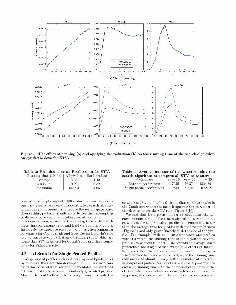
Figure 3: The effect of pruning (a) and applying the reduction (b) on the running time of the search algorithmon synthetic data for STV.

Table 3: Running time on Preflib data for STV.Running time (10−4s) All profiles Hard profiles

average 3.35 1.42minimum 0.39 0.52maximum 648.93 4.65

covered after exploring only 100 states. Somewhat unsur-prisingly even a relatively unsophisticated search strategywithout any improvements to reduce the search space otherthan caching performs significantly better than attemptingto discover co-winners by breaking ties at random.

For comparison, we include the running time of the searchalgorithms for Coomb’s rule and Baldwin’s rule in Figure 5.Intuitively, we expect to see a lot more ties when computingco-winners for Coomb’s rule and fewer ties for Baldwin’s ruleand we can observe its effect on the running times which arelarger than STV in general for Coomb’s rule and significantlylower for Baldwin’s rule.

4.3 AI Search for Single Peaked ProfilesWe generated profiles with i.i.d. single-peaked preferences

by following the algorithm developed in [15]. For each con-figuration of m alternatives and n candidates, we identified500 hard profiles from a set of randomly generated profiles.Most of the profiles have either a unique winner or only few

Table 4: Average number of ties when running thesearch algorithm to compute all STV co-winners.

Preferences m = 10 m = 20 m = 30Random preferences 4.7255 76.574 1324.301

Single-peaked preferences 1.9354 3.7466 6.4802

co-winners (Figure 6(a)) and the median candidate (who isthe Condorcet winner) is most frequently the co-winner ofthe election under the STV rule (Figure 6(b)).

We find that for a given number of candidates, the av-erage running time of the search algorithm to compute allco-winners for single peaked profiles is significantly fasterthan the average time for profiles with random preferences(Figure 7) and only grows linearly with the size of the pro-file. For example, with m = 30 alternatives and profileswith 100 voters, the running time of the algorithm to com-pute all co-winners is under 0.003 seconds on average whenpreferences are single peaked which is 2 orders of magni-tude lower than the average runtime for random preferenceswhich is close to 0.2 seconds. Indeed, while the running timeonly increased almost linearly with the number of voters forsingle-peaked preferences, we observe a near exponential in-crease in running time with the number of candidates in theelection when profiles have random preferences. This is notsurprising when we consider the number of ties encountered

Figure 4: Early discovery of co-winners on synthetic data for STV.

(a) Coomb’s rule.

(b) Baldwin’s rule.

Figure 5: Running time of the search algorithm on synthetic data with and without pruning for the Coomb’sand Baldwin’s rules.

on average by the search algorithm as shown in Table 4.

5. ILP FORMULATIONWe model the PUT-winners problem as an ILP where

the solutions correspond to the elimination of a single alter-native in each of m− 1 rounds and we test whether a givenalternative is the co-winner by checking if there is a feasiblesolution when we enforce the constraint that the given al-ternative is not eliminated in any of the rounds. We presentILP formulations of the STV and Baldwin’s voting rules be-low. The ILP for Coomb’s rule is similar to the ILP for STVwhere the scoring rule is changed from plurality to veto. Foreach alternative ai ∈ A, and for each round t ≤ m − 1, we

define the variable xti ∈ {0, 1} to model the elimination of

ai at round t.

Table 5: ILP for STV rule.m n Profiles ILP

alternativesUncertain

alternativesRuntime(s)

10 10 392 6.51 3.52 13.02610 20 104 8.71 6.91 961.6410 30 88 9.10 7.49 1799.8220 10 224 7.93 3.34 177.3120 20 4 12.25 12 4438.66

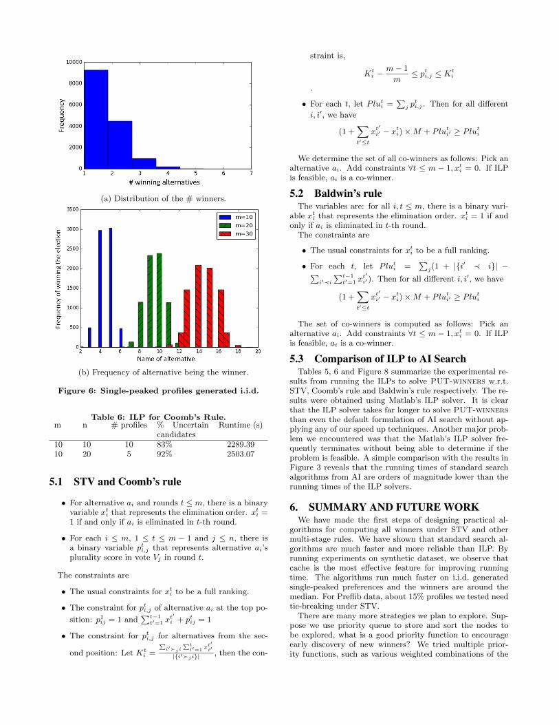
(a) Distribution of the # winners.

(b) Frequency of alternative being the winner.

Figure 6: Single-peaked profiles generated i.i.d.

Table 6: ILP for Coomb’s Rule.m n # profiles % Uncertain

candidatesRuntime (s)

10 10 10 83% 2289.3910 20 5 92% 2503.07

5.1 STV and Coomb’s rule

• For alternative ai and rounds t ≤ m, there is a binaryvariable xt

i that represents the elimination order. xti =

1 if and only if ai is eliminated in t-th round.

• For each i ≤ m, 1 ≤ t ≤ m − 1 and j ≤ n, there isa binary variable pti,j that represents alternative ai’splurality score in vote Vj in round t.

The constraints are

• The usual constraints for xti to be a full ranking.

• The constraint for pti,j of alternative ai at the top po-

sition: p1ij = 1 and∑t−1

t′=1 xt′i + ptij = 1

• The constraint for pti,j for alternatives from the sec-

ond position: Let Kti =

∑i′�ji

∑tt′=1

xt′i′

|{i′�ji}|, then the con-

straint is,

Kti −

m− 1

m≤ pti,j ≤ Kt

i

.

• For each t, let Pluti =

∑j p

ti,j . Then for all different

i, i′, we have

(1 +∑t′≤t

xt′i′ − xt

i)×M + Pluti′ ≥ Plut

i

We determine the set of all co-winners as follows: Pick analternative ai. Add constraints ∀t ≤ m − 1, xt

i = 0. If ILPis feasible, ai is a co-winner.

5.2 Baldwin’s ruleThe variables are: for all i, t ≤ m, there is a binary vari-

able xti that represents the elimination order. xt

i = 1 if andonly if ai is eliminated in t-th round.

The constraints are

• The usual constraints for xti to be a full ranking.

• For each t, let Pluti =

∑j(1 + |{i′ ≺ i}| −∑

i′≺i

∑t−1t′=1 x

t′

i′ ). Then for all different i, i′, we have

(1 +∑t′≤t

xt′

i′ − xti)×M + Plut

i′ ≥ Pluti

The set of co-winners is computed as follows: Pick analternative ai. Add constraints ∀t ≤ m − 1, xt

i = 0. If ILPis feasible, ai is a co-winner.

5.3 Comparison of ILP to AI SearchTables 5, 6 and Figure 8 summarize the experimental re-

sults from running the ILPs to solve PUT-winners w.r.t.STV, Coomb’s rule and Baldwin’s rule respectively. The re-sults were obtained using Matlab’s ILP solver. It is clearthat the ILP solver takes far longer to solve PUT-winnersthan even the default formulation of AI search without ap-plying any of our speed up techniques. Another major prob-lem we encountered was that the Matlab’s ILP solver fre-quently terminates without being able to determine if theproblem is feasible. A simple comparison with the results inFigure 3 reveals that the running times of standard searchalgorithms from AI are orders of magnitude lower than therunning times of the ILP solvers.

6. SUMMARY AND FUTURE WORKWe have made the first steps of designing practical al-

gorithms for computing all winners under STV and othermulti-stage rules. We have shown that standard search al-gorithms are much faster and more reliable than ILP. Byrunning experiments on synthetic dataset, we observe thatcache is the most effective feature for improving runningtime. The algorithms run much faster on i.i.d. generatedsingle-peaked preferences and the winners are around themedian. For Preflib data, about 15% profiles we tested needtie-breaking under STV.

There are many more strategies we plan to explore. Sup-pose we use priority queue to store and sort the nodes tobe explored, what is a good priority function to encourageearly discovery of new winners? We tried multiple prior-ity functions, such as various weighted combinations of the

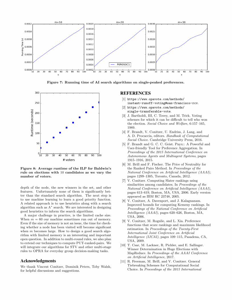
Figure 7: Running time of AI search algorithms on single-peaked preferences.

Figure 8: Average runtime of the ILP for Baldwin’srule on elections with 10 candidates as we vary thenumber of voters.

depth of the node, the new winners in the set, and otherfeatures. Unfortunately none of them is significantly bet-ter than the standard search algorithm. The next step isto use machine learning to learn a good priority function.A related approach is to use heuristics along with a searchalgorithm such as A∗ search. We are interested in designinggood heuristics to inform the search algorithms.

A major challenge in practice, is the limited cache size.When m = 60 our machine sometimes run out of memory.Even if the size of memory is not an issue, the time for check-ing whether a node has been visited will become significantwhen m becomes large. How to design a good search algo-rithm with limited memory is an interesting and importantopen question. In addition to multi-round rules, we also planto extend our techniques to compute PUT-ranked-pairs. Wewill integrate our algorithms for STV and other multi-stagerules to OPRA for everyday group decision-making tasks.

AcknowledgmentsWe thank Vincent Conitzer, Dominik Peters, Toby Walsh,for helpful discussions and suggestions.

REFERENCES[1] https://www.opavote.com/methods/

instant-runoff-voting#san-francisco-rcv.

[2] https://www.opavote.com/methods/

single-transferable-vote.

[3] J. Bartholdi, III, C. Tovey, and M. Trick. Votingschemes for which it can be difficult to tell who wonthe election. Social Choice and Welfare, 6:157–165,1989.

[4] F. Brandt, V. Conitzer, U. Endriss, J. Lang, andA. D. Procaccia, editors. Handbook of ComputationalSocial Choice. Cambridge University Press, 2016.

[5] F. Brandt and G. C. C. Geist. Pnyx:: A Powerful andUser-friendly Tool for Preference Aggregation. InProceedings of the 2015 International Conference onAutonomous Agents and Multiagent Systems, pages1915–1916, 2015.

[6] M. Brill and F. Fischer. The Price of Neutrality forthe Ranked Pairs Method. In Proceedings of theNational Conference on Artificial Intelligence (AAAI),pages 1299–1305, Toronto, Canada, 2012.

[7] V. Conitzer. Computing Slater rankings usingsimilarities among candidates. In Proceedings of theNational Conference on Artificial Intelligence (AAAI),pages 613–619, Boston, MA, USA, 2006. Early versionappeared as IBM RC 23748, 2005.

[8] V. Conitzer, A. Davenport, and J. Kalagnanam.Improved bounds for computing Kemeny rankings. InProceedings of the National Conference on ArtificialIntelligence (AAAI), pages 620–626, Boston, MA,USA, 2006.

[9] V. Conitzer, M. Rognlie, and L. Xia. Preferencefunctions that score rankings and maximum likelihoodestimation. In Proceedings of the Twenty-FirstInternational Joint Conference on ArtificialIntelligence (IJCAI), pages 109–115, Pasadena, CA,USA, 2009.

[10] T. Csar, M. Lackner, R. Pichler, and E. Sallinger.Winner Determination in Huge Elections withMapReduce. In Proceedings of the AAAI Conferenceon Artificial Intelligence, 2017.

[11] R. Freeman, M. Brill, and V. Conitzer. GeneralTiebreaking Schemes for Computational SocialChoice. In Proceedings of the 2015 International

Conference on Autonomous Agents and MultiagentSystems, pages 1401–1409, 2015.

[12] C. Kenyon-Mathieu and W. Schudy. How to Rankwith Few Errors: A PTAS for Weighted Feedback ArcSet on Tournaments. In Proceedings of theThirty-ninth Annual ACM Symposium on Theory ofComputing, pages 95–103, San Diego, California, USA,2007.

[13] N. Mattei, N. Narodytska, and T. Walsh. How hard isit to control an election by breaking ties? InProceedings of the Twenty-first European Conferenceon Artificial Intelligence, pages 1067–1068, 2014.

[14] P. Stone, R. Brooks, E. Brynjolfsson, R. Calo,O. Etzioni, G. Hager, J. Hirschberg,S. Kalyanakrishnan, E. Kamar, S. Kraus,K. Leyton-Brown, D. Parkes, W. Press, A. Saxenian,J. Shah, M. Tambe, and A. Teller. Artificialintelligence and life in 2030. One Hundred Year Studyon Artificial Intelligence: Report of the 2015-2016Study Panel, Stanford University, Stanford, CA,September 2016.

[15] T. Walsh. Generating single peaked votes. arXivpreprint arXiv:1503.02766, 2015.