A practical tour of optimization algorithms for the Lasso · A practical tour of optimization...

Alexandre [email protected]

Inria, Parietal TeamUniversité Paris-Saclay

A practical tour of optimization algorithms for the Lasso

Huawei - Apr. 2017

mailto:[email protected]?subject=

Alex Gramfort Algorithms for the Lasso

Outline

2

• What is the Lasso

• Lasso with an orthogonal design

• From projected gradient to proximal gradient

• Optimality conditions and subgradients (LARS algo.)

• Coordinate descent algorithm

… with some demos


Lasso

3

with

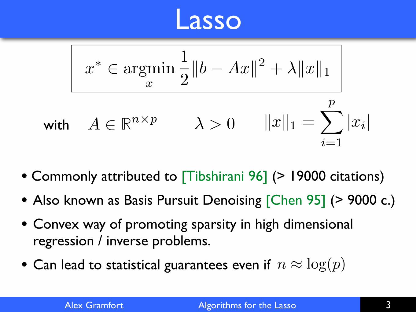
• Commonly attributed to [Tibshirani 96] (> 19000 citations)

• Also known as Basis Pursuit Denoising [Chen 95] (> 9000 c.)

• Convex way of promoting sparsity in high dimensional regression / inverse problems.

• Can lead to statistical guarantees even if n ⇡ log(p)

� > 0 kxk1 =pX

i=1

|xi|A 2 Rn⇥p

x

⇤ 2 argminx

1

2kb�Axk2 + �kxk1


Algorithm 0

4

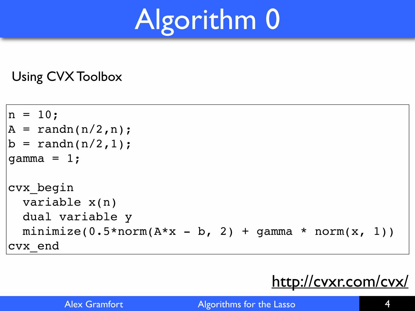
http://cvxr.com/cvx/

n = 10;A = randn(n/2,n);b = randn(n/2,1);gamma = 1;

cvx_begin variable x(n) dual variable y minimize(0.5*norm(A*x - b, 2) + gamma * norm(x, 1))cvx_end

Using CVX Toolbox

http://cvxr.com/cvx/


Algorithm 1

5

Rewrite:

|xi| = x

+i � x

�i = max(xi, 0) + max(�xi, 0)

kxk1 = x

+ � x

�

xi = x

+i + x

�i = max(xi, 0) + min(xi, 0)

Leads to:

• This is a simple smooth convex optimization problem with positivity constraints (convex constraints)

z⇤ 2 argminz2R2p

+

1

2kb� [A,�A]zk2 + �

X

i

zi


Gradient Descent

6

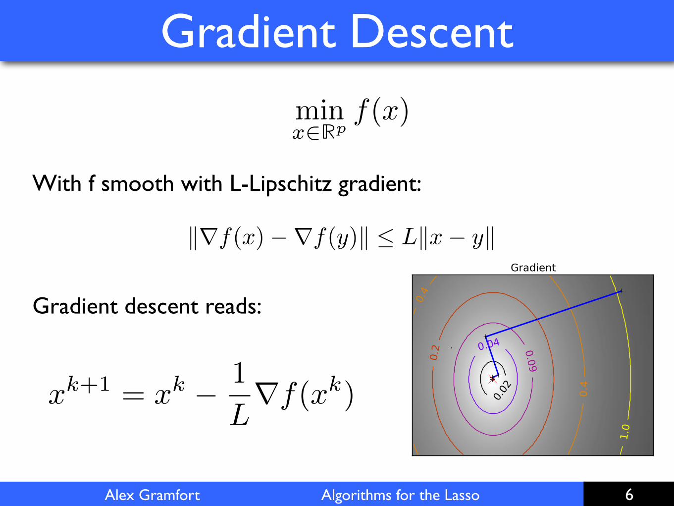
With f smooth with L-Lipschitz gradient:

x

k+1 = x

k � 1

L

rf(xk)

minx2Rp

f(x)

krf(x)�rf(y)k Lkx� yk

Gradient descent reads:


Projected gradient Descent

7

minx2C⇢Rp

f(x)

With a convex set and f smooth with L-Lipschitz gradientC

x

k+1 = ⇡C(xk � 1

L

rf(xk))

C⇡C(x)

x

projected gradient reads:

Orthogonal projection on C

demo_grad_proj.ipynb


What if A is orthogonal?

9

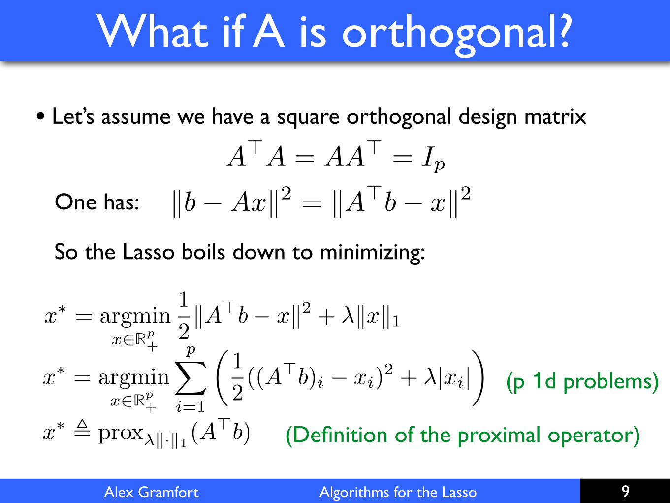
• Let’s assume we have a square orthogonal design matrix

One has:

A>A = AA> = Ip

kb�Axk2 = kA>b� xk2

So the Lasso boils down to minimizing:

x

⇤ = argminx2Rp

+

1

2kA>

b� xk2 + �kxk1

x

⇤ = argminx2Rp

+

pX

i=1

✓1

2((A>

b)i

� x

i

)2 + �|xi

|◆

(p 1d problems)

x

⇤ , prox�k·k1(A

>b) (Definition of the proximal operator)


Proximal operator of L1 norm

10SEPTEMBER 2011R. GRIBONVAL - SPARSE METHODS - MLSS 2011

Soft-thresholding (p=1)

• Solution of

�

��

13

S�(c)

c

minx

12(c� x)2 + � · |x|

is the solution of

The soft-thresholding: c ! sign(c)(|c|� �)+


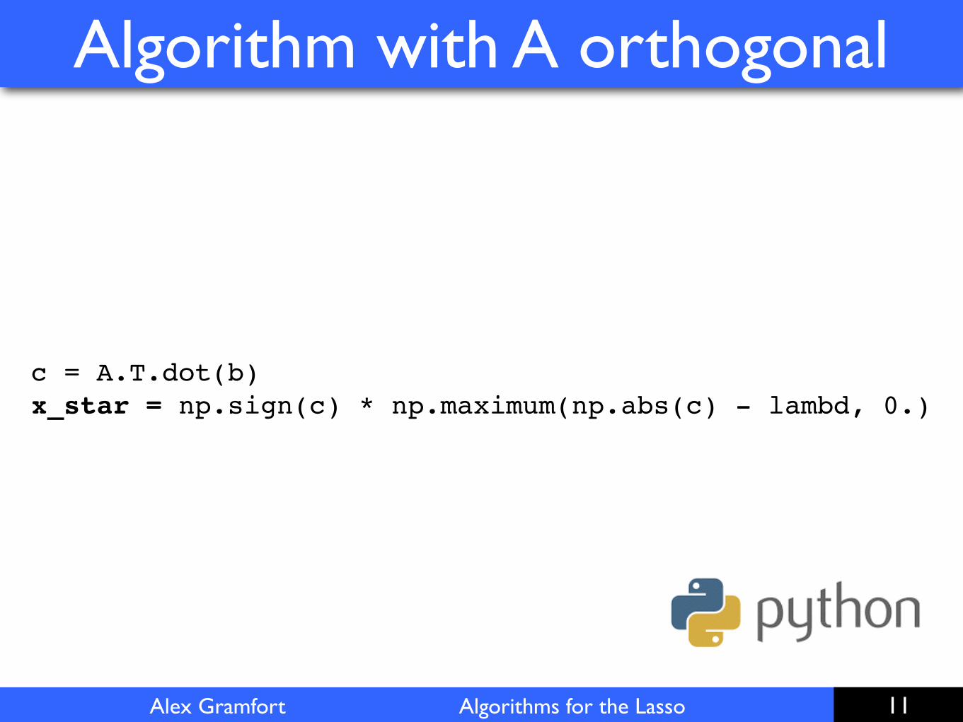
Algorithm with A orthogonal

11

c = A.T.dot(b)x_star = np.sign(c) * np.maximum(np.abs(c) - lambd, 0.)


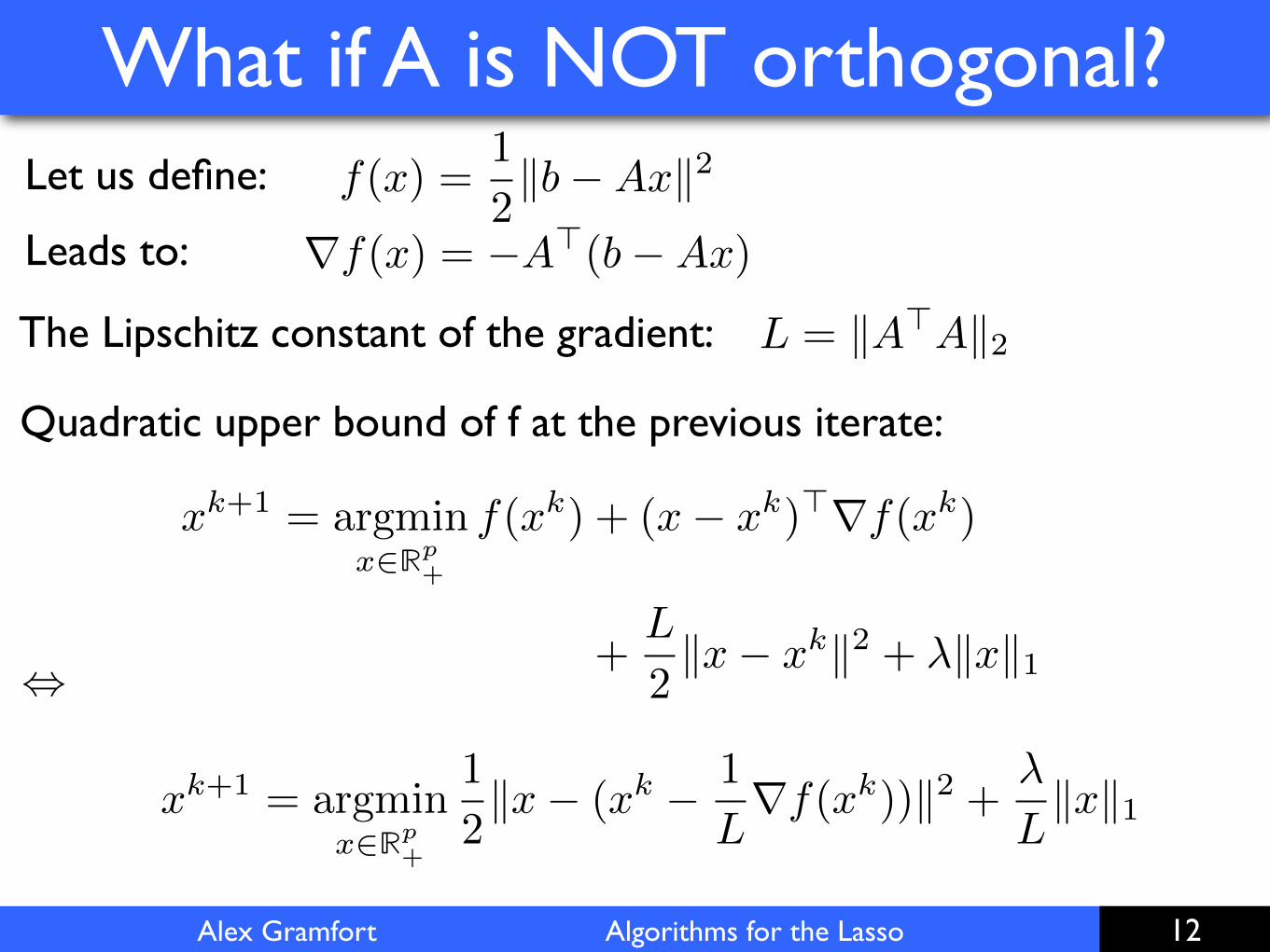
What if A is NOT orthogonal?

12

Let us define:

Leads to:

The Lipschitz constant of the gradient:

f(x) =1

2kb�Axk2

rf(x) = �A

>(b�Ax)

L = kA>Ak2

Quadratic upper bound of f at the previous iterate:

,

x

k+1 = argminx2Rp

+

f(xk) + (x� x

k)>rf(xk)

+L

2kx� x

kk2 + �kxk1

x

k+1 = argminx2Rp

+

1

2kx� (xk � 1

L

rf(xk))k2 + �

L

kxk1


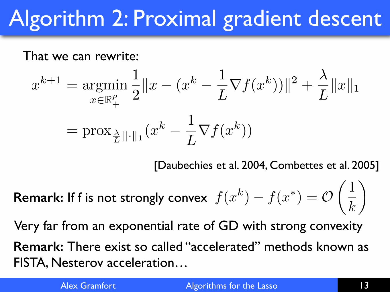
Algorithm 2: Proximal gradient descent

13

That we can rewrite:

x

k+1= argmin

x2Rp+

1

2

kx� (x

k � 1

L

rf(x

k

))k2 + �

L

kxk1

= prox �Lk·k1

(x

k � 1

L

rf(x

k

))

[Daubechies et al. 2004, Combettes et al. 2005]

Remark: There exist so called “accelerated” methods known as FISTA, Nesterov acceleration…

Remark: If f is not strongly convex f(xk)� f(x⇤) = O✓1

k

◆

Very far from an exponential rate of GD with strong convexity


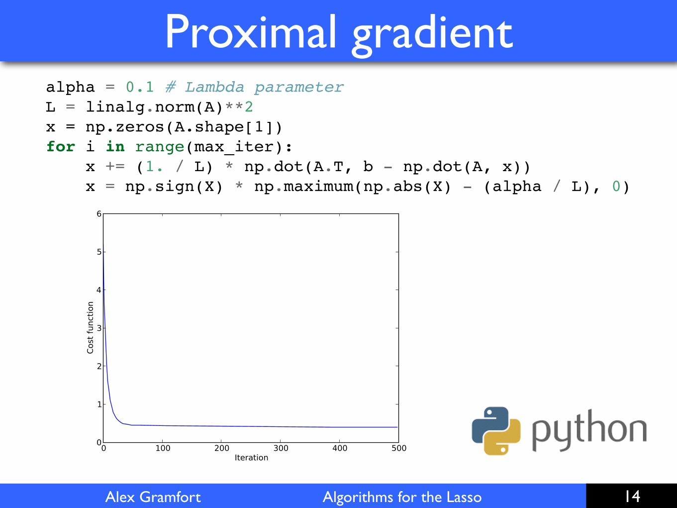
Proximal gradient

14

alpha = 0.1 # Lambda parameterL = linalg.norm(A)**2x = np.zeros(A.shape[1])for i in range(max_iter): x += (1. / L) * np.dot(A.T, b - np.dot(A, x)) x = np.sign(X) * np.maximum(np.abs(X) - (alpha / L), 0)

demo_grad_proximal.ipynb


Pros of proximal gradient

16

• First order method (only requires to compute gradients)

• Algorithms scalable even if p is large (needs to store A in

memory)

• Great if A is an implicit linear operator (Fourier, Wavelet, MDCT,

etc.) as dot products have some logarithmic complexities.


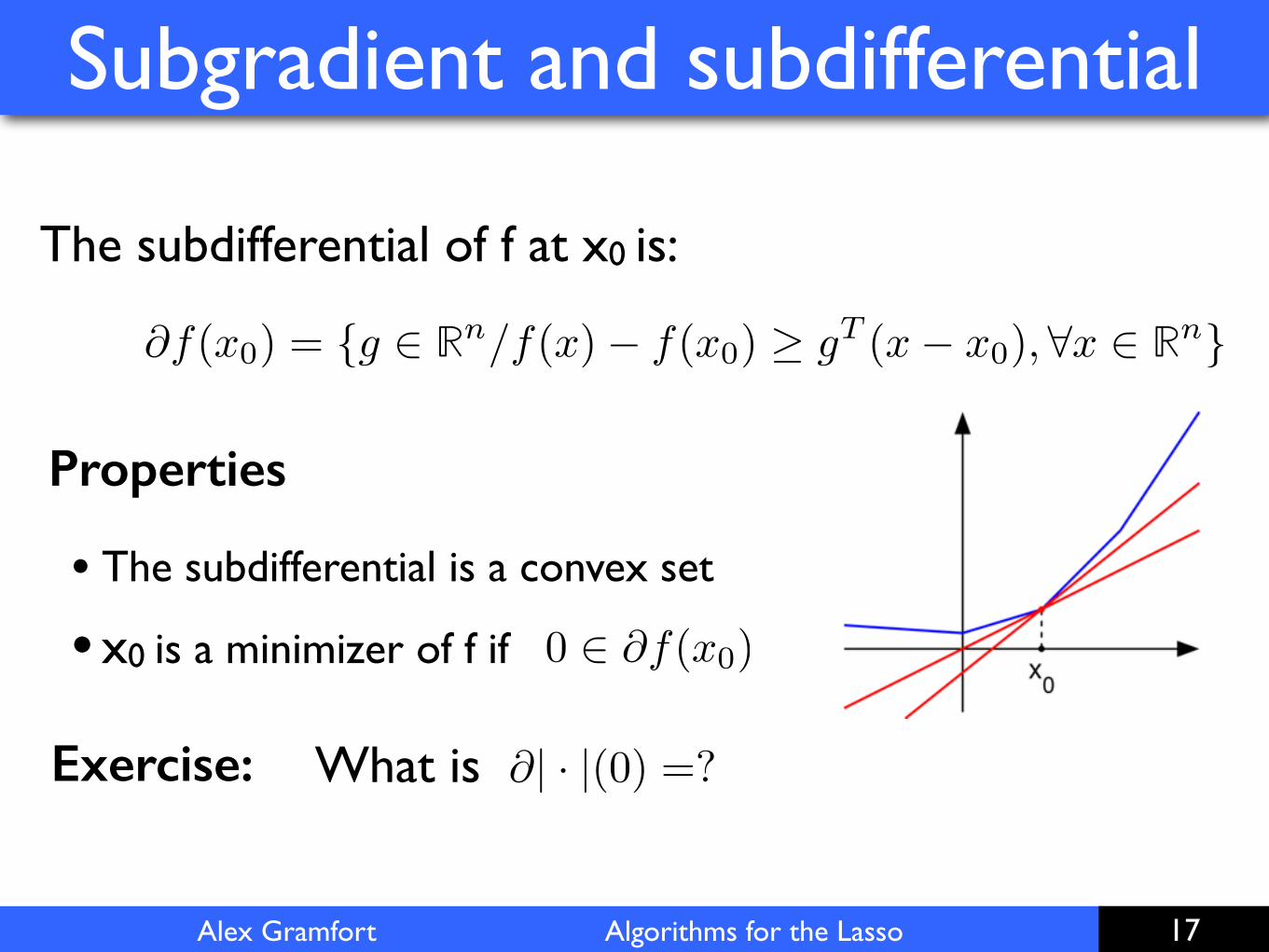
Subgradient and subdifferential

17

The subdifferential of f at x0 is:

@f(x0) = {g 2 Rn/f(x)� f(x0) � g

T (x� x0), 8x 2 Rn}

Properties

• The subdifferential is a convex set

• x0 is a minimizer of f if 0 2 @f(x0)

@| · |(0) =?What is Exercise:


Path of solutions

18

Lemma [Fuchs 97] : Let be a solution of the Lasso

x

⇤ 2 argminx

1


x

⇤ 2 argminx

1


I = {i s.t. xi 6= 0}Let the support

Then:A

>I (Ax

⇤ � b) + � sign(x⇤I) = 0

kA>Ic(Ax

⇤ � b)k1 �

x

⇤I = (A>

I AI)�1(A>

I b� � sign(x⇤I))

And also:


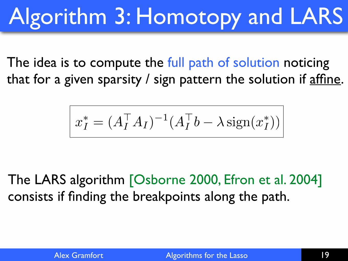
Algorithm 3: Homotopy and LARS

19

x

⇤I = (A>

I AI)�1(A>

I b� � sign(x⇤I))

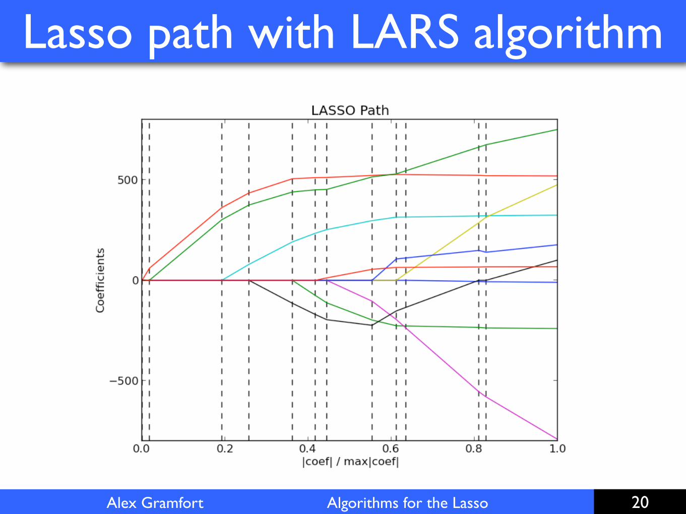
The idea is to compute the full path of solution noticing that for a given sparsity / sign pattern the solution if affine.

The LARS algorithm [Osborne 2000, Efron et al. 2004] consists if finding the breakpoints along the path.


Lasso path with LARS algorithm

20


Pros/Cons of LARS

21

• Gives the full path of solution

• Fast with support is small and one can compute Gram matrix

• Scales with the size of the support

• Hard to make it numerically stable

• One can have many many breakpoints [Mairal et al. 2012]

Pros:

Cons:

demo_lasso_lars.ipynb


Coordinate descent (CD)

23

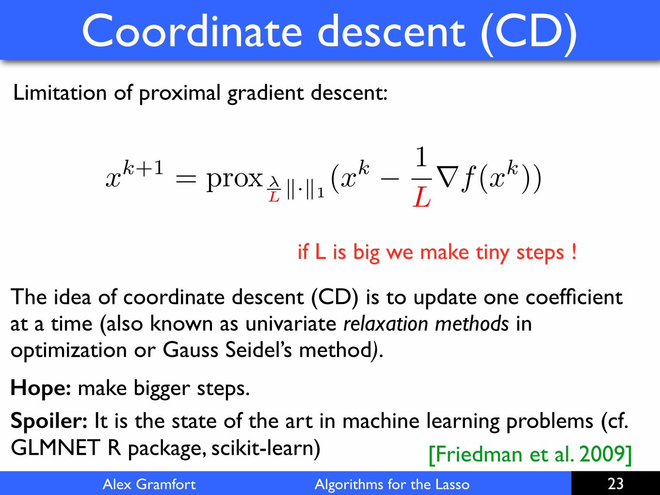
Limitation of proximal gradient descent:

if L is big we make tiny steps !

x

k+1= prox �

Lk·k1(x

k � 1

L

rf(x

k))

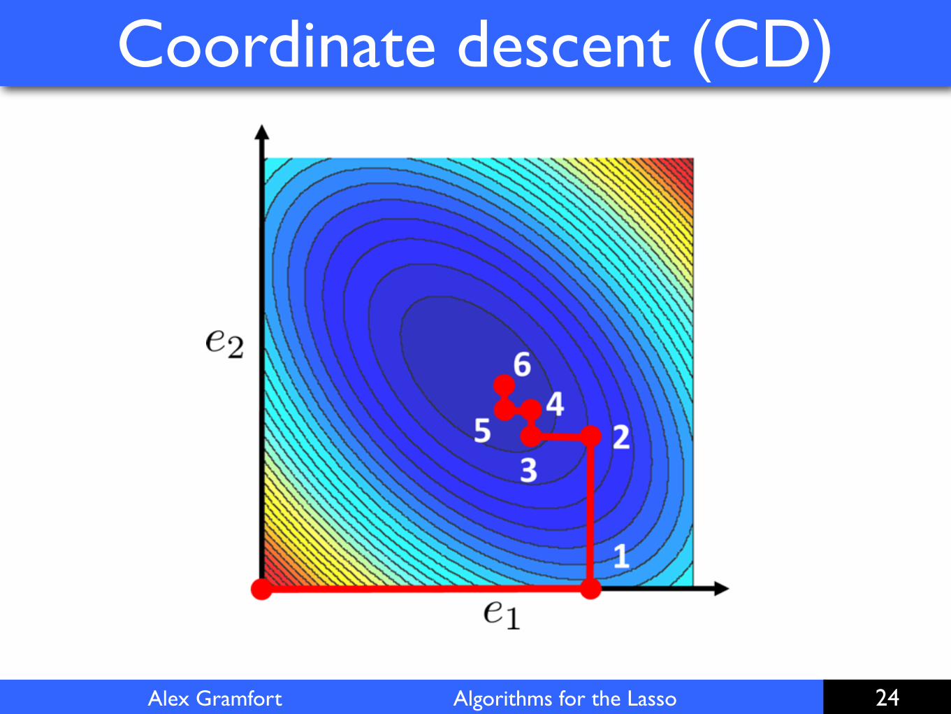
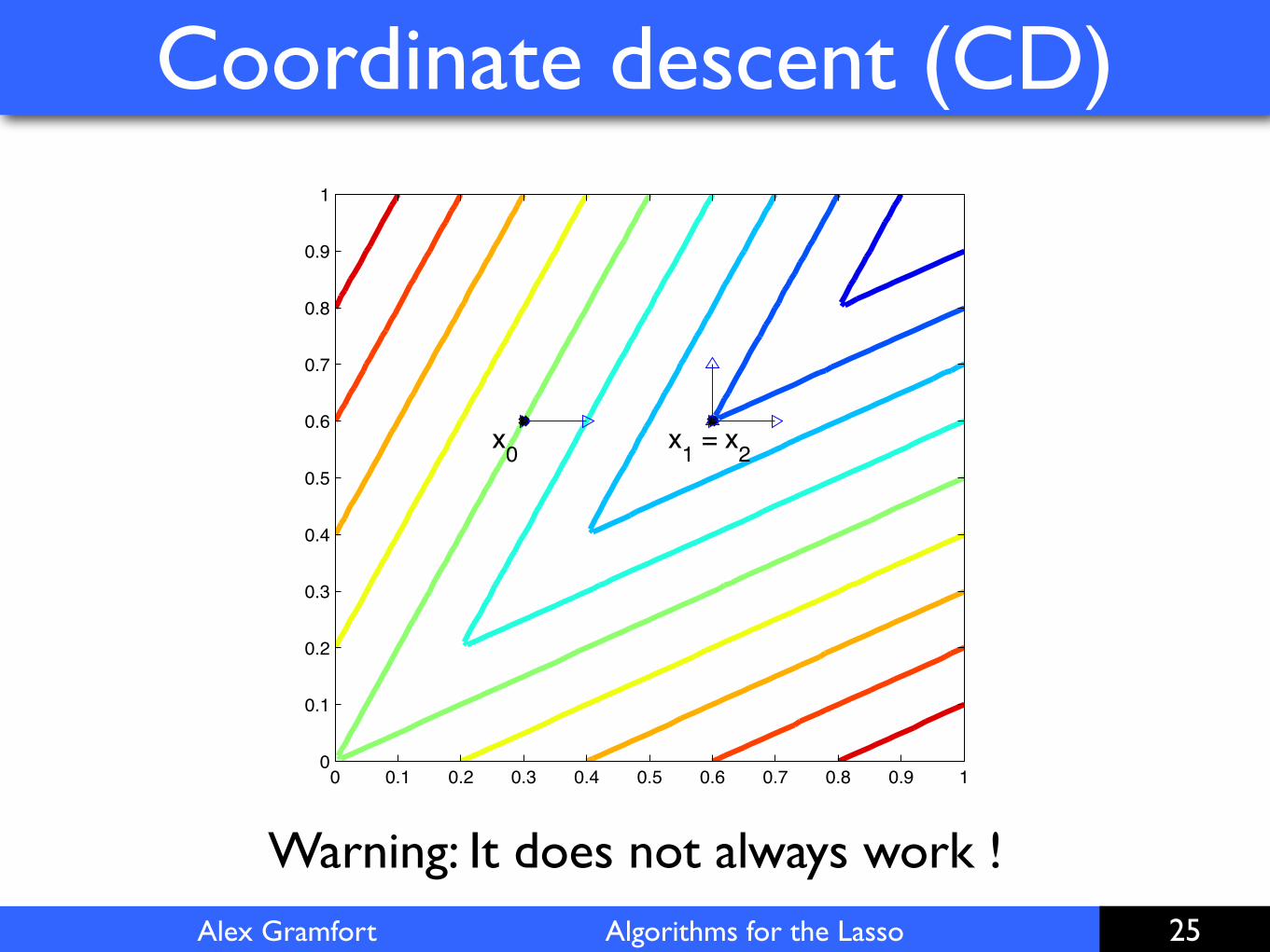
The idea of coordinate descent (CD) is to update one coefficient at a time (also known as univariate relaxation methods in optimization or Gauss Seidel’s method).

Hope: make bigger steps.Spoiler: It is the state of the art in machine learning problems (cf. GLMNET R package, scikit-learn) [Friedman et al. 2009]



24



25

x0 x1 = x2

0 0.1 0.2 0.3 0.4 0.5 0.6 0.7 0.8 0.9 10

0.1

0.2

0.3

0.4

0.5

0.6

0.7

0.8

0.9

1

Warning: It does not always work !


Algorithm 4: Coordinate descent (CD)

26

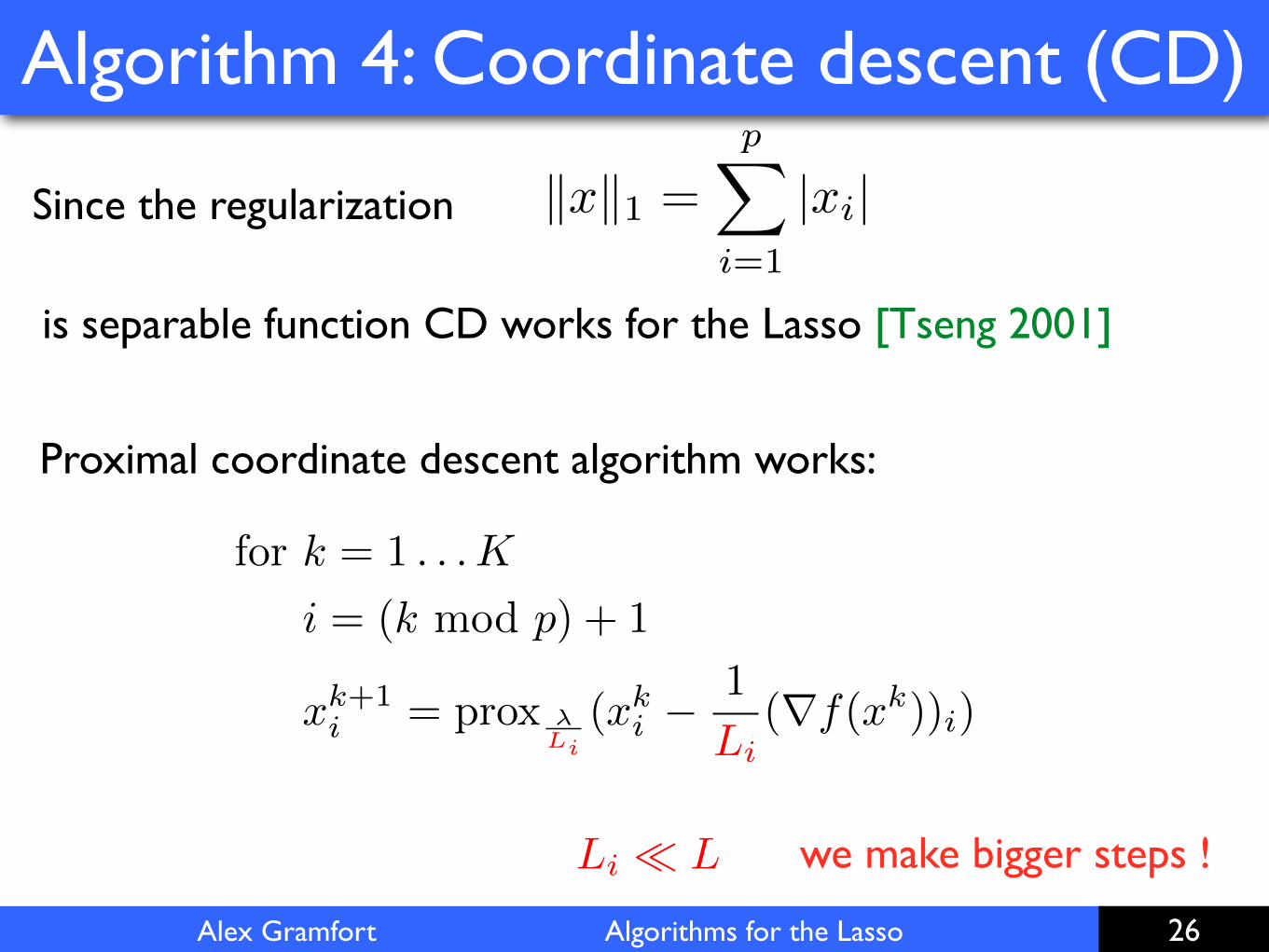
Since the regularization kxk1 =pX

i=1

|xi|

is separable function CD works for the Lasso [Tseng 2001]

Proximal coordinate descent algorithm works:

we make bigger steps !Li ⌧ L

for k = 1 . . .K

i = (k mod p) + 1

x

k+1i = prox �

Li

(x

ki � 1

Li(rf(x

k))i)


Algorithm 4: Coordinate descent (CD)

27

• Their exist many “tricks” to make CD fast for the Lasso

• Lazy update of the residuals

• Pre-computation of certain dot products

• Active set methods

• Screening rules

• More in the next talk…


Conclusion

28

• What is the Lasso

• Lasso with an orthogonal design

• From projected gradient to proximal gradient

• Optimality conditions and subgradients (LARS algo.)

• Coordinate descent algorithm

GitHub : @agramfort Twitter : @agramfort

http://alexandre.gramfort.netContact

A practical tour of optimization algorithms for the Lasso · A practical tour of optimization...

Documents

Transcript of A practical tour of optimization algorithms for the Lasso · A practical tour of optimization...