Power System Voltage Stability and Models of Devices

Chapter 2Power System Voltage Stability and Modelsof Devices

Abstract This chapter introduces the concepts of voltage instability and thedistinctions between voltage and angle instability. The driving force and main causesof voltage instability are analysed. Different methods and devices used to enhancevoltage stability are also explained. The steady-state and dynamic modelling of thepower system devices including wind generators and photovoltaic units have beendiscussed.

2.1 Introduction

Power systemstability has been recognised as an important problem for secure systemoperation since the beginning of last century. Many major blackouts caused due topower system instability have illustrated the importance of this phenomenon [1, 2].Angle stability had been the primary concern of the utilities for many decades. How-ever, in the last two decades power systems have operated under much more stressedconditions than they usually had in the past. There are number of factors responsiblefor this: continuing growth in interconnections; the use of new technologies; bulkpower transmissions over long transmission lines; environmental pressures on trans-mission expansion; increased electricity consumption in heavy load areas (where itis not feasible or economical to install new generating plants); new system loadingpatterns due to the opening up of the electricity market; growing use of inductionmachines; and large penetration of wind generators and local uncoordinated controlsin systems. Under these stressed conditions a power system can exhibit a new typeof unstable behaviour, namely, voltage instability.

In recent years, voltage instability has become a major research area in the fieldof power systems after a number of voltage instability incidents were experiencedaround the world [3, 4]. In Japan, a large-scale power failure occurred in the Tokyometropolitan area in 1987 (about an 8-GW loss) because of voltage instability [5].In Tokyo, the capacitance of 275-kV underground cables created adverse effects on

J. Hossain and H. R. Pota, Robust Control for Grid Voltage Stability: 19High Penetration of Renewable Energy, Power Systems,DOI: 10.1007/978-981-287-116-9_2, © Springer Science+Business Media Singapore 2014

20 2 Power System Voltage Stability and Models of Devices

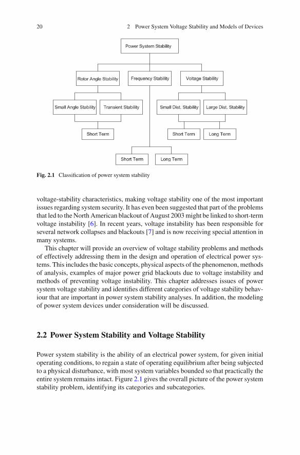
Fig. 2.1 Classification of power system stability

voltage-stability characteristics, making voltage stability one of the most importantissues regarding system security. It has even been suggested that part of the problemsthat led to theNorth American blackout of August 2003might be linked to short-termvoltage instability [6]. In recent years, voltage instability has been responsible forseveral network collapses and blackouts [7] and is now receiving special attention inmany systems.

This chapter will provide an overview of voltage stability problems and methodsof effectively addressing them in the design and operation of electrical power sys-tems. This includes the basic concepts, physical aspects of the phenomenon, methodsof analysis, examples of major power grid blackouts due to voltage instability andmethods of preventing voltage instability. This chapter addresses issues of powersystem voltage stability and identifies different categories of voltage stability behav-iour that are important in power system stability analyses. In addition, the modelingof power system devices under consideration will be discussed.

2.2 Power System Stability and Voltage Stability

Power system stability is the ability of an electrical power system, for given initialoperating conditions, to regain a state of operating equilibrium after being subjectedto a physical disturbance, with most system variables bounded so that practically theentire system remains intact. Figure 2.1 gives the overall picture of the power systemstability problem, identifying its categories and subcategories.

2.2 Power System Stability and Voltage Stability 21

The concept of voltage stability addresses a large variety of different phenomenadepending on which part of the power system is being analysed; for instance, it canbe a fast phenomenon if induction motors, air conditioning loads or high-voltage DCtransmission (HVDC) links are involved or a slow phenomenon if, for example, amechanical tap changer is involved. Today, it is well accepted that voltage instabilityis a dynamic process since it is related to dynamic loads [8, 9].

Voltage stability refers to the ability of a power system tomaintain steady voltagesat all buses in the system and maintain or restore equilibrium between load demandand load supply from its given initial operating conditions after it has been subjectedto a disturbance. Instability may result in progressive voltage falls or rises at somebuses. A possible outcome of voltage instability is the loss of load in an area, andpossible tripping of transmission lines and other elements by their protective systemswhich can lead to cascading outages.

Voltage collapse is more complex than voltage instability and is the process bywhich the sequence of events accompanying voltage instability lead to a blackout orabnormally low voltages in a significant part of a power system. The main symptomsof voltage collapse are: low voltage profiles; heavy reactive power flows; inadequatereactive support; and heavily loaded systems. The collapse is often precipitated bylow-probability single or multiple contingencies. When a power system is subjectedto a sudden increase of reactive power demand following a system contingency, theadditional demand is met by the reactive power reserves of generators and com-pensators. Generally, there are sufficient reserves and the system settles to a stablevoltage level. However, it is possible, due to a combination of events and systemconditions, that the lack of additional reactive power may lead to voltage collapse,thereby causing a total or partial breakdown of the system.

2.3 Voltage and Angle Instability

Power system instability is essentially a single problem; however, the various formsof instability that a power system may undergo cannot be properly understood andeffectively dealt with by treating it as such. Because of the high dimensionality andcomplexity of stability problems, it helps to simplify models in order to analysespecific types of problems using an appropriate degree of detail of the system repre-sentation and appropriate analytical techniques.

There is no clear distinction between voltage and angle instability problems but,in some circumstances, one form of instability predominates over the other. Dis-tinguishing between the two types is important for understanding their underlyingcauses in order to develop appropriate design and operating procedures but, althoughthis is effective, the overall stability of the system should be kept in mind. Solutionsfor one problem should not be at the expense of another. It is essential to look at allaspects of the stability phenomena and at each aspect frommore than one viewpoint.

However, there are many cases, in which, one form of instability predominates.An IEEE report [10] points out the extreme situations of: (1) a remote synchronous


0δ

Fig. 2.2 Pure angle stability

δ

Fig. 2.3 Pure voltage stability

generator connected by transmission lines to a large system–angle stability dominates(one machine to an infinite-bus problem); and (2) a synchronous generator or largesystem connected by long transmission lines to an asynchronous load–voltage sta-bility dominates. Figures 2.2 and 2.3 show these extremes. Details of the relationshipbetween voltage and angle stability are given in [11].

Voltage stability is concerned with load areas and load characteristics. For rotorangle stability, we are often concernedwith integrating remote power plants to a largesystem over long transmission lines. Basically, voltage stability is load stability androtor angle stability is generator stability. In a large interconnected system, voltagecollapse of a load area is possible without the loss of synchronism of any generator.Transient voltage stability is usually closely associated with transient rotor anglestability but longer-term voltage stability is less linked with rotor angle stability. Itcan be said that if voltage collapses at a point in a transmission system remote fromthe load, it is an angle instability problem. If it collapses in a load area, it is mainlya voltage instability problem.

2.4 Wind Power Generation and Power System Stability

In most countries, the amount of wind power generation integrated into large-scaleelectrical power systems is only a small part of the total power system load. However,the amount of electricity generated by wind turbines (WTs) is continuously increas-ing. Therefore, wind power penetration in electrical power systems will increase infuture and will start to replace the output of conventional synchronous generators.As a result, it may also begin to influence overall power system behaviour. WTsuse generators, such as squirrel-cage induction generators (IGs) or generators thatare grid-coupled via power electronic converters. The interactions of these generator

2.4 Wind Power Generation and Power System Stability 23

types with the power system are different from that of a conventional synchronousgenerator. As a consequence, WTs affect the dynamic behaviour of a power systemin a way that might be different from that of synchronous generators. Therefore,the impact of wind power on the dynamics of power systems should be studiedthoroughly in order to identify potential problems and to develop measures to miti-gate those problems.

In grid impact studies ofwind power integration, voltage stability is themain prob-lem that will affect the operation and security of wind farms and power grids [12].Voltage stability deterioration is mainly due to the large amount of reactive powerabsorbed by the WTs during their continuous operation and system contingencies.The various WT types presently in use behave differently during grid disturbances.Induction generators consume reactive power and behave similarly to inductionmotors for the duration of system contingency and will deteriorate the local gridvoltage stability.Also, variable-speedwind turbines (VSWTs) equippedwith doubly-fed induction generators (DFIGs) are becoming more widely used for their advancedreactive power and voltage control capability. DFIGs make use of power electronicconverters and are, thus, able to regulate their own reactive power so as to operate ata given power factor or to control grid voltage. But, because of the limited capacityof a pulse-width modulation (PWM) converter [13], the voltage control capability ofa DFIG cannot match with that of a synchronous generator. When the voltage controlrequirement is beyond the capability of a DFIG, the voltage stability of the grid isalso affected.

When dealing with power system stability and wind power generation these ques-tions may be raised, How does wind power generation contribute to power systemstability? What are the factors that limit the integration of WTs into existing powersystems? Howmany additional wind generators can be integrated by using static anddynamic compensations? Some cases of system stability problems related to windpower generation are presented in this book.

2.5 Voltage Instability and Time Frame of Interest

The time-frameof interest for voltage stability problemsmayvary froma few secondsto tens of minutes. Therefore, voltage stability may be either a short- or long-termphenomenon. Short-term voltage stability involves the dynamics of fast-acting loadcomponents such as induction motors, electronically controlled loads and HVDCconverters. The study period of interest here is in the order of several seconds, andany analysis requires solutions of the appropriate system differential equations; thisis similar to the analysis of rotor angle stability. Dynamic modeling of loads is oftenessential. In contrast to angle stability, short-circuits near loads are important.

Long-term voltage stability involves slower-acting equipment, such as tap-changing transformers, thermostatically controlled loads and generator current lim-iters. Here, the study period of interest may extend to several or many minutes, andlong-term simulations are required for the analysis of a system’s dynamic perfor-


mance [14]. Stability is usually determined by the resulting outage of equipment,rather than the severity of the initial disturbance. Instability is due to the loss of long-term equilibrium (e.g., when loads try to restore their power beyond the capabilityof the transmission network and connected generation), the post-disturbance steady-state operating point being small-disturbance unstable, and/or a lack of attractiontoward the stable post-disturbance equilibrium (e.g., when a remedial action isapplied too late) [15, 16]. The disturbance could also be a sustained load build-up(e.g., motoring load increase).

Large-disturbance voltage stability refers to a system’s ability to maintain steadyvoltages following large disturbances, such as system faults, loss of generation orcircuit contingencies. This ability is determined by the system and load character-istics, and the interactions of both continuous and discrete controls and protections.Determination of large-disturbance voltage stability requires the examination of thenonlinear response of the power system over a period of time sufficient to capturethe performance and interactions of such devices as motors, underload transformertap changers and generator field-current limiters. The study period of interest mayextend from a few seconds to tens of minutes.

Small-disturbance voltage stability refers to a system’s ability to maintain steadyvoltages when subjected to small perturbations, such as incremental changes in sys-tem load. This form of stability is influenced by the characteristics of loads, contin-uous controls and discrete controls at a given instant of time. This concept is usefulfor determining, at any instant, how the system voltages will respond to small sys-tem changes. With appropriate assumptions, system equations can be linearised foranalysis, thereby allowing the computation of valuable sensitivity information whichis useful for identifying the factors influencing stability. However, this linearisationcannot account for nonlinear effects, such as tap-changer controls (dead-bands, dis-crete tap steps, and time delays). Therefore, a combination of linear and nonlinearanalyses can be used in a complementary manner [8] to study voltage stability.

2.6 Voltage Stability

The practical importance of voltage stability analysis is that it helps in designing andselecting countermeasures which will avoid voltage collapse and enhance stability.Voltage stability analysis has gained increasingly importance in recent years due to:

• generation being centralised in fewer, larger power plants which means fewervoltage-controlled buses, and longer electrical distances between generation andload;

• the integration of large-scale induction generators;• the extensive use of shunt capacitor compensation;• voltage instability caused by line and generator outages;• many incidents having occurred throughout the world (France, Belgium, Sweden,Japan, USA, etc) [3, 4]; and

• the operation of a system being closer to its limits.

2.7 Voltage Stability and Nonlinearity 25

2.7 Voltage Stability and Nonlinearity

Historically, power systems were designed and operated conservatively. It wascomparatively easy to match load growth with new generation and transmissionequipment. So, systems were operated in regions where behaviour was fairly linear.Only occasionally would systems be forced to extremes where nonlinearities couldbegin to have significant effects. However, the recent trend is for power systems tobe operated closer to their limits. Also, as the electricity industry moves towards anopen-access market, operating strategies will become much less predictable. Hence,the reliance on fairly linear behaviour which was adequate in the past, must give wayto an acceptance that nonlinearities are going to play an increasingly important rolein power system operation.

One important aspect of the voltage stability problem, making its understandingand solutionmore difficult, is that the phenomena involved are truly nonlinear. As thestress on a system increases, this nonlinearity becomes more and more pronounced.The nonlinearity of loads and generator dynamics are important factors when deter-mining voltage instability. Therefore, it is essential that the nonlinear behaviour ofpower system devices should be taken into account when designing controllers andanalysing dynamic behaviours.

2.8 Main Causes of Voltage Instability

The driving force for voltage instability is usually the loads; in response to adisturbance, power consumed by the loads tends to be restored by the action ofmotor slip adjustment, distribution voltage regulators, tap-changing transformersand thermostats. Restored loads increase the stress on a high-voltage network byincreasing the reactive power consumption and causing further voltage reduction. Arun-down situation causing voltage instability occurs when load dynamics attemptto restore power consumption beyond the capability of the transmission network andthe connected generation [15–18].

A major factor contributing to voltage instability is the voltage drop that occurswhen both active and reactive power flow through the inductive reactances of atransmission network; this limits the capabilities of the transmission network, interms of power transfer and voltage support, which are further limited when some ofthe generators hit their field, or armature current, time-overload capability limits. Itis worth noting that, in almost all voltage instability incidents, one or several crucialgenerators were operating with a limited reactive capability [16]. Voltage stabilityis threatened when a disturbance increases the reactive power demand beyond thesustainable capacity of the available reactive power resources.

While the most common form of voltage instability is progressive drops in busvoltages, the risk of over-voltage instability also exists and has been experienced inat least one system [19]. This is caused by the capacitive behaviour of a network


(EHV transmission lines operating below surge impedance loading) as well as byunderexcitation limiters preventing generators and/or synchronous compensatorsfrom absorbing the excess reactive power. In this case, instability is associated withthe inability of the combined generation and transmission systems to operate belowsome load level. In their attempt to restore this load power, transformer tap changersmay cause long-term voltage instability.

Voltage stability problems may also be experienced at the terminals of HVDClinks used for either long-distance or back-to-back applications [20]. They are usu-ally associated with HVDC links connected to weak AC systems and may occurat rectifier or inverter stations, and are associated with the unfavourable reactivepower load characteristics of converters. A HVDC link’s control strategies have avery significant influence on such problems, since the active and reactive power atthe AC/DC junction is determined by the controls. If the resulting loading on anAC transmission stresses it beyond its capability, voltage instability occurs. Such aphenomenon is relatively fast with the time frame of interest being in the order of onesecond or less. Voltage instability may also be associated with converter transformertap-changer controls which is a considerably slower phenomenon. Recent develop-ments in HVDC technology (voltage-source converters and capacitor-commutatedconverters) have significantly increased the limits for the stable operation of HVDClinks in weak systems compared with the limits for line-commutated converters.

One form of the voltage stability problem, that results in uncontrolled over-voltages, is the self-excitation of synchronous machines. This can arise if the capac-itive load of a synchronous machine is too large. Examples of excessive capacitiveloads that can initiate self-excitation are open-ended high-voltage lines, and shuntcapacitors and filter banks fromHVDC stations. The over-voltages that result when agenerator load changes to a capacitive load are characterised by an instantaneous riseat the instant of change followed by a more gradual rise. This latter rise depends onthe relationship between the capacitive load component and the machine reactance,together with the excitation system of the synchronous machine. The negative fieldcurrent capability of an exciter is a feature that has a positive influence on its limitsfor self-excitation. A voltage collapse may be aggravated by the excessive use ofshunt capacitor compensation, due to the inability of the system to meet its reactivedemands, or large sudden disturbances, such as the loss of either a generating unitor a heavily loaded line, or cascading events or poor coordination between variouscontrol and protective systems.

2.9 Methods for Improving Voltage Stability

The control of voltage levels is accomplished by controlling the production,absorption and flow of reactive power at all levels in a system. In order to functionproperly, it is essential that the voltage is kept close to the nominal value throughoutthe entire power system. Traditionally, this has been achieved differently for trans-mission networks and distribution grids. In transmission networks, a large-scale

2.9 Methods for Improving Voltage Stability 27

centralised power plant keeps the node voltages within an allowed deviation fromtheir nominal values and the number of dedicated voltage control devices is limited.

In contrast, distribution grids incorporate dedicated equipment for voltage controland the generators connected to the distribution grid are hardly, if at all, involvedin controlling the node voltages. The most frequently used voltage control devicesin distribution grids are tap-changer transformers that change their turns ratio butswitched capacitors and reactors are also applied. However, a number of recentdevelopments challenge this traditional approach. One of these is the increased useof WTs for generating electricity. When large-scale wind farms are connected tothe grids, it will be difficult to maintain node voltages using the traditional reactivepower control devices. In these cases, some dedicated equipment, such as flexible ACtransmission system (FACTS) devices will have to be used as well. FACTS devicesoffer fast and reliable control over the three AC transmission system parameters, i.e.,voltage, line impedance and phase angle, and make it possible to control voltagestability dynamically.

2.9.1 Voltage Stability and Exciter Control

Automatic voltage regulators (AVRs)with synchronousmachines are themost impor-tant means of voltage control in a power system. A synchronous machine is capableof generating and supplying reactive power within its capability limits to regulatesystem voltage. For this reason, it is an extremely valuable part of the solution to thecollapse-mitigation problem.

The performance requirements of excitation systems are determined by consider-ations of the synchronous generator as well as the power system. The basic require-ment is that the excitation system supplies and automatically adjusts the field currentof the synchronous generator in order to maintain the scheduled terminal voltageas the output varies within the continuous capability of the generator. An excitationsystem must be able to respond to transient disturbances by field forcing consistentwith the generator’s instantaneous and short-term capabilities. The generator capa-bility is limited by several factors: rotor insulation failure due to high field voltage;rotor heating due to high field current; stator heating due to high armature currentloading; core end heating during underexcited operation; and heating due to excessflux (volts/Hz).

The role of an excitation system for enhancing power system performance hasbeen continually growing. Early excitation systems were controlled manually tomaintain the desired generator terminal voltage and reactive power loading. Whenthe voltage control was first automated, it was very slow, basically filling the roleof an alert operator [18]. Many research works have been undertaken in the areaof voltage control using efficient excitation control. Modern excitation systems arecapable of providing practically instantaneous responses with high ceiling voltages.


The combination of a high field-forcing capability and the use of auxiliary stabilisingsignals contributes to the substantial enhancement of overall system dynamic per-formance.

2.9.2 Voltage Stability and FACTS Devices

During the past two decades, the increase in electrical energy demand has presentedhigher requirements for the power industry. In recent years, the increases in peak loaddemands and power transfers between utilities have elevated concerns about systemvoltage security. Voltage instability is mainly associated with a reactive power imbal-ance. Improving a system’s reactive power-handling capacity via FACTS devices isa remedy for the prevention of voltage instability and, hence, voltage collapse.

With the rapid development of power electronics, FACTS devices have been pro-posed and installed in power systems. They can be utilised to control power flow andenhance system stability. Particularly with the deregulation of the electricity market,there is an increasing interest in using FACTS devices for the operation and controlof power systems with new loading and power flow conditions. For a better utiliza-tion of existing power systems, i.e., to increase their capacities and controllability,installing FACTS devices becomes imperative.

In the present situation, there are twomain aspects that should be consideredwhenusing FACTS devices: the flexible power system operation according to their powerflow control capability; and improvements in the transient and steady-state stabilityof power systems. FACTS devices are the right equipment to meet these challengesand different types are used in different power systems.

The most commonly used devices in present power grids are shunt capacitorsand mechanically-controlled circuit breakers (MCCBs). Within limits, static reac-tive sources, such as shunt capacitors, can assist in voltage support. However, unlessthey are converted to pseudo-dynamic sources by being mechanically switched, theyare not able to help support voltages during emergencies, when more reactive powersupport is required. In fact, shunt capacitors suffer from a serious drawback of pro-viding less reactive support at the very time that more support is needed, i. e., duringa voltage depression volt-ampere-reactive (VAr) output being proportional to thesquare of the applied voltage.

Long switching periods and discrete operation make it difficult for MCCBs tohandle the frequently changing loads smoothly and dampout the transient oscillationsquickly. In order to compensate for these drawbacks, large operational margins andredundancies are maintained in order to protect the system from dynamic variationand recover from faults. However, this not only increases the cost and lowers theefficiency, but also increases the complexity of a system and augments the difficultyof its operation and control. Severe black-outs in power grids which have happenedrecently worldwide have revealed that conventional transmission systems are unableto manage the control requirements of complicated interconnections and variablepower flows.

2.9 Methods for Improving Voltage Stability 29

More smoothly controlled, and faster, reactive support thanmechanically switchedcapacitors can be provided by true dynamic sources of reactive power such as staticVAr compensators (SVCs), static synchronous compensators (STATCOMs), syn-chronous condensers and generators. The application of SVCs and STATCOMs, inthe context of voltage stability, has been discussed in recent literature [21]. The maindifferences between these two devices are that the SVC becomes a shunt capacitorwhen it reaches the limit of its control and all capacitance is fully switched in, andits reactive power output decreases as the square of the voltage when the maximumrange of control is reached. The main advantage of the STATCOM over the thyristortype SVC is that the compensating current does not depend on the voltage level ofthe connecting point and thus the compensating current is not lowered as the voltagedrops [22]. STATCOMs help to meet the wind farm interconnection standards andalso provide dynamic voltage regulation, power factor correction and a low-voltageride-through capability for an entire wind farm.

2.10 Modeling of Power System Devices

Power systems are large interconnected systems consisting of generation units,transmission grids, distribution systems and consumption units. The stability of apower system is dependent on several components, such as conventional generatorsand their exciters, wind generators, PV units, dynamic loads and FACTS devices.Therefore, an understanding of the characteristics of these devices and the modelingof their performances are of fundamental importance for stability studies and con-trol design. There are numerous dynamics associated with a power system whichmay affect its large-signal stability and cause other kinds of stability problems. Thelarge-signal stability technique analyses a system’s stability by studying detailedsimulations of its dynamics.

Modern power systems are characterised by complex dynamic behaviours whichare due to their size and complexity. As the size of a power system increases, itsdynamic processes become more challenging for analysis as well as for an under-standing of its underlying physical phenomena. Power systems, even in their simplestform, exhibit nonlinear and time-varying behaviours. Moreover, there is a wide vari-ety of equipment in today’s power systems, namely: (1) synchronous generators,PV units and wind generators; (2) loads; (3) reactive-power control devices, such ascapacitor banks and shunt reactors; (4) power-electronically switched devices, suchas SVCs, and currently developed FACTS devices, such as STATCOMs; (5) seriescapacitors, thyristor-controlled series capacitors (TCSCs), among others. Though thekinds of equipment found in today’s power systems are well-established and quiteuniform in design, their precise modeling plays an important role in analysis andsimulation studies of a whole system.

Different approaches to system modeling lead to different analytical results andaccuracy. Improper models may result in over-estimated stability margins which canbedisastrous for systemoperation and control.On the contrary, redundantmodelswill


greatly increase computation costs and could be impractical for industrial application.To study the problem of modeling, all the components of a power system shouldbe considered for their performance. Based on the requirements of stability study,different modeling schemes can be used for the same device; for example, three kindsof models of a system or device are necessary in order to study a power system’slong term, midterm and transient stabilities.

Traditional system modeling has been based on generators and their controlsas well as the transmission system components. Only recently load modeling hasreceived more and more attention for stability analysis purposes. Test systems con-sidered in this dissertation consist of conventional generators, wind generators, PVunits, generator control systems including excitation control, automatic voltage reg-ulators (AVRs), power system stabilisers (PSSs), transmission lines, transformers,reactive power compensation devices, newly developed FACTS devices and loads ofdifferent kinds. Each piece of equipment has its own dynamic properties that mayneed to be modelled for a stability study.

The dynamic behaviours of these devices are described through a set of non-linear differential equations while the power flow in the network is representedby a set of algebraic equations. This gives rise to a set of differential-algebraicequations (DAEs) describing the behaviour of a power system. After suitable rep-resentations of these elements, one can arrive at a network model of a system interms of its admittance matrix. Generally because of a large number of nodes in thesystem, this matrix will be large but can be reduced by making suitable assumptions.Different types of models have been reported in the literature for each type of powersystem component depending upon its specific applications [18]. In this chapter, therelevant equations governing the dynamic behaviours of the specific types of modelsused in this dissertation are described.

2.10.1 Modeling of Synchronous Generators

A synchronous machine is one of the most important power system components.It can generate active and reactive power independently and has an important rolein voltage control. The synchronising torques between generators act to keep largepower systems together and make all generator rotors rotate synchronously. Thisrotational speed is what determines the mains frequency which is kept very close tothe nominal value of 50 or 60 Hz.

Generally, the well-established Park’s model for a synchronous machine is usedin system analysis. However, some modifications can be employed to simplify it forstability analysis. Depending on the nature of the study, several models of a syn-chronous generator, having different levels of complexity, can be utilised [18]. In thesimplest case, a synchronous generator is represented by a second-order differentialequation, while studying fast transients in a generator’s windings requires the use ofa more detailed model, e.g., a sub-transient 6th-order model. Throughout this book,sub-transient and third-order transient generator models are used.

2.10 Modeling of Power System Devices 31

The IEEE recommended practice regarding the d–q axis orientation of a synchro-nous generator is followed here [18]. This results in a negative d-axis componentof stator current for an overexcited synchronous generator delivering power to thesystem. The differential equations, governing the sub-transient dynamic behaviourof generators in a multi-machine interconnected system, are given by [23]:

δk = ωkωs − ωs, (2.1)

ωk = 1

2Hk

[Tmk −

X ′′dk

− Xlsk

X ′dk

− Xlsk

E′qk

Iqk −X ′

dk− X ′′

dk

X ′dk

− Xlsk

ψ1dk Iqk + X ′qk

− X ′′qk

X ′qk

− Xlsk

ψ2qk Idk

−X ′′qk

− Xlsk

X ′qk

− Xlsk

E′dk

Idk + (X ′′qk

− X ′′dk

)Iqk Idk − Dkωk

], (2.2)

E′qk

= 1

T ′dok

[−E′

qk− (Xdk − X ′

dk){−Idk −

X ′dk

− X ′′dk

(X ′dk

− Xlsk )2 (ψ1dk

−(X ′dk

− Xlsk )Idk − E′qk

)} + Kak (Vref k− Vtk + Vsk )

], (2.3)

E′dk

= − 1

T ′qok

[E′

dk+ (Xqk − X ′

qk){Iqk − X ′

qk− X ′′

qk

(X ′qk

− Xlsk )2 (−ψ2qk

+(X ′qk

− Xlsk )Iqk − E′dk

)}], (2.4)

ψ1dk = 1

T ′′dok

[−ψ1dk + E′

qk+ (Xdk − Xlsk )Idk

], (2.5)

ψ2qk = − 1

T ′′qok

[ψ2qk + E′

dk− (Xqk − Xlsk )Iqk

], (2.6)

for k = 1, 2, . . . , m, where m is the total number of generators, Kak the AVR gain,Vtik the terminal voltage, Vsk the auxiliary input signal to the exciter, δk the powerangle of the generator,ωk the rotor speedwith respect to a synchronous reference,E′

qk

the transient emf due to field flux linkage, E′dk

the transient emf due to flux linkagein the d-axis damper coil, ψ1dk the sub-transient emf due to flux linkage in the d-axis damper, ψ2qk the sub-transient emf due to flux linkage in the q-axis damper,ωs the absolute value of the synchronous speed in radians per second, Hk the inertiaconstant of the generator, Dk the damping constant of the generator, T ′

dokand T ′′

dok

the direct-axis open-circuit transient and sub-transient time constants, T ′qok

and T ′′qok

the q-axes open-circuit transient and sub-transient time constants, Idk and Iqk thed- and q-axes components of the stator current, Xlsk the armature leakage reactance,Xdk , X ′

dkand X ′′

dkthe synchronous, transient and sub-transient reactances along the d-

axis, Xqk , X ′qk

and X ′′qk

the synchronous, transient and sub-transient reactances alongthe q-axis, respectively.

For stability analysis, the stator transients are assumed to bemuch faster comparedto the swing dynamics [23]. Hence, the stator quantities are assumed to be relatedto the terminal bus quantities through algebraic equations rather than differentialequations. The stator algebraic equation is given by:


Vi cos(δi − θi) − X ′′di

− Xlsi

X ′di

− Xlsi

E′qi

− X ′di

− X ′′di

X ′di

− Xlsi

ψ1di + Rsi Iqi − X ′′di

Idi = 0, (2.7)

Vi sin(δi − θi) + X ′′qi

− Xlsi

X ′qi

− Xlsi

E′di

− X ′qi

− X ′′qi

X ′qi

− Xlsi

ψ2qi − Rsi Idi − X ′′qi

Idi = 0, (2.8)

whereVi is the generator terminal voltage. Under typical assumptions, the single-axissynchronous generator can be modeled by the following set of nonlinear differentialequations [24]:

δk = ωkωs − ωs, (2.9)

ωk = 1

2Hk

[Pmk − E′

qkIqi − Dkω

], (2.10)

E′qk

= 1

T ′d0k

[Efdk − E′

qk− (Xdk − X ′

dk)Idk

], (2.11)

where Efdi is the equivalent emf in the exciter coil. The mechanical input power, Pmi ,to the generator is assumed to be constant.

2.10.2 Modeling of Excitation Systems

Control of the excitation systemof a synchronousmachine has a very strong influenceon its performance, voltage regulation and stability [25]. Not only is the operationof a single machine affected by its excitation but, also, the behaviour of the wholesystem is dependent on the excitation system of the generators; for example, inter-area oscillations are directly connected to the excitations of the generators [26]. Ingeneral, the whole excitation control system includes:

• a PSS;• an excitation system stabilizer;• an AVR; and• a terminal voltage transducer and load compensator.

There are different types of excitation systems commercially available in thepowerindustry. However, one of the most commonly encountered models is the so-calledIEEE Type ST1A excitation system. Other excitation system models for large-scalepower system stability studies can be found in [27]. The main equations describingIEEE Type ST1A excitation are listed below:

Vtrk = 1

Trk

[−Vtrk + Vtk

], (2.12)

Efdk = Kak (Vref k− Vtrk ), (2.13)


ΔωrSTAB

W

W 1

2

S

Afd

ref

1

R

t

Fig. 2.4 PSS with AVR block diagram

where Vtrk is the measured voltage state variable after the sensor lag block, Vtk themeasured terminal voltage, Kak the AVR gain and Trk the sensor time constant. Inthis dissertation, a robust excitation system is designed later and its performance iscompared with that of the above excitation system.

2.10.3 Power System Stabilisers

The AVR plays an important role in keeping a generator synchronised with othergenerators in the grid. To achieve this, it should be fast-acting. Using high AVRgain to increase the action time often leads to unstable and oscillatory responses. Toincrease the damping of a lightly damped mode, the AVR uses a signal proportionalto the rotor speed, although generator power and frequency may also be used [28].The dynamic compensator used to modify the input signal to an AVR is commonlyknown as a PSS. Most generators have a PSS to improve stability and damp outoscillations.

Synchronous machines connected to a grid employ PSSs to enhance the dampingof rotor oscillations. A typical PSS uses the change in speed, Δω, as the feedbackvariable and its output, Vs, is mixed with the reference voltage, Vref, to produce theexcitation signal. The block diagram in Fig. 2.4 shows the excitation system with anAVR and a PSS [18]. The amount of damping provided by a PSS depends on thevalue of the gain block, KSTAB. The phase compensation block introduces the phaselead necessary to compensate for the phase lag that is introduced between the exciterinput and the generator electrical torque. The wash-out block serves as a high-passfilter, with the time constant, TW , being high enough to allow signals associated withoscillations in ωr to pass unchanged and block slowly varying speed changes. Itallows the PSS to respond only to fast changes in speed.


Fig. 2.5 Over-excitation limiter operating principle

2.10.4 Over-Excitation Limiters

An over-excitation limiter (OXL) can take two forms: (1) a device that limits thethermal duty of the rotor field circuit on a continuous current basis; and (2) a devicethat limits the effects of stator or transformer core iron saturation due to excessivegenerator terminal voltage, under-frequency, or the combination of both. An OXL toprotect the rotor from thermal overload, is an important controller in system voltagestability. It is usually disabled in the transient time-frame to allow the excitationsystem to force several times the rated voltage across the rotor winding and morethan the rated continuous current to help retain transient stability.

After a few seconds, the limiter is activated in an inverse time function–the higherthe rotor current, the sooner the limiter is activated. This brings the continuous rotorcurrent down to, or just below, the rated level to ensure the rotor is not overheatedby excessive current. The limiter acts without regard to the actual rotor temperature.Even if the rotor is very cool before the over-excitation event, the time characteristicof the limiter is not changed. The over-excitation operating principle is shown inFig. 2.5.

Note:

• below EFD1, the device is inactive;• above EFD3, the time to operate is constant and equal to TIME3; and• if EFD goes below EFD1 at any time before the device has timed-out, the timerresets.


2.10.5 Load Modeling

Several studies, [15, 29], have shown the critical effect of load representation involtage stability studies and, therefore, the need to find more accurate load modelsthan those traditionally used. Given a power system topology, the behaviour of asystem following a disturbance, or the possibility of voltage collapse occurring,depends to a great extent on how the loads are represented.

Loads can be classified into different groups that are generally represented as anaggregated model. The main classifications are as static and dynamic models. As astatic load model is not dependent on time, it describes the relationship of the activeand reactive power at any time to the voltage and/or frequency at the same instantof time. The characteristics of load with respect to frequency are not critical for thephenomena of voltage stability but those with respect to voltage are. On the otherhand, a dynamic load model expresses this active/reactive power relationship at anyinstant of time as a function of the voltage and/or frequency at a past instant of time,usually including the present moment. Static load models have been used for a longtime for both purposes, i.e., to represent static load components, such as resistive andlighting loads, and also to approximate dynamic components. This approximationmay be sufficient in some of the cases but for the fact that load representation hascritical effects in voltage stability studies. This situation may become worse due tothe traditional static load models being replaced with dynamic ones.

The modeling of load is complicated because a typical load bus represented ina stability analysis is composed of a large number of devices, such as fluorescentand incandescent lamps, refrigerators, heaters, compressors, motors and furnaces,etc. The exact composition of load is difficult to estimate. Also, its compositionchanges depending on many factors, including time, weather conditions and thestate of the economy. An example of the composite load model representation usedin this dissertation is shown in Fig. 2.6.

Common static load models for active and reactive power are expressed in poly-nomial or exponential forms and can include, a frequency dependence term. In thisbook, we use the exponential form to represent static loads as:

P(V) = P0

(V

V0

)a

(2.14)

Q(V) = Q0

(V

V0

)b

(2.15)

where P and Q are active and reactive components of load, respectively, when thebus voltage magnitude is V. The subscript 0 identifies the values of the respectivevariables at the initial operating condition. The parameters of this model are theexponents a and b. With these exponents equal to 0, 1 or 2, the model representsthe constant power, constant current or constant impedance characteristics of loadcomponents, respectively.


Fig. 2.6 Example of mixed load

2.10.6 Modeling of Induction Motors

A large amount of power consumption is by induction motors (IMs) in residential,commercial and industrial areas, commonly for the compressor loads of air condition-ing and refrigeration in residential and commercial areas [18]. These loads requirenearly constant torque at all speeds and are the most demanding from a stabilityviewpoint. On the other hand, pumps, fans and compressors account for more thanhalf of industrial motor use. Typically, motors consume 60 to 70 % of the total powersystem energy and their dynamics are important for voltage stability and long-termstability studies. Therefore, the dynamics attributed to motors are usually the mostsignificant aspects of the dynamic characteristics of system loads.

For modeling of induction motor in power system stability studies, the transientsin stator voltage relations can be neglected [15], which corresponds to ignoring theDC components in stator transient currents, thereby permitting representation ofonly the fundamental frequency components. The transient model of a squirrel-cageinduction motor is described by the following DAEs written in a synchronously-rotating reference frame [15]:

(vdsi + jvqsi) = (Rsi + jX ′i )(idsi + jiqsi) + j(e′

qri− je′

dri), (2.16)

s = 1

2Hmi

[Te − TL] , (2.17)

T ′doi

e′qri

= −e′qri

+ (Xi − X ′i )idsi − T ′

dosωse′dr, (2.18)

T ′doe′

dri= −e′

dri− (Xi − X ′

i )iqri + T ′doi

sωse′qri

, (2.19)


where for i = 1, . . . , p, p is the number of inductionmotor,X ′i = Xsi +Xmi Xri/(Xmi +

Xri) the transient reactance, Xi = Xsi + Xmi the rotor open-circuit reactance,T ′

doi= (Lri +Lmi)/Rri the transient open-circuit time constant, Tei = e′

qriiqsi +e′

driidsi

the electrical torque, si the slip, e′dri

the direct-axis transient emf, e′qri

the quadrature-axis transient emf, TLi the load torque, Xsi the stator reactance, Xmi the magnetisingreactance, Hmi the inertia constant of the motor, idsi and iqsi the d- and q-axis com-ponents of the stator current, respectively.

There are two ways to obtain aggregation in load models. One is to survey thecustomer loads in a detailed load model, including the relevant parts of the network,and carry out system reduction. Then, a simple load model can be chosen so that ithas similar load characteristics to the detailed load model. Another approach is tochoose a load model structure and identify its parameters from measurements.

2.10.7 Modeling of On-Load Tap Changers

Load tap-changing transformers do not correspond to a load component but, seenfrom a transmission system viewpoint, they may be considered as part of the load.After a disturbance, they restore the sub-transmission and distribution voltages totheir pre-disturbance values, but they also affect the status of the voltage-sensitiveloads. The restoration of the voltage and, consequently, the increase in these loadsmay lead the system to voltage instability and collapse. The restoration processtakes several minutes. A tap changer is governed by its step size, time constant,reference voltage and deadband. In this model, a tap changing takes place (aftersome built-in time delay) if the load voltage, Vrms, falls outside of a voltage range of[Vref − D − ε, Vref + D + ε]. The dynamic model of an OLTC is given by:

nk+1 = nk+d(Vref − V), (2.20)

where nk+1 and nk are the turns-ratios before and after a tap change, respectively, andε, D and d are the hysteresis band, dead-band and step size of the tap, respectively.

2.10.8 Modeling of Wind Generators

The generation of electricity using wind power has received considerable attentionworld-wide in recent years. With the increasing penetration of wind-derived powerin interconnected power systems, it has become necessary to model complete windenergy systems in order to study their impact, and also wind plant controls. Windenergy conversion systems comprise mechanical and electrical equipment and theircontrols. Modeling these systems for power system stability studies requires careful


Fig. 2.7 System structure ofwind turbinewith directly connected squirrel-cage induction generator(source [31])

analysis of the equipment and controls to determine the characteristics that are impor-tant in the time frame and bandwidth of such studies.

The response of a wind farm or, alternatively, a model of a wind farm, is verydependent on the type of equipment used. The four concepts of operation of currentlyused grid-connectedwind turbines (WTs) are: constant speed; limited variable speed;variable-speed with partial-scale frequency converter; and variable-speed with full-scale frequency converter [30]. At the moment, the majority of installed WTs areof the fixed-speed types, with SCIGs, known as the ‘Danish concept’ while, froma market perspective, the dominating technology WTs with doubly-fed inductiongenerators (DFIGs). This book, however, focusses on the fixed-speed wind turbine(FSWT) technology.

FSWTs dominated the first ten years of WT development during the 1990. Oper-ation at constant speed means that, regardless of the wind speed, the WT’s rotorspeed is fixed and is determined by the frequency of the grid, the gear ratio and thegenerator design. Usually, a FSWT is equipped with a SCIG connected to the grid,and a soft starter and capacitor bank for reducing the reactive power consumption.It is designed to achieve maximum efficiency at a particular wind speed. Althoughwound rotor synchronous generators have also been applied, at present, the mostcommon generator is the induction generator (IG).

The schematic structure of a FSWT with a SCIG is depicted in Fig. 2.7. It is thesimplest type of WT technology and has a turbine that converts the kinetic energy ofwind into mechanical energy. The generator then transforms the mechanical energyinto electrical energy and then delivers the energy directly to the grid. It needs to benoted that the rotational speed of the generator, depending on the number of poles,is relatively high (in the order of 1,000–1,500 rpm for a 50 Hz system frequency).Such a rotational speed is too high for the turbine in terms of turbine efficiency andmechanical stress. For this reason, a gear box is used to transform the rotational speed.The fixed-speed induction generator (FSIG) technology operates by drawing reactivepower from the external grid via the stator to flux the rotor circuits. This results


Fig. 2.8 Schematic diagram of variable-speed doubly-fed induction generator (source [32])

in the unit demonstrating a low full-load power factor. Switched capacitor banksor power electronically-controlled reactive power compensation devices (SVCs orSTATCOMs) are installed to compensate for the reactive power consumed in orderto reduce the intake of reactive power from the grid, hence reducing transmissionlosses and, in some instances, improving grid stability. Themain concern for utilisinga FSIG in wind generation is its absorption of excessive reactive power from thepower system to magnetise the generator rotor circuit during voltage sag conditionsarising from switching-in or system short-circuit fault events. These effects are morepronounced in a weak power system where reactive power reserves are scarce.

The schematic diagram of a variable-speed wind turbine (VSWT) is shown inFig. 2.8. In this concept, a gear-box is also used. These types of WTs have back-to-back voltage-source converters (VSCs) for feeding the rotor windings and a pitchangle control to limit the power extracted in high wind speed conditions. No com-pensation capacitors are used.

A power collection and transmission system is required in a wind farm to connectthe WTs arrays with the other components of the farm and to transmit the gener-ated power to either distribution or transmission networks depending on the farm’scapacity and voltage level [33]. Themost common configuration is one in which eachturbine unit has a transformer connected to it. However, in some configurations, twoor three turbine units are connected together to one transformer. The output powerof the transforms is carried by medium-voltage underground cables to overhead orunderground collection lines that transmit the power to the wind farm sub-station.Here, the primary transformer steps up the voltage to the required voltage level ofthe grid.

Wind power has evolved rapidly over the last two decades with regard to the WTpower ratings and, consequently, the rotor diameters of WTs. In the past few years,a different type of development has taken place: instead of a continuous increase inWT rated power, the WT manufacturers have focussed on developing WTs that are


more reliable, grid code-compliant and suitable for different installation environ-ments–onshore and offshore. Recently, the commercial offer from the wind industrywith the majority of WTs has been rated at around 2–3 MW.

As wind farms become a larger part of the total generation of power systemsworldwide, issues related to integration, stability effects and voltage impacts becomeincreasingly important. Adequate load flow and dynamic simulationmodels (encom-passing all significant air-dynamical, mechanical and electrical factors) are necessaryto evaluate the impact of wind farms on power systems.

2.10.9 Load Flow Representation

Usually, a wind farm comprises a large number of individual turbine units that areinterconnected in a radial or parallel arrangement. When studying the impact ofa wind farm on a system, it is reasonable to construct an equivalent of the windfarm with a reduced number of aggregated units connected to the network. Such anaggregated representation is advantageous since it saves the user time and effort inmodeling the wind farm. The program available from Siemens PTI allows the userto model a wind farm in PSS/E by merging groups of individual identical units intoone or more equivalent machines. These equivalent machines are placed, along withtheir step-up transformers, at collector buses designated by the user.

The real power output of a WT unit is a function of the wind speed felt by theturbine blades and the site-dependent air density which is related by a so-calledpower curve. The program mentioned above has the capability to either calculatethe MW output based on a given wind speed or, as is more reasonable for systemstudies, to allow the user to directly dispatch the individual or equivalent units.The reactive power injection or consumption of a WT unit is determined by itsdispatch and the AC voltage or power factor control. Based on its control strategy,the program calculates the reactive output and determines the amount of additionalshunt capacitors required to be added to provide the desired power factor. In general,the wind farm is represented as a PQ bus in a load-flow study.

The following equations are used to estimate the reactive power output frominduction generator [34]:

K1 = Xr + Xm, Ax2 + xB + C = 0, (2.21)

where x = rrs , A = P(r2s + K2

3 )− V2rs, B = 2P(rsK2 + K3K4)− V2(K2 + K1 + K3),C = P(K2

2 + K24 )− V2K1K4, K2 = −XsK1 − XrXm, K3 = Xs + Xm, K4 = rsK1, and

P = V2(xT1+K1T2)T3

. Then, the reactive power of the IG is given by

Qg = −V2(K1T1 − x1T2)

T3, (2.22)

where T1 = xRs − XsK1 − XrXm, T2 = x(Xm + Xs) + rsK1, T3 = T21 + T2

2 .


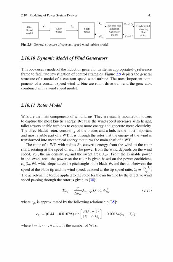
Fig. 2.9 General structure of constant-speed wind turbine model

2.10.10 Dynamic Model of Wind Generators

This book uses amodel of the induction generatorwritten in appropriate d-q referenceframe to facilitate investigation of control strategies. Figure 2.9 depicts the generalstructure of a model of a constant-speed wind turbine. The most important com-ponents of a constant speed wind turbine are rotor, drive train and the generator,combined with a wind speed model.

2.10.11 Rotor Model

WTs are the main components of wind farms. They are usually mounted on towersto capture the most kinetic energy. Because the wind speed increases with height,taller towers enable turbines to capture more energy and generate more electricity.The three bladed rotor, consisting of the blades and a hub, is the most importantand most visible part of a WT. It is through the rotor that the energy of the wind istransformed into mechanical energy that turns the main shaft of a WT.

The rotor of a WT, with radius Ri, converts energy from the wind to the rotorshaft, rotating at the speed of ωmi . The power from the wind depends on the windspeed, Vwi , the air density, ρi, and the swept area, Awti . From the available powerin the swept area, the power on the rotor is given based on the power coefficient,cpi(λi, θi), which depends on the pitch angle of the blade, θi, and the ratio between the

speed of the blade tip and the wind speed, denoted as the tip-speed ratio, λi = ωmi Ri

Vwi.

The aerodynamic torque applied to the rotor for the ith turbine by the effective windspeed passing through the rotor is given as [30]:

Taei = ρi

2ωmi

Awti cpi(λi, θi)V3wi

, (2.23)

where cpi is approximated by the following relationship [35]:

cpi = (0.44 − 0.0167θi) sin

[π(λi − 3)

15 − 0.3θi

]− 0.00184(λi − 3)θi,

where i = 1, · · · , n and n is the number of WTs.


A controller equipped with a WT starts up the machine at wind speeds of about8–16 miles per hour (mph) and shuts it off at about 55 mph. Turbines do not operateat wind speeds above about 55 mph because they might be damaged. The radius ofa 2 MW wind turbine is about 80m, the typical value of air density is 1.225 kg/m3,cp is in the range of 0.52–0.55, towers range from 60 to 90 m (200 to 300 feet) talland the blades rotate at 10–22 revolutions per minute.

Equation 2.23 shows that aerodynamic efficiency is influenced by variation inthe blade’s pitch angle. Regulating the rotor blades provides an effective meansof regulating or limiting the turbine power during high wind speeds or abnormalconditions. A pitch controlled turbine performs power reduction by rotating eachblade about its axis in the direction of the angle of attack. In comparison with thepassive stall, the pitch control provides greater energy capture at the rated wind speedand above. The aerodynamic braking facility of the pitch control can reduce extremeloads on a turbine and also limit its power input so as to control possible over-speedof the machine if the loading of the turbine-generator system is lost, for instance,because of a power system fault. On a pitch-controlled WT, electronic controllerscheck the power output of the turbine several times per second. When the poweroutput becomes too high, a message is sent to the blade-pitch mechanism whichimmediately turns the rotor blades slightly in an attempt to restore this output toan acceptable value. In this work, the pitch-rate limit is set to the typical value of12 deg s−1.

2.10.12 Shaft Model

A two-mass drive train model of a WT generator system (WTGS) is commonly usedas drive train modeling can satisfactorily reproduce the dynamic characteristics ofa WTGS because the low-speed shaft of a WT is relatively soft [36]. Therefore,although, it is essential to incorporate a shaft representation into the constant-speedwind turbine model, only a low-speed shaft is included. The gearbox and high-speed shaft are assumed to be infinitely stiff. The resonance frequencies associatedwith gearboxes and high-speed shafts usually lie outside the frequency bandwidthof interest [37]. Therefore, we use a two-mass representation of the drive train.

The drive train attached to the WT converts the aerodynamic torque, Taei , onthe rotor into the torque on the low-speed shaft, which is scaled down through thegear-box to the torque on the high-speed shaft. The first mass term stands for theblades, hub and low-speed shaft and the second for the high-speed shaft with inertiaconstants, Hmi and HGi , respectively. The shafts are interconnected by a gear ratio,Ngi , combinedwith torsion stiffness,Ksi , and torsion damping,Dmi andDGi , resultingin the torsion angle, γi. The normal grid frequency is f . The dynamics of the shaftare represented as in [30]:

ωmi = 1

2Hmi

[Taei − Ksiγi − Dmiωmi

], (2.24)


ωGi = 1

2HGi

[Ksiγi − Tei − DGiωGi

], (2.25)

γi = 2π f (ωmi − 1

Ngi

ωGi). (2.26)

The generator receives the mechanical power from the gear-box through the stiffshaft. The relationship between the mechanical torque and the torsional angle isgiven by:

Tmi = Ksiγi. (2.27)

The gear-box connects the low-speed shaft to the high-speed shaft and increasesthe rotational speeds from about 30 to 60 rotations per minute (rpm) to about 1,000–1,800 rpm, which is the rotational speed required by most generators to produceelectricity.

2.10.13 Induction Generator Model

An IG can be represented in different ways, depending on the level of detail charac-terised mainly by the number of phenomena, such as stator and rotor flux dynamics,magnetic saturation, skin effects and mechanical dynamics included. Although, avery detailed model which includes all these dynamics is a possibility, it may not bebeneficial for stability studies because it increases the complexity of the model andrequires time-consuming simulations. More importantly, not all of these dynamicsare shown to have significant influence in stability studies.

A comparison of different induction generator models can be found in [30].Accordingly, as the inclusion of iron losses in a model is a complicated task, itsinfluence for stability studies is neglected. The main flux saturation is only of impor-tance when the flux level is higher than the nominal level. Hence, this effect can beneglected for most operating conditions. The skin effect should only be taken intoaccount for a large-slip operating condition which is not the case for a FSWT.

Another constraint of including dynamics in a model is the availability of relevantdata. Typically, saturation and skin effect data are not provided by manufacturers.Therefore, in general, it is impractical to use them in WT applications. For therepresentation of FSIG models in power system stability studies [38], the stator fluxtransients can be neglected in the voltage relations.

All of these arguments lead to the conclusion that rotor dynamics are only themajor factors required to be considered in an IGmodel for a voltage stability analysis.Representation of the third-order model of an IG offers a compatibility with thenetwork model and provides more efficient simulation time. The main drawbacks ofthe third-order model is its inability to predict peak transient current and, to someextent, its less accurate estimation of speed. However, at a relatively high inertia, thethird-order model is sufficiently accurate.


The transient model of a SCIG is described by the following DAEs [30, 34]:

si = 1

2HGi

[Tmi − Tei

], (2.28)

E′qri

= − 1

T ′oi

[E′

qri− (Xi − X ′

i )idsi

]− siωsE

′dri

, (2.29)

E′dri

= − 1

T ′oi

[E′

dri+ (Xi − X ′

i )iqsi

]+ siωsE

′qri

, (2.30)

Vdsi = Rsi idsi − X ′i iqsi + E′

dri, (2.31)

Vqsi = Rsi idsi + X ′i iqsi + E′

qri, (2.32)

vti =√

V2dsi

+ V2qsi

, (2.33)

where X ′i = Xsi + Xmi Xri/(Xmi + Xri) is the transient reactance, Xi = Xsi + Xmi the

rotor open-circuit reactance, T ′oi

= (Lri + Lmi)/Rri the transient open-circuit timeconstant, vti the terminal voltage of the IG, si the slip, E′

drithe direct-axis transient

voltages, E′qri

the quadrature-axis transient voltages, Vdsi the d-axis stator voltage,Vqsi the q-axis stator voltage, Tmi the mechanical torque, Tei = Edri idsi + Eqri iqsi ,the electrical torque, Xsi the stator reactance, Xri is the rotor reactance, Xmi themagnetising reactance, Rsi the stator resistance, Rri the rotor resistance, HGi theinertia constant of the IG, and idsi and iqsi the d- and q-axis components of the statorcurrent, given by:

Idi =n∑

j=1

[E′

drj(Gij cos δji − Bij sin δji) + E′qrj(Gij sin δji + Bij cos δji)

],

(2.34)

Iqi =n∑

j=1

[E′

drj(Gijsinδji + Bijcosδji) + E′qrj(Gijcosδji − Bijsinδji)

].

(2.35)

2.10.14 Modeling of DFIG

The equations that describe a SCIG are identical to those of the DFIG except that therotor is short-circuited. The converter forDFIGs [30] used in this book consists of twoVSCs connected back-to-back. This enables variable-speed operation of the WTs byusing a decoupling control schemewhich controls the active and reactive componentsof the current separately. The modeling of IGs for power-flow and dynamic analysesis discussed in [30, 34].


The DC-link dynamic of a DFIG is given by:

Civdci vdci = − v2dci

Rlossi

− Pri(t) − Pgi(t) (2.36)

where resistor Rlossi represents the total conducting and switching losses of theconverter. Also, Pri(t) is the instantaneous input rotor power, and Pgi(t) is the instan-taneous output power of the GSC which are given by:

Pri = vrdi irdi + vrqi irqi , (2.37)

Pgi = vgdi igdi + vgqi igqi . (2.38)

2.10.15 Aggregated Model of Wind Turbine

The development of aggregated models of wind farms is also an important issuebecause, as the sizes and numbers of turbines on wind farms increase, representingwind farms as individual turbines increases complexity and leads to a time-consumingsimulation which is not beneficial for stability studies of large power systems.

For the aggregation of WTs, the models of several identical WTs (even in theincoming wind) are combined in a single turbine model with a higher rating. Theparameters are obtained by preserving the electrical and mechanical parameters ofeach unit, and by increasing the nominal power to the equivalent of the involvedturbines in the aggregation process [39].

This aggregated model reduces computation and simulation times in comparisonwith those of a detailed model with different representations of tens or hundreds ofturbines and their interconnections. However, the aggregated model requires specificcare in choosing what to aggregate in order to be as close to reality as possible. Inaddition, this type ofmodeling is very difficult forWTswithout a parallel distribution(i.e., in the form of an array which is the most common distribution for offshore, butnot for onshore, wind farms).

2.10.16 Modeling of PV Unit

As shown in Fig. 2.10, PV plants have mainly two parts (a) solar conversion and (b)electrical interface with the electrical network (a power electronic converter). A PVarray is connected to the grid through a DC–DC converter and a DC-AC inverter. ADC–DC converter enables the transfer of maximum power from the solar module tothe inverter. The PV array as shown in Fig. 2.11 is described by its current-voltagecharacteristics function [40, 41]:


Fig. 2.10 Block Diagram of a PV System

Fig. 2.11 Equivalent circuit of a PV array

ipvi= Npi

ILi − NpiIsi

[exp

[αpi

(vpvi

Nsi

+ Rsi ipvi

Npi

)]− 1

]

− Npi

Rshi

(vpvi

Nsi

+ Rsi ipvi

Npi

), (2.39)

where ILi is the light-generated current, Isi is the reverse saturation current, chosenas 9× 10−11A, Nsi is the number of cells in series and Npi is the number of modulesin parallel, Rsi and Rshi are the series and shunt resistances of the array respectively,ipvi is the current flowing through the array, and vpvi is the output voltage of the array.The constant αpi in Eq. (9.1) is given by

αpi = qi

AikiTri(2.40)

where ki = 1.3807×10−23JK−1 is theBoltzmann constant, qi = 1.6022×10−19 C isthe charge of the electron,Ai is the p–n junction ideality factor with a value between 1and 5, and Tri is the cell reference temperature. The schematic of a grid-connected PVsystem consisting of switching elements is shown in Fig. 2.12 [42, 43]. A nonlinearmodel of the three-phase grid connected PV system shown in Fig. 2.12 can be writtenas [42, 43]:

http://dx.doi.org/10.1007/978-981-287-116-9_9


Fig. 2.12 PV system connected to the grid

i1ai = − Ri

L1i

i1ai − 1

L1i

eai + vpvi

3L1i

(2Kai − Kbi − Kci)

i1bi = − Ri

L1i

i1bi − 1

L1i

ebi + vpvi

3L1i

(−Kai + 2Kbi − Kci) (2.41)

i1ci = − Ri

L1i

i1ci − 1

L1i

eci + vpvi

3L1i

(−Kai − Kbi + 2Kci)

vcfai = 1

Cfi

(i1ai−i2ai

), vcfbi = 1

Cfi

(i1bi−i2bi

)vcfci = 1

Cfi

(i1ci − i2ci

), i2ai = 1

L2i

(vcfai − eai

)(2.42)

i2bi = 1

L2i

(vcfbi − ebi

), i2ci = 1

L2i

(vcfci − eci

)

where Kai , Kbi , and Kci are the binary input switching signals. By applying KCL atthe node where the DC link is connected, we get

vpvi= 1

Ci

(ipvi

− idci

). (2.43)

The input current of the inverter idci can be written as [43]

idci = iai Kai + ibi Kbi + ici Kci . (2.44)

Now Eq. (2.43) can be rewritten as:

vpvi= 1

Ciipvi

− 1Ci

(iai Kai + ibi Kbi + ici Kci

). (2.45)


Equations (2.41) and (2.45) can be transformed into dq frame using the angularfrequency ωi of the grid as:

L1i i1di = −Rii1di + ωiL1i i1qi− vcfdi + Kdi vpvi

L1i i1qi= −Rii1qi

− ωiL1i i1di − vcfqi+ Kqi

vpvi

L2i i2di = +ωiL2i i2qi+ vcfdi − Edi

L2i i2qi= −ωL2i2d + vcfq − Eq (2.46)

Cfi vcfdi = ωiCfi vcfqi+ Cfi

(i1di − i2di

)Cfi vcfqi

= −ωiCfi vcfdi + Cfi

(i1qi

− i2qi

)Civpvi

= ipvi− i1di Kdi − i1qi

Kqi

The synchronization scheme for abc → dq transformation is chosen such thatthe q-axis of the dq frame is aligned with the grid voltage vector, Eqi

= 0, and thereal and reactive power delivered to the grid can be written as Pi = 3

2Edi Idi andQi = − 3

2Edi Iqi.

2.10.17 Modeling of FACTS Devices

In general, FACTS devices can be utilised to increase the transmission capacity, thestability margin and dynamic behaviour and serve to ensure improved power quality.Their main capabilities are reactive power compensation, voltage control and power-flow control. Due to their controllable power electronics, FACTS devices alwaysprovide fast controllability in comparison with that of conventional devices, suchas switched compensation or phase shifting transformers. Different control optionsprovide high flexibility and lead to multi-functional devices.

Several kinds of FACTS devices have been developed and there are several yearsof documented evidence of their use in practice and research. Some of them, such asthe thyristor based SVC, are widely applied technology; others, like the VSC-basedSTATCOMs or the VSC high voltage DC (HVDC) are being used in a growingnumber of installations worldwide. The most versatile FACTS devices, such as theunified power-flow controller (UFPC) are still confined primarily to research anddevelopment applications. In this book, we mainly use a STATCOM and, in fewcases, SVC and thyristor-controlled switched capacitors (TCSCs).

2.10.18 STATCOM Model

The concept of the STATCOMwas proposed by Gyugyi in 1976 [44]. A STATCOMis a shunt FACTS device which is mostly employed for controlling the voltage at


Fig. 2.13 Schematic diagram of VSC-based STATCOM

the point of connection to the network, as shown in Fig 2.13. In general, a STAT-COM system consists of three main parts: a VSC; a coupling reactor or a step-uptransformer; and a controller. The magnitude and phase of VSC’s output voltage,Vi, can be regulated through the turn-on/turn-off of the VSC switches so that theVSC output current, I , can be controlled. Here, I is equal to the sum of Vi minus thevoltage at an AC point of common coupling (PCC), Vs, divided by the impedance ofthe coupling reactor, Xs. In other words, the capacitive or inductive output currentsof a STATCOM can be achieved through regulating the magnitude of Vi to be largeror smaller than the magnitude of Vs. Meanwhile, the phase of Vi is almost in phasewith Vs but has a small phase-shift angle to compensate for the converter’s internalloss, thereby keeping the system stable. Therefore, I can be controlled inherentlyand independently of Vs.

By controlling the magnitude and angle of its output voltage, i.e., Vi∠α, theSTATCOM is able to control its active and reactive exchanges with the power systemand, therefore, control the voltage at the PCC.The real and reactive power expressionsare given by:

P = ViVs

Xsin(α − θ),

Q = Vi(Vi − Vs cos(α − θ))

X.

The direction of the reactive power flow can now be determined by the magnitudeof the inverter output voltage. For values of Vi larger than Vs, a STATCOM is inthe capacitive mode and injects reactive power into the network while, for Vi valuessmaller than Vs, it is in the inductive mode and absorbs reactive power from thenetwork. In a typical STATCOM with a capacitor as the DC link, the values of theactive and reactive power depend on one another. However, a STATCOM connected


Fig. 2.14 Schematic diagramof STATCOM

klvdcl∠θl +φl

converter

Rl

Ll

Vl∠θl···

+vdcl − Cl RCl

PLL

θl

+φl

kL

to a battery energy storage system (STATCOM/BESS) is capable of controlling thevalues of both the active and reactive power independently [45].

For the purposes of stability studies, the STATCOM shown in Fig. 2.14 can bemodelled as an AC voltage source with controllable magnitude and phase [46]. Thedynamics of this voltage source are governed by the charging and discharging of alarge (nonideal) capacitor. The capacitor, Cl, and its resistance, RCl , are shown inFig. 2.14. TheDCvoltage across the capacitor is inverted and connected to an externalbus via a short transmission line and a transformer bus. Details of various inverterschemes and how a controllable phase and magnitude are achieved are describedin [44]. The phase-locked loop (PLL) block in Fig. 2.14 indicates that the phase shiftof the inverter wave is adjusted with reference to the external bus voltage.


For the stability analysiswe include the transformer and the transmission line (rep-resented by Rl and Ll in Fig. 2.14) in the reduced impedance matrix. This directlyinterconnects the controllable inverter output with the rest of the system. The capac-itor voltage can be adjusted by controlling the phase-angle difference between theline voltage, Vl, and the VSC voltage, El, (El = klvdcl∠αl). If the phase angle of theline voltage is taken as a reference, the phase angle of the VSC voltage is the sameas the firing angle, αl, of the VSC. Thus, if the firing angles are slightly advanced,the DC voltage, vdcl , decreases and the reactive power flows into the STATCOM.Conversely, if the firing angles are slightly delayed, the DC voltage increases andthe STATCOM supplies reactive power to the bus. By controlling the firing angle ofthe VSC, the reactive power can be generated from, or absorbed, by the STATCOMand, thus, voltage regulation can be achieved.The dynamics for lth STATCOM canbe described by the following equation:

vdcl (t) = − Psl

Clvdcl

− vdcl

RCl Cl, (2.47)

for l = 1, . . . , m where m is the number of STATCOMs, vdcl the capacitor voltage,Cl the DC capacitor, RCl the internal resistance of the capacitor, αl the bus angle ofthe STATCOM in the reduced network, and Psl the power supplied by the system tothe STATCOM to charge the capacitor which is given by:

Psl = |El|2Gll +m∑

p=1p �=l

|El||Ep|[Blp sin αpl + Gpl cosαlp

],

+n∑

j=1j �=l

|El||E′j |

[Blj sin(δj − αl) + Glj cos(δj − αl)

], (2.48)

where Glp and Blp are the real and imaginary parts of the equivalent transferimpedances between the terminal buses of STATCOMs l and p and Glj and Bljare between the terminal buses of STATCOM l and IG j. The term E′

j denotes bothE′

drj and E′qrj and sin αpl = sin(αp − αl).

The terminal voltage of STATCOMs ismeasured using a transducerwith firs-orderdynamic:

vtml = −vtml

Tml

+ Kml vtl , (2.49)

where vtml is the sensor output, vtl the voltage at the connection point of STATCOM,Kml the constant and Tml the time constant of the voltage transducer. For the linearanalysis we can assume that we know the equilibrium condition α0 and control onlyΔα as shown in Fig. 2.15.


klvdcl∠αl

converter

···

+vdcl − Cl RCl

αl+

α0l

Δα l

kl

Fig. 2.15 STATCOM (equivalent)

+

−

|E0i |

KMac

sTMac + 1

|Ei|

controllerk

Fig. 2.16 Modulation index (k) control

The indirect conventional controllers for k and α are shown in Figs. 2.16 and 2.17.This gives an idea of the controller structure used by the industry. In this research,we will control Δk and Δα for the STATCOM in Fig. 2.15 directly instead of usingconventional controllers.


+

−

v0dci

KMac

sTMac + 1

vdci

controllerαi

+

−α0

Δα i

Fig. 2.17 Firing angle (α) control

2.10.19 SVC Modeling

By providing dynamic reactive power, SVC can be used for the purpose of regulat-ing the system voltage, compensating the voltage at a reasonable level, improvingthe power flow capacity of a transmission line, enhancing the damping of low fre-quency oscillations as well as inhibiting the sub-synchronous oscillations. SVC isalso capable of inhibiting the variation of busbar voltage caused by the fluctuatingload, which is favourable for the recovery of transient voltage and the improvementof stabilisation of the system voltage.

For industrial users, it can effectively control the reactive power, improve thepower factor, reduce the voltage influence and harmonic interference caused by thenonlinear load, balance the three-phase load, improve the power quality, productiveefficiency and the product quality, and reduce the energy consumption. It is widelyused in the machine, electric power, metallurgy, electrified railway, mine and windpower generation industries. The overall performance indicators are given below:

• SVC dynamic capacity: 0–400 MVAr;• control-target bus rated voltage: 6–500 kV;• total dynamic response time: (reactive power output): <15 ms; and• SVC biggest loss: <0.8%.

The SVC circuit contains the voltage measuring and voltage regulator circuits,outputs of which are fed into the thyristor firing control circuit. Normally, the sus-ceptance of the SVC (B) is varied to maintain the mid-bus voltage, Vm, within itspre-specified tolerance. The supplementary stabilising signal is added to the outputof the voltage regulator. The variation of the susceptance (B) can be related throughthe differential equation:

�Bl = [−�Bl + Bl0 + Kcl Vsl

]/Tcl , (2.50)


Fig. 2.18 One-line diagram of single-phase TCSC

for l = 1, . . . , m, where m is the number of SVC, Kcl and Tcl the gain and timeconstants of the SVC’s firing angle control circuit, respectively, and Vsl the extrastabilising signal.

2.10.20 Thyristor Controlled Series Capacitor

After the introduction of TCSC in the late 1980s, they have been implemented inseveral locations around the world. As a controllable series compensation deviceand with flexible control possibilities, the TCSC has been found to be effective,especially in damping electromechanical and sub-synchronous oscillations. With aproperly designed control system, a TCSC can be effectively utilised for enhancingboth small signal and transient stabilities of a power system. Therefore, a goodunderstanding of the interaction phenomena between a TCSC and its surroundingnetwork will be necessary in order to design optimal control structures and, at thesame time, prevent undesired interactions.

The single-line diagram of a TCSC is shown in Fig. 2.18. The operation of a TCSCinvolves discrete actions and is periodic in nature, whereby one of its anti-parallelthyristors of the TCSC is turned on during a portion of a half-cycle of the powerfrequency and is turned-off during the remainder of the cycle. The other anti-parallelthyristor repeats the conduction/non-conduction process during the next half cycleand vice versa. The duration and timing of thyristor conductions are based on thetriggering logic and are controlled by the synchronisation system and the higher-level control loops. When a thyristor conducts, a circulating current flows in both theinductor and the capacitor which can either increase or decrease the voltage acrossthe capacitor.

2.10.21 Energy Storage Device

The energy storage system (ESS), as an enabling infrastructure technology, pro-vides ride-through over outages, improves profitability in high-energy applications,


increases system reliability and dynamic stability, improves power quality andenhances transmission capacity of the transmission grid in a high power applica-tion [44]. For a high power application, the use of short-term (cycles to seconds)energy storage integrated with a power electronics-based controller, well known asa FACTS controller, could offer the following three distinct advantages:

• provide system damping, while maintaining constant voltage following a distur-bance;

• provide additional damping in situations where the dynamic reactive power pro-vided by traditional FACTS controllers with similar ratings is inadequate (alter-natively, it could provide the same amount of damping at less cost. The dampingof oscillation, by repeatedly interchanging small amounts of real power with thesystem, would be an excellent ESS application); and

• provide energy to maintain the speed of locally connected induction motors duringa power system disturbance (This may prevent a voltage collapse in areas wherethere is a large concentration of induction motors that would otherwise stall).

While the superconductive magnetic energy storage (SMES) technology over-comes many barriers from a technology perspective, and has been commerciallyavailable in some specific sizes, the cost and relative complexity of the overall SMESsystem still makes it an expensive choice for a short-term ESS [47].

Recent advances in supercapacitor (SCAP) technology with an asymmetricaldesign have brought much excitement to the industry with the hope of a new andbetter short-term energy storage solution [48]. SCAP, as one type of electrochemi-cal capacitor, stores electrical energy in the electrical double layer using relativelyinexpensive materials, provides energy density thousands of times larger than thatof conventional electrolytic capacitors, and has miscellaneous advantages over otherhigh-power energy storage devices: high power density, low cost, reliable and longlife cycle, fast and deep charge/discharge capability, wide range of operational tem-peratures, maintenance-free operation and storage, and environmental safety. Thesecharacteristics make SCAP a desirable energy storage element for short-term high-power ESS applications [49].

2.10.22 Network Power-Flow Model

The power balance equations pertaining to generator buses are given by:

Vi cos(δi − θi)Iqi − Vi sin(δi − θi)Idi − Spi = 0, (2.51)

−Vi sin(δi − θi)Iqi − Vi cos(δi − θi)Idi − Sqi = 0, (2.52)


where,

Spi =n∑

k=1

ViVk [Gik cos(θi − θk) + Bik sin(θi − θk)] , (2.53)

Sqi =n∑

k=1

ViVk [Gik sin(θi − θk) − Bik cos(θi − θk)] , (2.54)

for i = 1, 2, . . . , m.The power balance equations for non-generator buses are given by:

PLi(Vi) +n∑

k=1

ViVk [Gik cos(θi − θk) + Bik sin(θi − θk)] = 0, (2.55)

QLi(Vi) +n∑

k=1

ViVk [Gik sin(θi − θk) − Bik cos(θi − θk)] = 0, (2.56)

for i = m + 1, m + 2, . . . , n, where , n is the total number of buses in the systemand Yik = Gik + jBik the element of the ith row and kth column of the bus admittancematrix Y .

2.10.23 Power System Modeling

Power system modeling requires the modeling of all system components including,generators, transmission lines, transformers, loads and other control devices/systems,as discussed above. A complete power system modeling approach involves formingthe overall system equations in the form of DAEs as:

x = f (x, z, p), (2.57)

0 = g(x, z, p), (2.58)

where x is the vector of state variables, z the vector of algebraic variables and p thevector of system parameters. The differential equation set includes the dynamics ofgenerators, excitation systems, load dynamics, and the algebraic equation set includesload flow equations and other algebraic relationship among the system components.

In power system modeling studies, the parameter values are chosen as eitherfixed values or within a certain range because the measurement of actual systemparameters is very difficult. In particular, the load parameter values are difficult toobtain due to the large number of load components, the inaccessibility of certaincustomer loads, load compensation variations and the uncertainties of many loadcomponent characteristics.

2.11 Chapter Summary 57

2.11 Chapter Summary

The basic ideas about voltage instability and the importance of voltage instabilityanalysis are explained from a fundamental as well as practical point of view in thischapter. The main focus of the chapter is to provide underlying causes of voltageinstability, and the identification of different categories of stability behaviours thatare important in power system stability analysis. The methods of improving voltagestability are also outlined.

In addition, this chapter discusses the dynamic modeling of a large power system.To provide a reliable model for implementation in a standard simulation tool, severalfactors must be taken into account. The first important process is to clearly define thepurpose of the study. Each type of power system study requires a particular frequencybandwidth and a simulation time-frame depending on how fast the system dynamicsneeds to be investigated. Subsequently, the nature of the system being modelled mustbe carefully understood and the simulation tool used to simulate the models must beappropriately utilised.

Linear feedback control in power systems has a long history in terms of researchand application. Linear controllers are preferred over nonlinear controllers becausethey impose lower requirements on practical implementation. However, as powersystem components are nonlinear in order to design a linear controller, linear modelsof a nonlinear system are needed. Different linearisation and modal analysis tech-niques will be discussed in the next chapter.

References

1. Vassell GS (1991) Northeast blackout of 1965. IEEE Power Eng Rev 11(1): 4–82. LuW, Besanger Y, Zamai E, Radu D (2006) Blackouts: description, analysis and classification.

In: 6th WSEAS international conference on power systems, pp 429–4343. Custem TV, Vournas CD (1998) Voltage stability of the electric power systems. Kluwer Aca-

demic, Norwell4. Berizzi A (2004) The Italian 2003 blackout. In: IEEE power engineering society general meet-

ing, Denver, CO, pp 1673–16795. Ohno T, Imai S (2006) The 1987 Tokyo blackout. In: IEEE PES power systems conference and

exposition, Atlanta, GA, pp 314–3186. Andersson G, Donalek P, Farmer R, Hatziargyriou N, Kamwa I, Kundur P (2005) Causes of

the 2003 major grids blackouts in North America and Europe, and recommendationed meansto improve system dynamic performance. IEEE Trans Power Syst 20(4): 1922–1928

7. U.S. Canada Power SystemOutage Task Force (2004) Final report on theAug 14 2003 blackoutin the United States and Canada: causes and recommendations

8. Gao B, Morison GK, Kundur P (1996) Towards the development of a systematic approachfor voltage stability assessment of large-scale power systems. IEEE Trans Power Sys 11(3):1314–1324

9. Hossain MJ, Pota HR, Ugrinovski V (2008) Short and long-term dynamic voltage instability.In: 17th IFAC World Congress, Seoul, Korea, pp 9392–9397

10. IEEE (1990) Special publication 90TH0358-2-PWR: voltage stability of power systems: con-cepts, analytical tools, and industry experience


11. Vournas CD, Sauer PW, Pai MA (1996) Relationships between voltage and angle stability ofpower systems. Int J Electr Power Energy Syst 18(8): 493–500

12. Chi Y, Liu Y, Wang W, Dai H (2006) Voltage stability analysis of wind farm integration intotransmission network. In: International conference on power system technology, pp 1–7

13. Lei Y, Mullane A, Lightbody G, Yacamini R (2006) Modeling of the wind turbine with adoubly-fed induction generator for grid integration studies. IEEE Trans Energy Convers 21(1):257–264

14. Morison GK Gao B, Kundur P (1993) Voltage stability analysis using static and dynamicapproaches. IEEE Trans Power Syst 8(3): 1159–1171

15. Taylor CW (1994) Power system voltage stability. McGraw-Hill, New York16. Cutsem TV, Vournas C (1998) Voltage stability of electrical power system. Kluwer Academic,

Norwell17. Cutsem TV (2000) Voltage instability: phenomenon, countermeasures and analysis methods.

Proc IEEE 88(2): 208–22718. Kundur P (1994) Power system stability and control. Mcgraw-Hill, New York19. Cutsem TV, Mailhot R (1997) Validation of a fast voltage stability analysis method on the

Hydro-Quebec system. IEEE Trans Power Syst 12(1): 282–29220. Ainsworth JD, Gavrilovic A, Thanawala HL (1980) Static and synchronous compensators for

HVDC transmission convertors connected to weak AC systems. In: 28th session CIGRE, pp31–41

21. Molinas M, Suul JA, Undeland T (2008) Low voltage ride through of wind farms with cagegenerators: STATCOM versus SVC. IEEE Trans Power Electr 23(3): 1104–1117

22. Molinas M, Suul JA, Undeland T (2006) Wind farms with increased transient stability marginprovided by a STATCOM. In: IEEE 5th international conference on power electronics andmotion control, pp 1–7

23. Pal B, Chaudhuri B (2005) Robust control in power systems. Springer, USA24. Bergen AR (1986) Power system analysis. Prentice-Hall, New Jersey25. Das JC, Casey J (1999) Effects of excitation controls on operation of synchronous motors. In:

IEEE industrial and commercial power systems technical conference, Sparks, NV, pp 1–526. Klein M, Rogers GJ, Kundur P (1991) A fundamental study of inter-area oscillations in power

systems. IEEE Trans Power Syst 6(3): 914–92127. IEEE Committee Report (1981) Excitation system models for power system stability studies.

IEEE Trans Power Apparatus Syst PAS 100(2): 494–50928. Rogers G (2000) Power system oscillations. Kluwer Academic Publishers, Boston29. Hill DJ (1993) Nonlinear dynamic load models with recovery for voltage stability studies.

IEEE Trans Power Syst 8(1): 166–17630. Ackermann T (2005) Wind power in power systems. Wiley, England31. Li H, Chen Z (2008) Overview of different wind generator systems and their comparisons. IET

Renew Power Gener 2(2):123–13832. Morren J, de Haan SWH (2005) Ride-through of wind turbines with doubly-fed induction

generator during a voltage dip. IEEE Trans Energy Convers 20(2): 435–44133. Permitting of Wind Energy Facilities (2002) A handbook prepared by National Wind Coordi-

nating Committee (NWCC) Siting Subcommittee, Aug 200234. Nandigam K, Chowdhury BH (2004) Power flow and stability models for induction generators

used in wind turbines. In: IEEE power engineering society general meeting, Denver, CO, pp2012–2016

35. Abdin ES, Xu W (2000) Control design and dynamic performance analysis of a wind turbine-induction generator unit. IEEE Trans Energy Convers 15(1): 91–96

36. Akhmatov V, Knudsen H (2002) An aggregate model of a grid-connected, large-scale, offshorewind farm for power stability investigations-importance of windmill mechanical system. Int JElectr Power Energy Syst 24(9): 709–717

37. Akhmatov V, Knudsen H, Nielsen A (2000) Advanced simulation of windmills in the electricalpower supply. Int J Electr Power Energy Syst 22(6): 421–434

References 59

38. Feijo A, Cidrs J, Carrillo C (200) A third order model for the doubly-fed induction machine.Electric Power Syst Res 56(2): 121–127

39. Ledesma P, Usaola J, Rodriguez JL (2003) Transient stability of a fixed speed wind farm.Renew Energy 28(9): 1341–1355

40. Mahmud MA, Pota HR, Hossain MJ (201)2 Dynamic stability of three-phase grid-connectedphotovoltaic system using zero dynamic design approach. IEEE J Photovoltaics 12(4): 564–571

41. Mahmud MA, Pota HR, Hossain MJ (2011) Modeling guidelines and a benchmark for powersystem simulation studies of three-phase single-stage photovoltaic systems. IEEE Trans PowerDeliv 26(2): 1247–1264

42. TanYT,KirschenDS, JenkinsN (2004)Amodel of PVgeneration suitable for stability analysis.IEEE Trans Energy Convers 19: 748–755

43. Nosrat A, Pearce, J.M.: Dispatch strategy and model for hybrid photovoltaic and tri-generationpower systems. Appl Energy 88(9): 3270–3276

44. Hingorani MG, Gyugyi L (2000) Understanding FACTS: concepts and technology of flexibleAC transmission systems. IEEE Press, New York

45. Divya KC, Ostergaard J (2009) Battery energy storage technology for power systems—anoverview. Electric Power Syst Res 79(4): 511–520

46. Acha E, Fuerte-Esquivel CR, Ambriz-Perez H, Angles-Camacho C (2004) FACTS modelingand simulation in power networks. Wiley, London

47. Karasik V, Dixon K, Weber C, Batchelder B, Campbell G, Rebeiro P (1999) SMES for powerutility applications: a review of technical and cost considerations. IEEE Trans Appl Supercond9(2): 541–546

48. Lasseter RH, Jalali SG (1991) Power conditioning systems for superconductive magneticenergy storage. IEEE Trans Energy Convers 6(3): 381–387

49. Varakin IN, KlementovAD, Litvinenko SV, StarodubtsevNF, StepanovAB (1997) Applicationof ultracapacitors as traction energy sources. In: Proceedings of 7th international seminar ondouble layer capacitors and similar energy storage devices, Florida, USA

http://www.springer.com/978-981-287-115-2

Power System Voltage Stability and Models of Devices

Documents

Transcript of Power System Voltage Stability and Models of Devices