1

Power Metering Fundamentals Jim Spangler Cirrus Logic

1 March 2011

Abstract: This paper defines how to measure electrical energy using electronic wattmeters, for both single phase and multiphase applications for Power Monitoring while Utility grade measurement for revenue is left for others. Historical and current electronic measurement connections are shown. Included are multiphase transformer characteristics that to go from Wye to Delta and Delta to Wye configurations. Several multiphase electrical power measurement techniques using a three wattmeter approach will be compared to a two wattmeter approach along with some inaccuracies. A three wattmeter approach is presented as an accurate method for both balanced and unbalanced multiphase load conditions. The next section discusses the third order harmonic cancellations that occur when transferring between a Delta to Wye or from a Wye to Delta transformer for utility power transmissions. The final section describes using the CRD5463PM to obtain additional data like THD. Watt Meters Wattmeters are instruments that measure the true wattage used or delivered to a load. These instruments have two separate inputs: voltage current. In analog instruments these inputs are coils: there is the voltage coil and there is a current coil. In today’s electronic wattmeter’s the coils are replaced with resistors. The current through these resistors creates a voltage that can be measured by an analog to digital converter (ADC.) The ADC produces a digital representation of the voltage and current. This digital representation of the voltage and current can be multiplied together digitally to obtain true power per sample of time. Other items used in utility grade meters include: Apparent Power (S), Reactive Power (VAR), and Kilowatt-Hours metering, that will not be discussed.

The single phase connection is shown in Figure 1 below. The current measurement is shown as A while the voltage measurement is shown as V. The connection is identical for an analog and digital wattmeter. The electronic version of Figure 1 is shown in Figure 2 which uses a Cirrus Logic CS5463 that would interface with a microprocessor or use or drive analog meters with the energy output ports. This is described in the CS5463 data sheet, or is available on www.cirrus.com.

Figure 1. Simple Wattmeter connection between source and load In Figure 2, the voltage across the shunt resistor (Rshunt) represents the current flowing through the power lines. The voltage developed across R1 represents the voltage delivered to the load. The CS5463 samples this voltage using a signed 24 bit Sigma-Delta (Σ−Δ) technique (23 bit data 1 bit

2

sign) then multiples the two together to obtain a 24-bit (signed) representation of the power or energy used between sample times, which is every 125 micro-seconds (uSec) when a 4.049 MHz crystal is used.

Figure 2. The CS5463 in a typical application that uses a current shunt, RShunt, for the current input and R1 for the voltage. As an example, when the Source, shown in Fig. 1, is a 12Vac and the load is resistive similar to a a heater or incandescent lamp of 6 ohms, 2 Amps or 24 Watts are dissipated or used. The graph is shown in Fig. 3. The values where chosen to provide simple scaling; notice the wattage goes only positive despite the voltage and current both go negative. (Remember algebra negative multiplied by a negative is a positive). This excel graph was created, in the same way the CS546x, CS548x and CS549x family of products operate. There is a sampling of the voltage and the current every five (5o) degrees. Please note the purple line showing the average of the wattage that would be read by a calibrated wattmeter. Appendix A has the data for one ac line cycle using 10o increments. The same voltage and current is plotted in Figure 4 but with a 30o degree phase lag of current that would be caused by an inductive and resistive load. Note the instantaneous wattage goes below 0. The total average wattage is now 20.78 watts verses 24 watts as in the pure resistive load condition. The instantaneous wattage for both Figures 3 and 4 is plotted as the “green.” Calculating the average wattage is shown in Equation 1. The instantaneous data is summed at 4000 times a second. The total is divided by 4000 to produce an average over one second. This equation and method works for all types of waveforms including those that contain harmonics. This math is utilized in all the Cirrus Logic Power Metering products.

3

i

N

iiN IVWatts ∑

=

=1

1 Equation 1

iV = Instantaneous voltage at time i iI = Instantaneous current at time i CS546x family makes 4000 samples per second with a 4.049 MHz crystal.

Figure 3. Resistive Load Voltage, Current, and Wattage

Figure 4. Lagging Current effect on Wattage

4

Three Phase Power Most of the utility power generated and transmitted is multi-phase or three phase. Three phases are used because they provide a constant load to the generator and uses the fewest number of transmission lines. Three-phase systems are not the only ones, there could be a four, or five or even higher phase systems. These higher order systems require additional current carrying lines. Figure 5 shows a plot of instantaneous energy in a three phase power system. It is assumed to have perfect power factor where there is no leading or lagging current. Each phase has the same electrical load. When the individual phase powers are added together the effective power is 1.5 times the peak of any individual phase. Where the graph assumes a 1.0 Vac peak voltage and a 1.0 Aac peak current. There is no ripple in the total power sum which indicates the mechanical load to the generator is constant.

Figure 5: Three individual phases of wattage summed together. The sum is 1.5 watts and it is a constant with no ripple.

The same can be done with four phases; see Figure 6. The four individual phases are 90o from each other. But when the voltage and current are multiplied together, the phases that are shown are 180o out of phase with each other, and are aligned on top of each other. Figure 7 shows the four voltages or current phases while Figure 6 shows the phase powers. Only Phase C and Phase D show up because Phase A and Phase B are beneath Phase C and Phase D curves. This additive effect shows the sum of the four individual phases to be twice that of a single phase. Five phases are attempted; this can be seen in Figure 8. It is unknown if there is five phase power system. If one existed, the sum would be 2.5 times the amplitude of any individual phase

An effective six phase system is used in some industrial motor drives. This is accomplished by supplying both a Delta and Wye configuration to a set of twelve rectifiers to produce a dc voltage to high power variable speed motor drives.

5

Figure 6: Four phase power wattage chart. Note the Wattages add up to twice the individual peak power. For two phases to operate they must be 90o out of phase producing a total power equal to the peak of the instantaneous wattage.

Figure 7: Normalized Four Phase Voltages make up the instantaneous power shown in Figure 6. The wattage is effectively the square of the above voltages which causes the values to be positive and two of the phases to be identical.

6

Figure 8: Figure of five phase power. Electrical Power Transmission and Distribution. Today most electrical power is generated and distributed using three phases each spaced 120o from each other. This presents a constant mechanical load to the generation system and allows power to be transmitted using only three wires (Δ or Delta ). Electrical power generation or generators are usually connected in a Wye (Y) configuration and use a step-up transformer (Y-Δ) to convert the generationed power to high voltage. The high voltage provides a lower resistive power loss in the transmission wire due to the lower current. This is often refered to as I squared R loss (I2R). The generator usually does not produce a pure fundamental sine wave. The generated voltage waveform has third order and higher order harmonics. The third order harmonic along with the ninth, fifteenth, etc. cancle out in the Delta to Wye (Δ-Y) or Wye to Delta (Y-Δ) transfomer secondary. The harmonics are still present in the side they are generated primary or secondary but are not transmitted to the other side secondary or primary. Greater discussions are given later sections. Figure 9 shows an electrical generation and transmission system. Electrical Power is created in generation plants by heating water to steam using coal, oil, and natural gas. Steam pressure is regulated to drive the turbines that drive the electrical generators at a constant speed. Electical power generation can also be accomplished by using water pressure to drive turbines at dams (such as the Hoover Dam) and by diverting river water around falls, Niagara Falls, on the Niagara River that connects Lake Eire to Lake Ontario. Hydro-Electric Power Generation is more efficient because no energy is used to heat the water. The generating voltage is between 15 KVac and 30 KVac which is stepped using high voltage step-up transformers usually Wye to Delta (Y-Δ) . The electrical energy is transmitted over the powerline that is between 138 KVac and 765 KVac; see the transmission line system in Figure 9. Near the location where the electrical energy is used, the voltage is stepped down at a distribution point. The distribution system voltage can be as low as 4 KVac and as high as 69 KVac. At the end of the distribution where consumption occurs, the voltage is reduced.

7

The consumption voltage varies but most building and manufacturing companies use “Low Voltage.” The term low voltage refers to anything below 600 Vac. This includes the 208 Vac (Y-3Φ), 240 Vac (Δ-3Φ), 381 Vac (Europe 50Hz, Y-3Φ), 480 Vac (Y-3Φ) and 600 Vac (Y-3Φ) single phase (1θ) three phase systems (3θ). Another term, “Medium Voltage” which referes to 2130 Vac and 4160 Vac that is used for large industrial motor systems like a 1000 horsepower, 1 megawatt motor, or higher power motor systems.

Figure 9. Electrical Power Distribution including generation, transmission, distribution and users.

Three Phase Transformer Connections A three phase isolation transfomrer is shown in Figure 10. All three phases are wound on a single core with each phase on its own leg. Depending upon the turns-ration, the secondary voltage can be higher or lower than the primary voltage. The symbol for a transfomer is shown in Figure 11 with the Delta or Wye symbols shown below the windings. The two types of connections of the three windings are shown in Figure 12. In a Wye (Y) configuration usually 4 wires, the center point is the neutral, (labled as N in Figure 12,) and the sum of the instantaneous of the three voltages add up to zero (0 Vac). The same is true with the neutral, the sum of the instantaneous currents sum up to zero (0 Aac) when there is a balanced system. Effectively the neutral, carries no current and has no voltage, thus has a perfect null (0) point.

8

AP’

AP”AS’

AS”

BP’

BP”BS’

BS” CS”

CS’CP”

CP’Primary Side

Secondary Side

Figure 10. Three Phase Transformer, with each phase on a separate leg, Phase A outer left, Phase B center, and Phase C outer right.

Figure 11. Delta-Wye (ΔY), Delta-Delta (ΔΔ), Wye-Wye(YY), and Wye-Delta(ΔY) connections Figure 12 shows the windings connected using a transformer core shown in Figure 10. The primary could be a Delta, (Δ-3Φ), 13.2 KVac, line-to-line voltage, the secondary could be a four wire Wye 480 (Y-3Φ) Vac line-line industrial voltage. Instead of a 480 Vac, the voltage could be a four wire Wye, (Y-3Φ), 208 Vac line-line voltage for commercial and light industrial applications.

A

BC

Ia

Ib

Ic

VC VB

VA

As’

Bs’Cs’

Ia

Ib

Ic

VAN

VBN

VCN

N

VAB

VA

VBVC

VBC

VCA

V C V A

V B

LNLL VV *3=

ITRANSMISSION LINE

240120 jc

jbTRAN eIeII −=

ccbTRAN IjIII23

21

++=

Equations

loadb II =

Figure 12. Delta (Δ) to Wye (Y) configuration indicated as a (ΔY) or (Δ-Y) transformer. The A and As’ coils, the B and Bs’ coils, and C and Cs’coils are linked magnetically. They are shown in Figure 9 wound on the same leg of the double E core.

9

Three Phase Wattage Measurements. Four Wire Wye There are a number of methods to make three phase wattage measurements. The method used depends upon the configuration: Wye, Delta, or Tapped Delta, of the electrical power delivered to the facility. The easiest to explain is for a “Wye” configuration. A Wye (Y) configuration uses a four wire system consisting of: Phase A, Phase B, Phase C, and a Neutral. In most distribution systems the Neutral is connected to earth ground only at the distribution panel or service panel as shown in Figure 13. This approach uses three wattmeters, one for each of the phases, see Figure 13.

The total wattage used is the sum of the individual phase wattages. This four wire approach, with the neutral, works with both balanced and unbalance loads. A balance load for three phase systems is when the individual phase loads are of the same magnitude value of current in rms and voltage in rms. An unbalanced load is when, the loads are not equal, in most cases the phase load currents do not have the same rms magnitude but the magnitude of the phase voltages are the same. The utility would like to have all the lines carry the same amount or magnitude of current. The utility industry refers to this condition as a unbalanced load when the currents in each are not equal.

Three phase motor loads produce a balanced load. Fluorescent lighting loads and office machines create unequal current draw and also an unbalanced system. The 120 Vac three-socket-outlets in offices are taken from one of the phases. Other phases are used for lighting as is the fluorescent lighting branch circuits. It is almost impossible to balance the other phases so an unbalanced load always exist. The value of this unbalance load is important in order to measure the wattage draw of a three phase load.

A

V

Wattmeter

A

V

Wattmeter

+ +

-

-

++

-

-

A

V

Wattmeter+

+-

-

Neutral

Phase B

Phase C

Phase A

Load B

Load C

Load A

Wye Three Phase Distribution Transformer

ServicePanel

EarthGround

As’

Bs’Cs’

Ia

Ib

Ic

VAN

VBN

VC

N

N

VAB

VA

VBVC

VBC

VCA

WB

WC

WA

Figure 13. Three Phase Load with three wattmeters, WA, WB, and WC. This approach provides the most accurate wattage measurement and is the bases for comparison.

Dual Wattmeter for a Delta or Wye Configuration: a Balanced Load. The most common method of measuring three phase power is with two wattmeters. This is how most balanced load measurements are taken. Previously in the Engineering Lab, one would use a Weston Polyphase Wattmeter Model 329, to measure the wattage for each motor for the total load wattage or two Simpson Dynamometer Panel Meters. One of the phases is used as

10

a reference, as shown in Figure 14. The diagram in Figure 14 shows a balanced load consisting of two induction motors, one a Delta winding type the other a Wye winding type. The reference for the wattmeters is Phase B. The phase is labeled Phase ΔB. The wattmeters are floating on high voltage. Care must be taken since there is a potential electric shock hazard when touching the wattmeter connections. The only earth ground or neutral connection is the chassis of the motor housing and motor shafts. Three phase induction motors are considered balanced loads.

A

BC

Ia

Ib

Ic

VCVB

VA

A

V

Wattmeter+

+-

-

A

V

Wattmeter+

+-

-

Wye Connected

Motor Delta Connected

Motor

Induction Motors

Reference for Watt Meters

No Neutral or Ground Reference

Chassis or Motor Frame is grounded as is the motor shaft

Watt meter are floating on high voltage

Earth Ground

V A

V B

V C

V B

WA

WC

Figure 14. Delta configuration with two wattmeters and a balanced load. There is no neutral connection therefore the voltages are all high with respect to earth ground. This connection is an electrical shock hazard. Electrical motors produce a balanced load. A three phase Wye (Y) electrical input uses the same connection of wattmeters as Delta (Δ) distribution configuration; this is shown in Figure 15. In both Figures 14 and 15, the reference is one of the phases. In Figure 14, the reference was Phase ΔB. In Figure 15 the reference is Phase A. In both systems, the loads are induction motors which provide a balanced load to the electrical system. In Figure 15, a neutral or earth ground is shown how it would be connected and utilized. Induction motors usually have their chassis or frames earth grounded for safety reasons. This earth ground is shown and also connected to the neutral of the system.

11

Figure 15. Two Wattmeter Wye (Y) with Balanced Loads. The neutral is not connected and carries no current. Proof of Delta and Wye Connections Are Accurate

When the instantaneous wattages of each meter is generated and plotted using excel, the results are shown Figure 16. The legend in Figure16 indicates the power for the Delta configuration as connected in Figure 14, with Phase ΔB used as the reference. The power is calculated by multiplying the instantaneous voltage, with its phase angle, multiplied by the instantaneous current coming out of each phase. The two phase powers are summed and they produce the constant load line as indicated by the Sum or the Total Watts in Figure 16, which is a flat green line. In Figure 16 which is normalized to 1.0, the total wattage is 1.5 Watts. The results are identical for a Delta connection. In both cases, Figure 14 and Figure 15, the neutral line carries no current in this balanced system. In fact, a neutral line does not have to be connected, but an earth ground line is always used and is connected to the motor frame for safety.

In Figure 13, there are three loads that be represented as an induction motor(s), the same amount of power is drawn. Figure 5, also shown as Figure 18 below, is identical. This means that the wattmeter connection in Figure 13 could be used in place of wattmeter configuration in Figure 15.

Therefore, in a balanced load, Figures 13, 14, and 15 all produce the same results. This is important because a neutral is not always available so the use of a two wattmeter system is accurate for a balance load condition to report the energy used in watts or watt-hours. The cost of an extra wattmeter is not needed.

12

Figure 16. Wattage for each meter and the sum of the two meters is constant for a balance load. Instead of using two wattmeters, a single wattmeter chip with a microprocessor can be used. The Cirrus Logic, CS5467, and the connection is shown below in Figure 17. The L1 and L2 would be the phase lines Phase A and Phase C while the N would be Phase B. Phase B would be the reference. This would be the practical implimentation of Figure 14 and Figure 15. In practive, there would be several changes in the schematic concering the value of the 2 uF capacitor. The value of this capacitor will change to approximately 1.0 uF for a 120 Vac systems but would be between 0.47 uF and 0.68 uF for a 208 3Φ phase system using 60 Hz.

13

Figure 17. CS5467 performing the two wattmeter system in a single IC. This is a valid connection for three phase Delta or Wye configurations. It is also valid for a split phase connection used in US and Canada split phase 120-240 Vac single phase measurements.

The wattage sum shown in Figure 16 is identical to that presented in Figure 5 and again below as Figure 18. The math sum of the three wattmeters in a three wattmeter system in a “Wye” configuration using a neutral as a reference produces the same results as the two wattmeters added together in dual wattmeter system in balanced load conditions. This means that Figure 13, Figure 14, Figure 15 and the practical example from Figure 17 produce the identical results in both math and metering systems. This is only valid for a balanced three phase system and not a unbalanced system. Unbalanced loads are discussed in the next section.

14

Figure 18. Identialal to Figure 5: Three individual phases of wattage summed together. The results of the three wattmeters are identical to the two wattmeter approach shown in Figure 14 and Figure 15. Unbalanced Loads The information presented has been about balance loads; now the discussion will be about unbalanced loads. The first part is to make Phase A = 1 Aac, Phase B = 1.5 Aac, and Phase C = 2 Aac. The voltage will be at 1 Vac for all three phases. Two complete voltage and current cycles were created in excel, and are shown in Figure 18 below. This is a very busy graph with five curves indicating because the voltage and current curves for Phase A are identical. In this example of a Wye (Y) system the voltage line to neutral voltage is equal to 1Vac while the line currents are 1.0 Aac peak for Phase A (Ia), 1.5 Aac peak for Phase B (Ib) and 2.0 Aac peak for Phase C (Ic). Please note that Va and Ia are identical Ia shows up; one line overlays the other. The equipment setup would be the same as shown in Figure 13 and the voltages are the same, the load currents are different. The load A current is 1 Aac, load B current is 1.5 Aac and load C current is 2.0 Aac. The power for each of these loads and their sum is shown in Figure 19. The Average Power is calculated to be 2.25 watts, which was created by using an excel spreadsheet and performing a calculation every five degrees. (Appendix C data developed every 15 degrees.) The instantaneous wattages were summed and then divided by 72 (which is the total number of measurements made of a complete ac line cycle.) This method is described in Equation 1. The true wattage is now shown and calculated using each phase and summing the total. The instanteous wattage has a high of 2.683 Watts and a low of 1.817 Watts normalized to 1.0 Watts which is Va*Ia. When this unbalanced configuration is plotted, the results are given in Figure 20. Figure 20 shows the instantaneous sum as a “Sum” which is really a constant with a sine wave added. The individual phase wattages are also shown and are labeled Load A, Load B, and Load C which represent the phase loads.

15

Figure 19. Unbalance Currents with Constant Voltage. Wye system shown with the voltage line to neutral equal to 1Vac while the line currents are 1.0 Aac peak for Phase A (Ia), 1.5 Aac peak for Phase B (Ib) and 2.0 Aac peak for Phase C (Ic). Va and Ia are identical and only Ia shown.

Figure 20. Wattage for a 4 Wire Wye Network. Wattage for Phase A is1.0 Watts peak, Phase B is 1.5 Watts peak, and Phase C is 2.0 Watts peak. The effective average is 2.25 Watts.

16

Two Wattmeter Approach, unbalanced load, Phase C as a Reference A two wattmeter approach is used as shown in Figures 14 and 15. The first case is to use Phase C as the reference. In this example, the wattage is shown in Figure 21, the average wattage sum is calculated to be 1.875 watts versus the 2.25 watts using the approach shown in Figure 13, which produces 2.25 watt of normalized power, Phase C, has the highest current. In this extreme example, the wattage is 83.33% of the true wattage or 16.667 lower than what is accurate. Two Wattmeter Approach, Unbalanced Load, Phase A as a Reference In the next example, the reference is changed to Phase A, the wattage per meter and sum is shown in Figure 22. Using Phase A as the references produces an average wattage of 2.625 normalized watts. This is different than using Phase C where the average is 1.875 watts normalized. The 2.625 is 116.667% higher than the true wattage of 2.25 watts.

Figure 21. Unbalance Load with Phase C used as a reference. The average is calculated to be 1.875 watts over a single cycle. The normalized value is 1.0 watt, which is Va*Ia. The true normalized wattage is 2.25 Watts. Two Wattmeter approach, unbalanced, using Phase B as a Reference Using a two wattmeter approach and using Phase B as the reference, this unbalanced system produces, the wattage shown in Figure 23 below. In this case, the average is 2.25 watts. This is same as the 2.25 watts that is shown in Figure 20 which is the standard. In this example, the average is identical as one of the legs. This is not always the case. How can someone determine the proper configuration for obtaining power properly?

17

Figure 22. Two watt meter method using Phase A as reference; measuring 2.625 Watts versus the real average of 2.25 Watts.

Figure 23. Two Wattmeter Using Phase B as the reference. Producing identical results as the true watts of 2.25 Watts as the three wattmeter approach.

18

A New Approach for Balanced and Unbalanced Loads Using two wattmeters, depending on how the two wattmeters are connected, which phase is used as a reference, different answers are obtained. Graphic analysis is used to show that the three wattmeter averaging method on a Wye or Delta, producing the same results as a four wire Wye approach. This method uses the average wattage of three inputs, and multiplies the average by two, as shown mathematically in Equation 2. This method uses three wattmeters. The approach works with a Delta or Wye connected system. The load is also can be balanced or unbalanced. )( ___3

2CPHASEBPHASEAPHASE WattsWattsWattsWatts ++= Equation 2

Since the method to obtain the Watts is with a digital approach Equation 3 is used.

⎟⎠

⎞⎜⎝

⎛++= ∑

=

N

iiCiCiBiBiAiAN IVIVIVWatts

1

132 )*()*()*(( Equation 3

Where A, B, and C are different Phases. N is the number of samples for a complete cycle

N is 24 samples for attached excel spreadsheets.

SPI B

us

( )CBA WWW ++∗32

Figure 24. The New Three Wattmeter Averaging Method with MPU using a Wye.

19

SPI B

us( )CBA WWW ++∗3

2

Figure 25, The New Three Watt Meter Averaging Approach with a Delta Transformer Distribution. The MPU is to provide the Sum and the Multiplication of 2/3 for the proper average over a complete ac line cycle. The block diagrams or simple schematic of how the wattmeters are connected for a Wye or a Delta configuration is shown in Figures 24 and 25. A microprocessor is used to add the wattages from each wattmeter and perform the (2/3) coefficient multiplier. Proof To prove the above equation is valid, four examples will be tested. In each test the voltage will be kept constant but the currents will vary. This proof is a graphic analysis using excel spread sheets. There are four tests listed below: Test 1 VAN, VBN, and VCN are Equal to 1 Vac peak IA, IB, and IC are equal to 1 Aac peak for a balanced load. Test 2 VAN, VBN, and VCN are Equal to 1 Vac peak IA =1.0 Aac peak, IB,1.5 Aac peak, and IC =2.0 Aac peak unbalanced load Test 3 VAN, VBN, and VCN are Equal to 1 Vac peak IA =1.0 Aac peak, IB=1.0 Aac peak, and IC =10.0 Aac peak unbalanced load Test 4 VAN, VBN, and VCN are Equal to 1 Vac peak IA =10.0 Aac peak, IB=10.0 Aac peak, and IC = 1.0 Aac peak unbalanced load The comparison is a 4-wire Wye as shown in Figure 13, compared to the Figure 24 or Figure 25. Test 1 An excel spread sheet was created for two complete ac line cycles. The voltage and current levels were set to 1.0 for a normalize peak value. The wattage was also calculated. A copy of the spread sheet modified to every 15o degrees and one complete line cycle is shown in

20

Appendix B. The plot of the wattage is shown in Figure 26 for all three wattmeters and the sum of the wattmeters.

Figure 26. Test 1 results for a Normal 4 wire Wye with the neutral as the reference. This is a balanced system. Identifcal to Figures 4 and 17 which is used as the reference.

Figure 27. Three Wattmeter Averaging Approach. Data used in Figure 25 except line to line voltages with no neutral measurement. This is a balanced line. Note the (2/3*Sum) is 1.5 watts the identical to Figure 25.

21

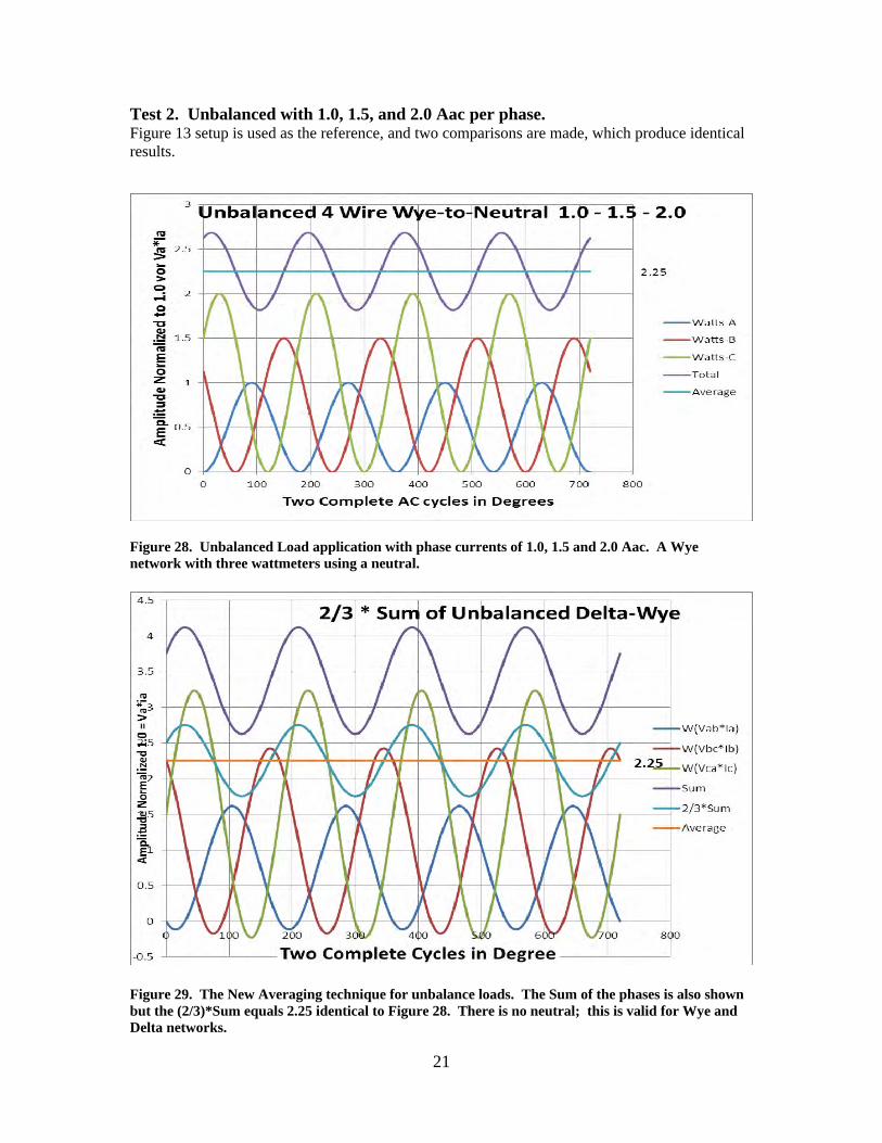
Test 2. Unbalanced with 1.0, 1.5, and 2.0 Aac per phase. Figure 13 setup is used as the reference, and two comparisons are made, which produce identical results.

Figure 28. Unbalanced Load application with phase currents of 1.0, 1.5 and 2.0 Aac. A Wye network with three wattmeters using a neutral.

Figure 29. The New Averaging technique for unbalance loads. The Sum of the phases is also shown but the (2/3)*Sum equals 2.25 identical to Figure 28. There is no neutral; this is valid for Wye and Delta networks.

22

Test 3, Unbalanced with extreme current for Phase C. The same test equipment setup but different phase currents. Note the effect is identical.

Figure 30. Unbalanced Reference using a 4-wire Wye with a neutral. Note the average is 6.0.

Figure 31. Unbalance Wye or Delta with Ia=1.0; Ib=1.0: and Ic =10.0. Note the average for 2 ac cycles is 6.0 which is identical to Figure 30.

23

Test 4, Ia=10.0, Ib=10.0, and Ic=1.0 Final test of unbalanced load conditions.

Figure 32. An Extreme Unbalance Condition

Figure 33. This three wattmeter approach is identical to Figure 32.

24

Conclusion of Test1, Test 2, Test 3, and Test 4 Four different scenarios were presented including balance and unbalance currents in a electrical distribution system. In all cases the use of a three wattmeter system produced the identical results as a four wire Wye with a neutral. This means that it does not matter if there is a Wye (Y) or Delta (Δ) three phase (3Φ) power balanced or unbalance true wattage is obtained with this method. This eliminates any confusion on the part of the designer as to what method is accurate. Equation 3 is shown again.

⎟⎠

⎞⎜⎝

⎛++= ∑

=

N

iiCiCiBiBiAiAN IVIVIVWatts

1

132 )*()*()*(( Equation 3

Where A, B, and C are the different Phases. These are line to line voltages, no neutral is needed. N is the number of samples for a complete cycle

Figure 34. Practical Example of the Three Wattmeter Approach. This is valid for Delta or Wye configurations. This example uses CT’s which could be replace with Shunt Resistors. Summary of Electrical Distributions Systems A summary of the various electrical distribution systems is given in Figure 35. This was taken from the “Handbook for Electricity Metering” (ISBN 0-931032-52-0). The common

25

names are given for each and the normal distribution voltages are also presented. One of the unique systems is the “Three-Phase Four-Wire Delta”, which will is sometimes referred to as a Three-Phase Center Tapped Delta. The National Electrical Code (NEC 2002) Handbook 2002 (ISBN 087765462-X) referees to these as “3-phase, 4wire Delta grounded system” and “3-phase grounded Delta system”. This configuration as shown in Figure 34 is one method that an unbalanced distribution system can exist. This Three-Phase Four-Wire Delta cannot be metered using the standard two-wattmeter approach presented in Figure 14 and Figure 15. The only way to obtain simple accurate metering is to use the approach shown in Figures 25 and 26. This approach does not need a ground or neutral connection. The meter needs to be connected between the service transformer and the service panel before the distribution of electricity to the facility. Additional figures and diagrams are being generated to show loading and wattage. A 240 Vac line-line voltage will be used as shown in Figure 34. Loads will be for 120 Vac single phase, 240 Vac three phase, and a 208 Vac single phase for fluorescent lighting. It will be shown that the same results will occur as that presented by Test 1, 2, 3 and 4.

26

Figure 35. Distribution configurations from the Electrical Handbook. This is Figure 4-31. Creating a Neutral Reference with a Delta Input A three wattmeter configuration that starts with a Delta (Δ) can be made using a Wye (Y) metering connection by creating a neutral. If the input utility power is from a Delta: Phase A, Phase B, and Phase C, an artificial type of neutral, NA, can be created. This new reference is to be used only for low current reference measurements. The new neutral, let us call it an artificial neutral and label it NA, can be created by taking resistors from each of the phases and joining them, this is shown in Figure 36. The creation of the artificial neutral eliminates the 2/3 factor in

27

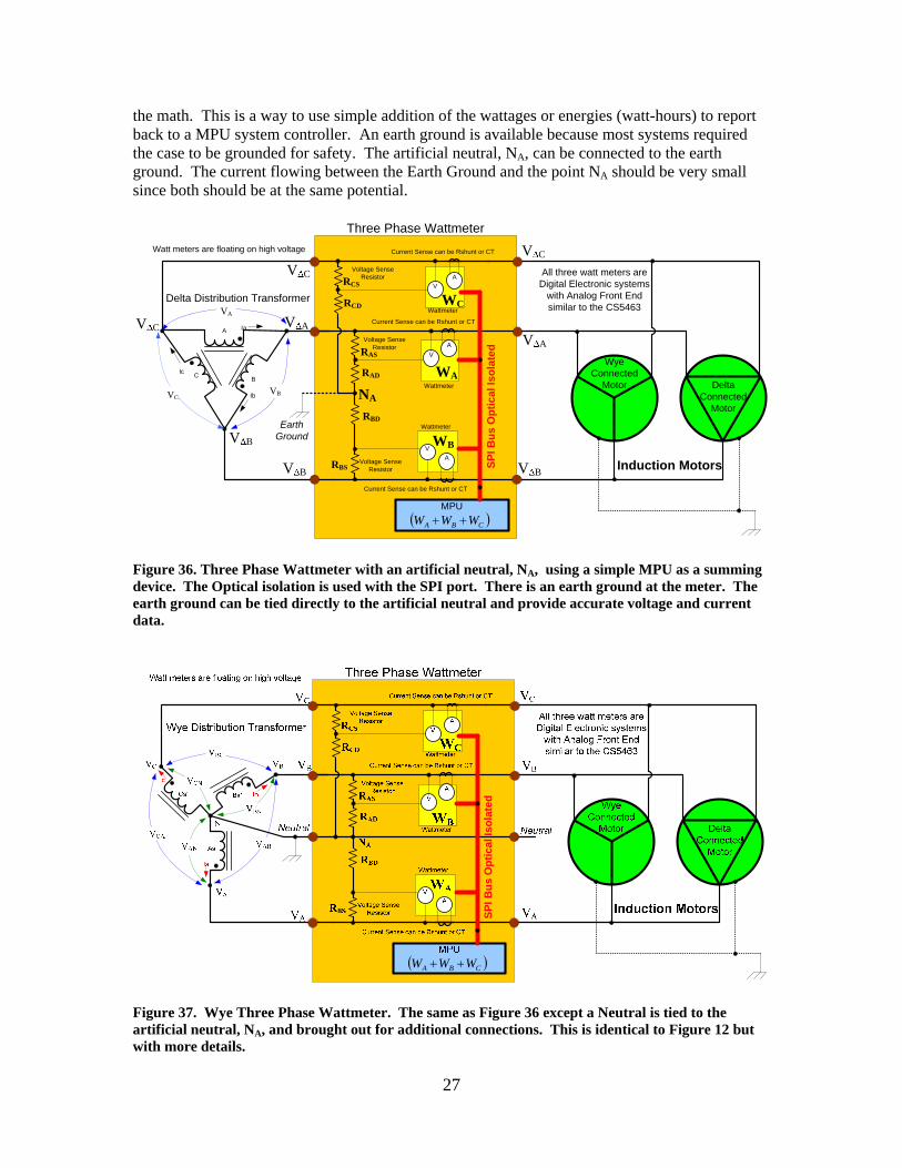
the math. This is a way to use simple addition of the wattages or energies (watt-hours) to report back to a MPU system controller. An earth ground is available because most systems required the case to be grounded for safety. The artificial neutral, NA, can be connected to the earth ground. The current flowing between the Earth Ground and the point NA should be very small since both should be at the same potential.

AV

Wattmeter

AV

Wattmeter

Wye Connected

Motor Delta Connected

Motor

Induction Motors

Watt meters are floating on high voltage

AV

Wattmeter

MPUSP

I Bus

Opt

ical

Isol

ated

All three watt meters are Digital Electronic systems

with Analog Front End similar to the CS5463

A

BC

Ia

Ib

Ic

VCVB

VA

Delta Distribution Transformer

V A

V B

V C

WA

WC

WB

NA

RCD

RCS

RAS

RAD

RBS

RBD

( )CBA WWW ++

Current Sense can be Rshunt or CT

Current Sense can be Rshunt or CT

Current Sense can be Rshunt or CT

Voltage Sense Resistor

Voltage Sense Resistor

Voltage Sense Resistor

Three Phase Wattmeter

V C

V C

V A

V B V B

Earth Ground

Figure 36. Three Phase Wattmeter with an artificial neutral, NA, using a simple MPU as a summing device. The Optical isolation is used with the SPI port. There is an earth ground at the meter. The earth ground can be tied directly to the artificial neutral and provide accurate voltage and current data.

SPI B

us O

ptic

al Is

olat

ed

( )CBA WWW ++

Figure 37. Wye Three Phase Wattmeter. The same as Figure 36 except a Neutral is tied to the artificial neutral, NA, and brought out for additional connections. This is identical to Figure 12 but with more details.

28

The design of the neutral point is very easy. There is a burden current created when this approach is used. The burden is the wattage of the resistors used to create this new reference point. There are two common Delta configurations used in North America: 240 Vac and 480 Vac. The 480 Vac has a 277 VacLN line to neutral voltage the same as a 480 Vac Wye (Y). The high line or worse case is 305 Vac. This means there is 305 Vac across each major set of resistors: RA series, RB series, and RC series. The resistors are made up of two resistors in series like RBS and RBD. The value of large value resistor is called the dropping resistor while the value of the small value resistor is called the sense resistor. The sense resistor is chosen so that its maximum voltage is 150 mVrms at the maximum value of line voltage. The maximum wattage is something arbitrary like 0.5 Watts per leg. So the total resistance of a leg is definesd below.

LEG

MAXlegperTotal Wattage

VoltageR2

=−− = Ω= 1860505.0

3052

The total burden for the wattmeter would be 3*0.5 Watt = 1.5 Watts. In order to have a good balance, the resistors chosen should be tight tolerance variety that

has a tolerance of 0.1%. The sense resistor would be on the order of a 100 ohm resistor with a tolerance of 0.1% or tighter. It would be recommended that the dropping resistor consist of four resistors in series so as to not exceed the voltage rating of the resistors and a transient voltage spike not jump across the resistor causing a carbon arc path. Third Order Harmonics Being Cancled. One of the unique benefits for using a three phase electrical power transmission system is the ability to have some of the harmonics cancel. This cancellation is for both voltage and current. This is the case for the odd triplets which include the third, ninth, fifteenth, etc. The cancellation occurs when a Wye to Delta transformer or Delta to Wye transformer is used to step up or step down the voltage. These types of harmonics are created when a bridge rectifier and large electrolytic capacitor are used to create a dc link. There are single phase bridge circuits and three phase bridge rectifier circuits; these are shown below in Figure 38. There are two other common rectifier circuits not shown: voltage-doubler and the half-wave rectifier circuit.

Figure 38. Common Rectifier Circuits Used Today

When the input current is measured using a low frequency spectrum analyzer an amplitude verses frequency plot is the result. The input current from a switching power supply for a desk top computer tower was measured. The result is shown in Figure 39. The power

29

supply was a non-power factor corrected type. The individual current harmonics are labeled. Please note the third and fifth order harmonics are nearly the same amplitude as the fundamental. The spectrum analyzer only presents the amplitude and not the phase relationship to fundamental. This is important because the phase is the other half of the data.

Figure 39. Frequency Spectrum of Current Harmonics. The current harmonics from the ac line using a non-power factor corrected computer power supply.

30

Figure 40. Three Phase System, Delta to Wye Transformer with Wattmeters, Service Panel and Loads. If there are three loads: Load A, Load B, and Load C. The loads have a single phase bridge rectifier circuit, see Figure 38, This creates current harmonics similar to that shown in Figure 39. The current is being supplied by a Wye (Y) distribution transformer; the distribution transformer has a neutral which can be seen and is labeled as a neutral in the Figure 40C. The actual core of this transformer appears as indicated below in the Figure 40A and 40B. Each of the phases has its own leg on the core, Figure 40A. There is a primary and a secondary winding for each of the phases. The primary and secondary windings are connected as shown in Figure 40C. The simple symbol for the Delta to Wye transformer is shown as Figure 40B. For this explanation the transformer winding ratio is 1:1. In practice the turns ration would be such to cause a 13.2 KVac (Primary-VLL) and a 120 Vac (Secondary- VLN), which is a 208 three phase (3Φ-VLL) line to line voltage. The label ‘Ia’ is current on the secondary reflecting to the ‘Ia’ current on the primary. If the load was a three phase bridge rectifier it would have the third order harmonic added to the fundamental. From the magnitude of the current shown in Figure 39, the amplitude of the fundamental current and the third order harmonic current have similar amplitudes. The third order harmonic current can be in phase or out of phase with the fundamental. The Spectrum Analyzer does not reveal any phase relationship. An excel spreadsheet was used to generate an in-phase plot of the fundamental and the third order harmonic current for the secondary current for Phase A, which is shown in Figure 41. A third order in-phase harmonic is generated using three phase bridge rectifier systems; this is often associated with variable speed motor drives. In this example the fundamental and the third order each have magnitude of 1.0 Aac rms. The effective rms current flowing in the secondary is

2 Aac.

31

....23

22

21

2 ++++= IIIII DCrms Equation 4 Where IDC = 0 Adc, I2 = 0 Aac I1 = 1.0 Aac I3 = 1.0 Aac

When the third order harmonic is out of phase with the fundamental the phase current is different. Most single phase rectifier circuits have a pulse of current at near the 90o point of the ac line voltage waveform. (See Figure 42 for actual phase current and neutral current.) If only the fundamental and third order out-of-phase current were present, and no other harmonics. The rms current would 2 Aac. A unique waveform results as shown as the red trace in Figure 43. If all three branch circuits: Phase A, Phase B, and Phase C, had the same load there would be a neutral current. The amplitude of the neutral current would be three times the magnitude of the fundamental current, green trace in Figure 43. Also note the third order harmonic is in phase with the neutral current. The neutral current has an amplitude of 3 Aac-peak. There is no fundamental current present in the neutral only third order harmonic current.

When these branch circuits: Phase A, Phase B, and Phase C, are connected to the distribution transformer the harmonics of the third, ninth, fifteenth, etc. cancel if their amplitudes for each harmonic are identical. This only can occur if the secondary is a Wye and the primary is a Delta. The same effect occurs for voltage harmonic generation at the power generation plant. There are harmonic voltages generated because the stator output has harmonics due to the construction of the stator and armature. The first stage after the generator is a Wye to Delta transformer, used to set-up the voltage and step-down the current in addition to eliminating the odd-triplet harmonic voltages. An attempt will be made to show the effect using an excel spreadsheet and graphs, and not the use of heavy math and trigonometric identities.

Figure 41. Phase A, Secondary Current, which is the fundamental plus the third order harmonic in phase with the fundamental of the same amplitude. This shows two humps in the current which is what is seen in three phase rectification occurs for variable speed motor drives.

32

Figure 42. Harmonic Distortion added to the neutral. Lower Trace is Phase A current while the upper trace is the neutral current. The third order harmonics add in the neutral.

Figure 43. Fundamental plus the third order harmonic of the same value as the fundamental but is 180 degrees our of phase with the fundamental. The neutrl current is now additive for all three phases and is large in amplitude than the fundamental current. The fundamental current in the neutral cancels so only the third order harmonic current is present. An attempt to show the harmonics do cancle will require the use of Figure 40. The turns ration of the transformer is 1:1 so whatever current flows in the secondary will flow also in the primary. The assumption is that all three brances: Phase A, Phase B, and Phase C have equal amplitudes of fundamental and third order out-of-phase harmonic current. The rms current for each phase is

2 Aac. On the primary side of the transformer there are two currents that will be used: Phase A and Phase C.

33

Math

On the primary side of the Delta transformer at the point, VΔC, there are three currents that combine to add to zero, Kirchhoff’s Current Law, please referee to Figure 40 for the point VΔC.

0=++ ΔCCa III Equation 5

where )3sin(sin tLtKIa ωω += , third order in-phase

)120(3sin()120sin( ooc tLtKI +++= ωω , third order in-phase

K and L are equal to 1 in this example but can be any value. In this example the current flowing into the dot is positive while the current flowing out

of the dot will be negative. After performing some simple algebra, the following equation results, see Equation 6 and Equation 7.

aCC III −=Δ Equation 6

)3sin(sin)120(3sin()120sin( tLtKtLtKI ooC ωωωω −−+++=Δ Equation 7

Using an excel spread sheet with amplitudes set to 1.0 the for Ia, and Ic can be created

with third order harmonics set to the same amplitude. In this example both Phase A and Phase C, are using a negative, out-of-phase, third order harmonic. The waveform for each phase is that shown in Figure 44. The Blue trace is Ia current in both the primary and secondary of the transformer, the red is the Ic current in both the primary and secondary of the transformer. The third order harmonics cancel and what results is a clean waveform, green, trace. Note the amplitude of the current flowing down the transmission line is 3 Apeak =1.73 Aac-peak. This is the same amplitude flowing down each of the other two lines. The third order harmonic currents cancel.

Transformer Heating

Harmonics generated by electronic load cause heating issues in the utility distribution transformers. Care must be taken to reduce harmonic current amplitude by various power factor correction techniques. The harmonic current flows in both the primary and secondary windings of the transformer. This harmonic current causes heating of the distribution transformers has created issues with the utility supply transformer blowing. This is the main reason for the Power Factor Correction specification for harmonic current limits.

34

Figure 44. Third Order Harmonic Currents Cancel. Only the fundamental current is transmitted on the primary side of the transformer. Measuring Harmonic Effects The harmonic currents produce harmonic powers. The Cirrus Logic CRD5463PM demo board has the ability to measure the effects of the various harmonics. When the CRD5463PM is measuring a load that has a single phase bridge rectifier harmonics are generated as shown in Figure 39. Some of the harmonic powers can be obtained, Figure 45 shows the screen shot of GUI interface for the CRD5463PM. The top block called TOTAL POWER shows the standard Vrms, Arms, Watt (Average Watts as defined by Equation 1), Var (Voltage Amps Reactive), VA (Apparent Power (S)), and PF (power factor).

The next lower box area, shows FUNDAMENTAL POWER. The watts defined really come from the Fourier Series that define watts by the following equation.

.....333222111 ++++= θθθ CosIVCosIVCosIVIVW DCDCatts Equation 8

Where Watt = 111 θCosIV Var = 111 θSinIV The frequency in Hertz is self-explanatory. The next block is the HARMONIC POWER. This is the sum of remaining harmonic powers. This is defined as the following equation. ...444333222111 +++=−= θθθθ CosIVCosIVCosIVCosIVWW attsharmonics Equation 9 Doing a little more algebra, the Total Harmonic Distortion (THD) for current can be calculated on a first order basis. The total first part is to assume there is very little harmonic power. In the above case the harmonic power of -0.373 is 1.584% which is small. Now using Equation 8 and assuming that this is only fundamental power.

35

Figure 45. GUI Interface for the CRD5463PM 111 θCosIVWatts = Equation 10 Where V1 = Vrms

lPowerFundamenta

VarCosIVSinIV 1

111

1111tan ==

θθθ Equation 11

1

11 tanarctan θθθ −== Equation 12

Power Factor = PFdisplacement* PFdistortion Equation 13 The PF displayed in Figure 44 is the combined effect of displacement power factor and distortion power factor. The displacement power factor is the effective angle between the fundamental current and fundamental voltage. PFDisplacement = 1θCos after 1θ is determined by Equations 11 and 12 ntdisplacemedistortionrmsrmsatts pfpfIVW **= Equation 14 PF = pfdistortion * pfdisplacement Equation 15

1

121 +

=THD

CosIVWatts rmsrms θ Equation 16

122

1 +=⎟⎟⎠

⎞⎜⎜⎝

⎛THD

WCosIV

atts

rmarms θ Equation 17

36

⎟⎟

⎠

⎞

⎜⎜

⎝

⎛−⎟⎟

⎠

⎞⎜⎜⎝

⎛= 1

2

1

atts

rmsrms

WCosIVTHD θ

Equation 18

The CS5463 is able to provide information to a MPU or a DSP to calculate the Total Harmonic Distortion.

In this example the displacement angle is -17.45o

⎟⎟⎟⎟⎟

⎠

⎞

⎜⎜⎜⎜⎜

⎝

⎛

−= −

919.23519.7tan 1

The THD = 7068.11547.23

519.17412.0517.118 2

=⎟⎟⎠

⎞⎜⎜⎝

⎛−⎟

⎠⎞

⎜⎝⎛ −∗∗ Cos

THD of 1.7068 = 170.68% The CRD5463PM can be used as a bench wattmeter allowing engineers to calculate THD without the use of an expensive electronic wattmeter.

37

Appendix A

12 Vac rms 2 Aac rms Instant Watts

Degrees Voltage Current Watts

0 0.0000 0.0000 0.0000 Voltage is I2*SQRT(2)*SIN(H5*PI()/180)

10 2.9469 0.4912 1.4474 Current is 2*SQRT(2)*SIN(A5*PI()/180)

20 5.8043 0.9674 5.6149 Watts is the product of Vac * Iac

30 8.4853 1.4142 12.0000 Average Watts is the sum of Watts/36

40 10.9085 1.8181 19.8324

50 13.0002 2.1667 28.1676

60 14.6969 2.4495 36.0000

70 15.9471 2.6579 42.3851

80 16.7127 2.7855 46.5526

90 16.9706 2.8284 48.0000

100 16.7127 2.7855 46.5526

110 15.9471 2.6579 42.3851

120 14.6969 2.4495 36.0000

130 13.0002 2.1667 28.1676

140 10.9085 1.8181 19.8324

150 8.4853 1.4142 12.0000

160 5.8043 0.9674 5.6149

170 2.9469 0.4912 1.4474

180 0.0000 0.0000 0.0000

190 -2.9469 -0.4912 1.4474

200 -5.8043 -0.9674 5.6149

210 -8.4853 -1.4142 12.0000

220 -10.9085 -1.8181 19.8324

230 -13.0002 -2.1667 28.1676

240 -14.6969 -2.4495 36.0000

250 -15.9471 -2.6579 42.3851

260 -16.7127 -2.7855 46.5526

270 -16.9706 -2.8284 48.0000

280 -16.7127 -2.7855 46.5526

290 -15.9471 -2.6579 42.3851

300 -14.6969 -2.4495 36.0000

310 -13.0002 -2.1667 28.1676

320 -10.9085 -1.8181 19.8324

330 -8.4853 -1.4142 12.0000

340 -5.8043 -0.9674 5.6149

350 -2.9469 -0.4912 1.4474

360 0.0000 0.0000 0.0000

24 Average Watts

38

   

Appendix B

Degrees Van Vbn Vcn Ia Ib Ic Total Watts Watts-A Watts-B Watts-C Total

0 0.000 0.866 -0.866 0.000 0.866 -0.866 1.5 0.000 0.750 0.750 1.5

15 0.259 0.707 -0.966 0.259 0.707 -0.966 1.5 0.067 0.500 0.933 1.5

30 0.500 0.500 -1.000 0.500 0.500 -1.000 1.5 0.250 0.250 1.000 1.5

45 0.707 0.259 -0.966 0.707 0.259 -0.966 1.5 0.500 0.067 0.933 1.5

60 0.866 0.000 -0.866 0.866 0.000 -0.866 1.5 0.750 0.000 0.750 1.5

75 0.966 -0.259 -0.707 0.966 -0.259 -0.707 1.5 0.933 0.067 0.500 1.5

90 1.000 -0.500 -0.500 1.000 -0.500 -0.500 1.5 1.000 0.250 0.250 1.5

105 0.966 -0.707 -0.259 0.966 -0.707 -0.259 1.5 0.933 0.500 0.067 1.5

120 0.866 -0.866 0.000 0.866 -0.866 0.000 1.5 0.750 0.750 0.000 1.5

135 0.707 -0.966 0.259 0.707 -0.966 0.259 1.5 0.500 0.933 0.067 1.5

150 0.500 -1.000 0.500 0.500 -1.000 0.500 1.5 0.250 1.000 0.250 1.5

165 0.259 -0.966 0.707 0.259 -0.966 0.707 1.5 0.067 0.933 0.500 1.5

180 0.000 -0.866 0.866 0.000 -0.866 0.866 1.5 0.000 0.750 0.750 1.5

195 -0.259 -0.707 0.966 -0.259 -0.707 0.966 1.5 0.067 0.500 0.933 1.5

210 -0.500 -0.500 1.000 -0.500 -0.500 1.000 1.5 0.250 0.250 1.000 1.5

225 -0.707 -0.259 0.966 -0.707 -0.259 0.966 1.5 0.500 0.067 0.933 1.5

240 -0.866 0.000 0.866 -0.866 0.000 0.866 1.5 0.750 0.000 0.750 1.5

255 -0.966 0.259 0.707 -0.966 0.259 0.707 1.5 0.933 0.067 0.500 1.5

270 -1.000 0.500 0.500 -1.000 0.500 0.500 1.5 1.000 0.250 0.250 1.5

285 -0.966 0.707 0.259 -0.966 0.707 0.259 1.5 0.933 0.500 0.067 1.5

300 -0.866 0.866 0.000 -0.866 0.866 0.000 1.5 0.750 0.750 0.000 1.5

315 -0.707 0.966 -0.259 -0.707 0.966 -0.259 1.5 0.500 0.933 0.067 1.5

330 -0.500 1.000 -0.500 -0.500 1.000 -0.500 1.5 0.250 1.000 0.250 1.5

345 -0.259 0.966 -0.707 -0.259 0.966 -0.707 1.5 0.067 0.933 0.500 1.5

360 0.000 0.866 -0.866 0.000 0.866 -0.866 1.5 0.000 0.750 0.750 1.5

This is Wye distribution system with the three voltages, currents, and wattages shown for a complete ac line cycle. This is a balanced system and is an equipment setup as shown in Figure 12 in the above text.

39

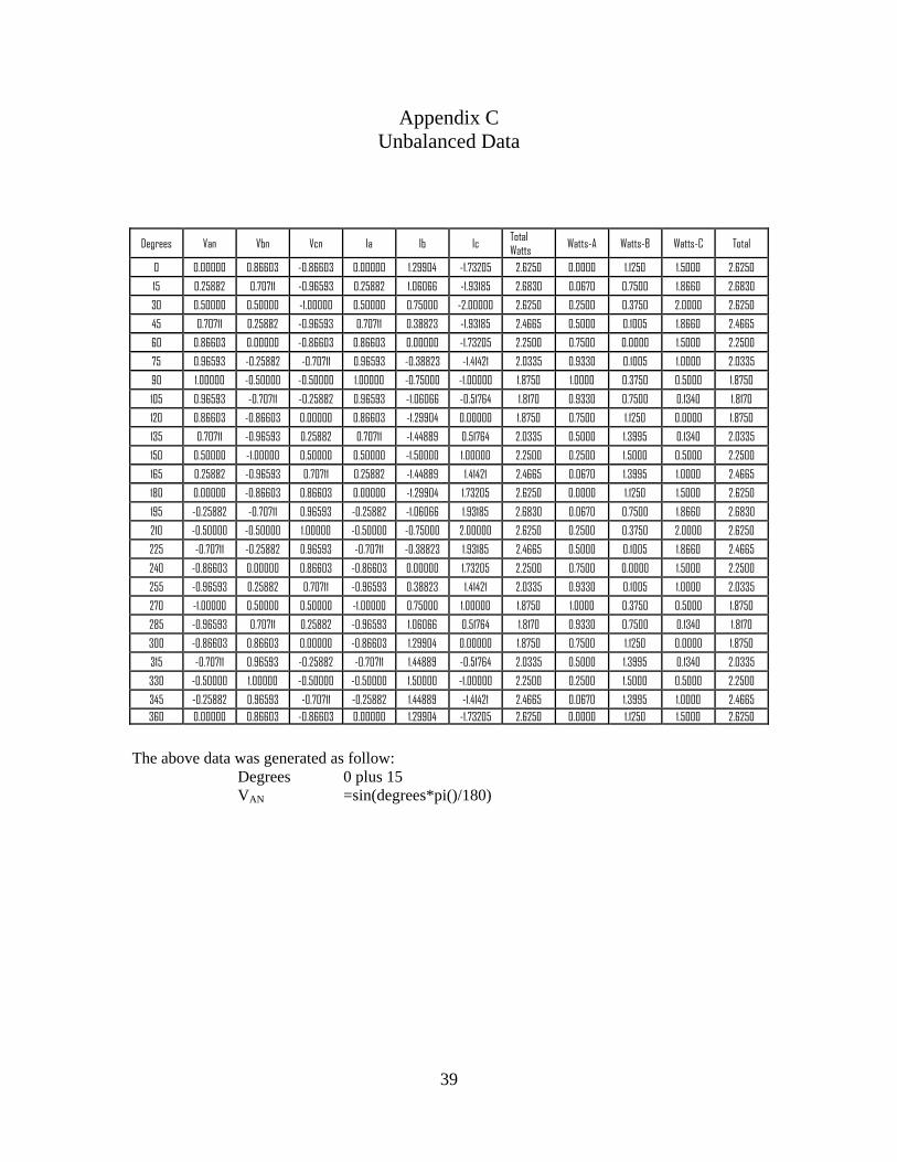
Appendix C Unbalanced Data

The above data was generated as follow:

Degrees 0 plus 15 VAN =sin(degrees*pi()/180)

Degrees Van Vbn Vcn Ia Ib Ic Total Watts

Watts-A Watts-B Watts-C Total

0 0.00000 0.86603 -0.86603 0.00000 1.29904 -1.73205 2.6250 0.0000 1.1250 1.5000 2.6250

15 0.25882 0.70711 -0.96593 0.25882 1.06066 -1.93185 2.6830 0.0670 0.7500 1.8660 2.6830

30 0.50000 0.50000 -1.00000 0.50000 0.75000 -2.00000 2.6250 0.2500 0.3750 2.0000 2.6250

45 0.70711 0.25882 -0.96593 0.70711 0.38823 -1.93185 2.4665 0.5000 0.1005 1.8660 2.4665

60 0.86603 0.00000 -0.86603 0.86603 0.00000 -1.73205 2.2500 0.7500 0.0000 1.5000 2.2500

75 0.96593 -0.25882 -0.70711 0.96593 -0.38823 -1.41421 2.0335 0.9330 0.1005 1.0000 2.0335

90 1.00000 -0.50000 -0.50000 1.00000 -0.75000 -1.00000 1.8750 1.0000 0.3750 0.5000 1.8750

105 0.96593 -0.70711 -0.25882 0.96593 -1.06066 -0.51764 1.8170 0.9330 0.7500 0.1340 1.8170

120 0.86603 -0.86603 0.00000 0.86603 -1.29904 0.00000 1.8750 0.7500 1.1250 0.0000 1.8750

135 0.70711 -0.96593 0.25882 0.70711 -1.44889 0.51764 2.0335 0.5000 1.3995 0.1340 2.0335

150 0.50000 -1.00000 0.50000 0.50000 -1.50000 1.00000 2.2500 0.2500 1.5000 0.5000 2.2500

165 0.25882 -0.96593 0.70711 0.25882 -1.44889 1.41421 2.4665 0.0670 1.3995 1.0000 2.4665

180 0.00000 -0.86603 0.86603 0.00000 -1.29904 1.73205 2.6250 0.0000 1.1250 1.5000 2.6250

195 -0.25882 -0.70711 0.96593 -0.25882 -1.06066 1.93185 2.6830 0.0670 0.7500 1.8660 2.6830

210 -0.50000 -0.50000 1.00000 -0.50000 -0.75000 2.00000 2.6250 0.2500 0.3750 2.0000 2.6250

225 -0.70711 -0.25882 0.96593 -0.70711 -0.38823 1.93185 2.4665 0.5000 0.1005 1.8660 2.4665

240 -0.86603 0.00000 0.86603 -0.86603 0.00000 1.73205 2.2500 0.7500 0.0000 1.5000 2.2500

255 -0.96593 0.25882 0.70711 -0.96593 0.38823 1.41421 2.0335 0.9330 0.1005 1.0000 2.0335

270 -1.00000 0.50000 0.50000 -1.00000 0.75000 1.00000 1.8750 1.0000 0.3750 0.5000 1.8750

285 -0.96593 0.70711 0.25882 -0.96593 1.06066 0.51764 1.8170 0.9330 0.7500 0.1340 1.8170

300 -0.86603 0.86603 0.00000 -0.86603 1.29904 0.00000 1.8750 0.7500 1.1250 0.0000 1.8750

315 -0.70711 0.96593 -0.25882 -0.70711 1.44889 -0.51764 2.0335 0.5000 1.3995 0.1340 2.0335

330 -0.50000 1.00000 -0.50000 -0.50000 1.50000 -1.00000 2.2500 0.2500 1.5000 0.5000 2.2500

345 -0.25882 0.96593 -0.70711 -0.25882 1.44889 -1.41421 2.4665 0.0670 1.3995 1.0000 2.4665 360 0.00000 0.86603 -0.86603 0.00000 1.29904 -1.73205 2.6250 0.0000 1.1250 1.5000 2.6250

40

References 1. CS5463, Cirrus Logic Data Sheet, www.cirrus.com

2. Handbook for Electricity Metering, 10th Ed. Copyright 2002, Edison Electric

Institute, ISBN 0-931032-52-0 3. Bergen, Arthur R,; Power Systems Analysis, Prentice-Hall, Copyright 1986; ISBN 0-

13-687864-4 4. Roadstrum and Wolaver, Electrical Engineering for all Engineers; Harper & Row,

Copyright 1986, chapter 4, ISBN 0-06-350611-4 5. Nasar, Electrical Machines and Electromechanics, 2nd Ed. Schaum’s Outline Series,

McGraw-Hill, ISBN 0-07-0459994-0 6. Cathey &Nasar, Basic Electrical Engineering, 2nd Ed. Chapter 3, Schaum’s Outline

Series, McGraw-Hill, ISBN 0-07-011355-6 7. Chapman, Electric machinery Fundamentals, 4th Ed. McGraw-Hill, Copyright 2005,

ISBN 0-07-246523-9