Abstract

interested several researchers and utilities during the last decade, trying to achieve higherbit-rates and more reliable communication over the power lines. The main advantagewith power-line communication is the use of an existing infrastructure. Wires exist toevery household connected to the power-line network.

This thesis starts with a general introduction to power-line communication. Then anexisting application, communicating on a low-voltage grid, is investigated in order toobtain some knowledge of how the power line acts as a communication channel. We alsoexpose this system with a load, consisting of a set of industrial machines, to study thechange in communication channel quality. After these large-scale measurements wemeasure some channel characteristics in the same grid. Measurements of the noise leveland the attenuation, up to 16 MHz, are reported.

The power-line communication channel can, in general, be modeled as having a time-varying frequency-dependent signal-to-noise ratio over the communication bandwidth.The effect of non-white Gaussian noise on different receiver structures is studied, oneideal and one sub-optimal, and the importance of diversity (in frequency) is illustratedwhen the set of transmitter waveforms is fixed. We investigate robust, low-complexity,modulation methods which are able to handle unknown phase and attenuation, whichsimplifies the implementation of the receiver.

Finally we describe a communication strategy that eventually could be used for informa-tion transfer over the power-line communication channel. In doing this we combine cod-ing, frequency diversity and the use of sub-channels (similar to Orthogonal FrequencyDivision Multiplex). This is a flexible structure which can be upgraded and adapted tofuture needs.

This thesis is about power-line communication over the low-voltage grid, which has

i

Preface v

CHAPTER 1 Introduction 11.1 Power-Line Communications

1.2 Digital Communications1.2.1 System Model1.2.2 Bandwidth1.2.3 Diversity

1.3 The Power-Line as a Communication Channel1.3.1 Bandwidth Limitations1.3.2 Radiation of the Transmitted Signal1.3.3 Impedance Mismatches1.3.4 Signal-to-Noise-Ratio1.3.5 The Time-variant Behavior of the Grid1.3.6 A Channel Model of the Power-Line Communication Channel1.3.7 Summary

1.4 Thesis Outline

CHAPTER 2 Communication Channel Properties of the Low-voltage Grid 15

2.1 Introduction

2.2 The PLC-P System2.2.1 The Implementation in Påtorp2.2.2 The Communication in PLC-P2.2.3 The Communication Technique

2.3 Estimated Overall Performance of the Communication Channels

2.3.1 The Average Performance of the Channels2.3.2 The Number of Households Experiencing at Least One Re-transmission2.3.3 The Overall Re-transmission Probabilit y

2.4 Channel Performance Associated with Specific Cable-Boxes in the Grid

2.5 Load Profile2.5.1 Load Profile and Communication Channel Impairments

2.6 Conclusions

ii

CHAPTER 3 On the Effect of Loads on Power-Line Communications 31

3.1 Introduction

3.2 The Influence of the Load on the Communication3.2.1 The Influence of the Load when Connected to the Sub Station3.2.2 The Influence of the Load when Connected to a Cable-Box

3.3 Measurements of the Harmonic Voltages and Currents Introduced by the Load

3.3.1 The Harmonic Disturbance Introduced in the Grid3.3.2 The Propagation of the Harmonic Disturbances

3.4 Conclusions

CHAPTER 4 Measurements of the Characteristics of the Low-voltage Grid 41

4.1 Measurement Setup4.1.1 Measurement Devices4.1.2 Coupling Circuits

4.2 Measurement Techniques4.2.1 Noise Measurements4.2.2 Attenuation Measurements4.2.3 Theory of Power Spectrum Estimation

4.3 Outdoor Measurements in the 1-16 MHz Frequency Band

4.3.1 The Noise Leve4.3.2 The Attenuation

4.4 Outdoor Measurements in the 20-450 kHz Frequency Band

4.4.1 The Noise Level4.4.2 The Attenuation

4.5 Conclusions

CHAPTER 5 Receiver Strategies for the Power-Line Communication Channel 59

5.1 Introduction

5.2 Assumptions and the Communication System Model

5.3 Two Receiver Structures5.3.1 The Ideal Receiver5.3.2 The Suboptimal Receiver5.3.3 Comparisons of the Receiver Structures

iii

5.4 Conclusions

CHAPTER 6 A Modulation Method for the Power-Line Communication Channel 71

6.1 The Modulation Method6.1.1 The Transmitter6.1.2 Communication Channel6.1.3 The Receiver6.1.4 The Maximum Likelihood Decision Rule

6.2 Computer Simulations

6.3 Union Bound

6.4 Communication Aspects of the Power-Line Communication Channel

6.5 Conclusions

CHAPTER 7 Conclusions 97

Bibliography 99

v

Preface

This is the result of my work as a graduate student at the Department of InformationTechnology at Lund University. Parts of this thesis have been presented at conferences:

- L. Selander, T. I. Mortensen, G. Lindell, "Load Profile and Communication ChannelCharacteristics of the Low Voltage Grid", Proc. DistribuTECH DA/DSM Europe 98,London, U.K., 1998.

- L. Selander, T. I. Mortensen, "Technical and Commercial Evaluation of the IDAM Sys-tem in Ronneby, Sweden", Proc. NORDAC-98, Bålsta, Sweden, 1998.

- G. Lindell, L. Selander, "On Coding-, Diversity- and Receiver Strategies for the Power-line Communication Channel", Proc. 3rd International Symposium on Power-line Com-munications and its Applications, Lancaster, UK, 1999.

These papers correspond to the work presented in Chapter 2, 3 and 5, and was mainlydone during my first year as a Ph.D. student. The results from the second year are notpresented at any conference, and are entirely written for this thesis. These are shown inChapter 4 and 6. The thesis starts with an introduction to power-line communication andends with conclusions.

Parts of this material have also been presented in the following seminar:

- Communication Systems for the Low-voltage Grid, Seminar on Power Line Communi-cations, NESA A/S, Copenhagen, Denmark, 1998.

Acknowledgments

There are many people who have supported and encouraged me during these years. Thishave meant a lot to me and I am very grateful to all of you. I would like to take this

vi

opportunity to especially acknowledge the following people for their various contribu-tions to this thesis.

First I would like to thank all of the students I have had during the years 94-99. Teachinghas been the best part of this work and a major reason to why I became a Ph.D. student. Iam very grateful to Mats Cedervall, who let me be a teaching assistant for him in DigitalDesign, which gave me a good start. I am also thankful to Mats Brorsson who let meteach a whole range of courses at the department of Computer Engineering.

Göran Lindell, my supervisor, has supported my work during my Ph.D. studies from thevery first beginning. His ability to see the practical use of theoretical results has helpedme on the way. He has also been proofreading this thesis, and his comments and sugges-tions, during these years, have been very educational and inspiring.

I am going to miss the Ph.D. students at the department, with who I have had much fun. Iwould especially like to thank Ola Wintzell, who have joined me in different sport activ-ities and with whom I have had daily non-research discussions.

Everyone at the technical staff at the department of Information Technology has been agreat help during these two years, something I thank them for. Especially Ilia Bol-anowski, who have contributed to this project in many ways: supplied me with compo-nents, technical support, discussions about research and life in general, and being a goodfriend. Lennart Magnusson has assisted me in many ways, servicing my, not alwaysfunctioning, equipment and contributing with his knowledge concerning technicalissues. I am certainly going to miss being a teaching assistant with you both.

I would also like to thank some of the people at the former department of ComputerEngineering: Jan Eric Larsson, Mats Brorsson, Fredrik Dahlstrand and Bengt Öhman,who I have had a lot in common with. Fredrik and Bengt have always been open for dis-cussions and fun. I would also like to take this opportunity to recommend Jan Eric'scourse in thesis reading. Without that course this thesis would have looked much differ-ent.

Laila Lembke has been doing a great job supporting the project. Kamil Sh. Zigangirovand the rest of the staff at the department of Information Technology also deserve mygratitude for their support.

Ronneby Energi AB has supported this project in many ways. Anders Andersson, Chris-ter Förberg and Rolf Håkansson have helped me with many practical details concerningthe experiments in Ronneby. Especially Rolf has, with patience, put up with strangerequirements and questions from a non-electrician. The people in the Påtorp area alsohave to be acknowledged. They have, without complaints, woken up to the sound of awelding unit, and have put up with wires routed on their paths.

During my first year I spent a lot of time working with Tony Mortensen at NESA A/Sin Denmark. He helped me with the experiments in the Påtorp area and many ideas fromthis research have been generated through our discussions. Steen Munk, NESA A/S, alsoparticipated in these experiments.

vii

Richard Krejstrup, Mats Bäckström and Marko Krejic were of great help during my mea-surements in Påtorp, they helped me with my experiments and have contributed withmany ideas to this thesis.

I have had the opportunity of having regularly meetings with my sponsors. These meet-ings have put the research in a new perspective and have generated many ideas. Withoutthese meetings this project would have been very different. This work has been sup-ported by the Swedish National Energy Administration (Energimyndigheten) and byElforsk (supported by Sveriges Elleverantörer, Stiftelsen Ronneby Soft Center, TeliaResearch, EnerSearch AB, NESA A/S, Fortum Power and Heat). I would also like toacknowledge Hans Ottosson, head of EnerSearch AB, who initiated this project and hasbeen supporting this work at all times.

I would like to thank everyone at Hardi Electronics AB, who, after my decision to quitmy work at the department, offered me the best job anybody could get.

I would like to give a special thanks to some of my friends: Ola Sundberg and Tim Nel-son, for all get-togethers, playing the guitar, and all of the friends who have joined me inwinter bathing, especially, Mattias Hansson and Gunnar Dahlgren. I also thank theremainder of my friends for distracting me from this work.

My parents have supported me from pre-school to graduate studies and have in manyways inspired me in my work and guided me through life to the individual I am. Thesame goes for my brother.

Finally, I am very grateful to my wife Viveca, who in many ways have contributed to thiswork: proofreading, assisting me during the measurements in Påtorp, discussingresearch, and taking care of me when I have not had the time myself. I love you.

1

CHAPTER 1 Introduction

The communication flow of today is very high. Many applications are operating at highspeed and a fixed connection is often preferred. If the power utilities could supply com-munication over the power-line to the costumers it could make a tremendous break-through in communications. Every household would be connected at any time and ser-vices being provided at real-time. Using the power-line as a communication mediumcould also be a cost-effective way compared to other systems because it uses an existinginfrastructure, wires exists to every household connected to the power-line network.

The deregulated market has forced the power utilities to explore new markets to find newbusiness opportunities, which have increased the research in power-line communicationsthe last decade. The research has initially been focused on providing services related topower distribution such as load control, meter reading, tariff control, remote control andsmart homes. These value-added services would open up new markets for the power util-ities and hence increase the profit. The moderate demands of these applications make iteasier to obtain reliable communication. Firstly, the information bit rate is low, secondly,they do not require real-time performance.

During the last years the use of Internet has increased. If it would be possible to supplythis kind of network communication over the power-line, the utilities could also becomecommunication providers, a rapidly growing market. On the contrary to power relatedapplications, network communications require very high bit rates and in some cases real-time responses are needed (such as video and TV). This complicates the design of a com-munication system but has been the focus of many researchers during the last years. Sys-tems under trial exist today that claim a bit rate of 1 Mb/s, but most commerciallyavailable systems use low bit rates, about 10-100 kb/s, and provides low-demanding ser-vices such as meter reading.

The power-line was initially designed to distribute power in an efficient way, hence it isnot adapted for communication and advanced communication methods are needed.

2

Today’s research is mainly focused on increasing the bit rate to support high-speed net-work applications.

This thesis is about communication on the power-line (on the low-voltage grid). Section1.1 gives a general description of power-line communications. Section 1.2 explains somepreliminaries needed in digital communications and Section 1.3 describes the power-linechannel, its characteristics, problems and limitations, and also serves as a survey of cur-rent research. Finally Section 1.4 gives an outline of the rest of this thesis. Other intro-ductory descriptions on power-line communications are given in [14], [20], and [36].Reference [36] also studies new business opportunities for the power utilities and reportsresearch on coming technology.

1.1 Power-Line Communications

The power-line network is a large infrastructure covering most parts of the inhabitedareas. In Sweden the power is typically generated by, e.g., a power plant and then trans-ported on high-voltage (e.g., 400kV) cables to a medium-voltage sub station, whichtransforms the voltage into, e.g., 10kV and distributes the power to a large number oflow-voltage grids.

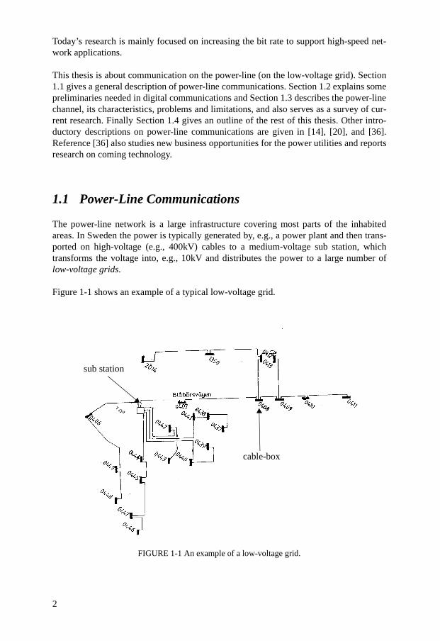
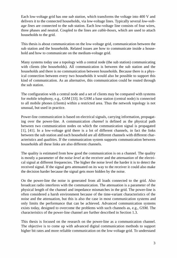
Figure 1-1 shows an example of a typical low-voltage grid.

FIGURE 1-1 An example of a low-voltage grid.

cable-box

sub station

3

Each low-voltage grid has one sub station, which transforms the voltage into 400 V anddelivers it to the connected households, via low-voltage lines. Typically several low-volt-age lines are connected to the sub station. Each low-voltage line consists of four wires,three phases and neutral. Coupled to the lines are cable-boxes, which are used to attachhouseholds to the grid.

This thesis is about communication on the low-voltage grid, communication between thesub station and the households. Related issues are how to communicate inside a house-hold and how to communicate on the medium-voltage grid.

Many systems today use a topology with a central node (the sub station) communicatingwith clients (the households). All communication is between the sub station and thehouseholds and there is no communication between households. Because there is a phys-ical connection between every two households it would also be possible to support thiskind of communication. As an alternative, this communication could be routed throughthe sub station.

The configuration with a central node and a set of clients may be compared with systemsfor mobile telephony, e.g., GSM [33]. In GSM a base station (central node) is connectedto all mobile phones (clients) within a restricted area. Thus the network topology is notunusual, but used in practice.

Power-line communication is based on electrical signals, carrying information, propagat-ing over the power-line. A communication channel is defined as the physical pathbetween two communication nodes on which the communication signal is propagated[1], [41]. In a low-voltage grid there is a lot of different channels, in fact the linksbetween the sub station and each household are all different channels with different char-acteristics and qualities. If the communication system supports communication betweenhouseholds all these links are also different channels.

The quality is estimated from how good the communication is on a channel. The qualityis mostly a parameter of the noise level at the receiver and the attenuation of the electri-cal signal at different frequencies. The higher the noise level the harder it is to detect thereceived signal. If the signal gets attenuated on its way to the receiver it could also makethe decision harder because the signal gets more hidden by the noise.

On the power-line the noise is generated from all loads connected to the grid. Alsobroadcast radio interferes with the communication. The attenuation is a parameter of thephysical length of the channel and impedance mismatches in the grid. The power-line isoften considered a harsh environment because of the time-variant characteristics of thenoise and the attenuation, but this is also the case in most communication systems andonly limits the performance that can be achieved. Advanced communication systemsexists today, designed to overcome the problems with such channels as, e.g., GSM. Thecharacteristics of the power-line channel are further described in Section 1.3.

This thesis is focused on the research on the power-line as a communication channel.The objective is to come up with advanced digital communication methods to supporthigher bit rates and more reliable communication on the low-voltage grid. To understand

4

the problem field some preliminaries are needed from digital communications. This isthe subject of the next section.

1.2 Digital Communications

In this section we study some preliminaries from digital communications. A model of adigital communication system is given in the next section and the last two sections give ashort introduction to bandwidth and diversity.

1.2.1 System Model

Figure 1-2 shows a simplified model of a digital communication system. Recommendedtextbooks on this subject are [1], [41] and [54]. The objective of the communication sys-tem is to communicate digital information (a sequence of binary information digits) overa noisy channel at as high bit rates as possible. The data to be transmitted could originfrom any source of information. In case the information is an analog signal, such asspeech, then an A/D converter must precede the transmitter.

FIGURE 1-2 A model of a digital communication system.

The source encoder outputs data that are to be transmitted over the channel at a certaininformation bit rate, Rb. As a measure of performance we define the bit error probability,Pb, as the probability that a bit is incorrectly received at the destination. As we will see

later, the channel may interfere with the communication, thus increasing the bit errorprobability.

Source Coding

Most data contains redundancy, which makes it possible to compress the data. This isdone by the source encoder and minimizes the amount of bits transmitted over the chan-nel. At the receiver the source decoder unpacks the data to either an exact replica of thesource (lossless data compression) or a distorted version (lossy data compression). If thereceived sequence does not have to be an exact copy of the transmitted stream then thedegree of compression can be increased.

Source

Destination

Channelencoder

Channeldecoder

Sourceencoder

Sourcedecoder

Modulator

Demodulator

Channel

5

Channel Coding

In order to reduce the bit error probability the channel encoder adds redundancy (extracontrol bits) to the bit sequence in a controlled way. When an error appears in the bitstream the extra information may be used by the channel decoder, to detect, and possiblycorrect, the error. The redundancy added is depending on the amount of correctionneeded but is also tuned to the characteristics of the channel.

Two coding techniques often used are block codes [41] and convolutional codes [27],[41].

Modulator

The modulator produces an information-carrying signal, propagating over the channel.At this stage the data is converted from a stream of bits into an analog signal that thechannel can handle. The modulator has a set of analog waveforms at its disposal andmaps a certain waveform to a binary digit or a sequence of digits. At the receiver, thedemodulator tries to detect which waveform was transmitted, and convert the analoginformation back to a sequence of bits.

Several modulation techniques exists, e.g., spread-spectrum [41], OFDM (OrthogonalFrequency Division Multiplex) [18], GMSK (Gaussian Minimum Shift Keying) [33],FSK (Frequency Shift Keying) [41], PSK (Phase Shift Keying) [41] and QAM (Quadra-ture Amplitude Modulation) [41].

Channel

The channel might be any physical medium, such as coaxial cable, air, water or tele-phone wires. It is important to know the characteristics of the channel, such as the atten-uation and the noise level, because these parameters directly affect the performance ofthe communication system.

1.2.2 Bandwidth

The frequency content of the information-carrying signal is of great importance. The fre-quency interval used by the communication system is called bandwidth, W [41]. For aspecific communication method, the bandwidth needed is proportional to the bit rate.Thus a higher bit rate needs a larger bandwidth for a fixed method. If the bandwidth isdoubled then the bit rate is also doubled.

In today’s environment bandwidth is a limited and precious resource and the bandwidthis often constrained to a certain small interval. This puts a restriction on the communica-tion system to communicate within the assigned bandwidth.

To compare different communication systems the bandwidth efficiency, ρ, is defined as

6

(1-1)

and is a measure of how good the communication system is [41]. Today, an advancedtelephone modem can achieve a bit rate of 56.6 kb/s using a bandwidth of 4 kHz and thebandwidth efficiency is 14.15 b/s/Hz. A meter reading system for the power-line channelthat has a bit rate of 10 kb/s and communicates within the CENELEC A band has a band-width efficiency of 0.11 b/s/Hz, thus the performance of the telephone modem is muchhigher.

1.2.3 Diversity

To reduce the error probability of harsh channels, diversity techniques [41] may be used.Examples are time diversity and frequency diversity.

In time diversity the same information is transmitted more than once at several differenttime instants. If the channel is bad at some time instant the information might passthrough at some other time when the channel is good (or better). This is especially usefulon time-varying channels.

Frequency diversity transmits the same information at different locations in the fre-quency domain. It can be compared to having two antennas transmitting at different fre-quencies, if one of them fail the other might work.

1.3 The Power-Line as a Communication Channel

In this section we study the power-line as a communication channel and discuss the cur-rent research. In Section 1.1 we defined a channel as a physical path between a transmit-ter and a receiver. Note that a low-voltage grid consists of many channels each with itsown characteristics and quality.

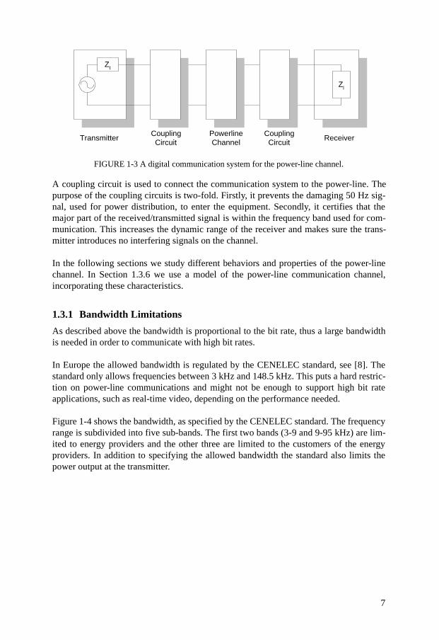
Figure 1-3 below shows a digital communication system using the power-line as a com-munication channel. The transmitter is shown to the left and the receiver to the right.Important parameters of the communication system are the output impedance, Zt, of thetransmitter and the input impedance, Zl, of the receiver.

ρRb

W------=

7

FIGURE 1-3 A digital communication system for the power-line channel.

A coupling circuit is used to connect the communication system to the power-line. Thepurpose of the coupling circuits is two-fold. Firstly, it prevents the damaging 50 Hz sig-nal, used for power distribution, to enter the equipment. Secondly, it certifies that themajor part of the received/transmitted signal is within the frequency band used for com-munication. This increases the dynamic range of the receiver and makes sure the trans-mitter introduces no interfering signals on the channel.

In the following sections we study different behaviors and properties of the power-linechannel. In Section 1.3.6 we use a model of the power-line communication channel,incorporating these characteristics.

1.3.1 Bandwidth Limitations

As described above the bandwidth is proportional to the bit rate, thus a large bandwidthis needed in order to communicate with high bit rates.

In Europe the allowed bandwidth is regulated by the CENELEC standard, see [8]. Thestandard only allows frequencies between 3 kHz and 148.5 kHz. This puts a hard restric-tion on power-line communications and might not be enough to support high bit rateapplications, such as real-time video, depending on the performance needed.

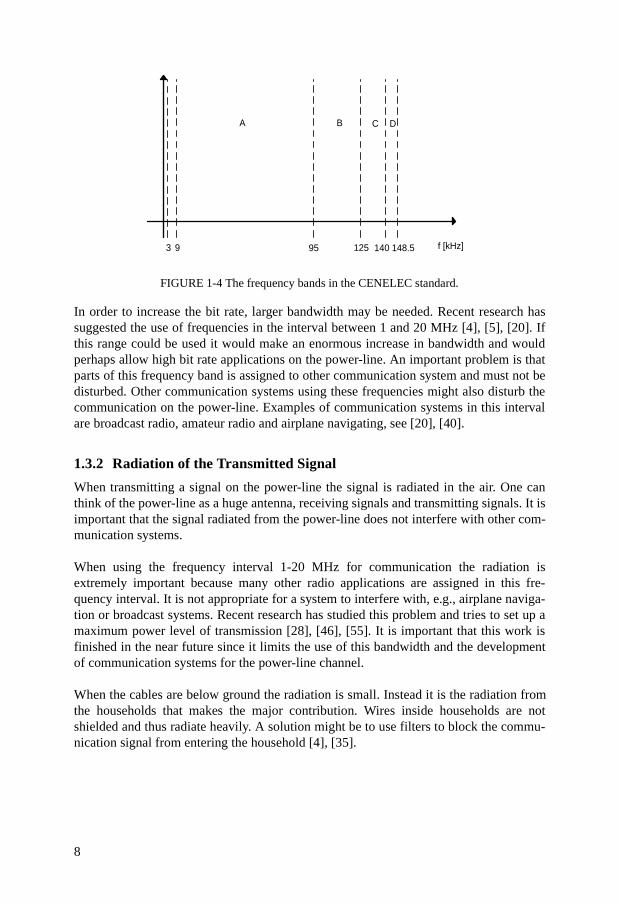
Figure 1-4 shows the bandwidth, as specified by the CENELEC standard. The frequencyrange is subdivided into five sub-bands. The first two bands (3-9 and 9-95 kHz) are lim-ited to energy providers and the other three are limited to the customers of the energyproviders. In addition to specifying the allowed bandwidth the standard also limits thepower output at the transmitter.

TransmitterCouplingCircuit

CouplingCircuit

PowerlineChannel

Receiver

Zt

Zl

8

FIGURE 1-4 The frequency bands in the CENELEC standard.

In order to increase the bit rate, larger bandwidth may be needed. Recent research hassuggested the use of frequencies in the interval between 1 and 20 MHz [4], [5], [20]. Ifthis range could be used it would make an enormous increase in bandwidth and wouldperhaps allow high bit rate applications on the power-line. An important problem is thatparts of this frequency band is assigned to other communication system and must not bedisturbed. Other communication systems using these frequencies might also disturb thecommunication on the power-line. Examples of communication systems in this intervalare broadcast radio, amateur radio and airplane navigating, see [20], [40].

1.3.2 Radiation of the Transmitted Signal

When transmitting a signal on the power-line the signal is radiated in the air. One canthink of the power-line as a huge antenna, receiving signals and transmitting signals. It isimportant that the signal radiated from the power-line does not interfere with other com-munication systems.

When using the frequency interval 1-20 MHz for communication the radiation isextremely important because many other radio applications are assigned in this fre-quency interval. It is not appropriate for a system to interfere with, e.g., airplane naviga-tion or broadcast systems. Recent research has studied this problem and tries to set up amaximum power level of transmission [28], [46], [55]. It is important that this work isfinished in the near future since it limits the use of this bandwidth and the developmentof communication systems for the power-line channel.

When the cables are below ground the radiation is small. Instead it is the radiation fromthe households that makes the major contribution. Wires inside households are notshielded and thus radiate heavily. A solution might be to use filters to block the commu-nication signal from entering the household [4], [35].

3 9 95 125 140 148.5 f [kHz]

A B C D

9

1.3.3 Impedance Mismatches

Normally, at conventional communication, impedance matching is attempted, such as theuse of 50 ohm cables and 50 ohm transceivers. The power-line network is not matched.The input (and output) impedance varies in time, with different loads and location. It canbe as low as milli Ohms and as high as several thousands of Ohms and is especially lowat the sub station [2], [24], [31], [34], [38], [53].

Except the access impedance several other impedance mismatches might occur in thepower-line channel. E.g., cable-boxes do not match the cables and hence the signal getsattenuated.

Recent research has suggested the use of filters stabilizing the network [35]. The cost ofthese filters might be high and they must be installed in every household and perhapsalso in every cable-box.

1.3.4 Signal-to-Noise-Ratio

A key parameter when estimating the performance of a communication system, is thesignal-to-noise power ratio, SNR [41]:

(1-2)

This parameter is related to the performance of a communication system. The higherSNR the better communication.

The noise power on the power-line is a sum of many different disturbances. Loads con-nected to the grid, such as TV, computers and vacuum cleaners generate noise propagat-ing over the power-line. Other communication systems might also disturb thecommunication, thus introducing noise at the receiver. Noise measurements are found in[2], [6], [15], [20], [24], [32], [38].

When the signal is propagating from the transmitter to the receiver the signal gets attenu-ated. If the attenuation is very high the received power gets very low and might not bedetected. The attenuation on the power-line has shown to be very high (up to 100 dB)and puts a restriction on the distance from the transmitter to the receiver [2], [15], [20],[24]. An option might be to use repeaters in the cable-boxes, thus increasing the commu-nication length.

The use of filters could improve the signal-to-noise ratio [35]. If a filter is placed at eachhousehold blocking the noise generated indoors from entering the grid, the noise level inthe grid will decrease, but the cost is a higher complexity.

It is important to point out that although the power-line is considered a harsh environ-ment when it comes to attenuation and disturbances, these parameters exists in any com-munication system used today.

SNRReceived power

Noise power--------------------------------------=

10

1.3.5 The Time-variant Behavior of the Grid

A problem with the power-line channel is the time-variance of the impairments, see e.g.,[2]. The noise level and the attenuation depend partly on the set of connected loads,which varies in time. A channel which is time-variant, complicates the design of a com-munication system. At some time instants the communication might work well but atother times a strong noise source could be inherent on the channel, thus blocking thecommunication.

To solve this a possible solution is to let the communication system adapt to the channel[41]. At any time the characteristics of the channel are estimated, e.g., through measure-ments, and the effect is evaluated to make a better decision. The cost of this is highercomplexity.

1.3.6 A Channel Model of the Power-Line Communication Channel

In the previous section we have seen some impairments that reduce the performance of apower-line communication system:

• Impedance mismatches at the transmitter

• Channel attenuation

• Disturbances (noise)

• Impedance mismatches at the receiver

• Time-variations of the impairments

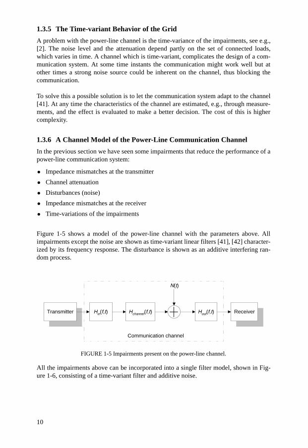
Figure 1-5 shows a model of the power-line channel with the parameters above. Allimpairments except the noise are shown as time-variant linear filters [41], [42] character-ized by its frequency response. The disturbance is shown as an additive interfering ran-dom process.

FIGURE 1-5 Impairments present on the power-line channel.

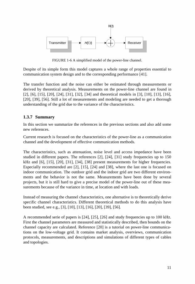
All the impairments above can be incorporated into a single filter model, shown in Fig-ure 1-6, consisting of a time-variant filter and additive noise.

Transmitter ReceiverHin(f,t) Hchannel(f,t) Hout(f,t)

N(t)

Communication channel

11

FIGURE 1-6 A simplified model of the power-line channel.

Despite of its simple form this model captures a whole range of properties essential tocommunication system design and to the corresponding performance [41].

The transfer function and the noise can either be estimated through measurements orderived by theoretical analysis. Measurements on the power-line channel are found in[2], [6], [15], [20], [24], [31], [32], [34] and theoretical models in [3], [10], [13], [16],[20], [39], [56]. Still a lot of measurements and modeling are needed to get a thoroughunderstanding of the grid due to the variance of the characteristics.

1.3.7 Summary

In this section we summarize the references in the previous sections and also add somenew references.

Current research is focused on the characteristics of the power-line as a communicationchannel and the development of effective communication methods.

The characteristics, such as attenuation, noise level and access impedance have beenstudied in different papers. The references [2], [24], [31] study frequencies up to 150kHz and [6], [15], [20], [31], [34], [38] present measurements for higher frequencies.Especially recommended are [2], [15], [24] and [38], where the last one is focused onindoor communication. The outdoor grid and the indoor grid are two different environ-ments and the behavior is not the same. Measurements have been done by severalprojects, but it is still hard to give a precise model of the power-line out of these mea-surements because of the variance in time, at location and with loads.

Instead of measuring the channel characteristics, one alternative is to theoretically derivespecific channel characteristics. Different theoretical methods to do this analysis havebeen studied, see e.g., [3], [10], [13], [16], [20], [39], [56].

A recommended serie of papers is [24], [25], [26] and study frequencies up to 100 kHz.First the channel parameters are measured and statistically described, then bounds on thechannel capacity are calculated. Reference [20] is a tutorial on power-line communica-tions on the low-voltage grid. It contains market analysis, overviews, communicationprotocols, measurements, and descriptions and simulations of different types of cablesand topologies.

Transmitter ReceiverH(f,t)

N(t)

12

The radiation problem is described in [28], [46], [55], which report measurements of theradiation and also try to set up a limit of the transmitter power.

Standardization of power-line communication in a regulatory perspective is found in [22]and a general discussion of different standards for power-line communication is given in[35].

Other papers dealing with most aspects of power-line communication can be found inProceedings from the International Symposium on Power-line Communications confer-ences, see [43], [44] and [45].

Different modulation methods have been proposed to be used on the low-voltage grid.Methods often considered as candidates are OFDM (Orthogonal Frequency DivisionMultiplex), spread-spectrum and GMSK (Gaussian Minimum Shift Keying). Thesemethods are described in [18], [41] and [33].

1.4 Thesis Outline

The remaining six chapters are concerned with different aspects of power-line communi-cations.

Chapter 2 Communication Channel Properties of the Low-voltage Grid

In this chapter we study some basic properties of the power-line channel. By observingan existing system using the low-voltage grid as a communication medium it is possibleto draw conclusions of how large-scale variations affect the communication, such as thevariation in time and energy usage in the grid. Also the performance of individual chan-nels are measured and related to the distance between the transmitter and the receiverand the location in the grid.

Chapter 3 On the Effect of Loads on Power-Line Communications

Loads change the condition of a grid. It is therefore interesting to study how this changeof state affects the communication. By using a moveable load source consisting of a setof industrial machines we have been able to relate the effect of this load to the degrada-tion of performance of a running communication system. It is also studied how the dis-tance to the load is related to quality of the channels.

Chapter 4 Measurements of the Characteristics of the Low-voltage Grid

To further explore the characteristics of the power-line, measurements have been done ina specific low-voltage grid. We show measurements of the noise level and the attenua-tion of the power-line channel. Frequencies in the bandwidth regulated by the CEN-ELEC standard [8] is studied, but also frequencies up to 16 MHz. The results are alsorelated to the performance analysis in Chapter 2.

13

Chapter 5 Receiver Strategies for the Power-Line Communication Channel

From the measurements in Chapter 4 it is clear that the noise level can not be modeled asan additive white gaussian noise process (AWGN) [41], thus it is non-white. (An AWGNprocess is characterized by the power being evenly distributed over the whole frequencyband). In this chapter we study the effect of this non-white noise on specific receiverstructures. Two receiver structures are compared with respect to robustness and narrow-band disturbances.

Chapter 6 A Modulation Method for the Power-Line Communication Channel

The experiments in Chapter 2 and 3 and the measurements in Chapter 4 imply that arobust modulation method might be used, robust against phase changes and attenuation.In this chapter we introduce a modulation method designed to support robustness. Themethod is a combination of FSK and PSK [41]. The error probability and the bandwidthefficiency of the method are calculated and compared to other robust methods.

In this chapter we also summarize the key result from previous chapters and try to usethis to design a communication system for the power-line. The outcome is a communica-tion strategy designed to support robustness and ease of implementation. Modulationmethods, coding and diversity are used.

Chapter 7 Conclusions

Here we conclude the thesis and report the key results.

15

CHAPTER 2 Communication Channel Properties of the Low-voltage Grid

2.1 Introduction

In order to design a communication system for a specific channel it is preferable to havesome basic knowledge of the characteristics of the channel. If a communication systemcan be matched to a channel, it increases the performance [41].

The intention with the project described in this chapter is to study the properties/behaviorof the communication channel by observing an existing system used on the low-voltagegrid in a typical application. Here we focus on large-scale variations of the communica-tion channel, e.g., how its quality depends on different time-windows, distances andloads.

It is well-known from communication theory that any practical communication systemwill have communication problems if the signal-to-noise ratio at the receiver dropsbelow a certain level [41]. This can of course happen also in the power-line communica-tion channel as a result of channel impairments, e.g., signal attenuation, signal degrada-tion and noise sources along the signal path. In the following the quality of a channel is ameasure of how good the communication system work.

In order to obtain quantitative results, parameters related to the quality of the communi-cation channel are estimated. The most frequently used parameter, in this chapter, is anestimate of the probability that re-transmissions of so-called transactions are made. Thisparameter is used as an indicator of the quality of the communication channel, since a re-transmission is made when the receiver is unable to make a reliable decision, which inturn normally is due to channel impairments. Hence, a low value on the probability of re-transmissions indicates a "good" communication channel.

It should be observed that the estimated probability above does not measure the reliabil-ity in the final decisions produced by the communication system. In general, a high reli-

16

ability in the final decisions can be obtained with communication systems using re-transmissions. However, the focus of this work is on the quality of the communicationchannel, and that is the reason why we estimate parameters that reflect how often chan-nel impairments result in re-transmissions.

The communication system we have used is located in Ronneby, Sweden, in an areacalled Påtorp. The system was chosen because it is in use within the project and it hasbeen tested on several locations in different environments. Furthermore it is fully imple-mented and commercially available. In the rest of this thesis we denote this system PLC-P (a Power-line Communication System in Påtorp).

The purpose has not been to evaluate the PLC-P system, but rather to extract informationfrom PLC-P that can be used to estimate the quality of the power-line as a communica-tion channel.

The disposition of this chapter is as follows:

• A description of the PLC-P system, Section 2.2.

• The overall performance of the communication channels in the low-voltage grid, Sec-tion 2.3.

• The performance of the communication channels at various locations in the low-volt-age grid, Section 2.4.

• The relation between the load profile and the quality of the communication channels,Section 2.5.

• Discussion and conclusions, Section 2.6.

Chapter 3 is related to the work in this chapter and studies the effect of loads on the com-munication, also using the PLC-P system as a reference.

2.2 The PLC-P System

The backbone of PLC-P is its possibility to support meter reading but it is also designedto support other services such as alarm systems. The structure of PLC-P is designed to bean open-system architecture and easily extendable to both producer and consumer spe-cific applications. PLC-P is also described in [49].

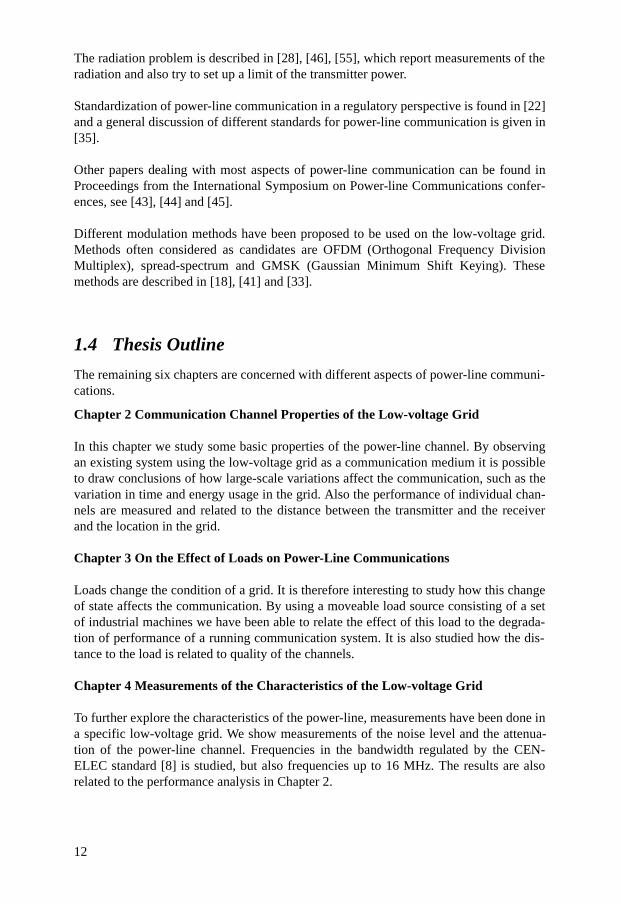
PLC-P consists of three major parts. The Multi Function Node (MFN), the Concentrator& Communication Node (CCN) and the Operation and Management System (OMS).Figure 2-1 shows how the parts are connected in a typical system.

17

FIGURE 2-1 The different parts of the PLC-P system and how they are connected.

The MFN is a unit that is installed in each household either as an integrated or separatepart of the meter. It reads the meter value each hour and stores it in a memory. The mem-ory can store up to 40 days of meter values.

The CCN manages all MFNs in an area, e.g., a low-voltage grid, and it is responsible forcollecting their meter values. Typically, the CCN is installed in a sub station and it con-sists of an ordinary PC.

An OMS manage a set of CCNs. The meter values collected by the CCN are stored in theOMS where they can be accessed and analyzed.

2.2.1 The Implementation in Påtorp

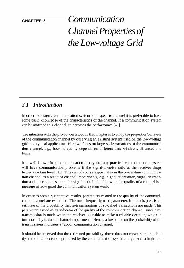
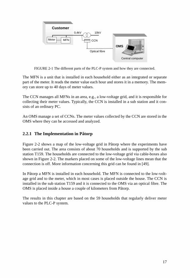
Figure 2-2 shows a map of the low-voltage grid in Påtorp where the experiments havebeen carried out. The area consists of about 70 households and is supported by the substation T159. The households are connected to the low-voltage grid via cable-boxes alsoshown in Figure 2-2. The markers placed on some of the low-voltage lines mean that theconnection is off. More information concerning this grid can be found in [49].

In Påtorp a MFN is installed in each household. The MFN is connected to the low-volt-age grid and to the meter, which in most cases is placed outside the house. The CCN isinstalled in the sub station T159 and it is connected to the OMS via an optical fibre. TheOMS is placed inside a house a couple of kilometers from Påtorp.

The results in this chapter are based on the 59 households that regularly deliver metervalues to the PLC-P system.

Optical fibre

Meter

Customer

CCN

OMS

Central computer

MFN

0,4kV 10kV

18

FIGURE 2-2 The low-voltage grid in Påtorp. The numbers are related to the cable-boxes (shown with black rectangles) and the sub station is denoted T159.

2.2.2 The Communication in PLC-P

The communication between the CCN and the MFNs is in all cases over the power-line.Every hour the CCN polls each MFN in order to get the meter values. To control theMFNs, and to read the meter values, a series of transactions are needed. A transaction isdefined as the combined sequence of a request by the CCN followed by a reply, withsome data, from a MFN. For every transaction, the communication system, on whichPLC-P is built (see Section 2.2.3), is invoked. If a transaction fails then PLC-P is notifiedand the CCN tries again until the transaction is succeeded. All communication isbetween the CCN and the MFNs. There is no communication between the households inthe area.

The result of each transaction, whether it has failed or not, is noted in a logfile for furtherprocessing. This logfile can be used to retrieve information about the communicationperformance. The information that has been used in this paper is the following:

ei, the number of failed transactions to household i

Ni, the total number of transactions to household i

New values are obtained each hour. If the communication is error-free, Ni is typically

two per hour and ei is zero per hour.

cable-box

sub station

19

All estimated results related to communication channel properties in this chapter havebeen calculated with the parameters above.

The collected meter values are stored in a file in the OMS. These values have been usedto study the effect of the loads on the channel quality, see Section 2.5.

2.2.3 The Communication Technique

PLC-P communicates in the frequency band 9-95 kHz. This is the frequency bandwidthset up by the CENELEC standard [8] exclusively for utilities, the so-called A Band. Thebit rate is low, a few kb/s, and the communication technique used is spread-spectrum[41] based.

2.3 Estimated Overall Performance of the Communication Channels

In Påtorp the CCN communicates with 59 MFNs, which are geographically spread.Hence, this means that 59 communication channels are present in the area, and the qual-ity of these channels can be very different. In this section, the overall (average) perfor-mance of these communication channels is estimated and discussed.

With the information given in the logfiles, an estimate, Pi, of the probability for re-trans-

mission of a transaction between the CCN and household number i (MFN number i), canbe obtained as:

(2-1)

This parameter is an estimate of the probability of rejection of an individual transactionat the CCN due to channel impairments, but we prefer to refer to Pi as an estimated chan-

nel impairment indicator to household i.

To be able to follow how the quality of the communication channels changes over time(large-scale variations), new estimates are calculated for each hour (normally). Thoughthe available statistical data is limited, the obtained quantitative results can be used as anindication of how the quality of the communication channels depends on different time-windows, distances and loads.

2.3.1 The Average Performance of the Channels

The average, P, of the channel impairment indicators, Pi, is a measure of the overall aver-age quality of the K (=59) communication channels in the area during an hour and isobtained as:

Pi=ei

Ni-----

20

(2-2)

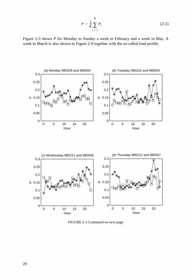
Figure 2-3 shows P for Monday to Sunday a week in February and a week in May. Aweek in March is also shown in Figure 2-9 together with the so-called load profile.

FIGURE 2-3 Continued on next page

P1K---- Pi

i 1=

K

∑=

0 5 10 15 200

0.05

0.1

0.15

0.2

0.25

0.3

Hour

P

(a) Monday 980209 and 980504

0 5 10 15 200

0.05

0.1

0.15

0.2

0.25

0.3

Hour

P

(b) Tuesday 980210 and 980505

0 5 10 15 200

0.05

0.1

0.15

0.2

0.25

0.3

Hour

P

(c) Wednesday 980211 and 980506

0 5 10 15 200

0.05

0.1

0.15

0.2

0.25

0.3

Hour

P

(d) Thursday 980212 and 980507

21

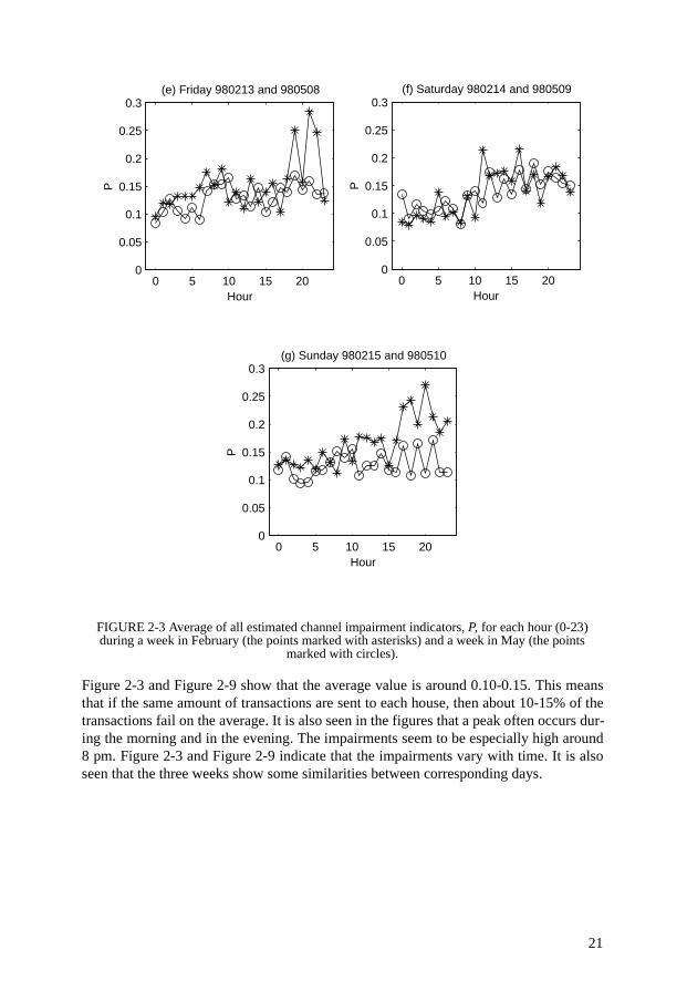
FIGURE 2-3 Average of all estimated channel impairment indicators, P, for each hour (0-23) during a week in February (the points marked with asterisks) and a week in May (the points

marked with circles).

Figure 2-3 and Figure 2-9 show that the average value is around 0.10-0.15. This meansthat if the same amount of transactions are sent to each house, then about 10-15% of thetransactions fail on the average. It is also seen in the figures that a peak often occurs dur-ing the morning and in the evening. The impairments seem to be especially high around8 pm. Figure 2-3 and Figure 2-9 indicate that the impairments vary with time. It is alsoseen that the three weeks show some similarities between corresponding days.

0 5 10 15 200

0.05

0.1

0.15

0.2

0.25

0.3

Hour

P(e) Friday 980213 and 980508

0 5 10 15 200

0.05

0.1

0.15

0.2

0.25

0.3

Hour

P

(f) Saturday 980214 and 980509

0 5 10 15 200

0.05

0.1

0.15

0.2

0.25

0.3

Hour

P

(g) Sunday 980215 and 980510

22

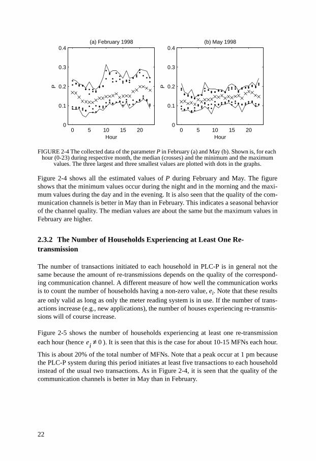
FIGURE 2-4 The collected data of the parameter P in February (a) and May (b). Shown is, for each hour (0-23) during respective month, the median (crosses) and the minimum and the maximum

values. The three largest and three smallest values are plotted with dots in the graphs.

Figure 2-4 shows all the estimated values of P during February and May. The figureshows that the minimum values occur during the night and in the morning and the maxi-mum values during the day and in the evening. It is also seen that the quality of the com-munication channels is better in May than in February. This indicates a seasonal behaviorof the channel quality. The median values are about the same but the maximum values inFebruary are higher.

2.3.2 The Number of Households Experiencing at Least One Re-transmission

The number of transactions initiated to each household in PLC-P is in general not thesame because the amount of re-transmissions depends on the quality of the correspond-ing communication channel. A different measure of how well the communication worksis to count the number of households having a non-zero value, ei. Note that these resultsare only valid as long as only the meter reading system is in use. If the number of trans-actions increase (e.g., new applications), the number of houses experiencing re-transmis-sions will of course increase.

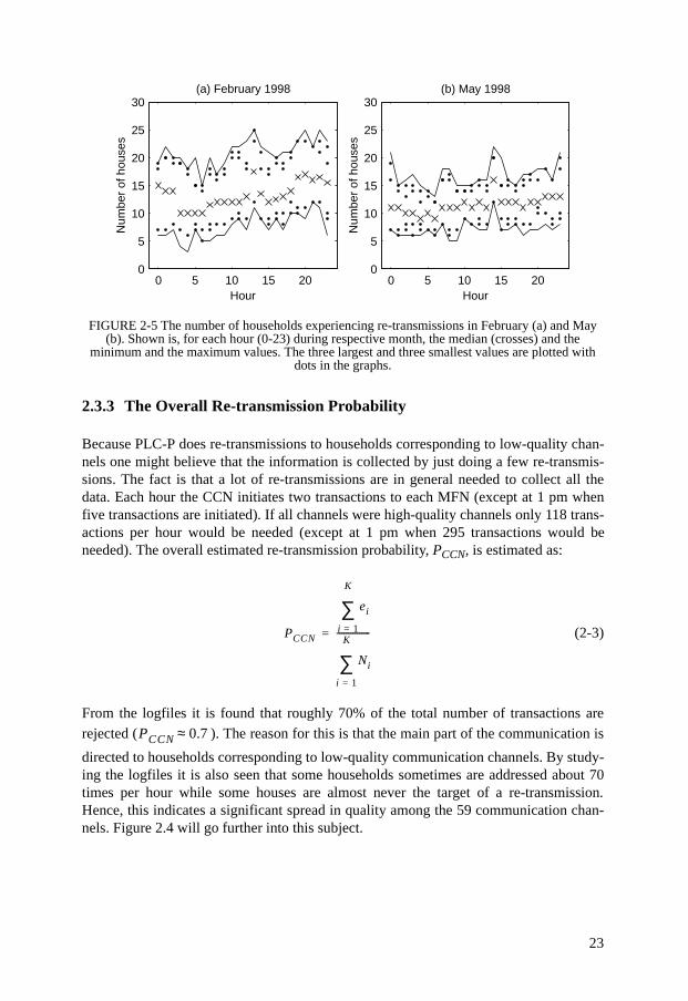
Figure 2-5 shows the number of households experiencing at least one re-transmissioneach hour (hence ). It is seen that this is the case for about 10-15 MFNs each hour.

This is about 20% of the total number of MFNs. Note that a peak occur at 1 pm becausethe PLC-P system during this period initiates at least five transactions to each householdinstead of the usual two transactions. As in Figure 2-4, it is seen that the quality of thecommunication channels is better in May than in February.

0 5 10 15 200

0.1

0.2

0.3

0.4

Hour

P

(a) February 1998

0 5 10 15 200

0.1

0.2

0.3

0.4

Hour

P

(b) May 1998

ei 0≠

23

FIGURE 2-5 The number of households experiencing re-transmissions in February (a) and May (b). Shown is, for each hour (0-23) during respective month, the median (crosses) and the

minimum and the maximum values. The three largest and three smallest values are plotted with dots in the graphs.

2.3.3 The Overall Re-transmission Probability

Because PLC-P does re-transmissions to households corresponding to low-quality chan-nels one might believe that the information is collected by just doing a few re-transmis-sions. The fact is that a lot of re-transmissions are in general needed to collect all thedata. Each hour the CCN initiates two transactions to each MFN (except at 1 pm whenfive transactions are initiated). If all channels were high-quality channels only 118 trans-actions per hour would be needed (except at 1 pm when 295 transactions would beneeded). The overall estimated re-transmission probability, PCCN, is estimated as:

(2-3)

From the logfiles it is found that roughly 70% of the total number of transactions arerejected ( ). The reason for this is that the main part of the communication is

directed to households corresponding to low-quality communication channels. By study-ing the logfiles it is also seen that some households sometimes are addressed about 70times per hour while some houses are almost never the target of a re-transmission.Hence, this indicates a significant spread in quality among the 59 communication chan-nels. Figure 2.4 will go further into this subject.

0 5 10 15 200

5

10

15

20

25

30

Hour

Num

ber

of h

ouse

s

(a) February 1998

0 5 10 15 200

5

10

15

20

25

30

Hour

Num

ber

of h

ouse

s

(b) May 1998

PCCN

ei

i 1=

K

∑

Ni

i 1=

K

∑

---------------=

PCCN 0.7≈

24

2.4 Channel Performance Associated with Specific Cable-Boxes in the Grid

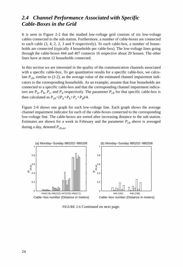
It is seen in Figure 2-2 that the studied low-voltage grid consists of six low-voltagecables connected to the sub station. Furthermore, a number of cable-boxes are connectedto each cable (3, 4, 2, 2, 3 and 9 respectively). To each cable-box, a number of house-holds are connected (typically 4 households per cable-box). The low-voltage lines goingthrough the cable-boxes 444 and 407 connects 16 respective about 20 houses. The otherlines have at most 12 households connected.

In this section we are interested in the quality of the communication channels associatedwith a specific cable-box. To get quantitative results for a specific cable-box, we calcu-late Pcb, similar to (2-2), as the average value of the estimated channel impairment indi-

cators to the corresponding households. As an example; assume that four households areconnected to a specific cable-box and that the corresponding channel impairment indica-tors are Pa, Pb, Pc, and Pd respectively. The parameter Pcb for that specific cable-box isthen calculated as Pcb=(Pa+Pb+Pc+Pd)/4.

Figure 2-6 shows one graph for each low-voltage line. Each graph shows the averagechannel impairment indicator for each of the cable-boxes connected to the correspondinglow-voltage line. The cable-boxes are sorted after increasing distance to the sub station.Estimates are shown for a week in February and the parameter Pcb above is averaged

during a day, denoted Pcb,av.

FIGURE 2-6 Continued on next page.

444(119) 445(152) 447(220) 446(271)0

0.2

0.4

0.6

0.8

1

Cable−box number (Distance in meters)

Pcb

,av

(a) Monday−Sunday 980202−980208

449 (162) 448 (198)0

0.2

0.4

0.6

0.8

1

Cable−box number (Distance in meters)

Pcb

,av

(b) Monday−Sunday 980202−980208

25

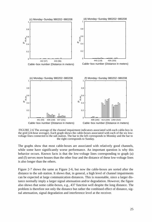
FIGURE 2-6 The average of the channel impairment indicators associated with each cable-box in the grid (24-hour average). Each graph shows the cable-boxes associated with each of the six low-voltage lines connected to the sub station. The bar to the left corresponds to Monday and the bar to

the right corresponds to Sunday.

The graphs show that most cable-boxes are associated with relatively good channels,while some have significantly worse performance. An important question is why thisbehavior occurs. Known facts is that the low-voltage lines corresponding to graph (a)and (f) serves more houses than the other four and the distance of these low-voltage linesis also longer than the others.

Figure 2-7 shows the same as Figure 2-6, but now the cable-boxes are sorted after thedistance to the sub station. It shows that, in general, a high level of channel impairmentscan be expected at large communication distances. This is reasonable, since a larger dis-tance normally imply a larger signal attenuation and/or degradation. However, the figurealso shows that some cable-boxes, e.g., 437 function well despite the long distance. Theproblem is therefore not only the distance but rather the combined effect of distance, sig-nal attenuation, signal degradation and interference level at the receiver.

442 (57) 443 (96)0

0.2

0.4

0.6

0.8

1

Cable−box number (Distance in meters)

Pcb

,av

(c) Monday−Sunday 980202−980208

440 (118) 439 (183)0

0.2

0.4

0.6

0.8

1

Cable−box number (Distance in meters)

Pcb

,av

(d) Monday−Sunday 980202−980208

441 (93) 438 (158) 437 (231)0

0.2

0.4

0.6

0.8

1

Cable−box number (Distance in meters)

Pcb

,av

(e) Monday−Sunday 980202−980208

408 (165) 413 (230) 1350 (310)0

0.2

0.4

0.6

0.8

1

Cable−box number (Distance in meters)

Pcb

,av

(f) Monday−Sunday 980202−980208

26

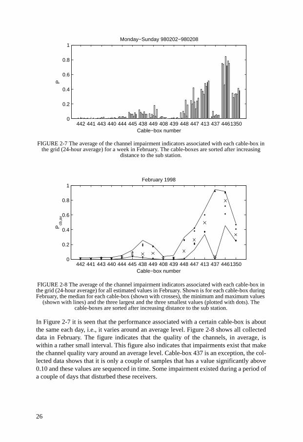
FIGURE 2-7 The average of the channel impairment indicators associated with each cable-box in the grid (24-hour average) for a week in February. The cable-boxes are sorted after increasing

distance to the sub station.

FIGURE 2-8 The average of the channel impairment indicators associated with each cable-box in the grid (24-hour average) for all estimated values in February. Shown is for each cable-box during February, the median for each cable-box (shown with crosses), the minimum and maximum values

(shown with lines) and the three largest and the three smallest values (plotted with dots). The cable-boxes are sorted after increasing distance to the sub station.

In Figure 2-7 it is seen that the performance associated with a certain cable-box is aboutthe same each day, i.e., it varies around an average level. Figure 2-8 shows all collecteddata in February. The figure indicates that the quality of the channels, in average, iswithin a rather small interval. This figure also indicates that impairments exist that makethe channel quality vary around an average level. Cable-box 437 is an exception, the col-lected data shows that it is only a couple of samples that has a value significantly above0.10 and these values are sequenced in time. Some impairment existed during a period ofa couple of days that disturbed these receivers.

442 441 443 440 444 445 438 449 408 439 448 447 413 437 44613500

0.2

0.4

0.6

0.8

1

Cable−box number

P

Monday−Sunday 980202−980208

442 441 443 440 444 445 438 449 408 439 448 447 413 437 44613500

0.2

0.4

0.6

0.8

1

Cable−box number

Pcb

,av

February 1998

27

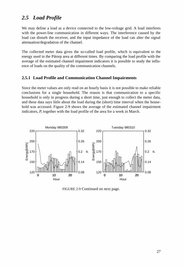
2.5 Load Profile

We may define a load as a device connected to the low-voltage grid. A load interfereswith the power-line communication in different ways. The interference caused by theload can disturb the receiver, and the input impedance of the load can alter the signalattenuation/degradation of the channel.

The collected meter data gives the so-called load profile, which is equivalent to theenergy used in the Påtorp area at different times. By comparing the load profile with theaverage of the estimated channel impairment indicators it is possible to study the influ-ence of loads on the quality of the communication channels.

2.5.1 Load Profile and Communication Channel Impairments

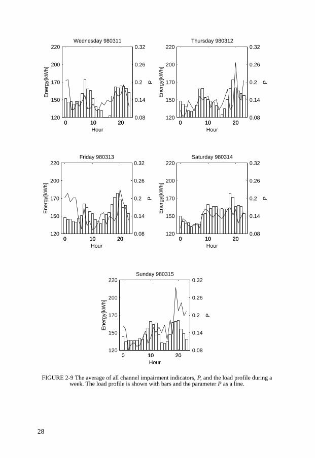
Since the meter values are only read on an hourly basis it is not possible to make reliableconclusions for a single household. The reason is that communication to a specifichousehold is only in progress during a short time, just enough to collect the meter data,and these data says little about the load during the (short) time interval when the house-hold was accessed. Figure 2-9 shows the average of the estimated channel impairmentindicators, P, together with the load profile of the area for a week in March.

FIGURE 2-9 Continued on next page.

0 10 20120

150

170

200

220

Ene

rgy[

kWh]

0 10 200.08

0.14

0.2

0.26

0.32

P

Monday 980309

Hour0 10 20

120

150

170

200

220

Ene

rgy[

kWh]

0 10 200.08

0.14

0.2

0.26

0.32

P

Tuesday 980310

Hour

28

FIGURE 2-9 The average of all channel impairment indicators, P, and the load profile during a week. The load profile is shown with bars and the parameter P as a line.

0 10 20120

150

170

200

220E

nerg

y[kW

h]

0 10 200.08

0.14

0.2

0.26

0.32

P

Wednesday 980311

Hour0 10 20

120

150

170

200

220

Ene

rgy[

kWh]

0 10 200.08

0.14

0.2

0.26

0.32

P

Thursday 980312

Hour

0 10 20120

150

170

200

220

Ene

rgy[

kWh]

0 10 200.08

0.14

0.2

0.26

0.32

P

Friday 980313

Hour0 10 20

120

150

170

200

220E

nerg

y[kW

h]

0 10 200.08

0.14

0.2

0.26

0.32

P

Saturday 980314

Hour

0 10 20120

150

170

200

220

Ene

rgy[

kWh]

0 10 200.08

0.14

0.2

0.26

0.32

P

Sunday 980315

Hour

29

The figure shows that peaks in the load profile occur in the morning and in the evening.During the weekend the morning peak is delayed. The behavior shown is typical in alow-voltage grid consisting of only households.

It is also seen that in many cases when the energy usage is high the quality of the com-munication channels is low (the channel impairment indicators are high). This is asexpected because when the energy usage is high, more devices are connected to the gridand hence more possible sources of impairments exist.

The relation between the two parameters is not linear because the dependence betweenthe energy usage of a device and its impairment on the channel is not linear. Thereforethe quality of the channels can be low even though the energy usage is low.

2.6 Conclusions

In this chapter, focus is on the quality of the communication channels in a specific low-voltage grid. By processing collected data, obtained from a running meter reading sys-tem (PLC-P) operating in the low-voltage grid, estimates of channel impairment parame-ters are obtained. Hence, the PLC-P system is not evaluated here, rather it is used toextract information that can be used for (large-scale) channel quality estimation. Thisstudy is based on collected data representing communication with 59 households (hence,59 communication channels are considered), and the low-voltage grid is located in Ron-neby, Sweden.

The overall average quality of the communication channels fluctuates more or less ran-domly for each hour within a day, and also for each day within a week. However, theaverage quality seems to vary around a level that corresponds to a re-transmission proba-bility roughly equal to 0.15. By comparing the results for February and for May, it is seenthat less variations are obtained for May, which indicates a seasonal behavior of thechannel quality.

Large variations in the quality between the individual communication channels have alsobeen found. Especially, for the considered low-voltage grid, low-quality communicationchannels have been found along two, of the six, lines leaving the transformer. A low-quality communication channel is normally the result of the combined effect of channelimpairments such as signal attenuation, signal degradation and interference level at thereceiver. However, based on the collected data, we are not able to decide which is thedominating impairment. From the results it is also seen that there is a clear tendency thatthe quality of a specific communication channel varies randomly around an "averagequality level", which in turn depends on the path of the channel in the grid.

It is well-known that re-transmission methods can be used where real-time operation isnot a critical issue and where the information bit rate is low (e.g., meter reading sys-tems). A consequence of low-quality communication channels is that the main part of thecommunication is over these channels, since many re-transmissions are in general neces-sary to obtain reliability. The PLC-P system is designed for collecting meter values and it

30

uses a re-transmission method for this purpose. Hence, it takes some time until all the 59meter values are collected. However, this time-delay is not critical in the current applica-tion.

The loads connected to the low-voltage grid can have a serious impact on the communi-cation performance. In general a load can introduce several effects; it can, e.g., changethe attenuation and/or the degradation of the information-carrying signals. Furthermore,a load can also introduce interfering signals. A general problem is that the set of activeloads in a given time interval is random. Despite these difficulties it is interesting tostudy the level of channel impairments in relation to the amount of energy delivered tothe grid (the so-called load profile). From the observed data it is hard to draw any defini-tive conclusions. However, a period of high energy consumption (typically mornings andevenings) in the grid have a tendency to decrease the channel quality. It is also observedthat the quality of the channels can be low at nights, though the energy consumption islow. An explanation might be that the loads in this case generate severe interfering sig-nals. To further explore the effect of loads in power-line communications a load designedfor test purposes was moved to Påtorp. The impact of this specific load is described inthe following chapter.

The investigations reported in this chapter can be characterized as an attempt to get anoverview of some communication channel properties of the low-voltage grid. Thoughadditional specific (small-scale) measurements have to be made, it is already clear thatadvanced communication methods must be used in forthcoming applications requiringhigh information bit rates. Key parameters are the available bandwidth and the corre-sponding signal-to noise ratio at the receiver. Several well-known communication meth-ods are possible candidates for future use in power-line applications. Examples areOFDM-type methods [18], GMSK-type methods [33], and methods based on spread-spectrum techniques [41]. For a given application, parameters that will influence thechoice of communication method are; the characteristics of the communication channelwithin the communication bandwidth, the required information bit rate, real-timedemands and the required level of robustness.

31

CHAPTER 3 On the Effect of Loads on Power-Line Communications

3.1 Introduction

In the previous chapter we have studied some properties of specific channels in a specificlow-voltage grid. As Section 2.5 indicates, the various loads connected to the power-linecan decrease the quality of the communication channels. However, based on the col-lected data it can not be said how strong this influence is. To investigate this further amoveable load has been transported to the grid in Påtorp (for a description of this gridsee Section 2.2.1). This load is designed by NESA A/S (a utility distributor in Denmark)and it consists of a set of industrial machines mounted within a container.

More specifically, the moveable load consists of a 65 kVA voltage source inverter, whichdrives a 40 kW induction motor, which drives a 48 kVA synchronous generator, supply-ing power to some 45 kW heaters. Inside the container there is also a 35 kVA weldingunit. The energy usage of the load when all devices are active is roughly 68 kWh perhour. This can be compared with the total energy usage per hour shown in Figure 2-9.

The moveable load was connected to various places in the low-voltage grid in order toinvestigate how it affected the quality of the communication channels. It was placed inthe sub station to see how it affected all channels, and in cable-boxes to see the influenceon specific communication channels. Because the PLC-P system (see Section 2.2) usesone hour to access all households it was necessary to let the load be on during at least anentire hour without interruption. The results of these experiments are shown in Section3.2.

An objective with these experiments has also been to measure the harmonic disturbancesintroduced in the grid by the load. The frequencies considered in this chapter are har-monics (of the 50 Hz mains signaling voltage) up to 2.5 kHz. This is described in Section3.3.

32

3.2 The Influence of the Load on the Communication

3.2.1 The Influence of the Load when Connected to the Sub Station

The moveable load was first connected to the sub station, see Figure 2-2. By doing this itwas made sure that the load influenced every message sent (received) from (at) the CCN.

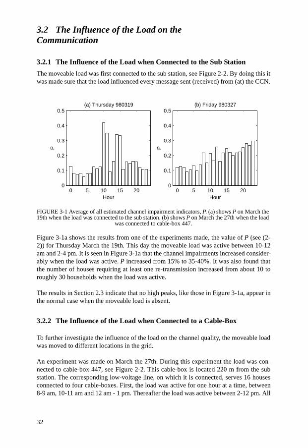
FIGURE 3-1 Average of all estimated channel impairment indicators, P. (a) shows P on March the 19th when the load was connected to the sub station. (b) shows P on March the 27th when the load

was connected to cable-box 447.

Figure 3-1a shows the results from one of the experiments made, the value of P (see (2-2)) for Thursday March the 19th. This day the moveable load was active between 10-12am and 2-4 pm. It is seen in Figure 3-1a that the channel impairments increased consider-ably when the load was active. P increased from 15% to 35-40%. It was also found thatthe number of houses requiring at least one re-transmission increased from about 10 toroughly 30 households when the load was active.

The results in Section 2.3 indicate that no high peaks, like those in Figure 3-1a, appear inthe normal case when the moveable load is absent.

3.2.2 The Influence of the Load when Connected to a Cable-Box

To further investigate the influence of the load on the channel quality, the moveable loadwas moved to different locations in the grid.

An experiment was made on March the 27th. During this experiment the load was con-nected to cable-box 447, see Figure 2-2. This cable-box is located 220 m from the substation. The corresponding low-voltage line, on which it is connected, serves 16 housesconnected to four cable-boxes. First, the load was active for one hour at a time, between8-9 am, 10-11 am and 12 am - 1 pm. Thereafter the load was active between 2-12 pm. All

0 5 10 15 200

0.1

0.2

0.3

0.4

0.5

Hour

P

(a) Thursday 980319

0 5 10 15 200

0.1

0.2

0.3

0.4

0.5

Hour

P

(b) Friday 980327

33

the machines were used during the whole experiment except the welding unit, whichonly was on between 10-11 am, 12 am - 1 pm and 2-3 pm.

Figure 3-1b shows the value of P (see (2-2)) for March the 27th. This figure shows thatat this location the moveable load did not degrade the channel quality as much as when itwas located at the sub station. The average of the channel impairment indicatorsincreased from 15% to 20-25%. One reason is the long distance between the load and thesub station. Hence, not so many communication channels are affected by the load. Only25% of the households are connected to this low-voltage line so assuming the load doesnot cause too much interference in the other low-voltage lines the value of P should belower.

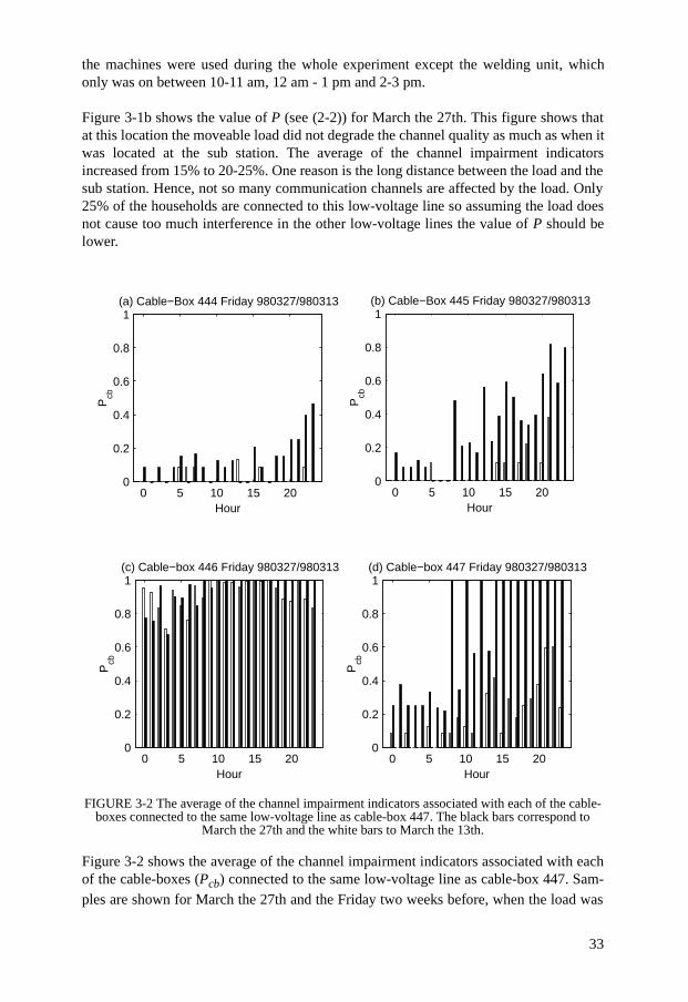
FIGURE 3-2 The average of the channel impairment indicators associated with each of the cable-boxes connected to the same low-voltage line as cable-box 447. The black bars correspond to

March the 27th and the white bars to March the 13th.

Figure 3-2 shows the average of the channel impairment indicators associated with eachof the cable-boxes (Pcb) connected to the same low-voltage line as cable-box 447. Sam-ples are shown for March the 27th and the Friday two weeks before, when the load was

0 5 10 15 200

0.2

0.4

0.6

0.8

1

Hour

Pcb

(a) Cable−Box 444 Friday 980327/980313

0 5 10 15 200

0.2

0.4

0.6

0.8

1

Hour

Pcb

(b) Cable−Box 445 Friday 980327/980313

0 5 10 15 200

0.2

0.4

0.6

0.8

1

Hour

Pcb

(c) Cable−box 446 Friday 980327/980313

0 5 10 15 200

0.2

0.4

0.6

0.8

1

Hour

Pcb

(d) Cable−box 447 Friday 980327/980313

34

not connected. The figure indicates that when the load was active a severe degradation ofchannel quality occurred to households connected to the cable-box where the load wasconnected.

Cable-box 446 is placed on a longer distance to the sub station than cable-box 447 andrepresents a low-quality channel. As Figure 3-2 shows, this cable-box was a low-qualitychannel even when the load was not connected. The channels associated with the cable-boxes located closer to the sub station were also effected by the load. Peaks are shownfor cable-box 445 at times when the load was active. A study of cable-boxes 442 and443, which belong to another low-voltage line, shows that they are very little affected.

Even when the load was not active one heater was on warming the container. This canexplain why Pcb seems to be higher even when the load is not active.

3.3 Measurements of the Harmonic Voltages and Currents Introduced by the Load

In order to show the harmonic disturbance introduced in the grid by the load, harmonicvoltages and currents have been measured at various locations in the grid. The measure-ments have been carried out with an Oscillostore P513 [50] from Siemens and a Scop-Meter F99 [19] from Fluke. P513 is capable of measuring, e.g., voltage, current, powerand harmonics (up to 2.5 kHz), has 12-bit resolution and a sample frequency of 12.8kHz. F99 is a handheld 50 MHz oscilloscope with a vertical resolution of 8 bits and canmeasure THD (Total Harmonic Distorsion) [9].

The load is considered a three-phase unit but measurements show that the current drawnfrom the welding unit is asymmetrical. The highest average harmonic currents are drawnfrom phase two and this phase is used as a reference in this section. Test measurementshave also shown that the highest harmonic voltages and currents of the load is located inthe odd harmonics between 3 and 19. Therefore only the odd harmonics from 3 to 19have been measured (the reason is also because of the limited storage capacity in themeasurement device).

The measurements presented in the rest of this section are from the same experiment asdescribed in Section 3.2.2. During this experiment the load was connected to cable-box447, see Figure 2-2. First, the load was active for one hour at a time, between 8-9 am, 10-11 am and 12 am - 1 pm. Thereafter the load was active between 2-12 pm. In this section,only the time interval between 8 am and 15 pm is considered. All the machines wereused during the whole experiment (considered in this section) except the welding unit,which was not on in the first time interval.

Note that the PLC-P system (at the time of trials) was 15 minutes before real time, there-fore the measurements have been started 15 minutes earlier to comply with the time inPLC-P.

35

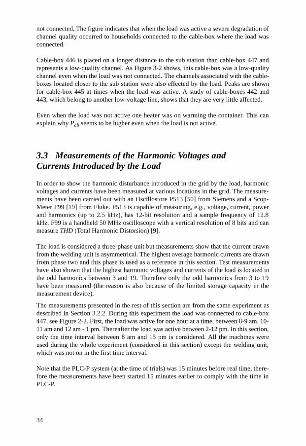
3.3.1 The Harmonic Disturbance Introduced in the Grid

Figure 3-3 shows the measured fundamental current and the odd harmonics (for ordersup to seven) drawn by the load in the considered time interval. The current change whenthe welding unit was in use is approximately 20 A. This arose because the welding elec-trode had to be replaced each time it was used up.

FIGURE 3-3 The measured fundamental current and the odd harmonic currents (for orders up to seven) drawn by the load. The x-axis shows time and the y-axis the current in Ampere.

The maximum amplitude for the fundamental current and the odd harmonic currents (fororders up to 19) in the time interval 8 am - 15 pm are shown in Figure 3-4.

0

1 0

2 0

3 0

4 0

5 0

6 0

0 7 : 4 5 0 8 : 5 7 1 0 : 0 9 1 1 : 2 1 1 2 : 3 3 1 3 : 4 5

1. h

arm

. L2

[A]

0

1 0

2 0

3 0

4 0

5 0

6 0

0 7 : 4 5 0 8 : 5 7 1 0 : 0 9 1 1 : 2 1 1 2 : 3 3 1 3 : 4 5

3. h

arm

. L2

[A

]

0

1 0

2 0

3 0

4 0

5 0

6 0

0 7 : 4 5 0 8 : 5 7 1 0 : 0 9 1 1 : 2 1 1 2 : 3 3 1 3 : 4 5

5. h

arm

. L2

[A

]

0

1 0

2 0

3 0

4 0

5 0

6 0

0 7 : 4 5 0 8 : 5 7 1 0 : 0 9 1 1 : 2 1 1 2 : 3 3 1 3 : 4 5h h : m m

7. h

arm

. L2

[A]

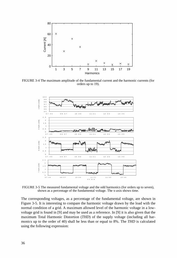
36

FIGURE 3-4 The maximum amplitude of the fundamental current and the harmonic currents (for orders up to 19).

FIGURE 3-5 The measured fundamental voltage and the odd harmonics (for orders up to seven), shown as a percentage of the fundamental voltage. The x-axis shows time.

The corresponding voltages, as a percentage of the fundamental voltage, are shown inFigure 3-5. It is interesting to compare the harmonic voltage drawn by the load with thenormal condition of a grid. A maximum allowed level of the harmonic voltage in a low-voltage grid is found in [9] and may be used as a reference. In [9] it is also given that themaximum Total Harmonic Distortion (THD) of the supply voltage (including all har-monics up to the order of 40) shall be less than or equal to 8%. The THD is calculatedusing the following expression:

1 3 5 7 9 11 13 15 17 190

20

40

60

80

Harmonics

Cur

rent

[A]

9 4

9 5

9 6

9 7

9 8

9 9

1 0 0

0 7 : 4 5 0 8 : 5 7 1 0 : 0 9 1 1 : 2 1 1 2 : 3 3 1 3 : 4 5

1. h

arm

. L2

[%]

0

0 , 5

1

1 , 5

2

2 , 5

0 7 : 4 5 0 8 : 5 7 1 0 : 0 9 1 1 : 2 1 1 2 : 3 3 1 3 : 4 5

3. h

arm

. L2

[%]

0

0 , 5

1

1 , 5

2

2 , 5

0 7 : 4 5 0 8 : 5 7 1 0 : 0 9 1 1 : 2 1 1 2 : 3 3 1 3 : 4 5

5. h

arm

. L2

[%]

0

0 , 5

1

1 , 5

2

2 , 5

0 7 : 4 5 0 8 : 5 7 1 0 : 0 9 1 1 : 2 1 1 2 : 3 3 1 3 : 4 5

h h : m m

7.

ha

rm.

L2 [

%]

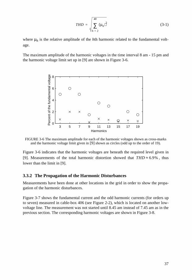
37

(3-1)

where µh is the relative amplitude of the hth harmonic related to the fundamental volt-

age.

The maximum amplitude of the harmonic voltages in the time interval 8 am - 15 pm andthe harmonic voltage limit set up in [9] are shown in Figure 3-6.

FIGURE 3-6 The maximum amplitude for each of the harmonic voltages shown as cross-marks and the harmonic voltage limit given in [9] shown as circles (odd up to the order of 19).

Figure 3-6 indicates that the harmonic voltages are beneath the required level given in[9]. Measurements of the total harmonic distortion showed that , thuslower than the limit in [9].

3.3.2 The Propagation of the Harmonic Disturbances

Measurements have been done at other locations in the grid in order to show the propa-gation of the harmonic disturbances.

Figure 3-7 shows the fundamental current and the odd harmonic currents (for orders upto seven) measured in cable-box 406 (see Figure 2-2), which is located on another low-voltage line. The measurement was not started until 8.45 am instead of 7.45 am as in theprevious section. The corresponding harmonic voltages are shown in Figure 3-8.

THD µh( )2

h 2=

40

∑=

3 5 7 9 11 13 15 17 190

2

4

6

8

Harmonics

Per

cent

of t

he fu

ndam

enta

l vol

tage

THD 6.9%≈

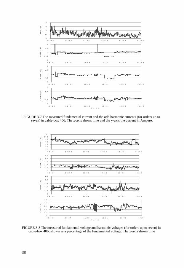
38

FIGURE 3-7 The measured fundamental current and the odd harmonic currents (for orders up to seven) in cable-box 406. The x-axis shows time and the y-axis the current in Ampere.

FIGURE 3-8 The measured fundamental voltage and harmonic voltages (for orders up to seven) in cable-box 406, shown as a percentage of the fundamental voltage. The x-axis shows time

0

1 0

2 0

3 0

4 0

0 8 : 4 5 0 9 : 5 7 1 1 : 0 9 1 2 : 2 1 1 3 : 3 3 1 4 : 4 51.

ha

rm.

L2 [A

]

0

0 , 5

1

1 , 5

2

0 8 : 4 5 0 9 : 5 7 1 1 : 0 9 1 2 : 2 1 1 3 : 3 3 1 4 : 4 5

3. h

arm

. L2

[A

]

0

0 , 5

1

1 , 5

2

0 8 : 4 5 0 9 : 5 7 1 1 : 0 9 1 2 : 2 1 1 3 : 3 3 1 4 : 4 5

5. h

arm

. L2

[A

]

0

0 , 5

1

1 , 5

2

0 8 : 4 5 0 9 : 5 7 1 1 : 0 9 1 2 : 2 1 1 3 : 3 3 1 4 : 4 5h h : m m

7. h

arm

. L2

[A]

9 5

9 6

9 7

9 8

9 9

1 0 0

1 0 1

0 8 : 4 5 0 9 : 5 7 1 1 : 0 9 1 2 : 2 1 1 3 : 3 3 1 4 : 4 5

1. h

arm

. L2

[%]

0

0 , 3

0 , 6

0 , 9

1 , 2

1 , 5

0 8 : 4 5 0 9 : 5 7 1 1 : 0 9 1 2 : 2 1 1 3 : 3 3 1 4 : 4 5

3. h

arm

. L2

[%]

0

0 , 3

0 , 6

0 , 9

1 , 2

1 , 5

0 8 : 4 5 0 9 : 5 7 1 1 : 0 9 1 2 : 2 1 1 3 : 3 3 1 4 : 4 5

5. h

arm

. L2

[%]

0

0 , 3

0 , 6

0 , 9

1 , 2

1 , 5

0 8 : 4 5 0 9 : 5 7 1 1 : 0 9 1 2 : 2 1 1 3 : 3 3 1 4 : 4 5

h h : m m

7.

ha

rm.

L2 [

%]

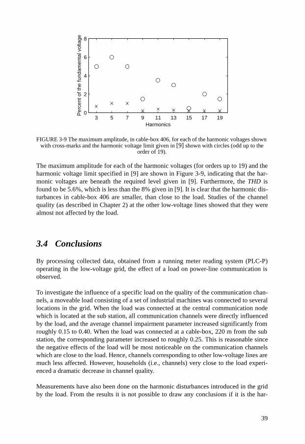
39

FIGURE 3-9 The maximum amplitude, in cable-box 406, for each of the harmonic voltages shown with cross-marks and the harmonic voltage limit given in [9] shown with circles (odd up to the

order of 19).

The maximum amplitude for each of the harmonic voltages (for orders up to 19) and theharmonic voltage limit specified in [9] are shown in Figure 3-9, indicating that the har-monic voltages are beneath the required level given in [9]. Furthermore, the THD isfound to be 5.6%, which is less than the 8% given in [9]. It is clear that the harmonic dis-turbances in cable-box 406 are smaller, than close to the load. Studies of the channelquality (as described in Chapter 2) at the other low-voltage lines showed that they werealmost not affected by the load.

3.4 Conclusions

By processing collected data, obtained from a running meter reading system (PLC-P)operating in the low-voltage grid, the effect of a load on power-line communication isobserved.

To investigate the influence of a specific load on the quality of the communication chan-nels, a moveable load consisting of a set of industrial machines was connected to severallocations in the grid. When the load was connected at the central communication nodewhich is located at the sub station, all communication channels were directly influencedby the load, and the average channel impairment parameter increased significantly fromroughly 0.15 to 0.40. When the load was connected at a cable-box, 220 m from the substation, the corresponding parameter increased to roughly 0.25. This is reasonable sincethe negative effects of the load will be most noticeable on the communication channelswhich are close to the load. Hence, channels corresponding to other low-voltage lines aremuch less affected. However, households (i.e., channels) very close to the load experi-enced a dramatic decrease in channel quality.

Measurements have also been done on the harmonic disturbances introduced in the gridby the load. From the results it is not possible to draw any conclusions if it is the har-

3 5 7 9 11 13 15 17 190

2

4

6

8

Harmonics

Per

cent

of t

he fu

ndam

enta

l vol

tage

40

monic disturbances that interrupts the communication or if it is the result of impairmentsin higher frequency bands. Measurements indicate that the injected harmonic voltage islower than the limit in [9]. This means that the load source can not be referred to as anabnormal condition of a grid.

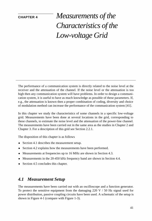
41

CHAPTER 4 Measurements of the Characteristics of the Low-voltage Grid

The performance of a communication system is directly related to the noise level at thereceiver and the attenuation of the channel. If the noise level or the attenuation is toohigh then any communication system will have problems. In order to design a communi-cation system, it is useful to have as much knowledge as possible of these parameters. If,e.g., the attenuation is known then a proper combination of coding, diversity and choiceof modulation method can increase the performance of the communication system [41].

In this chapter we study the characteristics of some channels in a specific low-voltagegrid. Measurements have been done at several locations in the grid, corresponding tothese channels, to estimate the noise level and the attenuation of the power-line channel.The measurements have been carried out in the same area as the studies in Chapter 2 andChapter 3. For a description of this grid see Section 2.2.1.

The disposition of this chapter is as follows

• Section 4.1 describes the measurement setup.

• Section 4.2 explains how the measurements have been performed.

• Measurements at frequencies up to 16 MHz are shown in Section 4.3.

• Measurements in the 20-450 kHz frequency band are shown in Section 4.4.

• Section 4.5 concludes this chapter.

4.1 Measurement Setup

The measurements have been carried out with an oscilloscope and a function generator.To protect the sensitive equipment from the damaging 220 V / 50 Hz signal used forpower distribution, passive coupling circuits have been used. A schematic of the setup isshown in Figure 4-1 (compare with Figure 1-3).

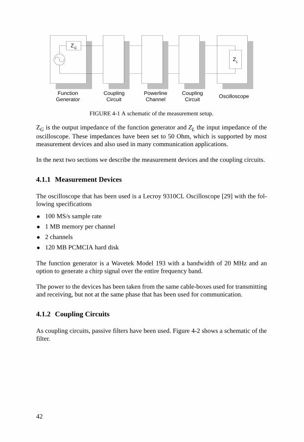
42

FIGURE 4-1 A schematic of the measurement setup.

ZG is the output impedance of the function generator and ZL the input impedance of theoscilloscope. These impedances have been set to 50 Ohm, which is supported by mostmeasurement devices and also used in many communication applications.

In the next two sections we describe the measurement devices and the coupling circuits.

4.1.1 Measurement Devices

The oscilloscope that has been used is a Lecroy 9310CL Oscilloscope [29] with the fol-lowing specifications

• 100 MS/s sample rate

• 1 MB memory per channel

• 2 channels

• 120 MB PCMCIA hard disk

The function generator is a Wavetek Model 193 with a bandwidth of 20 MHz and anoption to generate a chirp signal over the entire frequency band.

The power to the devices has been taken from the same cable-boxes used for transmittingand receiving, but not at the same phase that has been used for communication.

4.1.2 Coupling Circuits

As coupling circuits, passive filters have been used. Figure 4-2 shows a schematic of thefilter.

FunctionGenerator

CouplingCircuit

CouplingCircuit

PowerlineChannel

Oscilloscope

ZG

ZL

43

FIGURE 4-2 The coupling filter used to connect the measurement devices to the power-line.

The filter is a transformer isolated, differential mode, coupling circuit, and isolates theconnected device from the power-line. The capacitor C1 and the self-inductance, L1, ofthe transformer, T1, form a series resonance circuit, a high pass filter to effectivelyremove the 50 Hz signal and its harmonics, but also other spectral components with lowfrequencies. The varistor serves as a surge protection unit, minimizing the effect of tran-sients. Capacitor C2 prevents the transformer from shorting out the DC offset of thetransmitter and has not been mounted when the filter has been used as a receiver. Adescription of how to design filters for the power-line is given in [17].

Two variations of this filter have been used, Filter A and Filter B, see Table 4-1. The cut-off frequency, specified in Table 4-1, is the frequency for which the transfer functionmagnitude is -3dB.

TABLE 4-1 Component specification for Filter A and Filter B.

The squared magnitude of the frequency response of Filter A and Filter B is shown inFigure 4-3.

Filter A Filter B

C1 0.68 µF 0.1 µF

C2 10 µF 10 µF

L1 3.9 mH 1 mH

Cutoff fre-quency

3 kHz 25 kHz

C1C2

Line

Varistor

Neutral

L1

T1

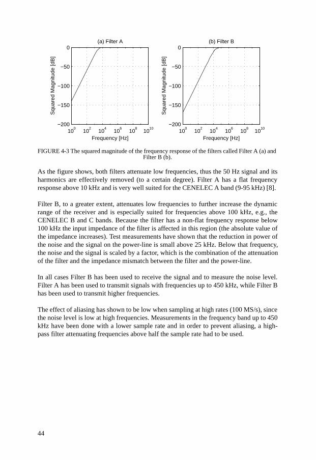
44

FIGURE 4-3 The squared magnitude of the frequency response of the filters called Filter A (a) and Filter B (b).

As the figure shows, both filters attenuate low frequencies, thus the 50 Hz signal and itsharmonics are effectively removed (to a certain degree). Filter A has a flat frequencyresponse above 10 kHz and is very well suited for the CENELEC A band (9-95 kHz) [8].

Filter B, to a greater extent, attenuates low frequencies to further increase the dynamicrange of the receiver and is especially suited for frequencies above 100 kHz, e.g., theCENELEC B and C bands. Because the filter has a non-flat frequency response below100 kHz the input impedance of the filter is affected in this region (the absolute value ofthe impedance increases). Test measurements have shown that the reduction in power ofthe noise and the signal on the power-line is small above 25 kHz. Below that frequency,the noise and the signal is scaled by a factor, which is the combination of the attenuationof the filter and the impedance mismatch between the filter and the power-line.

In all cases Filter B has been used to receive the signal and to measure the noise level.Filter A has been used to transmit signals with frequencies up to 450 kHz, while Filter Bhas been used to transmit higher frequencies.

The effect of aliasing has shown to be low when sampling at high rates (100 MS/s), sincethe noise level is low at high frequencies. Measurements in the frequency band up to 450kHz have been done with a lower sample rate and in order to prevent aliasing, a high-pass filter attenuating frequencies above half the sample rate had to be used.

100

102

104

106

108

1010

−200

−150

−100

−50

0

Frequency [Hz]

Squ

ared

Mag

nitu

de [d

B]

(a) Filter A

100

102

104

106

108

1010

−200

−150

−100

−50

0

Frequency [Hz]

Squ

ared

Mag

nitu

de [d

B]

(b) Filter B

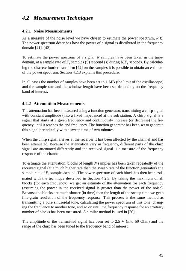
45

4.2 Measurement Techniques

4.2.1 Noise Measurements

As a measure of the noise level we have chosen to estimate the power spectrum, R(f).The power spectrum describes how the power of a signal is distributed in the frequencydomain [41], [42].

To estimate the power spectrum of a signal, N samples have been taken in the time-domain, at a sample rate of Fs samples (S) /second (s) during N/Fs seconds. By calculat-ing the discrete fourier transform [42] on the samples it is possible to obtain an estimateof the power spectrum. Section 4.2.3 explains this procedure.

In all cases the number of samples have been set to 1 MB (the limit of the oscilloscope)and the sample rate and the window length have been set depending on the frequencyband of interest.

4.2.2 Attenuation Measurements

The attenuation has been measured using a function generator, transmitting a chirp signalwith constant amplitude (into a fixed impedance) at the sub station. A chirp signal is asignal that starts at a given frequency and continuously increase (or decrease) the fre-quency until it reaches the end frequency. The function generator has been set to generatethis signal periodically with a sweep time of two minutes.

When the chirp signal arrives at the receiver it has been affected by the channel and hasbeen attenuated. Because the attenuation vary in frequency, different parts of the chirpsignal are attenuated differently and the received signal is a measure of the frequencyresponse of the channel.

To estimate the attenuation, blocks of length N samples has been taken repeatedly of thereceived signal (at a much higher rate than the sweep rate of the function generator) at asample rate of Fs samples/second. The power spectrum of each block has then been esti-

mated with the technique described in Section 4.2.3. By taking the maximum of allblocks (for each frequency), we get an estimate of the attenuation for each frequency(assuming the power in the received signal is greater than the power of the noise).Because the blocks are much shorter (in time) than the length of the sweep time we get afine-grain resolution of the frequency response. This process is the same method astransmitting a pure sinusoidal tone, calculating the power spectrum of this tone, chang-ing the frequency to another tone, and so on until the frequency response for an arbitrarynumber of blocks has been measured. A similar method is used in [20].

The amplitude of the transmitted signal has been set to 2.5 V (into 50 Ohm) and therange of the chirp has been tuned to the frequency band of interest.

46

4.2.3 Theory of Power Spectrum Estimation

The power spectrum has been obtained by means of the discrete fourier transform. Thissection studies the theory behind this calculation, and follows [42] and [52]. In this sec-tion f is the normalized frequency, i.e., the original frequency divided by the sample rate.Assume that we have a sequence of N samples, x(n), from a stationary random process,xa(t), with true power spectrum . The discrete fourier transform, X(f), of this

sequence is calculated as

(4-1)

The power spectrum of the stochastic process is estimated as

(4-2)

and is called a periodogram [42].

The variance of this estimation when N goes to infinity and the data sequence is a Gaus-sian random process is [42]

(4-3)

Thus, the estimation is not a consistent estimate (the variance does not converge to zero)of the true power spectrum. To reduce the variance, various methods are used. A well-known technique is Welchs method [42], [52]. In Welchs method several periodogramsare averaged to reduce the variance. The cost of this scheme is a reduction in frequencyresolution.

Assume that we have a sequence of N samples, x(n), from a stationary stochastic process.The N samples may be subdivided into L segments of M samples. Thus, the segments arerepresented as

(4-4)

The segments are allowed to overlap and therefore D is not necessarily equal to M.

Before computing the periodogram each segment is windowed with a function w(n) (e.g.,a Hamming window) to get the modified periodogram of each sequence i.

(4-5)

Rxx f( )

X f( ) x n( )ej2πnf–

n 0=

N 1–

∑=

R˜

xx f( ) 1N---- x n( )e

j2πnf–

n 0=

N 1–

∑2

=

lim

N ∞→var R

˜xx f( )[ ] Rxx

2f( )=

xi n( ) x n iD+( )= i 0 1 ... L 1–, , ,= n, 0 1 ... M 1–, , ,=

R˜

xxi

f( ) 1MU--------- x n( )w n( )e

j2πnf–

n 0=

N 1–

∑2

= i, 0 1 ... L 1–, , ,=

47

where U is

(4-6)

The power spectrum estimate, , in Welchs method is the average of the L modified

periodograms:

(4-7)

The expectation and the variance (no overlap) of this estimation is [42]:

(4-8)

(4-9)

where

(4-10)

As and the mean converges to the true power spectrum, , and the

variance converges to zero, which makes the estimate consistent.

The expectation of the estimation, (4-9), for a finite sequence contains a bias. This isseen if W(f) and U are substituted into the expectation.

(4-11)

The result shows that the true power spectrum is convoluted with the fourier transform ofthe window function and the scaling factor is

U1M----- w

2n( )

n 0=

M 1–

∑=

RxxW

f( )

RxxW

f( ) 1L--- R

˜xxi

f( )n 0=

L 1–

∑=

var RxxW

f( )[ ] 1L---R

xx

2f( )=

E RxxW

f( )[ ] Rxx θ( )W f θ–( ) θd

1 2⁄–

1 2⁄

∫=

W f( ) 1MU--------- w n( )e

j2π fn–

n 0=

M 1–

∑2

=

N ∞→ M ∞→ Rxx f( )

E RxxW

f( )[ ] 1

w2

n( )n 0=

M 1–

∑-------------------------- Rxx θ( ) w n( )e

j2π f θ–( )n–

n 0=

M 1–

∑2

θd1 2⁄–

1 2⁄

∫ Rxx f( )*W f( )= =

48

(4-12)

if the window is narrow compared to the distance, in frequency, to surrounding spectralpeaks [52].

In this thesis we have used Welchs method to estimate the power spectrum and the scal-ing factor has been compensated for on all data.

4.3 Outdoor Measurements in the 1-16 MHz Frequency Band

In this section we study the characteristics of the power-line channel in the 1-16 MHzfrequency band. The interest in this frequency interval has increased because of theassumed lower and more stable noise level in this frequency band. Another reason is thedemand for higher bit rates, which suggests a wide bandwidth.

Chapter 2 showed that the quality of the channels in this grid varies depending on thelocation in the grid (among other factors). In this section we study one low-voltage linewith some low-quality channels and one with only high-quality channels. Note that thequality of the channels was estimated from the PLC-P system, which uses the CENELECA band. The measurements in this section are located at much higher frequencies and theresults in chapter 2 do not necessarily imply the same relative quality at these frequen-cies.

We have chosen to study cable-boxes 444, 447 (these are connected to the same low-voltage line) and 443, see Figure 2-2. 444 and 443 can (out of the results in Chapter 2) beconsidered as high-quality channels and 447 represents a low-quality channel.

4.3.1 The Noise Level

Figure 4-4 to 4-6 show examples of measurements of the power spectrum of the noise inthe considered cable-boxes. Measurements are shown at two different phases, phase oneand phase three. The number of samples is 1 MS, the window length 8192 S and the sam-ple rate 100 MS/s.

w n( )

n 0=

M 1–

∑2

w2

n( )n 0=

M 1–

∑-----------------------------

49

FIGURE 4-4 The power spectrum of the noise in cable-box 443 at phase 1 (a) and 3 (b).

FIGURE 4-5 The power spectrum of the noise in cable-box 444 at phase 1 (a) and 3 (b).

0 5 10 15

x 106

−180

−170

−160

−150

−140

−130

Frequency [Hz]

Noi

se p

ower

[dB

(W/H

z)]

(a)

0 5 10 15

x 106

−180

−170

−160

−150

−140

−130

Frequency [Hz]

Noi

se p

ower

[dB

(W/H

z)]

(b)

0 5 10 15

x 106

−180

−170

−160

−150

−140

−130

Frequency [Hz]

Noi

se p

ower

[dB

(W/H

z)]

(a)

0 5 10 15

x 106

−180

−170

−160

−150

−140

−130

Frequency [Hz]

Noi

se p

ower

[dB

(W/H

z)]

(b)

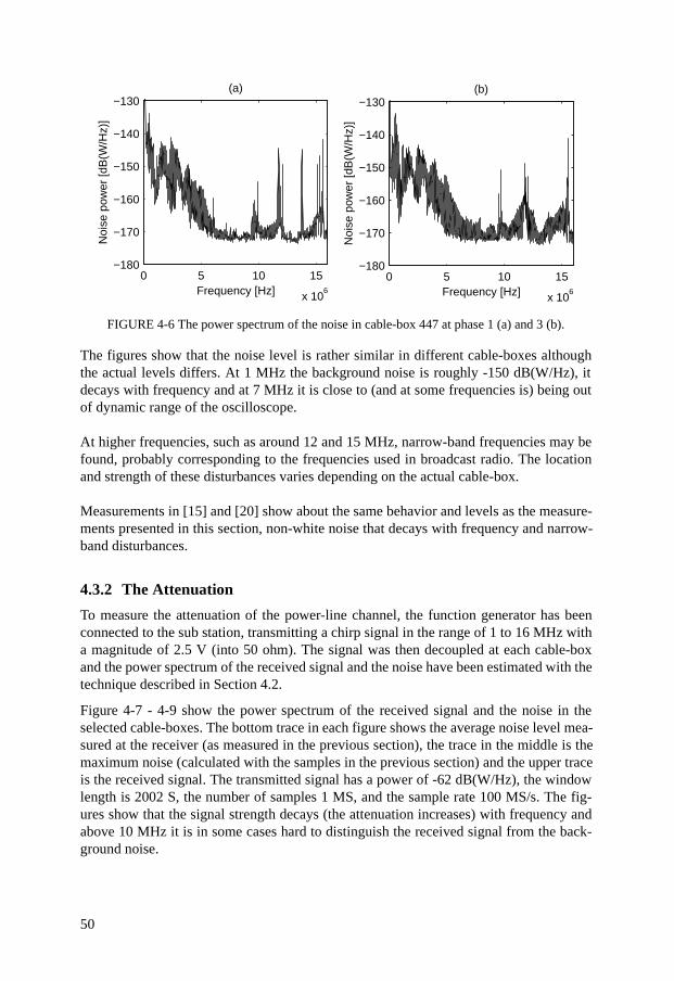
50

FIGURE 4-6 The power spectrum of the noise in cable-box 447 at phase 1 (a) and 3 (b).

The figures show that the noise level is rather similar in different cable-boxes althoughthe actual levels differs. At 1 MHz the background noise is roughly -150 dB(W/Hz), itdecays with frequency and at 7 MHz it is close to (and at some frequencies is) being outof dynamic range of the oscilloscope.

At higher frequencies, such as around 12 and 15 MHz, narrow-band frequencies may befound, probably corresponding to the frequencies used in broadcast radio. The locationand strength of these disturbances varies depending on the actual cable-box.

Measurements in [15] and [20] show about the same behavior and levels as the measure-ments presented in this section, non-white noise that decays with frequency and narrow-band disturbances.

4.3.2 The Attenuation

To measure the attenuation of the power-line channel, the function generator has beenconnected to the sub station, transmitting a chirp signal in the range of 1 to 16 MHz witha magnitude of 2.5 V (into 50 ohm). The signal was then decoupled at each cable-boxand the power spectrum of the received signal and the noise have been estimated with thetechnique described in Section 4.2.

Figure 4-7 - 4-9 show the power spectrum of the received signal and the noise in theselected cable-boxes. The bottom trace in each figure shows the average noise level mea-sured at the receiver (as measured in the previous section), the trace in the middle is themaximum noise (calculated with the samples in the previous section) and the upper traceis the received signal. The transmitted signal has a power of -62 dB(W/Hz), the windowlength is 2002 S, the number of samples 1 MS, and the sample rate 100 MS/s. The fig-ures show that the signal strength decays (the attenuation increases) with frequency andabove 10 MHz it is in some cases hard to distinguish the received signal from the back-ground noise.

0 5 10 15

x 106

−180

−170

−160

−150

−140

−130

Frequency [Hz]

Noi

se p

ower

[dB

(W/H

z)]

(a)

0 5 10 15

x 106

−180

−170

−160

−150

−140

−130

Frequency [Hz]

Noi

se p

ower

[dB

(W/H

z)]

(b)

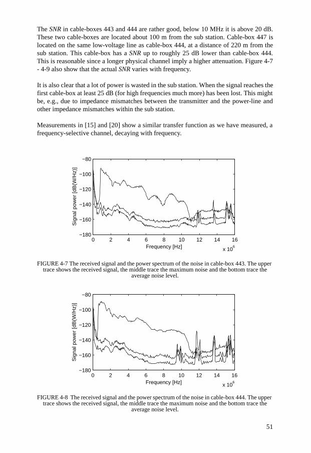
51

The SNR in cable-boxes 443 and 444 are rather good, below 10 MHz it is above 20 dB.These two cable-boxes are located about 100 m from the sub station. Cable-box 447 islocated on the same low-voltage line as cable-box 444, at a distance of 220 m from thesub station. This cable-box has a SNR up to roughly 25 dB lower than cable-box 444.This is reasonable since a longer physical channel imply a higher attenuation. Figure 4-7- 4-9 also show that the actual SNR varies with frequency.

It is also clear that a lot of power is wasted in the sub station. When the signal reaches thefirst cable-box at least 25 dB (for high frequencies much more) has been lost. This mightbe, e.g., due to impedance mismatches between the transmitter and the power-line andother impedance mismatches within the sub station.

Measurements in [15] and [20] show a similar transfer function as we have measured, afrequency-selective channel, decaying with frequency.

FIGURE 4-7 The received signal and the power spectrum of the noise in cable-box 443. The upper trace shows the received signal, the middle trace the maximum noise and the bottom trace the

average noise level.

FIGURE 4-8 The received signal and the power spectrum of the noise in cable-box 444. The upper trace shows the received signal, the middle trace the maximum noise and the bottom trace the

average noise level.

0 2 4 6 8 10 12 14 16

x 106

−180

−160

−140

−120

−100

−80

Frequency [Hz]

Sig

nal p

ower

[dB

(W/H

z)]

0 2 4 6 8 10 12 14 16

x 106

−180

−160

−140

−120

−100

−80

Frequency [Hz]

Sig

nal p

ower

[dB

(W/H

z)]

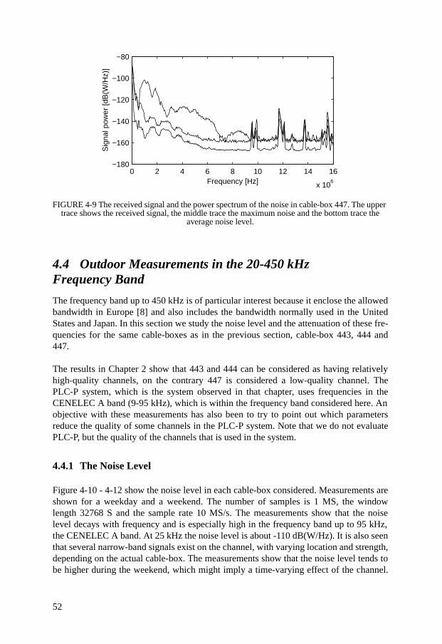
52

FIGURE 4-9 The received signal and the power spectrum of the noise in cable-box 447. The upper trace shows the received signal, the middle trace the maximum noise and the bottom trace the

average noise level.

4.4 Outdoor Measurements in the 20-450 kHz Frequency Band

The frequency band up to 450 kHz is of particular interest because it enclose the allowedbandwidth in Europe [8] and also includes the bandwidth normally used in the UnitedStates and Japan. In this section we study the noise level and the attenuation of these fre-quencies for the same cable-boxes as in the previous section, cable-box 443, 444 and447.

The results in Chapter 2 show that 443 and 444 can be considered as having relativelyhigh-quality channels, on the contrary 447 is considered a low-quality channel. ThePLC-P system, which is the system observed in that chapter, uses frequencies in theCENELEC A band (9-95 kHz), which is within the frequency band considered here. Anobjective with these measurements has also been to try to point out which parametersreduce the quality of some channels in the PLC-P system. Note that we do not evaluatePLC-P, but the quality of the channels that is used in the system.

4.4.1 The Noise Level

Figure 4-10 - 4-12 show the noise level in each cable-box considered. Measurements areshown for a weekday and a weekend. The number of samples is 1 MS, the windowlength 32768 S and the sample rate 10 MS/s. The measurements show that the noiselevel decays with frequency and is especially high in the frequency band up to 95 kHz,the CENELEC A band. At 25 kHz the noise level is about -110 dB(W/Hz). It is also seenthat several narrow-band signals exist on the channel, with varying location and strength,depending on the actual cable-box. The measurements show that the noise level tends tobe higher during the weekend, which might imply a time-varying effect of the channel.

0 2 4 6 8 10 12 14 16

x 106

−180

−160

−140

−120

−100

−80

Frequency [Hz]

Sig

nal p

ower

[dB

(W/H

z)]

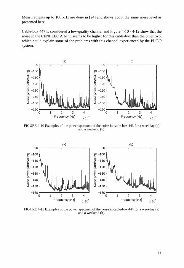
53

Measurements up to 100 kHz are done in [24] and shows about the same noise level aspresented here.

Cable-box 447 is considered a low-quality channel and Figure 4-10 - 4-12 show that thenoise in the CENELEC A band seems to be higher for this cable-box than the other two,which could explain some of the problems with this channel experienced by the PLC-Psystem.

FIGURE 4-10 Examples of the power spectrum of the noise in cable-box 443 for a weekday (a) and a weekend (b).

FIGURE 4-11 Examples of the power spectrum of the noise in cable-box 444 for a weekday (a) and a weekend (b).

0 1 2 3 4

x 105

−160

−150

−140

−130

−120

−110

−100

−90

Frequency [Hz]

Noi

se p

ower

[dB

(W/H

z)]

(a)

0 1 2 3 4

x 105

−160

−150

−140

−130

−120

−110

−100

−90

Frequency [Hz]

Noi

se p

ower

[dB

(W/H

z)]

(b)

0 1 2 3 4

x 105

−160

−150

−140

−130

−120

−110

−100

−90

Frequency [Hz]

Noi

se p

ower

[dB

(W/H

z)]

(a)

0 1 2 3 4

x 105

−160

−150

−140

−130

−120

−110

−100

−90

Frequency [Hz]

Noi

se p

ower

[dB

(W/H

z)]

(b)

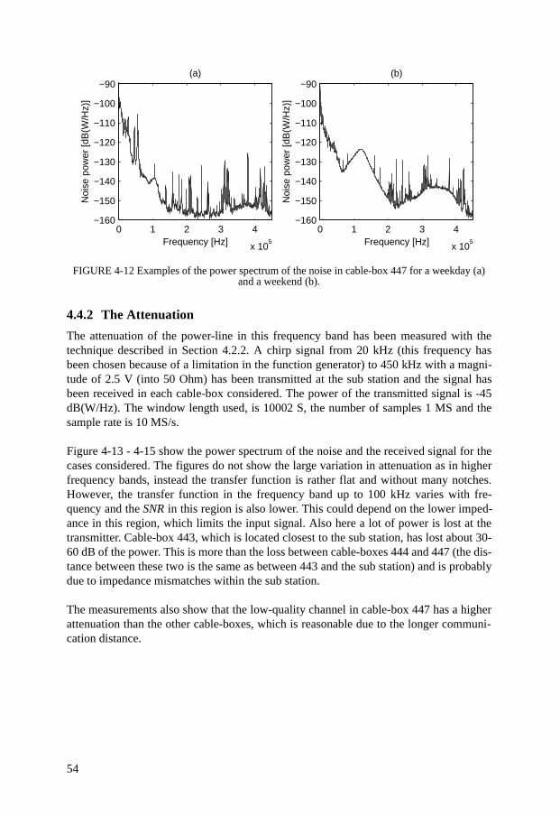
54

FIGURE 4-12 Examples of the power spectrum of the noise in cable-box 447 for a weekday (a) and a weekend (b).

4.4.2 The Attenuation

The attenuation of the power-line in this frequency band has been measured with thetechnique described in Section 4.2.2. A chirp signal from 20 kHz (this frequency hasbeen chosen because of a limitation in the function generator) to 450 kHz with a magni-tude of 2.5 V (into 50 Ohm) has been transmitted at the sub station and the signal hasbeen received in each cable-box considered. The power of the transmitted signal is -45dB(W/Hz). The window length used, is 10002 S, the number of samples 1 MS and thesample rate is 10 MS/s.

Figure 4-13 - 4-15 show the power spectrum of the noise and the received signal for thecases considered. The figures do not show the large variation in attenuation as in higherfrequency bands, instead the transfer function is rather flat and without many notches.However, the transfer function in the frequency band up to 100 kHz varies with fre-quency and the SNR in this region is also lower. This could depend on the lower imped-ance in this region, which limits the input signal. Also here a lot of power is lost at thetransmitter. Cable-box 443, which is located closest to the sub station, has lost about 30-60 dB of the power. This is more than the loss between cable-boxes 444 and 447 (the dis-tance between these two is the same as between 443 and the sub station) and is probablydue to impedance mismatches within the sub station.

The measurements also show that the low-quality channel in cable-box 447 has a higherattenuation than the other cable-boxes, which is reasonable due to the longer communi-cation distance.

0 1 2 3 4

x 105

−160

−150

−140

−130

−120

−110

−100

−90

Frequency [Hz]

Noi

se p

ower

[dB

(W/H

z)]

(a)

0 1 2 3 4

x 105

−160

−150

−140

−130

−120

−110

−100

−90

Frequency [Hz]

Noi

se p

ower

[dB

(W/H

z)]

(b)

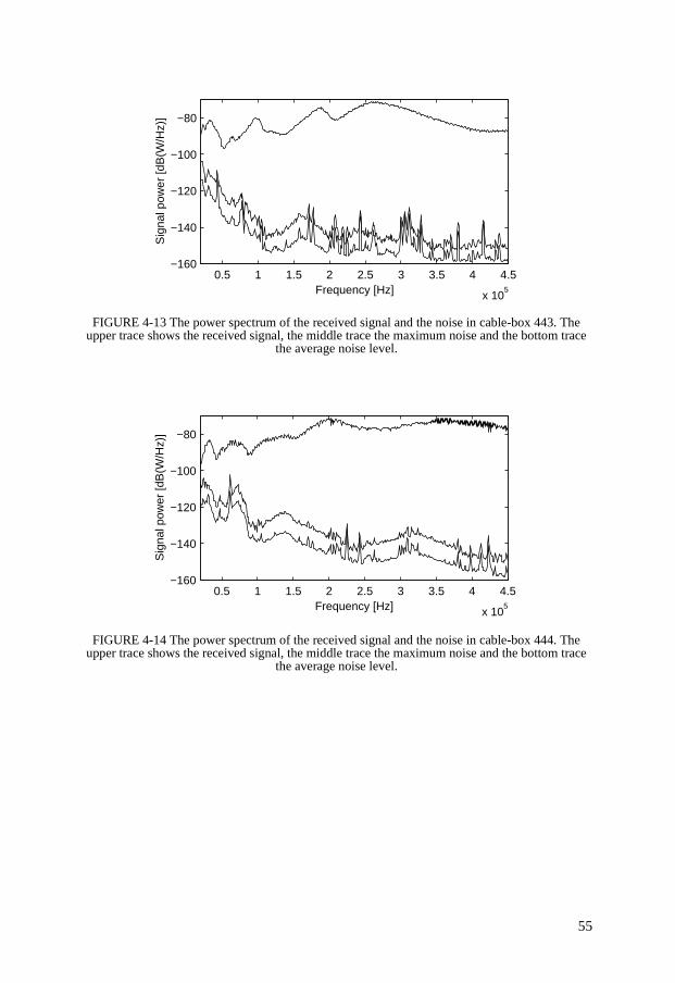
55

FIGURE 4-13 The power spectrum of the received signal and the noise in cable-box 443. The upper trace shows the received signal, the middle trace the maximum noise and the bottom trace

the average noise level.

FIGURE 4-14 The power spectrum of the received signal and the noise in cable-box 444. The upper trace shows the received signal, the middle trace the maximum noise and the bottom trace

the average noise level.

0.5 1 1.5 2 2.5 3 3.5 4 4.5

x 105

−160

−140

−120

−100

−80

Frequency [Hz]

Sig

nal p

ower

[dB

(W/H

z)]

0.5 1 1.5 2 2.5 3 3.5 4 4.5

x 105

−160

−140

−120

−100

−80

Frequency [Hz]

Sig

nal p

ower

[dB

(W/H

z)]

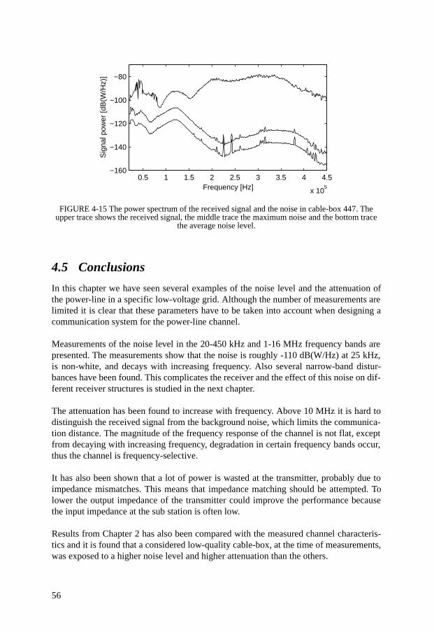
56

FIGURE 4-15 The power spectrum of the received signal and the noise in cable-box 447. The upper trace shows the received signal, the middle trace the maximum noise and the bottom trace

the average noise level.

4.5 Conclusions

In this chapter we have seen several examples of the noise level and the attenuation ofthe power-line in a specific low-voltage grid. Although the number of measurements arelimited it is clear that these parameters have to be taken into account when designing acommunication system for the power-line channel.

Measurements of the noise level in the 20-450 kHz and 1-16 MHz frequency bands arepresented. The measurements show that the noise is roughly -110 dB(W/Hz) at 25 kHz,is non-white, and decays with increasing frequency. Also several narrow-band distur-bances have been found. This complicates the receiver and the effect of this noise on dif-ferent receiver structures is studied in the next chapter.

The attenuation has been found to increase with frequency. Above 10 MHz it is hard todistinguish the received signal from the background noise, which limits the communica-tion distance. The magnitude of the frequency response of the channel is not flat, exceptfrom decaying with increasing frequency, degradation in certain frequency bands occur,thus the channel is frequency-selective.

It has also been shown that a lot of power is wasted at the transmitter, probably due toimpedance mismatches. This means that impedance matching should be attempted. Tolower the output impedance of the transmitter could improve the performance becausethe input impedance at the sub station is often low.

Results from Chapter 2 has also been compared with the measured channel characteris-tics and it is found that a considered low-quality cable-box, at the time of measurements,was exposed to a higher noise level and higher attenuation than the others.

0.5 1 1.5 2 2.5 3 3.5 4 4.5

x 105

−160

−140

−120

−100

−80

Frequency [Hz]

Sig

nal p

ower

[dB

(W/H

z)]

57

The measurements have also been compared to other measurements, which show similarbehavior and levels. It is important to do measurements at several locations and in differ-ent countries, to increase the understanding of the power-line as a communication chan-nel.

59

CHAPTER 5 Receiver Strategies for the Power-Line Communication Channel

5.1 Introduction

The previous chapter shows that the noise of the power-line channel can not be describedas AWGN (Additive White Gaussian Noise) [41], which is the case in many communica-tion models. In this chapter, we study the effect of this non-white noise on specificreceiver structures.

Though the characteristics of communication channels located at different positions inthe frequency domain can be quite different, many of the basic problems are the same.The coding and the modulation scheme has to be chosen in such a way that the receivedsignal energy, with high probability, is large enough such that the decision algorithm ofthe receiver efficiently can combat the disturbances.

The technical solution to this problem becomes harder as the ratio between informationbit rate and communication bandwidth is increased.

We apply Euclidean distance arguments to coded signal sequences in an attempt to quan-tify some effects of additive non-white gaussian noise on minimum Euclidean distancereceivers. A simple case with AWGN and narrow-band disturbances is considered. Tworeceiver structures are studied, and compared with respect to robustness against narrow-band disturbances. The reason we have chosen to study the Euclidean distance is its rela-tion to the error probability.

Convolutional coding, a fixed set of transmitter waveforms, and a frequency selectivecommunication channel are some underlying assumptions.

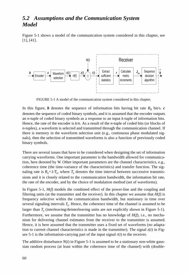
60

5.2 Assumptions and the Communication System Model

Figure 5-1 shows a model of the communication system considered in this chapter, see[1], [41].

FIGURE 5-1 A model of the communication system considered in this chapter.

In this figure, b denotes the sequence of information bits having bit rate Rb bit/s. cdenotes the sequence of coded binary symbols, and it is assumed that the encoder outputsan n-tuple of coded binary symbols as a response to an input k-tuple of information bits.Hence, the rate of the encoder is k/n. As a result of the n-tuple of coded bits (or blocks ofn-tuples), a waveform is selected and transmitted through the communication channel. Ifthere is memory in the waveform selection unit (e.g., continuous phase modulated sig-nals), then the selection of transmitted waveforms is also a function of previously codedbinary symbols.

There are several issues that have to be considered when designing the set of informationcarrying waveforms. One important parameter is the bandwidth allowed for communica-tion, here denoted by W. Other important parameters are the channel characteristics, e.g.,coherence time (the time-variance of the characteristics) and transfer function. The sig-naling rate is Rs=1/Ts, where Ts denotes the time interval between successive transmis-sions and it is closely related to the communication bandwidth, the information bit rate,the rate of the encoder, and by the choice of modulation method (set of waveforms).

In Figure 5-1, H(f) models the combined effect of the power-line and the coupling andfiltering units (at the transmitter and the receiver). In this chapter we assume that H(f) isfrequency selective within the communication bandwidth, but stationary in time overseveral signaling intervals Ts. Hence, the coherence time of the channel is assumed to belarger than Ts (interleaving/deinterleaving units are not explicitly shown in Figure 5-1).

Furthermore, we assume that the transmitter has no knowledge of H(f), i.e., no mecha-nism for delivering channel estimates from the receiver to the transmitter is assumed.Hence, it is here assumed that the transmitter uses a fixed set of waveforms (no adapta-tion to current channel characteristics is made in the transmitter). The signal z(t) in Fig-ure 5-1 is the information-carrying part of the input signal r(t) to the receiver.

The additive disturbance N(t) in Figure 5-1 is assumed to be a stationary non-white gaus-sian random process (at least within the coherence time of the channel) with (double-

Encoderb c Waveform

selections(t)

H(f)z(t) r(t)

N(t)

Extractsufficientstatistics

r Calculatemetric

increments

JincSequencedecisionalgorithm

b^

Receiver

61

sided) power spectrum where Pnarrow(f) represents the

narrow-band disturbances within the communication bandwidth W.

To arrive at simple expressions let us here assume that there are J equally strong narrow-band disturbances within the communication bandwidth W, and that the power in eachdisturbance, denoted by Pnb/J, is equally distributed over a frequency interval of length

∆, see Figure 5-2 (where J=5).

FIGURE 5-2 The power spectrum, RN(f), of the disturbance.

We define the parameter

(5-1)

as a measure of the strength of each of the narrow-band disturbances.

The sequence r in the receiver in Figure 5-1 contains the sufficient statistics extractedfrom the received signal r(t). Each element in the sequence r, r=(...,r[n-1], r[n],r[n+1],...), is in general a vector, and a new element is obtained every Ts seconds. Theoperations involved to obtain r typically consist of demodulation to baseband, bank ofmatched filters, and sampling with rate Rs.

For each element in r (or for a block of elements) a set of metric-increments, collected inthe vector Jinc[n], is calculated. The specific kind of metric used by the decision algo-rithm depends on several factors such as, coherent or non-coherent demodulation, soft orhard decisions, the amount of channel knowledge, level of complexity etc. In many caseshowever, it is desired to use a maximum likelihood based sequence detection algorithm,implemented with a state oriented approach like the Viterbi algorithm (i.e., the accumu-lated metric is recursively updated by metric-increments), see e.g., [41]. After a certaindecision delay, the receiver’s decision is available.

5.3 Two Receiver Structures

In this section we study the operation and detection performance of ideal coherent maxi-mum likelihood reception when the information-carrying signals are assumed to be dis-

RN f( ) N0 2⁄ Pnarrow f( )+=

f

∆ ∆ ∆ ∆ ∆W

N0

2

N02 +

Pnb/J2∆

xPnb J⁄

2∆---------------=

62

turbed by additive colored gaussian noise. Though the realization of such a receiver canbe impractical, it gives valuable insight in how a good suboptimal receiver could bedesigned. We try to quantify the gain obtained with such an ideal receiver, comparedwith a receiver which do not whiten the noise. Furthermore, the error performance of theideal receiver is (by definition) a lower bound on the performance of any practicalreceiver.

In an ideal situation when the receiver has complete knowledge of the power spectrumRN(f), and of the (overall) transfer function H(f), the sufficient statistics for detection canbe extracted as shown in Figure 5-3, see [1], [41], [51], [54].

FIGURE 5-3 A model of the first part of the ideal receiver

In Figure 5-3, the received signal is first filtered in a noise-whitening filter. Since the fil-ter is reversible within the communication bandwidth, no information is lost in this pro-cess. Hence, the noise in the signal x(t) is white within the communication bandwidth.The next filter in Figure 5-3 is a channel and noise matching filter (Th and Tw denotes thelength of the truncated channel impulse response and whitening filter respectively, and *denotes conjugate). This filter is followed by a bank of filters which are matched to thebasis functions required to describe the set of waveforms used in the transmitter. In Fig-ure 5-3 it is assumed that the basis functions are time-limited to Ts s. If they are not, addi-tional delay should be inserted in the filterbank (to make it causal). Note that the filtersused in Figure 5-3 are bandpass filters operating within the communication bandwidth. Apractical implementation often consists of demodulation to baseband, followed by low-pass filtering of the quadrature components. However, the method of implementation isnot critical for the present discussion.

The assumption that the receiver knows the set of basis functions, used in the transmitter,is a mild assumption. However, assuming knowledge of H(f) and RN(f) imply that mech-

anisms are implemented for providing the receiver with estimates of these functionswithin the coherence time of the channel (increased complexity). Furthermore, the noise-whitening filter introduces additional time-dispersion which can give severe intersymbolinterference if the signaling rate Rs is too high.

In the next two sections we investigate the ideal receiver (whitening approach, see Figure5-3), and also a suboptimal receiver which does not whiten the noise. The purpose is totry to evaluate, by simple arguments, the importance of the whitening filter and the chan-nel matching filter.

ejϕ(f)

RN(f)

x(t)r(t) H*(f)e-j(2πf(T + T )+ϕ(f))h w

RN(f)

G(f)

φ1(Ts-t)

φN(Ts-t)

r1[n]

rN[n]

r[n]

t=t0+nTs

... ...

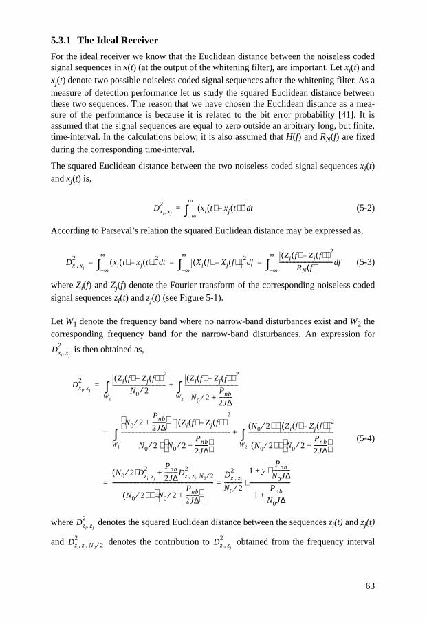
63

5.3.1 The Ideal Receiver

For the ideal receiver we know that the Euclidean distance between the noiseless codedsignal sequences in x(t) (at the output of the whitening filter), are important. Let xi(t) andxj(t) denote two possible noiseless coded signal sequences after the whitening filter. As ameasure of detection performance let us study the squared Euclidean distance betweenthese two sequences. The reason that we have chosen the Euclidean distance as a mea-sure of the performance is because it is related to the bit error probability [41]. It isassumed that the signal sequences are equal to zero outside an arbitrary long, but finite,time-interval. In the calculations below, it is also assumed that H(f) and RN(f) are fixed

during the corresponding time-interval.

The squared Euclidean distance between the two noiseless coded signal sequences xi(t)and xj(t) is,

(5-2)

According to Parseval’s relation the squared Euclidean distance may be expressed as,

(5-3)

where Zi(f) and Zj(f) denote the Fourier transform of the corresponding noiseless codedsignal sequences zi(t) and zj(t) (see Figure 5-1).

Let W1 denote the frequency band where no narrow-band disturbances exist and W2 thecorresponding frequency band for the narrow-band disturbances. An expression for

is then obtained as,

(5-4)

where denotes the squared Euclidean distance between the sequences zi(t) and zj(t)

and denotes the contribution to obtained from the frequency interval

Dxi xj,2

xi t( ) xj t( )–( )2td

∞–

∞

∫=

Dxi xj,2

xi t( ) xj t( )–( )2td

∞–

∞

∫ Xi f( ) Xj f( )–( ) 2fd

∞–

∞

∫Zi f( ) Zj f( )–( ) 2

RN f( )--------------------------------------- fd

∞–

∞

∫= = =

Dxi xj,2

Dxi xj,2 Zi f( ) Zj f( )–( ) 2

N0 2⁄---------------------------------------

W1

∫Zi f( ) Zj f( )–( ) 2

N0 2⁄Pnb

2J∆----------+

---------------------------------------

W2

∫+=

N0 2⁄Pnb

2J∆----------+

Zi f( ) Zj f( )–( )⋅2

N0 2⁄ N0 2⁄Pnb

2J∆----------+

⋅--------------------------------------------------------------------------------

W1

∫N0 2⁄( ) Zi f( ) Zj f( )–( )⋅ 2

N0 2⁄( ) N0 2⁄Pnb

2J∆----------+

⋅--------------------------------------------------------------

W2

∫+=

N0 2⁄( )Dzi zj,2 Pnb

2J∆----------Dzi zj N0 2⁄, ,

2+

N0 2⁄( ) N0 2⁄Pnb

2J∆----------+

⋅--------------------------------------------------------------------------

Dzi zj,2

N0 2⁄-------------

1 yPnb

N0J∆-------------⋅+

1Pnb

N0J∆-------------+

------------------------------⋅==

Dzi zj,2

Dzi zj N0 2⁄, ,2

Dzi zj,2

64

within the communication bandwidth, where . The parameter y is defined

as,

(5-5)

and is a measure of the relative distance contribution (in z(t)), due to the AWGN fre-quency intervals only. y is a parameter of i and j and is determined by the two signalsequences that the receiver compares.

The largest value of y is y=1 which imply that in this ideal case. Hence, no

loss in Euclidean distance is then obtained since the narrow-band disturbances and thedifference signal zi(t)-zj(t) are located in disjoint frequency bands. Similarly, the smallestvalue of y is y=0, which represents the worst case for a given RN(f). Furthermore, from

(5-4) it is seen that if the total power Pnb in the narrow-band disturbances is increased,

then will approach the value . For small values of Pnb, the value of is

not so sensitive to the precise value of y.

As a measure of the performance loss due to the narrow-band disturbances we calculatethe squared Euclidean distance reduction, in dB. When no narrow-band disturbances

exist the squared Euclidean distance is and if we divide (5-4) with this distance we

get the reduction,

(5-6)

It is not possible to guarantee that always is large enough (the error probability low

enough) since H(f) and RN(f) are frequency dependent, random, and not known inadvance. If, however, the fixed set of transmitter waveforms is designed to cover a largepart of the communication bandwidth (frequency diversity), then signal energy will bedelivered in all passbands of the current channel. This strategy will also promote a highvalue of y, especially if the communication bandwidth is large compared with the band-width occupied by the narrow-band disturbances (=J∆).

5.3.2 The Suboptimal Receiver

In this subsection it is assumed that the filter g(t) in Figure 5-3 is chosen such that

RN f( ) N0 2⁄=

yDzi zj N0 2⁄, ,

2

Dzi zj,2

-------------------------=

Dxi xj,2 Dzi zj,

2

N0 2⁄-------------=

Dxi xj,2

yDzi zj,

2

N0 2⁄------------- Dxi xj,

2

Dzi zj,2

N0 2⁄-------------

10

1 yPnb

N0J∆-------------+

1Pnb

N0J∆-------------+

--------------------------

log

Dxi xj,2

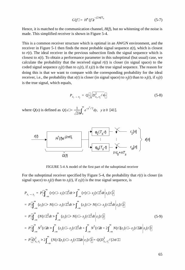
65

(5-7)

Hence, it is matched to the communication channel, H(f), but no whitening of the noise ismade. This simplified receiver is shown in Figure 5-4.

This is a common receiver structure which is optimal in an AWGN environment, and thereceiver in Figure 5-1 then finds the most probable signal sequence z(t), which is closestto r(t). The ideal receiver in the previous subsection finds the signal sequence which isclosest to x(t). To obtain a performance parameter in this suboptimal (but usual) case, wecalculate the probability that the received signal r(t) is closer (in signal space) to thecoded signal sequence zj(t) than to zi(t), if zi(t) is the true signal sequence. The reason fordoing this is that we want to compare with the corresponding probability for the idealreceiver, i.e., the probability that x(t) is closer (in signal space) to xj(t) than to xi(t), if xi(t)is the true signal, which equals,

(5-8)

where Q(x) is defined as [41].

FIGURE 5-4 A model of the first part of the suboptimal receiver

For the suboptimal receiver specified by Figure 5-4, the probability that r(t) is closer (insignal space) to zj(t) than to zi(t), if zi(t) is the true signal sequence, is

(5-9)

G f( ) H∗ f( )ej2πfTh–

=

Pxi xj→ Q Dxi xj,2

4⁄ =

Q x( ) 1

2π---------- e

y2

2⁄–yd

x

∞

∫= y 0≥,

r(t) H*(f)e-j2πfTh

G(f)

φ1(Ts-t)

φN(Ts-t)

r1[n]

rN[n]

r[n]

t=t0+nTs

... ...

Pzi zj→ P r t( ) zi t( )–( )2td

∞–

∞

∫ r t( ) zj t( )–( )2td

∞–

∞

∫> zi t( ) =

P zi t( ) N t( ) zi t( )–+( )2td

∞–

∞

∫ zi t( ) N t( ) zj t( )–+( )2td

∞–

∞

∫> zi t( ) =

P N t( )( )2td

∞–

∞

∫ zi t( ) N t( ) zj t( )–+( )2td

∞–

∞

∫> zi t( ) =

P N2

t( ) td∞–

∞

∫ zi t( ) zj t( )–( )2td

∞–

∞

∫ N2

t( ) td∞–

∞

∫ 2 N t( ) zi t( ) zj t( )–( ) td∞–

∞

∫+ +> zi t( ) =

P Dzi zj,2

2 N t( ) zi t( ) zj t( )–( )( ) td∞–

∞

∫> zi t( ) Q Dzi zj,

22σ( )⁄( )==

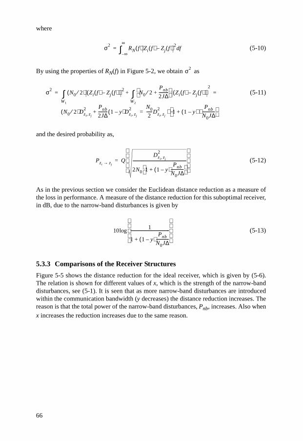
66

where

(5-10)

By using the properties of RN(f) in Figure 5-2, we obtain as

(5-11)

and the desired probability as,

(5-12)

As in the previous section we consider the Euclidean distance reduction as a measure ofthe loss in performance. A measure of the distance reduction for this suboptimal receiver,in dB, due to the narrow-band disturbances is given by

(5-13)

5.3.3 Comparisons of the Receiver Structures

Figure 5-5 shows the distance reduction for the ideal receiver, which is given by (5-6).The relation is shown for different values of x, which is the strength of the narrow-banddisturbances, see (5-1). It is seen that as more narrow-band disturbances are introducedwithin the communication bandwidth (y decreases) the distance reduction increases. Thereason is that the total power of the narrow-band disturbances, Pnb, increases. Also whenx increases the reduction increases due to the same reason.

σ2RN f( ) Zi f( ) Zj f( )–

2fd

∞–

∞

∫=

σ2

σ2N0 2⁄( ) Zi f( ) Zj f( )–( ) 2

W1

∫ N0 2⁄Pnb

2J∆----------+

Zi f( ) Zj f( )–( )2

W2

∫+

N0 2⁄( )Dzi zj,2 Pnb

2J∆---------- 1 y–( )Dzi zj,

2+

N0

2------Dzi zj,

21 1 y–( )

Pnb

N0J∆-------------⋅+

⋅

= =

=

Pzi zj→ QDzi zj,

2

2N0 1 1 y–( )Pnb

N0J∆-------------+

-------------------------------------------------------

=

101

1 1 y–( )Pnb

N0J∆-------------+

----------------------------------------

log

67

FIGURE 5-5 Distance reduction for the ideal receiver as a function of the parameters x and y defined in (5-1) and (5-5). Examples are shown when x = 1, 2, 5, 10, 20, 100. The dashed line

shows an upper limit of the distance reduction.

Figure 5-6 shows the distance reduction (5-13) for the suboptimal receiver. The figureshows that the narrow-band disturbances hurt this receiver significantly harder than theideal receiver. This is reasonable because no attempt has been made to compensate forthe colored noise. We see that when the parameter y decreases (more and/or wider nar-row-band disturbances are introduced within the communication bandwidth), thereceiver gets a high distance reduction, which also reduces the error probability of thecommunication system.

FIGURE 5-6 Distance reduction for the suboptimal receiver as a function of the parameters x and y defined in (5-1) and (5-5). Examples are shown when x = 1, 2, 5, 10, 20, 100.

By comparing the arguments in (5-8) and in (5-12) we get an indication of the differencein performance between the two studied receivers. The ratio between these arguments(expressed in dB) is

0 0.5 1−25

−20

−15

−10

−5

0

y

Dis

tanc

e re

duct

ion

[dB

]

x=1

x=100

0 0.5 1−25

−20

−15

−10

−5

0

y

Dis

tanc

e re

duct

ion

[dB

]

x=1

x=100

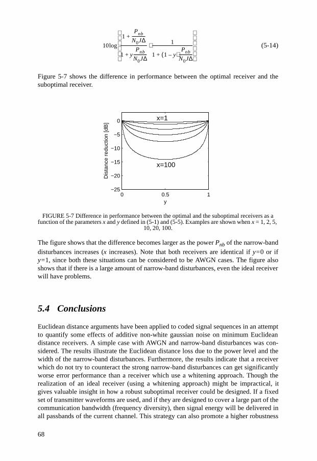
68

(5-14)

Figure 5-7 shows the difference in performance between the optimal receiver and thesuboptimal receiver.

FIGURE 5-7 Difference in performance between the optimal and the suboptimal receivers as a function of the parameters x and y defined in (5-1) and (5-5). Examples are shown when x = 1, 2, 5,

10, 20, 100.

The figure shows that the difference becomes larger as the power Pnb of the narrow-banddisturbances increases (x increases). Note that both receivers are identical if y=0 or ify=1, since both these situations can be considered to be AWGN cases. The figure alsoshows that if there is a large amount of narrow-band disturbances, even the ideal receiverwill have problems.

5.4 Conclusions

Euclidean distance arguments have been applied to coded signal sequences in an attemptto quantify some effects of additive non-white gaussian noise on minimum Euclideandistance receivers. A simple case with AWGN and narrow-band disturbances was con-sidered. The results illustrate the Euclidean distance loss due to the power level and thewidth of the narrow-band disturbances. Furthermore, the results indicate that a receiverwhich do not try to counteract the strong narrow-band disturbances can get significantlyworse error performance than a receiver which use a whitening approach. Though therealization of an ideal receiver (using a whitening approach) might be impractical, itgives valuable insight in how a robust suboptimal receiver could be designed. If a fixedset of transmitter waveforms are used, and if they are designed to cover a large part of thecommunication bandwidth (frequency diversity), then signal energy will be delivered inall passbands of the current channel. This strategy can also promote a higher robustness

10

1Pnb

N0J∆-------------+

1 yPnb

N0J∆-------------+

-------------------------- 1

1 1 y–( )Pnb

N0J∆-------------+

----------------------------------------⋅

log

0 0.5 1−25

−20

−15

−10

−5

0

y

Dis

tanc

e re

duct

ion

[dB

]

x=1

x=100

69

against narrow-band disturbances, for the two receiver structures studied, especially ifthe communication bandwidth is large compared with the bandwidth occupied by thesedisturbances. There are several possible modulation methods that could be considered aspossible candidates for power-line communication, e.g., Orthogonal Frequency DivisionMultiplex (OFDM) [18], Continuous Phase Modulation (CPM), and Code Division Mul-tiple Access (CDMA) [41]. However, many additional technical aspects should also beconsidered (besides regulatory issues). An example is the technical solution of the equal-izer (e.g., channel matching filter) which depends on the choice of modulation method.

70

71

CHAPTER 6 A Modulation Method for the Power-Line Communication Channel

As we have seen in previous chapters the power-line channel is a harsh environment. Thecharacteristics of the channel tend to vary in time, location and with different loads. Thestudy in Chapter 2 describes this behavior.

One possible solution to overcome the problems with such a channel, is to use a robustmodulation method. Furthermore, if the modulation method is able to handle unknownattenuation and unknown phase shifts, then the receiver can be simplified. The problemis to combine these requirements with the high bit rate needed in today’s computer com-munications and the bandwidth limitation on the power-line channel.

The intention with this chapter is to present a modulation that may be a candidate to beused in a communication system for the power-line channel. Here, the focus is on theerror probability properties, for the considered set of uncoded information carrying sig-nals, when these are detected non-coherently. In a practical system (coded) these signalsmight be combined with a chosen encoder and interleaver structure. This is also dis-cussed in the end of this chapter, using known properties of the power-line channel.

The disposition of the chapter is as follows:

Section 6.1 gives a general description of the modulation method. Section 6.2 showscomputer-simulated results of the performance of the method and Section 6.3 theoreti-cally validates the simulations. In Section 6.4 we combine the method with coding,diversity and the use of sub-bands. Finally Section 6.5 concludes the results.

6.1 The Modulation Method

Figure 6-1 shows a model of the communication system considered in this chapter, [1],[41], [54]. The transmitter transmits a signal, s(t), on the channel, which is modeled as a

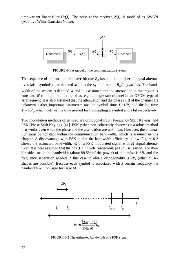
72

time-variant linear filter H(f,t). The noise at the receiver, N(t), is modeled as AWGN(Additive White Gaussian Noise).

FIGURE 6-1 A model of the communication system.

The sequence of information bits have bit rate Rb b/s and the number of signal alterna-

tives (also symbols), are denoted M, thus the symbol rate is b/s. The band-

width of the system is denoted W and it is assumed that the attenuation in this region isconstant. W can here be interpreted as, e.g., a single sub-channel in an OFDM-type ofarrangement. It is also assumed that the attenuation and the phase shift of the channel areunknown. Other important parameters are the symbol time Ts=1/Rs and the bit time

Tb=1/Rb, which defines the time needed for transmitting a symbol and a bit respectively.

Two modulation methods often used are orthogonal FSK (Frequency Shift Keying) andPSK (Phase Shift Keying) [41]. FSK (when non-coherently detected) is a robust methodthat works even when the phase and the attenuation are unknown. However, the attenua-tion must be constant within the communication bandwidth, which is assumed in thischapter. A disadvantage with FSK is that the bandwidth efficiency is low. Figure 6-2shows the estimated bandwidth, W, of a FSK modulated signal with M signal alterna-tives. It is here assumed that the hcs (Half Cycle Sinusoidal) [41] pulse is used. The dou-ble sided mainlobe bandwidth (about 99.5% of the power) of this pulse is 3Rs and thefrequency separation needed in this case to obtain orthogonality is 2Rs (other pulse-

shapes are possible). Because each symbol is associated with a certain frequency thebandwidth will be large for large M.

FIGURE 6-2 The estimated bandwidth of a FSK signal.

Transmitter ReceiverH(f,t)

N(t)

s(t) z(t) r(t)

Rb log2M⁄

sR2

1f 2f 1−Mf Mf

( )bR

M

MW

2log

12 +=

f

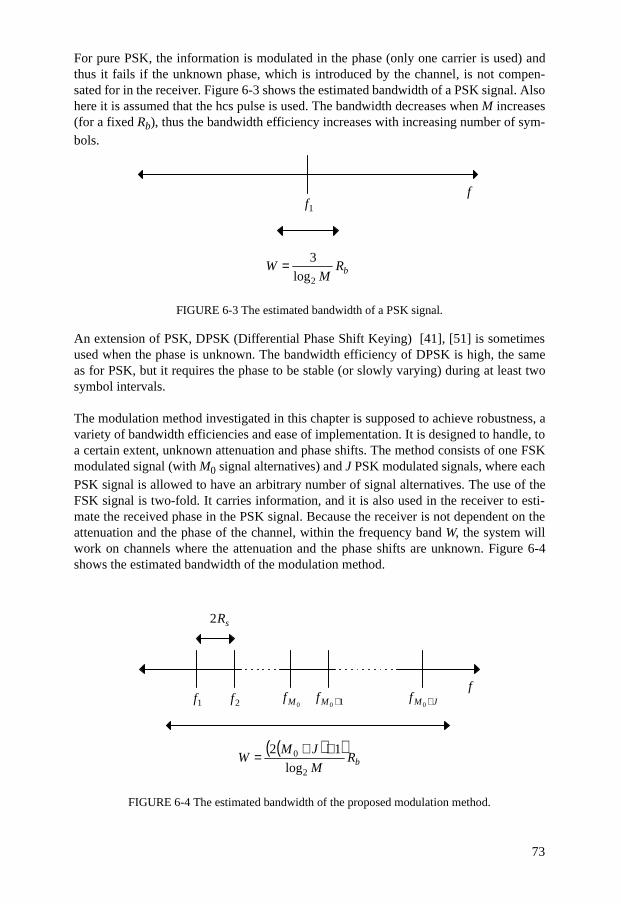
73

For pure PSK, the information is modulated in the phase (only one carrier is used) andthus it fails if the unknown phase, which is introduced by the channel, is not compen-sated for in the receiver. Figure 6-3 shows the estimated bandwidth of a PSK signal. Alsohere it is assumed that the hcs pulse is used. The bandwidth decreases when M increases(for a fixed Rb), thus the bandwidth efficiency increases with increasing number of sym-bols.

FIGURE 6-3 The estimated bandwidth of a PSK signal.

An extension of PSK, DPSK (Differential Phase Shift Keying) [41], [51] is sometimesused when the phase is unknown. The bandwidth efficiency of DPSK is high, the sameas for PSK, but it requires the phase to be stable (or slowly varying) during at least twosymbol intervals.

The modulation method investigated in this chapter is supposed to achieve robustness, avariety of bandwidth efficiencies and ease of implementation. It is designed to handle, toa certain extent, unknown attenuation and phase shifts. The method consists of one FSKmodulated signal (with M0 signal alternatives) and J PSK modulated signals, where eachPSK signal is allowed to have an arbitrary number of signal alternatives. The use of theFSK signal is two-fold. It carries information, and it is also used in the receiver to esti-mate the received phase in the PSK signal. Because the receiver is not dependent on theattenuation and the phase of the channel, within the frequency band W, the system willwork on channels where the attenuation and the phase shifts are unknown. Figure 6-4shows the estimated bandwidth of the modulation method.

FIGURE 6-4 The estimated bandwidth of the proposed modulation method.

1f

bRM

W2log

3=

f

sR2

1f 2f 0Mf

( )( )bR

M

JMW

2

0

log

12 ++=

f10 +Mf JMf +0

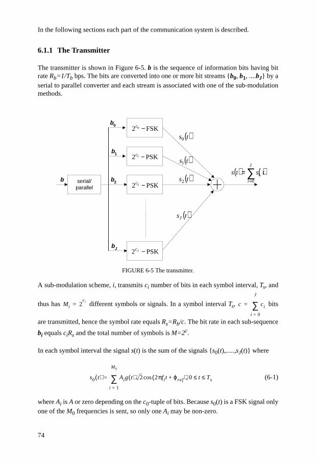
74

In the following sections each part of the communication system is described.

6.1.1 The Transmitter

The transmitter is shown in Figure 6-5. b is the sequence of information bits having bitrate Rb=1/Tb bps. The bits are converted into one or more bit streams {b0, b1, ....bJ} by a

serial to parallel converter and each stream is associated with one of the sub-modulationmethods.

FIGURE 6-5 The transmitter.

A sub-modulation scheme, i, transmits ci number of bits in each symbol interval, Ts, and

thus has different symbols or signals. In a symbol interval Ts, bits

are transmitted, hence the symbol rate equals Rs=Rb/c. The bit rate in each sub-sequence

bi equals ciRs and the total number of symbols is M=2c.

In each symbol interval the signal s(t) is the sum of the signals {s0(t),.....,sJ(t)} where

(6-1)

where Ai is A or zero depending on the c0-tuple of bits. Because s0(t) is a FSK signal onlyone of the M0 frequencies is sent, so only one Ai may be non-zero.

serial/parallel

FSK2 0 −c

PSK2 1 −c

PSK2 2 −c

PSK2 −Jc

( )ts0

( )ts1

( )ts2

( )tsJ

( ) ( )∑=

=J

ii tsts

0b

b0

b1

b2

bJ

Mi 2ci= c ci

i 0=

J

∑=

s0 t( ) Aig t( ) 2 2πfit ϕref+( )cos

i 1=

M0

∑= 0 t Ts≤ ≤,

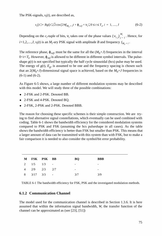
75

The PSK-signals, si(t), are described as,

(6-2)

Depending on the ci-tuple of bits, νi takes one of the phase values . Hence, for

i=1,2,....,J, si(t) is an Mi-ary PSK signal with amplitude B and frequency .

The reference phase, ϕref, must be the same for all the (M0+J) frequencies in the interval

0<t<Ts. However, ϕref is allowed to be different in different symbol intervals. The pulse-shape g(t) is not specified but typically the half cycle sinusoidal (hcs) pulse may be used.The energy of g(t), Eg, is assumed to be one and the frequency spacing is chosen suchthat an 2(M0+J)-dimensional signal space is achieved, based on the M0+J frequencies in(6-1) and (6-2).

As Figure 6-5 shows, a large number of different modulation systems may be describedwith this model. We will study three of the possible combinations:

• 2-FSK and 2-PSK. Denoted BB.

• 2-FSK and 4-PSK. Denoted BQ.

• 2-FSK, 2-PSK and 2-PSK. Denoted BBB.

The reason for choosing these specific schemes is their simple construction. We are try-ing to find alternative signal constellations, which eventually can be used combined withcoding. Table 6-1 shows the bandwidth efficiency for the considered modulation systemscompared to PSK and FSK (assuming the hcs pulseshape in all cases). As the tableshows the bandwidth efficiency is better than FSK but smaller than PSK. This means thata larger amount of data can be transmitted with this system than with FSK, but to make afair comparison it is needed to also consider the symbol/bit error probability.

TABLE 6-1 The bandwidth efficiency for FSK, PSK and the investigated modulation methods.

6.1.2 Communication Channel

The model used for the communication channel is described in Section 1.3.6. It is hereassumed that within the information signal bandwidth, W, the transfer function of thechannel can be approximated as (see [23], [51])

M FSK PSK BB BQ BBB

2 1/5 1/3 - - -

4 2/9 2/3 2/7 - -

8 3/17 3/3 - 3/7 3/9

si t( ) Bg t( ) 2 2πfM0 i+ t ϕref νi+ +( )cos= 0 t Ts i,≤ ≤, 1 .... J, ,=

νi j,{ }j 1=

Mi

fM0 i+

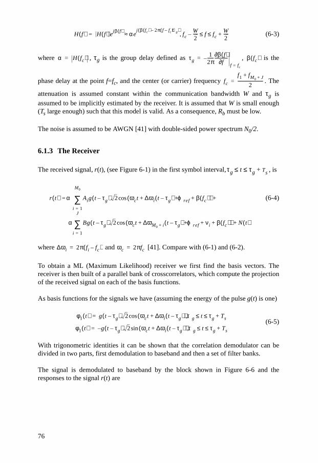
76

(6-3)

where , τg is the group delay defined as , is the

phase delay at the point f=fc, and the center (or carrier) frequency . The

attenuation is assumed constant within the communication bandwidth W and τg isassumed to be implicitly estimated by the receiver. It is assumed that W is small enough(Ts large enough) such that this model is valid. As a consequence, Rb must be low.

The noise is assumed to be AWGN [41] with double-sided power spectrum N0/2.

6.1.3 The Receiver

The received signal, r(t), (see Figure 6-1) in the first symbol interval, , is

(6-4)

where and [41]. Compare with (6-1) and (6-2).

To obtain a ML (Maximum Likelihood) receiver we first find the basis vectors. Thereceiver is then built of a parallel bank of crosscorrelators, which compute the projectionof the received signal on each of the basis functions.

As basis functions for the signals we have (assuming the energy of the pulse g(t) is one)

(6-5)

With trigonometric identities it can be shown that the correlation demodulator can bedivided in two parts, first demodulation to baseband and then a set of filter banks.

The signal is demodulated to baseband by the block shown in Figure 6-6 and theresponses to the signal r(t) are

H f( ) H f( ) ejβ f( ) αe

j β fc( ) 2π f fc–( )τg–( )fc

W2-----– f fc

W2-----+≤ ≤,≈=

α H fc( )= τg1

2π------ β f( )∂

f∂-------------–

f fc=

= β fc( )

fc

f1 fM0 J++

2-------------------------=

τg t τg Ts+≤ ≤

r t( ) α Aig t τg–( ) 2 ωct ∆ωi t τg–( ) ϕref β fc( )+ + +( )cos

i 1=

M0

∑

α Bg t τg–( ) 2 ωct ∆ωM0 i+ t τg–( ) ϕref νi β fc( )+ + + +( )cos

i 1=

J

∑ N t( )

+

+

=

∆ωi 2π fi fc–( )= ωc 2πfc=

φ1 t( ) g t τg–( ) 2 ωct ∆ωi t τg–( )+( ) τg t τg Ts+≤ ≤,cos=

φ1 t( ) g t τg–( )– 2 ωct ∆ωi t τg–( )+( ) τg t τg Ts+≤ ≤,sin=

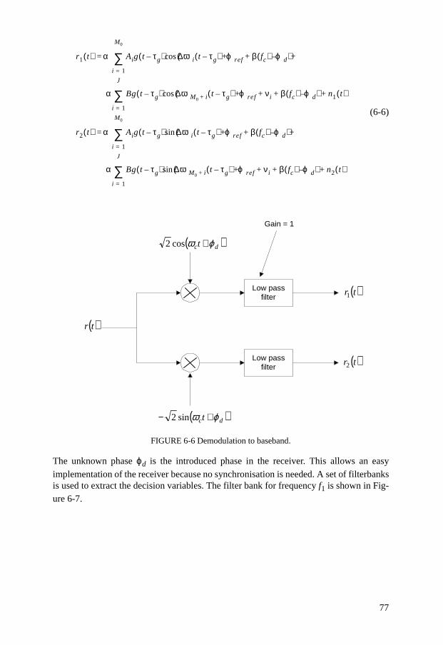
77

(6-6)

FIGURE 6-6 Demodulation to baseband.

The unknown phase ϕd is the introduced phase in the receiver. This allows an easy

implementation of the receiver because no synchronisation is needed. A set of filterbanksis used to extract the decision variables. The filter bank for frequency f1 is shown in Fig-ure 6-7.

r1 t( ) α Aig t τg–( ) ∆ωi t τg–( ) ϕref β fc( ) ϕd–+ +( )+cos

i 1=

M0

∑=

α Bg t τg–( ) ∆ωM0 i+ t τg–( ) ϕref νi β fc( ) ϕd–+ + +( ) n1 t( )+cos

i 1=

J

∑

r2 t( ) α Aig t τg–( ) ∆ωi t τg–( ) ϕref β fc( ) ϕd–+ +( )+sin

i 1=

M0

∑=

α Bg t τg–( ) ∆ωM0 i+ t τg–( ) ϕref νi β fc( ) ϕd–+ + +( )sin

i 1=

J

∑ n2 t( )+

Low passfilter

( )dct ϕω +cos2

Low passfilter

( )dct ϕω +− sin2

( )tr1

( )tr2

( )tr

Gain = 1

78

FIGURE 6-7 The filter bank for frequency f1.

The responses to the filters in Figure 6-7 are:

(6-7)

(6-8)

where

(6-9)

Assuming that Eg=1 then W1,1 and W1,2 are independent Gaussian random variableswith variance N0/2 and mean zero.

If these calculations are repeated for ∆ω2... then the set of complex decision

variables obtained is:

(6-10)

where

(6-11)

( ) ( )( )tTtTg ss −∆− 1cos ω

( ) ( )( )tTtTg ss −∆− 1sin ω

( ) ( )( )tTtTg ss −∆− 1cos ω

( ) ( )( )tTtTg ss −∆− 1sin ω( )tr1

( )tr2

1,1x

2,1x

sg Tt +=τ

x1 1, αA1Eg

θ( )cos2

---------------- n1 1, αA1Eg

θ( )cos2

---------------- n1 2,+ + + αA1Eg

θ( )cos W1 1,+= =

x1 2, αA1Eg

θ( )sin2

--------------- n2 1, αA1Eg

θ( )sin2

--------------- n2 2,+ + + αA1Eg

θ( )sin W1 2,+= =

θ ϕref β fc( ) ϕd–+=

W1 1, n1 1, n1 2,+=

W1 2, n2 1, n2 2,+=

∆ωM0 J+

Xi αAiejθ

Wi+ i, 1 2,...,M0,= =

Yi αBejνie

jθWi M0++ i, 1 2 .... J,,,= =

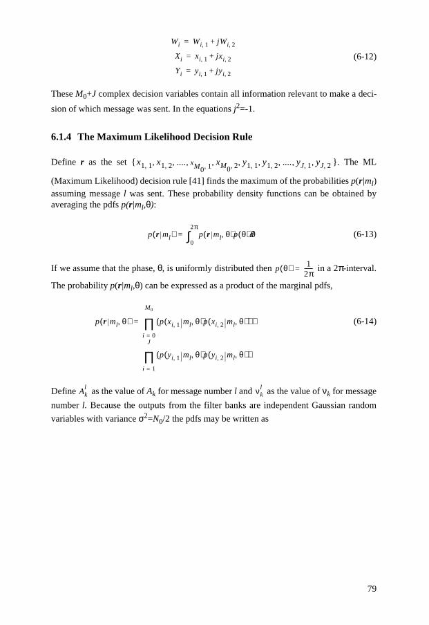
79

(6-12)

These M0+J complex decision variables contain all information relevant to make a deci-

sion of which message was sent. In the equations j2=-1.

6.1.4 The Maximum Likelihood Decision Rule

Define r as the set { }. The ML

(Maximum Likelihood) decision rule [41] finds the maximum of the probabilities p(r|ml)assuming message l was sent. These probability density functions can be obtained byaveraging the pdfs p(r|ml,θ):

(6-13)

If we assume that the phase, θ, is uniformly distributed then in a 2π-interval.

The probability p(r|ml,θ) can be expressed as a product of the marginal pdfs,

(6-14)

Define as the value of Ak for message number l and as the value of νk for message

number l. Because the outputs from the filter banks are independent Gaussian random

variables with variance σ2=N0/2 the pdfs may be written as

Wi Wi 1, jWi 2,+=

Xi xi 1, jxi 2,+=

Yi yi 1, jyi 2,+=

x1 1, x1 2, .... xM0 1, xM0 2, y1 1, y1 2, .... yJ 1, yJ 2,, , , , , , , , ,

p r ml( ) p r ml θ,( )p θ( ) θd0

2π

∫=

p θ( ) 12π------=

p r ml θ,( ) p xi 1, ml θ,( )p xi 2, ml θ,( )( )

p yi 1, ml θ,( )p yi 2, ml θ,( )( )i 1=

J

∏

⋅i 0=

M0

∏=

Akl νk

l

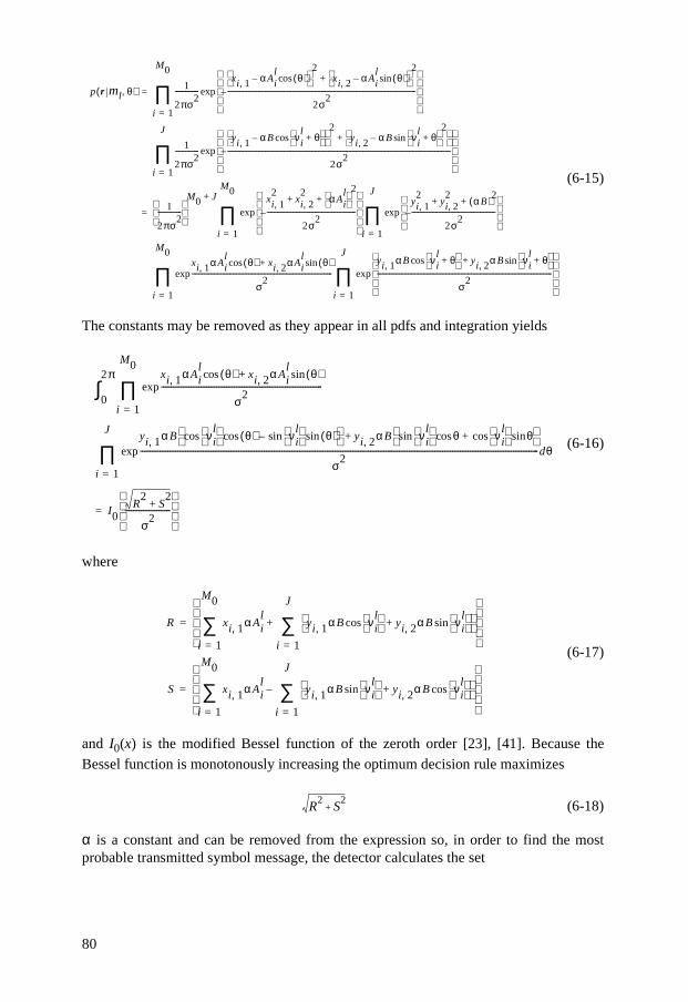
80

(6-15)

The constants may be removed as they appear in all pdfs and integration yields

(6-16)

where

(6-17)

and I0(x) is the modified Bessel function of the zeroth order [23], [41]. Because the

Bessel function is monotonously increasing the optimum decision rule maximizes

(6-18)

α is a constant and can be removed from the expression so, in order to find the mostprobable transmitted symbol message, the detector calculates the set

p r ml θ,( ) 1

2πσ2--------------

xi 1, αAil θ( )cos–

2

xi 2, αAil θ( )sin–

2

+

2σ2--------------------------------------------------------------------------------------------------------------–

exp

i 1=

M0

∏=

1

2πσ2--------------

yi 1, αB νil θ+

cos–

2yi 2, αB νi

l θ+ sin–

2

+

2σ2----------------------------------------------------------------------------------------------------------------------------------–

exp

i 1=

J

∏

1

2πσ2

--------------

M0 J+ xi 1,2

xi 2,2 αAi

l

2+ +

2σ2----------------------------------------------------–

yi 1,2

yi 2,2 αB( )2+ +

2σ2-------------------------------------------------–

exp

i 1=

J

∏exp

i 1=

M0

∏=

xi 1, αAil θ( )cos xi 2, αAi

l θ( )sin+

σ2

----------------------------------------------------------------------------------yi 1, αB νi

l θ+ cos yi 2, αB νi

l θ+ sin+

σ2

------------------------------------------------------------------------------------------------------

exp

i 1=

J

∏exp

i 1=

M0

∏

xi 1, αAil θ( )cos xi 2, αAi

l θ( )sin+

σ2----------------------------------------------------------------------------------exp

i 1=

M0

∏0

2π∫

yi 1, αB νil

θ( )coscos νi

l sin θ( )sin–

yi 2, αB νil

θcossin νi

l cos θsin+

+

σ2-----------------------------------------------------------------------------------------------------------------------------------------------------------------------------------------------------------dθexp

i 1=

J

∏

I0R

2S2

+

σ2-----------------------

=

R xi 1, αAil

i 1=

M0

∑ yi 1, αB νil

yi 2, αB νi

l sin+cos

i 1=

J

∑+

=

S xi 1, αAil

i 1=

M0

∑ yi 1, αB νil

yi 2, αB νi

l cos+sin

i 1=

J

∑–

=

R2

S2

+

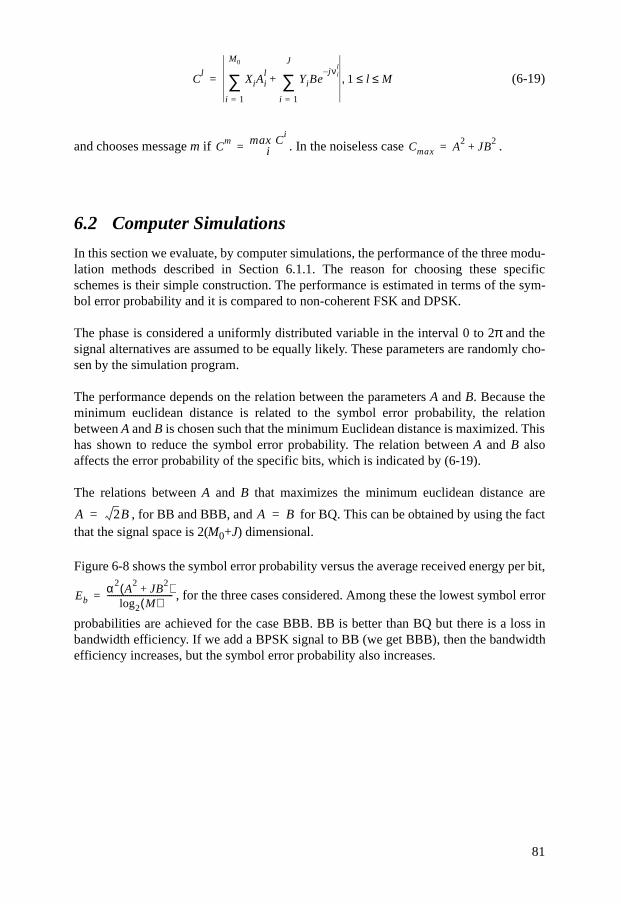
81

(6-19)

and chooses message m if . In the noiseless case .

6.2 Computer Simulations

In this section we evaluate, by computer simulations, the performance of the three modu-lation methods described in Section 6.1.1. The reason for choosing these specificschemes is their simple construction. The performance is estimated in terms of the sym-bol error probability and it is compared to non-coherent FSK and DPSK.

The phase is considered a uniformly distributed variable in the interval 0 to 2π and thesignal alternatives are assumed to be equally likely. These parameters are randomly cho-sen by the simulation program.

The performance depends on the relation between the parameters A and B. Because theminimum euclidean distance is related to the symbol error probability, the relationbetween A and B is chosen such that the minimum Euclidean distance is maximized. Thishas shown to reduce the symbol error probability. The relation between A and B alsoaffects the error probability of the specific bits, which is indicated by (6-19).

The relations between A and B that maximizes the minimum euclidean distance are

, for BB and BBB, and for BQ. This can be obtained by using the factthat the signal space is 2(M0+J) dimensional.

Figure 6-8 shows the symbol error probability versus the average received energy per bit,

, for the three cases considered. Among these the lowest symbol error

probabilities are achieved for the case BBB. BB is better than BQ but there is a loss inbandwidth efficiency. If we add a BPSK signal to BB (we get BBB), then the bandwidthefficiency increases, but the symbol error probability also increases.

Cl

XiAil

i 1=

M0

∑ YiBejνi

l–

i 1=

J

∑+ 1 l M≤ ≤,=

Cm max C

i

i= Cmax A2

JB2

+=

A 2B= A B=

Ebα2

A2

JB2

+( )log2 M( )

---------------------------------=

82

FIGURE 6-8 The symbol error probability for the three systems considered.

Figure 6-9 shows the symbol error probability compared to DPSK and Figure 6-10shows the symbol error probability compared to non-coherent FSK (NCFSK). The sys-tems are compared with the same number of signal alternatives. The symbol error proba-bilities for DPSK and FSK are not simulated but calculated, see [41], [51].

Figure 6-9 shows that the symbol error probability for BB is about the same as for 4-DPSK, but at the cost of lower bandwidth efficiency. To increase the bandwidth effi-ciency BQ can be used. Then there is a loss in energy efficiency but the symbol errorprobability is better than 8-DPSK. The same is achieved with BBB. The symbol errorprobability for non-coherent FSK is, in the cases considered, lower than the proposedmethods, but the bandwidth efficiency is not as good. We can conclude that the symbolerror probability is somewhat between non-coherent FSK and DPSK, and this also holdsfor the bandwidth efficiency.

2 3 4 5 6 7 8 9 1010

−4

10−3

10−2

10−1

100

Eb/N

0

Ps

BBB

BQ

BB

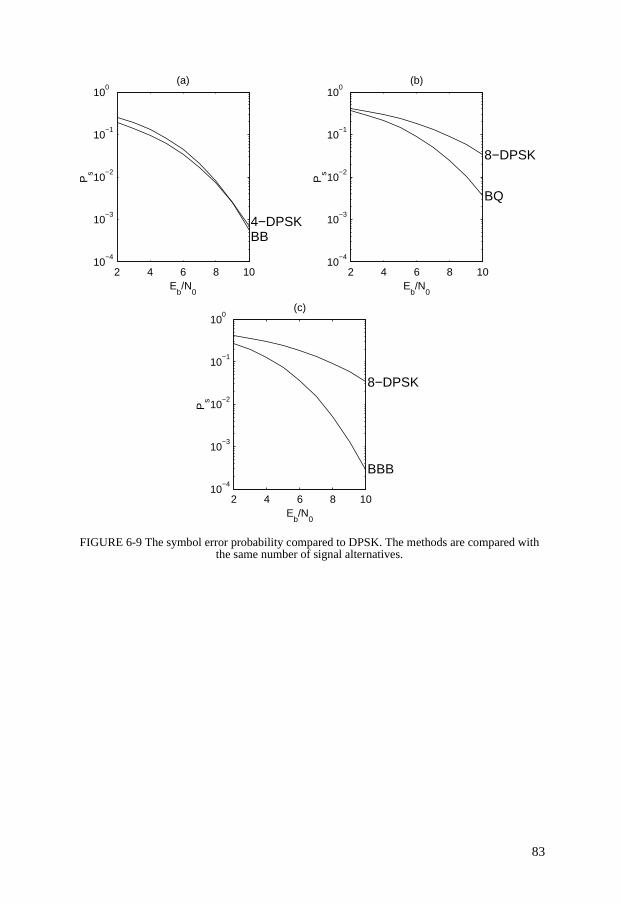
83

FIGURE 6-9 The symbol error probability compared to DPSK. The methods are compared with the same number of signal alternatives.

2 4 6 8 1010

−4

10−3

10−2

10−1

100

Eb/N

0

Ps

BB4−DPSK

(a)

2 4 6 8 1010

−4

10−3

10−2

10−1

100

Eb/N

0

Ps

BQ

8−DPSK

(b)

2 4 6 8 1010

−4

10−3

10−2

10−1

100

Eb/N

0

Ps

BBB

8−DPSK

(c)

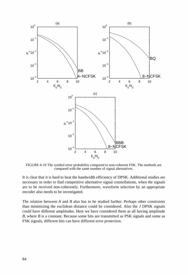
84

FIGURE 6-10 The symbol error probability compared to non-coherent FSK. The methods are compared with the same number of signal alternatives.

It is clear that it is hard to beat the bandwidth efficiency of DPSK. Additional studies arenecessary in order to find competitive alternative signal constellations, when the signalsare to be received non-coherently. Furthermore, waveform selection by an appropriateencoder also needs to be investigated.

The relation between A and B also has to be studied further. Perhaps other constraintsthan minimizing the euclidean distance could be considered. Also the J DPSK signalscould have different amplitudes. Here we have considered them as all having amplitudeB, where B is a constant. Because some bits are transmitted as PSK signals and some asFSK signals, different bits can have different error protection.

2 4 6 8 1010

−4

10−3

10−2

10−1

100

Eb/N

0

Ps

BB4−NCFSK

(a)

2 4 6 8 1010

−4

10−3

10−2

10−1

100

Eb/N

0

Ps

BQ

8−NCFSK

(b)

2 4 6 8 1010

−4

10−3

10−2

10−1

100

Eb/N

0

Ps

BBB8−NCFSK

(c)

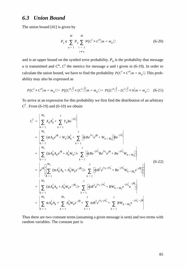
85

6.3 Union Bound

The union bound [41] is given by

(6-20)

and is an upper bound on the symbol error probability. Pu is the probability that message

u is transmitted and Cu, Ci the metrics for message u and i given in (6-19). In order to

calculate the union bound, we have to find the probability . This prob-

ability may also be expressed as

(6-21)

To arrive at an expression for this probability we first find the distribution of an arbitrary

Cl . From (6-19) and (6-10) we obtain

(6-22)

Thus there are two constant terms (assuming a given message is sent) and two terms withrandom variables. The constant part is

Ps Pu P Ci

Cu

m mu=>( )i 1=

i u≠

M

∑u 1=

M

∑≤

P Ci

Cu

m mu=>( )

P Ci

Cu

m mu=>( ) P Cu( )

2C

i( )2

< m mu=( ) P Cu( )

2C

i( )2

– 0< m mu=( )= =

Cl

XkAkl

k 1=

M0

∑ YkBejνk

l–

k 1=

J

∑+=

αAkejθ

Wk+( )Akl

k 1=

M0

∑ αBejvke

jθWk M0++

Bejνk

l–

k 1=

J

∑+=

αAklAke

jθAk

lWk+( )

k 1=

M0

∑ αBejνk

l–Be

jvkejθ

Bejνk

l–Wk M0++

k 1=

J

∑+=

ejθ αAk

lAk Ak

lWke

j– θ+( )k 1=

M0

∑ αB2e

jvk jνkl–

Bejνk

l–Wk M0+ e

j– θ+

k 1=

J

∑+

=

αAklAk Ak

lWke

j– θ+( )

k 1=

M0

∑ αB2e

jvk jνkl

–BWk M0+ e

jνkl

–e

j– θ+

k 1=

J

∑+=

αAklAk

k 1=

M0

∑ AklWke

j– θ

k 1=

M0

∑ αB2e

jvk jνkl–

k 1=

J

∑ BWk M0+ ejνk

l– jθ–

k 1=

J

∑+ + +=

86

(6-23)

and the random part

(6-24)

(6-25)

Because Wi,j are independent Gaussian random variables with variance N0/2 and zero-mean the variance of the real part in (6-25) is (given θ)

αAklAk

k 1=

M0

∑ αB2e

jvk jνkl

–

k 1=

J

∑+

αAklAk

k 1=

M0

∑ αB2

vk νkl

–( )cos

k 1=

J

∑+

j αB2

vk νkl

–( )sin

k 1=

J

∑

+=

AklWke

j– θ

k 1=

M0

∑ BWk M0+ ejνk

l– jθ–

k 1=

J

∑+

AklWk θ( )cos

k 1=

M0

∑ j AklWk θ( )sin

k 1=

M0

∑–=

+ BWk M0+ νkl

– θ–( )cos

k 1=

J

∑ j BWk M0+ νkl

– θ–( )sin

k 1=

J

∑+

Akl

Wk 1, jWk 2,+( ) θ( )cos

k 1=

M0

∑ j Akl

Wk 1, jWk 2,+( ) θ( )sin

k 1=

M0

∑–=

+ B Wk M0+ 1, jWk M0+ 2,+( ) νkl

– θ–( )cos

k 1=

J

∑

+j B Wk M0+ 1, jWk M0+ 2,+( ) νkl

– θ–( )sin

k 1=

J

∑

AklWk 1, θ( )cos

k 1=

M0

∑ AklWk 2, θ( )sin

k 1=

M0

∑+=

+ BWk M0+ 1, νkl

– θ–( )cos

k 1=

J

∑ BWk M0+ 2, νkl

– θ–( )sin

k 1=

J

∑–

j AklWk 1, θ( )sin

k 1=

M0

∑– j AklWk 2, θ( )cos

k 1=

M0

∑+

+j BWk M0+ 2, νkl

– θ–( )cos

k 1=

J

∑ j BWk M0+ 1, νkl

– θ–( )sin

i 1=

J

∑+

87

(6-26)

and in the same way the variance of the complex part in (6-25) is

(6-27)

Define the variables X and Y such that

(6-28)

Assume message u is transmitted, then X and Y are complex-valued Gaussian randomvariables (see [41]) with mean

(6-29)

The covariance of the random variables X and Y is

Akl( )

2N0

2------ θ( )cos( )2

k 1=

M0

∑ Akl( )

2N0

2------ θ( )sin( )2

k 1=

M0

∑+

+ B2N0

2------ νk

l– θ–( )cos( )

2

k 1=

J

∑ B2N0

2------ νk

l– θ–( )sin( )

2

i k=

J

∑+

A2N0

2------ JB

2N0

2------+=

Akl( )

2N0

2------ θ( )cos( )2

k 1=

M0

∑ Akl( )

2N0

2------ θ( )sin( )2

k 1=

M0

∑+

+ B2N0

2------ νk

l– θ–( )cos( )

2

k 1=

J

∑ B2N0

2------ νk

l– θ–( )sin( )

2

k 1=

J

∑+

A2N0

2------ JB

2N0

2------+=

X2

Cu( )

2=

Y2

Ci( )

2=

X αAkuAk

u

k 1=

M0

∑ αB2

vku νk

u–( )cos

k 1=

J

∑+

j αB2

vku νk

u–( )sin

k 1=

J

∑

+=

Y αAkiAk

u

k 1=

M0

∑ αB2

vku νk

i–( )cos

k 1=

J

∑+

j αB2

vku νk

i–( )sin

k 1=

J

∑

+=

88

(6-30)

Using the fact that the product of two independent zero-mean random processes has zeromean, and the trigonometric identities

(6-31)

we arrive at

σXY2 1

2---E X X–( ) Y Y–( )

* =

12---E= [ ( Ak

uWk 1, θ( )cos

k 1=

M0

∑ Aku

Wk 2, θ( )sin

k 1=

M0

∑+

+ BWk M0+ 1, νku

– θ– cos

k 1=

J

∑ BWk M0+ 2, νku

– θ– sin

k 1=

J

∑–

+j Aku

Wk 2, θ( )cos

k 1=

M0

∑ j Aku

Wk 1, θ( ) sin

k 1=

M0

∑–

+ j BWk M0+ 2, νku

– θ– cos

k 1=

J

∑ j BWk M0+ 1, νku

– θ– ) sin

k 1=

J

∑+

( Aki

Wk 1, θ( )cos

k 1=

M0

∑ Aki

Wk 2, θ( )sin

k 1=

M0

∑+

+ BWk M0+ 1, νki

– θ– cos

k 1=

J

∑ BWk M0+ 2, νki

– θ– sin

k 1=

J

∑–

j Aki

Wk 2, θ( )cos

k 1=

M0

∑– j Aki

Wk 1, θ( )sin

k 1=

M0

∑+

j BWk M0+ 2, νki

– θ– cos

k 1=

J

∑ j BWk M0+ 1, νki

– θ– )]sin

k 1=

J

∑––

α β–( )sin α βcossin α βsincos–=

α β–( )cos αcos βcos αsin βsin+=

89

(6-32)

If we simplify this we get

(6-33)

(6-34)

where (the mean of ) is equal to N0/2. The variance of a complex-valued ran-

dom variable Z is given by

(6-35)

Similar calculations as above yields the variance of X and Y

σXY2 1

2---E( Ak

uAk

iWk 1,

2 θ( )cos( )2

k 1=

M0

∑= AkuAk

iWk 1,

2 θ( )sin( )2

k 1=

M0

∑+

+ AkuAk

iWk 2,

2 θ( )sin( )2

k 1=

M0

∑ AkuAk

iWk 2,

2 θ( )cos( )2

k 1=

M0

∑+

+ B2Wk M0+ 2,

2 νku

– θ– νki

– θ–( )–( )cos

k 1=

J

∑

+j B2Wk M0+ 2,

2 νku

– θ– νki

– θ–( )–( )sin

k 1=

J

∑

+ B2Wk M0+ 1,

2 νku

– θ– νki

– θ–( )–( )cos

k 1=

J

∑

+j B2Wk M0+ 1,

2 νku

– θ– νki

– θ–( )–( ))sin

k 1=

J

∑

σXY2 1

2---E( Ak

uAk

iWk 1,

2

k 1=

M0

∑= AkuAk

iWk 2,

2

k 1=

M0

∑+

+ B2Wk M0+ 2,

2 νku

– νki

+( )cos

k 1=

J

∑ j B2Wk M0+ 2,

2 νku

– νki

+( )sin

k 1=

J

∑+

+ B2Wk M0+ 1,

2 νku

– νki

+( )cos

k 1=

J

∑ j B2Wk M0+ 1,

2 νku

– νki

+( ))sin

k 1=

J

∑+

σXY2 µ

W2( )=

12---E( Ak

uAk

i

k 1=

M0

∑ AkuAk

i

k 1=

M0

∑ B2 νk

u– νk

i+( )cos

k 1=

J

∑+ +

+j B2 νk

u– νk

i+( )sin

k 1=

J

∑ B2 νk

u– νk

i+( )cos

k 1=

J

∑ j B2 νk

u– νk

i+( ))sin

k 1=

J

∑+ +

µW

2 Wi j,2

σZ2 1

2---E Z Z–( ) Z Z–( )

*( )=

90

(6-36)

This is also seen by setting i = u in (6-34).

Using X and Y the probability may be written as

(6-37)

This probability is a special case of a quadratic form given in [41], where it is shown that

(6-38)

where

(6-39)

I0(x) is the zeroth-order modified Bessel function of the first kind and Q1(x) is the gener-alized Marcum’s Q-function.

If we consider (6-20) we see that it is now possible to calculate the union bound. Figure6-11 - 6-13 show the union bound for each system assuming equally likely signal alterna-tives. Each figure also shows the simulated symbol error probability. The figures clearlyshow that, for high signal to noise ratios, the union bound approaches the simulatedresults.

σX2 σY

2 µW

2 A2

JB2

+( )= =

P Cu( )

2C

i( )2

– 0< m mu=( )

P X2

Y2

– 0< m mu=( )

P X2

Y2

– 0< m mu=( ) Q1 a b,( )v2 v1⁄

1 v2 v1⁄+-----------------------I0 ab( ) 1

2---– a

2b

2+( )

exp–=

Q1 a b,( ) x12---– x

2a

2+( )

I0 ax( )exp xdb

∞

∫=

a2v1

2v2 α1v2 α2–( )

v1 v2+( )2-------------------------------------------=

b2v1v2

2 α1v1 α2+( )

v1 v2+( )2--------------------------------------------=

α1 2 X2σYY

2Y

2σXX

2X

*YσXY

2– XY

*σXY

2( )*

–+( )=

α2 X2

Y2

–( )=

v1 w2 1

4 σXX2 σYY

2 σXY2 2

–( )-------------------------------------------------+ w–=

v2 w2 1

4 σXX2 σYY

2 σXY2 2

–( )-------------------------------------------------+ w+=

wσXX

2 σYY2

–

4 σXX2 σYY

2 σXY2 2

–( )------------------------------------------------- 0= =

91

FIGURE 6-11 The union bound of the symbol error probability (the dashed line) and the simulated error probability (the solid line) for BB.

FIGURE 6-12 The union bound of the symbol error probability (the dashed line) and the simulated error probability (the solid line) for BQ.

2 4 6 8 10 1210

−5

10−4

10−3

10−2

10−1

100

Eb/N

0

Ps

2 4 6 8 10 1210

−5

10−4

10−3

10−2

10−1

100

Eb/N

0

Ps

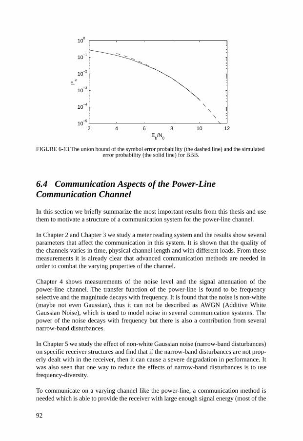
92

FIGURE 6-13 The union bound of the symbol error probability (the dashed line) and the simulated error probability (the solid line) for BBB.

6.4 Communication Aspects of the Power-Line Communication Channel

In this section we briefly summarize the most important results from this thesis and usethem to motivate a structure of a communication system for the power-line channel.

In Chapter 2 and Chapter 3 we study a meter reading system and the results show severalparameters that affect the communication in this system. It is shown that the quality ofthe channels varies in time, physical channel length and with different loads. From thesemeasurements it is already clear that advanced communication methods are needed inorder to combat the varying properties of the channel.

Chapter 4 shows measurements of the noise level and the signal attenuation of thepower-line channel. The transfer function of the power-line is found to be frequencyselective and the magnitude decays with frequency. It is found that the noise is non-white(maybe not even Gaussian), thus it can not be described as AWGN (Additive WhiteGaussian Noise), which is used to model noise in several communication systems. Thepower of the noise decays with frequency but there is also a contribution from severalnarrow-band disturbances.

In Chapter 5 we study the effect of non-white Gaussian noise (narrow-band disturbances)on specific receiver structures and find that if the narrow-band disturbances are not prop-erly dealt with in the receiver, then it can cause a severe degradation in performance. Itwas also seen that one way to reduce the effects of narrow-band disturbances is to usefrequency-diversity.

To communicate on a varying channel like the power-line, a communication method isneeded which is able to provide the receiver with large enough signal energy (most of the

2 4 6 8 10 1210

−5

10−4

10−3

10−2

10−1

100

Eb/N

0

Ps

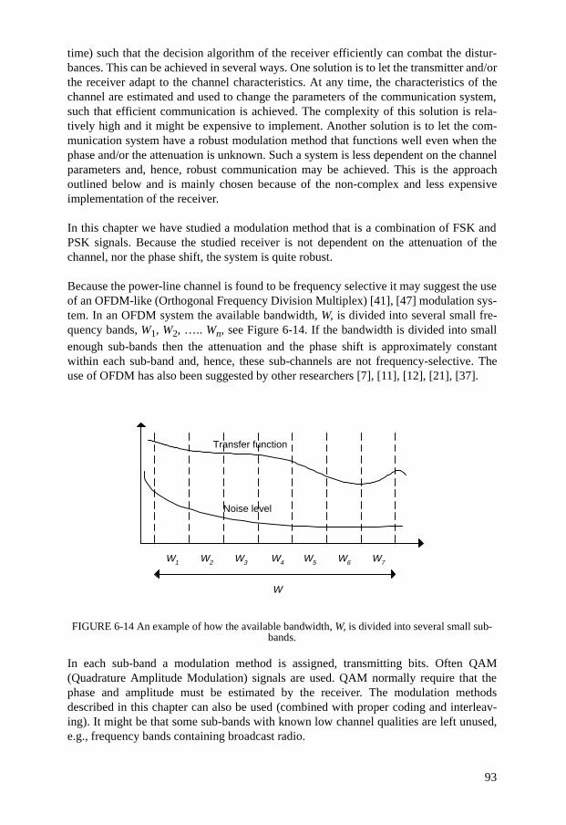
93

time) such that the decision algorithm of the receiver efficiently can combat the distur-bances. This can be achieved in several ways. One solution is to let the transmitter and/orthe receiver adapt to the channel characteristics. At any time, the characteristics of thechannel are estimated and used to change the parameters of the communication system,such that efficient communication is achieved. The complexity of this solution is rela-tively high and it might be expensive to implement. Another solution is to let the com-munication system have a robust modulation method that functions well even when thephase and/or the attenuation is unknown. Such a system is less dependent on the channelparameters and, hence, robust communication may be achieved. This is the approachoutlined below and is mainly chosen because of the non-complex and less expensiveimplementation of the receiver.

In this chapter we have studied a modulation method that is a combination of FSK andPSK signals. Because the studied receiver is not dependent on the attenuation of thechannel, nor the phase shift, the system is quite robust.

Because the power-line channel is found to be frequency selective it may suggest the useof an OFDM-like (Orthogonal Frequency Division Multiplex) [41], [47] modulation sys-tem. In an OFDM system the available bandwidth, W, is divided into several small fre-quency bands, W1, W2, ….. Wn, see Figure 6-14. If the bandwidth is divided into smallenough sub-bands then the attenuation and the phase shift is approximately constantwithin each sub-band and, hence, these sub-channels are not frequency-selective. Theuse of OFDM has also been suggested by other researchers [7], [11], [12], [21], [37].

FIGURE 6-14 An example of how the available bandwidth, W, is divided into several small sub-bands.

In each sub-band a modulation method is assigned, transmitting bits. Often QAM(Quadrature Amplitude Modulation) signals are used. QAM normally require that thephase and amplitude must be estimated by the receiver. The modulation methodsdescribed in this chapter can also be used (combined with proper coding and interleav-ing). It might be that some sub-bands with known low channel qualities are left unused,e.g., frequency bands containing broadcast radio.

Noise level

Transfer function

W

W1 W2 W3 W4 W5 W7W6

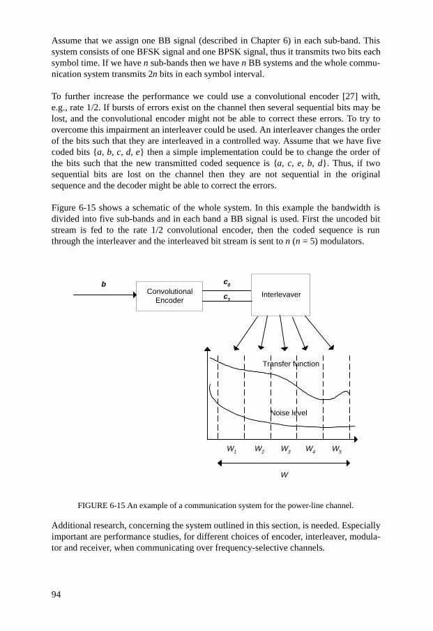
94

Assume that we assign one BB signal (described in Chapter 6) in each sub-band. Thissystem consists of one BFSK signal and one BPSK signal, thus it transmits two bits eachsymbol time. If we have n sub-bands then we have n BB systems and the whole commu-nication system transmits 2n bits in each symbol interval.

To further increase the performance we could use a convolutional encoder [27] with,e.g., rate 1/2. If bursts of errors exist on the channel then several sequential bits may belost, and the convolutional encoder might not be able to correct these errors. To try toovercome this impairment an interleaver could be used. An interleaver changes the orderof the bits such that they are interleaved in a controlled way. Assume that we have fivecoded bits {a, b, c, d, e} then a simple implementation could be to change the order ofthe bits such that the new transmitted coded sequence is {a, c, e, b, d}. Thus, if twosequential bits are lost on the channel then they are not sequential in the originalsequence and the decoder might be able to correct the errors.

Figure 6-15 shows a schematic of the whole system. In this example the bandwidth isdivided into five sub-bands and in each band a BB signal is used. First the uncoded bitstream is fed to the rate 1/2 convolutional encoder, then the coded sequence is runthrough the interleaver and the interleaved bit stream is sent to n (n = 5) modulators.

FIGURE 6-15 An example of a communication system for the power-line channel.

Additional research, concerning the system outlined in this section, is needed. Especiallyimportant are performance studies, for different choices of encoder, interleaver, modula-tor and receiver, when communicating over frequency-selective channels.

ConvolutionalEncoder

Interlevaver

Noise level

Transfer function

W

W1 W2 W3 W4 W5

b c0

c1

95

6.5 Conclusions

In this chapter we have studied a set of modulation methods, which are able to handleunknown phase and attenuation. The reason of doing this is that we want to come upwith a communication system with a simple implementation of the receiver. The systemconsists of one FSK signal and one or more PSK signals, where the FSK signal is used toestimate the received phase for the PSK signals.

It is shown, theoretically and by simulations, that the symbol error probability is higherthan for non-coherent FSK and lower than for DPSK, and the same holds for the band-width efficiency. This system may be a candidate to be used in power-line communica-tions, but more studies are needed in order to know if the modulation is competitive,especially combined with coding.

This modulation is used combined with coding, frequency diversity and the use of sub-channels (similar to Orthogonal Frequency Division Multiplex) to propose a communi-cation system for the power-line channel. The result is a flexible structure which can beupgraded and adapted to future needs.

97

CHAPTER 7 Conclusions

This thesis is about power-line communication, communication over the existing power-lines. The main advantage of this kind of communication system is the existing infra-structure, which simplifies the implementation. We start this thesis, after a general intro-duction to power-line communication, by doing some measurements of basic properties,to understand the behavior of the power-line as a communication channel. Then we usethese results combined with coding, modulation methods, different receiver structures,diversity and coding to present a communication strategy for the power-line channel.

In Chapter 2 we study an existing application, using the low-voltage grid as a communi-cation channel. By observing this system it has been possible to extract information ofwhich properties that affect the communication on the power-line channel. Propertiesthat we have seen affect the communication are: different time-windows, the location inthe grid, and the load profile.

To further study the effect of loads we have used a specially designed load consisting ofa set of industrial machines, described in Chapter 3. We have used this load in the samegrid as observed in Chapter 2 and we have studied how this impairment affects the com-munication channels. It is shown that channels close to the load are subject to a severedegradation in communication performance.

After these large-scale studies we report measurements (shown in Chapter 4) of the char-acteristics in the 1-16 MHz frequency band and the 20-450 kHz frequency band. Mea-surements are shown of the attenuation of the channel and the noise level at the receiver.We see that the noise level is non-white and decays with frequency. The transfer functionis found to be frequency-selective and the attenuation increases with frequency. Themeasured characteristics are also related to the performance of the communication sys-tem observed in Chapter 2 and 3. The noise at the receiver is non-white and in Chapter 5we study the effect of this noise on different receiver structures, one ideal and one subop-timal. We see that a receiver which do not counteract for narrow-band disturbances,experience a severe decrease in performance.

98

Our approach in designing a communication system for the power-line channel, is a sim-ple implementation of the receiver, which lowers the cost. In Chapter 6 we study a set ofmodulation methods that may be a candidate to be used in power-line communications.A robust set of methods, which are able to handle unknown phase and attenuation. Thesemethods are then used combined with coding, frequency diversity, and the use of sub-channels (similar to Orthogonal Frequency Division Multiplex) to suggest a communica-tion system for the power-line channel, a flexible structure that can be upgraded to futureneeds.

99

Bibliography

[1] J.B. Anderson, "Digital Transmission Engineering", IEEE Press, 1998.

[2] M. Arzberger, K. Dostert, T. Waldeck, M. Zimmermann, "Fundamental Proper-ties of the Low Voltage Power Distribution Grid", Proc. 1997 International Sym-posium on Power-line Communications and its Applications", Essen, Germany,1997.

[3] J.S. Barnes, "A Physical Multi-path Model for Power Distribution Network Prop-agation", Proc. 1998 International Symposium on Power-line Communicationsand its Applications", Tokyo, Japan, 1998.

[4] Paul Brown, "Directional Coupling of High Frequency Signals onto Power Net-works", Proc. 1997 International Symposium on Power-line Communicationsand its Applications", Essen, Germany, 1997.

[5] P. A. Brown, "Some Key Factors Influencing Data Transmission Rates in thePower Line Environment when Utilising Carrier Frequencies above 1 MHz",Proc. 1998 International Symposium on Power-line Communications and itsApplications", Tokyo, Japan, 1998.

[6] A.G. Burr, D.M.W. Reed, P.A. Brown, "HF Broadcast Interference on LV MainsDistribution Networks", Proc. 1998 International Symposium on Power-lineCommunications and its Applications", Tokyo, Japan, 1998.

[7] A.G. Burr, P.A. Brown, "Application of OFDM to Powerline Telecommunica-tions", 3rd International Symposium on Power-line Communications and itsApplications, Lancaster, UK, 1999.

[8] CENELEC, "EN50065-1, Signalling on low-voltage electrical installations in thefrequency range 3 kHz to 148.5 kHz".

100

[9] CENELEC, EN 50160, "Voltage Characteristics of Electricity Supplied by PublicDistribution Systems", 1995.

[10] A.B. Dalby, "Signal Transmission on Power Lines; (Analysis of power line cir-cuits)" , Proc. 1997 International Symposium on Power-line Communicationsand its Applications", Essen, Germany, 1997.

[11] M. Darnell, N. Pem, "OFDM Using Complementary Sequences for Data Trans-mission Over Non-Gaussian Channel", Proc. 3rd International Symposium onPower-line Communications and its Applications, Lancaster, UK, 1999.

[12] M. Deinzer and M. Stoger, "Integrated PLC-Modem based on OFDM", Proc. 3rdInternational Symposium on Power-line Communications and its Applications,Lancaster, UK, 1999.

[13] J. Dickinson, P. Nicholson, "Calculating the High Frequency Transmission LineParameters of Power Cables", Proc. 1997 International Symposium on Power-line Communications and its Applications", Essen, Germany, 1997.

[14] K. Dostert, "Telecommunications over the Power Distribution Grid; Possibilitiesand Limitations", Proc. 1997 International Symposium on Power-line Communi-cations and its Applications", Essen, Germany, 1997.

[15] K. Dostert, "RF-Models of the Electrical Power Distribution Grid", Proc. 1998International Symposium on Power-line Communications and its Applications",Tokyo, Japan, 1998.

[16] G. Duval, "Low Voltage Network Models to the Analysis of Unexpected Phe-nomena in PLC Communications", Proc. 1998 International Symposium onPower-line Communications and its Applications", Tokyo, Japan, 1998.

[17] Echelon Corporation, " LonWorks PLT-30 A-Band Power Line Transceiver Mod-ule, User’s Guide", Version 1.3.

[18] O. Edfors, M. Sandell, J-J van de Beek, D. Landström, F. Sjöberg, "An Introduc-tion to Orthogonal Frequency-Division Multiplexing, 1996.

[19] Fluke Corporation, "http://www.fluke.com".

[20] I. Fröroth, "More than Power Down the Line", Licentiate of Technology Thesis,Department of Teleinformatics, Royal Institute of Technology, Stockholm, Swe-den, 1999.

[21] D. Galda, T. Giebel, U. Zölzer, H. Rohling, "An Experimental OFDM-Modemfor the CENELEC B Band", Proc. 3rd International Symposium on Power-lineCommunications and its Applications, Lancaster, UK, 1999.

101

[22] M. Harris, "Powerline Communications - a Regulatory Perspective", Proc. 3rdInternational Symposium on Power-line Communications and its Applications,Lancaster, UK, 1999.

[23] S. Haykin, "Communication Systems", Wiley, 1994.

[24] O. Hooijen, "A Channel Model for the Low-Voltage Power-Line Channel", Proc.1997 International Symposium on Power-line Communications and its Applica-tions", Essen, Germany, 1997.

[25] O.G. Hooijen, A.J. Han Vinck, "On the Channel Capacity of a European-styleResidential Power Circuit", Proc. 1998 International Symposium on Power-lineCommunications and its Applications", Tokyo, Japan, 1998.

[26] O.G. Hooijen, "On the Relation Between Network-topology and Power Line Sig-nal Attenuation", Proc. 1998 International Symposium on Power-line Communi-cations and its Applications", Tokyo, Japan, 1998.

[27] R. Johanneson, K. Sh. Zigangirov, "Fundamentals of Convolutional Coding",IEEE Press, 1999

[28] D. Lauder, Y. Sun, "Modelling and Measurement of Radiated Emission Charac-teristics of Power Line Communication Systems for Standards Development",Proc. 3rd International Symposium on Power-line Communications and itsApplications, Lancaster, UK, 1999.

[29] Lecroy, "http://www.lecroy.com".

[30] G. Lindell, L. Selander, "On Coding-, Diversity- and Receiver Strategies for thePowerline Communication Channel", Proc. 3rd International Symposium onPower-line Communications and its Applications, Lancaster, UK, 1999.

[31] J.A. Malack, J.R. Engström, "RF Impedance of United States and EuropeanPower Lines", IEEE Trans. on Electromagnetic Compatibility, 1976.

[32] G. Marubayashi, "Noise Measurements of the Residential Powerline", Proc. 1997International Symposium on Power-line Communications and its Applications",Essen, Germany, 1997.

[33] M. Mouly, M-B. Pautet, "The GSM System for Mobile Communications", Cell &Sys 1992.

[34] J.R. Nicholson, J.A. Malack, "RF Impedance of Power Lines and Line Imped-ance Stabilization Networks in Conducted Interference Measurements", IEEETrans. on Electromagnetic Compatibility, 1973.

102

[35] J. Newbury, "Technical Developments in Power Line Communications", Proc.3rd International Symposium on Power-line Communications and its Applica-tions, Lancaster, UK, 1999.

[36] H. Ottosson, H. Akkermans, F. Ygge, "The ISES Project", Enersearch AB, 1998.

[37] F Petre and M Engels, "DMT-Based Power Line Modem for the CENELEC A-Band", Proc. 3rd International Symposium on Power-line Communications andits Applications, Lancaster, UK, 1999.

[38] H. Philipps, "Performance Measurements of Powerline Channels at High Fre-quencies", Proc. 1998 International Symposium on Power-line Communicationsand its Applications", Tokyo, Japan, 1998.

[39] H. Philipps, "Modelling of Powerline Communication Channels" , Proc. 3rdInternational Symposium on Power-line Communications and its Applications,Lancaster, UK, 1999.

[40] Post- och Telestyrelsen, http://www.pts.se.

[41] J.G. Proakis, "Digital Communications", McGraw-Hill, 1995.

[42] J.G. Proakis, D.G. Manolakis, "Digital Signal Processing Principles, Algorithms,and Applications", Macmillan Publishing Company, 1992.

[43] "Proc. 1997 International Symposium on Power-line Communications and itsApplications", Essen, Germany, 1997.

[44] "Proc. 1998 International Symposium on Power-line Communications and itsApplications", Tokyo, Japan, 1998.

[45] Proc. 3rd International Symposium on Power-line Communications and itsApplications, Lancaster, UK, 1999.

[46] R. Richard, J. James, "A Pragmatic Approach to Setting Limits to Radiation fromPower Line Communication Systems", 3rd International Symposium on Power-line Communications and its Applications, Lancaster, UK, 1999.

[47] H. Sari, G. Karam, I. Jeanclaude "Transmission Techniques for Digital TerrestrialTV Broadcasting", IEEE Communications Magazine, February 1995, pp. 100-109.

[48] L. Selander, T. I. Mortensen, G. Lindell, "Load Profile and Communication Chan-nel Characteristics of the Low Voltage Grid", Proc. DistribuTECH DA/DSMEurope 98, London, U.K., 1998.

103

[49] L. Selander, T. I. Mortensen, "Technical and Commercial Evaluation of theIDAM System in Ronneby, Sweden", Proceedings, NORDAC-98, Bålsta, Swe-den, 1998.

[50] Siemens AG, "Oscillostore P513 - Operation Instructions", 1996.

[51] M.K. Simon, S.M. Hinedi, W.C. Lindsey, "Digital Communication Techniques",Prentice-Hall, 1995.

[52] The Mathworks, Inc., "Matlab Signal Processing Toolbox User’s Guide", 1996.

[53] R.M. Vines, H.J. Trussel, K.C. Shuey, J.B. O’Neal, JR., "Impedance of the Resi-dential Power-Distribution Circuit", IEEE Trans. on Electromagnetic Compatibil-ity, 1985.

[54] M. Wozencraft, I.M. Jacobs, "Principles of Communication Engineering", Wiley,1965.

[55] J. Yazdani, P. Brown, B. Honary, "Power Line In-House Near & Far-field Propa-gation Measurements and Simulation", Proc. 3rd International Symposium onPower-line Communications and its Applications, Lancaster, UK, 1999.

[56] M. Zimmermann and K. Dostert, "A Multi-Path Signal Propagation Model forthe Power Line Channel in the High Frequency Range", Proc. 3rd InternationalSymposium on Power-line Communications and its Applications, Lancaster, UK,1999.