Power Line Communication Channel Modelling through ... · Power Line Communication Channel...

Power Line Communication Channel Modellingthrough Concatenated IIR-Filter Elements

Lars T. Berger, Gabriel Moreno-RodrıguezDepartment of R&D System Architecture, Design of Systems on Silicon (DS2), Paterna, Spain

Email: lars.berger, gabriel.moreno @ ds2.es

Abstract— Accurate power line channel models are an es-sential asset for the development of advanced power linecommunication systems. A physically based power linecommunication channel model is derived. Elements withina power line network, e.g. line discontinuities, branches,and loads, are modelled as IIR-filters. The transfer functionof the overall channel is calculated by concatenating thetransfer functions of the individual elements. In a secondstep time variation is modelled through impedance changesof network loads. It is shown that wide band load impedancemeasurements over the period of an AC mains-cycle can beeasily integrated to deliver a deterministic cyclostationarypower line channel model.

Index Terms— Cyclostationarity, impedance change, infi-nite impulse response, power line channel modelling, loadimpedance, transmission line

I. INTRODUCTION

Since the late 90s an increased effort has been putinto the characterization of power line communication(PLC) channels with the aim of designing communicationsystems that use the electric power distribution grid asdata transmission medium. Reliable 200 Mb/s power linecommunication systems, for Home Networking, IPTVDistribution, Smart Grid and Smart Building applications,are now a reality. Next generation equipment will providedata rates in excess of 400 Mb/s. To support the develop-ment of future generation power line technology, accuratepower line channel models are an essential asset.

In terms of power line channel modelling one candistinguish between physical and parametric models.Parametric models use a high level of abstraction, anddescribe the channel, for example, through its impulseresponse characteristics [1]–[3]. Hence, parametric mod-els usually provide a high level of understanding and areespecially well suited for stochastic simulations. On theother hand, physical models describe the electric proper-ties of a transmission line, e.g. through the specification ofcable parameters, cable length, the position of branches,etc. [4]–[7]. Physical models are therefore especiallywell suited to represent and test deterministic power linesituations. They can, for example, be used to test theeffect of a specific load on the power line communication

This paper is based on “An IIR-Filter Approach to Time Variant PLC-Channel Modelling,” by G. Moreno-Rodrıguez and L. T. Berger, whichappeared in the Proceedings of the 12th IEEE International Symposiumon Power Line Communications and Its Applications (ISPLC), JejuIsland, Korea, April 2008. c© 2008 IEEE.

This work was supported by Design of Systems on Silicon (DS2).

channel and will be at the center of attention throughoutthis article.

Most physical models are based on representing powerline elements and connected loads in form of their ABCDor S-parameters [8], which are subsequently intercon-nected to produce the channel’s frequency response [4]–[7]. Alternatively, [9] introduced power line elements aswell as connected loads as infinite impulse response (IIR)filters, which is a novel and still intuitive approach if oneconsiders that a communication signal travels in form ofan electromagnetic wave over the PLC channel and maybounce an infinite amount of times between neighbouringline discontinuities.

This article expands on the results from [9], providingin Section II a particularly visual explanation of therelationship between power line channels and the IIR-filter description.

Section III provides derivations of primary power lineIIR-filter elements, which are the building blocks of thenovel power line description. It further outlines how toconcatenate these elements to form complex power linenetworks. Finally, it depicts a strategy how the new IIR-filter description can be implemented into a softwaretool that automatically generates the overall power linechannel filter.

To validate the approach, in Section IV deterministictime invariant power line networks are simulated and theirfrequency and impulse responses are compared againstPSpice simulations.

Although many early PLC channel characterisationsconcluded that the channel could be regarded as stationaryCanete et al. were able to show that the indoor channelchanges in a cyclostationary manner [10]. This variationis often due to load impedance changes. To introduce timevariation into the model, Section V presents measurementresults of a time variant halogen lamp impedance andoutlines how impedance measurements in general can beeasily integrated into the IIR-filter approach.

Using the outlined time variation strategy, Section VIpresents dynamic power line channel simulation results.

II. IIR-FILTER REPRESENTATION

Consider the open stub line example in Fig. 1 adaptedfrom [1]. An impedance matched transmitter is placed atA. An impedance matched receiver is placed at C. Hence,in this simple example there is no need to bother about

JOURNAL OF COMMUNICATIONS, VOL. 4, NO. 1, FEBRUARY 2009 41

© 2009 ACADEMY PUBLISHER

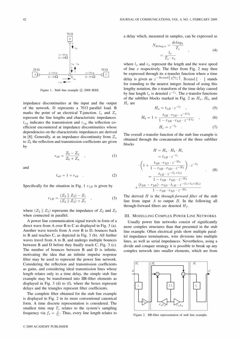
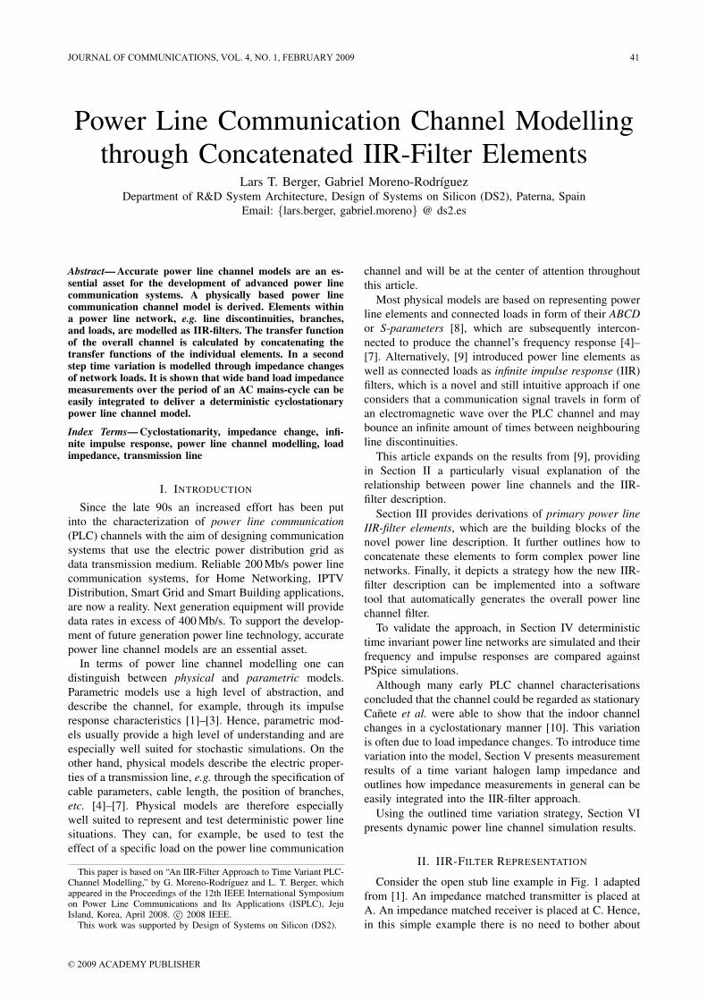
Figure 1. Stub line example c© 2008 IEEE.

impedance discontinuities at the input and the outputof the network. D represents a 70 Ω parallel load. Bmarks the point of an electrical T-junction. lx and Zx

represent the line lengths and characteristic impedances.txy indicates the transmission and rxy the reflection co-efficient encountered at impedance discontinuities whosedependencies on the characteristic impedances are derivedin [8]. Generally, at an impedance discontinuity from Za

to Zb the reflection and transmission coefficients are givenby

rab =Zb − Za

Zb + Za, (1)

and

tab = 1 + rab . (2)

Specifically for the situation in Fig. 1 r1B is given by

r1B =(Z2 ‖ Z3) − Z1

(Z2 ‖ Z3) + Z1, (3)

where (Z2 ‖ Z3) represents the impedance of Z2 and Z3

when connected in parallel.A power line communication signal travels in form of a

direct wave from A over B to C as displayed in Fig. 3 (a).Another wave travels from A over B to D, bounces backto B and reaches C, as depicted in Fig. 3 (b). All furtherwaves travel from A to B, and undergo multiple bouncesbetween B and D before they finally reach C, Fig. 3 (c).The number of bounces between B and D is infinite,motivating the idea that an infinite impulse responsefilter may be used to represent the power line network.Considering the reflection and transmission coefficientsas gains, and considering ideal transmission lines whoselength relates only to a time delay, the simple stub lineexample may be transformed into IIR-filter elements asdisplayed in Fig. 3 (d) to (f), where the boxes representdelays and the triangles represent filter coefficients.

The complete filter obtained for the stub line exampleis displayed in Fig. 2 in its more conventional canonicalform. A time discrete representation is considered. Thesmallest time step Ts relates to the system’s samplingfrequency via fs = 1

Ts. Thus, every line length relates to

a delay which, measured in samples, can be expressed as

Ndelay,x =delayx

Ts

=lx

Ts · vx

, (4)

where lx and vx represent the length and the wave speedof line x respectively. The filter from Fig. 2 may thenbe expressed through its z-transfer function where a timedelay is given as z−Round lx

Ts·vx. Round · stands

for rounding to the nearest integer. Instead of using thislengthy notation, the z-transform of the time delay causedby line length lx is denoted z−lx . The z-transfer functionsof the subfilter blocks marked in Fig. 2 as Ha, Hb, andHc are

Ha = t1B · z−l1 , (5)

Hb = 1 +t3B · r3D · z−2·l3

1 − r3B · r3D · z−2·l3 , (6)

Hc = z−l2 . (7)

The overall z-transfer function of the stub line example isobtained through the concatenation of the three subfilterblocks

H = Ha · Hb · Hc

= t1B · z−l1

·(

1 +t3B · r3D · z−2l3

1 − r3B · r3D · z−2l3

)· z−l2

=t1B · z−(l1+l2)

1 − r3B · r3D · z−2l3

+(t3B − r3B) · r3D · t1B · z−(l1+l2+2l3)

1 − r3B · r3D · z−2l3

. (8)

The derived H is the through-forward filter of the stubline from input A to output B. In the following allthrough-forward filters are denoted Hf .

III. MODELLING COMPLEX POWER LINE NETWORKS

Usually power line networks consist of significantlymore complex structures than that presented in the stubline example. Often electrical grids show multiple paral-lel impedance terminations, wire divisions into multiplelines, as well as serial impedances. Nevertheless, using adivide and conquer strategy it is possible to break up anycomplex network into smaller elements, which are from

Figure 2. IIR-filter representation of stub line example.

42 JOURNAL OF COMMUNICATIONS, VOL. 4, NO. 1, FEBRUARY 2009


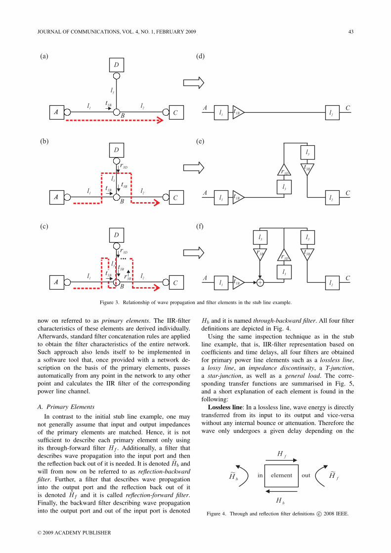
Figure 3. Relationship of wave propagation and filter elements in the stub line example.

now on referred to as primary elements. The IIR-filtercharacteristics of these elements are derived individually.Afterwards, standard filter concatenation rules are appliedto obtain the filter characteristics of the entire network.Such approach also lends itself to be implemented ina software tool that, once provided with a network de-scription on the basis of the primary elements, passesautomatically from any point in the network to any otherpoint and calculates the IIR filter of the correspondingpower line channel.

A. Primary ElementsIn contrast to the initial stub line example, one may

not generally assume that input and output impedancesof the primary elements are matched. Hence, it is notsufficient to describe each primary element only usingits through-forward filter Hf . Additionally, a filter thatdescribes wave propagation into the input port and thenthe reflection back out of it is needed. It is denoted Hb andwill from now on be referred to as reflection-backwardfilter. Further, a filter that describes wave propagationinto the output port and the reflection back out of itis denoted Hf and it is called reflection-forward filter.Finally, the backward filter describing wave propagationinto the output port and out of the input port is denoted

Hb and it is named through-backward filter. All four filterdefinitions are depicted in Fig. 4.

Using the same inspection technique as in the stubline example, that is, IIR-filter representation based oncoefficients and time delays, all four filters are obtainedfor primary power line elements such as a lossless line,a lossy line, an impedance discontinuity, a T-junction,a star-junction, as well as a general load. The corre-sponding transfer functions are summarised in Fig. 5,and a short explanation of each element is found in thefollowing:

Lossless line: In a lossless line, wave energy is directlytransferred from its input to its output and vice-versawithout any internal bounce or attenuation. Therefore thewave only undergoes a given delay depending on the

Figure 4. Through and reflection filter definitions c© 2008 IEEE.



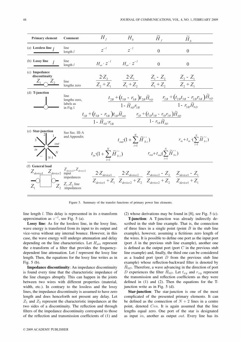
Figure 5. Summary of the transfer functions of primary power line elements.

line length l. This delay is represented in its z-transformapproximation as z−l, see Fig. 5 (a).

Lossy line: As for the lossless line, in the lossy line,wave energy is transferred from its input to its output andvice-versa without any internal bounce. However, in thiscase, the wave energy will undergo attenuation and delaydepending on the line characteristics. Let Hatt representthe z-transform of a filter that provides the frequency-dependent line attenuation. Let l represent the lossy linelength. Then, the equations for the lossy line writes as inFig. 5 (b).

Impedance discontinuity: An impedance discontinuityis found every time that the characteristic impedance ofthe line changes abruptly. This can happen in the jointsbetween two wires with different properties (material,width, etc.). In contrary to the lossless and the lossylines, the impedance discontinuity is assumed to have zerolength and does henceforth not present any delay. LetZ1 and Z2 represent the characteristic impedances at thetwo sides of a discontinuity. The reflection and throughfilters of the impedance discontinuity correspond to thoseof the reflection and transmission coefficients of (1) and

(2) whose derivations may be found in [8], see Fig. 5 (c).T-junction: A T-junction was already indirectly de-

scribed in the stub line example. That is, the connectionof three lines in a single point (point B in the stub lineexample), however, assuming a fictitious zero length ofthe wires. It is possible to define one port as the input port(port A in the previous stub line example), another oneis defined as the output port (port C in the previous stubline example) and, finally, the third one can be consideredas a loaded port (port D from the previous stub lineexample) whose reflection-backward filter is denoted byHbD. Therefore, a wave advancing in the direction of portD experiences the filter HbD. Let txy and rxy representthe transmission and reflection coefficients as they weredefined in (1) and (2). Then the equations for the T-junction write as in Fig. 5 (d).

Star-junction: The star-junction is one of the mostcomplicated of the presented primary elements. It canbe defined as the connection of N + 2 lines in a centrepoint, denoted Cen. It is again assumed that the linelengths equal zero. One port of the star is designatedas input in, another as output out. Every line has its



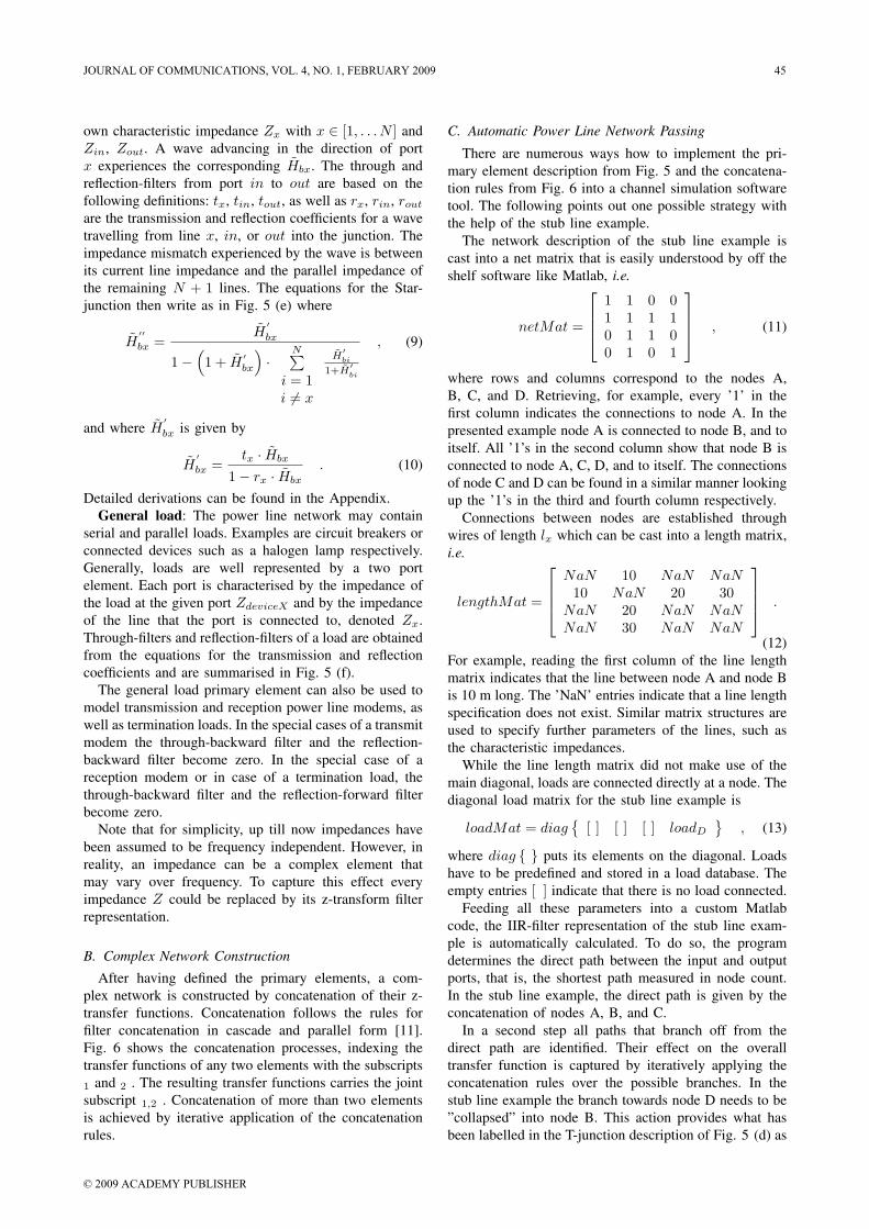
own characteristic impedance Zx with x ∈ [1, . . . N ] andZin, Zout. A wave advancing in the direction of portx experiences the corresponding Hbx. The through andreflection-filters from port in to out are based on thefollowing definitions: tx, tin, tout, as well as rx, rin, rout

are the transmission and reflection coefficients for a wavetravelling from line x, in, or out into the junction. Theimpedance mismatch experienced by the wave is betweenits current line impedance and the parallel impedance ofthe remaining N + 1 lines. The equations for the Star-junction then write as in Fig. 5 (e) where

H′′bx =

H′bx

1 −(1 + H

′bx

)·

N∑i = 1i = x

H′bi

1+H′bi

, (9)

and where H′bx is given by

H′bx =

tx · Hbx

1 − rx · Hbx

. (10)

Detailed derivations can be found in the Appendix.General load: The power line network may contain

serial and parallel loads. Examples are circuit breakers orconnected devices such as a halogen lamp respectively.Generally, loads are well represented by a two portelement. Each port is characterised by the impedance ofthe load at the given port ZdeviceX and by the impedanceof the line that the port is connected to, denoted Zx.Through-filters and reflection-filters of a load are obtainedfrom the equations for the transmission and reflectioncoefficients and are summarised in Fig. 5 (f).

The general load primary element can also be used tomodel transmission and reception power line modems, aswell as termination loads. In the special cases of a transmitmodem the through-backward filter and the reflection-backward filter become zero. In the special case of areception modem or in case of a termination load, thethrough-backward filter and the reflection-forward filterbecome zero.

Note that for simplicity, up till now impedances havebeen assumed to be frequency independent. However, inreality, an impedance can be a complex element thatmay vary over frequency. To capture this effect everyimpedance Z could be replaced by its z-transform filterrepresentation.

B. Complex Network Construction

After having defined the primary elements, a com-plex network is constructed by concatenation of their z-transfer functions. Concatenation follows the rules forfilter concatenation in cascade and parallel form [11].Fig. 6 shows the concatenation processes, indexing thetransfer functions of any two elements with the subscripts1 and 2 . The resulting transfer functions carries the jointsubscript 1,2 . Concatenation of more than two elementsis achieved by iterative application of the concatenationrules.

C. Automatic Power Line Network Passing

There are numerous ways how to implement the pri-mary element description from Fig. 5 and the concatena-tion rules from Fig. 6 into a channel simulation softwaretool. The following points out one possible strategy withthe help of the stub line example.

The network description of the stub line example iscast into a net matrix that is easily understood by off theshelf software like Matlab, i.e.

netMat =

⎡⎢⎢⎣

1 1 0 01 1 1 10 1 1 00 1 0 1

⎤⎥⎥⎦ , (11)

where rows and columns correspond to the nodes A,B, C, and D. Retrieving, for example, every ’1’ in thefirst column indicates the connections to node A. In thepresented example node A is connected to node B, and toitself. All ’1’s in the second column show that node B isconnected to node A, C, D, and to itself. The connectionsof node C and D can be found in a similar manner lookingup the ’1’s in the third and fourth column respectively.

Connections between nodes are established throughwires of length lx which can be cast into a length matrix,i.e.

lengthMat =

⎡⎢⎢⎣

NaN 10 NaN NaN10 NaN 20 30

NaN 20 NaN NaNNaN 30 NaN NaN

⎤⎥⎥⎦ .

(12)For example, reading the first column of the line lengthmatrix indicates that the line between node A and node Bis 10 m long. The ’NaN’ entries indicate that a line lengthspecification does not exist. Similar matrix structures areused to specify further parameters of the lines, such asthe characteristic impedances.

While the line length matrix did not make use of themain diagonal, loads are connected directly at a node. Thediagonal load matrix for the stub line example is

loadMat = diag

[ ] [ ] [ ] loadD

, (13)

where diag puts its elements on the diagonal. Loadshave to be predefined and stored in a load database. Theempty entries [ ] indicate that there is no load connected.

Feeding all these parameters into a custom Matlabcode, the IIR-filter representation of the stub line exam-ple is automatically calculated. To do so, the programdetermines the direct path between the input and outputports, that is, the shortest path measured in node count.In the stub line example, the direct path is given by theconcatenation of nodes A, B, and C.

In a second step all paths that branch off from thedirect path are identified. Their effect on the overalltransfer function is captured by iteratively applying theconcatenation rules over the possible branches. In thestub line example the branch towards node D needs to be”collapsed” into node B. This action provides what hasbeen labelled in the T-junction description of Fig. 5 (d) as



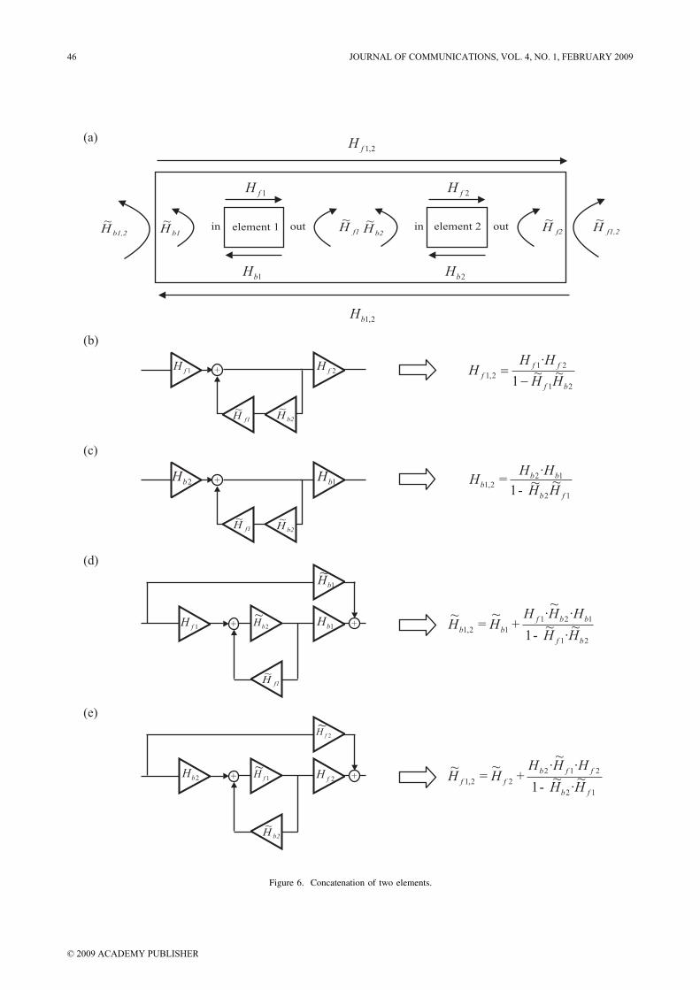
Figure 6. Concatenation of two elements.



Figure 7. Complex power line network example c© 2008 IEEE.

HbD. To use the the concatenation rules defined in Fig. 6the lossless line of length l3 is associated with element 1.Further, load D is associated with element 2. HbD is thenobtained through application of the equation in Fig. 6 (d)

HbD = Hb1,2

= 0 +z−l3 · r3D · z−l3

1 − 0 · r3D

= r3D · z−2l3

, (14)

where it is used that the reflection-backward filter ofelement 1, i.e. Hb1 is zero.

In more complex networks iterative application of theconcatenation rules from Fig. 6 is required to collapse allbranch effects onto the direct path.

The final step is to role up the network from the receivertowards the transmitter, ”collapsing” step by step thefilters on the direct path into a single filter. In the stub lineexample, three elements have to be collapsed to obtain theoverall transfer function. (i) The lossless line of length l1which will be indexed with α. (ii) The T-junction locatedat node B that already includes the effect of the branchtowards D which will be indexed with β. (iii) The losslessline of length l2 which will be indexed by γ.

The calculation of the through-forward filter for theconcatenation of element β with element γ is given bythe equation in Fig. 6 (b). Taking into account (14) andthat the reflection-backwards filter for a lossless line iszero, it writes

Hf β,γ

∣∣∣Hbγ=0 = Hf β · Hf γ

=t1B + (t3B − r3B) · t1B · r3D · z−2l3

1 − r3D · z−2l3 · r3B· z−l2

. (15)

Finally, the resulting filter is calculated by the con-catenation of α with the previous joint element β, γ.

Figure 8. Time variation by switching through different linear timeinvariant filters.

Taking into account that the reflection-forward filter forthe lossless line is zero it writes

Hf α,β,γ

∣∣∣Hf1=0 = Hf α · Hf β,γ

= z−l1 · t1B + (t3B − r3B) · t1B · r3D · z−2l3

1 − r3D · z−2l3 · r3B· z−l2

,

(16)

which is equivalent to (8).Propagation scenarios can either be defined in a deter-

ministic or a stochastic manner. The stochastic represen-tation of a scenario can be achieved by the generation ofthe net, length and load matrices following given distri-bution probabilities. Besides, in multi modem scenarios,where several input and output ports are defined, mostof the subcalculation results can be reused to obtain theoverall transfer functions for every input output pair, thusreducing the computational effort.

IV. STATIC IIR-FILTER MODEL VALIDATION

Consider the simple stub line example from Fig. 1 aswell as a more complex power line network exampledisplayed in Fig. 7. To validate the IIR-filter based mod-elling strategy, IIR-filter and PSpice implementations ofthe networks have been obtained using common resistors,voltage source and transmission lines provided in PSpicelibraries. The PSpice frequency transfer function was ob-tained with an AC-Sweep, while the impulse response wasobtained by exciting with a voltage impulse that approxi-mates a delta function. As it does not reassemble an idealdelta with unit energy the PSpice impulse response wasafterwards power normalised. The corresponding resultsare compared in Fig. 10. It can be seen that a good matchis obtained in all cases which underlines the validity ofthe IIR-filter approach.

V. DYNAMIC IIR-FILTER MODELS BASED ON LOADREFLECTION COEFFICIENT MEASUREMENTS

Till now the aspect of time dynamics has been ne-glected. However, loads, such as a halogen lamp con-nected to the electrical grid, change their input impedancesynchronously as a function of the AC-mains cycle,causing cyclostationary repetitions [10], [12], [13]. To

Figure 9. Wideband halogen lamp reflection coefficient measurementsduring three different points in an AC mains-cycle c© 2008 IEEE.



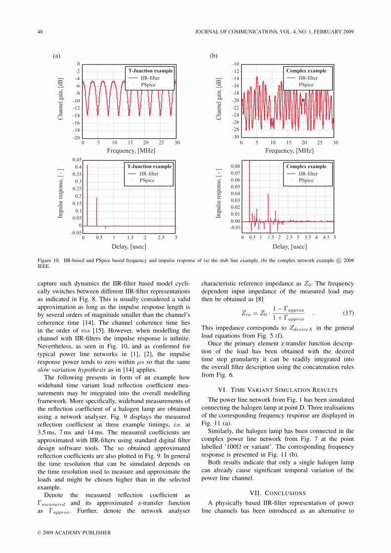
Figure 10. IIR-based and PSpice based frequency and impulse response of (a) the stub line example, (b) the complex network example c© 2008IEEE.

capture such dynamics the IIR-filter based model cycli-cally switches between different IIR-filter representationsas indicated in Fig. 8. This is usually considered a validapproximation as long as the impulse response length isby several orders of magnitude smaller than the channel’scoherence time [14]. The channel coherence time liesin the order of ms [15]. However, when modelling thechannel with IIR-filters the impulse response is infinite.Nevertheless, as seen in Fig. 10, and as confirmed fortypical power line networks in [1], [2], the impulseresponse power tends to zero within µs so that the sameslow variation hypothesis as in [14] applies.

The following presents in form of an example howwideband time variant load reflection coefficient mea-surements may be integrated into the overall modellingframework. More specifically, wideband measurements ofthe reflection coefficient of a halogen lamp are obtainedusing a network analyser. Fig. 9 displays the measuredreflection coefficient at three example timings, i.e. at3.5 ms, 7 ms and 14 ms. The measured coefficients areapproximated with IIR-filters using standard digital filterdesign software tools. The so obtained approximatedreflection coefficients are also plotted in Fig. 9. In generalthe time resolution that can be simulated depends onthe time resolution used to measure and approximate theloads and might be chosen higher than in the selectedexample.

Denote the measured reflection coefficient asΓmeasured and its approximated z-transfer functionas Γapprox. Further, denote the network analyser

characteristic reference impedance as Z0. The frequencydependent input impedance of the measured load maythen be obtained as [8]

Zin = Z0 · 1 − Γapprox

1 + Γapprox. (17)

This impedance corresponds to ZdeviceX in the generalload equations from Fig. 5 (f).

Once the primary element z-transfer function descrip-tion of the load has been obtained with the desiredtime step granularity it can be readily integrated intothe overall filter description using the concatenation rulesfrom Fig. 6.

VI. TIME VARIANT SIMULATION RESULTS

The power line network from Fig. 1 has been simulatedconnecting the halogen lamp at point D. Three realisationsof the corresponding frequency response are displayed inFig. 11 (a).

Similarly, the halogen lamp has been connected in thecomplex power line network from Fig. 7 at the pointlabelled ’100Ω or variant’. The corresponding frequencyresponse is presented in Fig. 11 (b).

Both results indicate that only a single halogen lampcan already cause significant temporal variation of thepower line channel.

VII. CONCLUSIONS

A physically based IIR-filter representation of powerline channels has been introduced as an alternative to



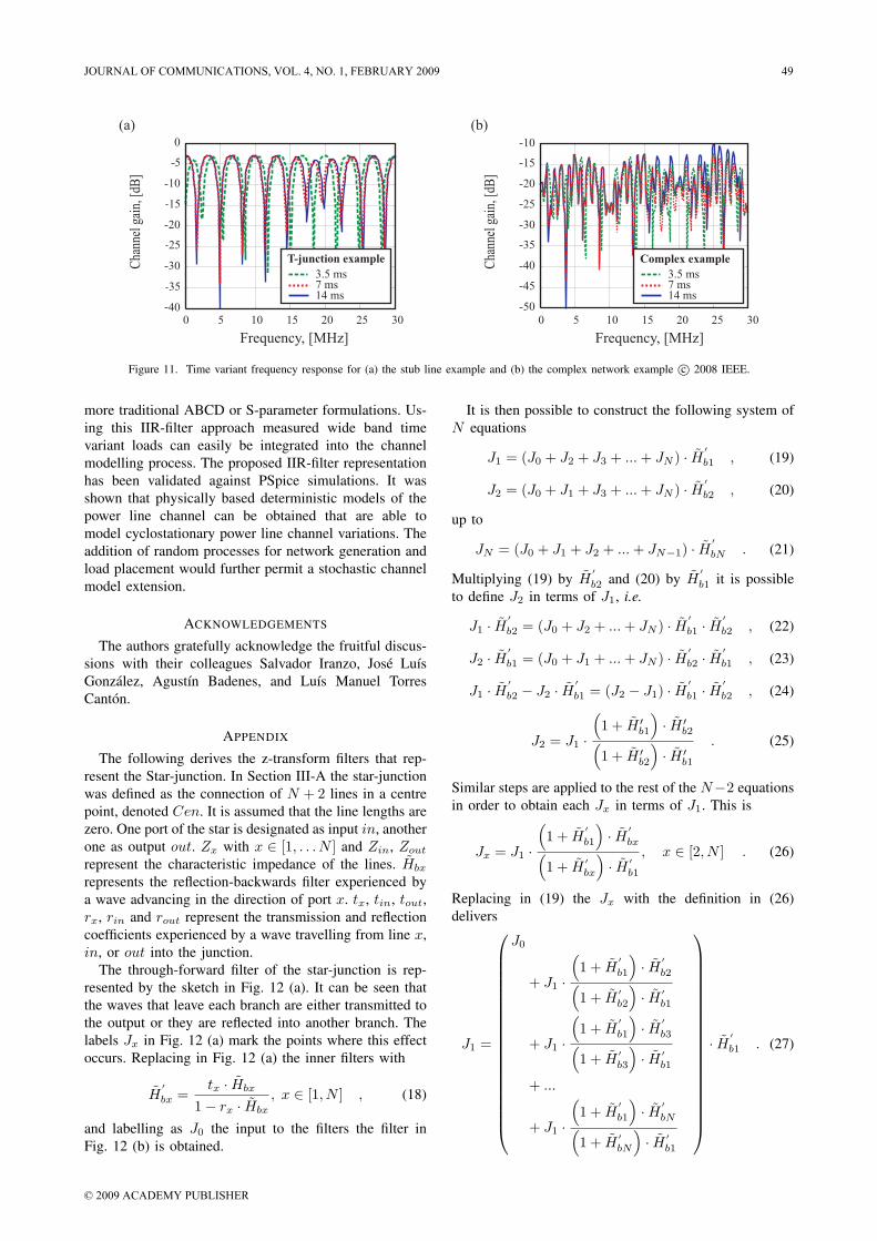
Figure 11. Time variant frequency response for (a) the stub line example and (b) the complex network example c© 2008 IEEE.

more traditional ABCD or S-parameter formulations. Us-ing this IIR-filter approach measured wide band timevariant loads can easily be integrated into the channelmodelling process. The proposed IIR-filter representationhas been validated against PSpice simulations. It wasshown that physically based deterministic models of thepower line channel can be obtained that are able tomodel cyclostationary power line channel variations. Theaddition of random processes for network generation andload placement would further permit a stochastic channelmodel extension.

ACKNOWLEDGEMENTS

The authors gratefully acknowledge the fruitful discus-sions with their colleagues Salvador Iranzo, Jose LuısGonzalez, Agustın Badenes, and Luıs Manuel TorresCanton.

APPENDIX

The following derives the z-transform filters that rep-resent the Star-junction. In Section III-A the star-junctionwas defined as the connection of N + 2 lines in a centrepoint, denoted Cen. It is assumed that the line lengths arezero. One port of the star is designated as input in, anotherone as output out. Zx with x ∈ [1, . . . N ] and Zin, Zout

represent the characteristic impedance of the lines. Hbx

represents the reflection-backwards filter experienced bya wave advancing in the direction of port x. tx, tin, tout,rx, rin and rout represent the transmission and reflectioncoefficients experienced by a wave travelling from line x,in, or out into the junction.

The through-forward filter of the star-junction is rep-resented by the sketch in Fig. 12 (a). It can be seen thatthe waves that leave each branch are either transmitted tothe output or they are reflected into another branch. Thelabels Jx in Fig. 12 (a) mark the points where this effectoccurs. Replacing in Fig. 12 (a) the inner filters with

H′bx =

tx · Hbx

1 − rx · Hbx

, x ∈ [1, N ] , (18)

and labelling as J0 the input to the filters the filter inFig. 12 (b) is obtained.

It is then possible to construct the following system ofN equations

J1 = (J0 + J2 + J3 + ... + JN ) · H ′b1 , (19)

J2 = (J0 + J1 + J3 + ... + JN ) · H ′b2 , (20)

up to

JN = (J0 + J1 + J2 + ... + JN−1) · H ′bN . (21)

Multiplying (19) by H′b2 and (20) by H

′b1 it is possible

to define J2 in terms of J1, i.e.

J1 · H ′b2 = (J0 + J2 + ... + JN ) · H ′

b1 · H′b2 , (22)

J2 · H ′b1 = (J0 + J1 + ... + JN ) · H ′

b2 · H′b1 , (23)

J1 · H ′b2 − J2 · H ′

b1 = (J2 − J1) · H ′b1 · H

′b2 , (24)

J2 = J1 ·(1 + H ′

b1

)· H ′

b2(1 + H ′

b2

)· H ′

b1

. (25)

Similar steps are applied to the rest of the N−2 equationsin order to obtain each Jx in terms of J1. This is

Jx = J1 ·(1 + H

′b1

)· H ′

bx(1 + H

′bx

)· H ′

b1

, x ∈ [2, N ] . (26)

Replacing in (19) the Jx with the definition in (26)delivers

J1 =

⎛⎜⎜⎜⎜⎜⎜⎜⎜⎜⎜⎜⎜⎜⎜⎜⎜⎜⎜⎜⎝

J0

+ J1 ·(1 + H

′b1

)· H ′

b2(1 + H

′b2

)· H ′

b1

+ J1 ·(1 + H

′b1

)· H ′

b3(1 + H

′b3

)· H ′

b1

+ ...

+ J1 ·(1 + H

′b1

)· H ′

bN(1 + H

′bN

)· H ′

b1

⎞⎟⎟⎟⎟⎟⎟⎟⎟⎟⎟⎟⎟⎟⎟⎟⎟⎟⎟⎟⎠

· H ′b1 . (27)



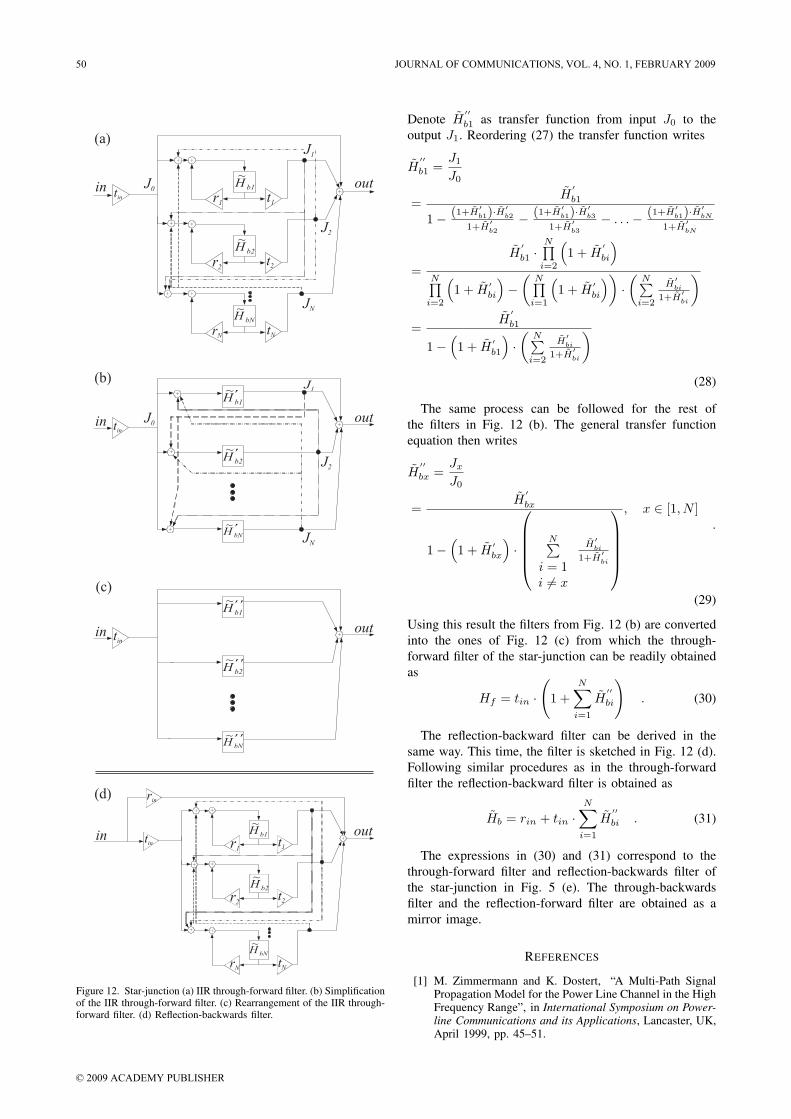
Figure 12. Star-junction (a) IIR through-forward filter. (b) Simplificationof the IIR through-forward filter. (c) Rearrangement of the IIR through-forward filter. (d) Reflection-backwards filter.

Denote H′′b1 as transfer function from input J0 to the

output J1. Reordering (27) the transfer function writes

H′′b1 =

J1

J0

=H

′b1

1 − (1+H′b1)·H

′b2

1+H′b2

− (1+H′b1)·H

′b3

1+H′b3

− . . . − (1+H′b1)·H

′bN

1+H′bN

=H

′b1 ·

N∏i=2

(1 + H

′bi

)N∏

i=2

(1 + H

′bi

)−(

N∏i=1

(1 + H

′bi

))·(

N∑i=2

H′bi

1+H′bi

)

=H

′b1

1 −(1 + H

′b1

)·(

N∑i=2

H′bi

1+H′bi

)

(28)

The same process can be followed for the rest ofthe filters in Fig. 12 (b). The general transfer functionequation then writes

H′′bx =

Jx

J0

=H

′bx

1 −(1 + H

′bx

)·

⎛⎜⎜⎜⎜⎝

N∑i = 1i = x

H′bi

1+H′bi

⎞⎟⎟⎟⎟⎠

, x ∈ [1, N ].

(29)

Using this result the filters from Fig. 12 (b) are convertedinto the ones of Fig. 12 (c) from which the through-forward filter of the star-junction can be readily obtainedas

Hf = tin ·(

1 +N∑

i=1

H′′bi

). (30)

The reflection-backward filter can be derived in thesame way. This time, the filter is sketched in Fig. 12 (d).Following similar procedures as in the through-forwardfilter the reflection-backward filter is obtained as

Hb = rin + tin ·N∑

i=1

H′′bi . (31)

The expressions in (30) and (31) correspond to thethrough-forward filter and reflection-backwards filter ofthe star-junction in Fig. 5 (e). The through-backwardsfilter and the reflection-forward filter are obtained as amirror image.

REFERENCES

[1] M. Zimmermann and K. Dostert, “A Multi-Path SignalPropagation Model for the Power Line Channel in the HighFrequency Range”, in International Symposium on Power-line Communications and its Applications, Lancaster, UK,April 1999, pp. 45–51.



[2] H. Philipps, “Development of a Statistical Model forPowerline Communication Channels”, in InternationalSymposium on Power Line Communications (ISPLC), Lim-erick, Ireland, April 2000, pp. 153–160.

[3] M. Babic, M. Hagenau, K. Dostert, and J. Bausch, “Theo-retical Postulation of PLC Channel Model”, IST IntegratedProject Deliverable D4v2.0, The OPERA Consortium,March 2005.

[4] T. Esmailian, F. R. Kschischang, and P. G. Gulak, “AnIn-building Power Line Channel Simulator”, in Interna-tional Symposium on Power Line Communications and ItsApplications (ISPLC), Athens, Greece, March 2002.

[5] S. Galli and T. Banwell, “A Novel Approach to theModeling of the Indoor Power Line Channel - Part II:Transfer Function and its Properties”, IEEE Transactionson Power Delivery, vol. 20, no. 3, pp. 1869 – 1878, July2005.

[6] T. Sartenaer and P. Delogne, “Deterministic Modelingof the (Shielded) Outdoor Power Line Channel based onthe Multiconductor Transmission Line Equations”, IEEEJournal on Selected Areas in Communications, vol. 24, no.7, pp. 1277–1291, July 2006.

[7] S. Barmada, A. Musolino, and M. Raugi, “Innova-tive Model for Time-Varying Power Line CommunicationChannel Response Evaluation”, IEEE Journal on SelectedAreas in Communications, vol. 7, no. 24, pp. 1317–1326,July 2006.

[8] D. M. Pozar, Microwave Engineering, John Wiley & Sons,Inc., 3rd edition, 2005.

[9] G. Moreno-Rodrıguez and L. T. Berger, “An IIR-filter Ap-proach to Time Variant PLC-Channel Modelling”, in IEEEInternational Symposium on Power Line Communicationsand Its Applications, Jeju, South Korea, April 2008, pp.87–92.

[10] F. J. Canete Corripio, J. A. Cortes Arrabal, L. Diez del Rio,and J. T. Entrambasaguas Munoz, “Analysis of the CyclicShort-Term Variation of Indoor Power Line Channels”,IEEE Journal on Selected Areas in Communications, vol.24, no. 7, pp. 1327 – 1338, July 2006.

[11] A. V. Oppenheim, R. W. Schafer, and J. R. Buck, Discrete-Time Signal Processing, Signal Processing Series. PrenticeHall, 2nd edition, 1999.

[12] F. J. Canete, L. Dıez, J. A. Cortes, and J. T. Entram-basaguas, “Broadband modelling of indoor power-linechannels”, IEEE Transactions on Consumer Electronics,vol. 48, no. 1, pp. 175–183, February 2002.

[13] J. A. Cortes, F. J. Canete, L. Diez, and J. T. Entram-basaguas, “Characterization of the Cyclic Short-TimeVariation of Indoor Power-Line Channels Response”, inInternational Symposium on Power Line Communicationsand Its Applications (ISPLC), Vancouver, Canada, April2005, pp. 326–330.

[14] S. Sancha, F. J. Canete, L. Diez, and J. T. Entrambasaguas,“A Channel Simulator for Indoor Power-line Communica-tions”, in IEEE International Symposium on Power LineCommunications and Its Applications, Pisa, Italy, March2007, pp. 104–109.

[15] S. Katar, B. Mashburn, K. Afkhamie, H. Latchman, andR. Newman, “Channel Adaptation based on Cyclo-Stationary Noise Characteristics in PLC Systems”, in IEEEInternational Symposium on Power Line Communicationsand Its Applications, March 2006, pp. 16–21.

Lars Torsten Berger received the Dipl.-Ing. degree in electricalengineering, the M.Sc. degree in communication systems andsignal processing, and the Ph.D. degree in wireless communica-tions from the University of Cooperative Education Ravensburg(Germany), the University of Bristol (United Kingdom), and

Aalborg University (Denmark) in 1999, 2001 and 2005 respec-tively.

After having worked for DaimlerChrysler/Dornier (Germany,1996 to 1999), and Nortel Networks (United Kingdom, 2000to 2001), he joint the Cellular Systems Research Group (CSys)at Aalborg University. There his work, financed by Nokia Net-works, focussed on the evaluation of multi-antenna processingalgorithms. From 2005 to 2006 he was a Visiting Professor atthe University Carlos III of Madrid (Spain), teaching land andsatellite radio communications. At the same time, he worked onseveral international projects in the areas of 4G system architec-ture development and wireless sensor networks. Since 2006 he isa Senior Engineer at the System Architecture R&D Departmentof Design of Systems on Silicon (DS2), focussing on physicallayer power line communication system development.

Dr. Berger is a member of the IEEE. He has served asTPC member for the International Wireless Communications &Mobile Computing Conference (IWCMC 2006), and is regu-larly reviewing contributions for international conferences andJournals such as the IEEE Communications Letters, or the IEEETransactions on Signal Processing.

Gabriel Moreno Rodrıguez was born in Requena, Spain, in1981. He received the M. Sc. degree in Telecommunications En-gineering from the Universidad Politecnica de Valencia (UPV),Spain, in 2005.

In 2004, he joined Telefonica R&D, Madrid, where he workedin GMPLS/ASON optical networks. In 2006, he joined Designof Systems on Silicon (DS2) where he is currently working asSystems Engineer in the System Architecture R&D Department.His research interests include signal processing, as well aschannel and noise modelling in power line networks.

Mr. Moreno received the Best Thesis of the Year 2005/2006Award on Security Systems by the Spanish TelecommunicationsCommittee, which was based on research he undertook duringa one year stay at the University of New South Wales, Sydney,Australia.



Power Line Communication Channel Modelling through ... · Power Line Communication Channel...

Documents

Transcript of Power Line Communication Channel Modelling through ... · Power Line Communication Channel...