
On Advanced Channel Modelling for Network Planning
154
UNIVERSITY OF SHEFFIELD On Advanced Channel Modelling for Network Planning by Jialai Weng Faculty of Engineering Department of Electronic and Electrical Engineering October 2017
Transcript of On Advanced Channel Modelling for Network Planning

UNIVERSITY OF SHEFFIELD
On Advanced Channel Modelling forNetwork Planning
by
Jialai Weng
Faculty of EngineeringDepartment of Electronic and Electrical Engineering
October 2017

Declaration of Authorship
Part of the work included in this thesis has been published in the following publications:
2015 An Averaging Path Loss Prediction Model Based on Ray Tracing (Jialai Weng,
Cong Wang, Jie Zhang) Accepted In ZTE Communications
2015 A Mathematical Formulation for Channel Map and Its Application in MIMO
Systems (Jialai Weng, Wuling Liu, Haonan Hu, Xiaoli Chu, Jie Zhang) In Antennas
and Propagation Conference (LAPC), 2015 Loughborough
2015 A Simulation Based Distributed MIMO Network Optimisation Using Chan-
nel Map (Jialai Weng, Jonathan M. Rigelsford, and J. Zhang) PIERS (Progress In
Electromagnetics Research Symposium), Prague, Czech Republic, July 2015.
2015 Modelling the mmWave Channel Based on Intelligent Ray Launching Model
(Jialai Weng, Xiaoming Tu, Zhihua Lai, Jie Zhang), In Antennas and Propagation
(EUCAP), Proceedings of the 9th European Conference on, April, 2015.
2014 Indoor Massive MIMO Channel Modelling Using Ray-Launching Simulation
(Jialai Weng, Xiaoming Tu, Zhihua Lai, Sana Salous, Jie Zhang), In International
Journal of Antennas and Propagation, 2014
2014 Capacity Field: Modelling Channel Capacity from Electromagnetic Propagation
Perspective (Jialai Weng, Xiaoming Tu, Jie Zhang), In Antennas and Propagation
(EUCAP), Proceedings of the 8th European Conference on, 2014.
The rest part of the work during my PhD has not been included in this thesis. They are
in preparation to be published or have been published as:
2015 Wireless Channel Capacity from Electromagnetic Perspective (Jialai Weng)In
Preparation
2015 The Impact of Propagation Mechanisms on Wireless Channel Capacity (Jialai
Weng)In Preparation
2015 An Averaging Path Loss Prediction Model Based on Ray Tracing (Jialai Weng,
Jie Zhang) In Press
i

ii
2015 Coverage Performance Analysis of FeICIC Low Power Subframes (Haonan Hu,
Jialai Weng, Jie Zhang), submitted to IEEE Transaction on Wireless Communica-
tions, Accepted
2015 How Densely Should Wireless Networks be Deployed? (Jialai Weng, Haonan
Hu, Jie Zhang)In The University of Sheffield Engineering Symposium (USES) 2015,
June, 2015
2015 A Network Deployment Strategy for Home Area Networks in Smart Grid (De-
hua Li, Jialai Weng, Xiaoli Chu, Jie Zhang) 2015 IEEE 25th International Symposium
on Personal, Indoor and Mobile Radio Communications - (PIMRC)
2014 On the Use of an Intelligent Ray Launching in MIMO channel Modelling for
Network Planning (Xiaoming Tu, Jialai Weng, S. Salas, Jie Zhang), In General
Assembly and Scientific Symposium (URSI GASS), 2014 XXXIth URSI, pp. 1-4, 2014.
2013 A Dual-Polarisation Modelling Method for Simulation-based Propagation Mod-
els (Jialai Weng, Zhihua Lai, Jie Zhang), In Antennas and Propagation Conference
(LAPC), 2013 Loughborough, pp. 436-440, 2013.
2013 Realistic Prediction of BER and AMC with MRC Diversity for Indoor Wireless
Transmissions (Meiling Luo, G. Villemaud, Jialai Weng, J.-M. Gorce, Jie Zhang),
In Wireless Communications and Networking Conference (WCNC), 2013 IEEE, pp.
4059-4064, 2013.
2011 Channel Measurement and Characterization of Interference Between Residen-
tial Femto-cell Systems (Xiang Gao, A. Alayon Glazunov, Jialai Weng, Cheng
Fang, Jie Zhang, F. Tufvesson), In Antennas and Propagation (EUCAP), Proceedings
of the 5th European Conference on, pp. 3769-3773, 2011.
UNIVERSITY OF SHEFFIELD
AbstractFaculty of Engineering
Department of Electronic and Electrical Engineering
by Jialai Weng
With the increasing demand for high speed wireless network services, the next genera-
tion wireless networks are proposed to use advanced wireless communication technolo-
gies. These technologies include massive MIMO, mmWave and distributed MIMO. In
order to deploy wireless networks equipped with these technologies, channel models
capturing the channel features and characteristics of these wireless technologies are es-
sential in the planning and optimisation of networks. However, conventional channel
models lack the capability to support these next generation network technologies. In
this PhD thesis, I investigated the channel models for the next generation wireless tech-
nologies, including massive MIMO, mmWave communications and distributed MIMO.
I developed channel models for network planning and optimisation based on conven-
tional ray launching algorithms for these wireless technologies. The models have been
validated and applied to optimise network performance. The existing challenge in
wireless channel modelling is the improvement of modelling accuracy without increas-
ing modelling complexity. In order to achieve this goal, a new calibration method is
developed to improve the accuracy of the predication model when measurements are
available. Moreover, in order to use the channel models as an effective tool in wire-
less network planning and optimisation, a new wireless capacity definition from radio
propagation perspective is also investigated. It provides insight to the physical limit of
wireless channel capacity from a radio propagation perspective.

Acknowledgements
First, I would like to thank my PhD supervisor Prof. Jie Zhang. He helped me to
choose the research project on channel modelling. Through the PhD research project,
his support and advice inspired many interesting research discussion and exploration.
Without his help and guidance, this thesis would be impossible.
Second, I would like to thank the thesis examiners, Prof. Sana Salous and Dr. Jonathan
Rigelsford for their meticulous review and valuable comments to the first submission of
this thesis. Their review and feedback significantly improved the quality of this thesis.
Third, I would like to thank many colleagues from the Communication Research Group:
Dr. Xiaoli Chu, Mr. Wuling Liu, Mr. Dehua Li, Mr. Haonan Hu, Mr. Yue Wu, Mr. Ran
Tao, Mr. Qi Hong and Miss Hui Zheng. Thank you! It is a lovely experience to work
with you in the communication group. Thank you for all the discussions and help!
I would also like to thank my collaborators at Ranplan Wireless Network Design: Dr.
Zhihua Lai, Mr. Xiaoming Tu and Mr. Hanye Hu. Thank you for your help!
Last but not least, I would like to thank Prof. Sana Salous at Durham University
for hosting me as a visiting PhD student in 2013 to 2014 and offering me research
opportunity to work on channel measurement.
iv

Contents
Declaration of Authorship i
Abstract iii
Acknowledgements iv
List of Figures viii
List of Tables x
Abbreviations xi
1 Background and Research Problems 11.1 Introduction . . . . . . . . . . . . . . . . . . . . . . . . . . . . . . . . . . . 11.2 Background . . . . . . . . . . . . . . . . . . . . . . . . . . . . . . . . . . . 2
1.2.1 Wireless Network Planning . . . . . . . . . . . . . . . . . . . . . . 31.2.2 Channel Modelling for Network Planning . . . . . . . . . . . . . 71.2.3 Ray Optics for Radio Propagation Prediction: A Brief History . . 8
1.3 Challenges . . . . . . . . . . . . . . . . . . . . . . . . . . . . . . . . . . . . 101.3.1 Massive MIMO Channel Models . . . . . . . . . . . . . . . . . . . 101.3.2 Millimetre Wave Channel Models . . . . . . . . . . . . . . . . . . 121.3.3 Distributed MIMO . . . . . . . . . . . . . . . . . . . . . . . . . . . 131.3.4 Hybrid Propagation Model . . . . . . . . . . . . . . . . . . . . . . 141.3.5 Capacity from Electromagnetic Perspective . . . . . . . . . . . . . 15
1.4 Contributions . . . . . . . . . . . . . . . . . . . . . . . . . . . . . . . . . . 161.4.1 Massive MIMO . . . . . . . . . . . . . . . . . . . . . . . . . . . . . 161.4.2 mmWave Channel . . . . . . . . . . . . . . . . . . . . . . . . . . . 171.4.3 Distributed MIMO . . . . . . . . . . . . . . . . . . . . . . . . . . . 171.4.4 Channel Model Calibration . . . . . . . . . . . . . . . . . . . . . . 171.4.5 Channel Capacity from Electromagnetic Perspective . . . . . . . 18
1.5 Thesis Overview . . . . . . . . . . . . . . . . . . . . . . . . . . . . . . . . 18
2 Indoor Massive MIMO Channel Modelling using Ray Launching 192.1 Introduction . . . . . . . . . . . . . . . . . . . . . . . . . . . . . . . . . . . 192.2 MIMO Modelling using Ray Launching . . . . . . . . . . . . . . . . . . . 22
2.2.1 Model 1: Deterministic Ray-Launching Model for Massive MIMO 22
v

Contents vi
2.2.2 Model 2: Ray-Launching Based Deterministic Phase-shift Modelfor Massive MIMO . . . . . . . . . . . . . . . . . . . . . . . . . . . 25
2.2.3 Model 3: Ray-Launching Based Probabilistic Model for MassiveMIMO . . . . . . . . . . . . . . . . . . . . . . . . . . . . . . . . . . 29
2.2.4 Model 4: Simplified Ray-Launching Based Probabilistic Modelfor Massive MIMO . . . . . . . . . . . . . . . . . . . . . . . . . . . 31
2.3 Measurement Campaigns . . . . . . . . . . . . . . . . . . . . . . . . . . . 322.3.1 Measurement of Downlink Channel . . . . . . . . . . . . . . . . . 322.3.2 Measurement of Uplink Channel . . . . . . . . . . . . . . . . . . . 34
2.4 Measurement and Simulation Comparison and Analysis . . . . . . . . . 362.4.1 Computational Efficiency . . . . . . . . . . . . . . . . . . . . . . . 362.4.2 Received signal power . . . . . . . . . . . . . . . . . . . . . . . . . 372.4.3 Distribution of Channel Elements . . . . . . . . . . . . . . . . . . 392.4.4 Channel Capacity Results . . . . . . . . . . . . . . . . . . . . . . . 40
2.5 Conclusion . . . . . . . . . . . . . . . . . . . . . . . . . . . . . . . . . . . . 41
3 Ray Launching based mmWave Channel Modelling for Indoor Propagation 433.1 Introduction . . . . . . . . . . . . . . . . . . . . . . . . . . . . . . . . . . . 433.2 The Path Loss Model based on Ray Launching . . . . . . . . . . . . . . . 443.3 Channel Measurement . . . . . . . . . . . . . . . . . . . . . . . . . . . . . 493.4 Simulation Results and Comparison . . . . . . . . . . . . . . . . . . . . . 503.5 Conclusion . . . . . . . . . . . . . . . . . . . . . . . . . . . . . . . . . . . . 52
4 A Vector MIMO Channel Map Construction and Its Applications 544.1 Introduction . . . . . . . . . . . . . . . . . . . . . . . . . . . . . . . . . . . 544.2 Mathematical Formulation of Channel Map . . . . . . . . . . . . . . . . . 57
4.2.1 Single Antenna Channel Map . . . . . . . . . . . . . . . . . . . . . 574.2.2 MIMO channel map . . . . . . . . . . . . . . . . . . . . . . . . . . 59
4.3 Construction of MIMO channel map using distributed antenna systems 614.4 Numerical Examples . . . . . . . . . . . . . . . . . . . . . . . . . . . . . . 66
4.4.1 Channel Capacity Optimisation . . . . . . . . . . . . . . . . . . . . 694.4.2 Error Rate Optimisation . . . . . . . . . . . . . . . . . . . . . . . . 71
4.5 Conclusion . . . . . . . . . . . . . . . . . . . . . . . . . . . . . . . . . . . . 72
5 A Least Square Path Loss Model Calibration Method 745.1 Introduction . . . . . . . . . . . . . . . . . . . . . . . . . . . . . . . . . . . 745.2 The Sum-and-Average Multipath Path Loss Model . . . . . . . . . . . . . 76
5.2.1 Background and Motivation . . . . . . . . . . . . . . . . . . . . . . 765.2.2 The Sum-and-Average Multipath Path Loss Model based on Ray
Launching . . . . . . . . . . . . . . . . . . . . . . . . . . . . . . . . 785.2.3 Theoretical Model Parameter Values . . . . . . . . . . . . . . . . . 795.2.4 Sum-and-Average Model with Various Materials . . . . . . . . . . 835.2.5 An Efficient Parameter Calibration Method for the Model . . . . 84
5.3 Simulation, Measurement and Calibration . . . . . . . . . . . . . . . . . . 865.3.1 Environment Description . . . . . . . . . . . . . . . . . . . . . . . 865.3.2 The Propagation Setting and Channel Measurement . . . . . . . . 865.3.3 Simulation Setting . . . . . . . . . . . . . . . . . . . . . . . . . . . 865.3.4 Simulation Results - Un-calibrated . . . . . . . . . . . . . . . . . . 88

Contents vii
5.3.5 Parameter Calibration . . . . . . . . . . . . . . . . . . . . . . . . . 885.3.6 Discussion and Analysis . . . . . . . . . . . . . . . . . . . . . . . . 90
5.4 Conclusion . . . . . . . . . . . . . . . . . . . . . . . . . . . . . . . . . . . . 91
6 Wireless Channel Capacity from Electromagnetic Propagation Perspective 926.1 Introduction . . . . . . . . . . . . . . . . . . . . . . . . . . . . . . . . . . . 926.2 Channel Capacity and Electromagnetic Fundamentals . . . . . . . . . . . 95
6.2.1 AWGN Channel Capacity . . . . . . . . . . . . . . . . . . . . . . . 956.2.2 Electromagnetics Fundamentals . . . . . . . . . . . . . . . . . . . 96
6.3 Capacity Flow Density . . . . . . . . . . . . . . . . . . . . . . . . . . . . . 976.3.1 Capacity Flow Density Definition . . . . . . . . . . . . . . . . . . 976.3.2 Capacity Flow Density Application: Surface Capacity . . . . . . . 996.3.3 A New Definition of Wireless Communication Channel Capacity 99
6.4 Total Capacity of A Sphere . . . . . . . . . . . . . . . . . . . . . . . . . . . 1006.4.1 Total Capacity with A Central Source . . . . . . . . . . . . . . . . 100
6.4.1.1 Total Capacity of A Sphere with Half Wavelength DipoleAntenna . . . . . . . . . . . . . . . . . . . . . . . . . . . . 100
6.4.1.2 Total Capacity of a Sphere with 2-element Linear Array 1026.4.1.3 4-element array . . . . . . . . . . . . . . . . . . . . . . . 1036.4.1.4 Total Capacity of An Isotropic Source . . . . . . . . . . . 104
6.4.2 Total Capacity of Sphere with A Non-central Source . . . . . . . . 1066.5 Properties of Capacity of A Sphere . . . . . . . . . . . . . . . . . . . . . . 1096.6 Calculating the Total Capacity using Divergence . . . . . . . . . . . . . . 112
6.6.1 Divergence of Various Sources . . . . . . . . . . . . . . . . . . . . 1136.6.1.1 Divergence of Half Wavelength Dipole Antenna . . . . 113
6.7 Total Capacity of A Cube . . . . . . . . . . . . . . . . . . . . . . . . . . . . 1166.7.1 Total Capacity of A Cube with Centre Source . . . . . . . . . . . . 1166.7.2 Total Capacity of Cube with Non-Centre Source . . . . . . . . . . 120
6.8 Numerical Results . . . . . . . . . . . . . . . . . . . . . . . . . . . . . . . . 1226.8.1 Total Capacity of A Sphere . . . . . . . . . . . . . . . . . . . . . . 1226.8.2 Total Capacity of A Cube . . . . . . . . . . . . . . . . . . . . . . . 124
6.9 Discussion and Conclusion . . . . . . . . . . . . . . . . . . . . . . . . . . 1266.9.1 The total capacity increases with the space volume . . . . . . . . 1266.9.2 Isotropic radiating source has largest total capacity . . . . . . . . 1276.9.3 Conclusion . . . . . . . . . . . . . . . . . . . . . . . . . . . . . . . 127
7 Conclusion and Future Work 1287.1 Conclusion . . . . . . . . . . . . . . . . . . . . . . . . . . . . . . . . . . . . 1287.2 Discussion . . . . . . . . . . . . . . . . . . . . . . . . . . . . . . . . . . . . 1297.3 Future Work . . . . . . . . . . . . . . . . . . . . . . . . . . . . . . . . . . . 130
Bibliography 131

List of Figures
1.1 An Example of Channel Map for Indoor Network Planning . . . . . . . . 8
2.1 MIMO Transmitter and Receiver Scheme . . . . . . . . . . . . . . . . . . 222.2 Ray Launching in an Indoor Environment . . . . . . . . . . . . . . . . . . 252.3 An Illustration of the Phase Shift Model in a Linear Array . . . . . . . . . 262.4 A Cylindrical Antenna Array . . . . . . . . . . . . . . . . . . . . . . . . . 282.5 The E-Huset building of Lund Institute of Technology and its surround-
ing areas . . . . . . . . . . . . . . . . . . . . . . . . . . . . . . . . . . . . . 332.6 The RUSK Lund Channel Sounder . . . . . . . . . . . . . . . . . . . . . . 332.7 Building Floor Map of the Downlink Scenario and Channel Measurement
Locations . . . . . . . . . . . . . . . . . . . . . . . . . . . . . . . . . . . . . 342.8 Building Floor Map of the Uplink Scenario and Channel Measurement
Locations . . . . . . . . . . . . . . . . . . . . . . . . . . . . . . . . . . . . . 352.10 Average Received Power in Downlink . . . . . . . . . . . . . . . . . . . . 372.11 Average Received Power in Uplink . . . . . . . . . . . . . . . . . . . . . . 382.12 Distribution of Received Power of Channel Elements in Downlink . . . . 392.13 Distribution of Received Power of Channel Elements in Uplink . . . . . 402.14 Channel Capacity in Downlink . . . . . . . . . . . . . . . . . . . . . . . . 402.15 Channel Capacity in Uplink . . . . . . . . . . . . . . . . . . . . . . . . . . 41
3.1 Path Loss Calculation Difference Using Sum-and-Average . . . . . . . . 463.2 The Value of D vs the Propagation Distance . . . . . . . . . . . . . . . . . 483.3 Buidling Floor Map . . . . . . . . . . . . . . . . . . . . . . . . . . . . . . . 493.4 3D Buidling Model . . . . . . . . . . . . . . . . . . . . . . . . . . . . . . . 503.5 3D Path Loss Simulation Result . . . . . . . . . . . . . . . . . . . . . . . . 513.6 2D Path Loss Simulation Result . . . . . . . . . . . . . . . . . . . . . . . . 513.7 Path Loss Value Comparison . . . . . . . . . . . . . . . . . . . . . . . . . 52
4.1 An Illustration of Distributed Antennas MIMO System . . . . . . . . . . 614.2 An Example of Single Antenna Channel Amplitude Map . . . . . . . . . 624.4 The Transmitter Antenna Locations . . . . . . . . . . . . . . . . . . . . . . 674.7 The CDF of Capacity in Distributed MIMO . . . . . . . . . . . . . . . . . 694.8 The PDF of Capacity in Distributed MIMO . . . . . . . . . . . . . . . . . 704.9 The Optimal Locations for Receiver Antennas . . . . . . . . . . . . . . . . 704.10 The CDF of Error Rate in the Distributed MIMO . . . . . . . . . . . . . . 714.11 The PDF of Error Rate in the Distributed MIMO . . . . . . . . . . . . . . 714.12 The Optimal Receiver Antenna Locations . . . . . . . . . . . . . . . . . . 72
5.1 Theoretical Reflection Loss Values . . . . . . . . . . . . . . . . . . . . . . 82
viii

List of Figures ix
5.2 Theoretical Transmission Loss Values . . . . . . . . . . . . . . . . . . . . 825.3 Theoretical Diffraction Loss Values . . . . . . . . . . . . . . . . . . . . . . 835.4 The Measurement Environment Map . . . . . . . . . . . . . . . . . . . . . 875.5 The 3D Model of the Environment . . . . . . . . . . . . . . . . . . . . . . 875.6 Simulation Result using Theoretical Parameter Values . . . . . . . . . . . 885.7 2 Transmitter Locations . . . . . . . . . . . . . . . . . . . . . . . . . . . . . 895.8 8 Measurement Locations . . . . . . . . . . . . . . . . . . . . . . . . . . . 895.9 Calibrated Model Simulation Results . . . . . . . . . . . . . . . . . . . . . 90
6.1 The Classical Point-to-point AWGN Channel Model . . . . . . . . . . . . 966.2 Array Geometry of a 4-element Uniform Linear Array . . . . . . . . . . . 1046.3 Geometry of a Sphere with a Non-centre Source . . . . . . . . . . . . . . 1076.4 3D Plot of the Divergence of a Half-wavelength Dipole Antenna . . . . . 1156.5 Divergence Values of Half-wavelength Dipole and Isotropic Source when
θ “ 0 . . . . . . . . . . . . . . . . . . . . . . . . . . . . . . . . . . . . . . . 1156.6 Geometry of Cube-Shaped Volume Space . . . . . . . . . . . . . . . . . . 1176.7 Total Capacity of Sphere with Centre Source Vs Sphere Radius . . . . . . 1236.8 Total Capacity of Sphere with Non-centre Source Vs Sphere Radius . . . 1236.9 Total Capacity of Sphere with Non-Centre Source Vs Shift Distance . . . 1246.10 Total Capacity of Cube with Centre Source Vs Cube Edge Length . . . . 1256.11 Total Capacity of Cube with Non-Centre Source Vs Cube Edge Length . 1256.12 Total Capacity of Cube with Non-centre Source Vs Shift Distance . . . . 126
List of Tables
2.1 Computation time of the models . . . . . . . . . . . . . . . . . . . . . . . 362.2 RMS Error in Downlink Scenario . . . . . . . . . . . . . . . . . . . . . . . 382.3 RMS Error in Uplink Scenario . . . . . . . . . . . . . . . . . . . . . . . . . 38
4.1 Statistics of the Capacity Values . . . . . . . . . . . . . . . . . . . . . . . . 704.2 Statistics of the Error Rate . . . . . . . . . . . . . . . . . . . . . . . . . . . 72
5.1 Electromagnetic Parameters of 3 Materials . . . . . . . . . . . . . . . . . . 815.2 Theoretical Loss Values of 3 Materials . . . . . . . . . . . . . . . . . . . . 835.3 Loss Values and Error Comparison . . . . . . . . . . . . . . . . . . . . . . 90
x
Abbreviations
2.5D 2.5 Dimensional
3D 3 Dimensional
3GPP 3rd Generation Partnership Project
4G 4th Generation
5G 5th Generation
CDMA Code Division Multiple Access
EM EelectroMagnetics
FDTD Finite Difference Time Domain
GA Genetic Algorithm
GR GReedy Algorithm
GO Geometric Optics
HetNet Heterogeneous Network
LS Least Square
LTE Long Term Evolution
LTE-A Long Term Evolution Advanced
MIMO Multiple Input Multiple Output
mmWave Millimetre Wave
RMS Root Mean Square
UMTS Universal Mobile Telecommunications System
UTD Uniform Theory of Diffraction
WISE Wireless System Engineering
xi

Chapter 1
Background and Research Problems
1.1 Introduction
With the increasing demand for wireless data services, current wireless networks are
facing challenges to support high quality of service. The next generation wireless net-
works are designed to support 1000x capacity increase with low latency and high energy
efficiency. Network planning and optimisation are stages in the process of wireless net-
work deployment to achieve high quality of service. A site-specific radio propagation
channel model is designed to provide channel information to the network deployment
site. By utilising the radio propagation channel model, the network deployment and
optimisation process can be carried out through the computer aided network design
and simulation tools. Such a computer aided design process significantly reduces the
network deployment cost and improves the design quality in the network deployment
and planning process. In order to efficiently plan and optimise radio access networks,
a radio propagation channel model is essential.
With the future communication techniques for 5G networks, such as massive multiple-
input and multiple-output (MIMO) and millimetre wave (mmWave) communications,
conventional propagation channel models fail to incorporate the advanced 5G commu-
nication techniques. Radio channel modelling is facing challenges to provide accurate
propagation channel models for future 5G network planning and optimisation. More-
over, conventional propagation channel models lack the capability to characterise the
performance limits of the wireless network from radio propagation perspective, which
1

Chapter 1. Introduction 2
is the fundamental limit in wireless communication systems. In order to characterise
the fundamental limit to the wireless communication networks, a new perspective on
wireless communication capacity from radio propagation physics is needed.
In this PhD research project, I investigate novel propagation channel models by consid-
ering 5G communication techniques including massive MIMO and mmWave commu-
nications. I developed propagation channel models for network planning and optimisa-
tion applications equipped with these 5G techniques. Furthermore, I developed a novel
wireless channel capacity definition from electromagnetic propagation perspective to
address the physical limit for the wireless communication systems. This new wireless
channel capacity definition has potential to be used in studying the radio propagation
mechanisms on the wireless communication performance.
1.2 Background
Wireless network planning is the design of wireless networks to achieve optimal per-
formance with minimum cost. With the increasing demand for high data rate network
traffic and higher cost of operating communication networks, to achieve the optimal
performance with minimum cost is a challenge that most network operators face. Mod-
ern network planners resort to computer-aided network planning tools to facilitate the
complex task of network planning and to achieve the goal of optimal network perfor-
mance.
One of the key tasks of network planning is to find the optimal locations of the net-
work deployment nodes. The task can be performed based on the network coverage
requirement and the network capacity requirement. To perform the location optimisa-
tion algorithm, a channel information map that describes the channel information of
the planning space is therefore essential.
Most simulation-based channel prediction tools estimate the channel information maps
via various channel models. In this regard, a channel model plays a central role in the
construction of channel information map for network planning. With the future 5G
communication techniques such as massive MIMO and millimetre wave communica-
tion techniques, new channel models are needed for the deployment and optimisation
for future networks equipped with these techniques.

Chapter 1. Introduction 3
Moreover, network capacity is one of the key performance metrics in network plan-
ning and optimisation. Current network planning tools focus on the signal coverage
performance. Designing a network planning tool directly addressing the network ca-
pacity from the radio propagation channel perspective is necessary to understand the
fundamental capacity limits.
In this part, I first give a literature review on the topic of network node location optimi-
sation. Next, I review the state-of-the-art of channel modelling works for 5G networks
including: massive MIMO, millimetre wave channel, distributed MIMO and a new
model calibration method. At last, I review the channel capacity as a concept from the
electromagnetic perspective.
1.2.1 Wireless Network Planning
Network planning is to design wireless networks before the physical deployment of
the network. It consists of 5 steps, dimensioning, pre-planning, detailed-planning,
verification and optimisation [1]. Each stage of the network planning process has its
specific goal. The overall purpose of the network planning process is to achieve the
optimal network performance at minimum cost.
In each stage, the network planner performs different tasks. For a typical network plan-
ning process, the five stages of the planning process consist of the following specific
planning tasks. For the Dimensioning stage, the task is to assess the planning scale
and to give an estimation of the required number of base stations and other network
resources. The Planning stage has two tasks, coverage planning and capacity planning.
The target of coverage planning is to achieve satisfactory network coverage. The ca-
pacity planning is to allocate network capacity with the consideration of service quality
requirements. The Detailed Planning stage has three detailed tasks, frequency plan-
ning, neighbour planning and parameter planning. The stages of the network planning
are given in the following flow chart.
Network deployment is a highly complex task. There are numerous factors to consider
in the deployment of a large wireless networks. On one hand, the demand of high data
rate network service increased exponentially in recent years with the development of
mobile technologies. However, on the other hand, the resources to support high data

Chapter 1. Introduction 4
rate communication such as energy and frequency band, are ever more scarce. Under
such demanding conditions, to deploy and operate the wireless networks with high
standard service quality at minimum cost is key to the network operators. The purpose
of network planning is to achieve the optimal network deployment scheme.
Early works in network planning focused on achieving coverage planning. The early
work of [2] gave a non-linear optimisation model for the problem of finding the opti-
mal transmitter location in micro-cellular networks. The work of [3] investigated the
optimisation algorithms for the base station location placement in Universal Mobile
Telecommunications System (UMTS) networks, with the consideration of not only sig-
nal coverage but both of network traffic and power control. Following this research,
the work of [4] made the effort to optimise the UMTS network coverage by optimising
the antenna configuration, which can be seen as a step further ahead from base station
location optimisation. The recent work of [5] studied the optimisation algorithms for
base station placement and proposed a hierarchical search algorithm for the optimi-
sation problem. The network base station location optimisation problem has been an
active research topic since the second generation wireless network and it is still a key
problem for the next generation networks, such as heterogeneous networks (HetNet)
[6].
To achieve the target of optimal base station deployment, a signal coverage map over
the deployment space is essential. Various candidate locations in the map are compared
and the optimal one is chosen. Such a coverage map is widely used in the network
planning practice. Many researches have been devoted in building such a coverage map
for the network planning purpose. The pioneering work in [7] partitioned the map into
areas and adopted empirical model to predict the path loss contour plot as a path loss
map. The work in [8] followed this method and extended it to an outdoor-indoor
transient situation. To accurately predict the channel information requires significant
amount of computation, therefore many research works are devoted to computer-based
simulation. Early works such as the WISE tools by Bell Labs [9] and the CINDOOR
[10] were specially designed for designing and planning indoor networks. The method
of building such channel maps is mainly a deterministic channel propagation model,
which contains roughly two major modelling methods: FDTD related models and ray
based models. The work in [11] first used the name of channel map and proposed a ray
tracing method for building the channel map. The work in [12] proposed an efficient

Chapter 1. Introduction 5
computational electromagnetic method for building the channel map. For a complete
review of the channel modelling in HetNet works, we refer the readers to the work of
[6]. The channel map has long been widely used as an essential tool in network design.
However, it still lacks a rigorous mathematical formulation, which limits the further
development of the channel map as an essential tool in network planning, especially
for MIMO network planning.
The early work in [9] introduced computer aided network planning software WISE. The
concept is to facilitate the complex network planning process through an interactive
two stage computer prediction and then optimisation process. The software employs
propagation channel models to predict the signal coverage of the design space first.
Then in the second stage an optimisation algorithm is used to find the optimal base
station locations based on the channel prediction information in the first stage. The
WISE software comprises 5 key components : propagation model, building information
database, channel prediction, base station optimisation and graphical user interface.
The software WISE first raised a computer aided solution to the complex networking
planning process. The target of the optimal network planning solution is to find the
optimal locations for the base stations in the network to support satisfying network
service. The key to achieve this goal is to model the location finding problem as
an optimisation problem and then apply a suitable searching algorithm to obtain the
optimal solution. In this regard, the channel prediction became a key component in
supporting the searching for the optimal locations of base stations. One distinctive
characteristic of the channel prediction information for using as input to the optimal
base station location search algorithm, is that the channel information is associated with
physical location information.
The work in [13] followed the work of WISE and proposed a novel combinatorial
optimisation algorithm for the direct search for the optimal base station location, other
than the simple algorithm used in WISE. The authors also compared the performance of
the Genetic Algorithm (GA) and the Greedy Algorithm (GR) and showed the advantage
of the combinatorial algorithm. The authors pointed out that the optimal base station
location problem can be solved by various searching algorithms: GA, GR, Simplex
and simulated annealing. However the work adopted the same optimisation model
as in the work of WISE. This model requires the channel prediction information with
physical location information to provide the necessary input for the optimal location

Chapter 1. Introduction 6
search algorithm. Another early research work of optimal location of transmitter is
[2]. This work adopted a different optimisation model and a different definition for
network coverage. In this work, the authors set out to search the whole network design
space to find the optimal base station location while in [9] and [13], the optimisation
is to search for a set of potential candidate locations. Furthermore, the authors used
the minimum sum path loss as the network coverage criterion. This new definition
led to the new objective function in the optimisation algorithm. The authors proposed
3 objective functions based on different network planning constraints. The resulting
optimisation problem is a nonlinear programming problem and 3 algorithms were
proposed to solve the problem. Although this work proposed a different base station
location optimisation model, the importance of the channel information associated with
location information remains central to the base station location optimisation problem.
To find the optimal base station location, the channel information is required to be
mapped on to the physical locations.
A research work focused on optimal transmitter location in UMTS networks is given
in [3]. This work is the first research work focused on CDMA networks with special
consideration of power control. The authors pointed out that for the third generation
wireless networks the transmitter location optimisation model needs to incorporate
other network planning considerations, such as capacity, in the planning process. This
is a new planning model different from the early second generation networks. In the
second generation networks the planning contains two independent stage: coverage
planning and capacity planning, while in this work the authors proposed to consider
both criterion jointly in the planning stage. This concept has then been adopted by
many researchers in 3G and later wireless networks [14].
With a new optimisation model proposed, however, the requirements to the channel
prediction model remains the same. For the location optimisation problem, with joint
consideration of network traffic, power control, frequency allocation, the channel in-
formation together with location information is essential to implement the location
optimisation algorithms. The work in [4] is a more recent work following the work of
[3]. The authors focused on the specific command channel in the UMTS networks and
considered detailed antenna configurations. However, to optimise the service coverage
and even the antenna configuration in this work, an accurate channel information map
for the targeted network planning area remains a vital part of the planning process. The

Chapter 1. Introduction 7
work in [5] represents a very recent research effort on the topic of transmitter location
optimisation. The authors proposed novel iterative algorithms for jointly finding the
minimum number of base stations and the optimal base station locations. The success
of the optimisation algorithm depends on an accurate and efficient channel information
map as an input to the optimisation programme.
The above reviewed literatures focus on the location optimisation problem research
development in network planning. Their usage of the channel prediction model is
representative as the common requirements for channel models, from network planning
purposes. Although they deal with various network planning aspects, a common
characteristic feature we can draw for the channel prediction model from these works
is: they all require channel information associated with location information and the
optimisation procedure is carried out based on the channel location information.
1.2.2 Channel Modelling for Network Planning
Channel models give physical characteristics that are of interest to the applications. With
an appropriate channel model, the channel characteristics can be predicted based on
limited model inputs, while still without a comprehensive measurement of the channel.
Channel modelling is essential to the design of communication networks. It facilitates
the prediction of communication design by avoiding the measurement of the channel
information. An accurate channel model guarantees the success of the communication
system design.
Some channel characteristics are key to the evaluation of the network performance.
Most commonly used channel characteristic parameters are: power parameters; spatial
parameters; and temporal parameters. The work of [15] is a recent tutorial on channel
models.
In a network planning process, the network planner uses the channel models to predict
the channel characteristics. Based on this predicted channel information, the planner
estimates the performance of the network deployment scheme. One of the most im-
portant network planning tasks is to finding the optimal locations for the base stations.
This poses a direct requirement on the channel characteristics that are usable in the
location planning stage: the channel characteristics are required to be associated with

Chapter 1. Introduction 8
Figure 1.1: An Example of Channel Map for Indoor Network Planning
location information. In this sense, the network planning process requires a channel
characteristics map, a channel map for short.
Channel map is a representation of the channel characteristics of certain channel cov-
erage space, associated with location information in a form of 2-dimensional or 3-
dimensional map. The channel characteristics are normally obtained by channel pre-
diction models or by measurements. Such a concept was first proposed in the work of
[11]. The channel map represents the channel characteristics over location information
in a form of map. These channel characteristics include signal power, path loss and
delay, depending on the network planning requirements. An example of a channel map
is given in Figure 1.1.
Location planning is one key planning task in network planning. It is the foundation
for the subsequent network planning stages, such as frequency planning and parameter
planning. Especially in coverage planning the criterion is to evaluate the overall design
space, not to a single receiving location. In this regard, a channel map for the design
space is a direct way to give an overall description of the channel characteristics.
1.2.3 Ray Optics for Radio Propagation Prediction: A Brief History
One of the most popular methods to construct a channel map for wireless network plan-
ning and optimisation is using ray-based radio propagation simulation. The ray-based
propagation is a high frequency approximation for electromagnetic wave propagation.
It has been widely used as an efficient numerical method for computational electro-
magnetics. Here we give a brief review of the ray-based method in radio propagation
prediction.

Chapter 1. Introduction 9
Ray-based propagation simulation methods can be roughly divided into two groups:
ray launching and ray tracing. Ray launching simulate the radio wave propagation
from the radio wave source. The radio waves are approximated as rays transmitted
from the radio wave source. In contrast, the ray tracing method traces the propagating
rays back to the source. In network planning, the ray launching method is widely
adopted in modelling the propagation channels, as ray launching simulates the radi-
ation and propagation of radio waves and generates the channel coverage map for
network planning applications.
In [16], the authors implemented one of the earliest computer simulation based channel
prediction software tools. The authors first derived a theoretical model for predicting
the mean field strength based on ray optics. The model followed the same authors
earlier work on the mean field strength model in urban streets in [17]. The ray optics
model considered reflection and diffraction of the building environment in an urban
city environment. The author implemented the model in a computer simulation tool
for prediction of the propagation channel in the centre of Kyoto city environment.
The work in [18] was another early work on the ray launching model for propagation
prediction. The authors focused on the channel characteristics of power delay profile
and delay spread. The ray launching considered reflection, transmission and diffraction
rays to emulate multipath propagation of radio channels. This work demonstrated that
deterministic ray launching is capable of modelling statistical channel characteristics
such as delay spread.
The Bell Labs Wireless System Engineering (WISE) software system is another early
work on computer simulation based channel prediction tools [9]. The WISE system
used ray launching to predict the signal coverage map. The software was first released
for indoor environments. To reduce the computational complexity, WISE employed
a 2.5D simplification of the environment. Later WISE was extended to the outdoor
environment in [19] and further implemented in 3D simulation in [20].
Later, research works focused on improving the efficiency of the ray launching simula-
tion as the original 3D ray optics simulation cost high computational loads. The work
in [21] introduced a ray tube method. It groups the 3D rays into groups of ray tube
and constructs ray tube trees based on the ray tubes. The ray tube tree then decides the
ray paths to trace in the simulation. This method improved the ray tracing simulation

Chapter 1. Introduction 10
efficiency by reducing the ray path testing computation in the conventional simulation.
Another work aimed to reduce the ray path testing is reported in [22, 23]. The work
introduced the angular Z-Buffer (AZB) technique to reduce the time of identifying the
ray paths. Motivated by the same purpose, the work in [24] also focused on reducing
the judgement time in identifying the ray paths. The authors proposed a triangular grid
method to model the ray propagation. By setting the environment to be a triangular
grid, the rays enter one triangle only require to be tested on 2 edges of the triangle to
decide its path, which reduces the computational time.
More recent works have focused on further improving the efficiency of ray optics
model through preprocessing the environment for highly efficient ray optics simula-
tion. The work in [25] preprocessed the environment by cube rasterisation and proposed
a cube oriented ray launching (CORLA) algorithm for ray optics propagation simula-
tion. The work in [26] implemented an intelligent ray launching algorithm in parallel
computation to improve efficiency. The work in [27] proposed an efficient rasterisation
implementation on GPU for parallel computation.
The ray optics models predicted the channel information in urban environment in the
aforementioned works are all compared with measurement results. The error between
the channel simulation results and the measurement varies from 3dB to 8dB, which is
considered accurate in urban city environment.
1.3 Challenges
In the last section, I reviewed the network planning and optimisation literature and the
literature on the ray optics for channel modelling. In this part, I point out the current
challenges in channel modelling for network planning and optimisation in 5G wireless
networks.
1.3.1 Massive MIMO Channel Models
Massive MIMO is to equip a large number of antennas at both the transmitter and the
receiver. Compared with conventional MIMO systems, massive MIMO systems are
normally equipped with a large number of antennas, for example, 64 by 64. It offers

Chapter 1. Introduction 11
a large number of degree-of-freedom (DoF) supported by the large antenna arrays. It
also offers flexibility in the use of the antennas, such as multiuser beamforming and
interference coordination.
Because it supports a large number of spatial DoF and flexibility in applications, it is
endorsed as one of the key techniques in 5G networks [28]. Furthermore, it makes MIMO
communications benefit realisable comparing to the conventional MIMO equipped with
a small number of antennas.
There has been research applying the ray-based models to model MIMO channels. The
work of [29] is an early research work using ray-tracing to model MIMO channel. The
work focused on the limiting factors on channel capacity in MIMO system. Later, the
work of [30] proposed to predict the MIMO channel using ray-tracing due to its com-
putational efficiency under the setting with a small number of antennas. Moreover
the work of [31] studied a similar model focusing on the verification of the channel
capacity results. This work verified the simulation results with measurements in an
indoor scenario with a 2ˆ 2 MIMO system. Furthermore, the work of [32] also studied
the MIMO channel matrix based on ray-tracing: not only channel capacity but various
channel parameters such as angular and delay parameters have also been characterised
based on ray-tracing models. As a ray-tracing model can provide multipath informa-
tion, it can be exploited for modelling various multipath channel parameters. So the
work of [33] proposed a multipath channel model based on applying ray-tracing model.
The MIMO channel parameters have been further derived based on this model. With
various MIMO models being proposed, the work of [34] compared the 3D ray-tracing
MIMO channel models and various statistical models.
The aforementioned research works of ray-based MIMO channel modelling, have fo-
cused on modelling the conventional MIMO system with a small number of antennas.
A ray-based model specifically for massive MIMO system is still missing. Although
some of the models can be applied to model the massive MIMO channel, the perfor-
mance, especially the computational efficiency is unsatisfying to the demand of network
planning and optimisation purpose. The primary challenge of modelling the massive
MIMO channel using ray-based site-specific models, especially for applications in wire-
less network deployment, is the high computational cost, caused by the large number

Chapter 1. Introduction 12
of antennas. A computationally efficient site-specific channel model for massive MIMO
is still missing.
1.3.2 Millimetre Wave Channel Models
The frequency band from 30 GHz to 300 GHz has the wavelength from 1 millimetre
to 10 millimetres. This frequency band used to be reserved for radio astronomy and
remote sensing. There are many unlicensed frequency bands in the mmWave frequency
range.
With the increasingly high demand for radio spectrum resources for future networks,
the rich unlicensed spectrum in mmWave frequency band is proposed to be used in
the 5G networks [35]. It offers rich radio frequency spectrum resources to the currently
crowded network frequency spectrum. It is deemed as one of the key techniques in the
5G networks [28].
The mmWave frequency band has been used in radar [36], interchip communication
[37, 38], in-car communication [39] and in-cabin communication [40] and in-flight com-
munication [41] and wireless backhaul [42]. Recently it has been endorsed as one
promising technique in 5G networks [28, 35].
In order to utilise the mmWave channel in 5G networks, more work focused on the
modelling and characterisation of the mmWave channels. The work in [43] gives a
multipath clustering model for indoor mmWave channel. The work in [44] characterised
the effects of human bodies on the propagation of mmWave channel. The work in [45]
studied the capacity gain of using mmWave channels based on channel measurement
data.
The work in [46] reviewed the statistical characterisation including large scale fading
and small scale parameters of the 60 GHz indoor channel from published measurement.
The work in [47] developed spatial statistical models for 28 GHz and 73 GHz using
urban measurements. The work in [48] carried measurements at 38 GHz in urban
environments and channel characteristics were extracted from the measurements.

Chapter 1. Introduction 13
1.3.3 Distributed MIMO
By deploying the MIMO system through a distributed antenna system, the MIMO sys-
tem is implemented in a distributed fashion. A distributed MIMO system can offer
flexibility in deployment to overcome the half wavelength antenna distance constraints
of MIMO arrays. On the other hand, a distributed MIMO system can utilise the mul-
tipath propagation more efficiently for it can avoid correlation between antennas by
deploying the antennas in a distributed fashion. A distributed MIMO system can
be deployed to support reliable and high-throughput data links in wireless backhaul
connections.
In Small Cell networks and Heterogeneous Networks, it is important to provide a
reliable and high throughput data link to support the backhaul connections. In complex
indoor environment where multipath propagation dominates, distributed MIMO offers
an ideal solution to support the wireless backhaul connections.
To achieve the target of optimal base station deployment, a signal coverage map over the
deployment space is essential. Various candidate locations in the map are compared and
the optimal one is chosen. Such a coverage map is widely used in the network planning
practice. A large amount of effort has been devoted in building such a coverage map for
network planning purposes. The pioneering work in [7] partitioned the map into areas
and adopted the empirical model to predict the path loss contour plot as a path loss map,
which is extended in [8] to an outdoor-indoor transient scenario. To accurately predict
the channel information requires significant amount of computation and resources,
hence computer-based simulation tools such as the WISE tool by Bell Labs [9] and the
CINDOOR [10] were specially designed for planning indoor networks. The method of
building such channel maps is mainly based on two deterministic channel modelling
methods: finite-difference time-domain (FDTD) related models and ray based models.
The work in [11] first used the name of channel map and proposed a ray tracing method
for building the channel map. The work in [12] proposed a computationally efficient
numerical method for building the channel map. A complete review of the channel
modelling in HetNet can be found in [6]. The channel map has long been widely used
as an essential tool in network design. However, it still lacks a rigorous mathematical
formulation thereby limiting the further application of the channel map as an essential
tool in network planning, especially for MIMO network planning.

Chapter 1. Introduction 14
Channel maps and channel models are used interchangeably in the channel modelling
community. This stems from the fact that the electromagnetic simulation based channel
models outputs a channel modelling result in the form of a channel map, such as [12, 49].
However, according to the definition of channel model in [50], the concept of channel
map is different from channel model, although channel models provide the basis for
building a channel map. There has been no rigorous definitions for channel map.
With the application of advanced wireless transmission techniques, such as MIMO, the
network performance is largely improved [6]. Meanwhile, to plan networks equipped
with these advanced techniques is challenging, especially due to a lack of rigorous
formulation for the channel map. This limits the application and functionality of the
channel map as a tool in advanced network planning, such as MIMO network planning.
1.3.4 Hybrid Propagation Model
Physical propagation model based on radio wave propagation offers high accuracy.
However, it has the drawback of high complexity and high computational cost. On
the other hand, empirical model is computationally efficient but offers low accuracy.
In order to improve the efficiency of the physical models, a hybrid model is designed
to determine physical model parameters through available channel measurement. In
such a way, the complex physical modelling is avoided and the computational cost is
reduced.
In many network planning and optimisation applications to construct a channel map,
it is important to have an efficient channel model. By reducing the computational
complexity and cost of the physical models, a hybrid model offers an efficient modelling
method for channel map construction for network planning and optimisation.
The ray optics algorithm has a long history of being employed to simulate the multipath
propagation nature of the wireless channel. The early work in [17] first proposed to
model the geometric mean value of the multipath channel components using the ray
optics method in city street environments. This optic ray based model has been extended
to model the mean channel strength a large urban environment of Tokyo in [16]. The
Bell Labs also developed a ray tracing simulation based channel prediction software tool
(WISE) first for indoor environment [9], then extended to 2D urban environments [19]

Chapter 1. Introduction 15
and full 3D urban environments [20]. The work in [18] developed a ray launching model
to model the wireless channel parameters via the simulation of reflection, transmission
and diffraction of ray propagation mechanisms for the indoor environment. For the
outdoor environment, the work in [51] employed the ray launching model to predict
the path loss values. In order to improve the modelling accuracy, the effective building
material properties, which use the measurement to calibrate the modelling parameters,
have been introduced in [52].
On the other hand, more work has been focused on improving the computational
efficiency of the ray optics based simulation channel models. The work in [24, 25, 27]
proposed more efficient 3D environment modelling and processing methods for ray
optics simulation. These efficient environment modelling and processing methods
significantly improved the computational efficiency of the ray optics simulation based
channel prediction models.
Despite the aforementioned research works on using ray optics as an effective channel
modelling tool, a ray tracing model which directly models the path loss values is
still missing. The conventional electromagnetic ray tracing algorithm computes the
electromagnetic field, which is a complex value. In order to consider the multipath
effect in the path loss calculation, the complex number field values are summed and
squared to calculate the power loss from the field value. Such a way is computationally
costly. Furthermore, the model is required to use the theoretical values to model the
parameter. This makes it almost impossible to calibrate the modelling parameter via
electromagnetic measurements. Because the electromagnetic measurement measures
the power values while the model only calculates the field values.
1.3.5 Capacity from Electromagnetic Perspective
With the development of modern computer-aided network planning tools, the complex
task of network planning is integrated with the design of the propagation environment,
such building construction and materials. It is observed that the propagation envi-
ronment influences the network performance. The challenge is to identify the direct
connection between the network performance and the environment.

Chapter 1. Introduction 16
The challenge arises from the optimal design of network performance by jointly de-
signing the network deployment and the building construction. A direct connection
between the network performance and the environment makes such joint design of
network and building environment feasible.
Conventional works build network performance parameters via the predicted channel
information, for example, in [53]. However, such a method offers little insight to the
fundamental connection between the network performance and the environment. This
way is even cumbersome in the design and planning of networks.
The purpose of the research is to formulate a connection between the propagation
environment and the network performance parameters. Such a connection is vital to
the understanding of the influence of environment on the network performance. It
significantly simplifies the network planning process.
Moreover, It makes the integrated design of building and network feasible, by consid-
ering the direct interconnection between the potential building design and the network
planning design. The ultimate goal of the joint design of building and networks requires
a direct connection between network performance and propagation environment. The
application of such a connection facilitates both the design and construction of a new
building with high performance networks. From this perspective, both building con-
structors and network planners are benefited if this insight is put into application.
1.4 Contributions
In the previous section, I introduced the challenges and research problems currently
facing the propagation channel modelling for network planning and optimisation. In
this section, I give a brief introduction to the contributions I have done during this PhD
project to address these challenges and research problems.
1.4.1 Massive MIMO
I developed a 4 simplified modelling methods for a site-specific ray launching simula-
tion model for massive MIMO in indoor environments. The 4 modelling methods are
based on ray launching algorithm. In order to improve the efficiency, I developed a the

Chapter 1. Introduction 17
simplified versions of the model utilising the antenna array geometry and also chan-
nel characteristics. The modelling results are validated by channel measurement data.
Comparison also shows that the simplified model improved computational efficiency
in simulation. This results demonstrated that the complexity of massive MIMO channel
models can be reduced by incorporating the physical properties of the channel and the
characteristics of the massive MIMO channel.
1.4.2 mmWave Channel
I developed a ray based path loss prediction model for mmWave channel. This model
utilises the characteristic of the high attenuation in mmWave channel. Based on ray
launching to simulate the multipath propagation, it uses a simple average multipath
loss values to model the total path loss value. The modelling results are validated
by channel measurements in an indoor environment. This model offers an efficient
solution to the site-specific mmWave channel modelling.
1.4.3 Distributed MIMO
I extended the single antenna simulation channel map to MIMO systems. By extending
the single antenna channel map concept to a vector case, I apply the same single antenna
ray launching simulation model to construct a distributed MIMO channel map. The
simulation model is applied to a distributed MIMO backhaul link optimisation case. The
simulation results show that the simulation tool supports the planning and optimisation
of distributed MIMO networks. This results demonstrated that a vector channel map
for MIMO network can be constructed based on the single antenna channel maps.
1.4.4 Channel Model Calibration
I developed a channel model calibration method based on the least squares (LS) method.
The model is based on the path loss model developed in Chapter 3 and in Chapter
5. In this chapter, I parametrised the model to accommodate the loss values of the
propagation mechanisms. I also extended the model to consider the incidence angle as a
modelling parameter. The modelling parameters are calibrated using this LS calibration
Chapter 1. Introduction 18
method and the available measurement data. The results show that this LS method is
effective in improving the accuracy of the simulation model when measurements are
available.
1.4.5 Channel Capacity from Electromagnetic Perspective
I introduced a new wireless channel capacity definition based on electromagnetic wave
propagation. The capacity values of an enclosed volume space for both a sphere volume
space and a cube volume space are calculated. The impact of the volume of space and
the antenna types on the total channel capacity is studied and compared. This wireless
channel capacity result showed potential in the application of indoor wireless network
planning and optimisation.
1.5 Thesis Overview
This rest of this thesis is structured as follows: In Chapter 2, I investigate the channel
modelling for massive MIMO. In Chapter 3, I present the work on mmWave channel
modelling. Chapter 4 gives the distributed MIMO channel map method and the simu-
lation results on distributed MIMO optimisation. Chapter 5 presents a new calibration
method for the ray launching based path loss model based on the LS method. In
Chapter 6, I present the work on the new definition of wireless channel capacity from
electromagnetic perspective. Chapter 7 concludes the thesis.

Chapter 2
Indoor Massive MIMO Channel
Modelling using Ray Launching
2.1 Introduction
Massive MIMO is to equip a large number of antennas at both the transmitter and the
receiver in a wireless communication system. It is also known as large array system.
Massive MIMO has the advantage of providing both higher spectral efficiency and
power efficiency. Recently, massive MIMO has been widely accepted as a promising
technique for the next generation wireless communication system [54]. See both [55]
and [56] for a recent survey on the topic of massive MIMO systems.
Site-specific channel modelling is to model the channel using the environment informa-
tion and physical radio propagation model to obtain the channel information for specific
scenarios. Popular site-specific channel models are electromagnetic propagation based
methods such as finite-difference time-domain (FDTD) and ray-based methods. One of
the major applications for the site-specific channel models is wireless network deploy-
ment. The ray launching algorithm is especially suitable for this application purpose
due to the modelling efficiency [57].
In ray launching simulation, the environment model is built based on site maps or
building floor maps. The propagation parameters can either from empirical value or
from measurement. In this chapter, the values of the propagation parameters are from
19

Chapter 2. Indoor Massive MIMO Channel Modelling using Ray Launching 20
empirical values such as the values provided in [58]. In Chapter 5, I will present
a calibration method to calibrate the parameter values using available measurement
data.
Wireless network planning and optimisation is one of the major applications of the
site-specific channel models. To optimise the locations of the network nodes, such
as base station, a large number of potential locations is predicted, which is computa-
tionally demanding. Furthermore, large network deployment environments, such as
shopping malls and airports, also pose high computational demands on the predic-
tion model. Therefore, for the application of network deployment and optimisation, a
computationally efficient channel model is highly desirable.
There has been research work applying the ray-based models to model MIMO channels.
The work of [29] is an early research work using ray-tracing to model MIMO channels.
The work focused on the limiting factors on channel capacity in MIMO systems. Later,
the work of [30] proposed to predict the MIMO channel using ray-tracing due to its
computational efficiency under the setting with a small number of antennas. Moreover
the work of [31] studied a similar model focusing on verification of the channel capacity
results. This work verified the simulation results with measurements in an indoor
scenario with a 2 ˆ 2 MIMO system. Furthermore, the work of [32] also studied the
MIMO channel matrix based on ray-tracing: not only channel capacity but various
channel parameters such as angular and delay parameters have also been characterised
based on ray-tracing models. As ray-tracing model can provide multipath information,
it can be exploited for modelling multipath channel parameters. So the work of [33]
proposed a multipath channel model based on applying ray-tracing model. The MIMO
channel parameters have been further derived based on this model. With various
MIMO models being proposed, the work of [34] compared the 3D ray-tracing MIMO
channel models and various statistical models.
The aforementioned research works of ray-based MIMO channel modelling, has all fo-
cused on modelling the conventional MIMO system with a small number of antennas. A
ray-based model specifically for massive MIMO system is still missing. Although some
of the models can be applied to model massive MIMO channel, the performance, espe-
cially the computational efficiency is unsatisfactory for the demand of network planning

Chapter 2. Indoor Massive MIMO Channel Modelling using Ray Launching 21
and optimisation purpose. The primary challenge of modelling massive MIMO chan-
nel using ray-based site-specific models, especially for applications in wireless network
deployment, is the high computational cost, caused by the large number of antennas.
Another popular site-specific channel modelling tool for network planning is the FDTD
method and related models [12]. A comparison study between the ray launching
method and the frequency domain Par-Flow model is presented in [59]. Although
the FDTD and related methods offer an accurate solution to simulate the propagation
channel, these methods suffer from high computational cost in simulation especially in
high frequency band. On the other hand, in high frequency band ray launching offers a
desirable solution with high computational efficiency even at the cost of slightly lower
accuracy. The work in this chapter will show that ray launching offers an accurate
channel modelling solution with moderate computational complexity.
To address the computational efficiency challenge of modelling massive MIMO channel
for wireless network deployment application, we propose to apply a computationally
efficient Intelligent Ray Launching Algorithm [26] to model massive MIMO systems
in site-specific scenarios. Its inherent 3D modelling capability and high computational
efficiency make it a highly desirable model for network planning and optimisation
application.
The purpose of the chapter is to propose 4 ray-launching based models in massive
MIMO channel modelling for indoor wireless network deployment application. The
first ray-launching model is a direct application of ray-launching to massive MIMO
modelling. Based on the first model, we propose a simplified model. Later we fur-
ther propose ray-launching based probabilistic channel models. These models have
the advantage of computational efficiency in massive MIMO modelling. Furthermore
comparison between the model simulation results and channel measurements shows
good agreements.
The organisation of the chapter is as follows: In Section 2.2.1 we establish the 4 ray-
launching based models for massive MIMO channel. In Section 2.3 we present the
simulation and measurement scenarios. In Section 2.4.1 we analyse and discuss the
simulation results. Section 2.5 concludes the work.

Chapter 2. Indoor Massive MIMO Channel Modelling using Ray Launching 22
Tx1
Tx2
Txt
Rx1
Rx2
Rxr
Figure 2.1: MIMO Transmitter and Receiver Scheme
2.2 MIMO Modelling using Ray Launching
2.2.1 Model 1: Deterministic Ray-Launching Model for Massive MIMO
A MIMO system has multiple antennas both at the transmitter and at the receiver.
Figure 2.1 illustrates a MIMO channel. The transmitter is equipped with a t-element
antenna array and the receiver is equipped with a r-element antenna array. The MIMO
channel is then written in the form of a matrix
H “
»
—
—
—
—
—
—
–
H1,1 H1,2 ¨ ¨ ¨ H1,r
H2,1 H2,2 ¨ ¨ ¨ H2,r...
.... . .
...
Ht,1 Ht,2 ¨ ¨ ¨ Ht,r
fi
ffi
ffi
ffi
ffi
ffi
ffi
fl
(2.1)
The matrix element Hm,n characterises the channel between the transmitter element n
and the receiver element m. In a site-specific channel prediction scenario, the MIMO
channel matrix is a function of the locations of the network deployment site. Thus we
can write the channel as in (2.2): In this work, we are interested in finding the set of
MIMO channel matrices over the targeted network deployment site. We assume the
MIMO channel is narrow band throughout the chapter.
Hpx, y, z, ωq “
»
—
—
—
–
H1,1px, y, z, ωq H1,2px, y, z, ωq ¨ ¨ ¨ H1,rpx, y, z, ωqH2,1px, y, z, ωq H2,2px, y, z, ωq ¨ ¨ ¨ H2,rpx, y, z, ωq
......
. . ....
Ht,1px, y, z, ωq Ht,2px, y, z, ωq ¨ ¨ ¨ Ht,rpx, y, z, ωq
fi
ffi
ffi
ffi
fl
(2.2)

Chapter 2. Indoor Massive MIMO Channel Modelling using Ray Launching 23
Ray is an accurate model for the electromagnetic propagation in high frequency and has
been a popular modelling tool due to its accuracy and efficiency. Ray-based models are
based on the geometric optics (GO) and uniform theory of diffraction (UTD)[60]. Ray
launching is a propagation model to simulate the transmission of the electromagnetic
waves by tracing along the rays from the transmitter. In wireless channel modelling,
ray launching has the advantage of capturing the multipath propagation nature of
the wireless channel. According to the ray-launching model, each ray can be seen as
an individual multipath component. Following the multipath propagation using ray-
launching, we can write the channel element between the receiver n and the transmitter
m in the time domain as
hm,npt, τq “qÿ
α“1
Aαe´ jω0pt`ταq ¨ δpτ´ ταq
where Aα is the amplitude of the α-th ray; q is the total number of rays; τ is the time
delay and τα is the delay of the α-th ray.
In a static environment, the channel is static. Thus we have hpt, τq “ hpt “ 0, τq. We can
then write the channel delay response as the function of the delay τ
hm,npτq “qÿ
α“1
Aαe´ jω0pταq ¨ δpτ´ ταq
Taking the Fourier Transform with respect to the time delay τ, we have the frequency
response of the channel:
Hm,npωq “qÿ
α“1
Aαe´ jpω0`ωqτα
If we set the angular frequency ω “ 0, we have the channel frequency response at the
central angular frequencyω0. Due to the delay spread, we have a band-pass shape in the
frequency domain, and the frequency band is determined as the coherent bandwidth
in wireless communication channel modelling. However, for the purpose of wireless
network deployment, especially for indoor scenarios where the delay spread is small,
the primary channel parameter we are interested in is the channel frequency response
at the central angular frequency ω0.

Chapter 2. Indoor Massive MIMO Channel Modelling using Ray Launching 24
Hm,npω0q “
qÿ
α“1
Aαe´ jωτα
As the ray-launching model traces the ray parameters such as the amplitude Aα and
delay τα along the ray in the ray propagation space; we can further write the above
equation as a function of the locations in the ray coverage space as:
Hm,npx, y, z, ω0q “
qÿ
α“1
Aαpx, y, zqe´ jωταpx,y,zq (2.3)
This equation gives the channel frequency response as a result of the summation of the
rays or multipath components. It is the mathematical relationship we use to obtain the
channel from the ray-launching model.
By applying this relationship, the ray-launching model can be used to predict the
set of MIMO channel matrices over the targeted network deployment site. We can
write the channel frequency response as in (2.4), where the individual channel element
Hm,npx, y, z, ω0q is given by the equation in (2.3).
The channel parameters, the amplitude Aαpx, y, zq and the delay ταpx, y, zq are given by
the ray-launching model based on GO and UTD. The model calculates each channel
element according to (2.3) sequentially, until all the elements are calculated. To obtain a
complete set of MIMO channel matrices of the network deployment site, the prediction
is repeated over the locations of the deployment site, until the set of locations px, y, zq
covers the deployment site. Figure 2.2 shows an example of ray-launching model in an
indoor office environment.
We name the above model as Model 1. To further improve the computational efficiency,
next we propose a simplified model based on this model.
Hpx, y, z, ω0q “
»
—
—
—
–
H1,1px, y, z, ω0q H1,2px, y, z, ω0q ¨ ¨ ¨ H1,rpx, y, z, ω0q
H2,1px, y, z, ω0q H2,2px, y, z, ω0q ¨ ¨ ¨ H2,rpx, y, z, ω0q...
.... . .
...Ht,1px, y, z, ω0q Ht,2px, y, z, ω0q ¨ ¨ ¨ Ht,rpx, y, z, ω0q
fi
ffi
ffi
ffi
fl
(2.4)

Chapter 2. Indoor Massive MIMO Channel Modelling using Ray Launching 25
Figure 2.2: Ray Launching in an Indoor Environment
2.2.2 Model 2: Ray-Launching Based Deterministic Phase-shift Model for
Massive MIMO
Deterministic Phase-shift model is a model based on modelling the MIMO channel
through the array response of the receiver antenna array. The transmitter array and
propagation mechanisms are modelled by the ray-launching model. For a receiver
array, we can write the channel output in the time domain as:
hptq “ sptq˚ rptq
where sptq is the ray arriving at the receiver array and rptq is the array response. The
symbol ˚ represents the convolution operation. The total channel effect is the convo-
lution of the arriving rays at the receiver array. We can write this relationship in the
frequency domain as:
Hpωq “ R1pωq ¨ Spωq (2.5)
where Hpωq is the full channel matrix; Spωq is the group of rays arriving at the receiver
array in a row vector and Rpωq is the array response vector; 1 denotes the matrix
transpose. The vectors R and S are both row vectors.
The array response can be written in a row vector form as:
Rpωq “”
r1pωqe´2 jπ∆d1
λ r2pωqe´2 jπ∆d2
λ ¨ ¨ ¨ rrpωqe´2 jπ∆dr
λ
ı
(2.6)

Chapter 2. Indoor Massive MIMO Channel Modelling using Ray Launching 26
Ant5 Ant4 Ant3 Ant2 Ant1
Δd5Δd4 Δd3 Δdr2Δd
Figure 2.3: An Illustration of the Phase Shift Model in a Linear Array
where λ is the wavelength of the electromagnetic wave; rr is the amplitude of the array
response and ∆dr is the distance difference between the rth ray and the representative
ray arriving at the reference point. Together with this vector, the equation in (2.5)
characterises the matrix array response by modelling the complete channel matrix as
the output of the receiver array. The relationship is illustrated in Figure 2.3.
On the other hand, the arriving group of rays can be written as:
Spωq “”
s1pωq s2pωq ¨ ¨ ¨ stpωqı
The matrix elements ht are calculated by the ray-launching model in (2.3). In the
direct ray-launching model, the matrix elements are calculated sequentially until the
full channel matrix is completed. In application, we notice such a way of calculating
each individual channel matrix element is cumbersome and unnecessary. We can
approximate the group of arriving rays by using a single representative ray. If we
choose the ray arriving at the array centre as the representative ray, the above matrix
can be written as:
Spωq “”
scpωq scpωq ¨ ¨ ¨ scpωqı
where scpωq is the ray arriving at the array center. Its exact value is determined by (2.3)
through tracing along the propagating rays. In contrast to the model of calculating all the
individual matrix elements in (2.4), this model significantly reduces the computational
complexity. Combining this equation with (2.6) according to (2.5), we have the model
for the MIMO channel matrix as in (2.7).
Although it is an approximation, we notice in most applications it has a satisfying
degree of accuracy. We will compare the model with the measurement in Section

Chapter 2. Indoor Massive MIMO Channel Modelling using Ray Launching 27
2.4.1. However, from the computational efficiency perspective, this model significantly
reduces the computational complexity by reducing the repetitions of the ray-launching
simulation to only once.
Here we derive the model for the receiver array used in the measurement using the
above phase-shift model. Figure 2.4 shows a cylindrical antenna array with 4 rings of
16-element array mounted on the cylindrical surface. The radius of the cylinder is ra and
the distance between the rings is ha. This cylindrical antenna array has been developed
at the Communication Engineering Department of Lund University in Sweden. Various
channel measurement has been carried out using this cylindrical antenna array [61]. We
also had a channel measurement campaign at Lund University in 2010 using this array.
We can identify the distance differences by the geometric relationship. The distance
difference has four possible values as in (2.8) and (2.9) for the two inner rings of elements;
and as in (2.10) and (2.11) for the two outer rings of elements, where d0 is the distance
between the transmitter and the array centre in the horizontal plane; φi is the azimuth
angle of the ith element with respect to the reference direction.
Thus, the array response vector is written as in (2.12). In this equation the array response
can be uniformly divided into 4 parts corresponding to the 4 rings of elements. Each
part contains a 16-element vector corresponding to the 16 elements in each ring. With
the ray-launching model to feed the rays as the input, we can obtain the complete
channel matrix.
A similar phase-shift model has also been used in MIMO channel modelling in [62].
However, using only a single ray to approximate the whole array has low accuracy,
especially for modelling large array systems. Therefore, we can further choose more
representative rays to model the large size array to improve accuracy. For example, in
the cylindrical array in Figure 2.4, we can model the cylindrical array as 4 layers of 2D
uniform circular array. Each consists of 16 antenna elements. Thus, instead of choosing
Hpωq “
»
—
—
—
—
—
–
hcpωqe´2 jπd1,1
λ hcpωqe´2 jπd1,2
λ ¨ ¨ ¨ hcpωqe´2 jπd1,r
λ
hcpωqe´2 jπd2,1
λ hcpωqe´2 jπd2,2
λ ¨ ¨ ¨ hcpωqe´2 jπd2,r
λ
......
. . ....
hcpωqe´2 jπdt,1
λ hcpωqe´2 jπdt,2
λ ¨ ¨ ¨ hcpωqe´2 jπdt,r
λ
fi
ffi
ffi
ffi
ffi
ffi
fl
(2.7)

Chapter 2. Indoor Massive MIMO Channel Modelling using Ray Launching 28
12 3 4
5
1718 19 20
21
3334 35 36
37
4950 51 52
53
ra
ha
Figure 2.4: A Cylindrical Antenna Array
the cylindrical array centre as the reference point, we choose the centres of the 4 layers
of the 2D circular array. We then have 4 rays to approximate the whole channel matrix.
∆d1 “
c
r2a ` d2 `
14
h2a ´ ha
b
d2 ´ pd0 ` raq2 ´ 2rpd0 ` raq cosφi (2.8)
∆d2 “
c
r2a ` d2 `
14
h2a ` ha
b
d2 ´ pd0 ` raq2 ´ 2rpd0 ` raq cosφi (2.9)
∆d3 “
c
r2a ` d2 `
94
h2a ´ 3ha
b
d2 ´ pd0 ` raq2 ´ 2rpd0 ` raq cosφi (2.10)
∆d4 “
c
r2a ` d2 `
94
h2a ` 3ha
b
d2 ´ pd0 ` raq2 ´ 2rpd0 ` raq cosφi (2.11)
Rpωq “”
e´2 jπ∆d3
λ ¨ ¨ ¨ e´2 jπ∆d1
λ ¨ ¨ ¨ e´2 jπ∆d2
λ ¨ ¨ ¨ e´2 jπ∆d4
λ ¨ ¨ ¨
ı
(2.12)

Chapter 2. Indoor Massive MIMO Channel Modelling using Ray Launching 29
In this case, the distance difference is given as:
∆dippq “
b
r2a ` d2ppq ´ 2rpd0 ` raq cosφi ´ dippq
for p “ t1, 2, 3, 4u (2.13)
where p is the 4 chosen rays; dippq is the distance between the transmitter and the
reference points of the 4 rays. Then, the complete array response is given as in (2.14)
with (2.13).
Rpωq “”
e´2 jπ∆d1p1q
λ ¨ ¨ ¨ e´2 jπ∆d17p2q
λ ¨ ¨ ¨ e´2 jπ∆d33p3q
λ ¨ ¨ ¨ e´2 jπ∆d49p4q
λ ¨ ¨ ¨
ı
(2.14)
This model requires the ray-launching simulation of 4 rays. It compensates the accuracy
by higher computational cost than the single ray model. We name this model as Model
2 in the following part of this chapter.
2.2.3 Model 3: Ray-Launching Based Probabilistic Model for Massive MIMO
Modelling the wireless channel as a probabilistic fading channel is another category of
channel models in contrast to the deterministic channel models. It has the advantage
of simplicity and efficiency when the physical model is prohibitively complex. In
this part, we propose a probabilistic channel model for massive MIMO based on the
ray-launching model. Considering the model specifically for the indoor scenario, we
model the fading channel as a Rician distribution. The choice of Rician distribution is
because it comprises a rich group of probability distributions: by determining various
values for the Rician K factor, a group of statistical distributions is included. The ray-
launching model supplies the multipath information to estimate the parameters for the
Rician distribution. Furthermore, the channel measurement also indicates the channel
elements follow a Rician distribution. A recent study to model the massive MIMO as a
Rician distributed statistical model can be found in [63].
A single antenna Rician distributed channel can be written as:
h “?
khd `a
1´ khs

Chapter 2. Indoor Massive MIMO Channel Modelling using Ray Launching 30
where k is the K factor in Rician distribution; hd is the direct path component and hs is
the scattering component.
We model the channel matrix element Hm,n in (2.1) as a Rician distributed random
variable:
Hm,n „ Ricepv, σq
where v and σ are the parameters to determine the Rician distribution. The probability
distribution function of the Rician distribution is given as:
f px|v, σq “xσ2
ˆ
´px2 ` σ2q
2σ2
˙
I0
ˆ
xvσ2
˙
where I0p¨q is the modified Bessel function of the first kind with order zero. In order to
obtain the exact distribution function, we need to estimate the two parameters v and σ.
We will resort to the ray-launching model to estimate these two parameters.
The ray-launching model traces a group of rays equivalent to the multipath compo-
nents. This multipath information can be used to estimate the parameters of the Rician
distribution. Below we adopt the method from the work of [64] to estimate the Rician
distribution parameters.
The rays are modelled as equivalent to the multipath components in (2.3). From this
model, we have the values of the ray field Aα along each ray. We can use this multipath
information to estimate the parameters v and σ as shown below.
According to [64] the k-factor can be estimated as:
k “?
1´ r1´
?1´ r
The quantity r is given as:
r “VrA2
αs
pErA2αsq
2
where VrA2s is the variance of A2.
After obtaining the k-factor, the Rician distribution parameters v and σ can be calculated
from:
v2 “k
1` kΩ

Chapter 2. Indoor Massive MIMO Channel Modelling using Ray Launching 31
σ2 “1
2p1` kqΩ
where Ω “ ErA2αs is the expected value of the A2
α. Thus, we obtain the two parameters
v and σ.
Then we can write the MIMO channel matrix as in (2.15), where vt,r is the v parameter
estimated between the r-th receiver and the t-th transmitter.
This probabilistic MIMO model requires the calculation of v and σ parameters for
each channel matrix element. Such a statistical model still requires the input from the
deterministic ray-launching model. However, it has the advantage of flexibility in real
application since the only parameters required are the parameters for the probability
distributions. Moreover, the calculation is in the same manner to repeat the calculation
until all the matrix elements are computed. However, such a process costs highly in
simulation. We can further simplify the calculation process in the following part.
2.2.4 Model 4: Simplified Ray-Launching Based Probabilistic Model for
Massive MIMO
Similar to the simplified deterministic model for massive MIMO channel, we can choose
one representative point to approximate the whole antenna array. Although such an
approximation sacrifices certain accuracy, it significantly reduces the computational
cost by decreasing the repetition of ray-launching model simulation to only once.
Here again we choose the array center as the representative point to calculate the
probability distribution parameter v and σ for the whole channel matrix. Thus, the
channel matrix is written as in (2.16), where vc and σc are parameters estimated using
the rays between the transmitters and the center of the receiver array. Like the simplified
deterministic model, this model shows adequate accuracy in many applications. We
H “
»
—
—
—
—
–
H1,1 „ Ricepv1,1, σ21,1q H1,1 „ Ricepv1,2, σ2
1,2q ¨ ¨ ¨ H1,r „ Ricepv1,r, σ21,rq
H2,1 „ Ricepv2,1, σ22,1q H2,2 „ Ricepv2,2, σ2
2,2q ¨ ¨ ¨ H2,r „ Ricepv2,r, σ22,rq
......
. . ....
Ht,1 „ Ricepvt,1, σ2t,1q Ht,2 „ Ricepvt,1, σ2
t,1q ¨ ¨ ¨ Ht,r „ Ricepvt,r, σ2t,rq
fi
ffi
ffi
ffi
ffi
fl
(2.15)

Chapter 2. Indoor Massive MIMO Channel Modelling using Ray Launching 32
will show the comparison result between this model and the measurement in Section
2.4.1.
2.3 Measurement Campaigns
Small cell and heterogeneous wireless networks, such as femtocell and wireless local
area network (WLAN), are the major networks to be deployed for the next generation
wireless networks. These small networks are mainly deployed in indoor environments
as a complement to the larger cell networks, to deploy heterogeneous networks. The
measurements are carried out in indoor environments. They are typical small cell
wireless network deployment scenarios. Equipped with massive MIMO antenna arrays,
they are interesting scenarios for studying the performance of next generation wireless
networks with massive MIMO channels.
We have carried out two measurement campaigns for the small cell networks: downlink
and uplink scenarios. We give the details of the channel measurements in the following
parts of this section.
2.3.1 Measurement of Downlink Channel
The downlink channel is measured in an indoor office environment. The measurement
site is in the E-Huset of Lund University, in Ole Rmers vg 3, Lund in Sweden. Figure
2.5 shows a map of the building.
The antenna array at the transmitter is a flat panel antenna array with 64 dual-polarised
patch antenna elements. The left side of Figure 2.9 shows a photo of the transmitter
array. The receiver array is a cylindrical array with 64 dual-polarised patch antenna
elements. The right side of Figure 2.9 shows a photo of the receiver array. These antenna
arrays are both with 64 antenna elements. They are typical massive MIMO antenna
H “
»
—
—
—
–
H1,1 „ Ricepvc, σ2cq H1,1 „ Ricepvc, σ2
cq ¨ ¨ ¨ H1,r „ Ricepvc, σ2cq
H2,1 „ Ricepvc, σ2cq H2,2 „ Ricepvc, σ2
cq ¨ ¨ ¨ H2,r „ Ricepvc, σ2cq
......
. . ....
Ht,1 „ Ricepvc, σ2cq Ht,2 „ Ricepvc, σ2
cq ¨ ¨ ¨ Ht,r „ Ricepvc, σ2cq
fi
ffi
ffi
ffi
fl
(2.16)

Chapter 2. Indoor Massive MIMO Channel Modelling using Ray Launching 33
Figure 2.5: The E-Huset building of Lund Institute of Technology and its surroundingareas
Figure 2.6: The RUSK Lund Channel Sounder
arrays. The antenna arrays are built by the Department of Electrical Engineering of
Lund University in Sweden.
We choose to use these antenna arrays to carry out the measurement campaign to study
the performance of massive MIMO channel. The frequency of the channel measurement
is 2.6 GHz. The transmitter power is set to be 20 dBm to 40 dBm depending on the
location. The RUSK channel sounder used in the measurement is shown in Figure 2.6.
The measurement campaign was carried out in the summer of 2010. More details of the
measurement campaign can be found in the works[61, 65]. An internal technical report
on this measurement campaign is also available upon request [66].

Chapter 2. Indoor Massive MIMO Channel Modelling using Ray Launching 34
Figure 2.7: Building Floor Map of the Downlink Scenario and Channel MeasurementLocations
The measurements have been carried out in the rooms in the building in Figure 2.5.
Figure 2.7 shows a building floor map. The transmitter is fixed at the location Tx. The
receivers are moved from location 1 to location 9. This is a typical downlink scenario in
indoor small cell networks. We measure the channel matrices at the 9 locations marked
in the map.
2.3.2 Measurement of Uplink Channel
The channel measurement for uplink scenario is carried out in the Department of
Engineering and Computing Science, Durham University, UK. The measurement envi-
ronment is in the Department of Computer Science of Durham University. The Durham
Channel Sounder was used to carry out the channel measurement. The measurement
environment and the channel sounder has also been used to measure MIMO channel
with small number of antennas in the work of [67]. The information of a similar but
updated channel sounder specifically for 60 GHz can be found in [68]. The measure-
ment campaign was carried out in the Autumn of 2013. Figure 2.8 shows a map of the
building floor.
The transmitter antenna array is a 32-element antenna array with 4 layers of 8-element
uniform linear arrays. Each antenna element has an omnidirectional radiation pattern.
The receiver antenna array has a similar structure with 4 layers of 6-element uniform
linear arrays.
The measurement scenario is shown as the building map in Figure 2.8. The receiver is
fixed at the location Rx. The transmitter is moved from location 1 to location 8. The
frequency of of the channel measurement is 2.4 GHz. This is a typical uplink scenario

Chapter 2. Indoor Massive MIMO Channel Modelling using Ray Launching 35
Figure 2.8: Building Floor Map of the Uplink Scenario and Channel MeasurementLocations
Figure 2.9: Transmitter Antenna Array (right) and Receiver Antenna Array (left)
in the indoor small cell networks. We measure the channel matrix at the 8 locations
marked in the map.
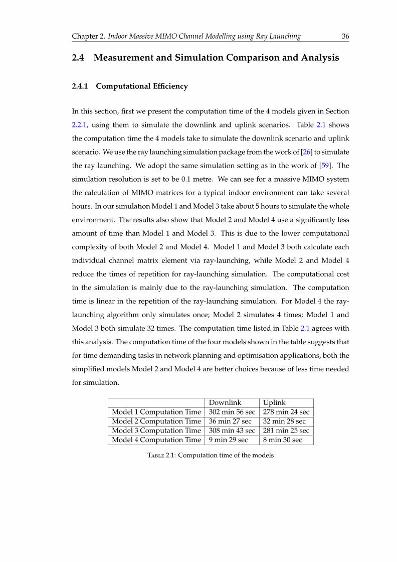
Chapter 2. Indoor Massive MIMO Channel Modelling using Ray Launching 36
2.4 Measurement and Simulation Comparison and Analysis
2.4.1 Computational Efficiency
In this section, first we present the computation time of the 4 models given in Section
2.2.1, using them to simulate the downlink and uplink scenarios. Table 2.1 shows
the computation time the 4 models take to simulate the downlink scenario and uplink
scenario. We use the ray launching simulation package from the work of [26] to simulate
the ray launching. We adopt the same simulation setting as in the work of [59]. The
simulation resolution is set to be 0.1 metre. We can see for a massive MIMO system
the calculation of MIMO matrices for a typical indoor environment can take several
hours. In our simulation Model 1 and Model 3 take about 5 hours to simulate the whole
environment. The results also show that Model 2 and Model 4 use a significantly less
amount of time than Model 1 and Model 3. This is due to the lower computational
complexity of both Model 2 and Model 4. Model 1 and Model 3 both calculate each
individual channel matrix element via ray-launching, while Model 2 and Model 4
reduce the times of repetition for ray-launching simulation. The computational cost
in the simulation is mainly due to the ray-launching simulation. The computation
time is linear in the repetition of the ray-launching simulation. For Model 4 the ray-
launching algorithm only simulates once; Model 2 simulates 4 times; Model 1 and
Model 3 both simulate 32 times. The computation time listed in Table 2.1 agrees with
this analysis. The computation time of the four models shown in the table suggests that
for time demanding tasks in network planning and optimisation applications, both the
simplified models Model 2 and Model 4 are better choices because of less time needed
for simulation.
Downlink UplinkModel 1 Computation Time 302 min 56 sec 278 min 24 secModel 2 Computation Time 36 min 27 sec 32 min 28 secModel 3 Computation Time 308 min 43 sec 281 min 25 secModel 4 Computation Time 9 min 29 sec 8 min 30 sec
Table 2.1: Computation time of the models

Chapter 2. Indoor Massive MIMO Channel Modelling using Ray Launching 37
1 2 3 4 5 6 7 8 9
Measurement Locations
-120
-100
-80
-60
-40
-20
0
Rec
eive
d P
ower
in d
Bm
MeasurementDeterministic ModelSimplified Deterministic ModelStatistical ModelSimplified Statistical Model
Figure 2.10: Average Received Power in Downlink
2.4.2 Received signal power
The received signal power is one of the most important parameters in network deploy-
ment and optimisation. It is closely related to the performance of the wireless networks.
According to (2.3) the received power at a certain location is calculated as
Ppx, y, zq “ qÿ
α“1
Aαpx, y, zqe´ jωταpx,y,zq2
Figure 2.10 shows the comparison between the average received power of the measure-
ments and the simulation results in the downlink scenario. Figure 2.11 shows the same
comparison result in the uplink scenario. We can see both results show good agreement.
The error between the simulation and measurements is calculated by the Root Mean
Square (RMS) error as:
E “1rt
m“r,n“tÿ
m“1,n“1
b
H2m,n ´ H2
m,n
where Hm,n is the simulated channel matrix.

Chapter 2. Indoor Massive MIMO Channel Modelling using Ray Launching 38
1 2 3 4 5 6 7 8
Measurement Locations
-90
-80
-70
-60
-50
-40
-30
-20
-10
0
Rec
eive
d P
ower
in d
Bm
MeasurementDeterministic ModelSimplified Deterministic ModelStatistical ModelSimplified Statistical Model
Figure 2.11: Average Received Power in Uplink
Following the above equation, we use the simulated channel Hm,n and the measured
channel Hm,n to calculate the RMS errors of the simulation models. The RMS error
results are presented in Table 2.2 and Table 2.3.
The results show that the RMS errors of Model 1 and Model 3 are smaller. The RMS
errors of Model 2 and Model 4 are higher but still mostly under 6 dB. This shows the
accuracy of Model 1 and Model 3 is higher than that of Model 2 and Model 4. This is
Location 1 2 3 4 5 6 7 8 9Model 1 RMS Error 3.2301 3.0285 3.4619 2.7061 3.1657 5.3280 2.3195 4.7964 3.3340Model 2 RMS Error 3.7594 5.4562 5.4561 5.0356 5.8612 5.7495 5.8634 5.6547 5.5598Model 3 RMS Error 4.7565 4.9863 4.8322 4.9879 4.1897 5.7882 4.6671 4.9882 4.3375Model 4 RMS Error 5.9781 5.3245 5.4215 5.7145 5.8771 5.8873 5.3227 5.9551 5.7723
Table 2.2: RMS Error in Downlink Scenario
Location 1 2 3 4 5 6 7 8Model 1 RMS Error 2.9568 2.2584 3.6514 3.9184 2.3808 2.3101 2.8085 2.2751Model 2 RMS Error 5.8631 5.7761 4.3343 5.4475 5.2403 5.9712 5.3315 5.9882Model 3 RMS Error 4.7701 4.2321 4.5642 5.4241 4.0214 4.0859 4.8794 4.9583Model 4 RMS Error 5.4578 5.3762 5.4772 5.6549 5.6873 5.0857 5.7544 5.7563
Table 2.3: RMS Error in Uplink Scenario

Chapter 2. Indoor Massive MIMO Channel Modelling using Ray Launching 39
Figure 2.12: Distribution of Received Power of Channel Elements in Downlink
because both Model 2 and Model 4 simplify the computation by using a single ray to
represent the whole array. The two simplified models trade certain degree of accuracy
for computational efficiency. However, the result shows that the overall accuracy of the
ray-launching models for massive MIMO systems is satisfying for the network planning
and optimisation purpose.
2.4.3 Distribution of Channel Elements
Massive MIMO channels are in a form of large channel matrix. The primary modelling
target for massive MIMO is to model the large channel matrices. We have 4 models
to generate the channel matrices according to (2.4). In this section, we choose the
measurement location 5 in the downlink scenario and measurement location 6 in the
uplink scenario to show the empirical distribution of the simulated channel elements.
In Figure 2.12 we present the cumulative distribution function (CDF) of the simulated
channel matrix elements of the downlink scenario in comparison with the measure-
ment. Model 2 is not included in this simulation as the power distribution of Model
2 is determined by the choices of the rays. We can see the simulated channel matrix
elements have a very close distribution to the measured channel matrix elements. This
demonstrates a good agreement between the simulation model and the measurement.
The uplink scenario result in Figure 2.13 shows a similar pattern as in the downlink
scenario. The above results demonstrate that the simulation models generate channel
matrix elements in good agreement with the measurement.

Chapter 2. Indoor Massive MIMO Channel Modelling using Ray Launching 40
Figure 2.13: Distribution of Received Power of Channel Elements in Uplink
1 2 3 4 5 6 7 8 9
Measurement Locations
0
5
10
15
20
25
30
35
40
45
50
Cha
nnel
Cap
acity
in B
its/S
econ
de/H
z
MeasurementDeterministic ModelSimplified Deterministic ModelStatistical ModelSimplified Statistical Model
Figure 2.14: Channel Capacity in Downlink
2.4.4 Channel Capacity Results
Channel capacity gain is one of the most attractive features of the massive MIMO
channel promised to the future wireless networks. In this part of the result, we present
the channel capacity comparison between the simulated channels and the measurement.
The MIMO channel capacity is calculated according to the equation:
C “ log detˆ
I`1
N0HH˚
˙

Chapter 2. Indoor Massive MIMO Channel Modelling using Ray Launching 41
1 2 3 4 5 6 7 8
Measurement Locations
0
5
10
15
20
25
30
35
40
45
50
Cha
nnel
Cap
acity
in B
its/S
econ
d/H
z
MeasurementDeterministic ModelSimplified Deterministic ModelStatistical ModelSimplified Statistical Model
Figure 2.15: Channel Capacity in Uplink
We apply the above MIMO channel capacity formula to calculate the MIMO channel
capacity from both the simulated channel matrices and the measured channel matrices.
Figure 2.14 shows the capacity result comparison in the downlink scenario. Figure 2.15
shows the capacity result comparison in the uplink scenario. Both figures show a good
agreement in the channel capacity between the simulated results and the measurement.
This demonstrates that the simulation models are accurate in estimating the channel
capacity. Therefore, the simulation models provide a reliable way to predict the channel
capacity in network planning and optimisation.
2.5 Conclusion
In this work, we propose to use ray launching model in massive MIMO channel mod-
elling in indoor environments. In order to limit the computational complexity in mas-
sive MIMO channels in network optimisation, we developed 4 ray-launching based
simulation models for modelling massive MIMO channel. The primary application
of these models is network planning and optimisation. We compare these simulation
models with the measurement in two real small cell network deployment environ-
ments. The comparison results show that the models have good agreements with the
measurement. Therefore, these 4 ray-launching based simulation models are efficient

Chapter 2. Indoor Massive MIMO Channel Modelling using Ray Launching 42
and accurate models, for planning and optimising networks equipped with massive
MIMO arrays.
The main contribution of this chapter is the 4 simplified modelling methods to tackle the
high computational complexity challenge in massive MIMO channels. These methods
reduced the complexity by exploiting the physical characteristics of the channel and
the propagation environments. Therefore, our results suggested that by incorporating
the physical characteristics of propagation channels, complexity and redundancy in the
computational models for massive MIMO can be avoided.

Chapter 3
Ray Launching based mmWave
Channel Modelling for Indoor
Propagation
3.1 Introduction
Wireless network planning and optimisation is a key component in network deploy-
ment. To meet the demand of optimal network services with minimal resource and
cost, network planning plays a key role in the deployment of the networks. Channel
map is one of the key tools that are essential in the planning and optimisation of the
networks geographically. The channel map is to indicate the channel characteristics
over the geographic map of the network deployment space. A channel map is used as
an essential tool to describe the channel condition geographically and then facilitates
the network deployment in the design space.
Channel maps are widely constructed through computer simulation based electro-
magnetic propagation predication tools. One of the popular models to simulate the
electromagnetic propagation is based on ray tracing. The early work in [9] first intro-
duced the simulation based channel predication software tools WiSE. It is based on the
electromagnetic propagation principles of geometrical optics (GO) and Uniform The-
ory of Diffraction (UTD). The software CINDOOR [10] is based on the same physical
propagation simulation and is specifically designed for indoor environment. The work
43

Chapter 3. mmWave Channel Modelling 44
in [69] extended the work to include diffusive diffraction in ray tracing. The recent
work in [70] also applied the ray tracing simulation to construct MIMO channels.
Another method is based on the numerical solution of the wave propagation equation
and Maxwell’s equations. The finite-difference time domain (FDTD) method gives a
numerical solution to the electromagnetic field in the time domain. Following the FDTD
algorithm, the work in [12] proposed a finite element based numerical method to build
a channel map efficiently.
The millimetre wave (mmWave) channel is proposed as a promising technique for the
future wireless networks. The channel has many unique characteristics. To deploy
networks equipped with mmWave channels, a channel map construction tool that is
capable of building mmWave channel map is essential. However, such a tool is still
missing. In this chapter, we propose a simulation based channel map construction tool
based on an intelligent ray launching algorithm (IRLA) [26], especially for modelling the
path loss value of 60 GHz indoor channel. It exploits the characteristics of the mmWave
channels to simplify the computational complexity of the traditional simulation tools,
while still preserves high degree of accuracy of the original physical electromagnetic
propagation models. The simulation model is then verified by the measurement result
in a real propagation environment.
The rest of the chapter is organised as follows. Section 3.2 describes the new ray tracing
based model. Section 3.4 is the comparison and analysis of simulation. Section 3.5 is
the conclusion.
3.2 The Path Loss Model based on Ray Launching
A widely used path loss model is the empirical model of log distance model. The model
is simply given as
PLpdq “ PLpd0q ` 10γ log10pdd0q (3.1)
where PLpdq is the path loss value at the distance d; PLpd0q is the path loss value at the
reference distance d0; γ is the path loss exponent. The path between the transmitter
and receiver can be seen as the sole propagation path chosen in the model. Hence, the

Chapter 3. mmWave Channel Modelling 45
model can be seen as a single propagation path model. It is an empirical model widely
used in modelling the path loss of propagation channel [71].
Wireless channel is widely modelled as multipath propagation. In multipath propaga-
tion model, the channel is written as
Hpdq “nÿ
i“1
ai expp´ jθipdiqq (3.2)
where Hpdq is the channel impulse response at distance d; i is the multipath index; n
is the number of the multipath components;di is the propagation distance of the i-th
multipath component; ai and θi are the amplitude and phase of the i-th multipath
component, respectively. For calculating the path loss value of the channel from the
multipath propagation model, we have the path loss value at d as
PLpdqmp “ ´ log10 |Hpdq|2 (3.3)
In traditional ray tracing algorithms, the path loss value is calculated according to (3.3).
The value of the total channel effect Hpdq in multipath propagation is characterised
through tracing the individual propagation paths. It is realised in GO and UTD [60].
However, the simulation of GO and UTD is computationally heavy. For the purpose of
calculating the path loss value, we can adopt the simple log distance model in (3.1).
In our model, we calculate the path loss value of each individual multipath component
via the ray launching simulation. Thus the path loss value becomes:
PLpdqmpe “1n
nÿ
1
plpdiq (3.4)
where PLpdqmpe is the path loss value at distance d; PLpdiq is the path loss value of the
i-th multipath component. In appearance, the model in (3.4) differs from the model
in (3.3). However, next we will show that the model in (3.4) is adequately accurate in
comparison to the model in (3.3).
With a fixed distance d, we write the path loss value in (3.4) as
PLmpe “´řn
i“1 10 log10 |ai|2
n(3.5)

Chapter 3. mmWave Channel Modelling 46
0 20 40 60 80 100
Individual Path Loss Value Range in dB
0
0.1
0.2
0.3
0.4
0.5
0.6
0.7
0.8
0.9
1
Diff
eren
ce B
etw
een
Tw
o P
ath
Loss
Mod
els
D in
dB 20 Paths
10 Paths5 Paths
Figure 3.1: Path Loss Calculation Difference Using Sum-and-Average
and the path loss value from multipath propagation (3.3) as
PLmp “ ´10 log10 |
nÿ
i“1
ai expp´ jθiq|2 (3.6)
We define the difference between the two path loss values as D in the equation below,
and it has the unit in dB.
D “ |PLmpe ´ PLmp| (3.7)
In Figure 3.1, the value D is plotted against the loss value of the individual paths. The
difference between the two models becomes negligible in the high path loss region.
When the path loss values fall in the region above 20 dB, the difference is negligible.
In this region, the path loss value calculated by (3.4) is a good approximation of the
original multipath model.
This result shows that the model in (3.4) is adequately accurate in modelling the path
loss values for channels in the path loss value region above 20 dB. To consider the
realistic application of the model in network planning, the poor coverage where the
path loss is high, is more to the interests of the network planning. Therefore the model
offers a reasonable approximation to the original multipath propagation model. We can
draw the following observation:

Chapter 3. mmWave Channel Modelling 47
Proposition 3.1. When the path loss values are in the region of larger than 20dB, the model in
(3.4) is a good approximation to the model in (3.3).
The model in (3.4) calculates the path loss value of each individual multipath and
average the values. The advantage is that the calculation avoids the complexity of
modelling the environment for the GO and UTD and still considering the multipath
propagation mechanism of the wireless channel. By focusing on the path loss values,
the computation can be significantly simplified without considering the GO and UTD.
The drawback is that it is only suitable as an approximate model for the path loss values.
In the 60 GHz frequency band, the advantage of the model is even more obvious. The
high path loss exponent of the 60 GHz frequency makes the high path loss region
significantly smaller. In path loss channel map construction, the model has higher
accuracy in even the vicinity regions of the network planning region.
The value of D against the distance is plotted in Figure 3.2. The figure shows that over
the propagation distance of 0.1 metre, the difference between the two models is below
0.025 dB. With the increase of the propagation distance, the difference drops quickly.
When the propagation distance is over 0.5 metre, the difference is negligible. This result
shows that the 60 GHz frequency band has significantly reduced the suitable distance
of adopting the model in (3.4).
For 60 GHz band indoor channels, we simplify the model in (3.4) by omitting the diffrac-
tion in the propagation. Thus the empirical path loss in the propagation calculation
only considers the reflection and transmission in the propagation. The comparison be-
tween the simulation results and measurement in Section 3.5 shows this is an acceptable
approximation in indoor path loss prediction.
The path loss of the reflected path is given as:
PLr f “ PLpdq ´ 10 log10 |Γ2| (3.8)
where PLpdq is the empirical path loss values through the distance d; Γ is the Fresnel
reflection coefficient.

Chapter 3. mmWave Channel Modelling 48
0.1 0.2 0.3 0.4 0.5 0.6 0.7 0.8 0.9 1
Propagation Distance in Metre
0
0.005
0.01
0.015
0.02
0.025
0.03
The
diff
eren
ce b
etw
een
the
two
mod
els
D in
dB
Figure 3.2: The Value of D vs the Propagation Distance
And the path loss value for transmission is given as:
PLtr “ PLpdq ´ 10 log10 |1´ Γ2| (3.9)
We use the three single loss values in (3.1), (3.8) and (3.9) to calculate the path loss value
in each multipath component. Thus the total path loss of an individual path is written
as:
PLi “ PLpdq ` PLr f ` PLtr (3.10)
The path loss exponent value in (3.10) is chosen as γ “ 2.2 for an indoor office en-
vironment with 60 GHz according to [71]. To trace the multipath propagation in the
environment, we adopt an intelligent ray launching algorithm (IRLA) from [26]. The re-
flection coefficient values for various materials at 60 GHz in indoor office environments
are taken from the work in [72]. The individual path loss values from the multipath
components are then used to obtain the total path loss values. Following the model in
(3.4), the path loss value now can be written as:
PLsa “1n
nÿ
i
PLi (3.11)

Chapter 3. mmWave Channel Modelling 49
Figure 3.3: Buidling Floor Map
where PLi is given in (3.10) and n is the total number of the chosen paths.
3.3 Channel Measurement
In this section, we briefly describe the channel measurement settings. The measure-
ment environment is a typical office environment in the Department of Engineering at
Durham University. The floor map is shown as in Figure 3.3. The floor is carpeted.
The doors are wooden. The windows contain metal frames. The walls are bricks with
plastered outer layer. There are some inner walls and doors are replaced by glass. The
ceiling is made of plastic material. An overview of the measurement environment is
shown in Figure 3.3.
The channel information is measured using the Durham channel sounder. The transmit-
ter antennas and the receiver antennas are horn antennas. More detailed information
about the channel sounder can be found in the work of [68]. Both the transmitter and
the receiver are equipped with 2 antennas. The height of the transmitter is 2.35 metre.
The height of the receiver is 1.46 metre. The centre frequency of the measurement is

Chapter 3. mmWave Channel Modelling 50
Figure 3.4: 3D Buidling Model
60 GHz. The measurement campaign was carried out in the Department of Computer
Science of Durham University in the spring of 2014.
After the channel sounder was calibrated, the measurement was carried in the environ-
ment with the transmitter fixed. The location of the transmitter is indicated in Figure
3.3 as point ’A’. The height of the transmitter is fixed at the ceiling to emulate the typical
placement of an indoor wireless network access point. Various receiver locations are
chosen. The receiver locations are drawn along the red line in Figure 3.3 with various
distances specified. The channel sounder data are recorded and processed. The path
loss value at each measurement location is averaged over the 2 transmitter antennas
and 2 receiver antennas. Thus, each measurement location has only one averaged path
loss value.
3.4 Simulation Results and Comparison
The simulation is carried out using the path loss model in (3.4) based on the (IRLA)
algorithm in[26]. The environment is modelled in a 3D building structure. The indoor
environment is included in the model. The walls, doors, and windows are all included
in the 3D building model. The 3D building model is shown in Figure 3.4. The simulation
result of the path loss is shown in Figure 3.5. A 2D view of the path loss map is shown
in Figure 3.6.
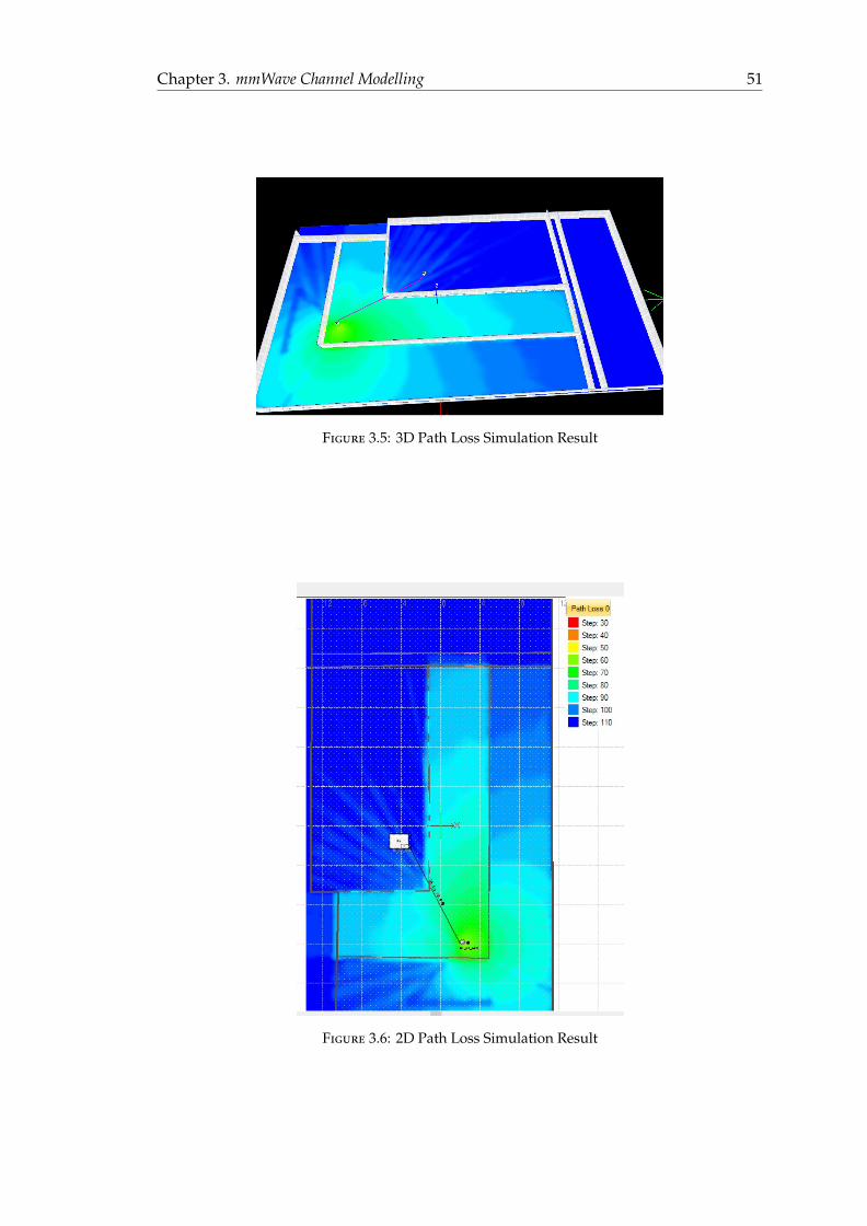
Chapter 3. mmWave Channel Modelling 51
Figure 3.5: 3D Path Loss Simulation Result
Figure 3.6: 2D Path Loss Simulation Result

Chapter 3. mmWave Channel Modelling 52
Figure 3.7: Path Loss Value Comparison
The comparison between the simulation and the measurement result is shown in Figure
3.7. The measurement locations are chosen along the red straight line in the map. In
total 50 measurement locations are chosen. The simulation is set to 0.2m resolution.
In Figure 3.7, the red curve is the simulation results. The blue curve is the measurement
result. The simulation result gives a good overall prediction of the path loss in the
scenario. In most measurement locations, the error is below 3 dB. The overall Root
Mean Square (RMS) error is 2.5028 dB. This demonstrates the simulation gives a good
prediction to the path loss values in the environment.
3.5 Conclusion
In this chapter, first we analysed the modelling difference between the traditional mul-
tipath propagation model in (3.3) and an averaged path loss value model in (3.4). My
analytical result showed that when the path loss values are high, the difference between
the models is negligible. Based on this observation, I propose a path loss model for the
60 GHz indoor channel using the model in (3.4). The path loss model is an implemen-
tation of multipath empirical path loss model based on ray launching algorithm. The
simulation model result is also compared with the measurement data in a typical in-
door office scenario. Comparison between the simulation results and the measurement

Chapter 3. mmWave Channel Modelling 53
demonstrates that the proposed model is an accurate model for indoor channel path
loss prediction in the 60 GHz band.
The main contribution of this chapter is a new path loss model based on ray launching
for mmWave frequency channel. By exploiting the characteristic of high attenuation of
the mmWave channel, an efficient computational ray based path loss model is developed
in this chapter. The results of this channel model suggest that channel models for the
mmWave frequency can benefit from exploiting the unique characteristics of the channel
at this frequency range.
Chapter 4
A Vector MIMO Channel Map
Construction and Its Applications
4.1 Introduction
With the increasing demand for higher data rate communication, wireless network
operators are facing the challenge of providing high quality network service. Network
planning planning plays a central role in meeting the ever increasing demand for high
data rate wireless communication. The purpose of network planning is to deploy the
network nodes in optimal locations to provide guaranteed quality of network service.
In conventional network planning, coverage planning is the key stage in the planning
process. The aim of the coverage planning is to achieve optimal radio signal coverage
by selecting the optimal base station locations for the network.
Many research works have focused on finding the optimal base station locations to
achieve the optimal network performance. Early works in the network planning fo-
cused on achieving the coverage planning goal. The early work of [2] gave a non-linear
optimisation model for the problem of finding the optimal transmitter location in micro-
cellular networks. The work of [3] investigated the optimisation algorithms for the base
station location placement in Universal Mobile Telecommunications System (UMTS)
networks, with the consideration of not only signal overage but both of network traffic
and power control. Following this research, the work of [4] made the effort to optimise
the UMTS network coverage by optimising the antenna configuration, which can be
54

Chapter 4. A Vector MIMO Channel Map Construction and Its Applications 55
seen as a step further ahead from base station location optimisation. A recent work
of [5] studied the optimisation algorithms for base station placement and proposed a
hierarchical search algorithm for the optimisation problem. The network base station
location optimisation problem has been an active research topic since the second gen-
eration wireless network and it is still a key problem for the next generation networks,
such as heterogeneous networks (HetNet)[6].
To achieve the target of optimal base station deployment, a signal coverage map over
the deployment space is essential. Various candidate locations in the map are compared
and the optimal one is chosen. Such a coverage map is widely used in the network
planning practice. Many researches have been devoted for such a coverage map for
network planning purposes. The pioneering work in [7] partitioned the map into areas
and adopted an empirical model to predict the path loss contour plot as a path loss
map. The work in [8] followed this method and extended it to an outdoor-indoor
transient situation. To accurately predict the channel information requires significant
amount of computation, therefore many research works are devoted to computer-based
simulation. Early works such as the WiSE tools by Bell Labs [9] and CINDOOR [10]
were specially designed for designing and planning indoor networks. The method of
building such channel maps is mainly the deterministic channel propagation model,
which contains roughly two major modelling methods: FDTD related models and ray
based models. The work of [11] first used the name of channel map and proposed
a ray tracing method for building the channel map. The work in [12] proposed an
efficient computational electromagnetics method for building the channel map. For a
complete review of channel modelling in HetNet, I refer the readers to the work of [6].
The channel map has long been widely used as an essential tool in network design.
However, it still lacks a rigorous mathematical formulation, which limits the further
development of the channel map as an essential tool in network planning, especially
for MIMO network planning.
With the application of the modern advanced wireless transmission techniques, such
as MIMO system, the network performance is largely benefited from those advanced
techniques. These advanced techniques are widely deployed in the current and fu-
ture generation wireless networks, such as HetNet [6]. Meanwhile, to plan networks
equipped with these advanced techniques, network planning tools face the challenges
of considering these advanced techniques in the planning process. Many challenges

Chapter 4. A Vector MIMO Channel Map Construction and Its Applications 56
stem from a lack of high dimensional vector form for the channel map. Although the
channel map has been widely used as a tool in network planning, a vector form for the
channel map has been missing. This limits the development and functionality of the
channel map as a tool in advanced network planning, such as MIMO network plan-
ning. The major challenge that facing the conventional channel map tools in MIMO
channel modelling is the limitation the 2 dimensional channel map. A conventional 2
dimensional channel map lacks the capability to accommodate the higher dimensions
of the MIMO channel. The intrinsic drawback of representing the channel distribution
in a 2 dimensional or 3 dimensional map failed to capture the MIMO channel in higher
dimensions. Because of the higher dimensions of the vector form of the MIMO system,
in order to apply the conventional 2 dimensional channel map for MIMO systems, we
need to extend the channel map to a vector form.
The purpose of the chapter is to present a straightforward vector form the channel map
to the MIMO system based on a mathematical formulation to the vector form of the
channel map. Although in practice, the extension to vector form appears straightfor-
ward, this is not true in higher dimension MIMO channel, especially in distributed
MIMO channel. In such MIMO channels, conventional single transmitter channel map
struggles to provide a complete picture of the channel by using 2 dimensional or 3
dimensional maps. To overcome this challenge, we give a vector channel map in a
mathematical form. We then also show that this vector form channel map can be con-
structed based on the conventional 2 dimensional channel map. We further apply this
vector channel map to a distributed MIMO network planning and optimisation sce-
nario, which demonstrates the vector channel map as an effective and straightforward
extension of a conventional 2 dimensional channel map.
The rest of the chapter is as follows: Section 4.2 gives the definition of channel map for
both SISO and MIMO channel. Section 4.3 presents a method of building channel maps
for distributed MIMO networks. Section 4.4 gives a numerical example to illustrate
the construction of a channel map for distributed MIMO network in a typical network
planning scenario. Section 4.5 concludes the work.

Chapter 4. A Vector MIMO Channel Map Construction and Its Applications 57
4.2 Mathematical Formulation of Channel Map
4.2.1 Single Antenna Channel Map
Channel map has been widely used in network planning. In a deterministic propa-
gation setting, when the transmitter location and propagation configuration is fixed,
the channel is then determined from a deterministic channel modelling perspective.
In such a scenario, a channel map can be drawn to present the channel information
over the signal coverage space. A channel map is designed to give an overview of the
channel information over the design space in the form of a map.
In conventional channel maps, the most commonly interested channel parameter is the
power information. This is due to the conventional network planning targets, for which
coverage planning is the primary target. The coverage planning relies on the power
parameters, such as path loss and signal to noise ratio, of the channel information.
However, for modern network planning other parameters such as phase and delay are
also of interest. Our channel map definition incorporates complete channel information.
In channel map, the receiver location information in the map is modelled as a discrete
locational set. In most cases, it is modelled as a discrete grid over the design space. Each
potential receiver location is specified by its Cartesian coordinate location. Therefore
the receiver locations in the grid covering the map is given as a set:
L “ tpx, y, zq P R3|px, y, zq are the Cartesian coordinates of locations in the mapu (4.1)
The set is a finite set. In channel map, it is common to plot the channel information
over all the potential receiver locations, with a fixed source location. Then the receiver
location set is given as the location set L subtracting the source location s. It is denoted
as:
M “ Lztsu (4.2)
The number of the potential receiver locations is the cardinality of the set and is denoted
as |M|.
Under the assumption that the channel is a narrow band static channel, the channel
information set is given as the set of complex number C.

Chapter 4. A Vector MIMO Channel Map Construction and Its Applications 58
The channel map is defined as a function mapping from the location setL to the channel
setC. The wireless channel can be modelled as the electromagnetic field in the coverage
space. In electromagnetic channel modelling, the channel value at a location is the
electric field value of the electromagnetic field [73, 74]. Thus we can write:
Hps, lq “ Eps, lq (4.3)
where Eps, lq is the electric field at location l and with the source radiating at location s,
and Hps, lq represents the channel information at location l, with the radiating source at
location s.
Following the above definitions, we can give a definition of the single antenna channel
map
Definition 4.1. (Single Antenna Channel Map) A single antenna channel map is defined
as the set of channel map functions that gives the mapping from the physical location
setM to the channel information set C.
Thus, we can write the channel map as a function:
f :MÑ C where f plq “ Hps, lq (4.4)
This definition gives a mathematical formulation of the widely used single antenna
channel map in network planning. The channel map is a function that maps the
potential receiver locations in a physical map to the channel information. The channel
map describes the channel information over the location map.
The channel map function characterises the channel information over the design space.
The channel map function at each potential location is determined by the physics of
the propagation. Therefore each map function can be written in the form of a Green
function [75] as:
Hps, lq “ż
s
Gpp, lqJppqdp (4.5)
where Gpp, lq represents the Green function with source at p and the field value at l; Jppq
denotes the source current at p; p is the points in the source domain s; the integral is over

Chapter 4. A Vector MIMO Channel Map Construction and Its Applications 59
the source current. In practice there are specific numerical electromagnetic simulation
tools to solve the channel map, such as in [12, 49].
4.2.2 MIMO channel map
For MIMO channel map, the multiple transmitters of the MIMO channel are assumed
to be determined at fixed locations. The objective of the MIMO channel map as in the
single antenna channel map is to draw a channel information map over the potential
receiver locations.
Based on the formulation of the single antenna channel map, we have a vector form
of channel map for MIMO systems. In MIMO the propagation channel is extended to
multiple transmitters. The channel information is to track each sub-channel between
each transmitter and receiver pair. In this case, we write the channel map of multiple
transmitters in a form of channel map vector. Each element in the channel map vector
is a single antenna channel map generated by one single transmitter. Thus we define
the channel map vector as:
Definition 4.2. (Channel Map Vector) A channel map vector is defined as a vector of
the channel maps with the same location setM. It is written as:
p f1pMq, f2pMq, .... fnpMqq (4.6)
where fi is the i-th channel map.
For the MIMO system, the potential multiple receiver locations form a set of receiver
location vector
Lv “ tpl1, l2, .....lmq|li PMi for all 1 ď i ď mu. (4.7)
whereMi is the potential receiver location set for the i-th map. Each element in the set
Lv is a receiver location vector, identifying the multiple receiver locations. By applying
the receiver location vectors to the channel map vector in (4.2), we obtain the MIMO
channel matrices.

Chapter 4. A Vector MIMO Channel Map Construction and Its Applications 60
The channel information for MIMO systems is a complex matrix and the set of channel
information can be written as Cmˆn. The channel map function is also written in a
matrix form. Each element in the matrix form corresponds to a transmitter-receiver
pair in the channel matrix.
HpS,Lq “
»
—
—
—
—
—
—
–
H1,1ps1, l1q H1,2ps2, l1q ¨ ¨ ¨ H1,mpsm, l1q
H2,1ps1, l2q H2,2ps2, l2q ¨ ¨ ¨ H2,mpsm, l2q...
.... . .
...
Hn,1ps1, lnq Ht,2ps2, lnq ¨ ¨ ¨ Hn,mpsm, lnq
fi
ffi
ffi
ffi
ffi
ffi
ffi
fl
(4.8)
Like in the single antenna channel map, the channel information can also be represented
by the electric field values in a matrix form:
HpLq “ EpLq (4.9)
Similar as in the single antenna channel map definition, we define the MIMO channel
map as the mapping functions from the receiver location vector set to the channel matrix
set. The definition is given as follows.
Definition 4.3. (Vector Channel Map) The MIMO channel map is defined as the set of
functions that maps the receiver location vector setLv to the channel matrix set HpS,Lq
as:
F : Lv Ñ Cmˆn where FpLq “ HpS,Lq (4.10)
According to the representation of the electrical field value, the electrical field value
EpLq can also be written in a matrix form:
EpLq “ż
»
—
—
—
—
—
—
–
G1,1pl1q G1,2pl1q ¨ ¨ ¨ G1,mpl1q
G2,1pl2q G2,2pl2q ¨ ¨ ¨ G2,mpl2q...
.... . .
...
Gn,1plnq Gt,2plnq ¨ ¨ ¨ Gn,mplnq
fi
ffi
ffi
ffi
ffi
ffi
ffi
fl
»
—
—
—
—
—
—
–
J1pSq
J2pSq...
JnpSq
fi
ffi
ffi
ffi
ffi
ffi
ffi
fl
dp (4.11)
This definition gives a mathematical formulation of the MIMO channel map. Compar-
ing to the single antenna channel map, the MIMO channel map function is a vector

Chapter 4. A Vector MIMO Channel Map Construction and Its Applications 61
Figure 4.1: An Illustration of Distributed Antennas MIMO System
function. It maps the potential receiver location vectors to the channel information ma-
trix. It gives the channel information over the potential receiver locations in the form
of a map. The locations in the map are vectors. Such a mathematical formulation has
the advantage of representing the abstract location vectors in a vector form map. This
feature overcomes the limitation of representing channel information over the 2D or 3D
physical map but offering an abstract channel map representing channel information
over abstract location vectors. We will utilise this feature in an example of planning
distributed MIMO systems in Section 4.4.
4.3 Construction of MIMO channel map using distributed an-
tenna systems
The MIMO has been investigated as one of the key techniques for achieving the high
capacity network since the seminal works of [76, 77]. Recently, researchers have focused
on applying MIMO techniques in HetNet, especially the distributed MIMO integrated
with HetNet [78]. A distributed MIMO system is illustrated in Figure 4.1. In a dis-
tributed MIMO system, the multiple antennas in the MIMO systems are not mounted
on a conventional antenna array, while they are connected to a central controller to
form a distributed antenna array. In HetNet, such a distributed MIMO system can be
realised via the cooperation between different tiers of the networks.
We study the method to construct the MIMO channel map based on conventional
single antenna channel map in this section. We first introduce the single antenna
channel map building tool in network planning. Then we investigate the application

Chapter 4. A Vector MIMO Channel Map Construction and Its Applications 62
Figure 4.2: An Example of Single Antenna Channel Amplitude Map
of the channel map formulation to build MIMO channel map in practice. The focus
is to build channel map for networks using distributed MIMO systems. The method
follows the formulation of the channel map in the previous section. This demonstrates
the application of the channel map formulation in construction of channel maps.
Computational electromagnetic tools are widely used to simulate the propagation of
radio waves and predict the channel information in network planning. In this section,
we focus on using a single antenna propagation simulation tool to build MIMO channel
maps. An example result of channel amplitude information map generated by the
simulation tool iBuildNet [79] is shown in Figure 4.2.
According to the definition of the channel map, the channel map predicted by the
simulation is a set of channel values mapping onto the location set. In this single
antenna channel map case, the locations are the physical locations in the map. Thus, the
channel map represents the channel information at each potential location in the map. In
distributed antenna systems, the antennas are deployed in a distributed way. Due to the
distance between the antennas, we assume the mutual coupling effect between antennas
is negligible. So we can simulate the multiple antenna channel map individually
without considering the mutual coupling widely existed in antenna array systems.
Under such an assumption, the conventional single antenna channel map construction

Chapter 4. A Vector MIMO Channel Map Construction and Its Applications 63
Figure 4.3: Channel Amplitude Map Vector
tools by simulating radio wave propagation are suitable in the distributed antenna
system case.
With multiple distributed transmitter antennas, the multiple single antenna channel
maps generated by single transmitter antenna are arranged to be a channel map vector.
Following the single antenna channel map example in Figure 4.2, we set 4 distributed
transmitter antennas and construct the channel map vector as in Figure 4.3. Each
element map in the vector is a channel map constructed according to one single antenna
channel map.
According to the definition of the MIMO channel map, the receiver location vector set is a
key component in the construction of the channel map. We discuss the receiver antennas
in two different scenarios: traditional antenna arrays and distributed antenna systems.
The traditional antenna array is even equipped in mobile terminals. On the other hand,
for distributed multiple receiver antennas, it normally requires cooperation between
the receiver antennas. It has potential in future wireless network applications, such as
high data rate wireless backhaul connections. In this work, we assume the distributed
antennas have perfect synchronisation and are deployed in a fully distributed way.
We first study the MIMO channel map construction for multiple receiver antenna using
antenna arrays. We assume that the resolution of the map is adequately high to resolve
the elements in the receiver array. In this case, the receiver antennas can be represented
by the location points in the channel map. Given the fixed array size, geometry and
orientation, the receiver location vector is specified using the locations in the map.

Chapter 4. A Vector MIMO Channel Map Construction and Its Applications 64
The location point set of the channel map in the multiple distributed transmitter antenna
channel map is the location set excluding the transmitter locations. It is given as:
M “ Lzts1, s2, . . . smu (4.12)
Following the MIMO channel map Definition 4.3, we have the receiver location vector
set as:
Lv “ tpl1, l2, . . . lmq|li PM for 1 ď i ď mu (4.13)
Each receiver location vector pl1, l2, . . . łmq corresponds to a potential location vector for
the array deployment. Each location point li in the vector is a physical location point in
the map. For each element channel map in the channel map vector, the location point
sets only differ in the transmitter location si.
Under the assumption of fixed array size, geometry and orientation, we can use a single
location point in the set to specify the location of the array. The locations of the rest of
the elements in the array can be determined through the geometry of the array. Such a
method has been used in modelling the MIMO channel using antenna arrays [80]. In
this way, the potential location vector set Lv for array location degrades to the set of the
single location point set of the mapM. The relationship can be written as :
p :MÑ Lv where pplq “ pl1, l2, . . . lmq (4.14)
This relationship summarises that the receiver location vector can be replaced by a
single location MIMO channel map using antenna array. As the receiver location vector
set degrades to the receiver location point set, the MIMO channel map can be built
following Definition 4.3 in (4.10). Such a form of MIMO channel map for network
planning purposes has been studied in the work of [34, 81]
On the other hand, in MIMO channel map using distributed receiver antenna systems,
the receiver locations are chosen from the individual maps in the channel map vector.
In this case, the target is to construct an m ˆ n distributed MIMO channel map. The
m receiver antenna locations are chosen from the locations in the map excluding the n

Chapter 4. A Vector MIMO Channel Map Construction and Its Applications 65
transmitter locations. The receiver location vector can be written as:
L “ pl1, l2, . . . lmq P tMˆMˆ . . .Mu (4.15)
where ’ˆ’ represents the Cartesian product of the set. This relation describes the
receiver locations for a distributed antenna system are chosen from the combinations
of the potential locations in the map.
By the above description for the potential receiver location set, the potential receiver
locations are all the possible combinations of m different locations in the map location
set. Therefore, we have the following proposition regarding the total number of the
potential locations in the channel map.
Proposition 4.4. The total number of potential locations in a m ˆ n MIMO channel map is
the combination of the m receiver locations from the location set in the map excluding the n
transmitters. It is given as
M “ Cm|M|´n (4.16)
Each element in the receiver location vector set corresponds to one potential location
combination for the multiple receiver antennas. The location vector L “ pl1, l2, . . . lmq
specifies the location of the m receiver antenna location in a vector form. Applying
this location vector in the single antenna channel map identifies a channel information
vector which corresponds to a single-input multiple-output (SIMO) channel vector,
which is one column vector as in (4.8). While applying this vector to a channel map
vector, the result is a channel matrix.
At this stage, the MIMO channel map construction is completed by looking up the
corresponding channel values at each location from the single antenna channel map.
This method preserves the conventional single antenna channel map and extends it to
build distributed MIMO channel maps.

Chapter 4. A Vector MIMO Channel Map Construction and Its Applications 66
The resulting matrix is written as:
HpLq “
»
—
—
—
—
—
—
–
f1pl1q f1pl2q ¨ ¨ ¨ f1plmq
f2pl1q f2pl2q ¨ ¨ ¨ fmplmq...
.... . .
...
fnpl1q fnpl2q ¨ ¨ ¨ fnplmq
fi
ffi
ffi
ffi
ffi
ffi
ffi
fl
(4.17)
The matrix elements fipl jq denotes the channel information in the i-th channel map at
location l j.
Each channel vector L in the receiver location vector map determines one channel matrix.
The channel matrix corresponds to the MIMO channel matrix with the distributed
receiver antennas located by the vector L. The channel matrix specifies the MIMO
channel matrix with multiple transmitter antennas given in the form of channel map
vector and the multiple receiver location vector which is used to identify the channel
matrix at each possible receiver location combination.
4.4 Numerical Examples
In this section, we give an example of the MIMO channel map to demonstrate its
application in distributed MIMO systems. Following the method in Section 4.3, we build
a distributed MIMO channel map for a typical indoor network deployment scenario.
The simulation tool for single channel map construction is the Par-Flow simulation
method presented in [12, 82, 83].
The simulation scenario is a typical office environment. The floor map is shown in
Figure 4.4. The environment comprises walls, doors, windows and ceilings as a typical
indoor network planning scenario. The frequency is set to be 2.4 GHz. The bandwidth
is set to be 15 KHz as one single carrier bandwidth in the long term evolution (LTE)
networks. We deploy a 2ˆ 2 distributed MIMO system in the environment.
The 2 transmitter antennas are deployed in a distributed way. For the reason of demon-
stration, we only choose one set of locations to deploy the 2 distributed transmitter
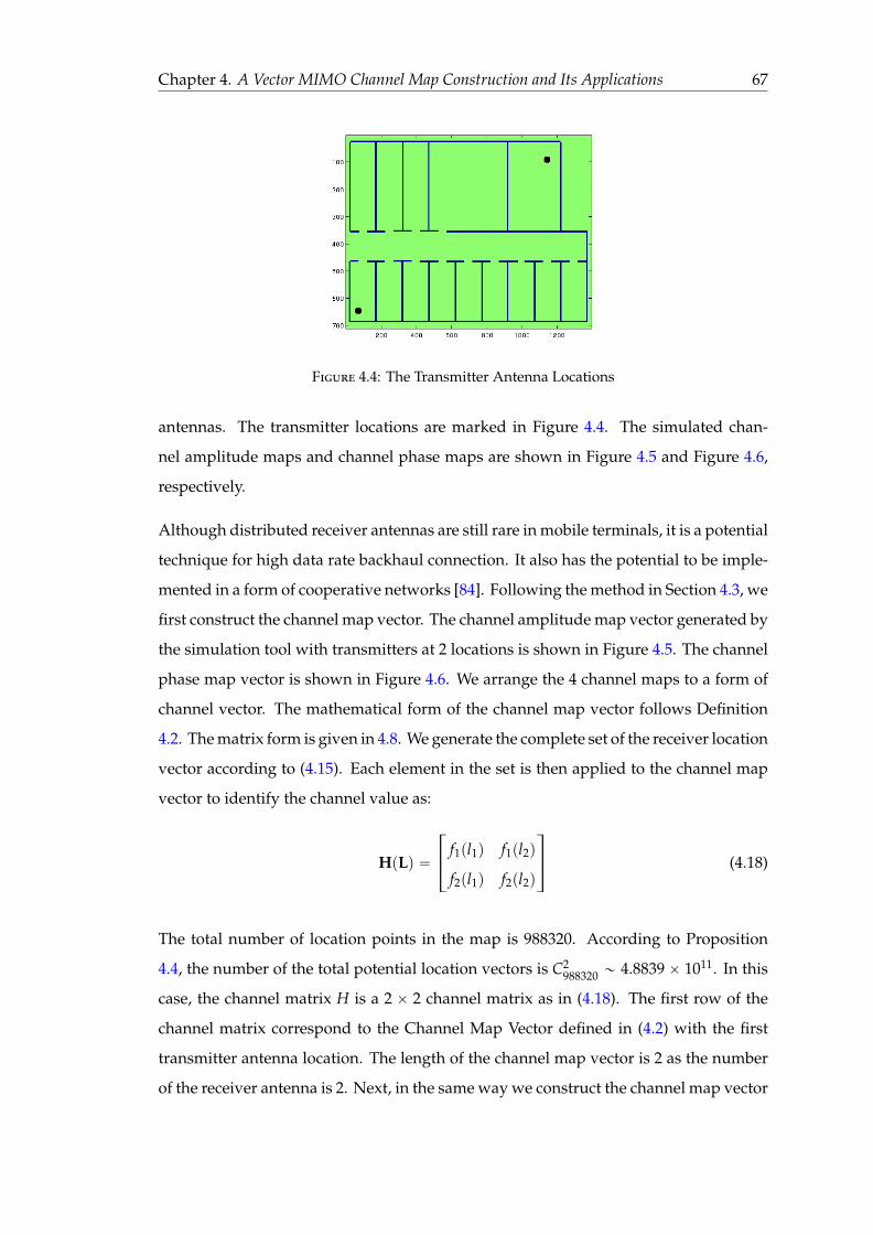
Chapter 4. A Vector MIMO Channel Map Construction and Its Applications 67
Figure 4.4: The Transmitter Antenna Locations
antennas. The transmitter locations are marked in Figure 4.4. The simulated chan-
nel amplitude maps and channel phase maps are shown in Figure 4.5 and Figure 4.6,
respectively.
Although distributed receiver antennas are still rare in mobile terminals, it is a potential
technique for high data rate backhaul connection. It also has the potential to be imple-
mented in a form of cooperative networks [84]. Following the method in Section 4.3, we
first construct the channel map vector. The channel amplitude map vector generated by
the simulation tool with transmitters at 2 locations is shown in Figure 4.5. The channel
phase map vector is shown in Figure 4.6. We arrange the 4 channel maps to a form of
channel vector. The mathematical form of the channel map vector follows Definition
4.2. The matrix form is given in 4.8. We generate the complete set of the receiver location
vector according to (4.15). Each element in the set is then applied to the channel map
vector to identify the channel value as:
HpLq “
»
–
f1pl1q f1pl2q
f2pl1q f2pl2q
fi
fl (4.18)
The total number of location points in the map is 988320. According to Proposition
4.4, the number of the total potential location vectors is C2988320 „ 4.8839ˆ 1011. In this
case, the channel matrix H is a 2 ˆ 2 channel matrix as in (4.18). The first row of the
channel matrix correspond to the Channel Map Vector defined in (4.2) with the first
transmitter antenna location. The length of the channel map vector is 2 as the number
of the receiver antenna is 2. Next, in the same way we construct the channel map vector

Chapter 4. A Vector MIMO Channel Map Construction and Its Applications 68
Figure 4.5: Channel Amplitude Map Vector
Figure 4.6: Channel Phase Map Vector
for the second transmitter location using the channel map of the second transmitter
location. After obtaining both channel map vectors, by aligning the 2-element vector
from the first set and the 2-element vector from the second set into a 2 matrix form, we
have the channel matrix for one potential location combination for receiver antenna.
In order to construct the full channel map set all the possible location combination for
receivers, we need to list all the possible 2 location combination in the map with the
number of C2988320 „ 4.8839ˆ 1011.
It costs high computational resource to search the whole possible combinations of the
receiver locations. We sample the 988320 receiver locations uniformly to choose 2000 lo-
cations as the candidate locations. Thus, the searching space reduces to C22000 “ 1999000.
It could be argued that the truly optimal locations are outside our searching space due
to the sampling. However, the purpose of this example is to show the effectiveness
of the vector channel map in network optimisation and also its simple construction
based on conventional channel map tools. When precision of the optimisation result is
required, we can still search over the whole possible candidate locations to achieve the
optimal performance.

Chapter 4. A Vector MIMO Channel Map Construction and Its Applications 69
Figure 4.7: The CDF of Capacity in Distributed MIMO
4.4.1 Channel Capacity Optimisation
In this part, we optimise the network performance by choosing the receiver locations
which achieves the maximum channel capacity.
We look up the channel matrix values in the channel map corresponding to all the
receiver location vectors. The result is a table mapping from the receiver location vector
to the corresponding channel matrix. Under the assumption of independent noise at
each receiver and with uniform power allocation at the transmitter, we then use the
channel matrix to calculate the MIMO channel capacity, according to the formula:
C “ log2 detpI ` snrHH˚q (4.19)
where H is the channel matrix and H˚ is the Hermitian transpose of the channel matrix;
detp¨q is the determinant of the matrix and snr is the signal to noise ratio at the receiver.
The transmitting power is set to be 20 dBm. The thermal noise power is given as
N “ kTF, where k is the Boltzmann’s constant; T is the temperature in kelvin and F is
the bandwidth [85]. Using this formula, as the bandwidth is assumed as 15 KHz and the
temperature is assumed as room temperature of 20 degree Celsius, the thermal noise
power is obtained as ´132 dBm. Plugging the transmitting power and the thermal
noise power with the channel matrices from the channel map construction, the channel
capacity values are calculated for all the channel matrices constructed in the channel
map set.

Chapter 4. A Vector MIMO Channel Map Construction and Its Applications 70
Figure 4.8: The PDF of Capacity in Distributed MIMO
Figure 4.9: The Optimal Locations for Receiver Antennas
The cumulative distribution function (CDF) of the resulting channel capacity is shown
in Figure 4.7. The probability density function (pdf) of the capacity is shown in Figure
4.8. The statistics of the resulting capacity values are summarised in Table 4.1. The
mean value of the capacity is 31.5006 bits/s/Hz and the maximum value is 86.4459
bits/s/Hz. The optimal receiver antenna locations that achieve the maximum capacity
are indicated in Figure 4.9.
Table 4.1: Statistics of the Capacity Values
Maximum Minimum Mean Median standard deviation86.4459 0.0144 31.5006 30.2073 11.5412
The gain of optimally designed receiver location from an arbitrarily random choice of
receiver locations is significant in this case. We can see that the majority of the receiver
locations support a capacity near the mean value of from 20 to 40 bits/s/Hz range. The
optimal capacity value offers a nearly 3 times gain from these mostly likely receiver

Chapter 4. A Vector MIMO Channel Map Construction and Its Applications 71
Figure 4.10: The CDF of Error Rate in the Distributed MIMO
Figure 4.11: The PDF of Error Rate in the Distributed MIMO
locations by random choice. This shows that the a significant capacity gain can be
achieved by carefully choosing the locations of the distributed antennas.
4.4.2 Error Rate Optimisation
By using the channel map generated for the distributed MIMO system, we also study
the choice of receiver locations on error rate performance. We adopt the Alamouti block
space time code [86] to be used in the distributed MIMO system in our simulation. The
signal-to-noise-ratio (SNR) is set to be 10dB. We simulate the MIMO system using all
the candidate channels from the candidate receiver locations. The CDF and the PDF
of the error rates at all the candidate locations are given in Figure 4.10 and Figure 4.11,
respectively.

Chapter 4. A Vector MIMO Channel Map Construction and Its Applications 72
Figure 4.12: The Optimal Receiver Antenna Locations
The statistics of the error rate are given in Table 4.2. We see that by choosing the optimal
locations of the receiver locations we can achieve the optimal error rate 0.0261 while
the mean error rate is about 0.5. The receiver antenna locations achieving this optimal
error rate are indicated in Figure 4.12. This result shows that we can achieve good error
rate performance even when the majority of the signal coverage is poor, by choosing
the optimal receiver locations.
Table 4.2: Statistics of the Error Rate
Maximum Minimum Mean Median Standard Deviation0.5161 0.0261 0.4906 0.4984 0.0321
4.5 Conclusion
In this chapter, we presented a simple extension of vector channel map based on the
conventional 2 dimensional channel map in order to overcome the limitation of mod-
elling higher dimensional vector channels in MIMO systems. We constructed the vector
channel map based on a mathematical formulation of the vector form of vector channel
maps, which leads to a straightforward construction of vector channel map using con-
ventional 2 dimensional channel maps. Our examples using two different types of 2
dimensional channel map tools (the iBuildNet in Section 4.3 and the Par-Flow in Section
4.3) also showed the adaptability of this vector channel map construction method to
different channel map tools.

Chapter 4. A Vector MIMO Channel Map Construction and Its Applications 73
We also applied the vector channel map to a distributed MIMO network optimisation
case. The optimised performance of the MIMO network demonstrated the effectiveness
of the proposed vector channel map. Due to the extremely large amount of possible
location combinations in the construction of a vector channel map, we reduced the
searching location space by uniformly sampling the location space. It could be argued
that the truly optimal locations are outside our searching space due to the sampling.
However, the purpose of this simulation example is to show the effectiveness of the
vector channel map in network optimisation and also its simple construction method
based on conventional channel map tools. Therefore, this example demonstrated that
the proposed vector channel map is a practical and effective tool in MIMO network
optimisation and planning.
Again, the purpose of this chapter is neither to develop a brand new vector channel
map tool nor to demonstrate the accuracy of a channel map tool, but to introduce
a vector channel map representation in high dimension for MIMO channels and to
further demonstrate such a high dimensional channel map can be constructed based
on conventional single channel maps. Thus, the vector channel map can serve as a
practical tool for network planning and optimisation where efficiency is valued.

Chapter 5
A Least Square Path Loss Model
Calibration Method
5.1 Introduction
In order to achieve the performance targets of network planning and optimisation,
especially the optimal locations of the network nodes, a path loss map is crucial. For
complex environments, empirical path loss models fail to meet the accuracy require-
ments of network planning and optimisation. In such applications, it is common to
employ site-specific computational electromagnetic tools to predict an accurate path
loss map.
Ray launching is originally a computer graphics algorithm to emulate the propagation
of optic rays. It has also been used in computational electromagnetics for simulating
the propagation of electromagnetic waves at high frequency. As an emulation of the
multipath propagation of the wireless channel, it offers an effective way to model
the wireless propagation channel. In this work, we focus on the use of ray launching
algorithms as a site-specific model to predict the path loss map in a specific environment.
The ray optics algorithm has a long history of being employed to simulate the multipath
propagation nature of the wireless channel. The early work of [17] first proposed to
model the geometric mean value of the multipath channel components using the ray
optics method in city street environments. This optic ray based model has been extended
74

Chapter 5. A Least Square Path Loss Model Calibration Method 75
to model the mean channel strength in a large urban environment of Tokyo in [16]. The
Bell Labs also developed a ray tracing simulation based channel prediction software tool
(WiSE) first for indoor environment [9], then extended to 2D urban environment [19]
and full 3D urban environment [20]. The work of [18] developed a ray launching models
to model the wireless channel parameters via the simulation of reflection, transmission
and diffraction ray propagation mechanisms for indoor environment. For outdoor
environment, the work of [51] employed the ray launching model to predict the path
loss values. In order to improve the modelling accuracy, the effective building material
properties, which use the measurement to calibrate the modelling parameters, have
been introduced in [52].
On the other hand, more works have been focused on improving the computational
efficiency of the ray optics based simulation channel models. The works of [24, 25, 27]
proposed more efficient 3D environment modelling and processing methods for ray
optics simulation. These efficient environment modelling and processing methods
significantly improved the computational efficiency of the ray optics simulation based
channel prediction models.
Despite the aforementioned research works on using ray optics as an effective channel
modelling tool, a ray tracing model which directly models the path loss values is
still missing. The conventional electromagnetic ray tracing algorithm computes the
electromagnetic field, which is a complex value. In order to consider the multipath effect
in the path loss calculation, the complex number field values are summed and squared
to calculate the power loss from the field value. Such a way is computationally costly
and thus limits its applications in the practice of network planning and optimisation.
To overcome the above stated drawbacks of the conventional ray tracing path loss
prediction model, we propose a multipath path loss model based on ray launching
which traces the path loss values along the individual ray paths and calculates the
total channel effect by simply averaging over the path loss values of the individual
paths. Such a model has been studied for mmWave channel in Chapter 3. This ray
launching simulation model has been extended to accommodate more propagation
parameters and to an outdoor environment in this chapter. Moreover, I developed
an efficient model parameter calibration method using available measurements, which
significantly improves the modelling accuracy.

Chapter 5. A Least Square Path Loss Model Calibration Method 76
5.2 The Sum-and-Average Multipath Path Loss Model
5.2.1 Background and Motivation
The wireless channel is normally modelled by the multipath model as
Hptq “ÿ
i
hiptq (5.1)
where hi is the individual multipath components. Following the simple channel model,
the received signal through this multipath channel can be represented as:
rptq “ sptq˚ Hptq (5.2)
where sptq is the transmitted signal and ˚ denotes the convolution operation.
The path loss is defined as the ratio between the transmitted power and the received
power in dB as:
L “ 10 log10Pt
Pr(5.3)
where Pt and Pr are the transmitted power and the received power, respectively. Fol-
lowing the above signal model in (5.2), we can write the path loss as
L “ ´10 log10 Hptq2 (5.4)
According to Jensen’s inequality, we have the following result:
log10p
ř
hi
nq ě
ř
log10phiq
n(5.5)
The path loss values in the multipath signal model (5.2) can be written as:
log10pÿ
hiq “ log10p
ř
hi
nq ` log10 n (5.6)

Chapter 5. A Least Square Path Loss Model Calibration Method 77
Because log10 n is always non-negative, we have the following result:
log10pÿ
hiq “ log10p
ř
hi
nq ` log10 n (5.7)
ě
ř
log10phiq
n` log10 n (5.8)
If we define the difference between the two path loss values as D, then we have the
following form:
D “ log10pÿ
hiq ´
ř
log10phiq
n(5.9)
ě log10 n (5.10)
We see that log10 n can be seen as a lower bound for the difference between the two path
loss values from the two calculation methods. The minimum value for the difference D
will be bounded by log10 n. However, this value only acts as a lower bound. The exact
values in applications depend on the values of the multipath channels. We will present
a numerical example to illustrate the behaviour of the difference D with various path
loss values.
The result in (5.10) gives a lower bound of the difference caused by using the sum-and-
average path loss method. However, in real applications, the difference can often be
negligible. In Figure 3.1 in Chapter 3, the differences of various numbers of paths using
the sum-and-average model has been shown. We notice that when the individual path
loss value is above 20 dB the difference is negligible. This behaviour of the path loss
values also appears independent of the number of the paths. We will exploit this prop-
erty of the multipath propagation in the rest of this chapter. Our measurement in this
chapter showed that the path loss values measured in our measurement environment
are higher than 20 dB. Thus, we can extend the path loss model based on this property
to our measurement environment.
Our empirical observation showed that the sum-and-average method of multipath path
loss calculation has negligible difference to the conventional method. The validation of
this sum-and-average multipath path loss calculation method supports the direct path
loss modelling based on ray launching simulation.

Chapter 5. A Least Square Path Loss Model Calibration Method 78
5.2.2 The Sum-and-Average Multipath Path Loss Model based on Ray Launch-
ing
According to the sum-and-average multipath path loss calculation method, we can
calculate the path loss value of a multipath channel by calculating the path loss value
of each individual path and averaging them as:
L “ř
Li
n(5.11)
where Li is the path loss value of the i-th individual path. Normally, this individual path
loss value is a function of the propagation distance. Thus, we can trace the propagation
distance of each individual path and calculate the corresponding path loss values. If
we model the propagation mechanisms consisting of free-space propagation, reflection,
transmission and diffraction, then we can write the path loss value in terms of the
corresponding propagation loss values. In such a case, we have the following path loss
model for each individual path as:
Lipdiq “ lipdiq ` p ¨ Lri ` q ¨ Lti ` s ¨ Ldi (5.12)
where li is the distance dependent loss and di is the propagation distance; p, q and
s are the numbers of the reflections, the transmissions and the diffractions during the
propagation path; Lri, Lti and Ldi are the reflection loss, transmission loss and diffraction
loss; respectively.
Following the sum-and-average multipath path loss calculation method, we can use a
ray launching simulation model to trace the propagation distances di and the numbers
of the propagation mechanisms p, q and s during an individual path, to predict the path
loss values for the individual paths. These individual path loss values are then input to
the sum-and-average path loss method to calculate the path loss values of the multipath
channel.
Different from the conventional ray tracing method for computational electromagnetics
which calculates the electromagnetic field values along the ray paths, in this case, we
employ a ray launching simulation method to calculate the path loss values of the
individual propagation paths by tracing the propagation distance of each ray path
and counting the numbers of the propagation mechanisms. Such a ray launching

Chapter 5. A Least Square Path Loss Model Calibration Method 79
simulation significantly reduces the computational complexity. Furthermore, existing
ray tracing/launching algorithms from computer graphics can be readily transferred to
this application.
The traced propagation distances are used to determine the path loss values according
to a path loss model, such as free-space, COST-HATA and log-distance model. In this
work, we use the free-space path loss model to calculate the distance-dependent path
loss values. The free-space model gives the path loss value as:
Lpdq “ 20 logpdq ` 20 logp f q ` 32.45 (5.13)
where d is the propagation distance in kilometre and f is the frequency in megahertz.
Replacing the model in (5.13) into (5.12), we have the following result:
Lipdi, f q “ 20 logpdiq ` 20 logp f q ` p ¨ Lri ` q ¨ Lti ` s ¨ Ldi ` 32.45 (5.14)
The ray tracing simulation provides the propagation mechanisms input p, q and s.
However, the propagation loss values can be determined either by theoretical values or
by calibration using measurement. We will discuss both methods for determining the
propagation loss values Lri, Lti and Ldi in the following.
5.2.3 Theoretical Model Parameter Values
According to the Fresnel equation, the power reflection coefficients, for an optical ray
impinging from free space to a material surface, are given as:
Rv “ |
b
1´ psinθqn ´ n cosθi
b
1´ psinθqn ` n cosθi
|2 (5.15)
Rh “ |cosθi ´ n
b
1´ p sinθin q2
cosθi ` nb
1´ p sinθin q2
|2 (5.16)
where n is the refractive index, which is given as n “ ?εrµr. The quantities εr and µr
are the relative permittivity and the relative permeability of the material. The reflection

Chapter 5. A Least Square Path Loss Model Calibration Method 80
loss can be written as:
Lr “ 10 logpi
pr(5.17)
“ ´10 log R (5.18)
where R is the power reflection coefficient or the reflectance, given in (5.16).
For the transmission, the transmission loss can be written as:
Lt “ ´10 logpi
pt“ ´10 log T (5.19)
where T is the power transmission coefficient and is given as: T “ 1´ R.
Thus, we can calculate the refractive index for a material through the relative permit-
tivity and the relative permeability of the material and then use the refractive index to
calculate the reflection loss and the transmission loss.
Similarly, the diffraction loss can be written as:
Ld “ ´10 logEi
Ed(5.20)
where Ei and Ed are the incident ray field value and the diffracted ray field value,
respectively. The diffracted ray field is given by the uniform diffraction theory as:
Ed “ EiRD
d
S1
SpS` S1q(5.21)
where R is the amplitude reflection coefficient; the S1
and S denote the distance from the
diffraction point, to source point and to the receiver point, respectively. The diffraction
coefficient D is given as:
Dhv “
exp´ jπ4
2n?
2kπtcotr
π` pφ` φ1
q
2nsFpkLα`pφ´ φ
1
qq (5.22)
cotrπ´ pφ´ φ
1
q
2nsFpkLα´pφ´ φ
1
R0hv cotr
π´ pφ` φ1
q
2nsFpkLα´pφ` φ
1
Rnhnv cotr
π` pφ` φ1
q
2nsFpkLα`pφ` φ
1

Chapter 5. A Least Square Path Loss Model Calibration Method 81
Table 5.1: Electromagnetic Parameters of 3 Materials
Permittivity ε Permeability µ Refractive Index nGlass 10 1 3.1622Brick 9 1 3Concrete 4.5 1 2.121
where Fp˚q is the Fresnel integral, given as:
Fpxq “ 2 j?
xe jxż 8
?x
e´ jτ2dτ (5.23)
and L is given as:
L “SS
1
S` S1(5.24)
And
α˘ “ 2 cos2 p2nπN˘ ´ β
2q (5.25)
where β “ φ˘ φ1
. N˘ are the integers which most nearly satisfy the equations:
2πnN` ´ β “ π 2πnN´ ´ β “ ´π
Following (5.20) and (5.21), we have the diffraction loss given as:
Ld “ ´10 logEd
Ei“ ´10 log |RD
d
S1
SpS` S1q| (5.26)
where R and D are the reflection coefficient and the diffraction coefficient, respectively.
We notice that the diffraction coefficient D and the diffraction loss Ld both are functions
of the distances S and S1
. For simplicity of calculation, we choose the values for S and
S1
both as one wavelength in the following calculation.
We choose 3 different types of materials that are common in the buildings and construc-
tions: glass, brick and concrete. Their electromagnetic parameters at 2 GHz are listed
in Table 5.1 [58].
Using the loss values given in (5.18), (5.19) and (5.26), we can calculate the theoretical
values of the propagation loss for different materials. The results of the theoretical loss
values for the 3 materials are plotted in Figure 5.1, Figure 5.2 and Fig .5.3. In the 3
figures, the loss values are plotted against the incident angle from 0 to π2. For the

Chapter 5. A Least Square Path Loss Model Calibration Method 82
0 0.5 1 1.5Incident angle between 0 and 1/2
1
2
3
4
5
6
7
8
9
Ref
lect
ion
loss
in d
B
GlassBrickConcrete
Figure 5.1: Theoretical Reflection Loss Values
0 0.5 1 1.5Incident angle between 0 and 1/2
1
2
3
4
5
6
7
8
9
Tra
nsm
issi
on lo
ss in
dB
GlassBrickConcrete
Figure 5.2: Theoretical Transmission Loss Values
diffraction loss, the receiver point is fixed as the angle of φ “ 4π3 and the diffraction
wedge is assumed to be a 90 degree corner.
From the above numerical results of the loss values for the 3 materials, we summarise
the loss values of the 3 materials in Table 5.2.

Chapter 5. A Least Square Path Loss Model Calibration Method 83
0 0.5 1 1.5Incident angle between 0 and 1/2
-40
-30
-20
-10
0
10
20
30
40
Diff
ract
ion
loss
in d
B
GlassBrickConcrete
Figure 5.3: Theoretical Diffraction Loss Values
Table 5.2: Theoretical Loss Values of 3 Materials
Mean Lr STD Lr Mean Lt STD Lt Mean Ld STD LdGlass 5.1572 dB 1.0390 dB 2.9891 dB 1.1212 dB 6.0025 dB 15.6057 dBBrick 5.3990 dB 1.1583 dB 2.8448 dB 1.2333 dB 6.4180 dB 15.2964 dBConcrete 7.4459 dB 2.1985 dB 2.0498 dB 1.9501 dB 10.1522 dB 13.5537 dB
5.2.4 Sum-and-Average Model with Various Materials
In a complex environment, the multipath propagation encounters various types of
materials during a single path propagation. In this case, to improve the modelling
accuracy, we can extend the model in (5.14) to account for the multiple materials as:
Lipdi, f q “ 20 logpdiq ` 20 logp f q `ÿ
j
pp jLr ji ` q jLt j
i ` s jLd ji q ` 32.45 (5.27)
where j denotes the number of materials; p j, q j and s j are the numbers of the propagation
mechanisms for the j-th material; Lr ji , Lt j
i and Ld ji are propagation loss values of the j-th
material in the i-th path.
In order to implement this model, we establish a database for the propagation loss
values for various materials. To determine the theoretical values, we can use the
electromagnetic parameters to calculate the propagation loss values for the typical
materials as in Table 5.2.

Chapter 5. A Least Square Path Loss Model Calibration Method 84
5.2.5 An Efficient Parameter Calibration Method for the Model
Additional to determining propagation loss values via theoretical analysis, if measure-
ment is available, we can also use the measurement to determine the propagation loss
values.
We can write the path loss value from a sum-and-average model at one measurement
location as:
L “ř
Lipdi, f qn
(5.28)
“1n
ÿ
r20 logpdiq ` 20 logp f q `ÿ
j
pp j ¨ Lr ji ` q j ¨ Lt j
i ` s j ¨ Ld ji q ` 32.45s
We can write the path loss values from multiple receiver locations in a vector form as:
L “ t
ř
L1i pdi, f q
n,
ř
L2i pdi, f q
n, . . . ,
ř
Lkpdi, f qn
u (5.29)
“ t1n
ÿ
r20 logpd1i q ` 20 logp f q `
ÿ
j
pp j ¨ Lr ji ` q j ¨ Lt j
i ` s j ¨ Ld ji q ` 32.45s,
1n
ÿ
r20 logpd2i q ` 20 logp f q `
ÿ
j
pp j ¨ Lr ji ` q j ¨ Lt j
i ` s j ¨ Ld ji q ` 32.45s, . . . ,
1n
ÿ
r20 logpdki q ` 20 logp f q `
ÿ
j
pp j ¨ Lr ji ` q j ¨ Lt j
i ` s j ¨ Ld ji q ` 32.45su
where k denotes the k measurement locations.
We can use a nonlinear LS method to estimate the values of the parameters Lr ji , Lt j
i and
Ld ji . The LS problem can be formulated as:
tLr,Lt,Ldu “ arg minLr j
i ,Lt ji ,Ld j
i
ÿ
tL´Mu (5.30)
where M is the measurement data vector; and vector L is the modelling path loss value
vector resulting from the sum-and-average model based on ray launching simulation
in (5.29).
The LS problem formulated in (5.30) can be solved efficiently by various nonlinear LS
problem solvers. With the measurement data available, the solution to this nonlinear
LS problem provides the parameters for the loss values.

Chapter 5. A Least Square Path Loss Model Calibration Method 85
In general this problem is a nonlinear problem because the function of sum-and-average
is nonlinear. However, in complex multipath propagation environment, we can further
simplify this nonlinear problem to a linear problem, for which highly efficient numerical
methods are available to solve.
In a complex environment where rich multipath propagations are available, we can
choose the measurement locations where there is only a single arriving ray. In this case,
the above propagation path loss values are simplified to single path propagation loss
values. This single path value is a special case for the result in (5.29) when n “ 1:
L1 “ tL1i pdi, f q,L2
i pdi, f q, . . . ,ÿ
Lpdi, f qu (5.31)
“ t20 logpd1i q ` 20 logp f q `
ÿ
j
pp j ¨ Lr ji ` q j ¨ Lt j
i ` s j ¨ Ld ji q ` 32.45,
20 logpd2i q ` 20 logp f q `
ÿ
j
pp j ¨ Lr ji ` q j ¨ Lt j
i ` s j ¨ Ld ji q ` 32.45, . . . ,
20 logpdki q ` 20 logp f q `
ÿ
j
pp j ¨ Lr ji ` q j ¨ Lt j
i ` s j ¨ Ld ji q ` 32.45u
Now applying (5.31) to replace the path loss modelling vector L in the LS formulation
in (5.30), the nonlinear LS problem becomes a linear LS problem as:
tLr,Lt,Ldu “ arg minLr j
i ,Lt ji ,Ld j
i
ÿ
tL1 ´Mu (5.32)
We can write the loss parameter in the form of a vector as :
β “ tLr1,Lt1,Ld1, . . . ,Lrk,Ltk,Ldku
where k denotes the k-th material.
Thus, the linear LS problem can be formulated as:
Lβ “ M
The solution of this linear LS problem is given as:
β “ pLTLq´1LTM

Chapter 5. A Least Square Path Loss Model Calibration Method 86
These estimated parameters using the measurement data are used as parameter calibra-
tion to improve the modelling accuracy. Because of the high computational efficiency
of the linear LS algorithm, this calibration method achieves significant improvement
in computational efficiency, compared with the nonlinear optimisation method such as
simulated annealing used in [26].
5.3 Simulation, Measurement and Calibration
5.3.1 Environment Description
We choose an urban outdoor environment to validate the simulation model with mea-
surement. The environment is a business park in Shenzhen, China. The area is about
500 metres by 500 metres square area. There are several high office buildings in the
environment. It is a typical urban city environment for cellular network deployment.
The surfaces of the buildings consist of concrete, glass and bricks. There are also trees
and plantation in the environment. The map of the environment is shown in Figure 5.4.
5.3.2 The Propagation Setting and Channel Measurement
The transmitter antenna is mounted on an LTE base station. The locations of the
transmitter antennas are indicated in the map in Figure 5.7. The frequency is 2.1 GHz
as in LTE systems. The receiver antenna is assumed to be omnidirectional with a 1.0 m
height above the ground.
5.3.3 Simulation Setting
The simulation uses a 3D ray launching simulation algorithm. The ray launching
algorithm traces the propagation distances of the propagation rays via geometric optics.
The reflection and the transmission mechanisms are traced along ray propagation paths.
The diffraction mechanism is also traced and modelled. The numbers of these reflection,
transmission and diffraction propagation mechanisms are recorded. Different from
conventional ray tracing/launching algorithms which calculated the field values along
the paths, this ray launching algorithm only traces the propagation path distances

Chapter 5. A Least Square Path Loss Model Calibration Method 87
Figure 5.4: The Measurement Environment Map
Figure 5.5: The 3D Model of the Environment
and records the numbers of the three propagation mechanisms, which is both highly
adaptive from the ray optics algorithms and efficient in computation.
The modelling of the environment in a 3D form is essential to implement the ray
launching simulation. In this case, we model the environment into a 3D model. The 3D
view of the environment model is shown in Figure 5.5. The materials in the environment
are specified corresponding to the real environment. The theoretical values for the
materials that we use are listed in Table 5.2.

Chapter 5. A Least Square Path Loss Model Calibration Method 88
1 2 3 4 5 6 7 880
100
120
140
160
180
200
220
240
measurement locations
path
loss
uncalibrated simulation results
measurement results
Figure 5.6: Simulation Result using Theoretical Parameter Values
5.3.4 Simulation Results - Un-calibrated
The simulation result using the theoretical values for the loss values in Table 5.2 is
plotted in Fig 5.6. We can see that the prediction error is large in this case.
5.3.5 Parameter Calibration
The loss parameters are then calibrated using the linear LS method. According to the
linear LS method in (5.32), we choose the receiver locations that only have single arriving
rays in order to implement the linear LS method. We use the measurement data from
the first transmitter antenna location to calibrate the loss parameters. In our simulation,
we notice that the diffraction mechanisms take place scarcely. Therefore we ignore the
diffraction mechanism in order to improve the computational efficiency. To further
simplify the simulation complexity, we assume that the materials in the environment
are universal. In this case, we calibrate only the 2 parameters of reflection loss Lr and
the transmission loss Lt. The two transmitter antenna locations are indicated in Figure
5.7.
We then use the two calibrated loss values to simulate the ray launching algorithm for
the transmitter antenna at location 2. We choose 8 measurement locations in the map

Chapter 5. A Least Square Path Loss Model Calibration Method 89
Figure 5.7: 2 Transmitter Locations
Figure 5.8: 8 Measurement Locations
for the channel of transmitter location 2. The 8 measurement locations are indicated in
the map in Figure 5.8. The comparison between the calibrated simulation results and
the measurement is plotted in Figure 5.9. The loss parameter values before and after
calibration are listed in Table 5.3 with the root mean square (RMS) errors.

Chapter 5. A Least Square Path Loss Model Calibration Method 90
1 2 3 4 5 6 7 8120
140
160
180
200
220
240
measurement locations
path
loss
calibrated simulation resultsmeasurement results
Figure 5.9: Calibrated Model Simulation Results
Table 5.3: Loss Values and Error Comparison
Reflection Loss Transmission Loss RMS ErrorUn-calibrated 7.4457 dB 2.0498 dB 79.8371 dBCalibrated 10.1760 dB 23.7793 dB 4.8214 dB
5.3.6 Discussion and Analysis
In this simulation, we group the measurement values into 2 groups according to the
transmitter antenna locations: the first transmitter antenna location and the second
transmitter antenna location. The first set of the measurement data is used to determine
the model parameter values. Next we use these calibrated parameter values in the
simulation model to predict the channel values of the second transmitter antenna.
The result shows that the calibrated modelling parameter significantly improves the
modelling accuracy.
We notice that the major difference between the theoretical values and calibrated param-
eter values is in the transmission loss. This is because in our ray launching simulation
the theoretical transmission loss is only calculated at the reflection surface where the
thickness of the material is neglected. However, this is inaccurate because the transmis-
sion loss is largely caused by the thickness of the wall material. This caused the major
error of the theoretical values in the model.

Chapter 5. A Least Square Path Loss Model Calibration Method 91
5.4 Conclusion
In this chapter we developed an efficient parameter calibration method for a group of ray
launching propagation models, which also include the ray launching model proposed
in Chapter 3. For the first time, the loss values from the propagation mechanisms
are parametrised as adjustable parameters including reflection loss, diffraction loss,
refraction loss and free space propagation loss in the ray based propagation models.
However, due to the non-linearity of this model, the high computational complexity in
such a calibration method limits its applications in network design. By exploiting the
linear structure of the model, we further developed a simplified linear version of the
non-linear LS calibration method for the model. Such a linear LS method improves the
computational efficiency in network planning and optimisation applications. With the
available measurement data, we can then calibrate these loss values in order to improve
the overall accuracy of the predication model.
In the calibration of the ray based propagation models, we also calculated the theoretical
parameters for the ray launching model as the initial input parameter values for a
specific outdoor environment. Then we calibrated the parameters using the linear LS
algorithm with the available measurement data from a specific outdoor environment.
Our simulation results demonstrated that the linear LS calibration method significantly
improves the prediction accuracy over the un-calibrated parameter values.
Again, the purpose of this chapter is not to develop a brand new ray based propagation
model, although I extended a ray propagation model similar to the one proposed in
Chapter 3 to accommodate more loss parameters. The main contribution of this chapter
is a new linear LS method to calibrate these newly introduced loss parameters for
the model, which plays an important role to improve the accuracy of such ray based
propagation models.

Chapter 6
Wireless Channel Capacity from
Electromagnetic Propagation
Perspective
6.1 Introduction
Wireless channel capacity has played a key role in evaluating the wireless network
performance. The classical view on the wireless channel is the fading channel model [87]
which models the wireless channel as a random channel. Such a view overly simplifies
the wireless channel by statistical characteristics of the channel. Without considering
the physics underlying the wireless channel, the purely statistical characterisation of the
wireless channel failed to address the spatial characterisation of the wireless channel.
For the purpose of understanding the spatial property of the wireless channel capacity,
electromagnetic field and propagation concepts are essential to understand the physical
limits of the wireless channel as the electromagnetic field and propagation underpin
the wireless channel.
The classical Shannon channel capacity is defined based on a point-to-point channel
model. While from electromagnetic field and propagation perspective, the wireless
channel is characterised by its spatial property from the continuous electromagnetic
field. The continuous electromagnetic field poses a challenge to the classical point-to-
point channel model in fully capturing the spatial property of the wireless channel.
92

Chapter 6. Wireless Channel Capacity from Propagation Perspective 93
For example, the performance of the wireless networks relies on the electromagnetic
field coverage which normally considers the coverage space as a whole continuous
space instead of discrete points. Closing the gap between the classical Shannon infor-
mation theoretical channel capacity and the Maxwellian electromagnetics has been a
challenging problem [74].
Various attempts to tackle the issue of the spatial property of wireless channel capac-
ity introduces new definitions for the wireless channel capacity by taking the spatial
property into account. In [88], the authors introduced the concept of transport capac-
ity. The transport capacity is defined as a distance weighted capacity. By weighing
the Shannon capacity with the distance between the transmitter and the receiver, the
transport capacity simplifies the spatial treatment of distance-dependent capacity to a
capacity-distance product. The work of [89] studied the wireless network capacity by
averaging the Shannon capacity over the coverage space. Such an averaging operation
to the network coverage space is common practice in evaluating the wireless channel
capacity over the whole coverage space.
On the other hand, research efforts trying to capture the physical limits of the wireless
channel from an electromagnetic view have a long history. The early work in [90] pio-
neered the investigation on the equivalent frequency bandwidth a 2D scatter field can
support as a communication channel. The work showed that the equivalent bandwidth
is proportional to the size of the receiver. The following work of [91] extended the work
to the case of the equivalent discrete number of degree-of-freedom of the 2D scattering
field. The work in [92] investigated the degree-of-freedom of an electromagnetic scatter-
ing field under various propagation and environment conditions. A more recent work
in [93] established a relationship between the degree of freedom in a scattering field by
assuming the scatterers are independent and identically distributed. The authors of [94]
derived the space channel capacity using the concept of the degree of freedom in the
electromagnetic field. The work of [95] established the duality between space and time
in wireless channel, based on the concept of the degree-of-freedom of electromagnetic
field originated from [91].
One of the major applications of the degree of freedom of space channel is to study
the capacity limit of the MIMO channel. The work of [96] derived the limiting result
of degree-of-freedom from electromagnetic radiation principle, for the MIMO system.

Chapter 6. Wireless Channel Capacity from Propagation Perspective 94
The following work of [97] studied performance of the MIMO channel under various
propagation conditions. The work in [98] investigated the number of degree-of-freedom
in MIMO channel using the concept in [91] and gave a MIMO channel performance
limit from electromagnetics. The following work of [99] extended the study further to
understand the electromagnetic propagation limits on the performance of the MIMO
channel.
Besides the applications to the study of the MIMO channel, the performance of the
scaling law in wireless networks is another active topic where the study of the electro-
magnetic propagation on the network performance has been carried out. The work of
[88] inspired the study of the scaling law of the wireless network capacity. The work
in [100] studied the capacity scaling law under the physical limits is a square root of
n. More recently, the work in [101] investigated the capacity scaling law of wireless
networks under physical propagation limits and resolved a contradiction between the
results in [102] and in [100] for dense networks.
Nevertheless, despite the aforementioned works, characterising the wireless channel
capacity from electromagnetic field point of view remains a challenge. First, such
treatments as averaging the capacity over the coverage space fail to fully capture the
spatial property of the wireless channel in the coverage space. Second, the works studied
spatial degree-of-freedom(DoF) have been restricted to the discrete spatial DoFs and
failed to address the wireless channel capacity from a continuous field perspective,
which includes the radiating power of the electromagnetic field. To fully characterise
the wireless channel capacity from electromagnetic field perspective, we need a new
perspective to the problem.
In this work, we introduce a new wireless channel capacity definition characterising
the continuous spatial property of the wireless channel. We define the wireless channel
capacity of an enclosed volume space containing the transmitter. It is the first wireless
channel capacity definition capturing spatial volume property of the wireless channel.
Our new definition is based on the electromagnetic field, which considers the spatial
property of the wireless field by nature. At the same time, our new definition takes the
electromagnetic radiating power into account at the same time, which gives an accurate
characterisation of the wireless channel capacity from electromagnetic perspective.

Chapter 6. Wireless Channel Capacity from Propagation Perspective 95
We choose two different shapes and four different sources to demonstrate the application
of the new wireless capacity definition. The chosen settings are applications in wireless
network performance evaluation. To calculate the capacity of the cube-shaped volume
space, we give an alternative way to implement the calculation. Then, we present the
analytical and numerical results of the capacity of wireless channel for the two shapes of
volume space with 4 types of radiating sources, using the new wireless channel capacity.
The results offer insight to the evaluation of wireless network capacity performance.
This demonstrates that our new definition of the wireless channel capacity can play an
important role in wireless network design and planning.
The rest of the chapter is organised as follows. Section 6.2 revisits the basic theory and
concepts of the electromagnetic field channel capacity. Section 6.3 introduces the concept
of capacity flow density and the new wireless channel capacity for enclosed volume
space. Section 6.4 presents the total capacity of a sphere volume space. Section 6.6 gives
an alternative method of calculating the new wireless channel capacity through the
divergence theorem. Section 6.7 presents the total capacity results of the cube volume
space. Section 6.8 gives the numerical results for the integral forms in Section 6.4 and
Section 6.7. Section 6.9.3 concludes the chapter.
6.2 Channel Capacity and Electromagnetic Fundamentals
In this section, we first review the fundamentals of the additive white Gaussian noise
(AWGN) channel capacity and then the fundamentals of electromagnetics.
6.2.1 AWGN Channel Capacity
The classic additive white Gaussian noise channel is widely adopted as the standard
communication channel. The channel is based on a point-to-point channel model as
illustrated in Figure 6.1.
The transmitter sends the information to the receiver. The channel has a Gaussian noise
added to the received signal. The channel capacity defines the maximum error free
transmission rate that the channel can achieve. The capacity of the AWGN channel is

Chapter 6. Wireless Channel Capacity from Propagation Perspective 96
+X
Tx
Y
Rx
N
Figure 6.1: The Classical Point-to-point AWGN Channel Model
given in Shannon’s classic paper [103] as:
C “ log2p1`PNq (6.1)
where C is the channel capacity; P is the received signal power and N is the noise power.
The unit of the capacity is bits per second when the base of the logarithm is 2.
6.2.2 Electromagnetics Fundamentals
The propagation of the electromagnetic field is the medium for wireless channel. It is
well known that the propagation of the electromagnetic field is governed by Maxwell’s
equations [75].
~∇ˆ ~E “ ´B~BdBt
~∇ˆ ~B “ µp~J ` εB~EBtq
~∇¨ ~E “ρ
ε
~∇¨ ~B “ 0
(6.2)
The 4 equations describe the 2 key components of the electromagnetic field propagation:
the electrical field ~E and the magnetic field ~B. The first equation is Maxwell-Faraday law
and the second equation is Ampere’s law. These two equations together describe the
spatial temporal relationship of the electrodynamics. The identity ~E is the electrical field
and ~B is the magnetic field. They are two vector fields forming the electromagnetic field.
The parameters ε and µ are the permittivity and permeability of the media. The last
two equations describe the electrostatic field and magnetostatic field. The parameter
ρ is the local electric charge density. The operator ~∇ˆ denotes the curl operator; the
operator ~∇¨ denotes the divergence operator.

Chapter 6. Wireless Channel Capacity from Propagation Perspective 97
The power of the electromagnetic field is characterised by the Poynting vector:
~S “ ~Eˆ ~H “1µ0~Eˆ ~B (6.3)
The Poynting vector is defined as the power flow density. It quantifies the power flux
flowing through a unit surface area in the field. By the definition of the Poynting vector
it is straightforward to have the power flow through a unit area surface in the field as:
P “ ~S¨ d~a (6.4)
where ¨ denotes the vector multiplication of the two vectors and d~a is the infinitesimal
surface area.
6.3 Capacity Flow Density
In this section, we introduce the concept of capacity flow density based on electromag-
netics and channel capacity. We also derive the propagation of the the capacity flow
density field, which is similar to electromagnetic field. We also apply the concept of
capacity flow density to define a new channel capacity for the wireless channel.
6.3.1 Capacity Flow Density Definition
The AWGN channel capacity is defined on the point-to-point channel model. The
communication channel is between a pair of transmitter and receiver. From the chan-
nel capacity perspective, the physical size and dimension of both the transmitter and
receiver are not relevant to the study of the channel capacity from the point-to-point
channel model. The transmitter and the receiver are treated as single points of re-
ceiver and transmitter while the physical size and dimension are neglected. On the
other hand, in electromagnetics, the wireless channel is studied from a physical elec-
tromagnetic waves and fields. The physical size and dimension have to be taken into
account.

Chapter 6. Wireless Channel Capacity from Propagation Perspective 98
To study the channel capacity from an electromagnetic perspective, we need to make
an assumption for the communication channel. We assume an infinitely small receiver
such that the receiver can be seen as an ideal point from a mathematical point of view.
By placing such a ’point receiver’ at each point in the electromagnetic field, therefore
we have a ’receiver field’. Such an assumption connects the point-to-point channel
model from information theory to the electromagnetic field. Under this assumption,
each point in the electromagnetic field can be seen as a receiver as in the classic AWGN
communication channel model. When we assume that the noise power is identically
independent distributed AWGN, we have a definition of the capacity flow density field
as: In a Cartesian coordinate system, where the power flow density is given as:
~S “ Si~i` S j~j` Sk~k (6.5)
The capacity flow density field is defined based on the power flow density field as:
~C “ log2p1`Si
Nq~i` log2p1`
S j
Nq~j` log2p1`
Sk
Nq~k (6.6)
Similarly, in spherical coordinate system, the capacity flow density is given as:
~C “ log2p1`Sr
Nq~r` log2p1`
SθNq~θ` log2p1`
SφNq~φ (6.7)
where Sr, Sθ and §φ are the 3 vector components at the directions ~r, ~θ and ~φ.
Our assumption of infinitely small receivers and a continuous receiver field is similar to
the assumption made in a recent work of [104]. The work assumed an infinite number
of receivers placed in the receiving surface and studied the channel capacity under such
a limiting condition. Our perspective is also related to the early work of [96], in which
the authors pointed out that the total spatial degree-of-freedom of a MIMO system is
limited by the minimum of the transmitter angle or the receiver solid angle. This result
showed that the total spatial degree of freedom is bounded by the continuous total
degree of the antenna aperture angle provided that the antenna is capable to resolve
the spatial angle. Our definition of capacity flow density steps further to remove the
constraints of antenna array and path independence to study the channel capacity on a
continuous electromagnetic field. By introducing the concept of capacity flow density,

Chapter 6. Wireless Channel Capacity from Propagation Perspective 99
we avoid the complexity of tracing the discrete spatial independent paths and treat the
whole spatial property channel as a continuous electromagnetic field. In this way, the
continuous electromagnetic field has been extended to incorporate the discrete point-
to-point channel model in a form of continuous receiver field
6.3.2 Capacity Flow Density Application: Surface Capacity
The definition of the capacity flow density in (6.6) and (6.7) shows that the capacity
flow density has a similar property to power flow density. It characterises the capacity
vector flowing through an infinitesimally small area in the field. Thus, the total amount
of capacity flowing through a surface area is given as:
CS “ ~C ¨ ~S (6.8)
where CS is the total capacity; and ~S is the surface area vector.
This relationship reveals a new definition for the wireless channel capacity from elec-
tromagnetic perspective. The classic point-to-point channel model treating the receiver
as a point by neglecting the physical size and dimension of the receiver. This defi-
nition of channel capacity shows that the surface area of the receiver has a definitive
influence on the wireless channel capacity. Although this channel capacity definition
offers a new perspective to see the wireless channel capacity, it is not straightforward to
apply this definition in application. We will develop another wireless channel capacity
characterisation in the following section.
6.3.3 A New Definition of Wireless Communication Channel Capacity
In many wireless system designs, the design environment and the volume of space of
the environment is determined. In such cases, we can introduce a new wireless channel
capacity for an enclosed volume space containing the radiating source.
Following the definition of the wireless channel capacity in (6.8), we define a new
wireless channel capacity as:

Chapter 6. Wireless Channel Capacity from Propagation Perspective 100
Definition 6.1. The total capacity of an enclosed volume space containing the radiating
source is given as:
C “S
~C¨ ~S (6.9)
where S is the surface of the enclosed volume space.
This new definition of total capacity characterises the spatial channel capacity of an
enclosed volume space. In the following sections, we will study the total capacity of
enclosed volume space of two shapes and with various radiating sources.
6.4 Total Capacity of A Sphere
In this section, we study the total capacity of a sphere shaped volume space. We first
calculate the total capacity of a sphere with the source at the centre of the sphere. And
then we calculate the total capacity of a sphere with the source at a non centre location.
6.4.1 Total Capacity with A Central Source
In this section, the total capacity of a sphere shaped volume space is calculated, under
4 types of radiating sources at the centre of the sphere. The 4 types of radiating sources
include, a half wavelength dipole antenna, a 2-element linear array with half wavelength
dipole antenna, a 4-element linear array with half wavelength dipole antenna and an
isotropic source. We calculate the total capacity for each type of these sources in the
following.
6.4.1.1 Total Capacity of A Sphere with Half Wavelength Dipole Antenna
We calculate the total capacity of a sphere with a half wavelength dipole antenna. First
in the spherical coordinate system the far electrical field of a half wavelength dipole is
given as [105]:
Eθ “ jωµ2Iβ
e´ jβr
4πrcospπ2 cosθq
sinθθ (6.10)
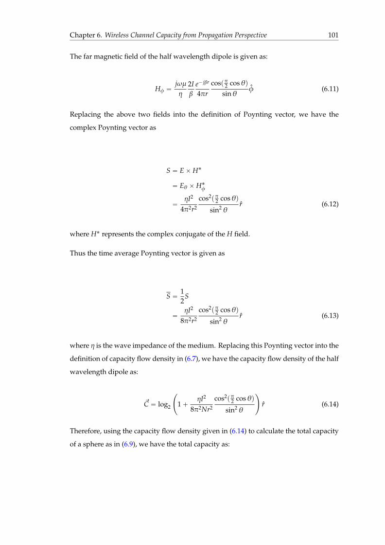
Chapter 6. Wireless Channel Capacity from Propagation Perspective 101
The far magnetic field of the half wavelength dipole is given as:
Hφ “jωµη
2Iβ
e´ jβr
4πrcospπ2 cosθq
sinθφ (6.11)
Replacing the above two fields into the definition of Poynting vector, we have the
complex Poynting vector as
S “ EˆH˚
“ Eθ ˆH˚φ
“ηI2
4π2r2
cos2pπ2 cosθq
sin2 θr (6.12)
where H˚ represents the complex conjugate of the H field.
Thus the time average Poynting vector is given as
S “12
S
“ηI2
8π2r2
cos2pπ2 cosθq
sin2 θr (6.13)
where η is the wave impedance of the medium. Replacing this Poynting vector into the
definition of capacity flow density in (6.7), we have the capacity flow density of the half
wavelength dipole as:
~C “ log2
˜
1`ηI2
8π2Nr2
cos2pπ2 cosθq
sin2 θ
¸
r (6.14)
Therefore, using the capacity flow density given in (6.14) to calculate the total capacity
of a sphere as in (6.9), we have the total capacity as:

Chapter 6. Wireless Channel Capacity from Propagation Perspective 102
C “S
~C ¨ d~s
“
S
log2
˜
1`ηI2
8π2Nr2
cos2pπ2 cosθq
sin2 θ
¸
r ¨ d~s
“
ż 2π
0
ż π
0log2
˜
1`ηI2
8π2Nr2
cos2pπ2 cosθq
sin2 θ
¸
r2 sin2 θdθdφ
“ 2πr2ż π
0log2
˜
1`ηI2
8π2Nr2
cos2pπ2 cosθq
sin2 θ
¸
sinθdθ (6.15)
where S denotes the surface of the sphere.
The above equation is the total capacity of a sphere with a half wavelength dipole at the
centre. As the integral in the equation does not have a simple closed form, we resort
to numerical integration to obtain the results. We calculate the total capacity of sphere
with other types of sources in this section before we present the numerical integration
results in Section 6.8.
6.4.1.2 Total Capacity of a Sphere with 2-element Linear Array
In this section, we consider a uniform linear array antenna as the radiating source and
calculate the total capacity of a sphere. The linear array we consider is a 2-element
array. Each element is a half wavelength dipole antenna with one wavelength apart.
According to the array multiplication principle [105], the E field and H field of the array
are the E field and H field of the element antenna multiplied by the array factor. Thus,
the fields can be written as:
Earray “ Esingle f pθ, φq (6.16)
Harray “ Hsingle f pθ, φq (6.17)
where f pθ, φq is the normalised array factor; Earray and Harray are the fields of the array
antenna and Esingle and Hsingle are the fields of the element antenna.

Chapter 6. Wireless Channel Capacity from Propagation Perspective 103
We assume a simple 2-element array with one wavelength apart. Thus, the array factor
is given as [105] :
f pθq2element “ cospπ cosθq (6.18)
We assume a 2-element array antenna with each element a half wavelength dipole
antenna. With the fields of the element of half wavelength dipole given in (6.10) and
(6.11), we the fields of the 2-element half wavelength dipole array antenna as:
E2element “ jωµ2Iβ
e´ jβr
4πrcospπ2 cosθq
sinθcospπ cosθqθ (6.19)
H2element “jωµη
2Iβ
e´ jβr
4πrcospπ2 cosθq
sinθcospπ cosθqφ (6.20)
With the field values, we have the capacity flow density of the 2-element array as:
~C2element “ log2
˜
1`ηI2
8π2Nr2
cos2pπ2 cosθq cos2pπ cosθq
sin2 θ
¸
r (6.21)
Thus the total capacity follows as:
C2element “
~C2element ¨ d~s
“ 2πr2ż π
0log2
˜
1`ηI2
8π2Nr2
cos2pπ2 cosθq cos2pπ cosθq
sin2 θ
¸
sinθdθ (6.22)
Again the total capacity is an integral form.
6.4.1.3 4-element array
To further see the effects of the array antenna, we adopt a 4-element uniform linear array
antenna with each element a half wavelength dipole antenna. The distance between
each element is one wavelength. The array geometry is shown in Figure 6.2.

Chapter 6. Wireless Channel Capacity from Propagation Perspective 104
Figure 6.2: Array Geometry of a 4-element Uniform Linear Array
Following the array multiplication principle in [105], the total array factor is written as:
AF “ Ie jβ d2 cosθ ` Ie´ jβ d
2 cosθ ` Ie jβ 3d2 cosθ ` Ie´ jβ 3d
2 cosθ (6.23)
where d is the distance between the array elements. In our case, d “ λ.
The array factor can be further simplified and normalised. The normalised array factor
is given as:
f pθq4element “ cospπ cosθq cosp2π cosθq (6.24)
Again, using this array factor, we have the capacity flow density of the array as:
~C4element “ log2
˜
1`ηI2
8π2Nr2
cos2pπ2 cosθq cos2pπ cosθq cos2p2π cosθq
sin2 θ
¸
r (6.25)
And the total capacity is:
C4element “
~C4element ¨ d~s (6.26)
“ 2πr2ż π
0log2
˜
1`ηI2
8π2Nr2
cos2pπ2 cosθq cos2pπ cosθq cos2p2π cosθq
sin2 θ
¸
sinθdθ
(6.27)
6.4.1.4 Total Capacity of An Isotropic Source
For comparison purpose, we also look into the total capacity of an isotropic radiating
source. An isotropic source is a source that radiates power uniformly in all the spatial

Chapter 6. Wireless Channel Capacity from Propagation Perspective 105
directions. It is an idealised radiating source. It is used as a basis for comparing the
radiation performance of a specific antenna.
We first compute the power flow density of an isotropic source which has the same total
radiating power as a half wavelength dipole antenna.
With the Poynting vector given in (6.12), the total radiating power of a half wavelength
dipole antenna is given as:
Pt “
S
~S ¨ d~s
“
ż π
0
ηI2
2πcos2pπ2 cosθq
sinθdθ (6.28)
Following the assumption that the isotropic source radiating the power uniformly into
all the spatial direction, the power flow density is given as the total radiating power
averaged over a uniform sphere. Thus, it is given as:
~Siso “Pt
4πr2~r
“
ż π
0
ηI2
8π2r2
cos2pπ2 cosθqsinθ
dθ~r (6.29)
The integral result of the equation
ż π
0
cos2pπ2 cosθqsinθ
dθ “12p´Cip2πq ` γ` lnp2πqq (6.30)
where Cip˚q is the cosine integral function and γ is the Euler-Mascheroni constant. Thus,
the final result of the above integral is:
ż π
0
cos2pπ2 cosθqsinθ
dθ « 1.2188 (6.31)
Thus the Poynting vector of the isotropic source can be written as:

Chapter 6. Wireless Channel Capacity from Propagation Perspective 106
~Siso “ 0.6094ηI2
4π2r2~r (6.32)
This is the power flow density vector of an isotropic source which has the same amount
of radiating power Pt as the half wavelength dipole. We will use this equivalent power
isotropic antenna to compare with other realistic radiation sources.
Following the definition of the capacity flow density, we replace (6.32) to the definition
of capacity flow density. The resulting capacity flow density of an isotropic source is
thus written as:
~Ciso “ log2
˜
1` 0.6094ηI2
4π2r2N
¸
~r (6.33)
Similarly, using this capacity flow density, the total capacity of the isotropic source is
thus given as:
Ciso “
*S
~Ciso ¨ ds
“ 4πr2 log2
˜
1` 0.6094ηI2
4π2r2N
¸
(6.34)
Until now, we have the integral forms of total capacity of a sphere of 4 types of sources:
half wavelength dipole; 2-element dipole array; 4-element linear dipole array and
equivalent isotropic source. However, the results involve complex integral forms. We
will present numerical integral results in the next section.
6.4.2 Total Capacity of Sphere with A Non-central Source
It is an ideal assumption that the radiating source is always at the centre of the sphere.
In this section, we calculate the total capacity of a sphere shape volume space when the
radiating source is not at the centre of the sphere. We study the influence of the location
of the source inside the sphere has on the total capacity of the sphere.

Chapter 6. Wireless Channel Capacity from Propagation Perspective 107
X
Y
Z
P
dr
p
q
Figure 6.3: Geometry of a Sphere with a Non-centre Source
First we assume the location of the source is at the location pp, 0, 0q in the spherical
coordinate system. The sphere has the origin as the location p0, 0, 0q. The geometry is
illustrated in Figure 6.3.
Based on the geometry in Figure 6.3, we have the following relationship:
d2 “ r2 cos2 θ` q2
where d is the distance from the source to a certain point on the sphere surface; r is the
radius of the sphere; and q is given in the following equation according to the according
to the law of cosine.
q2 “ p2 ` r2 sin2 θ` 2pr sinθ sinφ (6.35)
Thus, we obtain the distance from the source at pp, 0, 0q to a certain point on the sphere
surface as:
d “b
r2 ` p2 ` 2rp sinθ sinφ (6.36)
Then we replace this distance into the capacity flow density in (6.14), (6.21), (6.25) and
(6.33), we have the capacity flow density with the radiating source at the location of
pp, 0, 0q for the 4 types of sources that we have derived for centre location as:

Chapter 6. Wireless Channel Capacity from Propagation Perspective 108
~C “ log2
˜
1`ηI2
8π2Npr2 ` p2 ` 2rp sinθ sinφq
cos2pπ2 cosθq
sin2 θ
¸
r (6.37)
~C2element “ log2
˜
1`ηI2
8π2Npr2 ` p2 ` 2rp sinθ sinφq
cos2pπ2 cosθq cos2pπ cosθq
sin2 θ
¸
r
(6.38)
~C4element “ log2
˜
1`ηI2
8π2Npr2 ` p2 ` 2rp sinθ sinφq
cos2pπ2 cosθq cos2pπ cosθq cos2p2π cosθq
sin2 θ
¸
r
(6.39)
~Ciso “ log2
˜
1` 0.6094ηI2
4π2Npr2 ` p2 ` 2rp sinθ sinφq
¸
~r (6.40)
The four equations in (6.37), (6.38), (6.39) and (6.40) are the capacity flow density for the
half wavelength dipole, 2-element dipole array, 4-element linear dipole array and the
equivalent isotropic source, respectively, with the source located at pp, 0, 0q.
Thus, by integrating the capacity flow density over the sphere surface, we have the total
capacity of the sphere with the source at the location of pp, 0, 0q as:
Cpr, pqdipole “
ż 2π
0
ż π
0log2
˜
1`ηI2
8π2Npr2 ` p2 ` 2rp sinθ sinφq
cos2pπ2 cosθq
sin2 θ
¸
r2 sin2 θdθdφ
(6.41)
Cpr, pq2element “
ż 2π
0
ż π
0log2p1`
ηI2
8π2Npr2 ` p2 ` 2rp sinθ sinφqcos2pπ2 cosθq cos2pπ cosθq
sin2 θqr2 sin2 θdθdφ (6.42)

Chapter 6. Wireless Channel Capacity from Propagation Perspective 109
Cpr, pq4element “
ż 2π
0
ż π
0log2p1`
ηI2
8π2Npr2 ` p2 ` 2rp sinθ sinφqcos2pπ2 cosθq cos2pπ cosθq cos2p2π cosθq
sin2 θqr2 sin2 θdθdφ (6.43)
Ciso “
ż 2π
0
ż π
0log2
˜
1` 0.6094ηI2
4π2Npr2 ` p2 ` 2rp sinθ sinφq
¸
r2 sin2 θdθdφ (6.44)
The above 4 equations in (6.41), 6.42), (6.43) and (6.44) are the total capacity calculation
equations of the half wavelength dipole antenna, the 2-element dipole antenna array,
the 4-element dipole antenna array and the equivalent isotropic source, respectively,
with the location at pp, 0, 0q. We write the total capacity as a function of both the sphere
radius r and the shift from the origin p. Again, the total capacity involves an integral
form. The numerical integral results are presented in Section 6.8.
6.5 Properties of Capacity of A Sphere
We have derived the integral forms of the total capacity of 4 types of sources both at
the centre location and the non-centre location of the sphere. The numerical integral
results will be presented in Section 6.8. However, we have two important general results
concerning the total capacity of sphere.
The first property is a general result of the total capacity of sphere concerning the
antenna types.
Proposition 6.2. Among the sources placed at the centre of the sphere, the isotropic radiating
source has the maximum total capacity.
Proof. For simplicity we can write the Poynting vector of an arbitrary source as in [105]:
Upθ, φq “ Dpθ, φqUave (6.45)

Chapter 6. Wireless Channel Capacity from Propagation Perspective 110
where Dpθ, φq is the directive gain; Uave is the radiating intensity of an isotropic source
and Upθ, φq is the radiating intensity defined as:
Upθ, φq “ ~S ¨ r2~r (6.46)
Replacing (6.46) into (6.45), we have the Poynting vector as:
~S “ Dpθ, φq~Save (6.47)
where ~Save is the Poynting vector of an isotropic source defined as:
~Save “Pr
4πr2~r (6.48)
Therefore, following the capacity flow density in (6.7), we have the capacity flow density
as:
~C “ log2
ˆ
1`PrDpθ, φq
4πNr2
˙
~r (6.49)
and the total capacity as:
C “ 2πr2ż π
0log2
ˆ
1`PrDpθ, φq
4πNr2
˙
sinθdθ (6.50)
Under the condition that the directive gain is between 0 and 1:
0 ď Dpθ, φq ď 1
, we obtain the maximum of the the total capacity in (6.50) when Dpθ, φq “ 1 for all the
spatial angle of θ which is equivalent to isotropic radiation as:

Chapter 6. Wireless Channel Capacity from Propagation Perspective 111
C “ 2πr2ż π
0log2
ˆ
1`PrDpθ, φq
4πNr2
˙
sinθdθ
ď 2πr2ż π
0log2
ˆ
1`Pr
4πNr2
˙
sinθdθ
“ 4πr2 log2
ˆ
1`Pr
4πNr2
˙
“ Ciso (6.51)
This concludes the proof.
The second property is concerning the location of the source in a sphere. We have the
following proposition:
Proposition 6.3. For a source at a distance shift p from the origin of the sphere, among the
distance shifts p, where 0 ď p ď r, when p “ 0, which means the source is at the centre of the
sphere, the total capacity has the maximum value.
Proof. Replacing the geometry relation in (6.36) into the total capacity in (6.50), we have
the total capacity as a function of p as:
Cppq “ 2πr2ż π
0log2
ˆ
1`PrDpθ, φq
4πNpr2 ` p2 ` 2pr cosθq
˙
sinθdθ (6.52)
Taking derivative of the function Cppqwe have:
dCppqdp
“ddp
ˆ
log2
ˆ
1`PrDpθ, φq
4πNpr2 ` p2 ` 2pr cosθq
˙
sinθdθ˙
“ ´2πr2ż π
0
p2p` 2r cosθqPrDpθ, φq4πNpr2 ` p2 ` 2pr cosθq2 ` PrDpθ, φqpr2 ` p2 ` 2pr cosθq
dθ
(6.53)
The condition to find the maximum value of function Cppq is to set the derivative of
Cppq as zero :dCppq
dp“ 0

Chapter 6. Wireless Channel Capacity from Propagation Perspective 112
.
Thus, by setting the capacity derivative in (6.53) as zero, we have the following condi-
tion:
p “ ´r cosθ (6.54)
Under the condition that p is a non-negative value; and r is a non-zero value, with
0 ď θ ď π, the value to achieve the condition in (6.54) is cosθ “ 0, which results in
p “ 0.
This concludes the proof.
6.6 Calculating the Total Capacity using Divergence
The total capacity of an enclosed volume space is defined as the total capacity flow
density flux flowing through the enclosed surface. Following this definition, we have
calculated the capacity of a sphere shape volume capacity containing a radiating source
in the last section. However, in applications the shape of the volume space is not a perfect
sphere, which leads to difficulty in deriving the integral form of the total capacity. In
this section, we present an alternative method of calculating the total capacity of an
enclosed volume space by applying the divergence theorem to the definition of the total
capacity.
The total capacity of an enclosed volume space is defined as the total capacity flow
density flux flowing through the total surface area in (6.9).
Under the assumption that the volume space is enclosed, applying the divergence
thorem to this definition, we arrive at:
S
~C ¨ d~s “$
V
p∇ ¨ ~Cqdv (6.55)
where ∇ ¨ ~C is the divergence of the capacity flow density.

Chapter 6. Wireless Channel Capacity from Propagation Perspective 113
This equation provides an alternative method of calculating the total capacity of an
enclosed volume space via calculating the divergence of the capacity flow density.
While divergence of the capacity flow density is crucial in applying this method, we
first study the divergence of the capacity flow density with the 4 types of sources we
have used in Section 6.4.
6.6.1 Divergence of Various Sources
As the divergence of the capacity flow density field is the key to use the divergence
theorem to calculate the total capacity, we first compute the divergence of various
sources in this section.
6.6.1.1 Divergence of Half Wavelength Dipole Antenna
The capacity flow density of the half wavelength dipole is given in (6.14). Following
the definition of divergence of a vector A in spherical coordinate system as [106]:
∇ ¨ ~A “1r2B
Brpr2Arq `
1r sinθ
B
BθpsinθAθq `
1r sinθ
BAφ
Bφ(6.56)
where Ar, Aθ and Aφ are the three vector components of vector A in the spherical
coordinate system. For the capacity flow density in our case, the capacity flow density
in the far field only has a component in the ~r direction. Thus the divergence of the
capacity flow density is given as:
∇ ¨ ~C “1r2B
Brpr2Crq
“1r2 p2rCr ` r2 BCr
Brq
“2Cr
r`BCr
Br(6.57)
where Cr is the capacity flow density in the ~r direction.
We use this equation in the calculation of the divergence of capacity flow density of
various sources. Applying the above (6.57) to the capacity flow density of the 4 types

Chapter 6. Wireless Channel Capacity from Propagation Perspective 114
of the sources in (6.14), (6.21), (6.25) and (6.33), we have the divergence of the capacity
flow density of the 4 types of sources as:
∇ ¨ ~Cdipole “2r
log2
˜
1`ηI2
4π2r2Ncos2pπ2 cosθq
sin2 θ
¸
´2η I2
N cos2pπ2 cosθq
4π2r3 sin2 θ` η I2
N r cos2p I2
N cosθq(6.58)
∇ ¨ ~C2element “2r
log2
˜
1`ηI2
4π2r2Ncos2pπ2 cosθq cos2pπ cosθq
sin2 θ
¸
´2η I2
N cos2pπ2 cosθq cos2pπ cosθq
4π2r3 sin2 θ` η I2
N r cos2p I2
N cosθq cos2pπ cosθq(6.59)
∇ ¨ ~C4element “2r
log2
˜
1`ηI2
4π2r2Ncos2pπ2 cosθq cos2pπ cosθq cos2p2π cosθq
sin2 θ
¸
´2η I2
N cos2pπ2 cosθq cos2pπ cosθq cos2p2π cosθq
4π2r3 sin2 θ` η I2
N r cos2p I2
N cosθq cos2ppi cosθq cos2p2π cosθq(6.60)
∇ ¨ ~Cisotropic “2r
log2
˜
1` 0.6094ηI2
4π2r2N
¸
´1.288η I2
N
4π2r3 sin2 θ` 0.6094η I2
N r(6.61)
The above divergence results in (6.58), (6.59), (6.60) and (6.61) are the divergence of
capacity flow density of half wavelength dipole antenna, 2-element dipole array, 4-
element dipole uniform linear array and the equivalent isotropic source, respectively.
Except the isotropic source, the divergence of the rest 3 sources depends on both the
distance r and the angle θ. We plot the divergence of the half wavelength dipole in
Figure 6.4 as a 3D surface as a function of both the distance r and the angle θ, where theI2
N “ 5.

Chapter 6. Wireless Channel Capacity from Propagation Perspective 115
Figure 6.4: 3D Plot of the Divergence of a Half-wavelength Dipole Antenna
1 2 3 4 5 6 7 8 9 10
Distance from Source in metres
0
2
4
6
8
10
12
14
Div
erge
nce
Val
ue in
bits
/s/m
2
Isotropic SourceHalf Wavelength Dipole
Figure 6.5: Divergence Values of Half-wavelength Dipole and Isotropic Source whenθ “ 0
In Figure 6.5, we plot the divergence of all the 4 types of source against the distance r
by fixing the angle θ “ 0.
From both Figure 6.4 and Figure 6.5, we see that the divergence of the capacity flow
density is a function of the distance r. After dropping from the peak near the source, it
still extends with the distance fairly far from the source. If we see the divergence of the
capacity flow density as a ’source’ of the capacity, then this explains the total capacity
increase with the volume space as the ’source’ extends with the distance extends. In the

Chapter 6. Wireless Channel Capacity from Propagation Perspective 116
next section, we use the divergence of the capacity flow density to calculate the total
capacity of an enclosed volume space of cube shape.
6.7 Total Capacity of A Cube
In Section 6.4 we calculated the total capacity of an enclosed volume space of perfect
sphere shape. However, in practical applications, it is rare that the interested design
space is a perfect sphere. For example, in indoor wireless network design, the shape
of indoor rooms is often cuboid. To gain an insight of the influence of the shape of the
volumes space on the total capacity, in this section, we calculate the total capacity of
a cube shaped volume space. Different from the sphere shaped volume space, where
the integral of capacity flow density is performed over the perfect sphere shape, the
irregularity of the cube surface leads to difficulty in obtaining the integral form of the
capacity flow density over the cube surface. Therefore, we resort to the method of
divergence introduced in Section 6.6 to calculate the total capacity of a cube. Similar to
the sphere case, we also calculated the 4 types of sources at the centre of the cube and
at the non-centre of the cube. We use the divergence of the 4 types of source computed
in Section 6.6 to calculate the total capacity in this case.
6.7.1 Total Capacity of A Cube with Centre Source
In this section, we derive the mathematical form of the total capacity of a cube shaped
enclosed volume space with the source at the centre of the cube.
We assume a cube with the edge length 2a with the original of the Cartesian coordinate
system at the centre of the cube. The radiating source is also placed at the centre of the
cube. The geometry is illustrated in Figure 6.6.
The divergence of the 4 types of source given in (6.58), (6.59), (6.60) and (6.61) are in
the form of spherical coordinate system. In our calculation, it is desirable to convert to
the Cartesian coordinate system to integral the cube volume space. The transformation
from the spherical coordinate system to the Cartesian coordinate system utilises the
following identities:

Chapter 6. Wireless Channel Capacity from Propagation Perspective 117
X
Y
Z
2a
Figure 6.6: Geometry of Cube-Shaped Volume Space
r “b
x2 ` y2 ` z2 (6.62)
cosθ “z
a
x2 ` y2 ` z2(6.63)
sinθ “
a
x2 ` y2a
x2 ` y2 ` z2(6.64)
Replacing (6.64) in (6.58), (6.59), (6.60) and (6.61) yields the divergence of the 4 types of
sources in the Cartesian coordinate system as:
Dpx, y, zqdipole “2
a
x2 ` y2 ` z2log2
¨
˝1`ηI2 cos2pπ2
z?x2`y2`z2
q
4π2px2 ` y2qN
˛
‚
´
2η I2
N cos2pπ2z?
x2`y2`z2q
4π2px2 ` y2qa
x2 ` y2 ` z2 ` η I2
N
a
x2 ` y2 ` z2 cos2pπ2z?
x2`y2`z2q
(6.65)
Dpx, y, zq2element “2
a
x2 ` y2 ` z2log2
ˆ
1`Fpx, y, zq2element
4π2px2 ` y2q
˙
´2Fpx, y, zq2element
4π2px2 ` y2qa
x2 ` y2 ` z2 ` Fpx, y, zq2element(6.66)

Chapter 6. Wireless Channel Capacity from Propagation Perspective 118
Dpx, y, zq4element “2
a
x2 ` y2 ` z2log2
ˆ
1`Fpx, y, zq4element
4π2px2 ` y2q
˙
´2Fpx, y, zq4element
4π2px2 ` y2qa
x2 ` y2 ` z2 ` Fpx, y, zq4element(6.67)
Dpx, y, zqisotropic “2
a
x2 ` y2 ` z2log2
˜
1` 0.6094ηI2
4π2px2 ` y2 ` z2qN
¸
´1.288η I2
N
4π2pa
x2 ` y2 ` z2q3 ` 0.6094η I2
N
a
x2 ` y2 ` z2(6.68)
where
Fpx, y, zq2element “ ηI2
N
b
x2 ` y2 ` z2 cos2pπ2
za
x2 ` y2 ` z2q cos2pπ
za
x2 ` y2 ` z2q
(6.69)
Fpx, y, zq4element “η
NI2 cos2p
π2
za
x2 ` y2 ` z2q cos2pπ
za
x2 ` y2 ` z2q cos2p2π
za
x2 ` y2 ` z2q
(6.70)
The divergence values Dpx, y, zq in the above equations in (6.65), (6.66), (6.67) and (6.68)
are written as a function of the Cartesian coordinate location px, y, zq which represents
the divergence at the location px, y, zq. Following the divergence method of calculating
the total capacity in (6.55), we have the total capacity of the 4 types of sources as:

Chapter 6. Wireless Channel Capacity from Propagation Perspective 119
Cdipole “
$V
Dpx, y, zqdipoledv
“
ż a
´a
ż a
´a
ż a
´aDpx, y, zqdipoledxdydz
“
ż a
´a
ż a
´a
ż a
´a
2a
x2 ` y2 ` z2log2
¨
˝1`ηI2 cos2pπ2
z?x2`y2`z2
q
4π2px2 ` y2qN
˛
‚
´
2η I2
N cos2pπ2z?
x2`y2`z2q
4π2px2 ` y2qa
x2 ` y2 ` z2 ` η I2
N
a
x2 ` y2 ` z2 cos2pπ2z?
x2`y2`z2qdxdydz
(6.71)
C2element “
$V
Dpx, y, zq2elementdv
“
ż a
´a
ż a
´a
ż a
´aDpx, y, zq2elementdxdydz
“
ż a
´a
ż a
´a
ż a
´a
2a
x2 ` y2 ` z2log2
ˆ
1`Fpx, y, zq2element
4π2px2 ` y2q
˙
´2Fpx, y, zq2element
4π2px2 ` y2qa
x2 ` y2 ` z2 ` Fpx, y, zq2elementdxdydz (6.72)
C4element “
$V
Dpx, y, zq4elementdv
“
ż a
´a
ż a
´a
ż a
´aDpx, y, zq4elementdxdydz
“
ż a
´a
ż a
´a
ż a
´a
2a
x2 ` y2 ` z2log2
ˆ
1`Fpx, y, zq4element
4π2px2 ` y2q
˙
´2Fpx, y, zq4element
4π2px2 ` y2qa
x2 ` y2 ` z2 ` Fpx, y, zq4elementdxdydz (6.73)

Chapter 6. Wireless Channel Capacity from Propagation Perspective 120
Cisotropic “
$V
Dpx, y, zqisotropicdv
“
ż a
´a
ż a
´a
ż a
´aDpx, y, zqisotropicdxdydz
“
ż a
´a
ż a
´a
ż a
´a
2a
x2 ` y2 ` z2log2
˜
1` 0.6094ηI2
4π2px2 ` y2 ` z2qN
¸
´1.288η I2
N
4π2pa
x2 ` y2 ` z2q3 ` 0.6094η I2
N
a
x2 ` y2 ` z2dxdydz (6.74)
The above equations in (6.71), (6.72), (6.73) and (6.74) give the total capacity of a cube
shape with the half wavelength dipole, 2-element dipole array, 4-element uniform linear
dipole array and the equivalent isotropic source, respective, all at centre of the cube.
The results require multiple integrals. We will present the numerical integration results
in the later section.
6.7.2 Total Capacity of Cube with Non-Centre Source
Same as the sphere shaped volume space case, we also calculate the total capacity of
the cube with the sources at the non-centre location. We assume that the location of the
source is shifted to the location of pp, 0, 0q in Cartesian coordinate system. According to
the total capacity results in a multiple integral form in (6.71), (6.72), (6.73) and (6.74), the
total capacity of the source at pp, 0, 0q results only a shift in one dimension of the integral
limits fromşa´a to
şa`p´a`p. Thus it is straightforward to have the following integral forms
of the total capacity of the 4 types of sources at location pp, 0, 0q as:
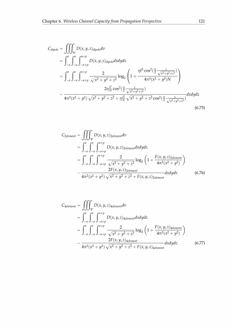
Chapter 6. Wireless Channel Capacity from Propagation Perspective 121
Cdipole “
$V
Dpx, y, zqdipoledv
“
ż a
´a
ż a
´a
ż a`p
´a`pDpx, y, zqdipoledxdydz
“
ż a
´a
ż a
´a
ż a`p
´a`p
2a
x2 ` y2 ` z2log2
¨
˝1`ηI2 cos2pπ2
z?x2`y2`z2
q
4π2px2 ` y2qN
˛
‚
´
2η I2
N cos2pπ2z?
x2`y2`z2q
4π2px2 ` y2qa
x2 ` y2 ` z2 ` η I2
N
a
x2 ` y2 ` z2 cos2pπ2z?
x2`y2`z2qdxdydz
(6.75)
C2element “
$V
Dpx, y, zq2elementdv
“
ż a
´a
ż a
´a
ż a`p
´a`pDpx, y, zq2elementdxdydz
“
ż a
´a
ż a
´a
ż a`p
´a`p
2a
x2 ` y2 ` z2log2
ˆ
1`Fpx, y, zq2element
4π2px2 ` y2q
˙
´2Fpx, y, zq2element
4π2px2 ` y2qa
x2 ` y2 ` z2 ` Fpx, y, zq2elementdxdydz (6.76)
C4element “
$V
Dpx, y, zq4elementdv
“
ż a
´a
ż a
´a
ż a`p
´a`pDpx, y, zq4elementdxdydz
“
ż a
´a
ż a
´a
ż a`p
´a`p
2a
x2 ` y2 ` z2log2
ˆ
1`Fpx, y, zq4element
4π2px2 ` y2q
˙
´2Fpx, y, zq4element
4π2px2 ` y2qa
x2 ` y2 ` z2 ` Fpx, y, zq4elementdxdydz (6.77)

Chapter 6. Wireless Channel Capacity from Propagation Perspective 122
Cisotropic “
$V
Dpx, y, zqisotropicdv
“
ż a
´a
ż a
´a
ż a`p
´a`pDpx, y, zqisotropicdxdydz
“
ż a
´a
ż a
´a
ż a`p
´a`p
2a
x2 ` y2 ` z2log2
˜
1` 0.6094ηI2
4π2px2 ` y2 ` z2qN
¸
´1.288η I2
N
4π2pa
x2 ` y2 ` z2q3 ` 0.6094η I2
N
a
x2 ` y2 ` z2dxdydz (6.78)
6.8 Numerical Results
In this section, we present the numerical integral results for the total capacity forms
derived in Section 6.4 and Section 6.7. The results are also presented in two parts: the
sphere shaped volume space case and the cube-shaped volume space case.
6.8.1 Total Capacity of A Sphere
The total capacity values for 4 types of sources at centre derived in (6.15), (6.22), (6.27)
and (6.34) are plotted a function of the sphere radius r in Figure 6.7.
The value of PN can be seen as an equivalence to the signal-to-noise ratio (SNR). In the
numerical integral calculation, we choose two values for the SNR1 “ 5 and SNR2 “ 10.
The total capacity values show that the isotropic source has the largest value among the
4 types of sources as we have proved in Proposition 6.2.
The total capacity values of the 4 types sources at non-centre location derived in (6.41),
(6.42), (6.43) and (6.44) are plotted in Figure 6.8.
Under the SNR condition set as SNR “ 5, the total capacity values of the 4 types of
sources are plotted against the sphere radius r in two locations p “ 1 and p “ 2. The
numerical results show that the total capacity values increase with the radius r and the
sources at the location p “ 1 have higher total capacity than the sources at the location
p “ 2.

Chapter 6. Wireless Channel Capacity from Propagation Perspective 123
1 2 3 4 5 6 7 8 9 10
sphere radiance r (metres)
0
100
200
300
400
500
600
700
800
900
tota
l cap
acity
C (
bits
/sec
)
isotropic source SNR=5half wavelength dipole SNR=52 element array SNR54 element array SNR=5isotropic source SNR=10half wavelength dipole SNR=102 element array SNR=104 element array SNR=10
Figure 6.7: Total Capacity of Sphere with Centre Source Vs Sphere Radius
2 3 4 5 6 7 8 9 10
sphere radiance r (metres)
0
50
100
150
200
250
300
350
400
450
500
tota
l cap
acity
C (
bits
/sec
)
isotropic source p=1 metrehalf wavelength dipole p=1 metre2 element array p=1 metre4 element array p=1 metreisotropic source p=2 metreshalf wavelength dipole p=2 metres2 element array p=2 metres4 element array p=2 metres
Figure 6.8: Total Capacity of Sphere with Non-centre Source Vs Sphere Radius

Chapter 6. Wireless Channel Capacity from Propagation Perspective 124
0 1 2 3 4 5 6 7 8 9 10
distance from origin p (metres)
0
100
200
300
400
500
600
tota
l cap
acity
C (
bits
/sec
) isotropic source r=25 metreshalf wavelength dipole r=25 metres2 element array r=25 metres4 element array r=25 metresisotropic source r=15 metreshalf wavelength dipole r=15 metres2 element array r=15 metres4 element array r=15 metres
Figure 6.9: Total Capacity of Sphere with Non-Centre Source Vs Shift Distance
The total capacity values are also plotted against the distance from the origin p in
Figure 6.9. The total capacity values decrease with the distance p as we have proved in
Proposition 6.3.
6.8.2 Total Capacity of A Cube
The numerical results of the total capacity of a cube-shaped volume space with a centre
source derived in (6.71), (6.72), (6.73) and (6.74) are plotted as a function of half the
cube-edge length l in Figure 6.10. The SNR are set as SNR1 “ 5 and SNR2 “ 10.
The numerical results of the total capacity show similar pattern as in the sphere-shaped
case. The total capacity increase with the total volume space and the isotropic source
has the largest total capacity.
The numerical results of the total capacity with a non-centre source derived in (6.75),
(6.76), (6.77) and (6.78) are plotted in Figure 6.11. The SNR is set as SNR “ 5 and the
positions of the source are chosen as p “ 1 and p “ 2.
Again, the numerical values of the total capacity show similar pattern as in the sphere
case. The nearer position to the centre (p=1) has a larger total capacity than the farther

Chapter 6. Wireless Channel Capacity from Propagation Perspective 125
1 2 3 4 5 6 7 8 9 10
half edge length l (metres)
0
200
400
600
800
1000
1200
1400
Tot
al c
apac
ity C
(bi
ts/s
ec)
isotropic source SNR1half wavelength dipole SNR1half wavelength array SNR14 element array SNR1isotropic source SNR2half wavelength dipole SNR2half wavelength array SNR24 element array SNR2
Figure 6.10: Total Capacity of Cube with Centre Source Vs Cube Edge Length
0 1 2 3 4 5 6 7 8
half edge length l (metres)
0
100
200
300
400
500
600
700
800
tota
l cap
acity
C (
bits
/sec
)
isotropic source p=1 metrehalf wavelength dipole p=1 metrehalf wavelength array p=1 metre4 element array p=1 metreisotropic source p=2 metreshalf wavelength dipole p=2 metreshalf wavelength array p=2 metres4 element array p=2 metres
Figure 6.11: Total Capacity of Cube with Non-Centre Source Vs Cube Edge Length

Chapter 6. Wireless Channel Capacity from Propagation Perspective 126
0 1 2 3 4 5 6 7 8 9 10
the distance shift p (metres)
0
100
200
300
400
500
600
700
800
tota
l cap
acity
C (
bits
/sec
)isotropic source l=10 metershalf wavelength dipole l=10 metreshalf wavelength array l=10 metres4 element array l=10 metresisotropic source l=5 metreshalf wavelength dipole l=5 metreshalf wavelength array l=5 metres4 element array l=5 metres
Figure 6.12: Total Capacity of Cube with Non-centre Source Vs Shift Distance
position (p=2). The numerical values of the total capacity are also plotted against the
distance from the centre in Figure 6.12.
The results again show similar pattern as in the sphere case. The centre position has the
largest total capacity of a cube-shaped volume space.
6.9 Discussion and Conclusion
From the integral forms of total capacity derived in Section 6.4 and Section 6.7 and the
numerical results in Section 6.8, we have the following conclusions regarding the total
capacity of a volume space :
6.9.1 The total capacity increases with the space volume
From both the sphere and cube case, the total capacity increases with the space volume,
even with a fixed transmitter power. This result suggests that the capacity of a wireless

Chapter 6. Wireless Channel Capacity from Propagation Perspective 127
channel can always be increased through the increase of the usable spatial degree-of-
freedom. Even with a limited transmit power, spreading the power into more degree-
of-freedom always results in a positive capacity gain.
6.9.2 Isotropic radiating source has largest total capacity
Conventional antenna design aims to achieve highly directive transmitter antenna by
using array, which is based on the point-to-point communication model. However,
this conclusion offers an sight to the capacity of wireless channel and the design of
communication EM radiating system. To improve the total capacity, it is desirable to
spread the total transmitter power into more spatial degree-of-freedom.
6.9.3 Conclusion
In this work, we study the wireless channel capacity limit from electromagnetic per-
spective. We establish a capacity flow density field based on the power flow density
and the classic AWGN channel capacity. Based on the capacity flow density we in-
troduced a new wireless channel capacity limit of volume space, by incorporating the
continuous electromagnetic field to study the conventional discrete point-based com-
munication channel. Our results of the total capacity of enclosed volume space show
that the capacity of wireless channel always gains through the abundance of the space
volume.
The main contribution of this chapter is to calculate the wireless channel capacity of
an enclosed volume space. Although the MIMO communication theory proved the
number of antennas commands the channel capacity of a MIMO system, the impact
of spatial volume on the wireless channel capacity was unknown before this work. In
this chapter, the numerical calculation results quantify the amount of wireless channel
capacity which a certain spatial volume can support. The results showed that the larger
volume space supports higher channel capacity. Such results corroborate the general
conclusion of wireless communications that spatial degree-of-freedoms can increase
wireless channel capacity.

Chapter 7
Conclusion and Future Work
7.1 Conclusion
In this chapter, I conclude the PhD research project on channel modelling for wireless
network planning. I further discuss the limitation of the research presented in this
project and presented potential future research directions.
In this PhD research project, I developed advanced channel models for 5G wireless
network planning and optimisation. The focus is on massive MIMO channel, mmWave
channel and distributed MIMO. Based on traditional ray launching simulation, site-
specific channel models are developed for network planning and optimisation ap-
plications. Traditional ray launching simulation has been shown to be extended to
accommodate the 5G network techniques and still effective in channel map construc-
tion. A new model calibration method is also developed and shown to be effective
when measurement is available. Furthermore a wireless channel capacity concept from
electromagnetic propagation perspective is defined and demonstrated to have potential
application network planning and optimisation.
For massive MIMO system, the large number of antenna array posed computational
complexity barrier on the physical channel modelling. However, the analysis in this
project showed that the physical model can be simplified by utilising the geometry of
the large antenna arrays in the massive MIMO systems.
128

Chapter 5. Conclusion and Future Work 129
For mmWave channels, the high free space propagation loss can be exploited to develop
efficient channel models. In this project, a path loss model for mmWave channel is
developed using the high free space loss characteristics. This model has shown accurate
prediction results in indoor environment.
For distributed MIMO network planning and optimisation, conventional single antenna
channel map is incapable of supporting accurate optimisation. By extending the single
antenna channel map to a MIMO channel map, it is used to demonstrate the optimisation
of a distributed MIMO network.
Model calibration plays a key part in the process of channel modelling. An efficient
LS calibration method is developed to improve the accuracy of the model output when
measurement is available. It showed its effectiveness in improving the channel predic-
tion.
Capacity is a key communication network performance metric. In this project, a new
wireless channel capacity concept is developed from electromagnetic propagation per-
spective. It has the potential to be used in indoor network planning and optimisation.
The channel capacity is also studied under various environment setting to demonstrate
the impact of the environment.
In this PhD project, I have developed advanced site-specific channel prediction models
for 5G networks. By exploiting the physical channel features, effective channel models
are developed and validated. Ray launching is shown to be an effective choice for site-
specific channel modelling in wireless network planning and optimisation. By offering
computational efficiency and modelling accuracy, ray launching is demonstrated to be
capable of incorporating novel wireless communication techniques in 5G networks.
7.2 Discussion
The channel model in this project has been focused on path loss modelling. Although
in network planning and optimisation application path loss is a key channel parameter,
other channel parameters are also important in planning and optimisation the network
performance. Ray launching simulation is still capable of predicting the other channel
parameters by simulating the electromagnetic propagation. With the demands from

Chapter 5. Conclusion and Future Work 130
future network planning and optimisation, ray launching simulation continues to be
an ideal choice for site-specific channel modelling tool.
For mmWave channels, many characteristics of this frequency band have yet been fully
known. Due to the high loss and attenuation of mmWave, the transmission range
is reduced and the multipath components are also reduced. However, these channel
characteristics have yet been fully investigated in this thesis.
7.3 Future Work
Ray launching can be extended to model other channel parameters and characteris-
tics, especially multipath propagation characteristics, including fading statistics, delay
spread and angle spread. The location information is naturally associated with the
physical model of ray launching. Therefore, one future research direction is to con-
struct channel maps for other channel parameters, including fading map and delay
map. These channel maps offer key channel information in wireless network planning
and optimisation.
A new trend is to use data driven channel modelling techniques. With the availability
of the large environment data from various cities, buildings and application scenarios,
channel models can be developed utilising these environment data and more complex
machining learning techniques and models can be introduced to develop complex
channel models.
In Chapter 6, a new channel capacity is given and some simple capacity results for
enclosed volume space are presented. In order to understand the impact of propa-
gation mechanisms on channel capacity, more complex propagation environment can
be included in the settings. One future research direction is to study the impact of
propagation mechanisms on the channel capacity.

Bibliography
[1] A. Mishra, Advanced Cellular Network Planning and Optimisation:
2G/2.5G/3G...Evolution to 4G, ser. IT Pro. Wiley, 2007. [Online]. Avail-
able: http://books.google.co.uk/books?id=Y-91Z3y-gokC
[2] H. Sherali, C. Pendyala, and T. Rappaport, “Optimal location of transmitters for
micro-cellular radio communication system design,” Selected Areas in Communi-
cations, IEEE Journal on, vol. 14, no. 4, pp. 662–673, May 1996.
[3] E. Amaldi, A. Capone, and F. Malucelli, “Planning umts base station location: op-
timization models with power control and algorithms,” Wireless Communications,
IEEE Transactions on, vol. 2, no. 5, pp. 939–952, Sept 2003.
[4] I. Siomina, P. Varbrand, and D. Yuan, “Automated optimization of service cover-
age and base station antenna configuration in umts networks,” Wireless Commu-
nications, IEEE, vol. 13, no. 6, pp. 16–25, Dec 2006.
[5] H. Liang, B. Wang, W. Liu, and H. Xu, “A novel transmitter placement scheme
based on hierarchical simplex search for indoor wireless coverage optimization,”
Antennas and Propagation, IEEE Transactions on, vol. 60, no. 8, pp. 3921–3932, Aug
2012.
[6] X. Chu, D. Lopez-Perez, Y. Yang, and F. Gunnarsson, Heterogeneous Cellular Net-
works: Theory, Simulation and Deployment. Cambridge University Press, 2013.
[7] S. Seidel and T. Rappaport, “914 mhz path loss prediction models for indoor
wireless communications in multifloored buildings,” Antennas and Propagation,
IEEE Transactions on, vol. 40, no. 2, pp. 207–217, Feb 1992.
131

Bibliography 132
[8] G. Durgin, T. Rappaport, and H. Xu, “Radio path loss and penetration loss mea-
surements in and around homes and trees at 5.85 ghz,” in Antennas and Propagation
Society International Symposium, 1998. IEEE, vol. 2, June 1998, pp. 618–621 vol.2.
[9] S. Fortune, D. Gay, B. Kernighan, O. Landron, R. Valenzuela, and M. Wright, “Wise
design of indoor wireless systems: practical computation and optimization,”
Computational Science Engineering, IEEE, vol. 2, no. 1, pp. 58–68, Spring 1995.
[10] R. Torres, L. Valle, M. Domingo, and M. Diez, “Cindoor: an engineering tool
for planning and design of wireless systems in enclosed spaces,” Antennas and
Propagation Magazine, IEEE, vol. 41, no. 4, pp. 11–22, Sep 1999.
[11] H. Suzuki and A. Mohan, “Measurement and prediction of high spatial resolution
indoor radio channel characteristic map,” Vehicular Technology, IEEE Transactions
on, vol. 49, no. 4, pp. 1321–1333, Jul 2000.
[12] J.-M. Gorce, K. Jaffres-Runser, and G. de la Roche, “Deterministic approach for
fast simulations of indoor radio wave propagation,” Antennas and Propagation,
IEEE Transactions on, vol. 55, no. 3, pp. 938–948, March 2007.
[13] A. Molina, G. Athanasiadou, and A. Nix, “The automatic location of base-stations
for optimised cellular coverage: a new combinatorial approach,” in Vehicular
Technology Conference, 1999 IEEE 49th, vol. 1, Jul 1999, pp. 606–610 vol.1.
[14] A. Mishra, Advanced Cellular Network Planning and Optimisation:
2G/2.5G/3G...Evolution to 4G, ser. IT Pro. Wiley, 2007. [Online]. Avail-
able: http://books.google.co.uk/books?id=BRMfAQAAIAAJ
[15] S. Salous, Radio Propagation Measurement and Channel Modelling. Wiley, 2013.
[Online]. Available: http://books.google.co.uk/books?id=3Al4uqB66KUC
[16] F. Ikegami, T. Takeuchi, and S. Yoshida, “Theoretical prediction of mean field
strength for urban mobile radio,” Antennas and Propagation, IEEE Transactions on,
vol. 39, no. 3, pp. 299–302, Mar 1991.
[17] F. Ikegami, S. Yoshida, T. Takeuchi, and M. Umehira, “Propagation factors con-
trolling mean field strength on urban streets,” Antennas and Propagation, IEEE
Transactions on, vol. 32, no. 8, pp. 822–829, Aug 1984.

Bibliography 133
[18] M. Lawton and J. McGeehan, “The application of a deterministic ray launching
algorithm for the prediction of radio channel characteristics in small-cell environ-
ments,” Vehicular Technology, IEEE Transactions on, vol. 43, no. 4, pp. 955–969, Nov
1994.
[19] V. Erceg, S. Fortune, J. Ling, A. Rustako, and R. Valenzuela, “Comparisons of a
computer-based propagation prediction tool with experimental data collected in
urban microcellular environments,” Selected Areas in Communications, IEEE Journal
on, vol. 15, no. 4, pp. 677–684, May 1997.
[20] S.-C. Kim, J. Guarino, B.J., I. Willis, T., V. Erceg, S. Fortune, R. Valenzuela,
L. Thomas, J. Ling, and J. Moore, “Radio propagation measurements and pre-
diction using three-dimensional ray tracing in urban environments at 908 mhz
and 1.9 ghz,” Vehicular Technology, IEEE Transactions on, vol. 48, no. 3, pp. 931–946,
May 1999.
[21] H.-W. Son and N.-H. Myung, “A deterministic ray tube method for microcellular
wave propagation prediction model,” Antennas and Propagation, IEEE Transactions
on, vol. 47, no. 8, pp. 1344–1350, Aug 1999.
[22] M. Catedra, J. Perez, F. Saez de Adana, and O. Gutierrez, “Efficient ray-tracing
techniques for three-dimensional analyses of propagation in mobile communica-
tions: application to picocell and microcell scenarios,” Antennas and Propagation
Magazine, IEEE, vol. 40, no. 2, pp. 15–28, Apr 1998.
[23] F. de Adana, O. Gutierrez Blanco, I. Diego, J. Perez Arriaga, and M. Catedra,
“Propagation model based on ray tracing for the design of personal communica-
tion systems in indoor environments,” Vehicular Technology, IEEE Transactions on,
vol. 49, no. 6, pp. 2105–2112, Nov 2000.
[24] Z. Yun, Z. Zhang, and M. Iskander, “A ray-tracing method based on the triangular
grid approach and application to propagation prediction in urban environments,”
Antennas and Propagation, IEEE Transactions on, vol. 50, no. 5, pp. 750–758, May
2002.
[25] R. Mathar, M. Reyer, and M. Schmeink, “A cube oriented ray launching algorithm
for 3d urban field strength prediction,” in Communications, 2007. ICC ’07. IEEE
International Conference on, June 2007, pp. 5034–5039.

Bibliography 134
[26] Z. Lai, G. De La ROCHE, N. Bessis, P. Kuonen, G. CLAPWORTHY, D. Zhou,
and J. Zhang, “Intelligent ray launching algorithm for indoor scenarios,” Radio
Engineering, vol. 20, no. 2, p. 399, 2011.
[27] A. Schmitz, T. Rick, T. Karolski, T. Kuhlen, and L. Kobbelt, “Efficient rasterization
for outdoor radio wave propagation,” Visualization and Computer Graphics, IEEE
Transactions on, vol. 17, no. 2, pp. 159–170, Feb 2011.
[28] F. Boccardi, R. Heath, A. Lozano, T. Marzetta, and P. Popovski, “Five disruptive
technology directions for 5g,” Communications Magazine, IEEE, vol. 52, no. 2, pp.
74–80, February 2014.
[29] A. Burr, “Evaluation of capacity of indoor wireless mimo channel using ray
tracing,” in Broadband Communications, 2002. Access, Transmission, Networking.
2002 International Zurich Seminar on, 2002, pp. 28–1–28–6.
[30] S.-H. Oh and N. H. Myung, “Mimo channel estimation method using ray-tracing
propagation model,” Electronics Letters, vol. 40, no. 21, pp. 1350–1352, 2004.
[31] Y. Gao, X. Chen, and C. Parini, “Experimental evaluation of indoor mimo channel
capacity based on ray tracing,” in London Communication Symp., University College
London, 2004, pp. 189–192.
[32] O. Stabler, “Mimo channel characteristics computed with 3d ray tracing model,”
in COST2100 TD(08) Workshop, June, 2008, Trondheim, Norway.
[33] S. Loredo, A. Rodriguez-Alonso, and R. Torres, “Indoor mimo channel modeling
by rigorous go/utd-based ray tracing,” Vehicular Technology, IEEE Transactions on,
vol. 57, no. 2, pp. 680–692, 2008.
[34] R. Hoppe, J. Ramuh, H. Buddendick, O. Stabler, and G. Wolfle, “Comparison of
mimo channel characteristics computed by 3d ray tracing and statistical models,”
in Antennas and Propagation, 2007. EuCAP 2007. The Second European Conference on,
2007, pp. 1–5.
[35] T. S. Rappaport, S. Sun, R. Mayzus, H. Zhao, Y. Azar, K. Wang, G. N. Wong, J. K.
Schulz, M. Samimi, and F. Gutierrez, “Millimeter wave mobile communications
for 5g cellular: It will work!” IEEE Access, vol. 1, pp. 335–349, 2013.

Bibliography 135
[36] N. Obeid, M. Heddebaut, F. Boukour, C. Loyez, and N. Rolland, “Millimeter wave
ultra wide band short range radar localization accuracy,” in Vehicular Technology
Conference, 2009. VTC Spring 2009. IEEE 69th, April 2009, pp. 1–5.
[37] G. Zhu, D. Guidotti, F. Lin, Q. Wang, J. Cui, Q. Wang, L. Cao, T. Ye, and L. Wan,
“Millimeter wave interchip communication,” in Millimeter Waves (GSMM), 2012
5th Global Symposium on, May 2012, pp. 471–476.
[38] W. H. Chen, S. Joo, S. Sayilir, R. Willmot, T. Y. Choi, D. Kim, J. Lu, D. Peroulis,
and B. Jung, “A 6-gb/s wireless inter-chip data link using 43-ghz transceivers
and bond-wire antennas,” IEEE Journal of Solid-State Circuits, vol. 44, no. 10, pp.
2711–2721, Oct 2009.
[39] M. Peter, R. Felbecker, W. Keusgen, and J. Hillebrand, “Measurement-based inves-
tigation of 60 ghz broadband transmission for wireless in-car communication,”
in Vehicular Technology Conference Fall (VTC 2009-Fall), 2009 IEEE 70th, Sept 2009,
pp. 1–5.
[40] A. P. Garcia, W. Kotterman, R. S. Thoma, U. Trautwein, D. Bruckner, W. Wirnitzer,
and J. Kunisch, “60 ghz in-cabin real-time channel sounding,” in Communications
and Networking in China, 2009. ChinaCOM 2009. Fourth International Conference on,
Aug 2009, pp. 1–5.
[41] M. Beltran, R. Llorente, R. Sambaraju, and J. Marti, “60 ghz uwb-over-fiber system
for in-flight communications,” in Microwave Symposium Digest, 2009. MTT ’09.
IEEE MTT-S International, June 2009, pp. 5–8.
[42] S. Hur, T. Kim, D. J. Love, J. V. Krogmeier, T. A. Thomas, and A. Ghosh, “Multilevel
millimeter wave beamforming for wireless backhaul,” in GLOBECOM Workshops
(GC Wkshps), 2011 IEEE, Dec 2011, pp. 253–257.
[43] C. Gustafson, K. Haneda, S. Wyne, and F. Tufvesson, “On mm-Wave
Multi-path Clustering and Channel Modeling,” IEEE Transactions on Antennas
and Propagation, vol. 62, no. 3, pp. 1445–1455, 2014. [Online]. Available:
http://lup.lub.lu.se/record/4276705/file/4276756.pdf
[44] C. Gustafson and F. Tufvesson, “Characterization of 60 GHz Shadowing
by Human Bodies and Simple Phantoms,” Radioengineering, vol. 21, no. 4,

Bibliography 136
pp. 979–984, 2012. [Online]. Available: http://www.radioeng.cz/fulltexts/2012/
12 04 0979 0984.pdf
[45] K. Haneda, C. Gustafson, and S. Wyne, “60 GHz Spatial Radio Transmission:
Multiplexing or Beamforming?” IEEE Transactions on Antennas and
Propagation, vol. 61, no. 11, pp. 5735–5743, 2013. [Online]. Available:
http://dx.doi.org/10.1109/TAP.2013.2279091
[46] P. Smulders, “Statistical characterization of 60-ghz indoor radio channels,” IEEE
Transactions on Antennas and Propagation, vol. 57, no. 10, pp. 2820–2829, Oct 2009.
[47] M. R. Akdeniz, Y. Liu, M. K. Samimi, S. Sun, S. Rangan, T. S. Rappaport, and
E. Erkip, “Millimeter wave channel modeling and cellular capacity evaluation,”
Selected Areas in Communications, IEEE Journal on, vol. 32, no. 6, pp. 1164–1179,
2014.
[48] T. S. Rappaport, F. Gutierrez, E. Ben-Dor, J. N. Murdock, Y. Qiao, and J. I.
Tamir, “Broadband millimeter-wave propagation measurements and models us-
ing adaptive-beam antennas for outdoor urban cellular communications,” IEEE
Transactions on Antennas and Propagation, vol. 61, no. 4, pp. 1850–1859, April 2013.
[49] P. Bernardi, R. Cicchetti, and O. Testa, “An accurate utd model for the analysis of
complex indoor radio environments in microwave wlan systems,” Antennas and
Propagation, IEEE Transactions on, vol. 52, no. 6, pp. 1509–1520, 2004.
[50] T. Sarkar, Z. Ji, K. Kim, A. Medouri, and M. Salazar-Palma, “A survey of var-
ious propagation models for mobile communication,” Antennas and Propagation
Magazine, IEEE, vol. 45, no. 3, pp. 51–82, June 2003.
[51] S. Tan and H. Tan, “Improved three-dimensional ray tracing technique for micro-
cellular propagation models,” Electronics Letters, vol. 31, no. 17, pp. 1503–1505,
1995.
[52] S. Y. Seidel and T. S. Rappaport, “Site-specific propagation prediction for wire-
less in-building personal communication system design,” IEEE Transactions on
Vehicular Technology, vol. 43, no. 4, pp. 879–891, Nov 1994.

Bibliography 137
[53] M. Luo, G. Villemaud, J.-M. Gorce, and J. Zhang, “Realistic prediction of ber and
amc for indoor wireless transmissions,” Antennas and Wireless Propagation Letters,
IEEE, vol. 11, pp. 1084–1087, 2012.
[54] F. Boccardi, R. W. Heath, Jr., A. Lozano, T. L. Marzetta, and P. Popovski, “Five
Disruptive Technology Directions for 5G,” ArXiv e-prints, Dec. 2013.
[55] F. Rusek, D. Persson, B. K. Lau, E. Larsson, T. Marzetta, O. Edfors, and F. Tufves-
son, “Scaling up mimo: Opportunities and challenges with very large arrays,”
Signal Processing Magazine, IEEE, vol. 30, no. 1, pp. 40–60, 2013.
[56] E. G. Larsson, F. Tufvesson, O. Edfors, and T. L. Marzetta, “Massive MIMO for
Next Generation Wireless Systems,” ArXiv e-prints, Apr. 2013.
[57] Z. Lai, N. Bessis, G. de la Roche, P. Kuonen, J. Zhang, and G. Clapworthy, “On
the use of an intelligent ray launching for indoor scenarios,” in Antennas and
Propagation (EuCAP), 2010 Proceedings of the Fourth European Conference on, 2010,
pp. 1–5.
[58] I. Cuinas and M. G. Sanchez, “Permittivity and conductivity measurements
of building materials at 5.8 ghz and 41.5 ghz,” Wireless Personal
Communications, vol. 20, no. 1, pp. 93–100, 2002. [Online]. Available:
http://dx.doi.org/10.1023/A:1013886209664
[59] X. Tu, H. Hu, Z. Lai, J.-M. Gorce, and J. Zhang, “Performance comparison of mr-
fdpf and ray launching in an indoor office scenario,” in Antennas and Propagation
Conference (LAPC), 2013 Loughborough, 2013, pp. 424–428.
[60] R. Kouyoumjian and P. Pathak, “A uniform geometrical theory of diffraction for
an edge in a perfectly conducting surface,” Proceedings of the IEEE, vol. 62, no. 11,
pp. 1448–1461, 1974.
[61] X. Gao, O. Edfors, F. Rusek, and F. Tufvesson, “Massive mimo performance
evaluation based on measured propagation data,” IEEE Transactions on Wireless
Communications, vol. 14, no. 7, pp. 3899–3911, July 2015.
[62] J. Voigt, R. Fritzsche, and J. Schueler, “Optimal antenna type selection in a real
su-mimo network planning scenario,” in Vehicular Technology Conference Fall (VTC
2009-Fall), 2009 IEEE 70th, 2009, pp. 1–5.

Bibliography 138
[63] S. Payami and F. Tufvesson, “Channel measurements and analysis for very large
array systems at 2.6 ghz,” in Antennas and Propagation (EUCAP), 2012 6th European
Conference on, 2012, pp. 433–437.
[64] A. Abdi, C. Tepedelenlioglu, M. Kaveh, and G. Giannakis, “On the estimation of
the k parameter for the rice fading distribution,” Communications Letters, IEEE,
vol. 5, no. 3, pp. 92–94, 2001.
[65] X. Gao, F. Tufvesson, O. Edfors, and F. Rusek, “Measured propagation character-
istics for very-large mimo at 2.6 ghz,” in 2012 Conference Record of the Forty Sixth
Asilomar Conference on Signals, Systems and Computers (ASILOMAR), Nov 2012, pp.
295–299.
[66] C. Fang, A. Alayn-Glazunov, F. Tufvesson, and J. Zhang, “Mimo channel measure-
ment in indoor and ourdoor environment,” University of Bedfordshire, Luton,
UK, Technical Report, Tech. Rep., 2010.
[67] N. Razavi-Ghods and S. Salous, “Wideband mimo channel characterization in tv
studios and inside buildings in the 2.22.5 ghz frequency band,” Radio Science,
vol. 44, no. 5, 2009. [Online]. Available: http://dx.doi.org/10.1029/2008RS004095
[68] S. Salous, S. M. Feeney, X. Raimundo, and A. A. Cheema, “Wideband mimo
channel sounder for radio measurements in the 60 ghz band,” IEEE Transactions
on Wireless Communications, vol. 15, no. 4, pp. 2825–2832, April 2016.
[69] F. Mani, F. Quitin, and C. Oestges, “Directional spreads of dense multipath com-
ponents in indoor environments: Experimental validation of a ray-tracing ap-
proach,” Antennas and Propagation, IEEE Transactions on, vol. 60, no. 7, pp. 3389–
3396, July 2012.
[70] V. Degli-Esposti, V. Kolmonen, E. Vitucci, and P. Vainikainen, “Analysis and
modeling on co- and cross-polarized urban radio propagation for dual-polarized
mimo wireless systems,” Antennas and Propagation, IEEE Transactions on, vol. 59,
no. 11, pp. 4247–4256, 2011.
[71] T. Rappaport, Wireless Communications: Principles and Practice, 2nd ed. Upper
Saddle River, NJ, USA: Prentice Hall PTR, 2001.

Bibliography 139
[72] K. Sato, T. Manabe, T. Ihara, H. Saito, S. Ito, T. Tanaka, K. Sugai, N. Ohmi, Y. Mu-
rakami, M. Shibayama, Y. Konishi, and T. Kimura, “Measurements of reflection
and transmission characteristics of interior structures of office building in the
60-ghz band,” IEEE Transactions on Antennas and Propagation, vol. 45, no. 12, pp.
1783–1792, Dec 1997.
[73] D. Tse and P. Viswanath, Fundamentals of Wireless Communication, ser. Wiley series
in telecommunications. Cambridge University Press, 2005. [Online]. Available:
http://books.google.co.uk/books?id=66XBb5tZX6EC
[74] T. Sarkar, S. Burintramart, N. Yllmazerl, Y. Zhang, A. Del, M. Salazar-Palma,
M. Lagunas, E. Mokole, and M. Wicks, “A look at the concept of channel capacity
from a maxwellian viewpoint,” Antennas and Propagation Magazine, IEEE, vol. 50,
no. 3, pp. 21–50, June 2008.
[75] J. D. Jackson, Classical Electrodynamics Third Edition, 3rd ed. Wiley, 1998.
[76] G. J. Foschini, “Layered space-time architecture for wireless communication in
a fading environment when using multi-element antennas,” Bell Labs Technical
Journal, vol. 1, no. 2, pp. 41–59, 1996.
[77] E. Telatar, “Capacity of multi-antenna gaussian channels,” European Transactions
on Telecommunications, vol. 10, no. 6, pp. 585–595, 1999.
[78] H. V. Balan, R. Rogalin, A. Michaloliakos, K. Psounis, and G. Caire, “Achieving
high data rates in a distributed mimo system,” in Proceedings of the 18th Annual
International Conference on Mobile Computing and Networking, ser. Mobicom ’12,
2012, pp. 41–52.
[79] http://www.ranplan.co.uk, accessed January 15, 2017.
[80] B. Clerckx and C. Oestges, MIMO Wireless Networks: Channels, Techniques and
Standards for Multi-Antenna, Multi-User and Multi-Cell Systems. Academic Press,
2013.
[81] O. Stabler and R. Hoppe, “Mimo channel capacity computed with 3d ray tracing
model,” in Antennas and Propagation, 2009. EuCAP 2009. 3rd European Conference
on, 2009, pp. 2271–2275.

Bibliography 140
[82] G. de la Roche and J. M. Gorce, “A 3d formulation of mr-fdpf for simulating indoor
radio propagation,” in 2006 First European Conference on Antennas and Propagation,
Nov 2006, pp. 1–6.
[83] G. de la Roche, J. F. Wagen, G. Villemaud, J. M. Gorce, and J. Zhang, “Comparison
between two implementations of parflow for simulating femtocell networks,” in
2011 Proceedings of 20th International Conference on Computer Communications and
Networks (ICCCN), July 2011, pp. 1–4.
[84] G. Kramer, I. Maric, and R. D. Yates, “Cooperative communications,” Foundations
and Trends R© in Networking, vol. 1, no. 3, pp. 271–425, 2006.
[85] F. Mazda, Telecommunications Engineer’s Reference Book. Elsevier Science, 2014.
[Online]. Available: https://books.google.co.uk/books?id=x51lAwAAQBAJ
[86] S. Alamouti, “A simple transmit diversity technique for wireless communica-
tions,” Selected Areas in Communications, IEEE Journal on, vol. 16, no. 8, pp. 1451–
1458, Oct 1998.
[87] E. Biglieri, J. Proakis, and S. Shamai, “Fading channels: information-theoretic and
communications aspects,” Information Theory, IEEE Transactions on, vol. 44, no. 6,
pp. 2619–2692, Oct 1998.
[88] P. Gupta and P. Kumar, “The capacity of wireless networks,” Information Theory,
IEEE Transactions on, vol. 46, no. 2, pp. 388–404, Mar 2000.
[89] J. Andrews, F. Baccelli, and R. Ganti, “A tractable approach to coverage and rate
in cellular networks,” Communications, IEEE Transactions on, vol. 59, no. 11, pp.
3122–3134, November 2011.
[90] O. Bucci and G. Franceschetti, “On the spatial bandwidth of scattered fields,”
Antennas and Propagation, IEEE Transactions on, vol. 35, no. 12, pp. 1445–1455, Dec
1987.
[91] ——, “On the degrees of freedom of scattered fields,” Antennas and Propagation,
IEEE Transactions on, vol. 37, no. 7, pp. 918–926, Jul 1989.
[92] J. Xu and R. Janaswamy, “Electromagnetic degrees of freedom in 2-d scattering
environments,” Antennas and Propagation, IEEE Transactions on, vol. 54, no. 12, pp.
3882–3894, Dec 2006.

Bibliography 141
[93] R. Janaswamy, “On the em degrees of freedom in scattering environments,” An-
tennas and Propagation, IEEE Transactions on, vol. 59, no. 10, pp. 3872–3881, Oct
2011.
[94] F. Gruber and E. Marengo, “New aspects of electromagnetic information theory
for wireless and antenna systems,” Antennas and Propagation, IEEE Transactions
on, vol. 56, no. 11, pp. 3470–3484, Nov 2008.
[95] M. Franceschetti and K. Chakraborty, “Space-time duality in multiple antenna
channels,” Wireless Communications, IEEE Transactions on, vol. 8, no. 4, pp. 1733–
1743, April 2009.
[96] A. Poon, R. Brodersen, and D. Tse, “Degrees of freedom in multiple-antenna
channels: a signal space approach,” Information Theory, IEEE Transactions on,
vol. 51, no. 2, pp. 523–536, Feb 2005.
[97] A. Poon, D. Tse, and R. Brodersen, “Impact of scattering on the capacity, diversity,
and propagation range of multiple-antenna channels,” Information Theory, IEEE
Transactions on, vol. 52, no. 3, pp. 1087–1100, March 2006.
[98] D. Migliore, “On the role of the number of degrees of freedom of the field in
mimo channels,” Antennas and Propagation, IEEE Transactions on, vol. 54, no. 2, pp.
620–628, Feb 2006.
[99] ——, “On electromagnetics and information theory,” Antennas and Propagation,
IEEE Transactions on, vol. 56, no. 10, pp. 3188–3200, Oct 2008.
[100] M. Franceschetti, D. Migliore, and P. Minero, “The capacity of wireless networks:
Information-theoretic and physical limits,” Information Theory, IEEE Transactions
on, vol. 55, no. 8, pp. 3413–3424, Aug 2009.
[101] S.-H. Lee and S.-Y. Chung, “Capacity scaling of wireless ad hoc networks: Shan-
non meets maxwell,” Information Theory, IEEE Transactions on, vol. 58, no. 3, pp.
1702–1715, March 2012.
[102] A. Ozgur, O. Leveque, and D. Tse, “Hierarchical cooperation achieves optimal
capacity scaling in ad hoc networks,” Information Theory, IEEE Transactions on,
vol. 53, no. 10, pp. 3549–3572, Oct 2007.
Bibliography 142
[103] C. E. Shannon, “A mathematical theory of communication,” Bell System
Technical Journal, vol. 27, no. 3, pp. 379–423, 1948. [Online]. Available:
http://dx.doi.org/10.1002/j.1538-7305.1948.tb01338.x
[104] W. Jeon and S.-Y. Chung, “The capacity of wireless channels: A physical ap-
proach,” in Information Theory Proceedings (ISIT), 2013 IEEE International Sympo-
sium on, July 2013, pp. 3045–3049.
[105] W. Stutzman and G. Thiele, Antenna Theory and Design, ser. Antenna Theory and
Design. Wiley, 2012. [Online]. Available: http://books.google.co.uk/books?id=
xhZRA1K57wIC
[106] L. R c©Æde and B. Westergren, Mathematics Handbook for Science and Engineering.
Springer, 2004. [Online]. Available: https://books.google.co.uk/books?id=
zHEjWAgv7joC


