Power and Sample Size• IF the null hypothesis H0: μ = μ0 is true,

then we should expect a random sample mean to lie in its “acceptance region” with probability 1 – α, the “confidence level.”

• That is, P(Accept H0 | H0 is true) = 1 – α.

• Therefore, we should expect a random sample mean to lie in its “rejection region” with probability α, the “significance level.”

• That is,P(Reject H0 | H0 is true) = α.

1

H0: = 0Acceptance Region

for H0

Rejection Region

Rejection Region

/2 /2

“Null Distribution”

“Type 1 Error”μ0 + zα/2 (σ / n)

Power and Sample Size

1

H0: = 0Acceptance Region

for H0

Rejection Region

Rejection Region

/2 /2

“Null Distribution”

“Type 2 Error”

μ0 + zα/2 (σ / n)

“Alternative Distribution”

1 –

HA: μ = μ1

μ1 – z (σ / n)

• IF the null hypothesis H0: μ = μ0 is false,

then the “power” to correctly reject it in favor of a particular alternative HA: μ = μ1 is

P(Reject H0 | H0 is false) = 1 – .

Thus,P(Accept H0 | H0 is false) = .

2

/2 1 0| |, where

z zn

Set them equal to each other, and solve for n…

2

/2 1 0| |, where

z zn

N(0, 1)

• X ~ N(μ , σ ) Normally-distributed population random variable,

with unknown mean, but known standard deviation

• H0: μ = μ0 Null Hypothesis value

• HA: μ = μ1 Alternative Hypothesis specific value

• significance level (or equivalently, confidence level 1 – )

• 1 – power (or equivalently, Type 2 error rate )

Then the minimum required sample size is:

Given:

Example: σ = 1.5 yrs, μ0 = 25.4 yrs, = .05

1

z

Suppose it is suspected that currently, μ1 = 26 yrs.

Want 90% power of correctly rejecting H0 in favor of HA, if it is false

z.025 = 1.96

1 – = .90 = .10 z.10 = 1.28 = |26 – 25.4| / 1.5 = 0.4

So… minimum sample size required is

n

21.96+1.28

65.610.4

n 66

Want more

power!

n

21.96+1.28

65.610.4

n

21.96+1.645

81.2250.4

n 66 n 82

2

/2 1 0| |, where

z zn

N(0, 1)

• X ~ N(μ , σ ) Normally-distributed population random variable,

with unknown mean, but known standard deviation

• H0: μ = μ0 Null Hypothesis value

• HA: μ = μ1 Alternative Hypothesis specific value

• significance level (or equivalently, confidence level 1 – )

• 1 – power (or equivalently, Type 2 error rate )

Then the minimum required sample size is:

Given:

1

z

Want 90% power of correctly rejecting H0 in favor of HA, if it is false

1 – = .90

So… minimum sample size required is

Want 95% power of correctly rejecting H0 in favor of HA, if it is false

1 – = .95 = .10 = .05 z.10 = 1.28 z.05 = 1.645

Example: σ = 1.5 yrs, μ0 = 25.4 yrs, = .05

Suppose it is suspected that currently, μ1 = 26 yrs.

z.025 = 1.96

= |26 – 25.4| / 1.5 = 0.4

Change μ1

= |26 – 25.4| / 1.5 = 0.4 = |25.7 – 25.4| / 1.5 = 0.2

Suppose it is suspected that currently, μ1 = 26 yrs. Suppose it is suspected that currently, μ1 = 25.7 yrs.

n 82 n

21.96+1.645

81.2250.4

2

/2 1 0| |, where

z zn

N(0, 1)

• X ~ N(μ , σ ) Normally-distributed population random variable,

with unknown mean, but known standard deviation

• H0: μ = μ0 Null Hypothesis value

• HA: μ = μ1 Alternative Hypothesis specific value

• significance level (or equivalently, confidence level 1 – )

• 1 – power (or equivalently, Type 2 error rate )

Then the minimum required sample size is:

Given:

Example: σ = 1.5 yrs, μ0 = 25.4 yrs, = .05

1

z z.025 = 1.96

So… minimum sample size required is

Want 95% power of correctly rejecting H0 in favor of HA, if it is false

1 – = .95 = .05 z.05 = 1.645

n 325 n

21.96+1.645

324.90.2

2

/2 1 0| |, where

z zn

N(0, 1)

• X ~ N(μ , σ ) Normally-distributed population random variable,

with unknown mean, but known standard deviation

• H0: μ = μ0 Null Hypothesis value

• HA: μ = μ1 Alternative Hypothesis specific value

• significance level (or equivalently, confidence level 1 – )

• 1 – power (or equivalently, Type 2 error rate )

Then the minimum required sample size is:

Given:

1

z

With n = 400, how much power exists to correctly reject H0 in favor of HA, if it is false?

Power = 1 – = /2Z z nP 1.96 0.2 400P Z

2.04P Z = 0.9793, i.e., 98%

Example: σ = 1.5 yrs, μ0 = 25.4 yrs, = .05

Suppose it is suspected that currently, μ1 = 25.7 yrs.

z.025 = 1.96

But this introduces additional variability from one sample to another… PROBLEM!

• X ~ N(μ , σ ) Normally-distributed population random variable,

with unknown mean, but known standard deviation

• H0: μ = μ0 Null Hypothesis

• HA: μ ≠ μ0 Alternative Hypothesis (2-sided)

• significance level (or equivalently, confidence level 1 – )

• n sample size

From this, we obtain…

“standard error” s.e.

sample mean

sample standard deviation

…with which to test the null hypothesis (via CI, AR, p-value).

In practice however, it is far more common that the

true population standard deviation σ is unknown.

So we must estimate it from the sample!

Given:

x1, x2,…, xn

n

x

s

n

sRecall that

22 ( )

1SS

df

ix xs

n

(estimate)

s

n

• X ~ N(μ , σ ) Normally-distributed population random variable,

with unknown mean, but known standard deviation

• H0: μ = μ0 Null Hypothesis

• HA: μ ≠ μ0 Alternative Hypothesis (2-sided)

• significance level (or equivalently, confidence level 1 – )

• n sample size

From this, we obtain…

“standard error” s.e.

sample mean

sample standard deviation

…with which to test the null hypothesis (via CI, AR, p-value).

SOLUTION: follows a different sampling distribution from before.

Given:

x1, x2,…, xn xs

But this introduces additional variability from one sample to another… PROBLEM!

X

(estimate)

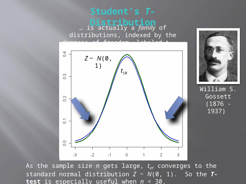
Student’s T-Distribution

William S. Gossett (1876 - 1937)

… is actually a family of distributions, indexed by the degrees of freedom, labeled tdf.

As the sample size n gets large, tdf converges to the standard normal distribution Z ~ N(0, 1). So the T-test is especially useful when n < 30.

t1

t2t3

t10

Z ~ N(0, 1)

Student’s T-Distribution

William S. Gossett (1876 - 1937)

… is actually a family of distributions, indexed by the degrees of freedom, labeled tdf.

As the sample size n gets large, tdf converges to the standard normal distribution Z ~ N(0, 1). So the T-test is especially useful when n < 30.

Z ~ N(0, 1)

t4

.025

1.96

Lecture Notes Appendix…

or…

qt(.025, 4, lower.tail = F)[1] 2.776445

Student’s T-Distribution

William S. Gossett (1876 - 1937)

… is actually a family of distributions, indexed by the degrees of freedom, labeled tdf.

Because any t-distribution has heavier tails than the Z-distribution, it follows that for the same right-tailed area value, t-score > z-score.

Z ~ N(0, 1)

t4

.025

.025

1.96 2.776

X = Age at first birth ~ N(μ , σ )

• H0: μ = 25.4 yrs Null Hypothesis

• HA: μ ≠ 25.4 yrs Alternative Hypothesis

Given:

Previously… σ = 1.5 yrs, n = 400, statistically significant at = .05

x 25.6 yrs

Example: n = 16, s = 1.22 yrsx 25.9 yrs,

Now suppose that σ is unknown, and n < 30.

• standard error (estimate) = 1.22 yrs

160.305 yrs

s

n

• .025 critical value = t15, .025

Lecture Notes Appendix…

p-value = 2 ( )P X 25.9

X = Age at first birth ~ N(μ , σ )

• H0: μ = 25.4 yrs Null Hypothesis

• HA: μ ≠ 25.4 yrs Alternative Hypothesis

Given:

Previously… σ = 1.5 yrs, n = 400, statistically significant at = .05

x 25.6 yrs

Example: n = 16, s = 1.22 yrsx 25.9 yrs,

Now suppose that σ is unknown, and n < 30.

• standard error (estimate) = 1.22 yrs

160.305 yrs

95% Confidence Interval =

s

n

• .025 critical value = t15, .025

95% margin of error

= (2.131)(0.305 yrs)

= 0.65 yrs

(25.9 – 0.65, 25.9 + 0.65) =(25.25, 26.55) yrs

Test Statistic:

15

25.9 - 25.4

0.305T

152 ( )P T 1.639

= 2.131

Lecture Notes Appendix…

X = Age at first birth ~ N(μ , σ )

• H0: μ = 25.4 yrs Null Hypothesis

• HA: μ ≠ 25.4 yrs Alternative Hypothesis

Given:

Example: n = 16, s = 1.22 yrsx 25.9 yrs,

Now suppose that σ is unknown, and n < 30.

• standard error (estimate) = 1.22 yrs

160.305 yrs

95% Confidence Interval =

s

n

• .025 critical value = t15, .025 = 2.131

95% margin of error

= (2.131)(0.305 yrs)

= 0.65 yrs

p-value =

152 ( )P T 1.639

= 2 (between .05 and .10)

The 95% CI does contain the null value μ = 25.4. The p-value is between .10 and .20, i.e., > .05. (Note: The R command 2 * pt(1.639, 15, lower.tail = F)

gives the exact p-value as .122.)

Not statistically significant; small n gives low power!= between .10 and .20.

CONCLUSIONS:

Previously… σ = 1.5 yrs, n = 400, statistically significant at = .05

x 25.6 yrs

(25.9 – 0.65, 25.9 + 0.65) =(25.25, 26.55) yrs

2 ( )P X 25.9

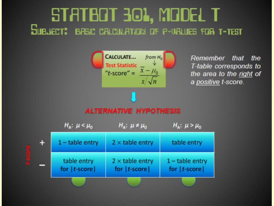
Assuming X ~ N(, σ), test H0: = 0 vs. HA: ≠ 0, at level α…

Lecture Notes Appendix A3.3… (click for details on this section)

If the population variance 2 is known, then use it with the Z-distribution, for any n.

If the population variance 2 is unknown, then estimate it by the sample variance s 2, and use:

• either T-distribution (more accurate), or the Z-distribution (easier), if n 30,• T-distribution only, if n < 30.

To summarize… Assuming X ~ N(, σ)

ALSO SEE PAGE 6.1-28

Assuming X ~ N(, σ), test H0: = 0 vs. HA: ≠ 0, at level α…

If the population variance 2 is known, then use it with the Z-distribution, for any n.

If the population variance 2 is unknown, then estimate it by the sample variance s 2, and use:

• either T-distribution (more accurate), or the Z-distribution (easier), if n 30,• T-distribution only, if n < 30.

To summarize…

Lecture Notes Appendix A3.3… (click for details on this section)

Assuming X ~ N(, σ)

ALSO SEE PAGE 6.1-28

Assuming X ~ N(, σ)

And what do we do if it’s not, or we can’t tell?

Z ~ N(0, 1)

1 2 3 24{ , , ,…, }x x x x

IF our data approximates a bell curve, then its quantiles should “line up” with those of N(0, 1).

How do we check that this assumption is reasonable, when all we have is a sample?

Z ~ N(0, 1)

Assuming X ~ N(, σ)How do we check that this assumption is reasonable, when all we have is a sample?

And what do we do if it’s not, or we can’t tell?

IF our data approximates a bell curve, then its quantiles should “line up” with those of N(0, 1).

Sam

ple

quan

tiles

1 2 3 24{ , , ,…, }x x x x

• Q-Q plot

• Normal scores plot

• Normal probability plot

Assuming X ~ N(, σ)How do we check that this assumption is reasonable, when all we have is a sample?

And what do we do if it’s not, or we can’t tell?

IF our data approximates a bell curve, then its quantiles should “line up” with those of N(0, 1).

• Q-Q plot

• Normal scores plot

• Normal probability plot

(R uses a slight variation to generate quantiles…)

qqnorm(mysample)

Assuming X ~ N(, σ)How do we check that this assumption is reasonable, when all we have is a sample?

IF our data approximates a bell curve, then its quantiles should “line up” with those of N(0, 1).

qqnorm(mysample)

(R uses a slight variation to generate quantiles…)

• Q-Q plot

• Normal scores plot

• Normal probability plot

Formal statistical tests exist; see notes.

And what do we do if it’s not, or we can’t tell?

x = rchisq(1000, 15)hist(x)

y = log(x)hist(y)

Assuming X ~ N(, σ)How do we check that this assumption is reasonable, when all we have is a sample?

And what do we do if it’s not, or we can’t tell?

Use a mathematical “transformation” of the data (e.g., log, square root,…).

X is said to be “log-normal.”

Use a mathematical “transformation” of the data (e.g., log, square root,…).

Assuming X ~ N(, σ)How do we check that this assumption is reasonable, when all we have is a sample?

And what do we do if it’s not, or we can’t tell?

qqnorm(x, pch = 19, cex = .5)qqline(x)

qqnorm(y, pch = 19, cex = .5)qqline(y)

Assuming X ~ N(, σ)How do we check that this assumption is reasonable, when all we have is a sample?

And what do we do if it’s not, or we can’t tell?

Use a mathematical “transformation” of the data (e.g., log, square root,…).

Use a “nonparametric test” (e.g., Sign Test, Wilcoxon Signed Rank Test).

• These tests make no assumptions on the underlying population distribution!

= Mann-Whitney Test

• Based on “ranks” of the ordered data; tedious by hand…

• Has less power than Z-test or T-test (when appropriate)… but not bad.

• In R, see ?wilcox.test for details….

SEE LECTURE NOTES, PAGE 6.1-28 FOR FLOWCHART OF METHODS

See…http://pages.stat.wisc.edu/~ifischer/Intro_Stat/Lecture_Notes/6_-_Statistical_Inference/HYPOTHESIS_TESTING_SUMMARY.pdf