No. 12-9

Potential Effects of the Great Recession

on the U.S. Labor Market

William T. Dickens and Robert K. Triest

Abstract: The effect of the Great Recession on the U.S. labor market will likely persist even after economic output has recovered. Although the recession did not greatly change the relative probabilities of job loss for different types of workers, the long-run impact will vary by worker characteristics. Workers who lost long-term jobs during the Great Recession are at increased risk of future job loss due to the loss of protection afforded by long-term job tenure, and older displaced workers are at a relatively high risk of prolonged spells of unemployment and premature retirement. The recent increase in the job vacancy rate with relatively little change in the unemployment rate suggests a decrease in the efficiency of job matching and an increase in the NAIRU. However, this phenomenon may pass once aggregate demand has increased enough to bring vacancy rates back within their normal range and extended unemployment insurance programs have expired. JEL Classifications: E24, J6, J63, J64 William T. Dickens is a University Distinguished Professor in the department of economics at Northeastern University, a nonresident senior fellow at the Brookings Institution, and a visiting scholar in the research department at the Federal Reserve Bank of Boston. His e-mail address is w.dickens@neu.edu. Robert K. Triest is a vice president and economist in the research department at the Federal Reserve Bank of Boston. His e-mail address is robert.triest@bos.frb.org. The authors thank Gary Burtless and Bart Hobijn, who provided valuable comments. They thank Jamie Fogel for helpful comments and for outstanding assistance with the SIPP data analysis. Thanks also to Tess Forsell, Matthew Jordan, Marie Lekkas, Elizabeth Meyer, Shaun O’Brian, and Irena Tsvetkova for their help in preparing this paper. This paper was written for the Federal Reserve Bank of Boston’s October 2011 conference, “Long-Term Effects of the Great Recession.” The revised papers, discussant comments, panelist remarks, and conference addresses by Ben S. Bernanke, Chairman of the Board of Governors of the Federal Reserve System, and Eric S. Rosengren, President and CEO of the Federal Reserve Bank of Boston, will be published in a special symposium issue of the B.E. Journal of Macroeconomics. This paper presents preliminary analysis and results intended to stimulate discussion and critical comment. The views expressed herein are those of the authors and do not indicate concurrence by the Federal Reserve Bank of Boston, or by the principals of the Board of Governors, or the Federal Reserve System.

This paper, which may be revised, is available on the web site of the Federal Reserve Bank of Boston at http://www.bostonfed.org /economic/wp/index.htm. This version: September 12, 2012

1 Introduction

Previous recessions in the United States have not left many long-lastingscars. Wage movements over past business cycles are hard to detect, la-bor force participation rates quickly return to trend levels, and unem-ployment rates show no long term effects after typically quick recoveries.Other countries have not been as fortunate. At least since Blanchard andSummers (1986) it has been noted that after economic downturns manyother OECD countries have experienced long drops in labor market par-ticipation and persistent high unemployment.

It has been suggested that U.S. exceptionalism in this regard is dueto our experiencing quick recoveries in output after our recessions (see,for example, Ball (1999)). Indeed, none of our postwar recessions havebeen particularly protracted until now. Will this difference, or any otheraspect of the Great Recession, cause medium- or long-term changes in thefunctioning of the U.S. labor market?

We focus on a few areas where previous research and recent dis-cussions have suggested that there may be medium- to long-term labormarket effects. One area where the Great Recession may have a substan-tial impact is on the wages and earnings of workers displaced duringthe recession. Individuals who have been displaced from long-term jobsmay lose the value of job-specific skills, and need to search anew for anemployment situation to which they are well matched. As a result, suchworkers may suffer persistent decreases in labor market earnings. Dis-placement may also have persistent effects on the probabilities of futurejob separations and on the aggregate job finding rate. Workers who gainnew employment after having been displaced from long-term jobs maybe at a higher risk of termination in their new jobs than they were intheir former long-term jobs. Workers separated from long-term jobs mayalso have relatively low job finding rates after displacement due to thegreater specificity of their human capital. The potential for increased la-

1

bor market churning and relatively slow matching of displaced workerswith new job opportunities might contribute to an outward shift of theBeveridge curve and an increase in the non-accelerating inflation rate ofunemployment (NAIRU). We evaluate the evidence for this possibility,and examine the degree to which the apparent outward shift of the Bev-eridge curve may reflect structural issues in the U.S. labor market thatwill persist over a reasonably long horizon.

2 Related Research

A large increase in the fraction of those who are experiencing very longunemployment spells in the wake of the Great Recession has promptedconcern that the pool of unemployed job searchers may, on average, bemore difficult to match to job openings than has been true at the end ofpast recessions. Nearly all studies of the rate of new job finding showthese match rates falling as the duration of unemployment increases.1

Two processes could cause this result. One, it could be that extendedunemployment makes it difficult for people to find jobs or two, it couldbe that those who have trouble finding jobs are disproportionately rep-resented among the ranks of the long-term unemployed. A number ofstudies have attempted to determine the relative importance of these twoexplanations for the downward trend in new job finding rates for thelong-term unemployed. Most studies, using a number of different meth-ods to control for individual differences, still find a substantial downwardtrend in new job finding rates (Lynch, 1985; Arulampalam, Booth, andTaylor, 2000; Imbens and Lynch, 2006). However, all three of these studiesrely on restrictive assumptions about the distribution of individual dif-ferences, leaving the findings suspect. Perhaps more important, the rate

1An exception is that studies often show an increase in the rate of exit from unem-ployment around the time that unemployment benefits expire.

2

of job finding at all durations of unemployment increases considerablywhen labor demand is stronger (Imbens and Lynch, 2006) and it could bethat such increases cancel out the effects of longer average durations ofunemployment.

A related literature examines the effect of unemployment spells onfuture income and the probability of future employment. Again, there isthe problem of separating out individual differences from causal effects.Most typically this is done by comparing an individual’s experience be-fore and after a spell of unemployment. These studies often find that un-employment spells are followed by a medium- to long-term reduction inwages (Addison and Portugal, 1989; Arulampalam, 2001; Corcoran, 1982;Farber, 2005; Gregg and Tominey, 2005; Gregory and Jukes, 2001; Jacob-son, LaLonde, and Sullivan, 1993; Kletzer, 1991; Kletzer and Fairlie, 2003;Podgursky and Swaim, 1987). In a recent paper using U.S. Social Secu-rity records, Von Wachter, Song, and Machester (2009) find that workerswho were displaced from stable jobs during the 1982 recession sufferedearnings losses of approximately 20 percent even after 15 to 20 years.Davis and von Wachter (2011) show that earnings losses attributable todisplacement are roughly twice as large for workers who lose jobs duringa recession compared to those who lose their jobs during an economicexpansion. Farber (2011) documents that the Great Recession has beenaccompanied by job losers experiencing substantial earnings reductions,although he notes that it is not yet clear how prolonged the effects willbe.

Research suggests that the earnings of young workers are particu-larly vulnerable to the effects of recessions. Oreopoulos, von Wachter,and Heisz (2006) find that graduating from college during a recessionresults in earnings losses lasting ten years. However, Von Wachter andBender (2006) show that young German workers who leave apprentice-ship programs during a recession generally suffer less persistent earnings

3

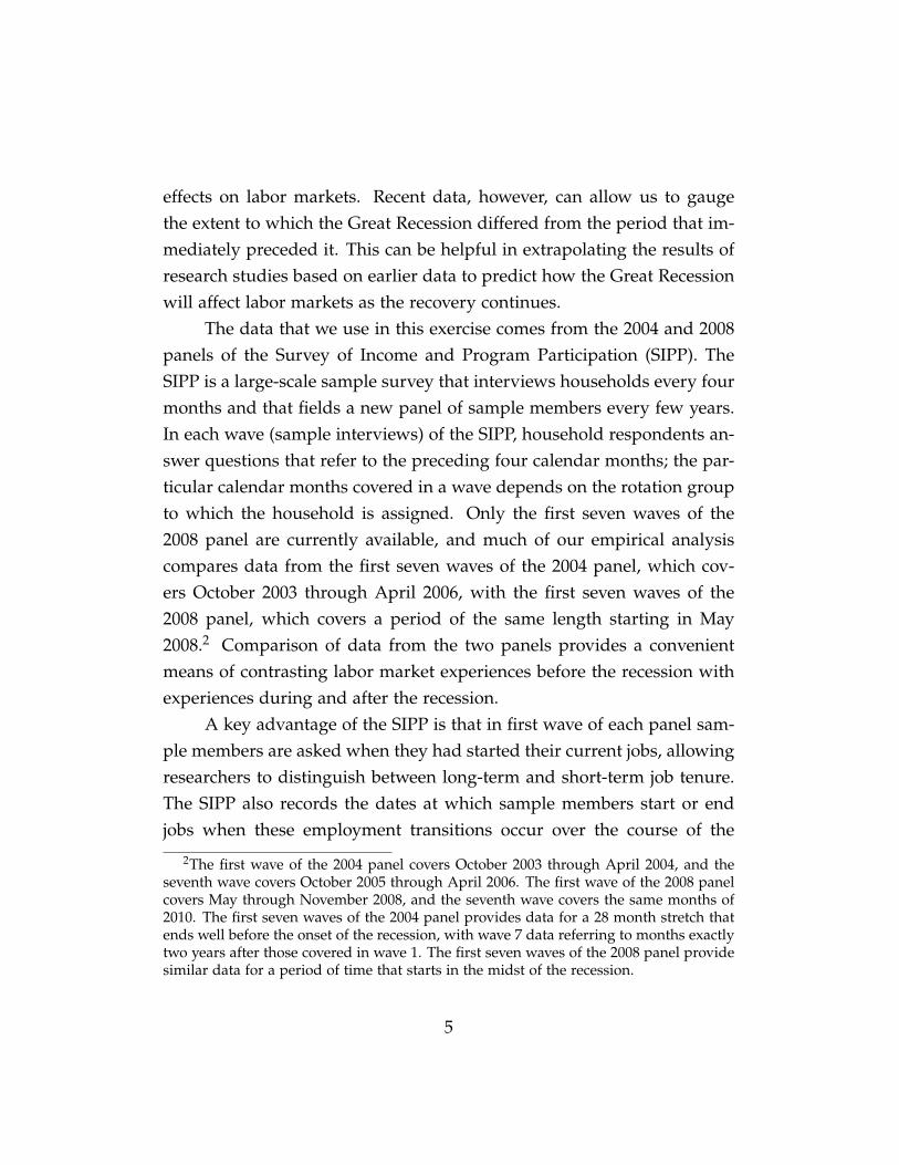
losses.The future employment and earnings of older workers appears to

be sensitive to economic conditions and job displacement. Von Wachter(2007) finds that both economic conditions and job displacement affect theearnings and employment of older men. Sass and Webb (2010) show thatexperiencing a job loss in one’s early 50s is associated with subsequentfuture job losses and unemployment spells. Johnson and Mommaerts(2011) document that although long job tenure reduces the probability ofjob loss, age alone offers no protection. Older workers have slower ratesof reemployment than do younger workers, and suffer much larger re-ductions in earnings upon reemployment. Bosworth and Burtless (2010)note that while decreased labor demand works toward reducing the em-ployment of older workers during a downturn, falling asset prices maylead to increased labor supply through a wealth effect. They find thathigh unemployment is associated with increased claiming rates for SocialSecurity benefits. While Bosworth and Burtless also find that low assetreturns work in the opposite direction, the magnitude of this wealth effectis very small.

A few studies suggest that long spells of unemployment result ina lower probability of future employment for broader groups of workers(Arulampalam, Booth, and Taylor, 2000; Lynch, 1985; Ruhm, 1991), butexcept for Ruhm papers finding this result analyzed British data. Otherstudies of U.S. data conclude that unemployment leaves no long-lastingscars (Corcoran and Hill, 1985; Ellwood, 1982; Genda, Kondo, and Ohta,2010; Heckman and Borjas, 1980)

3 Evidence from the Great Recession

With the U.S. unemployment rate still hovering near 9 percent (as of Oc-tober 2011), it is too soon to fully assess the Great Recession’s long- term

4

effects on labor markets. Recent data, however, can allow us to gaugethe extent to which the Great Recession differed from the period that im-mediately preceded it. This can be helpful in extrapolating the results ofresearch studies based on earlier data to predict how the Great Recessionwill affect labor markets as the recovery continues.

The data that we use in this exercise comes from the 2004 and 2008panels of the Survey of Income and Program Participation (SIPP). TheSIPP is a large-scale sample survey that interviews households every fourmonths and that fields a new panel of sample members every few years.In each wave (sample interviews) of the SIPP, household respondents an-swer questions that refer to the preceding four calendar months; the par-ticular calendar months covered in a wave depends on the rotation groupto which the household is assigned. Only the first seven waves of the2008 panel are currently available, and much of our empirical analysiscompares data from the first seven waves of the 2004 panel, which cov-ers October 2003 through April 2006, with the first seven waves of the2008 panel, which covers a period of the same length starting in May2008.2 Comparison of data from the two panels provides a convenientmeans of contrasting labor market experiences before the recession withexperiences during and after the recession.

A key advantage of the SIPP is that in first wave of each panel sam-ple members are asked when they had started their current jobs, allowingresearchers to distinguish between long-term and short-term job tenure.The SIPP also records the dates at which sample members start or endjobs when these employment transitions occur over the course of the

2The first wave of the 2004 panel covers October 2003 through April 2004, and theseventh wave covers October 2005 through April 2006. The first wave of the 2008 panelcovers May through November 2008, and the seventh wave covers the same months of2010. The first seven waves of the 2004 panel provides data for a 28 month stretch thatends well before the onset of the recession, with wave 7 data referring to months exactlytwo years after those covered in wave 1. The first seven waves of the 2008 panel providesimilar data for a period of time that starts in the midst of the recession.

5

panel.

4 Job Transitions

Table 1 compares the experiences of workers who were employed dur-ing wave 1 of each of the two panels.3 Corroborating patterns found inother data, a much higher proportion of workers observed at the start ofthe 2008 panel left their job involuntarily (through layoff or termination)than did workers observed at the start of the 2004 panel. The 2008 panelmembers were less likely to leave their wave 1 jobs voluntarily (quits)than were the 2004 panel members; they were also less likely to stay attheir initial jobs over the first seven waves of the panel than were the 2004panel members.

The composition of the job losers is important for assessing the long-term effects of job displacement. If a worker leaves a long-term job, theremay be a substantial loss of job-specific human capital. In contrast, aworker who has been on the job a relatively short time has had littleopportunity to build up capital specific to that job. Workers who havesubstantial job tenure are also likely to be in a situation where both theemployee and the employer view the worker to be well-matched to thejob. If this were not the case, either party would have terminated theemployment relationship before substantial time had passed. Long-termworkers who are displaced from jobs lose their ”match capital” and mustagain search for an employment situation that is a good match for theirskills.

We investigate the composition of job losers in a multinomial logitanalysis of job transitions, the results of which are reported in table 2.All workers who were employed in wave 1 are included in the analysis.Workers are classified in terms of how and whether they left their wave 1

3Workers holding more than one job in wave 1 were excluded from these calculations.

6

jobs by the end of the wave 7 reference period: workers may have stayedin their initial job, left that job involuntarily, or left that job voluntarily. Wetreat staying at the initial job as the base case, and report the multinomiallogit results for the probability of involuntary or voluntary transitionsrelative to staying at the initial job. The analysis is purely descriptive,and is not intended to capture the parameters of an underlying structuralmodel of employment transitions.

The coefficients on the conditioning variables are generally of theexpected signs and magnitudes. Coefficients on dummy variables for jobtenure indicate that the probability of either a voluntary or involuntaryjob transition decreases sharply with time for the first few years of em-ployment. In contrast, the probability of an involuntary transition variesrelatively little with age. Young (under 25 years of age) and old (over 59years of age) workers are at significantly higher risk of involuntary tran-sition than those in the intermediate age groups, but the magnitudes ofthe effects for age are much smaller than those for job tenure. The ageeffects are larger for voluntary transitions than they are for involuntarytransitions, most likely due to young workers leaving jobs for school-ing or changing jobs, and older workers leaving jobs for retirement. Theprobability of an involuntary job transition decreases sharply with educa-tional attainment; this is also true for voluntary transitions, but to a lesserextent.

The effect of the Great Recession is measured by an indicator vari-able for membership in the 2008 panel (the omitted group is the 2004panel). The 2008 panel indicator enters the specification as both a maineffect and an interaction with all of the conditioning variables. The main2008 panel effect is large for involuntary transitions, although it is smallerand less statistically significant for voluntary transitions. Although mostof the interaction coefficients are not individually significant, a Wald testdecisively rejects the hypothesis that the group of interaction coefficients

7

are all zero.One interpretation of these results is that the Great Recession greatly

increased the probability of involuntary job transitions across the board,but did not greatly change the relative transition probabilities of differenttypes of workers. Young, less educated, and short-tenured workers wereat a greater risk of displacement both before and during the recession.Very low tenure workers were at somewhat less of a relative disadvan-tage during the recession than before the recession, but this may reflectemployers who adopt a last hired-first fired policy needing to reach fur-ther into the tenure distribution when layoffs increased during the GreatRecession.

Although the Great Recession did not greatly affect the relative risksof job displacement, this does not imply that the overall increased riskof displacement will not have long-term consequences. Although long-tenure workers were not disproportionately displaced during the reces-sion, they were still at increased risk relative to the pre-recession period.To the extent that the displacement of long-tenure workers results in long-term consequences for these workers, the Great Recession will have along-term impact through the increase in the number of long-tenure jobmatches that were destroyed.

5 Earnings Changes

Table 3 displays the mean change in nominal log monthly labor earningsbetween wave 1 and wave 7 for members of the 2004 and 2008 panels whoheld jobs during both of these survey periods. The results are separatedfor those who stayed in their wave 1 job, those who voluntarily left theirwave 1 job, and those who involuntarily lost their wave 1 job. In inter-preting this table, it is important to remember that the monthly earningschanges can only be calculated for those job changers who found new

8

jobs by wave 7. Mean earnings growth was lower in the 2008 panel thanin the pre-recession panel for all three groups. Those whose job transi-tions were involuntary fared the worst both before and during the GreatRecession. Nominal monthly earnings increased about 0.1 percent forthe involuntary job changers over the first 7 waves of the 2004 panel, butfell about 8 percent in the 2008 panel. Voluntary job changers had thelargest monthly earnings increase in the pre-recession panel, but in the2008 panel were second to the job stayers. It is evident that job separationsduring the latest recession are having an impact on the monthly earningsof those workers who are observed in new jobs in wave 7, although it isnot clear how long lasting the effect will be.

Table 4 shows results from regressions of the change in log monthlyearnings between wave 1 and wave 7 on the change in log weekly hoursbetween waves 1 and 7, worker characteristics, and an indicator variablefor the 2008 panel. The regressions were estimated separately for jobstayers, those making involuntary transitions, and those making volun-tary transitions. The estimated values of the constant and 2008 panelcoefficient are essentially providing the same information as that shownin table 3, but conditional on changes in weekly hours and worker char-acteristics. The regression estimates are not adjusted to account for anon-random selection of separated workers into reemployment.

Very few of the worker characteristic coefficients are statistically sig-nificantly discernable from zero. This is somewhat surprising, since onewould expect workers with long tenure in their wave 1 jobs to have ex-perienced a greater loss of earnings than did workers displaced fromshorter-term jobs. Experiments with interacting worker characteristicsand the 2008 panel indicator variable generally also yielded insignificantcoefficients. A Wald test of the joint significance of the full set of inter-actions between worker characteristics and the 2008 panel indicator failsto reject the null hypothesis of no interactions for the job stayer and in-

9

voluntary separation regressions, and fails to reject for p values less than0.04 for the voluntary separation regression.

The estimated coefficient on the dummy variable for the 2008 panelis negative for all three groups, but largest in magnitude for workersmaking voluntary job changes. This result is consistent with the dearthof job openings relative to the number of unemployed individuals duringthe 2008 panel period, and helps to explain why quit rates fell so muchduring the recession.

6 Reemployment of Separated Workers

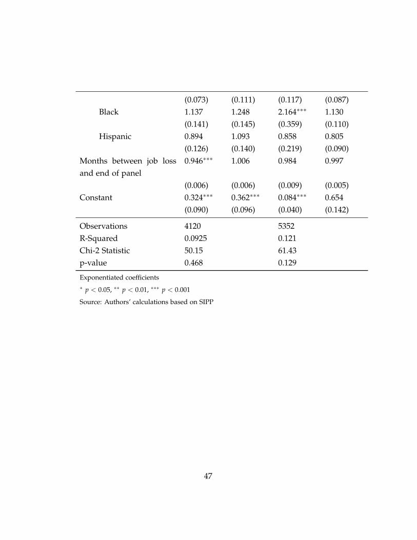
In addition to having an influence on the labor earnings of separatedworkers who regain employment, the Great Recession may also have af-fected labor earnings through influencing the reemployment probabilitiesof workers leaving jobs. Table 5 shows the estimated coefficients frommultinomial logit analysis of the labor force transitions of workers wholeft their wave 1 jobs. The transitions are defined in terms of their wave7 labor force status (employed, unemployed, or not in the labor force).The specification was estimated separately for those who left their wave 1jobs voluntarily and involuntarily. Reemployment is classified as the basecase, and the coefficients have been transformed into relative risk ratios(with statistical significance again measured against the null hypothesisthat the relative risk ratios equal 1).

Not surprisingly, the results indicate that the probability of unem-ployment (relative to reemployment) is much greater in the 2008 panelperiod than in the 2004 panel; this is true both for those losing their jobinvoluntarily as well as for those leaving voluntarily. There is not a sta-tistically significant difference between the two panels in the estimatedprobability of being out of the labor force (relative to reemployment). Forboth the involuntary and voluntary separations, Wald tests fail to reject

10

the hypothesis that the coefficients on the worker characteristic variablesare the same in the two panel periods, so we report only the coefficientsfor the 2004 and 2008 samples combined.

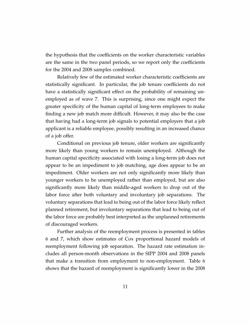
Relatively few of the estimated worker characteristic coefficients arestatistically significant. In particular, the job tenure coefficients do nothave a statistically significant effect on the probability of remaining un-employed as of wave 7. This is surprising, since one might expect thegreater specificity of the human capital of long-term employees to makefinding a new job match more difficult. However, it may also be the casethat having had a long-term job signals to potential employers that a jobapplicant is a reliable employee, possibly resulting in an increased chanceof a job offer.

Conditional on previous job tenure, older workers are significantlymore likely than young workers to remain unemployed. Although thehuman capital specificity associated with losing a long-term job does notappear to be an impediment to job matching, age does appear to be animpediment. Older workers are not only significantly more likely thanyounger workers to be unemployed rather than employed, but are alsosignificantly more likely than middle-aged workers to drop out of thelabor force after both voluntary and involuntary job separations. Thevoluntary separations that lead to being out of the labor force likely reflectplanned retirement, but involuntary separations that lead to being out ofthe labor force are probably best interpreted as the unplanned retirementsof discouraged workers.

Further analysis of the reemployment process is presented in tables6 and 7, which show estimates of Cox proportional hazard models ofreemployment following job separation. The hazard rate estimation in-cludes all person-month observations in the SIPP 2004 and 2008 panelsthat make a transition from employment to non-employment. Table 6shows that the hazard of reemployment is significantly lower in the 2008

11

panel than in the 2004 panel.Table 7 investigates whether the slower rate of job finding during

the Great Recession holds up after controlling for worker characteristics.The panel indicator coefficients are smaller in magnitude (indicating alower hazard rate) than in the earlier table, but are estimated less pre-cisely. A full set of interactions between the 2008 panel indicator andother covariates is included in the analysis, although most of the coeffi-cients on the interactions are close to one and statistically insignificant.Among the main effects, the most notable pattern is that the hazard forreemployment decreases with age starting at about 50 years.

Overall, the empirical results from the reemployment hazards re-inforce the message from table 5: the Great Recession’s main long-runeffect on job finding is likely in its impact on older workers, who tendto have a lower reemployment hazard (relative to younger workers) at allstages of the business cycle. Although older workers are not at a high riskof job loss, once unemployed they tend to stay unemployed longer thando younger workers, and are more likely to permanently leave the laborforce. And once they have lost the protection of a long-term job, they areno longer at lower risk of job loss relative to younger workers.

7 Matching Efficiency and the Beveridge Curve

Although the micro-based evidence on the effects of recessions on sep-aration and job finding rates is not conclusive, aggregate data suggeststhat the Beveridge curve may have shifted out. Figure 1 shows monthlydata for the rate of unemployment and a measure of the vacancy rate con-structed from the Conference Board’s help-wanted index for the periodfrom 1980 through 1983 and annual average data for those same mea-sures from 1965 to 1980. The unemployment rate and the vacancy ratefrom the Job Openings and Labor Turnover Survey (JOLTS) for the pe-

12

riod 2001-2010 is also presented where the JOLTS vacancy rate has beenadjusted to be compatible with the vacancy rate from the help-wantedindex.4 Beveridge curves for the 1980-1987 and the 1954-1969/2001-2009periods are also drawn. In models of frictional unemployment (Blan-chard and Diamond, 1989; 1991) or mismatch unemployment (Shimer,2005), the Beveridge curve is derived as the locus where the number ofjobs being filled is equal to the number of new unemployed workers andthe number of new jobs becoming available. On this curve both the un-employment and vacancy rates remain constant so long as the rate ofnew job creation and the inflow rate of new unemployed workers staysconstant. The position of the Beveridge curve is often interpreted as ameasure of the efficiency of worker-job matching. The further the curveis from the origin the more unemployed workers there are with the samenumber of available job openings. The Beveridge curve relation fits re-markably well for long periods of time. In each of the periods for whichthe curves are drawn, monthly data on vacancies and unemployment re-mained remarkably close to these curves.

Starting in late 2009 the job vacancy rate began to rise while the un-employment rate remained mostly unchanged.5 The last time there wasa sustained increase in the vacancy rate, at similar levels of unemploy-ment, was during the 1970s. That rise coincided with a period duringwhich it is widely believed that the NAIRU increased. Similarly, duringthe late 1980s and 1990s the level of vacancies that coexisted with a partic-ular level of unemployment fell, and this decline coincided with a periodduring which most estimates suggest that the NAIRU fell (Gordon, 1997;Staiger, Stock, and Watson, 1997).

Dickens (2009) developed and estimated a model of the Beveridge

4See Dickens (2009) for an explanation of the method.5In April 2010 there was a large increase in the vacancy rate that should probably be

ignored as it was mainly due to government hiring for the Census. But, even ignoringthat month, there is still a noticeable increase in the vacancy rate over the last year.

13

curve and the Phillips curve that links movement in the Beveridge curveand the position of the long-run Phillips curve or NAIRU. The resultsfrom estimating the model suggest that in the United States all shifts inthe NAIRU result from changes in the efficiency of worker-job matchingas reflected in movements of the Beveridge curve. Using this model wecan determine the implications of the recent increases in the vacancy ratefor the NAIRU.

Figure 2 presents quarterly estimates of the NAIRU from the modelgoing back to 1960. It suggests that since 2009 there has been a notableincrease in the NAIRU from 5 percent to just under 6 percent. Similarly,when we estimate a model allowing for downward nominal wage rigidityto affect the inflation-unemployment tradeoff as in Akerlof, Dickens, andPerry (1996), we find that the lowest sustainable rate of unemploymentrises from 3.9 percent to just over 5 percent. There is some variation whenwe estimate different specifications of these models but all suggest that itwould be possible to lower unemployment by at least 3 percentage pointswithout risking substantial inflation.

While the model interprets the increase in vacancies as indicating anoutward shift in the Beveridge curve, there are several reasons to questionwhether the Beveridge curve really has shifted out. First, the high levelsof unemployment we are now enduring have only been experienced oncebefore during the sample period, 1960 to 2011. During this episode, the1982 recession, the monthly values strayed from the curve that prevailedbefore and after the recession, and in that case the departure suggestedan inward shift in the Beveridge curve. But as time passes this explana-tion seems less and less likely. The departure of the observed vacancyand unemployment rates from proximity to the Beveridge curve in the1982 recession lasted only about one year, while it has been over twoyears since vacancies began increasing in the most recent recession withno similar reduction in unemployment. With adjustments to make the

14

JOLTS vacancy rate equivalent to the one derived from the help-wantedindex, the vacancy rate has recently been below that experienced at anyother time in the sample period. If there is some minimum level of va-cancies that are always present (seasonal jobs that must be filled, firmslooking for highly qualified labor at significantly below market wages)then the Beveridge curve will not have the same shape in the vicinity ofthat minimum. In figure 1 the curve could bend in to the right as thelevel of vacancies approached that minimum, as this would reduce theextent to which the current level of vacancies departs from the 2001-2009Beveridge curve.

Note also that the Beveridge curve is the locus where the unemploy-ment rate and the vacancy rate will settle given a constant rate of new jobcreation and entry of newly unemployed workers to the labor market.During a recession these rates are not constant. When the rate of newjob creation falls, initially the vacancy rate declines faster than the unem-ployment rate increases. During an expansion, the opposite happens asnew job creation causes the vacancy rate to rise before the unemploymentrate begins to fall. These tendencies are exacerbated as frustrated workersleave the labor market when jobs are hard to find (causing the increasein the unemployment rate to lag the decline in vacancies) and enter thelabor market as jobs become easier to find (causing the decline in the un-employment rate to again lag the change in vacancies). This leads to aclockwise movement around the Beveridge curve as it is depicted in fig-ure 1. This lag is barely apparent in the 1980 and 2001 recessions, but ispronounced in the 1982 recession-the only other time in the sample pe-riod that unemployment approached the levels experienced in the mostrecent recession.6

6Tasci and Lindner (2010) have also pointed out the tendency for the unemploymentrate-vacancy rate points to circle the Beveridge curve. They present three previous ex-amples, 1975, 1982 and 2001. As shown in figure 1 the cycle in 2001 was quite muted.The cycle in 1975 took place while the Beveridge curve was moving out. Their use ofquarterly rather than monthly data makes the 2009-2010 move look muted relative to

15

It is possible that the failure of the U.S. unemployment rate to fall inresponse to the increase in vacancies during the last two years is due tothe slow response of the unemployment rate to an increase in the availablejobs. But a direct comparison of what happened recently and in the earlierepisode casts doubt on this explanation. In 1982-1983 it only took twomonths after the vacancy rate began to increase before the unemploymentrate began to decline fairly quickly. It has been over two years since thevacancy rate began to increase following the most recent recession andthe unemployment rate has hardly declined at all. This seems like toolong a lag to be explained by labor market dynamics. We therefore turnto other potential explanations for deterioration in the efficiency of labormarket matching.7

As reviewed earlier, the research on how the duration of unemploy-ment spells affects job finding rates offers some support for the hypoth-esis of hysteresis in unemployment. More direct evidence on Ball’s hy-pothesis comes from a study by Llaudes (2005). For a sample of OECDcountries he estimates Phillips curves, separating out the effect of the un-employment rate for those out of work for more than a year and thoseout of work for less than a year. Llaudes finds that only those individu-als who are unemployed for less than a year put downward pressure onprices while those unemployed for more than a year apparently have noeffect on wages.

We have been able to almost exactly replicate Llaudes’s result in anupdated dataset that we have collected. However, the result is not robustto small changes in the specification. In particular, when the unemploy-ment rate is broken down into as fine a set of durational categories aspossible, only the category for unemployment lasting for 6 to 12 monthsputs statistically significant downward pressure on wages. Further, any

the comparison periods.7Lubik (2011) using a labor market search model rejects the hypothesis of no shift in

the Beveridge curve in the recent period.

16

set of categories that includes the 6 to 12 month duration will be found toput significant downward pressure on wages, while no set of categoriesthat does not contain it is ever statistically significant or has a large neg-ative coefficient. This holds true even if countries whose unemploymentbenefits normally expire after six months are removed from the sample.These results make no sense for the U.S. economy, and little sense forthe rest of the world. A possible explanation for these results is that the6-12 months category is the one that is most highly correlated with theoverall unemployment rate (> 0.9) so it may just be standing in for totalunemployment in the Phillips curve.

Overall, there is not much evidence to support the hypothesis thatextended periods with high rates of long-term unemployment will leadto an increase in the NAIRU in the United States, but this is not to saythat there is strong evidence against the hypothesis either. Given thisconclusion, we turn to the evidence for other possible explanations of thedeterioration in U.S. labor market efficiency.

8 Other Potential Explanations for an Outward

Shift in the Beveridge Curve

Following the rise in the U.S. job vacancy rate, three other explanationsfor the reduction in labor market efficiency have been circulating. First,in response to the increasing numbers of long-term unemployed, the fed-eral government has extended the duration of unemployment benefitsseveral times. There is considerable evidence that increases in the du-ration of unemployment benefits increase unemployment durations andunemployment rates. Second, a mismatch between the skills of the un-employed and those demanded by employers has been offered as anotherexplanation. Finally, it has been suggested that a mismatch between thelocation of available jobs and unemployed workers might help explain

17

the worsening efficiency of labor market matching, and that this problemmight be exacerbated by difficulties in the U.S. housing and mortgagemarkets. These three explanations are examined below in more detail.

8.1 Extended Unemployment Benefits

Several studies have looked at the role that unemployment benefits maybe playing in increasing the unemployment rate by extending the timeunemployed workers are willing to search for jobs. Several of these stud-ies use previous estimates of the effects of benefit duration on unemploy-ment duration to compute the effects of current policy on unemployment(Aaronson, Mazumder, and Schechter, 2010; Elsby, Hobijn, and Sahin,2010). Such studies produce a range of the estimated increase in theunemployment rate from 0.4 to 1.8 percentage points. A problem withthese studies is that the estimates of the impact of extended benefits weremade when the U.S. unemployment rate was much lower and jobs wereeasier to find. It is possible that such estimates overstate the impact inthe current situation. Valletta and Kuang (2010) take a different approachto estimating the impact of extended benefits. They compare the unem-ployment durations of those who are eligible for unemployment benefitsand those who are not as the duration of benefits is extended, and con-clude that extended benefits increase the unemployment rate by about0.8 percentage points. Valletta and Kung’s estimate of the impact of ex-tended benefits is very close to our estimate of the increase in the naturalrate and is slightly below the mid-range of previous estimates. However,Rothstein (2011) analyzes how extended benefits affect the probability ofleaving unemployment using data from after the peak of the Great Reces-sion, and estimates that the benefit extensions raised the unemploymentrate by only 0.2 to 0.6 percentage points. Thus, it seems likely that a sub-stantial part of our estimate of the increase in the NAIRU is due to theeffect of having extended unemployment benefits, but there is uncertainty

18

regarding the precise magnitude. An important implication of the effectof extended benefits on the increase in the NAIRU is that the portion ofthe increase due to extended benefits could be expected to go away asthese benefits are withdrawn with an improving economy.

8.2 Skills Mismatch

It seems likely that in the wake of the Great Recession the U.S. willundergo some structural transformation. The housing boom probablybrought more workers into the construction industry than can be sus-tained in the long run. The financial sector may contract relative to itspre-recession size as well. To the extent that it takes a long time forworkers to move from one type of employment to another, structuralshifts could cause extended increases in the equilibrium level of unem-ployment (Lilien, 1982). The 2001 recession seems to have involved a fairamount of structural reallocation (Groshen and Potter, 2003) and this mayexplain why it took a longer time than usual to bring the unemploymentrate down during the recovery. To what degree is structural mismatchpresent in our economy today and has the degree of mismatch increasedwith the worsening efficiency of the labor market?

Figure 3 presents the ratio of vacancies to unemployment in sev-eral different industries. While it is possible to discern the increase invacancies over recent months in some industries, the ratio remains sub-stantially depressed in all industries. What we do not see is any industrywith high vacancy-unemployment ratios. It is thus hard to make a casefor structural mismatch being a major problem today.

An index of the extent of mismatch between unemployed workersand available jobs can be constructed by subtracting the fraction of un-employed workers in each industry from the fraction of vacant jobs ineach industry and taking its absolute value. This result can be thoughtof as the fraction of workers who would have to move in order for the

19

fraction of workers unemployed in each industry to equal the fractionof all vacancies in that industry.8 Figure 4 shows this measure, our esti-mate of the NAIRU, and the actual unemployment rate from 2001 to date.While the measure of mismatch rose considerably during the early phaseof the recent recession, it has dropped off since then and has returnednow to levels that prevailed during the mid-2000s when unemploymentwas much lower and our estimate of the NAIRU was constant at 5 per-cent. The rise during the early part of the most recent recession need notreflect a temporary rise in structural unemployment. Abraham and Katz(1986) showed that business cycles affect different industries during dif-ferent phases. This can produce the appearance of structural mismatchwhich dissipates as the effects of the recession become widespread.

Although the JOLTS does not contain information on the occupa-tions that created the vacancies, the Conference Board’s Help WantedOnline data do. Researchers at the Federal Reserve Bank of New York(Sahin et al., 2011) have used that data to construct the same sort of mis-match index used here. They find that there has been an increase in themismatch between workers and jobs; the pattern is similar to that seen infigure 4, with a rise beginning in late 2006 and a decline starting in 2009.The timing of these changes suggests that they have nothing to do withthe outward shift in the Beveridge curve. Note that it would be entirelypossible for the mismatch to increase and for it to have no impact onstructural unemployment if the reallocation of workers between differentoccupations was easy at the margin.

8If the matching function exhibits constant returns to scale and the efficiency ofmatching is the same in all cells, an allocation of the unemployed that equates thefraction of vacancies and unemployed in each cell will maximize the match rate andminimize the unemployment rate.

20

8.3 Geographic Mismatch

A similar analysis can be conducted for the extent of geographic mis-match, but the JOLTS data on vacancies are only available at a very highlevel of aggregation-the four large Census regions: Northeast, South,Midwest, and West. Figure 5 presents a graph of the mismatch index byregion from 2001 to date along with the NAIRU estimate and the actualunemployment rate. Not only is there no apparent relationship betweenthe degree of mismatch and our estimate of the NAIRU, but the fractionof workers who would have to relocate to equalize the fraction of unem-ployed and job vacancies in each region declined while the NAIRU wasincreasing. Using the Conference Board’s Help Wanted Online data Sahinet al. (2011) perform a similar exercise at a finer level of disaggregationand reach the same conclusion.

There is some reason to suspect that a combination of geographicmismatch and problems in the housing market could be responsible forthe reduced level of matching efficiency in the U.S. labor market. In aseries of papers Oswald (1996; 1997) has suggested that the level of theNAIRU in a country is closely linked to the fraction of housing that isowner-occupied.9 Oswald argues that high owner-occupancy rates makeit difficult for the unemployed to move when jobs become available else-where. In the past, the United States has been a huge outlier in thisanalysis, having both a high rate of owner-occupied housing and a lowNAIRU. Oswald has explained this discrepancy by pointing to the greaterease of transacting housing sales in the United States and the efficiencyof the U.S. mortgage market. However, with a large fraction of the U.S.housing stock underwater and the recent tightening of credit standardsfor mortgages, it is possible that our high owner-occupancy rates are nowmaking the reallocation of labor substantially more difficult.

9See Havet and Penot (2010) for a skeptical view of the relationship that Oswaldpoints to.

21

There have been many studies of the effects that “housing lock” mayhave on labor market mobility.10 Most studies performed before the re-cent recession found evidence that distress in housing markets reducedlabor mobility. However, more recent studies generally find little evi-dence that long distance moves have been impeded.1112 An exceptionto this is the work by Batini et al. (2010) that argues for a substantialrole for skills mismatch in combination with a depressed housing mar-ket in increasing unemployment, but the paper has a number of seriousflaws. The conclusions are drawn from a regression of the unemploy-ment rate on skill mismatch, housing market distress, and an interactionof the two variables. The first problem is that the index of skill mismatchcompares the educational level of the unemployed workers not to the de-mands of available jobs but to that of the average employed person. Sinceunemployment rates among the least skilled tend to rise most during re-cessions, this would induce a positive correlation between mismatch andunemployment. Second, the correlation between housing market distressand unemployment could be spurious since both could be due to adverseeconomic conditions in the state. Batini et al. recognize this and attemptto ameliorate the problem using the share of subprime mortgages amongall mortgages in the state as an instrument, but this is as likely to becorrelated with economic distress as is the state of the housing market,as families with poor employment prospects may be forced into takingsubprime loans.

While there is little evidence that housing lock is currently causing

10See Chan (2001), Ferreira, Gyourko, and Tracy (2010), Henley (1998), and Quigley(1987; 2002). See Schulhofer-Wohl (2011) for a different view.

11Short distance moves are defined as within county and a reduction in this categorywould be unlikely to affect job matching.

12For example, see Donovan and Schnure (2011), Barnichon and Figura (2010), andMolloy, Smith, and Wozniak (2011). Modestino and Dennett (2012) present evidencesupportive of negative housing equity reducing migration of homeowners, althoughthey find that it has only a negligible effect on the national unemployment rate.

22

structural unemployment, that could be because there are not enoughavailable jobs to make moving worthwhile. However, if the U.S. hous-ing market remains distressed as the economy picks up, it is possiblethat housing market problems could cause future problems for the labormarket.

9 Conclusion

The Great Recession appears to be exerting an influence on the U.S. labormarket that will likely persist even after economic output has recovered.Here we review our main conclusions.

One channel through which job displacement associated with theGreat Recession will likely have a long-term impact is in probabilitiesof future job separations. Although the relative risk of job loss did notincrease for long-term employees during the recent recession, their rate ofjob loss went up along with those of other groups. And once reemployed,they will be at higher risk of future job loss because they will have lost theprotection afforded by long job tenure. One caveat to this conclusion isthat it depends on job tenure being a characteristic of the worker-firm jobmatch, and not just a factor correlated with worker characteristics that aredesirable and observable to employers but unobservable to researchers.

Although involuntary job loss is associated with decreased earningsin the short term, it is puzzling that this effect does not appear to be espe-cially strong for those losing long-term jobs and then starting a new job.It may be the case that those who will eventually experience the greatestearnings loss upon reemployment are not yet observed in new jobs in theSIPP data. Or it may be that the persistent earnings losses of long-termdisplaced workers found in earlier research were specific to characteris-tics of the lost jobs in those studies (for example, rents associated withunionization) that are less prevalent now.

23

For older displaced workers, the relatively low probabilities of reem-ployment and relatively high probabilities of leaving the labor force arecause for concern. Although this group’s overall labor force participationhas been surprisingly high, this number appears to reflect workers whohave not lost their jobs electing to retire at somewhat older ages thanhas been the norm in the recent past. Older displaced workers are atrelatively high risk of prolonged spells of unemployment and prematureretirement. Although job loss during the Great Recession was not dispro-portionately high for older workers relative to younger workers, the rateof job loss rose for older workers along with other groups, resulting in anincrease in the pool of displaced older workers who are at risk.

The recent increase in the vacancy rate, while the unemploymentrate has remained mostly unchanged, probably does suggest a declinein the efficiency of the matching process in the U.S. labor market andan increase in the NAIRU. Estimates from our model of the NAIRU asa function of labor market efficiency suggests that it has increased byabout 1 percentage point. However, this may be a phenomenon that willpass once aggregate demand has increased enough to bring vacancy ratesback within their normal range and extended unemployment insuranceprograms have expired. Our findings are consistent with those of otherresearch, such as Elsby et al. (2011) and Daly et al. (2011), that concludesthat the high unemployment rates experienced in the wake of the GreatRecession are primarily due to insufficient demand rather than due tostructural factors.

Of the explanations for the apparent outward shift of the Beveridgecurve considered here, it seems likely that extended unemployment ben-efits explain some, if not all, of this shift. An improvement in the rateof unemployment will allow the federal government to drop extendedbenefit programs and that should further reduce the unemployment rate-possibly bringing back the levels of unemployment that prevailed before

24

the Great Recession.

References

Aaronson, Daniel, Bhashkar Mazumder, and Shani Schechter. 2010.“What is Behind the Rise in Long-Term Unemployment?” EconomicPerspectives 34(2): 28–51. Available at http://www.chicagofed.

org/digital_assets/publications/economic_perspectives/2010/

2qtr2010_part1_aaronson_mazumder_schechter.pdf.

Abraham, Katherine G., and Lawrence F. Katz. 1986. “Cyclical Unemploy-ment: Sectoral Shifts or Aggregate Disturbances?”.” Journal of PoliticalEconomy 94(3): 507–522.

Addison, John T., and Pedro Portugal. 1989. “Job Displacement, Rela-tive Wage Changes, and Duration of Unemployment.” Journal of LaborEconomics 7(3): 281–302.

Akerlof, George A., William T. Dickens, and George L. Perry. 1996. “TheMacroeconomics of Low Inflation.” Brookings Papers on Economic Activ-ity 1: 1–59. Washington, DC: The Brookings Institution.

Arulampalam, Wiji. 2001. “Is Unemployment Really Scarring? Effectsof Unemployment Experiences on Wages.” Economic Journal 111(475):F585–F606.

Arulampalam, Wiji, Alison L. Booth, and Mark P. Taylor. 2000. “Unem-ployment Persistence.” Oxford Economic Papers 52(1): 24–50.

Ball, Laurence. 1999. “Aggregate Demand and Long-Run Unemploy-ment.” Brookings Papers on Economic Activity 189–236.

Barnichon, Regis, and Andrew Figura. 2010. “What Drives Movement inthe Unemployment Rate? A Decomposition of the Beveridge Curve.”

25

Finance and Economic Discussion Series (48). Available at http://www.

federalreserve.gov/pubs/feds/2010/201048/201048pap.pdf.

Batini, Nicoletta, Oya Celasun, Thomas Dowling, Marcello Estavao, Geof-frey Keim, Martin Sommer, and Evridiki Tosuta. 2010. “United States:Selected Issues Paper.” Washington, DC: International Monetary Fund.

Blanchard, Olivier J., and Peter A. Diamond. 1989. “The BeveridgeCurve.” Brookings Papers on Economic Activity 1: 1–60.

Blanchard, Olivier J., and Peter A. Diamond. 1991. “The AggregateMatching Function.” NBER Working Papers 3175, National Bureau ofEconomic Research.

Blanchard, Olivier J., and Lawrence H. Summers. 1986. NBER Macroeco-nomics Annual, vol. 1, chap. Hysteresis and the European Unemploy-ment Problem, 15–78. Cambridge, MA: The MIT Press.

Bosworth, Barry P., and Gary Burtless. 2010. “Recessions, Wealth De-struction, and the Timing of Retirement.” Center for Retirement Re-search Working Paper 2010-22. Chestnut Hill, MA: Boston College.Available at http://crr.bc.edu/wp-content/uploads/2010/12/wp_

2010-221.pdf.

Chan, Sewin. 2001. “Spatial Lock-in: Do Falling House Prices ConstrainResidential Mobility.” Journal of Urban Economics 49(3): 567–586.

Corcoran, Mary. 1982. The Youth Labor Market Problem: Its Nature, Causes,and Consequences, chap. The Employment and Wage Consequences ofTeenage Women’s Nonemployment, 391–426. Chicago: University ofChicago Press.

Corcoran, Mary, and Martha S. Hill. 1985. “Recurrence of Unemploymentamong Adult Men.” Journal of Human Resources 20(2): 165–183.

26

Daly, Mary, Bart Hobijn, Aysegul Sahin, and Rob Valletta. 2011. “ARising Natural Rate of Unemployment: Transitory or Permanent?”Federal Reserve Bank of San Francisco Working Paper Series: 2011-05. http://www.frbsf.org/publications/economics/papers/2011/

wp11-05bk.pdf.

Davis, Steven J., and Till M. von Wachter. 2011. “Recessions and the Costsof Job Loss.” Working Paper No. 17638. Cambridge, MA: NationalBureau of Economic Research.

Dickens, William T. 2009. Understanding Inflation and the Implications forMonetary Policy: A Phillips Curve Retrospective, chap. A New Method forEstimating Time Variation in the NAIRU, 207–230. Cambridge, MA:The MIT Press.

Donovan, Colleen, and Calvin Schnure. 2011. “Locked In the House:Do Underwater Mortgages Reduce Labor Market Mobility?” http:

//ssrn.com/abstract=1856073.

Ellwood, David T. 1982. The Youth Labor Market Problem: Its Nature, Causes,and Consequences, chap. Teenage Unemployment: Permanent Scars orTemporary Blemishes?, 349–390. Chicago: University of Chicago Press.

Elsby, Michael W. L., Bart Hobijn, and Aysegul Sahin. 2010. “The LaborMarket in the Great Recession.” Brookings Papers on Economic Activity 1:1–48.

Elsby, Michael W. L., Bart Hobijn, Aysegul Sahin, and Robert G. Valletta.2011. “The Labor Market in the Great Recession: An Update.” Work-ing Paper 2011-29. San Francisco: Federal Reserve Bank of San Fran-cisco. Available at http://www.frbsf.org/publications/economics/

papers/2011/wp11-29bk.pdf.

27

Farber, Henry S. 2005. “What Do We Know about Job Lossin the United States? Evidence from the Displaced Work-ers Survey, 1984-2004.” Economic Perspectives 19(2): 13–28. Chicago: Federal Reserve Bank of Chicago. Availableat http://www.chicagofed.org/digital_assets/publications/

economic_perspectives/2005/ep_2qtr2005_part2_farber.pdf.

Farber, Henry S. 2011. “Job Loss in the Great Recession: Historical Per-spective from the Displaced Workers Survey, 1984-2010.” WorkingPaper No. 17040. Cambridge, MA: National Bureau of Economic Re-search.

Ferreira, Fernando, Joseph Gyourko, and Joseph Tracy. 2010. “HousingBusts and Household Mobility.” Journal of Urban Economics 68(1): 34–45.

Genda, Yuji, Ayako Kondo, and Souichi Ohta. 2010. “Long-Term Effectsof a Recession at Labor Market Entry in Japan and the United States.”Journal of Human Resources 45(1): 157–196.

Gordon, Robert J. 1997. “The Time-Varying NAIRU and its Implicationsfor Economic Policy.” Journal of Economic Perspective 11(1): 11–32.

Gregg, Paul, and Emma Tominey. 2005. “The Wage Scar from Male YouthUnemployment.” Labour Economics 12(4): 487–509.

Gregory, Mary, and Robert Jukes. 2001. “Unemployment and SubsequentEarnings: Estimating Scarring among British Men 1984-94.” EconomicJournal 111(475): F607–F625.

Groshen, Erica, and Simon Potter. 2003. “Has Structural Change Con-tributed to a Jobless Recovery?” Current Issues in Economics and Fi-nance 9(8). New York: Federal Reserve Bank of New York. Available athttp://www.ny.frb.org/research/current_issues/ci9-8.pdf.

28

Havet, Nathalie, and Alexis Penot. 2010. “Does Homeownership HarmLabour Market Performances? A Survey.” Groupe d’Analyse et deThorie Economique (GATE) Lyon-St. Etienne. Available at ftp://ftp.

gate.cnrs.fr/RePEc/2010/1012.pdf.

Heckman, James J., and George J. Borjas. 1980. “Does UnemploymentCause Future Unemployment? Definitions, Questions, and Answersfrom a Continuous Time Model of Heterogeneity and State Depen-dence.” Economica 47(187): 247–283.

Henley, Andrew. 1998. “Mobility, Housing Equity, and the Labour Mar-ket.” Economic Journal 108(447): 414–427.

Imbens, Guido W., and Lisa M. Lynch. 2006. “Re-employment Probabili-ties over the Business Cycle.” Portuguese Economic Journal 5(2): 111–134.

Jacobson, Louis S., Robert J. LaLonde, and Daniel G. Sullivan. 1993.“Earnings Losses of Displaced Workers.” American Economic Review83(4): 685–709.

Johnson, Richard W., and Corina Mommaerts. 2011. “Age Differences inJob Displacement, Job Search and Reemployment.” Center for Retire-ment Research at Boston College Working Paper 2011-3. Chestnut Hill,MA: Boston College. Available at http://crr.bc.edu/wp-content/

uploads/2011/01/wp_2011-3.pdf.

Kletzer, Lori G. 1991. Job Displacement: Consequences and Implications forPolicy, chap. Earnings after Job Displacement: Job Tenure, Industry,and Occupation, 107–135. Detroit: Wayne State University Press.

Kletzer, Lori G., and Robert W. Fairlie. 2003. “The Long-Term Costs of JobDisplacement for Young Adult Workers.” Industrial and Labor RelationsReview 56(4): 682–698.

29

Lilien, David M. 1982. “Sectoral Shifts and Cyclical Unemployment.”Journal of Political Economy 90(4): 777–793.

Llaudes, Ricardo. 2005. “The Phillips Curve and Long-Term Unemploy-ment.” Working Paper Series No. 441. Frankfurt: European CentralBank. Available at http://www.ecb.int/pub/pdf/scpwps/ecbwp441.

pdf.

Lubik, Thomas A. 2011. “The Shifting and Twisting Beveridge Curve: AnAggregate Perspective.” Working Paper. Richmond: Federal ReserveBank of Richmond. Federal Reserve Bank of Richmond mimeo (Octo-ber). Available at http://ihome.ust.hk/~yfong/beveridge.pdf.

Lynch, Lisa M. 1985. “State Dependency in Youth Unemployment: A LostGeneration?” Journal of Econometrics 28(1): 71–84.

Modestino, Alicia Sasser, and Julia Dennett. 2012. “Are Americans)Locked into Their Houses? The Impact of Housing Market Condi-tions on State-to-State Migration.” Working Paper 12-1: Boston: Fed-eral Reserve Bank of Boston. Available at http://www.bos.frb.org/

economic/wp/wp2012/wp1201.pdf.

Molloy, Raven Saks, Christopher L. Smith, and Abigail Wozniak. 2011.“Internal Migration in the United States.” Journal of Economic Perspec-tives 25(3): 173–196.

Oreopoulos, Philip, Till von Wachter, and Andrew Heisz. 2006. “TheShort- and Long-Term Career Effects of Graduating in a Recession:Hysteresis and Heterogeneity in the Market for College Graduates.”Working Paper No. 12159. Cambridge, MA: National Bureau of Eco-nomic Research.

Oswald, Andrew J. 1996. “A Conjecture on the Explanation for High Un-employment in the Industrialized Nations: Part I.” The Warwick Eco-

30

nomics Research Paper Series No. 475. Coventry: University of War-wick. Available at http://www2.warwick.ac.uk/fac/soc/economics/

research/workingpapers/publications/1995-1998/twerp_475.pdf.

Oswald, Andrew J. 1997. “Thoughts on NAIRU.” Journal of EconomicPerspectives 11(4): 227–228.

Podgursky, Michael, and Paul Swaim. 1987. “Job Displacement and Earn-ings Loss: Evidence from the Displaced Worker Survey.” Industrial andLabor Relations Review 41(1): 17–29.

Quigley, John M. 1987. “Interest Rate Variations, Mortgage Prepaymentsand Household Mobility.” Review of Economics and Statistics 69(4): 636–643.

Quigley, John M. 2002. “Interest Rate Variations, Mortgage Prepaymentsand Household Mobility.” Real Estate Economics 30(3): 345–364.

Rothstein, Jesse. 2011. “Unemployment Insurance and Job Search in theGreat Recession.” Brookings Papers on Economic Activity 143–210.

Ruhm, Christopher J. 1991. “Are Workers Permanently Scarred by JobDisplacements?” American Economic Review 81(1): 319–324.

Sahin, Ayeseg1, Joseph Song, Giorgio Topa, and Giovanni L. Violante.2011. “Measuring Mismatch in the U.S. Labor Market.” Working Paper.New York: Federal Reserve Bank of New York. Available at http:

//nyfedeconomists.org/topa/USmismatch_v14.pdf.

Sass, Steven A., and Anthony Webb. 2010. “Is the Reduction in OlderWorkers’ Job Tenure a Cause for Concern?” Center for RetirementResearch Working Paper 2010-20. Chestnut Hill, MA: Boston Col-lege. Available at http://crr.bc.edu/wp-content/uploads/2010/12/

wp_2010-201.pdf.

31

Schulhofer-Wohl, Sam. 2011. “Negative Equity Does Not Reduce Home-owner Mobility.” Working Paper No. 16701. Cambridge, MA: NationalBureau of Economic Research.

Shimer, Robert. 2005. “The Cyclical Behavior of Equilibrium Unemploy-ment and Vacancies.” American Economic Rview 95(1): 25–49.

Staiger, Douglas, James H. Stock, and Mark W. Watson. 1997. “TheNAIRU, Unemployment and Monetary Policy.” Journal of Economic Per-spectives 11(1): 33–49.

Tasci, Murat, and John Lindner. 2010. “Has the Beveridge Curve Shifted?”Economic Trends, August 10. Cleveland: Federal Reserve Bank of Cleve-land. Available at http://www.clevelandfed.org/research/trends/

2010/0810/02labmar.cfm.

Valletta, Rob, and Katherine Kuang. 2010. “Extended Unemploymentand UI Benefits.” FSBSF Economic Letter. San Francisco: Federal Re-serve Bank of San Francisco. Available at http://www.frbsf.org/

publications/economics/letter/2010/el2010-12.html.

Von Wachter, Till. 2007. “The Effect of Economic Conditions on the Em-ployment of Workers Nearing Retirement Age.” Center for Retire-ment Research Working Paper 2007-25. Chestnut Hill, MA: Boston Col-lege. Available at http://crr.bc.edu/wp-content/uploads/2007/12/

wp_2007-251.pdf.

Von Wachter, Till, and Stefan Bender. 2006. “In the Right Place at theWrong Time: The Role of Firms and Luck in Young Workers’ Careers.”American Economic Review 96(5): 1679–1705.

Von Wachter, Till, Jae Song, and Joyce Machester. 2009. “Long-Term Earn-ings Losses due to Mass Layoffs During the 1982 Recession: An Anal-ysis Using U.S. Administrative Data from 1974 to 2004.” Dept. of Eco-

32

nomics Working Paper. New York: Columbia University . Available athttp://www.columbia.edu/~vw2112/papers/mass_layoffs_1982.pdf.

Figure 1: Historical Beveridge Curves

Notes: The monthly data run from January 1980 through December 1983 and January2001 to March 2011 and. The annual data runs from 1965 through 1980. After 2000vacancy rates are constructed using the Bureau of Labor Statistics’s Job Openings andLabor Turnover Survey (JOLTS). The two measures are harmonized using a methoddescribed in Dickens (2009).

Sources: Authors’ calculations from unemployment data from the Bureau of LaborStatistics (BLS) and vacancy rates from the Conference Board’s help-wanted series andemployment data from the BLS.

33

Figure 2: NAIRU with 90% Confidence Interval (1960-2011)

Source: Authors’ calculations

34

Figure 3: Vacancy/Unemployment By Industry

Source: Authors’ calculations based on vacancy data from the Department of Labor’sJob Openings and Labor Turnover Survey. Data on unemployment by industry fromanalysis of the Current Population Survey.

35

Figure 4: Industry Mismatch

Sources: Authors’ calculations of the mismatch index and NAIRU. Unemploymentrates from the Bureau of Labor Statistics.

36

Figure 5: Region Mismatch

Sources: Authors’ calculations of the mismatch index and NAIRU computed.Unemployment rates from the Bureau of Labor Statistics.

37

Table 1: Job transitions in the first 28 months of SIPP panels

SIPP PanelReason why left job 2004 Panel 2008 Panel Total

Did not leave 69% 63% 66%Invol. term. 11% 19% 15%Vol. term. 20% 18% 19%

N 26,050 26,391 52,441Source: Authors’ calculations using wave 1 SIPP person weights.

38

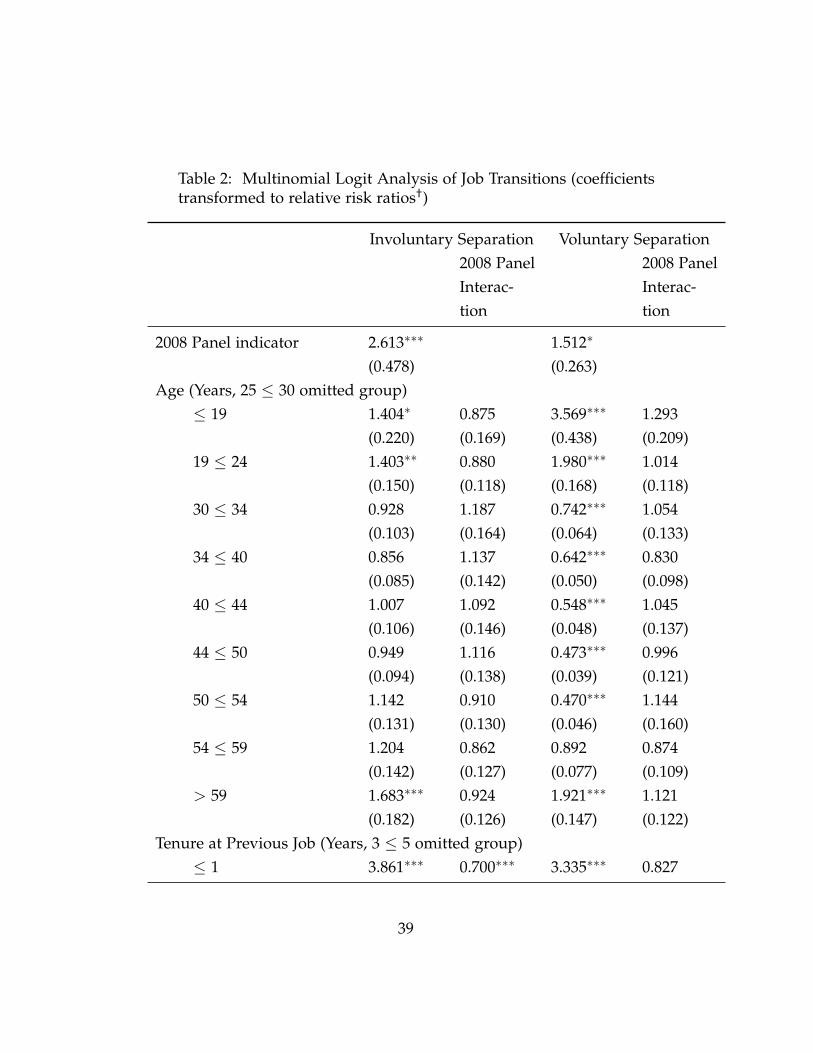
Table 2: Multinomial Logit Analysis of Job Transitions (coefficientstransformed to relative risk ratios†)

Involuntary Separation Voluntary Separation2008 PanelInterac-tion

2008 PanelInterac-tion

2008 Panel indicator 2.613∗∗∗ 1.512∗

(0.478) (0.263)Age (Years, 25 ≤ 30 omitted group)

≤ 19 1.404∗ 0.875 3.569∗∗∗ 1.293(0.220) (0.169) (0.438) (0.209)

19 ≤ 24 1.403∗∗ 0.880 1.980∗∗∗ 1.014(0.150) (0.118) (0.168) (0.118)

30 ≤ 34 0.928 1.187 0.742∗∗∗ 1.054(0.103) (0.164) (0.064) (0.133)

34 ≤ 40 0.856 1.137 0.642∗∗∗ 0.830(0.085) (0.142) (0.050) (0.098)

40 ≤ 44 1.007 1.092 0.548∗∗∗ 1.045(0.106) (0.146) (0.048) (0.137)

44 ≤ 50 0.949 1.116 0.473∗∗∗ 0.996(0.094) (0.138) (0.039) (0.121)

50 ≤ 54 1.142 0.910 0.470∗∗∗ 1.144(0.131) (0.130) (0.046) (0.160)

54 ≤ 59 1.204 0.862 0.892 0.874(0.142) (0.127) (0.077) (0.109)

> 59 1.683∗∗∗ 0.924 1.921∗∗∗ 1.121(0.182) (0.126) (0.147) (0.122)

Tenure at Previous Job (Years, 3 ≤ 5 omitted group)≤ 1 3.861∗∗∗ 0.700∗∗∗ 3.335∗∗∗ 0.827

39

(0.316) (0.073) (0.224) (0.082)1 ≤ 3 1.651∗∗∗ 0.919 1.562∗∗∗ 0.886

(0.148) (0.104) (0.112) (0.094)5 ≤ 9 0.646∗∗∗ 1.093 0.806∗∗ 0.985

(0.070) (0.144) (0.065) (0.116)9 ≤ 14 0.656∗∗∗ 0.866 0.686∗∗∗ 0.876

(0.077) (0.126) (0.062) (0.118)14 ≤ 19 0.504∗∗∗ 0.800 0.617∗∗∗ 1.022

(0.070) (0.143) (0.063) (0.156)> 19 0.373∗∗∗ 1.050 1.067 0.951

(0.050) (0.171) (0.085) (0.112)Highest Education Attained (high school omitted group)

Less than High School 1.245∗∗ 1.299∗∗∗ 1.169 0.940(0.104) (0.090) (0.124) (0.095)

Some post-Secondary 0.882 1.066 0.948 0.940(0.058) (0.057) (0.079) (0.072)

2-Year Degree 0.637∗∗∗ 0.866 0.981 0.907(0.066) (0.068) (0.127) (0.102)

Bachelor’s Degree 0.573∗∗∗ 0.777∗∗∗ 0.847 0.898(0.049) (0.050) (0.089) (0.082)

Master’s or Higher 0.364∗∗∗ 0.813∗∗ 1.005 0.733∗∗

(0.046) (0.063) (0.154) (0.084)U.S. citizen 0.922 1.165 0.825 0.709∗∗

(0.093) (0.104) (0.104) (0.088)Male 0.993 0.681∗∗∗ 1.358∗∗∗ 1.167∗∗

(0.050) (0.027) (0.086) (0.066)Married 0.693∗∗∗ 1.024 1.008 0.882∗

(0.037) (0.045) (0.068) (0.055)Black 1.469∗∗∗ 1.104 0.873 1.152

40

(0.102) (0.067) (0.079) (0.100)Hispanic 1.189∗ 0.975 0.918 0.819

(0.100) (0.072) (0.096) (0.085)Constant 0.127∗∗∗ 0.189∗∗∗

(0.018) (0.023)

Observations 46351R-Squared 0.129Wald Test for Joint Significance of 2008 Panel Interaction TermsChi-squared 136.1p-value 0.000

Exponentiated coefficients∗ p < 0.05, ∗∗ p < 0.01, ∗∗∗ p < 0.001

Source: Authors’ calculations using SIPP† The reported multinomial logit coefficients have been transformed into relative riskratios: each coefficient indicates how a unit increase in the conditioning variable affectsthe probability of the given outcome (voluntary or involuntary transition) relative to thebase case (staying in the job). A value greater than one indicates increased risk of theoutcome relative to the base case, and a value less than one indicates decreased risk; thereported significance levels are for rejection of the null hypothesis that the relative riskratio is equal to one.

Table 3: Mean Change in Nominal Monthly Earnings between Wave 1and Wave 7 (log points)

SIPP PanelReason why left job 2004 Panel 2008 Panel Total

Did not leave 0.081 0.028 0.056Invol. term. 0.006 -0.097 -0.060Vol. term. 0.120 -0.010 0.056Source: Authors’ calculations using wave 1 SIPP person weights.

41

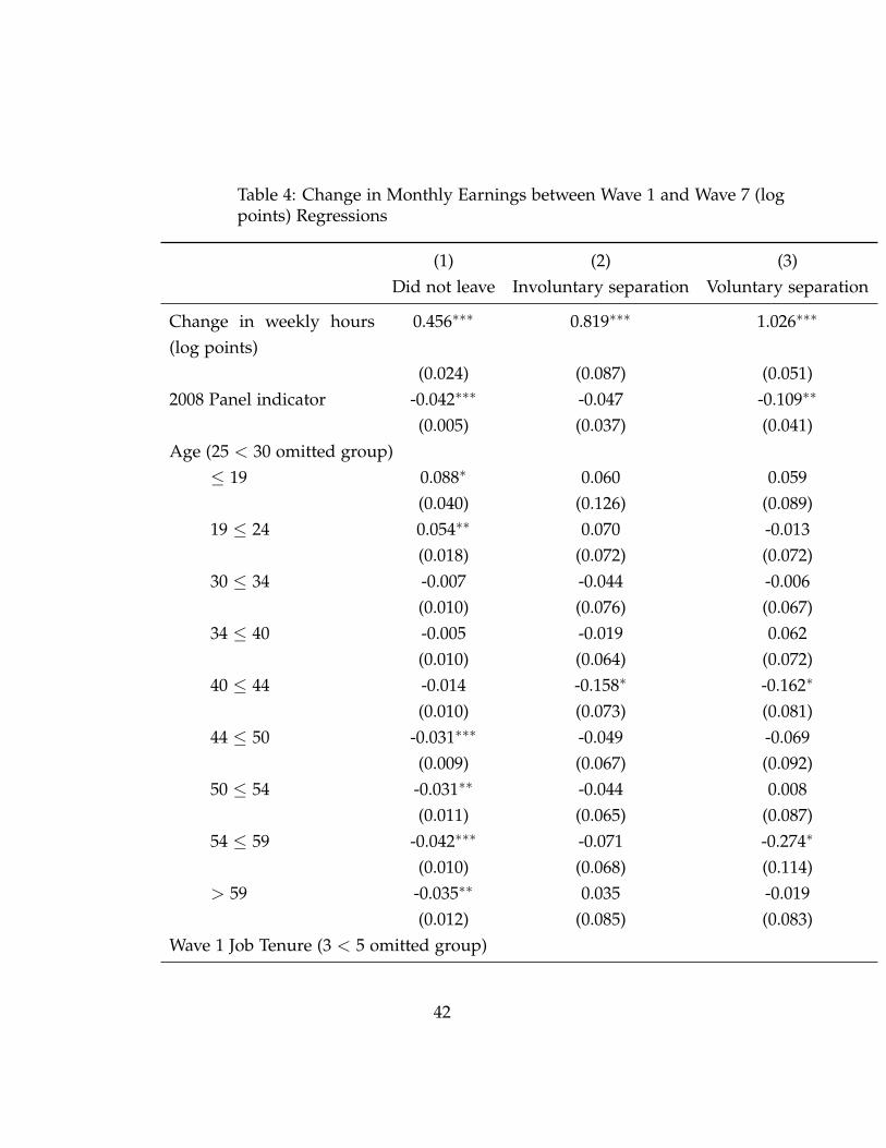
Table 4: Change in Monthly Earnings between Wave 1 and Wave 7 (logpoints) Regressions

(1) (2) (3)Did not leave Involuntary separation Voluntary separation

Change in weekly hours(log points)

0.456∗∗∗ 0.819∗∗∗ 1.026∗∗∗

(0.024) (0.087) (0.051)2008 Panel indicator -0.042∗∗∗ -0.047 -0.109∗∗

(0.005) (0.037) (0.041)Age (25 < 30 omitted group)

≤ 19 0.088∗ 0.060 0.059(0.040) (0.126) (0.089)

19 ≤ 24 0.054∗∗ 0.070 -0.013(0.018) (0.072) (0.072)

30 ≤ 34 -0.007 -0.044 -0.006(0.010) (0.076) (0.067)

34 ≤ 40 -0.005 -0.019 0.062(0.010) (0.064) (0.072)

40 ≤ 44 -0.014 -0.158∗ -0.162∗

(0.010) (0.073) (0.081)44 ≤ 50 -0.031∗∗∗ -0.049 -0.069

(0.009) (0.067) (0.092)50 ≤ 54 -0.031∗∗ -0.044 0.008

(0.011) (0.065) (0.087)54 ≤ 59 -0.042∗∗∗ -0.071 -0.274∗

(0.010) (0.068) (0.114)> 59 -0.035∗∗ 0.035 -0.019

(0.012) (0.085) (0.083)Wave 1 Job Tenure (3 < 5 omitted group)

42

≤ 1 0.035∗∗∗ 0.155∗ 0.012(0.010) (0.061) (0.061)

1 ≤ 3 0.005 0.040 -0.050(0.008) (0.061) (0.064)

5 ≤ 9 -0.012 -0.019 -0.118(0.007) (0.072) (0.080)

9 ≤ 14 -0.017∗ -0.067 -0.181(0.008) (0.078) (0.099)

14 ≤ 19 -0.017 -0.044 -0.453∗∗∗

(0.009) (0.082) (0.134)> 19 -0.010 -0.076 -0.328∗∗

(0.008) (0.087) (0.113)Wave 1 Educational Attainment (high school omitted group)

Less than HighSchool

0.009 -0.016 0.118

(0.011) (0.063) (0.070)Some post-

Secondary-0.005 -0.046 0.153∗∗

(0.006) (0.046) (0.051)2-Year Degree 0.005 0.016 0.118

(0.009) (0.059) (0.082)Bachelor’s Degree 0.009 0.066 0.079

(0.007) (0.057) (0.058)Master’s or Higher 0.009 -0.093 -0.019

(0.008) (0.095) (0.086)U.S. citizen 0.001 0.064 -0.094

(0.011) (0.065) (0.081)Male -0.005 0.052 -0.069

(0.005) (0.036) (0.040)

43

Married -0.001 -0.066 -0.079(0.005) (0.039) (0.044)

Black 0.019∗ -0.071 -0.067(0.008) (0.056) (0.072)

Hispanic -0.014 0.020 -0.062(0.008) (0.048) (0.064)

Constant 0.097∗∗∗ -0.061 0.279∗

(0.015) (0.098) (0.116)

Observations 24938 1399 1384R-SquaredF-Statistic 1.226 0.603 1.557p-value 0.205 0.934 0.0422∗ p < 0.05, ∗∗ p < 0.01, ∗∗∗ p < 0.001

Source: Authors’ calculations based on SIPP

44

Table 5: Multinomial Logit Analysis of Labor Force Status in Wave 7 forJob Changers (coefficients transformed to relative risk ratios)

(1) (2)Base case: Employed inWave 7

Involuntary separation Voluntary separation

unemployed nilf unemployed nilf

2008 Panel indicator 3.518∗∗∗ 0.928 2.523∗∗∗ 1.063(0.368) (0.077) (0.353) (0.066)

Age (25 < 30 omitted group)≤ 19 0.920 2.604∗∗∗ 0.640 1.483∗∗

(0.247) (0.537) (0.203) (0.210)19 ≤ 24 0.995 1.223 0.661 0.858

(0.188) (0.206) (0.189) (0.107)30 ≤ 34 1.246 0.783 0.773 0.765

(0.232) (0.147) (0.260) (0.109)34 ≤ 40 1.136 0.799 1.722∗ 0.957

(0.198) (0.134) (0.456) (0.126)40 ≤ 44 1.351 0.692∗ 1.357 0.572∗∗∗

(0.241) (0.129) (0.397) (0.089)44 ≤ 50 1.616∗∗ 1.001 1.514 0.884

(0.268) (0.165) (0.406) (0.121)50 ≤ 54 1.408 0.964 1.841 1.322

(0.263) (0.182) (0.578) (0.208)54 ≤ 59 2.012∗∗∗ 1.496∗ 2.290∗∗ 2.225∗∗∗

(0.389) (0.281) (0.684) (0.316)> 59 1.757∗∗ 5.035∗∗∗ 1.291 6.184∗∗∗

(0.344) (0.824) (0.422) (0.790)Wave 1 Job Tenure (3 < 5 omitted group)

≤ 1 1.105 1.206 1.183 1.318∗

45

(0.159) (0.168) (0.276) (0.149)1 ≤ 3 0.944 0.886 1.103 1.247

(0.144) (0.133) (0.288) (0.153)5 ≤ 9 1.131 0.924 1.159 1.155

(0.192) (0.161) (0.336) (0.158)9 ≤ 14 1.043 0.761 1.182 1.512∗∗

(0.195) (0.148) (0.406) (0.236)14 ≤ 19 1.288 0.736 1.574 1.857∗∗∗

(0.305) (0.198) (0.590) (0.330)> 19 1.116 1.373 1.588 2.793∗∗∗

(0.233) (0.279) (0.507) (0.414)Wave 1 Educational Attainment (high school omitted group)

Less than HighSchool

1.194 1.220 1.041 1.138

(0.164) (0.152) (0.221) (0.123)Some post-

Secondary0.957 1.039 0.650∗ 0.889

(0.106) (0.111) (0.115) (0.076)2-Year Degree 1.051 0.820 0.587 0.860

(0.172) (0.147) (0.169) (0.117)Bachelor’s Degree 0.790 0.682∗∗ 0.494∗∗ 0.636∗∗∗

(0.108) (0.097) (0.109) (0.067)Master’s or Higher 0.512∗∗ 0.728 0.337∗∗∗ 0.472∗∗∗

(0.115) (0.144) (0.105) (0.060)U.S. citizen 1.172 1.159 0.977 1.088

(0.187) (0.184) (0.308) (0.153)Male 0.923 0.445∗∗∗ 1.113 0.562∗∗∗

(0.078) (0.036) (0.150) (0.036)Married 0.789∗∗ 1.227∗ 0.773 1.209∗∗

46

(0.073) (0.111) (0.117) (0.087)Black 1.137 1.248 2.164∗∗∗ 1.130

(0.141) (0.145) (0.359) (0.110)Hispanic 0.894 1.093 0.858 0.805

(0.126) (0.140) (0.219) (0.090)Months between job lossand end of panel

0.946∗∗∗ 1.006 0.984 0.997

(0.006) (0.006) (0.009) (0.005)Constant 0.324∗∗∗ 0.362∗∗∗ 0.084∗∗∗ 0.654

(0.090) (0.096) (0.040) (0.142)

Observations 4120 5352R-Squared 0.0925 0.121Chi-2 Statistic 50.15 61.43p-value 0.468 0.129

Exponentiated coefficients∗ p < 0.05, ∗∗ p < 0.01, ∗∗∗ p < 0.001

Source: Authors’ calculations based on SIPP

47

Table 6: Cox proportional hazard analysis of re-employment followingseparation

(1) (2)Involuntary separation Voluntary separation

Indicator for 2008 panel 0.819∗∗∗ 0.891∗

(0.035) (0.040)

Observations 70463 103792R-Squared 0.000583 0.000181

Exponentiated coefficients∗ p < 0.05, ∗∗ p < 0.01, ∗∗∗ p < 0.001

48

Table 7: Cox proportional hazard analysis of re-employment followingseparation

(1)Involuntary Separation Voluntary Separation

2008 PanelInterac-tion

2008 PanelInterac-tion

2008 Panel indicator 0.573∗ 0.567(0.147) (0.173)

Age (Years, 25 < 30 omitted group)≤ 19 1.145 1.166 1.596∗∗∗ 0.948

(0.181) (0.250) (0.190) (0.180)19 ≤ 24 1.182 0.995 1.262∗ 1.155

(0.157) (0.174) (0.134) (0.195)30 ≤ 34 0.762 1.202 0.860 1.000

(0.122) (0.242) (0.122) (0.234)34 ≤ 40 0.916 1.029 0.704∗∗ 1.241

(0.129) (0.187) (0.091) (0.274)40 ≤ 44 0.901 1.160 0.788 1.075

(0.124) (0.214) (0.113) (0.279)44 ≤ 50 0.936 0.955 0.814 0.948

(0.122) (0.165) (0.107) (0.218)50 ≤ 54 0.848 1.120 0.568∗∗ 1.437

(0.131) (0.224) (0.101) (0.393)54 ≤ 59 0.670∗ 1.293 0.571∗∗∗ 0.696

(0.113) (0.274) (0.086) (0.198)> 59 0.485∗∗∗ 1.051 0.270∗∗∗ 1.221

(0.076) (0.214) (0.038) (0.279)Wave 1 Job Tenure (Years, 3 < 5 omitted group)

49

≤ 1 0.860 1.131 1.175 1.005(0.098) (0.169) (0.121) (0.176)

1 ≤ 3 1.020 0.899 1.058 1.013(0.122) (0.140) (0.115) (0.189)

5 ≤ 9 1.042 0.797 0.972 0.852(0.150) (0.147) (0.133) (0.201)

9 ≤ 14 0.833 0.942 0.809 1.257(0.148) (0.213) (0.147) (0.376)

14 ≤ 19 0.593∗ 1.971∗ 0.977 0.651(0.149) (0.590) (0.188) (0.258)

> 19 1.023 0.736 0.654∗∗ 0.872(0.203) (0.189) (0.105) (0.245)

Wave 1 Educational Attainment (high school omitted group)Less than High School 0.951 0.768 0.896 0.994

(0.093) (0.105) (0.076) (0.148)Some post-Secondary 1.103 0.967 1.194∗ 1.019

(0.098) (0.112) (0.089) (0.126)2-Year Degree 1.260 0.848 1.067 0.939

(0.184) (0.158) (0.139) (0.204)Bachelor’s Degree 0.989 1.193 1.240∗ 1.295

(0.122) (0.184) (0.123) (0.209)Master’s or Higher 1.410∗ 1.074 1.187 1.729∗

(0.236) (0.227) (0.172) (0.395)U.S. citizen 0.983 1.168 1.053 1.453

(0.133) (0.204) (0.126) (0.309)Male 1.036 1.122 1.179∗∗ 0.948

(0.068) (0.098) (0.068) (0.090)Married 0.874 1.215∗ 0.887 0.991

(0.066) (0.119) (0.062) (0.120)

50

Black 0.790∗ 1.077 0.710∗∗∗ 1.044(0.076) (0.139) (0.063) (0.157)

Hispanic 1.020 1.127 0.715∗∗ 1.289(0.114) (0.160) (0.075) (0.208)

Enrolled in School 0.699∗∗ 0.939 0.663∗∗∗ 0.778(0.084) (0.147) (0.057) (0.103)

Observations 70409 103727R-Squared 0.0059 0.0203

Exponentiated coefficients∗ p < 0.05, ∗∗ p < 0.01, ∗∗∗ p < 0.001

51