The NAIRU, Unemployment and Monetary Policy · The NAIRU, Unemployment and Monetary Policy ......

Journal of Economic Perspectives—Volume 11, Number 1—Winter 1997—Pages 33–49

The NAIRU, Unemployment andMonetary Policy

Douglas Staiger, James H. Stock,and Mark W. Watson

S ince Milton Friedman's (1968) presidential address to the American Eco-nomic Association, one of the most enduring ideas in macroeconomics hasbeen that inflation will increase when unemployment persists below its nat-

ural rate, the so-called NAIRU, or nonaccelerating inflation rate of unemployment.But what is the NAIRU? Is it 5.8 percent as estimated by the CBO (1996)? Is it5.7 percent as used by the Council of Economic Advisors (1996) or 5.6 percent asestimated by Gordon (this issue)? Or can unemployment safely go much lower, asrecently argued by Eisner (1995a,b)? For all of 1995 and the first two quarters of1996, unemployment hovered around 5.6 percent, while inflation remained incheck. This has led to a debate among academics and policymakers over whetherthere has been a decline in the NAIRU and, more generally, whether economistsshould continue to rely on unemployment and the NAIRU as indicators of an over-heated economy (Weiner, 1993, 1994; Tootell, 1994; Fuhrer, 1995; Council of Eco-nomic Advisors, 1996, pp. 51–57; Congressional Budget Office, 1996, pp. 5, 27).

At the heart of this debate lie several empirical questions. Has the NAIRUdeclined in recent years? What is the current value of the NAIRU? How confidentshould economists be in these estimates? How useful is knowledge of NAIRU in

• Douglas Staiger is Assistant Professor of Political Economy, Kennedy School of Government,

Harvard University, Cambridge, Massachusetts. James H. Stock is Professor of Political Econ-

omy, Kennedy School of Government, Harvard University, Cambridge, Massachusetts. Mark

W. Watson is Professor of Economics and Public Affairs, Woodrow Wilson School, Princeton

University, Princeton, New Jersey. Staiger is a Faculty Research Fellow and Stock and Watson

are Research Associates at the National Bureau of Economic Research, Cambridge, Massa-

chusetts. Their e-mail addresses are [email protected], [email protected]

and [email protected], respectively.

34 Journal of Economic Perspectives

anticipating increases in inflation? This paper summarizes recent research and pre-sents some new evidence on these questions.

We begin by discussing and extending recent attempts to estimate the NAIRU.We find that there is statistical evidence that the NAIRU has changed over the past30 years and in particular that the NAIRU has fallen by approximately one per-centage point from its peak in the early 1980s to a current estimate that rangesfrom 5.5 percent to 5.9 percent, depending on the details of the specification.However, the most striking feature of these estimates is their lack of precision. Forexample, the 95 percent confidence interval for the current value of the NAIRUbased on the GDP deflator is 4.3 percent to 7.3 percent. In fact, our 95 percentconfidence intervals for the NAIRU are commonly so wide that the unemploymentrate has only been below them for a few brief periods over the last 20 years.

Faced with this uncertainty about the NAIRU, it is not surprising that forecastsof inflation based on the Phillips curve are insensitive to different assumptionsabout the NAIRU: we find that forecasters using values of the NAIRU ranging from4.5 to 6.5 percent would have produced similar forecasts of inflation over the nextyear. Finally, we find that, although unemployment is a useful predictor of inflationover the next year, other leading indicators of inflation are better, and the relativestrength of other indicators increases at longer forecast horizons. It seems to usthat, in light of this imprecision, the recent debate over whether the NAIRU iscurrently 6 percent or 5.5 percent does little to inform monetary policy.

The NAIRU: Estimates and Confidence Intervals

A Preliminary Look at the DataOne difficulty with empirical examinations of the Phillips curve tradeoff be-

tween inflation and unemployment is the lack of a perfect measure of inflation.The literature on the Phillips curve uses a variety of measures, from broad ones likethe gross domestic product (GDP) deflator to narrow measures of "core inflation,"which is usually defined to exclude prices of food and energy goods. For most ofthis paper, broad inflation will be measured by the percentage growth in the GDPprice index, and core inflation will be measured by the percentage growth in thepersonal consumption expenditure (PCE) price index, excluding expenditures onfood and energy. The results for these two series are typical of those for other broador core price series. The measure of the unemployment rate used throughout isthe civilian unemployment rate for all workers, ages 16 and above.

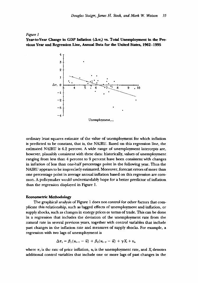
Our main findings are illustrated by the scatterplot in Figure 1. The horizontalaxis shows the unemployment rate in the previous year. The vertical axis shows thechange in the inflation rate from last year to the current year. The data are from1962–1995. There is evidently a negative relationship; for example, inflation in-creased in six of the seven years that unemployment was below 5 percentage points.Also plotted in Figure 1 is the ordinary least squares regression line estimated overthis full sample. The intersection of this line with the unemployment axis is the

Douglas Staiger, James H. Stock, and Mark W. Watson 35

Figure 1Year-to-Year Change in GDP Inflation (Δπ t ) vs. Total Unemployment in the Pre-vious Year and Regression Line, Annual Data for the United States, 1962–1995

ordinary least squares estimate of the value of unemployment for which inflationis predicted to be constant, that is, the NAIRU. Based on this regression line, theestimated NAIRU is 6.2 percent. A wide range of unemployment intercepts are,however, plausibly consistent with these data: historically, values of unemploymentranging from less than 4 percent to 9 percent have been consistent with changesin inflation of less than one-half percentage point in the following year. Thus theNAIRU appears to be imprecisely estimated. Moreover, forecast errors of more thanone percentage point in average annual inflation based on this regression are com-mon. A policymaker would understandably hope for a better predictor of inflationthan the regression displayed in Figure 1.

Econometric MethodologyThe graphical analysis of Figure 1 does not control for other factors that com-

plicate this relationship, such as lagged effects of unemployment and inflation, orsupply shocks, such as changes in energy prices or terms of trade. This can be donein a regression that includes the deviation of the unemployment rate from thenatural rate in several previous years, together with control variables that includepast changes in the inflation rate and measures of supply shocks. For example, aregression with two lags of unemployment is

Δπt = β1(u t – 1 – ū) + β2(ut– 2 – ū) + γXt + vt,

where πt is the rate of price inflation, ut is the unemployment rate, and Xt denotesadditional control variables that include one or more lags of past changes in the


inflation rate and supply shock measures. In this regression, the NAIRU, ū, entersas an unknown parameter.

This version of the model is difficult to estimate because the NAIRU appearstwice and because the model is nonlinear in the parameters. However, these prob-lems are readily handled by rewriting this equation to obtain an equivalent expres-sion that can be estimated by ordinary least squares. After separating out and col-lecting the terms involving the NAIRU, the regression is

where µ = – (β1 + β2)ū. Given ordinary least squares estimates of the constant termµ and coefficients β1 and β2, the NAIRU can be estimated as – µ/(β1 + β2).

The regression line in Figure 1 is a special case of this approach in whichneither ut– 2 nor Xt appear, so that ut– 1 is the only regressor. The ordinary leastsquares regression line in Figure 1 is Δπt = 2.73 – 0.44ut– 1, so the estimated valueof the NAIRU is 2.73/.44 = 6.2 percent. This technique can be extended to as manylags of unemployment as seems appropriate and is the conventional method forthe estimation of the NAIRU as used by Gordon (1982), the Congressional BudgetOffice (1994), Eisner (1995a), Tootell (1994), Weiner (1993, 1994), Fuhrer (1995)and others.1

As mentioned already, this formulation does not allow for time variation in theNAIRU. One approach is to model the natural rate of unemployment as havingdiscrete jumps at certain points in time, an approach used by Gordon (1982), Wei-ner (1993) and Tootell (1994). However, because "break" models of this sort mustbe constrained not to jump too often, these models imply that NAIRU is constantover long periods. For investigating whether the NAIRU has declined in recentyears, we prefer to use a more flexible approach in which the NAIRU is modeledby a flexible polynomial, a so-called "spline."2

Confidence Intervals for the NAIRU

It is impossible to interpret parameters that have been estimated econometri-cally without having a measure of their precision such as their standard errors.However, until recently no such measures of the precision of the NAIRU have beenavailable. Presumably, the reason for this absence is that the NAIRU is a nonlinear

1 Additional recent estimates of the NAIRU or potential GDP appear in Amato (1995); Congressional

Budget Office (1994); Cromb (1993); King, Stock and Watson (1995); Kuttner (1994); Layard, Nickell

and Jackman (1991); Salemi (1996), Setterfield, Gordon and Osberg (1992); Staiger, Stock and Watson

(1996, 1997); and van Norden (1995). Additional recent articles discussing changes in the NAIRU,

stability in the Phillips curve and the implications for monetary policy include Cecchetti (1995); Fair

(1996); Gordon (1990); Juhn, Murphy and Topel (1991); King and Watson (1994); Krugman (1994,

1995, 1996); and Kuttner (1992).2 Specifically, a cubic spline with two knot points is used. Between the knot points, the spline is a third

degree polynomial. These polynomials are constrained to be equal, and to have equal first and second

derivatives, at the knot points. The knot points used are equally spaced values along the time axis; for

the regressions with 138 observations (quarterly, from 1961:III to 1995:IV), the knot points were at

observations 46 and 92.

The NAIRU, Unemployment and Monetary Policy 37

function of regression coefficients (notice that the ß terms appear in the denomi-nator of the expression following the second display equation), and regressionpackages do not automatically produce standard errors for nonlinear functions. InStaiger, Stock and Watson (1997), we used Monte Carlo simulations to comparetwo methods for constructing confidence intervals for the NAIRU, the "delta"method,3 which is a method used by Fuhrer (1995), and an approach that we referto as Fieller's method. Those simulations indicated that intervals constructed usingFieller's method performed significantly better than intervals based on the deltamethod.4 In this article, we therefore focus exclusively on confidence intervals basedon Fieller's method.

Fieller's method is an extension of the technique proposed by E. C. Fieller (1954)to construct a confidence interval for the ratio of the means of two dependent normalrandom variables. A 95 percent confidence interval for, say, a mean can be calculatedby performing hypothesis tests on all possible hypothetical values of the true mean;the set of values not rejected at the 5 percent level constitutes a 95 percent confidenceinterval. To construct a confidence interval for the NAIRU, first select a trial value ofNAIRU, say 6.0, and construct the unemployment gap series, ut – 6.0. If the NAIRUis in fact 6.0, then the true intercept in the regression of Δπt on this unemploymentgap, its lags and the control variables Xt (which include lags of Δπt) is zero, as in thefirst display equation. If the estimated intercept in this regression is statistically insig-nificant at the 5 percent level, then the hypothesis that the NAIRU is 6.0 percent cannotbe rejected at the 5 percent level, that is, an estimated NAIRU of 6.0 percent lies in a95 percent confidence interval. Repeating this for all possible values of the NAIRUproduces the 95 percent confidence interval.

Estimates of the NAIRU and its 95 percent Fieller confidence interval are plot-ted in Figure 2, using data on the quarterly core rate of PCE inflation for 1962–1995. All the specifications reported in this section include four lags of unemploy-ment, four lags of inflation and two supply shock control variables: one to capturethe Nixon wage and price controls, and the other to capture supply shocks to foodand energy prices.5 The NAIRU is estimated to have been higher during the 1970s

5 The delta method is a general technique for constructing asymptotic standard errors for nonlinear

functions of parameters. By using a first-order Taylor series expansion, the nonlinear function is ap-

proximated by a linear function that is asymptotically normally distributed. Standard errors are then

computed using estimated first derivatives. For example, suppose that θ is a vector of parameters, θ is

its estimate, and g(θ) is the function of interest; then the delta method approximates the distribution of

g(θ) by a normal distribution with mean g(θ) and variance ( g/ θ) 'V ( g/dθ), where V is the estimated

variance-covariance matrix of θ and ( g/ θ) is the first derivative of g, evaluated at θ; cf. Greene (1990).4 This is not surprising. The NAIRU is estimated as the ratio of coefficients, and distributions of ratios

of random variables are well known to have nonnormal, even bimodal, distributions. The delta method

approximates the distribution of the estimated NAIRU by a normal, but the Fieller method intervals do

not. An interesting econometric analogy is to instrumental variables estimation. The two-stage least

squares estimator is the ratio of two random variables and, depending on the quality of the instruments,

it can have a bimodal distribution; see for example Charles Nelson and Richard Startz (1990).5 The wage and price control variable, called NIXON, is the sum of the two wage and price control

variables in Gordon (1982); this enters with no lag. The food and energy prices variable, RPFE, is the


Figure 2

Estimate of the NAIRU, 95 percent Confidence Interval and Unemployment, Basedon Core PCE Inflation, 1961:III–1995:IV

and early 1980s than during the 1960s or 1990s; during most of the 1960s, theNAIRU is estimated to have been below 5.5 percent. This variation over time isstatistically significant at the 10 percent level. For these three decades, the 95 per-cent confidence intervals are wide enough to include most observed values of un-employment, with the exception of some cyclical peaks and troughs.

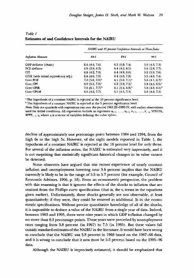
Estimates of the NAIRU are presented in Table 1. In addition to GDP inflationand core PCE inflation, results are reported for other price indexes: the full chain-weighted personal consumption expenditures (PCE) deflator; the all-items con-sumer price index (CPI); the CPIR, which is an adjusted version of the CPI in whichthe CPI for tenants' rent is substituted for the CPI for home ownership between1967–1983; the core CPI and CPIR, which are recalculated to exclude food andenergy; and finally the core CPI-M, which is a weighted median core CPI measure,published by the Federal Reserve Bank of Cleveland. The point estimates of theNAIRU based on these different inflation series are similar. However, there aresubstantial differences in the precision of the estimates. In general, the tightestestimates are found using core inflation, but the particular measure of core infla-tion makes a large difference in the confidence intervals. Even the tightest of theseintervals for 1994:I, based on core CPIR inflation, is 4.8 percent to 6.6 percent,almost 2 percentage points wide.

Past researchers like Weiner (1993) and Tootell (1994) have found evidencethat the NAIRU has changed over the postwar period, and some of the results hereare consistent with this view. The point estimates of the NAIRU in Table 1 show a

log ratio of the wholesale price deflator for food and energy, as defined in King and Watson (1994), tothe CPIR, which is the CPI deflator with a rental cost adjustment as defined in the next paragraph; thisenters with a single lag.


Table 1Estimates of and Confidence Intervals for the NAIRU

decline of approximately one percentage point between 1984 and 1994, from thehigh 6s to the high 5s. However, of the eight models reported in Table 1, thehypothesis of a constant NAIRU is rejected at the 10 percent level for only three.For several of the inflation series, the NAIRU is estimated very imprecisely, and itis not surprising that statistically significant historical changes in its value cannotbe detected.

Some observers have argued that our recent experience of nearly constantinflation and unemployment hovering near 5.6 percent implies that the NAIRUcurrently is likely to be in the range of 5.5 to 5.7 percent (for example, Council ofEconomic Advisors, 1996, p. 53). From an econometric perspective, the problemwith this reasoning is that it ignores the effects of the shocks to inflation that areomitted from the Phillips curve specification (that is, the vt terms in the equationsgiven earlier). Unfortunately, these shocks generally are not observable, at leastquantitatively; if they were, they could be entered as additional Xs in the econo-metric specifications. Without precise quantitative knowledge of all of the shocks,it is impossible to deduce a value of the NAIRU from a single year of data. Indeed,between 1963 and 1995, there were nine years in which GDP inflation changed byno more than 0.3 percentage points. These years were preceded by unemploymentrates ranging from 3.8 percent (in 1967) to 7.5 (in 1985). But these values falloutside standard estimates of the NAIRU in the literature. It would have been wrongto conclude that the NAIRU was 3.8 percent in 1968 based on the 1967–68 data,and it is wrong to conclude that it now must be 5.5 percent based on the 1995–96data.

Although the NAIRU is imprecisely estimated, it should be emphasized that


the empirical estimates confirm a clear, negatively sloped Phillips curve. Accordingto the core PCE equation used to produce Figure 2, for example, the predictedeffect of a decrease in the unemployment rate from 5.5 to 4.5 percentage points,relative to a base case of constant 5.5 percent unemployment, is an increase in theinflation rate of 0.9 percentage points over the first year and an increase of1.5 percentage points cumulatively over the first two years. The slope of this Phillipsrelation is negative and is estimated fairly precisely (the t-statistic on the sum of thecoefficients on lagged unemployment is –4.1). This simply quantifies the basicmessage of the unemployment/inflation scatterplot in Figure 1: there is a clearnegative relationship, but because of the relatively few number of observations andthe large errors around the regression line, the "x-axis" intercept (the NAIRU) isimprecisely estimated.

Sensitivity to Changes in SpecificationWe have investigated the robustness of the results in Figure 2 and Table 1 to

literally hundreds of changes in the specification. A few of these changes are es-pecially worth highlighting. The interested reader is referred to Staiger, Stock andWatson (1996, 1997) for further details.

One check on the specification is to include contemporaneous values of un-employment, not just lagged values. This specification is more consistent with text-book discussions of the Phillips curve, which often relate current unemploymentto changes in inflation. We focus on models with lagged unemployment becauseof concerns about the exogeneity of contemporaneous unemployment, because theinflationary effect of tight demand plausibly occurs with a lag, and because we wishto interpret the results in terms of forecasts based on past data. When contempo-raneous unemployment is included, the basic results in Table 1 do not change,although the time variation in the NAIRU becomes statistically significant using sixof the eight inflation series.

A second specification check is to consider alternative models of inflationaryexpectations. A standard theoretical formulation of the Phillips curve relates "un-expected" inflation to deviations of unemployment from its natural rate. Our econ-ometric specification is consistent with this formulation if the change in inflationequals unexpected inflation. Alternatively, one can proxy expected inflation eitherby a more complex model of how expectations might depend on past inflation ratesor by real time forecasts of inflation published in contemporaneous surveys of econ-omists and forecasters. Because some real-time survey forecasts systematically un-derestimate inflation, using these alternative series for inflationary expectationssometimes affects the point estimates of the NAIRU. Otherwise, the basic conclu-sions remain unchanged.

A third check is to consider alternative measures of unemployment. For ex-ample, the CBO bases its estimates of the NAIRU on unemployment among marriedmales, which may be a better measure of unemployment because it is less affectedby changing demographics of the workforce and because married males have strongattachment to the labor force. When we reestimate Table 1 using married male


unemployment or unemployment among males aged 25–55, our basic conclusionsare largely unchanged (except that the NAIRU is estimated to be lower becauseunemployment is lower for these groups). The one difference is that the hypothesisthat NAIRU was constant over the entire sample period typically cannot be rejectedfor these groups.

A fourth modification is to use alternative models of how the NAJRU can varyover time. The results for break models with three time periods, where each timeperiod has a constant NAIRU, are qualitatively similar to those for the modelpresented here. When the regime dates are estimated, they tend to detect a regimein the 1960s through the early 1970s, the mid-1970s through the early 1980s, andthe early 1980s through the end of the sample. A quite different approach, usedin King, Stock and Watson (1995), Staiger, Stock and Watson (1997) and Gordon(this issue) is to model the NAJRU as varying in each period, but to treat thattime variation as a stochastic function of time, rather than as a deterministic func-tion as in the models presented here. This approach introduces intrinsic uncer-tainty into the NAIRU: even if the parameters other than the natural rate wereknown with certainty, the NAIRU, plausibly, would not be. The result is estimatesof the NAIRU that are similar to those in Table 1, but with wider confidenceintervals. These confidence intervals are wider because they incorporate an ad-ditional source of uncertainty by explicitly treating the NAIRU as evolving overtime in a way that cannot be perfectly predicted. We consider this additionalsource of uncertainty as plausible and in this sense consider the confidence in-tervals in Table 1 to be too tight.

It is not surprising that among the hundreds of specifications that we haveconsidered, a handful yield relatively tight confidence intervals. Especially if oneis willing to assume that the NAJRU has not changed over the last 35 years, thenit is possible to obtain apparently precise estimates of the NAIRU for a few com-binations of the inflation and unemployment series. However, we would hesitateto rely on such estimates for policy purposes, unless there were strong a priorigrounds for believing that the particulars of these specifications are correct.Among the recent papers that have estimated the NAIRU, we are not aware ofany that has made such an a priori case. Rather, the approach in this literatureis, sensibly, to admit that there is uncertainty across specification and to estimatea variety of specifications. If anything, the published estimates of NAIRU tendto use the broad measures of inflation like the GDP deflator and the unadjustedall-items CPI series that we find provide relatively less precise estimates ofNAIRU.

Unemployment as a Leading Indicator of Inflation

If the link between the unemployment rate and future inflation were strongand precisely estimated, then unemployment could be an invaluable tool for pre-dicting the course of inflation and thus for guiding policymakers. But the link is


not precise. With this in mind, we turn to a closer examination of unemploymentas a leading indicator for inflation. We first focus on unemployment and considerwhether forecasts are heavily dependent on the value of the NAIRU; we find that,on a practical level, they are not. We then consider the broader issue of how un-employment compares with many alternative leading indicators of inflation.

Three Forecasters, Three Values of the NAIRU

Consider three hypothetical forecasters who use the deviation of unemploy-ment from the NAIRU to forecast inflation. The forecasters aim to predict averageinflation over the next four quarters; as information arrives each quarter, they re-estimate and construct a new forecast. The only difference among these forecastersis that they assume different values for the NAIRU: forecaster 1 uses a NAIRU of4.5 percent, forecaster 2 uses 5.5 percent, and forecaster 3 uses 6.5 percent. Howwould these forecasters have performed relative to each other? Would their fore-casts suggest significantly different directions for monetary policy?

To explore this question we estimated an equation similar to those presentedearlier in the paper. The dependent variable was the change in the annual inflationrate over the next four quarters. The explanatory variables were current and pastvalues of the gap between the natural and actual unemployment rate and thechange in the inflation rate in past years.6 We examined what forecasts would havebeen made during each quarter from the start of 1984 to the end of 1994, basedon quarterly data from 1959 up to the quarter when the forecast was made. Forexample, in the first quarter of 1984, the model was estimated using data from 1959through that quarter, and forecasts were computed for average annual inflationover the next four quarters. The forecast and the forecast error were saved. Thenthe process was repeated for the second quarter of 1984, using data from 1959 upto that date and looking four quarters ahead, so that a new forecast and forecasterror were created.

This process is known as recursive least squares. It is a way to gauge real-timeforecasting performance because each forecast is out-of-sample. By contrast, a regres-sion based on data from the entire sample period can perform deceptively well becauseit uses future data that would be unavailable to a forecaster operating in real time.Recursive least squares has the additional advantage that it captures the idea that mac-roeconomic forecasting relations can (and do) shift over time, while full-sample ordi-nary least squares assumes a stable relation over the entire sample period.

The track record of these hypothetical forecasters as they made quarterly fore-casts from the start of 1984 to the end of 1994—thus predicting annual inflationending from the first quarter of 1985 to the end of 1995—is summarized in thesecond column of Table 2. The measure reported there is the root mean squared

6 Specifically, for each forecaster the dependent variable is π(4)

t + 4 – π(4)

t, where π(4)

t + 4 is the average annual

rate of inflation over the four quarters t + 1, . . . , t + 4; that is, π(4)

t = .25Σ3

i = 0 π t– i. The regressors are

ut – ū, . . . , ut–3 – ū, Δπ, . . . , Δπt–3 (excluding a constant term); the difference among the forecasters

is their hypothesized value of the NAIRU, ū.


Table 2

Forecasts of Four-Quarter Inflation Based on Three Different Values

of the NAIRU

error (RMSE) of their forecasts over this period, which provides a measure of atypical forecast error. The RMSE is the square root of the average squared differ-ence between the forecast and the actual inflation rate; this equals the square rootof the sum of the variance and the squared forecast bias, and thus it captures boththe spread of the forecast error distribution and any systematic bias in the forecast.The units of the RMSE are the same as the units of inflation. If the forecast errorsare normally distributed, an RMSE of 0.6 means that two-thirds of the forecasts fallwithin ±0.6 percentage points of the actual value of inflation. Over this period, theforecaster who used a NAIRU of 5.5 percent would have done better than thecompetition for forecasting GDP and core PCE inflation, but the 6.5 percentNAIRU forecast was more accurate for CPI inflation. However, the average forecastaccuracy of the different forecasters would have been very similar: the forecastinggain from assuming a 5.5 percent NAIRU, as opposed to a 4.5 percent or 6.5 percentrate, is an order of magnitude smaller than the typical forecast errors produced byany of the methods (as measured by the RMSE).

These three hypothetical forecasters would also produce similar forecasts. Thefinal two columns of Table 2 provide forecasts of average inflation in 1996 and in1997, based on all the data through the fourth quarter of 1995.7 The forecasts based

7 The forecast of inflation in 1997 was computed using the same recursive procedure as described for

the one-year-ahead forecasts, except that the dependent variable was the annual inflation two years hence

minus current inflation; that is, the dependent variable was π(4)

t + 8 – π(4)

i.


on assumed NAIRUs of 4.5 percent and 5.5 percent are virtually identical. Forecastsbased on NAIRUs as different as 4.5 and 6.5 percent produce forecasts of inflationin 1997 that differ more, by up to 0.7 percentage points. This is, however, arguablya small difference relative to the difference in the assumed value of NAIRU.

Unemployment vs. Other Leading Indicators of InflationIf the task is to predict inflation using a measure of cyclical tightness, then

there are literally dozens of candidate cyclical indicators in addition to the unem-ployment rate. This section reports the results of a comparison of unemploymentwith 69 other business cycle indicators as predictors of inflation. The 69 indicatorsare taken from Stock and Watson (1996) and include data on output and sales,labor markets, new orders, inventories, prices, interest rates and stock prices, moneyand credit, and miscellaneous series, such as exchange rates and consumer senti-ment. Some of these leading indicators are real, and others are nominal. The in-terested reader should consult Stock and Watson (1996) for definitions and detailsof series selection and data construction.

For each potential indicator of future inflation, we estimated a regressionwhere the dependent variable was the change in the annual inflation rate over thenext four quarters, and the candidate leading indicator was used as an explanatoryvariable, along with past values of the change in inflation and a constant term. Inaddition, we estimated an autoregression using lags of inflation only; including themodel with unemployment, there were a total of 71 forecasting models. As in theprevious section, each equation was estimated recursively, so that we could considerwhat forecasts would have been made based on this information, both for the 1975–1984 time period and the 1985–1993 time period.8 Forecasts of this sort were madeusing different measures of inflation. In addition to these results at the one-yearhorizon, forecasts were also made for the change in annual inflation over two years(as defined in footnote 7).

The performance of the various cyclical indicators, as measured by the RMSE oftheir forecast errors, is summarized in Table 3 for forecasts of GDP inflation. The firstline presents the model using lagged unemployment as the candidate indicator; thisis the NAIRU model in which all parameters (including the NAIRU) are updated ineach period as more data become available. Evidently, this unemployment-based modelprovides one of the better indicators of future inflation over the next year: it was amongthe top ten indicators in both the 1975–1984 and 1985–1993 periods. However, therelative and absolute performance of the unemployment rate—as measured by its

8 Four lags of the change of inflation and the candidate leading indicator were included in each regres-sion. In reality, this exercise is "pseudo" out-of-sample, for two reasons: the obvious one that it was donein the present, and the less obvious but potentially significant one that it was done using the most recentrevisions of the data. For some series, such as interest rates, there are few or no revisions, but for others,such as money supply variables, there can be substantial revisions due to changes in survey scope ordesign, greater data availability, new weighting methods, or revisions of seasonal adjustment factors. Thusthe results from this comparison are only a guide to what true out-of-sample performance would havebeen given then-current information for these series.


Table 3Unemployment as a Leading Indicator of GDP Inflation

RMSE and its ranking among indicators, respectively—deteriorates when the forecastsome indicators of inflation that performed as well as or better than unemploymentover the past 20 years. The capacity utilization rate in manufacturing produces moreaccurate forecasts at both horizons over both sample periods; the National Associ-ation of Purchasing Managers' index of new orders outperforms unemployment atboth horizons in the 1975–1984 period; and the federal funds rate outperformsunemployment at both horizons in the 1985–1993 period. (Of course, the federalfunds rate is not a particularly useful leading indicator for monetary policymakers,because it is largely under their control.) Other labor market variables are alsouseful indicators of future inflation, but none uniformly dominates the total civilianunemployment rate. For example, average initial claims for state unemploymentinsurance produced the most accurate forecasts of GDP inflation for the 1985–1993 period, but these forecasts were not as accurate as those using unemploymentduring the 1975–1984 sample period. It is notable that a forecaster who used onlylags of inflation would have produced more accurate two-year-ahead forecasts ofinflation over the 1985–1993 period than those based on unemployment.9

9 It might at first seem counterintuitive that one could do worse using more information; after all, addingmore variables will necessarily increase the R2 in ordinary least squares regression. However, this is notso in a recursive least squares process, because the data set for each regression ends before the forecastperiod. If there are structural breaks in these forecasting relations, as was found in the broader investi-gation in Stock and Watson (1996), then the combination of the additional variable and the changingstructure can well produce worse recursive forecasts than using only lags of the dependent variable.


These results are robust to using different inflation or unemployment series.For example, forecasts of core PCE inflation based on these leading indicatorsproduces similar results: at the one-year horizon, the unemployment rate rankstwelfth during 1975–1984 and fifth during 1985–1993, but it drops to fifteenth inboth subsamples at the two-year horizon. Repeating this forecasting comparisonusing the prime age or married male unemployment rate also produces resultssimilar to those reported in Table 3. A pattern across all these results is that inflationforecast errors were more accurate during 1985–1993 than during 1975–1984. It istempting to conclude that inflation forecasting models have improved, but a morereasonable explanation is that the 1975–1984 period was turbulent with severallarge, essentially unpredictable shocks to inflation; forecasting inflation simply waseasier during the quiescent late 1980s.

These results suggest that some other variables are at least as valuable asunemployment for predicting inflation. But do these additional variables pro-vide valuable information beyond that contained in lagged unemployment andinflation? To investigate this, the recursive forecasts were recomputed, exceptthat each recursive forecast was based on a constant, lagged values of the changeof inflation, lags of unemployment and lags of the candidate leading indicator(with four lags of all series). Because the forecasts were computed by recursiveleast squares, in theory these augmented models could all have larger RMSEsthan the constant-NAIRU model in the first line of Table 3. In fact, approxi-mately 20 percent of these augmented models improve upon the forecastingperformance of the NAIRU model at the one-year horizon, and approximatelyhalf of the models improve upon its performance at the two-year forecast hori-zon. Combining information in other series with the information in unemploy-ment can enhance forecasts of inflation.

In summary, although the unemployment rate is a useful predictor of short-run inflation, it is less useful for predicting longer-run inflation. Despite the use-fulness of unemployment as an indicator of future inflation at short horizons, theNAIRU itself plays little role in the forecasting relation. Models utilizing a widerange of values of the NAIRU produce forecasts with similar degrees of accuracy.

Conclusion

This paper has focused on "state-of-the-art" models that allow the NAIRU tochange over time. Based on the models examined here, there is evidence that theNAIRU has declined by approximately 1 percentage point over the past 10 years.Estimates of the NAIRU in 1994 range from 5.6 to 5.9, depending on the specifi-cation. However, these estimates are imprecise; the tightest of the 95 percent con-fidence intervals for 1994 is 4.8 to 6.6 percentage points. If one acknowledges thatadditional uncertainty surrounds model selection and that no one model is nec-essarily "right," the sampling uncertainty is prudently considered greater than sug-gested by the best-fitting of these models.


Fortunately, precise knowledge of the NAIRU is not very important from theperspective of forecasting inflation. Forecasts of inflation based on the deviation ofunemployment from the NAIRU are similar whether the NAIRU is assumed to be4.5, 5.5 or 6.5 percent. The difficulty in estimating the NAIRU and its limited rolein forecasting inflation are, of course, interrelated; after all, if the NAIRU played amore important role in forecasting inflation, then its value could be pinned downwith greater precision from the data.

An extreme conclusion to draw from these results would be that a natural ratedoes not exist. This argument could either be based on a belief that the NAIRUhas shifted, or on the wide confidence intervals surrounding the estimates. A theo-retical justification for such a position could be that the hysteresis that has beenproposed as a description of European unemployment (Blanchard and Summers,1986) is present in the U.S. economy as well, so that there is no rate of unemploy-ment that is in general consistent with constant inflation. We do not, however,believe that the evidence supports this view. Although there is evidence that theNAIRU has shifted, the shifts have been relatively minor over the past three decades:using total civilian unemployment and the GDP deflator, the NAIRU moved froma low of 4.9 in 1966 to a high of 7.0 in 1978.

It would also be misguided to conclude that running a loose monetary policyruns no risk of higher inflation, or that running a tighter policy will not reduceinflation. In our regressions, there is a downward-sloping Phillips curve; it simplyis difficult to estimate the level of unemployment at which the curve predicts aconstant rate of inflation. For some purposes, such as targeting the level of unem-ployment at which inflation is stable, this is a problem; but for other purposes, suchas estimating how much inflation will increase for a one-percentage point drop inunemployment, knowledge of the NAIRU is irrelevant. Policymakers and macro-economists need to recognize these limitations and advantages of the Phillips curve.Indeed, for the purposes of positive economic analysis, it might suffice to know thatthere is an empirical regularity, albeit a noisy one, between the unemployment rateand changes in inflation, and that the natural rate probably lies between 4.3 and7.3 percentage points of unemployment.

Norbert Wiener, the great physicist, is reported once to have said, "Economicsis a one or two digit science" (Morgenstern, 1963, p. 116). This observation shouldbe kept in mind when economists enter the public discourse about the value ofunemployment at which monetary policy strikes a neutral balance between expan-sion and contraction. The results reported here do not provide a better estimateof that value of unemployment; rather, they suggest that debating over whether theNAIRU is 4.5, 5.5 or 6.5 percent does little to enlighten monetary policy.

A more useful, if more difficult, task is to focus on the general problem offorecasting inflation. Certainly, the recent history of the unemployment rate helpsto predict inflation over the next year, although it is less valuable over the next twoyears. But other variables are as good or better, including the capacity utilizationrate, other labor market variables, interest rates and, at longer horizons, some mon-etary aggregates. The results presented here are only suggestive; the construction


and use of leading indicators for inflation and other macroeconomic variables con-stitutes a challenging and important research program. Nonetheless, these resultsreinforce the commonsense, if unexciting, view that monetary policy should beinformed by a wide range of variables, not just unemployment.

• We have benefitted from discussions with and/or comments from Martin N. Baily, FrancisBator, Alan Blinder, Suzanne Cooper, Robert Gordon, Robert King, Spencer Krane, AlanKrueger, John M. Roberts, Christina Romer, David Romer, Geoffrey Tootell, David Wilcox,Stuart Weiner, numerous seminar participants and the editors of this journal. This researchwas supported in part by National Science Foundation Grant No. SBR-9409629.

References

Amato, Jeffrey A., "Joint Estimation of Ex-pected Inflation, the Natural Rate of Unemploy-ment, and Potential Output," manuscript, Har-vard University, 1995.

Blanchard, Olivier J., and Lawrence H. Sum-mers, "Hysteresis and the European Unemploy-ment Problem," NBER Macroeconomics Annual,1986, 15–77.

Cecchetti, Stephen G., "Inflation Indicatorsand Inflation Policy," NBER Macroeconomics An-nual, 1995, 189–219.

Congressional Budget Office, "Reestimatingthe NAIRU." In The Economic and Budget Outlook.Washington, D.C.: U.S. Government Printing Of-fice, August 1994, pp. 59–63.

Congressional Budget Office, The Economicand Budget Outlook: Fiscal Years 1997–2006. Wash-ington, D.C.: U.S. Government Printing Office,May 1996.

Council of Economic Advisors, Economic Reportof the President. Washington, D.C.: U.S. Govern-ment Printing Office, 1996.

Cromb, Roy, "A Survey of Recent Economet-ric Work on the NAIRU," Journal of EconomicStudies, 1993, 20:1–2, 27–51.

Eisner, Robert, "A New View of the NAIRU,"manuscript, Northwestern University, July 1995a;in Davidson, P., and J. Kregel, eds., Improving theGlobal Economy: Keynesianism and the Growing Out-put and Employment. Cheltinham, U.K., andBrookfield: Edward Elgar, forthcoming, October1997; Cahiers de l'Espace Europe, forthcoming,March 1997.

Eisner, Robert, "Opening Up the Growth De-bate," Wall Street Journal, September 25, 1995b,A18:3.

Fair, Ray C., Testing the Standard View of theLong-Run Unemployment-Inflation Relation-ship," manuscript, Yale University, 1996.

Fieller, E. C., "Some Problems in Interval Es-timation," Journal of the Royal Statistical Society,1954, 16:2, 175–85.

Friedman, Milton, "The Role of Monetary Policy,"American Economic Review, March 1968, 68, 1–17.

Fuhrer, Jeffrey C., "The Phillips Curve is Aliveand Well," New England Economic Review of the FederalReserve Bank of Boston, March/April 1995, 41–56.

Gordon, Robert J., "Price Inertia and Ineffec-tiveness in the United States," Journal of PoliticalEconomy, December 1982, 90, 1087–117.

Gordon, Robert J., "What is New-KeynesianEconomics?," Journal of Economic Literature, Sep-tember 1990, 28, 1115–71.

Greene, William H., Econometric Analysis. 2nded., Englewood Cliffs, N.J.: Prentice-Hall, 1990.

Juhn, Chinhui, Kevin M. Murphy, and RobertH. Topel, "Why Has the Natural Rate of Un-employment Increased Over Time?," BrookingsPapers on Economic Activity, 1991, 2, 75–142.

King, Robert G., and Mark W. Watson, "ThePostwar U.S. Phillips Curve: A Revisionist Econ-ometric History," Carnegie-Rochester Conference onPublic Policy, December 1994, 41, 157–219.

King, Robert G., James H. Stock, and MarkW. Watson, "Temporal Instability of theUnemployment-Inflation Relationship," Eco-


nomic Perspectives of the Federal Reserve Bankof Chicago, May/June 1995, 19, 2–12.

Krugman, Paul, "Past and Prospective Causesof High Unemployment," Reducing Unemploy-ment: Current Issues and Policy Options, Federal Re-serve Bank of Kansas City, 1994, 49–79.

Krugman, Paul, "Voodoo Revisited," Interna-tional Economy, November/December 1995, 9,14–19.

Krugman, Paul, "Stay on Their Backs," NewYork Times Magazine, February 4, 1996, Sec. 6,26:1.

Kuttner, Kenneth N., "Monetary Policy withUncertain Estimates of Potential Output," Eco-nomic Perspectives, Federal Reserve Bank of Chicago,January/February 1992, 16, 2–15.

Kuttner, Kenneth N., "Estimating PotentialOutput as a Latent Variable," Journal of Businessand Economic Statistics, July 1994, 12, 361–68.

Layard, Richard, Stephen Nickell, and RichardJackman, Unemployment: Macroeconomic Perfor-mance and the Labor Market. New York: OxfordUniversity Press, 1991.

Morgenstern, Oskar, On the Accuracy of Eco-nomic Observation. 2nd ed., Princeton: PrincetonUniversity Press, 1963.

Nelson, Charles R., and Richard Startz, "SomeFurther Results on the Exact Small Sample Prop-erties of the Instrumental Variable Estimator,"Econometrica, July 1990, 58, 967–76.

Salemi, Michael K., "Estimating the NaturalRate of Unemployment and the Phillips Curve,"manuscript, Department of Economics, Univer-sity of North Carolina, 1996.

Setterfield, M. A., D. V. Gordon, and L. Os-

berg, "Searching for a Will o' the Wisp: An Em-pirical Study of the NAIRU in Canada," EuropeanEconomic Review, January 1992, 36, 119–36.

Staiger, Douglas, James H. Stock, and Mark W.Watson, "Estimates of the NAIRU and Forecastsof Inflation for Different Price Indexes," manu-script, Kennedy School of Government, 1996.

Staiger, Douglas, James H. Stock, and MarkW. Watson, "How Precise are Estimates of theNatural Rate of Unemployment?" In Romer,Christina, and David Romer, eds., Reducing In-flation: Motivation and Strategy. Chicago: Uni-versity of Chicago Press for the NBER, forth-coming 1997.

Stock, James H., and Mark W. Watson, "Ev-idence on Structural Instability in Macroeco-nomic Time Series Relations," Journal of Busi-ness and Economic Statistics, January 1996, 14,11–29.

Tootell, Geoffrey M. B., "Restructuring, theNAIRU, and the Phillips Curve," New EnglandEconomic Review of the Federal Reserve Bank of Boston,September/October 1994, 31–44.

van Norden, Simon, "Why is it So Hard toMeasure the Current Output Gap?," manuscript,International Department, Bank of Canada,1995.

Weiner, Stuart E., "New Estimates of the Nat-ural Rate of Unemployment," Economic Review ofthe Federal Reserve Bank of Kansas City, Fall 1993,78, 53–69.

Weiner, Stuart E., "The Natural Rate and In-flationary Pressures," Economic Review of the Fed-eral Reserve Bank of Kansas City, Summer 1994, 79,5–9.

This article has been cited by:

1. Dean Croushore. 2011. Frontiers of Real-Time Data AnalysisFrontiers of Real-Time DataAnalysis. Journal of Economic Literature 49:1, 72-100. [Abstract] [View PDF article] [PDF withlinks]

2. Thomas Sargent, Noah Williams, Tao Zha. 2006. Shocks and Government Beliefs: The Riseand Fall of American InflationShocks and Government Beliefs: The Rise and Fall of AmericanInflation. American Economic Review 96:4, 1193-1224. [Abstract] [View PDF article] [PDF withlinks]

3. Robert J. Gordon, . 2000. Does the “New Economy” Measure up to the Great Inventions of thePast?Does the “New Economy” Measure up to the Great Inventions of the Past?. Journal ofEconomic Perspectives 14:4, 49-74. [Abstract] [View PDF article] [PDF with links]

http://dx.doi.org/10.1257/jel.49.1.72

http://pubs.aeaweb.org/doi/pdf/10.1257/jel.49.1.72

http://pubs.aeaweb.org/doi/pdfplus/10.1257/jel.49.1.72

http://pubs.aeaweb.org/doi/pdfplus/10.1257/jel.49.1.72

http://dx.doi.org/10.1257/aer.96.4.1193

http://pubs.aeaweb.org/doi/pdf/10.1257/aer.96.4.1193

http://pubs.aeaweb.org/doi/pdfplus/10.1257/aer.96.4.1193

http://pubs.aeaweb.org/doi/pdfplus/10.1257/aer.96.4.1193

http://dx.doi.org/10.1257/jep.14.4.49

http://pubs.aeaweb.org/doi/pdf/10.1257/jep.14.4.49

http://pubs.aeaweb.org/doi/pdfplus/10.1257/jep.14.4.49

The NAIRU, Unemployment and Monetary Policy · The NAIRU, Unemployment and Monetary Policy ......

Documents

Transcript of The NAIRU, Unemployment and Monetary Policy · The NAIRU, Unemployment and Monetary Policy ......