Pool Boiling Heat Transfer Characteristics of Nanofluids ...
83
Pool Boiling Heat Transfer Characteristics of Nanofluids by Sung Joong Kim Submitted to the Department of Nuclear Science and Engineering in partial fulfillment of the requirements for the Degree of Master of Science in Nuclear Science and Engineering At the Massachusetts Institute of Technology , May 2007 © 2007 Sung Joong KmAll ghts reserved The abor " etr* grants1 0i' pernissn to m and wto disrivbuts publicly papkr mnd -i decuommnt kIRl or in ppt -i any medi0V a Author S Department of Nuclear Science and Engineering Certified by_ Jacopo Buongiorno, Assistan ssor of Nuclear Scie and Engineering Department Thesis Supervisor Certified by_ Dr. Lin-Wen Hu, Associate Director in Nuclear Reactor Laboratory lTesis Co-Supervisor Accepted by _ Jeff Coderre, Assistant lofessr of Nuclear Science and Engineering Chairman, Committee for Graduate Studies MASSACHUSEtTS INSTITUTE OF TECHNOLOGY OCT 12 2007 , - ARCHIVES LIBRARIES
Transcript of Pool Boiling Heat Transfer Characteristics of Nanofluids ...

Pool Boiling Heat Transfer Characteristics of Nanofluids
by
Sung Joong Kim
Submitted to the Department of Nuclear Science and Engineering in
partial fulfillment of the requirements for the Degree of
Master of Science in Nuclear Science and Engineering
At the
Massachusetts Institute of Technology
, May 2007
© 2007 Sung Joong KmAll ghts reserved
The abor " etr* grants1 0i' pernissn to m and wtodisrivbuts publicly papkr mnd -i decuommntkIRl or in ppt -i any medi0V a
Author
S Department of Nuclear Science and Engineering
Certified by_
Jacopo Buongiorno, Assistan ssor of Nuclear Scie and Engineering Department
Thesis Supervisor
Certified by_
Dr. Lin-Wen Hu, Associate Director in Nuclear Reactor Laboratory
lTesis Co-Supervisor
Accepted by _
Jeff Coderre, Assistant lofessr of Nuclear Science and Engineering
Chairman, Committee for Graduate Studies
MASSACHUSEtTS INSTITUTEOF TECHNOLOGY
OCT 12 2007, - ARCHIVES
LIBRARIES


Pool Boiling Heat Transfer Characteristics of Nanofluidsby
Sung Joong KimSubmitted to the Department of Nuclear Science and Engineering in
partial fulfillment of the requirements for the Degree of
Master of Science in Nuclear Science and Engineering
At the
MASSACHUSETTS INSTITUTE OF TECHNOLOGY
Abstract
Nanofluids are engineered colloidal suspensions of nanoparticles in water, and exhibit a very significant
enhancement (up to 200%) of the boiling Critical Heat Flux (CHF) at modest nanoparticle
concentrations (50.1% by volume). Since CHF is the upper limit of nucleate boiling, such
enhancement offers the potential for major performance improvement in many practical applications
that use nucleate boiling as their prevalent heat transfer mode. The nuclear applications considered are
main reactor coolant for PWR, coolant for the Emergency Core Cooling System (ECCS) of both PWR
and BWR, and coolant for in-vessel retention of the molten core during severe accidents in high-power-
density LWR. To implement such applications it is necessary to understand the fundamental boiling
heat transfer characteristics of nanofluids. The nanofluids considered in this study are dilute
dispersions of alumina, zirconia, and silica nanoparticles in water. Several key parameters affecting
heat transfer (i.e., boiling point, viscosity, thermal conductivity, and surface tension) were measured and,
consistently with other nanofluid studies, were found to be similar to those of pure water. However,
pool boiling experiments showed significant enhancements of CHF in the nanofluids. Scanning
Electron Microscope (SEM) and Energy Dispersive Spectrometry (EDS) analyses revealed that buildup

of a porous layer of nanoparticles on the heater surface occurred during nucleate boiling. This layer
significantly improves the surface wettability, as shown by measured changes in the static contact angle
on the nanofluid-boiled surfaces compared with the pure-water-boiled surfaces. It is hypothesized that
surface wettability improvement may be responsible for the CHF enhancement.

ACKNOWLEDGEMENTS
This work was partially supported by AREVA (PO CPO4-0217), the Idaho National Laboratory
(Contract no. 063, Release 18), the Nuclear Regulatory Commission (NRC-04-02-079), the
DOE Innovation in Nuclear Infrastructure and Education Program (DOE-FGO7-02ID14420).
The author would also like to acknowledge the financial support he received for a doctoral
fellowship provided by the Koreas Science and Engineering Foundation (KOSEF) and Korean
Ministry of Science and Technology (MOST). The author gratefully appreciates Prof. Jacopo
Buongiorno, Dr. Lin-Wen Hu and Dr. In Cheol Bang for their invaluable suggestion/comments
on this work. Mr. Roberto Rusconi is appreciated for helping the author perform the dynamic
light scattering measurement. In addition, the author wants to express special thanks to Dr.
Wesley C. Williams and Jeongik Lee for their supporting and rejoicing the author during lab
activities. Dr. John Bernard has been mentoring and cheering the author and is gratefully
appreciated. Most importantly, the author feels very thankful for being born to parents, who
always loved and encouraged the author.

TABLE OF CONTENTS
1 INTRODUCTION ............................................................................................................................................ 14
2 PARATION AND CHARACTERIZATION OF NANOFLUIDS................................................................ 18
2.1 PREPARATION OF DIFFERENT CONCENTRATIONS OF NANOFLUIDS................................................................ 18
2.2 ACIDITY (PH ) M EASUREM ENT ...................................................................................................................... 21
2.3 BOILING POINT M EASUREM ENT................................................................................................................... 23
2.4 SURFACE TENSION MEASUREMENT ................................................ ....... ... ............................... 28
2.5 THERMAL CONDUCTIVITY MEASURMENT..................................................................................................... 31
2.6 KINEMATIC VISCOSITY MEASUREMENT....................................................................................................... 36
2.7 NANOPARTICLE SIZE MEASUREMENT ........................................................................................................... 40
3 POOL BOILING WIRE AND FLAT HEATER EXPERIMENT................................................................ 49
3.1 CHF EXPERIM ENTS W ITH W IRE ..................................................................................................................... 49
3.2 WETTABILITY EXPERIMENTS WITH FLAT HEATER......................................................................................... 55
3.2.1 Exp erim ental App aratus..................................................................................................................... 55
3.2.2 C ontact A ngle M easurem ent .............................................................................................................. 58
3.2.3 Scanning Electron Microscopy Results.............................................................................................. 65
3.2.4 Surface Profilometer Results.............................................................................................................. 70
4 DATA INTERPRETATION ............................................................................................................................. 74
5 CONCLUSION AND FUTURE WORK ........................................................................................................ 77

LIST OF FIGURES
FIGURE 2-1 A SCHEMATIC OF BOILING POINT MEASUREMENT..................................................................................... 25
FIGURE 2-2 A SCHEMATIC OF SURFACE TENSION MEASUREMENT ................................................... .......................... 29
FIGURE 2-3 VARIATION OF SURFACE TENSION OF TESTED NANOFLUIDS ...................................... ............................. 30
FIGURE 2-4 A SCHEMATIC OF THERMAL CONDUCTIVITY MEASUREMENT .................................................................... 31
FIGURE 2-5 CANNON-FENSKE CAPILLARY VISCOMETER .................................................................... ......................... 37
FIGURE 2-6 KINEMATIC VISCOSITY OF PURE WATER AND NANOFLUIDS....................................................................... 39
FIGURE 2-7 A SCHEMATIC OF LIGHT SCATTERING MEASUREMENT WITH A DYNAMIC MODE ........................................ 42
FIGURE 2-8 DLS MEASUREMENT (0.001 V% AL20 3) ................................................................................................ 45
FIGURE 2-9 DLS MEASUREMENT (0.01 V% AL20 3 ) .................................................................................................... 46
FIGURE 2-10 DLS MEASUREMENT (0.1 V% AL20 3) ................................................................................................. 46
FIGURE 2-11 DLS MEASUREMENT (0.001 v% ZRO2 ) .......................................................................... ........................ 47
FIGURE 2-12 DLS MEASUREMENT (0.01 V% ZRO 2).......................... ................ ............................... 47
FIGURE 2-13 DLS MEASUREMENT (0.1 v% ZRO 2) ................................................................................................... 48
FIGURE 2-14 DLS MEASUREMENT (0.1 v% SIO 2) ......................................... .......................................................... 48
FIGURE 3-1 A SCHEMATIC OF RESISTANCE HEATING WIRE POOL BOILING FACILITY .................................................... 50
FIGURE 3-2 CHF DATA FOR DI WATER AND ALUMINA, ZIRCONIA AND SILICA NANOFLUIDS ........................................ 51
FIGURE 3-3 POOL BOILING OF PURE WATER AND 0.01 v% ALUMINA NANOFLUID AT THE SAME HEAT FLUX ON THE
W IR E H EATER ..................................................................................................................................................... 52
FIGURE 3-4 BOILING CURVES FOR W IRE HEATER......................................................................................................... 53
FIGURE 3-5 SEM IMAGES OF WIRE HEATERS TAKEN AFTER BOILING PURE WATER AND 0.01 V% ALUMINA NANOFLUID54
FIGURE 3-6 SCHEMATICS OF (A) FLAT HEATER AND (B) HEATER ASSEMBLY ................................................................ 55
FIGURE 3-7 CONTACT ANGLE MEASUREMENT (EASYDROP CONTACT ANGLE INSTRUMENTATION BY KROSS) ........... 57
FIGURE 3-8 A SCHEMATIC OF STATIC CONTACT ANGLE OF LIQUID .................................................. .......................... 58
FIGURE 3-9 CONTACT ANGLE OF (A) DI WATER AND (B) 0.1 v% OF AL2 0 3 ON THE FLAT HEATER BOILED IN THE DI
WATER; (C) 0.001 v% OF ZRO 2 ON THE BARE FLAT HEATER ................................................................................ 59
FIGURE 3-10 CONTACT ANGLE OF 0.1v% OF AL2 0 3 ON THE FLAT HEATER BOILED IN THE 0.1 v% AL2 0 3 ....... . . . . . . . . . . 60
FIGURE 3-11 CONTACT ANGLE OF 0.01 v% OF AL20 3 ON THE FLAT HEATER BOILED IN THE 0.01 v% AL20 3 ..... . . . . . . . . 60
FIGURE 3-12 CONTACT ANGLE OF 0.001 v% OF AL2 0 3 ON THE FLAT HEATER BOILED IN THE 0.001 v% AL2 0 3 .......... 61
FIGURE 3-13 CONTACT ANGLE OF 0.1 V% OF ZRO2 ON THE FLAT HEATER BOILED IN THE 0.1 V% ZRO 2 ........ . . . . . . . . . . . . 61
FIGURE 3-14 CONTACT ANGLE OF 0.01 v% OF ZRO2 ON THE FLAT HEATER BOILED IN THE 0.01 v% ZRO2 ........ . . . . . . . . . 62

FIGURE 3-15 CONTACT ANGLE OF 0.001 v% OF ZRO 2 ON THE FLAT HEATER BOILED IN THE 0.001 v% ZRO2 ........ .. . . . 62
FIGURE 3-16 CONTACT ANGLE OF 0.1 V% OF SIO 2 ON THE FLAT HEATER BOILED IN THE 0.1 v% SIO2 ....................... 63
FIGURE 3-17 CONTACT ANGLE OF 0.01 v% OF SIO2 ON THE FLAT HEATER BOILED IN THE 0.01 v% SIO2 ................... 63
FIGURE 3-18 CONTACT ANGLE OF 0.01 v% OF SIO 2 ON THE FLAT HEATER BOILED IN THE 0.01 v% SIO2 ................... 64
FIGURE 3-19 SEM PICTURE OF BARE FLAT HEATER BEFORE BOILING.......................................................................... 66
FIGURE 3-20 SEM PICTURE AND EDS SPECTRUM OF FLAT HEATER BOILED IN THE DI WATER.................................... 66
FIGURE 3-21 SEM PICTURE OF FLAT HEATER BOILED IN THE 0.1 v% AL20 3 . .. ............................ .. .. .. .. .. .. .. .. . .. .. .. .. . . . . 66
FIGURE 3-22 SEM PICTURE AND EDS SPECTRUM OF FLAT HEATER BOILED IN THE 0.01 v% AL20 3 ........... .. .. .. . . . . . ..... 67
FIGURE 3-23 SEM PICTURE OF FLAT HEATER BOILED IN THE 0.001 v% AL20 3 ............................ . .. .. .. .. . .. .. .. .. .. .. .. .. . . . . 67
FIGURE 3-24 SEM PICTURE OF FLAT HEATER BOILED IN THE 0.1 v% ZRO2 ................................ . .. .. .. .. .. . .. .. .. .. . .. .. ... . . . . 67
FIGURE 3-25 SEM PICTURE AND EDS SPECTRUM OF FLAT HEATER BOILED IN THE 0.01 v% ZRO 2............ .. .. . .. . . . . . . .... 68
FIGURE 3-26 SEM PICTURE OF FLAT HEATER BOILED IN THE 0.001 v% ZRO2 .............................. . .. .. .. .. . .. .. .. .. . .. .. ... . . . . 68
FIGURE 3-27 SEM PICTURE OF FLAT HEATER BOILED IN THE 0.1 v% SIO 2 ............................... . . . . . . . .. .. .. .. .. .. . .. .. .. .. .. . . 68
FIGURE 3-28 SEM PICTURE AND EDS SPECTRUM OF FLAT HEATER BOILED IN THE 0.01 v% SIO 2 ............... .. . .. .. . . . . .... 69
FIGURE 3-29 SEM PICTURE OF FLAT HEATER BOILED IN THE 0.001 v% SIO 2 ............................ .. .. . .. .. .. .. .. .. .. .. . .. . . . . . ..... 69
FIGURE 3-30 PROFILOMETER IMAGES OF THE FLAT HEATER SURFACE AFTER BOILING (A) DI WATER, (B) 0.01 v%
ALUMINA NANOFLUID AND (C) 0.01 v% ZIRCONIA NANOFLUID. THE RMS ROUGHNESS VALUES ARE -0.1 AND
~2 LtM, RESPECTIVELY. SIMILAR RESULTS WERE OBTAINED WITH THE OTHER NANOFLUIDS ............................ 72

LIST OF TABLES
TABLE 1 SPECIFICATIONS OF THE TESTED NANOFLUIDS ....................................................................... ....................... 18
TABLE 2 ACIDITY (PH) OF FLUIDS MEASURED AT 1 ATM 21 OC ........................................................... ......................... 22
TABLE 3 BOILING POINT OF NANOFLUIDS AT 1 ATM ..................................................................................................... 26
TABLE 4 SURFACE TENSION OF PURE WATER NANOFLUIDS MEASURED IN UNIT OF MN/M AT 1 ATM AND 22 OC ........... 30
TABLE 5 THERMAL CONDUCTIVITY OF DI WATER AND NANOFLUIDS MEASURED WITH KD2 ...................................... 35
TABLE 6 KINEMATIC VISCOSITY OF DI WATER AND NANOFLUIDS MEASURED AT 22 OC AND 1 ATM ............................. 38
TABLE 7 PARTICLE SIZE MEASURED BY DLS TECHNIQUE (N/A DENOTES THAT PARTICLE SIZE DETECTION WAS NOT VIA
BLE BECAUSE THE NANOFLUIDS WERE DILUTED TOO MUCH)............................................................................... 45
TABLE 8 STATIC CONTACT ANGLES FOR DI WATER AND NANOFLUIDS ON CLEAN AND FOULED SURFACES .................. 59

NOMENCLATURE
c :Specific heat, J/kg-K
D ]Diameter, m
Do Mass self diffusion coefficient, m2/sec
Ei ]EBxponential integral function
f Frequency, Hz
f Intermediate scattering function
g Acceleration of gravity, m/sec 2
10
h Specific enthalpy, J/kg
I Current, A
j Superficial velocity, m/sec
k Thermal conductivity, W/m-K
k Boltzmann constant, 1.3803x 10⁻²³ J/K
L Wire length, m
n" Nucleation site density, m-2
N Microcavity density, m 2
q Scaling factor, m 1
q' Linear power, W/m
q " Heat flux, W/m 2
r Roughness factor
r Radius, m
R Radius of particle, m

R Electrical resistance of wire, Q
Ro Electrical resistance of wire at 100 oC, Q
91 Radius of curvature, m
S Thermal activity, J/(m.K.s 1/2)
t Time, sec
T Temperature, 0C
To Temperature of wire at saturation condition at 1 atm, 100 C
V Voltage, V
Greek symbols
a Temperature coefficient of resistivity, 'C1
a Thermal diffusivity, m2/sec
9 Thickness, m
S Growth rate, m/s
Ar Displacement of particles, m
Ar Time, s
y Euler's constant
7 Surface energy, N/m
(P Nanoparticle volumetric fraction
x Nanoparticle weight fraction
ic Constant
Wavelength of scattered light

Dynamic viscosity, kg/m'sec
Scattered light angle, rad
Contact angle, degree or rad
Density, kg/m3
Surface tension, N/m
Time, s
Subscripts
b
B
C
cr
d
d
e
f
fg
g
h
h
i
m
Bubble
Boltzmann
Cavity
,Critical
Bubble departure
Macrolayer dryout
Equivalent
Liquid phase
Liquid-to-vapor transition
Vapor phase
Thermal conduction medium
Hovering, heater
Initial
Microlayer

n Nanofluid
p Nanoparticle
sat Saturation
SL Solid-Liquid
SV Solid-Vapor
w Water
w Wall, bubble wait

1 INTRODUCTION
Many important industrial applications rely on nucleate boiling, to remove high heat fluxes
from a heated surface. The practical applications considered in the nuclear field are main
reactor coolant for PWR, coolant for the Emergency Core Cooling System (ECCS) of both
PWR and BWR, and coolant for in-vessel retention of the molten core during severe accidents
in high-power-density LWR, respectively [3]. To implement such applications it is necessary
to understand the fundamental boiling heat transfer characteristics of nanofluids. Needless to
say, nucleate boiling is a very effective heat transfer mechanism. However it is well known
that there exists a critical value of the heat flux at which nucleate boiling transitions to film
boiling, a very poor heat transfer mechanism. Therefore, in most practical applications it is
imperative to maintain the operating heat flux below such critical value, which is called the
Critical Heat Flux (CHF). Obviously, a high value of the CHF is desirable, because,
everything else being the same, the allowable power density that can be handled by a cooling
system based on nucleate boiling is roughly proportional to the CHF. Therefore, an increase
of the CHF can result in more compact and efficient cooling systems for the practical
applications mentioned, with significant economic benefits in all these applications.
Addition of solid nanoparticles to common fluids such as water and refrigerants is an effective
way to increase the CHF. The resulting colloidal suspensions are known in the literature as
nanofluids [1]. Materials used for nanoparticles include chemically stable metals (e.g., gold,
silver, copper), metal oxides (e.g., alumina, zirconia, silica, titania) and carbon in various forms

(e.g., diamond, graphite, carbon nanotubes, fullerene). Nanoparticles are relatively close in
size to the molecules of the base fluid, and thus, if properly prepared, can realize very stable
suspensions with little erosion and gravitational deposition over long periods of time. As
such, nanofluids lend themselves well to 'real world' applications, contrary to the milli- and
micro-size particle slurries explored in the past, which quickly settle and often clog the flow
channels.
As of today (5/07), over ten studies of CHF and nucleate boiling in nanofluids have been
reported in the literature [4-16]. The findings can be summarized as follows:
* Significant CHF enhancement (up to 200%) occurs with various nanoparticle materials,
including silicon, aluminum and titanium oxides.
* The CHF enhancement occurs at relatively low nanoparticle concentrations, typically
less than 0.1% by volume.
* During nucleate boiling some nanoparticles precipitate on the surface and form a layer
whose morphology depends on the nanoparticle materials.
* Some studies report no change of heat transfer in the nucleate boiling regime [4,6],
some report heat transfer deterioration [5,10,15] and others heat transfer enhancement
[7,12,16].
Researchers have carefully reported the experimental data, but they have made few attempts at
and little progress in explaining the CHF enhancement mechanism. The main objective of

this study is to start developing an insight of the CHF enhancement mechanism in nanofluids.
The structure of the thesis is as follows. Preparation and characterization of nanofluids used
in this study are described in Section 2. Description of CHF experiments with wire heaters
and surface wettability experiment with flat heaters are presented in Section 3. The
interpretation of the measured CHF data and wettability change in terms of the contact angle is
discussed in light of the CHF theories in Section 4. The conclusion and future work are
provided in Section 5.


2 PARATION AND CHARACTERIZATION OF NANOFLUIDS
2.1 PREPARATION OF DIFFERENT CONCENTRATIONS OF NANOFLUIDS
The specifications of the tested nanofluids were obtained from vendors and are shown in Table
1. Four nanofluids have been tested in the current study, in which the alumina, zirconia, and
silica nanoparticles were dispersed well in the base water. Since the diamond nanoparticles
were purchased in the form of powder, however, they were not dispersed perfectly. Thus, the
nanofluid with diamond nanoparticles had to be ultrasonicated enough to maintain the particles
dispersed before each test.
Table 1 Specifications of the tested nanofluids
Nanoparticles materials A120 3 ZrO2 SiO2 C (diamond)*
Vendor Sigma-Aldrich Sigma-Aldrich Applied Nanoworks Sigma-Aldrich
As-purchased weight 99.510 10 10 99.5percent (wt%)
Particle size (nm) < 20 nm < 20 nm < 10 nm 3.2 nm
Particle density (g/mL) 3.90 5.75 3.20 3.52
Transparency Opaque Opaque Transparent Opaque
* Obtained as nanoparticle powder.
The nanofluids were purchased from several vendors and were rated by weight percent (wt%).
Thus, it is necessary to prepare the nanofluids to obtain different concentrations of
nanoparticles in volume percent (v%). Since very dilute nanofluids are expected to be
implemented in the nuclear applications, it is necessary to add a suitable amount of de-ionized

(DI) water into the initial high-concentration nanofluids. For example, in order to make p v%
nanofluid from a mL of X wt% nanofluid, one needs to determine how much DI water should
be added. When the a mL of X wt% nanofluid is said to contain b mL of nanopowder of
density pp g/mL and c mL of DI water of density pf g/mL, the required amount of DI water, d
mL, to make ( v% nanofluid can be calculated by means of the following equations:
a = b + c (2-1)
bp~SWt% l= x 100 (2-2)
bpp + Cpf
b(pv% = x 100 (2-3)b+c+d
Because the quantity of b and c are not usually known, those variables need to be eliminated.
Finally the required amount of water d can be expressed in terms of a, X, p, pp, and pf, and an
expression obtained which may be applied to the preparation of any nanofluid.
l-y• 1-y Pp1-( IX 'Of
d = a Eq 2, in (2-4)
X Pf
Based on the Eq. (2-4), in order to make 0.1 v% alumina from 1 mL of 10 wt% alumina, 26.7

mL of DI water has to be added, in which the alumina nanoparticles is assumed to have the
density of 3.9 g/mL. The DI water density is 1.0 g/mL at room temperature.
It is also necessary to investigate the density change of nanofluid compared to that of DI water
because any change in the thermal and transport properties can affect the overall boiling heat
transfer characteristics. Since this study is mostly focused on the use of very low
concentrations of nanoparticles dispersed in base water, the density is also expected to differ
negligibly from that of water. In fact, the volume-averaged nanofluid density becomes very
useful when it is used in any heat transfer calculation. The nanofluid density can be
calculated as pp(p+ pf (1-p), where p is the nanoparticle volume fraction. For example, for (
-0.1 v%, pp - 4 g/cm 3 and pf - 1 g/cm3 the nanofluid density deviation from DI water is
expected to be only 0.3 %. Assuming that the nanoparticles are as volatile as the water
molecules, the density of the nanofluid vapor can be calculated as pg[ppp + pf(l-(,P)] / [pg(p +
pj(1-p)], which gives deviations from the pure water vapor density of the order of 0.4 % at the
conditions of interest. In reality the deviation will be even smaller because the nanoparticles
are less volatile than the water molecules.

2.2 ACIDITY (PH) MEASUREMENT
The as-purchased nanofluids of alumina and zirconia are acidic while the silica nanofluids are
basic. After dilution with DI water the pH was measured using both paper and digital pH
meters. This measurement is important in verifying the stability of the nanofluids because
the particles can agglomerate depending on the particle surface charge. The agglomeration
can be controlled. by the chemical state of nanofluid, especially pH.
It is necessary to mention the effect of carbon dioxide dissolution into the nanofluids. The pH
measurement is very sensitive when it comes to the measurement of water due to the fact that it
contains abundant interchangeable cations and anions. The sensitivity increases when the
fluid is exposed to carbon dioxide, naturally present in the air. In essence, an appropriate
calibration of electrodes with different buffer solutions that can cover up the expected values of
test fluids is essential to guarantee the right values. Also, careful cleaning of the electrodes
after each test plays an important role in improving the accuracy of the results.
The results of the acidity measurement are reported in Table 2. The result shows that the pH
of DI water used for dilution in the current study is identical to the nominal equilibrium pH of
5.7, which is known to be the value at normal atmospheric conditions with the presence of
carbonic acid. This result seems to be reasonable in that the DI water may get slightly acidic
when it is exposed to the ambient air.

Table 2 Acidity (pH) of fluids measured at 1 atm 21 TC
DI water Tap water A120 3 ZrO2 SiO 2
Nanoparticle
concentration (v%) 0 0 0.1 0.01 0.001 0.1 0.01 0.001 0.1 0.01 0.001
Paper pH meter 5-6 8-9 4-5 4-5 5 3-4 4-5 4-5 9-10 8 7
pH meter-PH212 5.7 8.9 4.4 4.5 5.2 3.45 4.12 5.16 9.28 8.3 7.08

2.3 BOILING POINT MEASUREMENT
The boiling point of nanofluids was investigated experimentally, because the addition of
nanoparticles might affect the vapor pressure, which would change the boiling point. From
the molecular point of view, the boiling point can be defined in terms of the vapor pressure of
the solvent. It is the temperature that at which the vapor pressure of the liquid or solvent in a
solution is equal to the external pressure. Raoult's Law [17] suggests that increasing the
solute in a solution will depress the vapor pressure. This would result in having the
temperature to increase even higher so that the depressed vapor pressure might become equal to
the external pressure. Thus, the boiling point might be expected to be elevated when solute is
increased in a solution.
At this point, it is useful to look into the nature of boiling point. The boiling point is
thermodynamically related to the evaporation and condensation rate associated with the
osmotic pressure generated by the solute. Whenever molecules evaporate from a liquid, the
boundary layer between the liquid and vapor will move. When the liquid contains a non-
volatile solute, the moving boundary layer will transfer energy to the solute molecules. This
energy is included in the evaporation process, and hence, it will affect the vapor pressure and
boiling temperature of a solution. In this case, the moving boundary layer works against the
osmotic pressure generated by the solute.
What is addressed so far stems from the molecular size of the solute. Thus, it may be

worthwhile to question whether the nano-size solute in the pure water solvent can affect the
boiling point. The first insight in using the nanofluids was that the water-based nanofluids
provided by commercial vendors may exhibit the different boiling points because the vendors
are likely to put certain additives to get the nanoparticles dispersed in the fluids. For example,
an electrolytic solution of nitric acid can be added in the nanofluid to prevent the nanoparticles
from settling down. This may lead to the elevation of boiling point. Because the effect of
nanoparticles on boiling point is hard to predict a priori, the boiling point of promising
nanofluids was determined experimentally.
The primary objective is to compare the boiling point of nanofluids to that of pure water. The
experimental schematic is shown in Fig. 2-1. A 50 mL beaker containing the test fluid is
placed onto the stirring hot plate. A K-type thermocouple is immersed in the test fluid until
the sheath end reaches the middle of the fluid. After each test, the sheath end was cleaned out
by acetone to remove any possible deposition of nanoparticles. The stirring plate is heated
up gradually with a rotating magnet stick. The temperature is read throughout the
thermocouples in conjunction with HP3852 data acquisition system. The boiling point was
determined as the temperature at which the slope of temperature vs time curve goes to zero.
The uncertainty of the thermocouple provided by vendor is within ±1.1 TC. The K-type
thermocouple could work in the current measurement because the main interest is to see the
relative change of the boiling point, not the absolute temperature.

Figure 2-1 A schematic of boiling point measurement
The test results are summarized in Table 3, where it can be seen that the boiling temperatures
do not vary significantly. This leads to the conclusion that the presence of nanoparticles does
not affect the vapor pressure of nanofluids. This result is sensible as the Materials Safety
Data Sheet (MSDS) provided by the vendors reports only nanoparticles and water as the
constituents of the nanofluids.

Table 3 Boiling point of nanofluids at 1 atm
Fluid Nanoparticle Boiling point (°C) Tf,n-Tf,w (oC)
concentration (v%)
DI water 0 100.6 0.0
A12 0 3 1.0 100.7 0.1
0.1 100.8 0.2
0.01 100.8 0.2
ZrO2 1.0 100.7 0.1
0.1 100.1 -0.5
0.01 100.4 -0.2
SiO 2 1.0 100.9 0.3
0.1 100.9 0.3
0.01 101.0 0.4
C (diamond) 1.0 101.1 0.5
0.1 101.0 0.4
0.01 101.0 0.4
In summary, vapor pressure information is of importance for two-phase heat transfer studies.
The vapor pressure change for our nanofluids (i.e., alumina, zirconia, silica, and diamond
dispersed in water) has been studied via measurement of the relative boiling point change.
The main findings are as follows:
* The boiling point of dilute nanofluids (•<1.0 v%) shows no significant change relative to
that of water. This, in turn, shows that the existence of nano-size particles does not
affect the vapor pressure change.
* In purchasing nanofluids from vendors, it is of importance to ascertain the possible
addition of surface agents to stabilize the nanoparticles suspension. Without the

addition of specific surfactants, the vapor pressure effect could be insignificant.
2.4 SURFACE TENSION MEASUREMENT
Surface tension is defined as the force acting over the surface of the liquid per unit length of
the surface perpendicular to the force. Surface tension is an effect within the surface sublayer
of a liquid that causes that layer to behave as an elastic sheet. This is the property of a liquid
in contact with ambient vapor/air or liquid, respectively. Thus, it changes as the interfacial
components change. The surface tension measured in this study is that of the liquid
membrane of the nanofluids at the equilibrium state with ambient air. The molecules inside
the liquid interact equally with other molecules, from all sides, whereas the molecules at the
surface interact only with the molecules inside the liquid. Therefore the molecules exposed to
the air behave differently and try to contract to the smallest possible area.
The measurement device adopted in the current study is a digital tensiometer, Sigma 703
provided by KSV Instruments LTD. A schematic diagram of measurement apparatus is given
in Fig. 2-2. The measurable range is from 0 to 200 mN/mn with 0.1 mN/m of accuracy, or less
than I % at full range. Additional uncertainty can be generated by the experimental procedure,
as described next. The Wilhelmy Plate method measures the force exerted by the liquid
drawn when a plate is lifted through the surface of a liquid. The force is proportional to the
surface tension of the liquid. In the Wilhelmy Plate method the plate is first completely
immersed into the liquid and then pulled out. Hereafter, the prewetted plate is lowered to the
surface until its lower edge just touches the surface. At this point the liquid "jumps" onto the
edge and sides of the plate. The liquid wets the plate perimeter and exerts a force to some

maximum point which is proportional to the surface tension of the liquid. Since the procedure
is entirely manual, the results may be affected by it. Following the procedure strictly is
important to ensure reliable/repeatable results.
ib Wheel
for Plate orodKnob
.............!::...! .•:•:.......•:•.:. .i:.••...... ..•.: .:.•• ..•••IA
Figure 2-2 A schematic of surface tension measurement
The surface tension of various nanofluids, trLv, was measured and summarized in Table 4 and
Fig. 2-3. This measurement confirms that the change of surface tension of low concentration
of nanofluid compared to that of water is not significant.

Table 4 Surface tension of pure water nanofluids measured in unit of mN/m at 1 atm and 22 TC
Nanoparticle
concentration (v%) Test 1 Test 2 Test 3 Average
DI Water 0 72.6 72.8 72.1 72.5
A120 3 0.1 74.5 75.1 74.8 74.8
0.01 73.5 73.5 73.3 73.4
0.001 73.3 73.2 73.1 73.2
ZrO2 0.1 73.7 73.8 73.7 73.7
0.01 73.4 73.4 73.3 73.4
0.001 73.4 73.4 73.4 73.4
SiO2 0.1 72.4 72.2 72.6 72.4
0.01 72.7 73.0 73.1 72.9
0.001 73.0 72.9 73.0 73.0
701 E-4 1E-3 0.01 0.1
Nanoparticle concentration (Vol. %)
Figure 2-3 Variation of surface tension of tested nanofluids

2.5 THERMAL CONDUCTIVITY MEASURMENT
The thermal conductivity of nanofluids was measured with a KD2 handheld meter, a schematic
diagram of which is given in Fig. 2-4. The range of the measurement is from 0.02 to 2.00
W/m.K with an accuracy of 0.01 W/m.K, or about 5% at full range. The operating
temperature is from -20 to 60 oC. The KD2 probe uses the single-needle heat pulse technique
to measure the thermal conductivity and thermal diffusivity of solid and fluid media. With
this technique, a 30-second heat pulse is applied to the needle, and the temperature response
with time is monitored. The temperature vs time response depends on the thermal properties
of the material. To facilitate the understanding of the measurement, the theory is explained
next.
8
1: Heat Pulse Probe
2: KO2 Hendheld Meter
3: Temperature Controller
4: Temperature Display
5: Heat Exchanger
6: DI Water
7: Test Fluid
8: Isothermal Bath
Figure 2-4 A schematic of thermal conductivity measurement
I i

First the transient heat conduction equation for cylindrical coordinate in a homogeneous and
isotropic medium is considered as the governing equation:
BT 8 a2T IT'= a + I T (2-5)at ar 2 r r)
Where T is temperature (TC), t is time (second), a is thermal diffusivity (m2/s), and r is the
radial distance (m) from the axis of the probe. Eq. (2-5) assumes negligible axial conduction
and no convection effects. When a long, electrically heated probe is inserted into a medium,
the temperature rise from an initial temperature, Ti, at some radial distance from the probe is
(q' r2TE-T = (2-6)
47&h 4at
Where q' is the heat rate supplied per unit length (W/m) and Ei is the exponential integral
function given by
4a14cr2 (r2 /
-Ei(-a)= f exp(-u)du= -y-lnf r + +r. (2-7)U 4at 4at 8at
Where a=r2/4at and y is Euler's constant (0.5772). When t is large, the higher order terms
can be ignored, thus combining Eqs. (2-6) and (2-7) yields

q 2AT= T-T Int-y-In r(2-8)47•h__4tkh
Where kh is the thermal conductivity of the medium (W/m.K).
It is apparent from the relationship between thermal conductivity and AT=T-Ti, shown in Eq.
(2-8), that AT and In(t) are linearly related with a slope m=q '/47rkh. Linearly regressing AT on
In(t) yields a slope that, after arranging, gives the thermal conductivity as
(2-9)kh = q4mn
Where q' is known from power supplied to the probe. The diffusivity can also be obtained
from Eq. (2-8). The intersection of regression line with the t axis (AT=O) gives
In(t) = 7+ y Inr
From the calculated
diffusivity, a.
to (from the intercept of AT vs. In(t)) and finite r, Eq. (2-10) gives
Because the higher order terms of Eq. (2-7) have been neglected, Eq. (2-8) is not exact.
However, if the slope of intercept are computed only for AT and In(t) values, where t is large
enough to ignore the higher order terms, Eqs. (2-9) and (2-10) give correct values for kh and a.
(2-10)

From a physical view point, thermal conductivity of a material is a measure of how well the
material conducts heat from one point to another in response to a temperature difference
between two points. Conduction is defined as the heat transfer by means of molecular
agitation within a material without any motion of the bulk material. Therefore it is important
to eliminate any free convective heat transfer condition during the entire measurement. This
is done by eliminating large thermal gradients within the system. That is, the test fluid sample
is maintained at constant temperature by an isothermal bath, and the duration of the heat pulse
in the probe is kept relatively short (a few seconds).
Thermal conductivity was measured at 0.1 MPa and 22.30 C using an isothermal bath. The
results are given in Table 5. The thermal conductivity of dilute nanofluids does not show
significant change compared to that of water. The measurement error is estimated to be about
2.2 %. The measured values for water are in good agreement with the value in NIST database
(0.6025 W/m.K) for water at 0.1 MPa and 22.3 TC.

Table 5 Thermal conductivity of DI water and nanofluids measured with KD2
Nanoparticle
concentration (v%) Test 1 Test 2 Test 3 Test 4 Test 5 Average
DI Water 0 0.58 0.59 0.57 0.59 0.60 0.59
A12 0 3 0.1 0.58 0.59 0.57 0.60 0.59 0.59
0.01 0.57 0.59 0.59 0.60 0.59 0.59
0.001 0.57 0.59 0.59 0.59 0.55 0.58
ZrO2 0.1 0.60 0.60 0.59 0.58 0.59 0.59
0.01 0.60 0.59 0.59 0.59 0.59 0.59
0.001 0.58 0.58 0.59 0.59 0.59 0.59
SiO 2 0.1 0.59 0.59 0.59 0.59 0.59 0.59
0.01 0.58 0.58 0.59 0.59 0.59 0.59
0.001 0.58 0.59 0.57 0.59 0.61 0.59

2.6 KINEMATIC VISCOSITY MEASUREMENT
A reverse-flow type Cannon-Fenske capillary viscometer for both opaque and transparent
liquids was used to measure the kinematic viscosity of DI water as well as nanofluids. The
measurable range is from 8x10 -7 to 4x10 -6 m2/sec. The viscosity of pure water is 9.566x10⁻⁷
m2/sec at 22 oC according to the NIST database. The uncertainty of the measurement, 0.16%
was provided with 95% confidence of the calibration measurements relative to the primary
standard, water at 20 oC and 1 atm. The viscosity measurement of all tested fluids was
conducted at 22 TC and atmospheric pressure. Since the viscosity has a high dependence on
temperature, the viscometer was housed in a plastic cylinder filled with an air, effectively
constituting an isothermal vessel. The viscometer is shown in Fig. 2-5. The measurement
consists of the following steps:
1) Clean the viscometer using suitable solvents, and dry by passing clean, dry filtered air
through the instrument to remove the final traces of solvents. Periodically, traces of
organic deposits should be removed with chromic acid or non-chromium cleaning
solution.
2) Charge the sample into the viscometer, invert the instrument and apply suction to tube
arm F, immersing tube E in the liquid sample, and draw liquid to mark G Wipe clean
arm E, and turn the instrument to its normal vertical position.
3) Place the viscometer into the holder, and insert it into the constant temperature bath.
Align the viscometer vertically in the bath by means of a small plumb bob in tube F, if a

self-aligning holder has not been used.
4) Allow sample to flow through capillary tube H and approximately half-fill bulb B,
stopping the meniscus in bulb B by placing a rubber stopper in tube E.
5) Allow approximately 10 minutes for the sample to come to bath temperature at 40 TC
and 15 minutes at 100 TC. Make sure the meniscus in bulb B does not reach line K.
6) Remove the rubber stopper and allow the meniscus to travel upwards into bulbs C and
D, using two clocks to measure the efflux times for the meniscus to pass from mark K
to mark J, and from mark J to mark I.
7) Calculate the kinematic viscosity of the sample by multiplying the efflux time in
seconds for each bulb by the viscometer constant for each bulb.
8) Repeat the measurement by evacuating the sample and start over the steps (1) to (7).
E
A
G
H
D
J
C
K
B
Figure 2-5 Cannon-Fenske capillary viscometer

The kinematic viscosity of DI water and nanofluids measured is tabulated in Table 6. In
addition, its plots are given in Fig. 2-6. The results show that the viscosity of diluted
nanofluids is not significantly different from that of DI water. The maximum fractional
increases were observed for volumetric concentrations of 0.1% alumina, 0.01% zirconia, and
0.1% silica nanofluids, and were up to 2.2%, 1.0%, and 0.83%, respectively. This result
reinforces the idea that transport properties do not change significantly in low concentrations of
nanofluids.
Table 6 Kinematic viscosity of DI water and nanofluids measured at 22 TC and 1 atm
Fluid Nanoparticle Viscosity (m2/sec) Viscosity (m2/sec) Average viscosity (m2/sec)Fluid
concentration (v%) test 1 (x 107) test 2 (x 107) (x 107)
DI water 0 9.28144 9.21552 9.24848
A12 0 3 0.001 9.30354 9.23174 9.26764
0.01 9.32564 9.24797 9.28680
0.1 9.45823 9.44266 9.45044
ZrO2 0.001 9.28144 9.37776 9.32960
0.01 9.36983 9.31286 9.34135
0.1 9.28144 9.31286 9.29715
SiO 2 0.001 9.28144 9.18307 9.23225
0.01 9.32564 9.19929 9.26246
0.1 9.36983 9.28041 9.32512

9.5U5-UU0I
9.55E-007
9.50E-007
5 9.45E-007
E 9.40E-007
0 9.35E-007
> 9.30E-007
E 9.25E-007C"2 9.20E-007
9.15E-007
9.10E-0071E-4 1 E-3 0.01 0.1 0
Nanoparticle concentration (Vol. %)
Figure 2-6 Kinematic viscosity of pure water and nanofluids
.5

2.7 NANOPARTICLE SIZE MEASUREMENT
Nanoparticle size distribution in nanofluids is measured using Dynamic light scattering (DLS).
DLS is a well established technique for measuring particle size over the range from a few
nanometers to a few microns. The concept uses the idea that small particles in a suspension
move in a random pattern. A microbiologist by the name of Brown first discovered this effect
while observing objects thought to be living organisms, by light microscopy. Later it was
determined that the "organisms" were actually particles, but the term has endured. Thus, the
movement of small particles in a resting fluid is termed "Brownian Motion" and can easily be
observed for particles of approximately 0.5 to 1.0 microns with a microscope at a
magnification of 200 to 400X [35,36]. Observation of larger particles compared to smaller
particles will show that the larger particles move more slowly than the smaller ones given the
same temperature. According to Einstein's developments in his Kinetic Molecular Theory,
molecules that are much smaller than the particles can impart a change to the direction of the
particle and its velocity. Thus water molecules (0.00033 microns) can move polystyrene
particles as large as a couple of microns. The combination of these effects is observed as an
overall random motion of the particle.
A detailed technical description will help to understand the DLS measurement better. When a
coherent source of light such as a laser having a known frequency is directed at the moving
particles, the light is scattered, but at a different frequency. The change in the frequency is
quite similar to the change in frequency or pitch one hears when an ambulance with its wailing

siren approaches and finally passes. The shift is termed a Doppler shift or broadening, and
the concept is the same for light when it interacts with small moving particles. For the
purposes of particle measurement, the shift in light frequency is related to the size of the
particles causing the shift. Due to their average velocity, smaller particles cause a greater shift
in the light frequency than larger particles. Thus, the difference in the frequency of the
scattered light among particles of different sizes is used to determine the sizes of the particles
present.
The DLS equipment used for this study consists of mainly three components. A laser
provided by Spectra-Physics emits a 514 nm wavelength of argon. A goniometer from
Brookhaven preserves any scattering between the incident laser and present nano-size particle,
which is placed onto a bath. Finally, a detector from Brookhaven detects a laser scattered in
90 degrees from the incident laser since the angle between the goniometer and detector is fixed
as 90 degrees. This configuration is well reflected in the Fig. 2-7. It is of importance to
clarify the physical situation upon this scattering measurement. Since the expected particle
size will be smaller than the wavelength of the incident laser, this type of scattering can be
categorized as the Rayleigh scattering, which is defined as the scattering of light, or other
electromagnetic radiation, by particles much smaller than the wavelength of the light.

Lens
Figure 2-7 A schematic of light scattering measurement with a dynamic mode
In addition, an alternative mode of light scattering measurement, static light scattering, is also
viable if the configuration allows the goniometer to rotate automatically. In such a case,
scattered lasers will be detected according to the angle change, which gives the angular
distribution of particle size. In either modes of dynamic or static, hydrodynamic or gyration
particle sizes can be obtained, respectively.
When measuring a particle
particles can be assumed to
not interact with each other.
size, it is necessary to start with several assumptions. First the
be in Brownian motion. Second, it assumed that the particle do
In a practical measurement, the second assumption can be valid

when the fluid contains a small number of particles. With those assumptions, the average
motion of a particle can be described by using an intermediate scattering function, f(q,r)
expressed as:
f(q, r)= (exp{- iq. [r(0)- r(r)]}) = (exp[iq -Ar(r)]) (2-11)
Where q=(47c/2)sin(O/2) is a scattering factor, A is a wavelength of scattered light, 0 is an angle
between incident and scattered lights, r is the time scale during the scattering, and Ar(r)-r(r)-
r(O) is displacement of particle in time r.
For particle in Brownian motion, Ar(r) is a real 3-D Gaussian variable and thereforef(q, r) and
the mean square displacement <Ar2(r)> becomes:
f(q, r) = exp - (Ar 2 (r))] (2-12)
(Ar2 (r)) = 6Dor (2-13)
Combining Eqs. (2-12) and (2-13) yields:
f(q, r) = exp[- q:D or] (2-14)
Where Do is a mass self-diffusion coefficient defined by Stokes-Einstein theory as:

kTD -kT (2-15)0 67r77R
Where kB is the Boltzmann constant, T is the temperature, q is viscosity, and R is a radius of the
particle that is measured.
In the measurement, the measured quantity indeed is the diffusion constant Do based on the
known scaling factor q and time r in the Eq. (2-14). Using the obtained f(q,r), the diffusion
constant is found from Eq. (2-14). Finally, the radius of particle size R is determined from Eq.
(2-15),.
The results of the DLS particle size measurements are reported in Table 7 and the spectra are
shown in Figs. 2-8 to 2-14. Interestingly, the particle size of silica dispersed in the DI water
shows the similar number as described in the specification provided by the vendor, Applied
Nanoworks. However, the particle sizes of alumina and zirconia dispersed in the water seem
to be at least 5 times the particle size specified by the vendor. It is believed that particles
suspended in the fluid can agglomerate and the process is exacerbated by changes in pH. This
agglomeration effect becomes another subject of nanofluids research due to the fact that the
nanofluid itself can lose its identity in terms of nature of"nano-scale".

Table 7 Particle size measured by DLS technique (n/a denotes that particle size detection was
not viable because the nanofluids were diluted too much)
A120 3 ZrO2 SiO2
Nanoparticle
concentration (v%) 0.1 0.01 0.001 0.1 0.01 0.001 0.1 0.01 0.001
Mean diameter (nm) 132.6 133.6 113.7 136.5 496.1 226.6 21.5 n/a n/a
Effective diameter (nm) 207.1 208.4 185.4 115.4 255.0 255.2 35.7 n/a n/a
Figure 2-8 DLS measurement (0.001 v% A120 3 )

Figure 2-9 DLS measurement (0.01 v% A120 3 )
Figure 2-10 DLS measurement (0.1 v% A12 0 3)

Figure 2-11 DLS measurement (0.001 v% ZrO2)
Figure 2-12 DLS measurement (0.01 v% ZrO2 )

Sample ID Zr 0.1 dil 1t100Operator ID EricElapsed Time 00:0200Mean Diam. 136.5 (nm)Rel. Var. 0.145Skew -0.004RmsError 6.5797e-04Omega 7.5
d O(d) C(d)50.99 13 154.67 20 358.63 27 662.67 36 967.41 48 1472.29 63 2077.51 37 2483.12 32 2789.13 28 3095.57 22 32
102.48 13 33109.89 0 33
d O(d) C(d)
E 50
500.0
Diameter (nm)
d G(d) C(d)
Figure 2-13 DLS measurement (0.1 v% ZrO2)
Sample ID Si 0.Operator ID EricElapsed Time 00:0Mean Diam. 21.5Rel. Var. 0.04Skew 2.72RmsError 2.40Omega 7.5
d G(d) C(d)16.61 77 1117.81 96 2619.09 100 4120.47 96 5521.96 88 6623.54 80 8025.25 55 8827.07 34 9329.03 21 9631.13 12 9833.38 6 9935.79 2 99
500.0
ameter (nm)
Figure 2-14 DLS measurement (0.1 v% SiO 2 )

3 POOL BOILING WIRE AND FLAT HEATER EXPERIMENT
3.1 CHF EXPERIMENTS WITH WIRE
The CHF of deionized pure water and nanofluids was measured in the apparatus shown in Fig.
3-1, which consists of a wire heater horizontally submerged in the test fluid at atmospheric
pressure, surrounded by an isothermal bath. The wire is made of stainless steel grade 316, has
a 0.381-mm diameter and 12-cm length. The wire is soft soldered with a silver-lead solder to
the copper electrodes and heated by resistance heating with a DC power supply of 20-V and
120-A capacity. Voltage and current are measured with Keithley and Hewlett-Packard
multimeters. The wire temperature is estimated using an electrical resistance-temperature
relation, R=Ro[j1+a(T-To)], where the resistances R and Ro are measured as the current
increases and at the saturation temperature of water before the wire heater is heated up,
respectively. The reference temperature, To is assumed to be the saturation temperature of
water at atmospheric pressure. Therefore, with the known average temperature coefficient of
resistivity, a of 0.0006, the wire temperature T can be obtained. It should be noted that the
temperature coefficient of resistivity, a, is known to have a relatively large uncertainty in its
value because the wire heater is made of stainless steel grade 316, which is an alloy of various
materials of iron, chromium, nickel, molybdenum, and carbon etc. The fluid bulk temperature
is measured with a K-type thermocouple (nominal uncertainty ±1.1 0 C, as specified by the
manufacturer).

reflux
)thermaliessel
estofluids
heater
Figure 3-1 A schematic of resistance heating wire pool boiling facility
The experimental procedure is as follows. First, the isothermal bath and the test fluids are
taken to the desired temperature by the preheaters. The wire is heated up at low heat flux to
remove any noncondensable gas bubbles sticking to the surface. After the gas is removed, the
power is increased in small steps of -0.2 V until CHF occurs. CHF is detected visually (i.e.,
the wire glows) and/or electrically (i.e., the electric resistance suddenly increases), thus
terminating the experiment. Heat fluxes are calculated from the following equation:
IVq" = (3-1)
=LD

The uncertainties on the current, voltage, heated length and wire diameter values are less than
3%, 4%, 3% and 1%, respectively, resulting in an uncertainty of less than 6% on the heat flux.
Measured CHF values are shown in Fig. 3-2. Significant CHF enhancement is observed for
all nanofluids, up to 52% with alumina nanofluids, up to 75% with zirconia nanofluids and up
to 80% for silica nanofluids. The CHF dependence on nanoparticle concentration is a bit
erratic, but not unprecedented for nanofluids [10].
.1-.CU1EX
.-c
C._r-'
(c)
3.UX1 U
2.8x10'6
2.6x10I
2.4x 10'
2.2x10
2.0x 10
1.8x10 6
1.6x1Qe
1.4x10'
1.2x10⁶
I 0 10n
10-4
10 3 102 10-1
Nanoparticle concentration (% v.)
5x10 "-
Figure 3-2 CHF data for DI water and alumina, zirconia and silica nanofluids
a

The boiling regimes of pure water and a nanofluid are compared in Fig. 3-3. At the low heat
flux (Fig. 3-3a and 3-3b), both fluids are in the nucleate boiling regime. At the high heat flux,
pure water has exceeded CHF and thus a stable vapor film blankets the wire (film boiling),
which is glowing red (Fig. 3-3c). However, the nanofluid (Fig. 3-3d) is still well within the
nucleate boiling regime.
(a) Pure water (0.5 MW/m2) (b) Nanofluid (0.5 MW/m2)
(c) Pure water (1 MW/m 2) (d) Nanofluid (1 MW/m 2)
Figure 3-3 Pool boiling of pure water and 0.01 v% alumina nanofluid at the same heat flux on
the wire heater
Typical boiling curves for pure water and three nanofluids are shown in Fig. 3-4. Note that
the nanofluids have higher CHF, but lower nucleate boiling heat transfer coefficient. The

deterioration of nucleate boiling suggests that a surface effect may be at work. This result is
consistent with the experimental results reported in ref. [5,10,5]. Controversially, however,
some studies report enhancement of heat transfer coefficient [7,12,16].
1.0E+07
1.0E+06 -
1.0E+05
I • r •LA
It*4
4-Ie
MAN. A
i•
er
SiO2A 0.01 %vAI203. 0.01 %v ZrO2
60 70 80
Twire-Tsat (C)
Figure 3-4 Boiling curves for wire heater1
90
Scanning Electron Microscopy (SEM) analysis of the wire surface reveals that the surface is
clean during pure water boiling (Fig. 3-5a), but a porous layer builds up during nanofluid
boiling (Fig. 3-5b). It is believed that this layer is due to nanoparticle precipitation caused by
nucleate boiling. EDS analysis of the layer confirms that it is made of nanoparticle material.
The presence of a porous layer on the surface undoubtedly has an impact on boiling heat
' Uncertainties in the slope of the resistivity-temperature curve for stainless steel and the non-negligible
temperature drop within the wire contribute to the unusually high values of the superheat in this boiling curve.
n i J F •1 i•.

transfer through changes in surface area, roughness, and wettability, as explained in the
following sections.
(a) Pure water (b) Nanofluid
Figure 3-5 SEM images of wire heaters taken after boiling pure water and 0.01 v% alumina
nanofluid

3.2 WETTABILITY EXPERIMENTS WITH FLAT HEATER
3.2.1 Experimental Apparatus
Use of a thin wire heater is convenient for CHF experiments, but its high curvature makes it
inconvenient for surface analysis, such as required to study the porous layer. For this purpose,
flat plates of 5 mm wide, 45 mm long, 0.05 mm thick, made of stainless steel grade 316 were
introduced, whose schematics are given in Fig. 3-6. Using the apparatus of Figs. (3-1) and (3-
6b), several flat heaters were boiled in nanofluids for a period of 5 minutes and at a heat flux of
500 kW/m 2. A new (clean) heater was used for each experimental run.
refluxsealing lid on ser
pressure K.typetransmitter thermocouple
0.051 mm
flat heater -front viewo-- copper elecrodes -
fla heater
lb
"-9
fiat heater - top view ation bed
(a) (b)
Figure 3-6 Schematics of (a) flat heater and (b) heater assembly
wi
do!I

Another significant investigation consistent with the primary goal of the current study is to
measure the contact angle to confirm any improvement in wettability of the fouled surfaces.
The degree of wettability is traditionally related to the contact angle. As the contact angle
becomes lower, it is expected that better surface wettability can be obtained. An increase in
surface wettability can be an important factor in explaining the remarkable enhancement of
CHF with nanofluids.
In order to find such a clue, wetting experiments using a sessile drop technique were performed
in which pictures of the contact angle are taken and its numeric value is estimated. A state-of-
the-art contact angle goniometer, EasyDrop Contact Angle Instrument by Kriiss, was used with
a resolution of 0.1 degree in the measuring range of 1 to 180 degree. The picture of the
apparatus is given in Fig. 3-7. A monochrome interline CCD camera with 25/30 fps helps to
obtain accurate results when the drop is fitted automatically. Fitting the angle, width-height
associated with contour fitting is used to get a numeric value of the contact angle. It is
recommended to use a consistent volume of sessile drop during each test. The volume was
kept below 5 jl throughout the entire tests. Also, the time duration of the measurement was
kept short enough less than 30 seconds to minimize droplet evaporation. The measurement
was carried out at 22 oC in air by depositing each nanofluid drop on a surface fouled with the
same nanofluid. For example, a drop of 0.1 v% of A120 3 nanofluid was deposited on the
fouled surface boiled in the 0.1 v% of A120 3nanofluid.

Figure 3-7 Contact angle measurement (EasyDrop Contact Angle Instrumentation by Krfiss)

3.2.2 Contact Angle Measurement
The static contact angle, 0, was measured for sessile droplets of DI water and nanofluids at
220 C in air on the clean and nanoparticle-fouled surfaces boiled in nanofluids. A typical
schematic of the static contact of liquid in the vapor/solid interface is given in Fig. 3-8. The
uncertainty on such measurements is estimated to be +100. Low values of the contact angle
correspond to high surface wettability.
Figure 3-8 A schematic of static contact angle of liquid
Several representative cases are shown in Figs. 3-9 through 18. In addition, the complete
contact angle database is reported in Table 8. A rather dramatic decrease of the contact angle
on the fouled surfaces is evident. Such decrease occurs with DI water as well as nanofluid
droplets, and thus suggests that wettability is enhanced by the porous layer on the surface, not
the nanoparticles in the fluid. In another research, Wasan and Nikolov [19] found that
ordering of nanoparticles near the liquid/solid contact line can improve the spreading of

nanofluids.
Table 8 Static contact angles for DI water and nanofluids on clean and fouled surfaces
Fluid DI water A120 3 nanofluid ZrO2 nanofluid SiO 2 nanofluid
Nanoparticle 0 0.001 0.01 0.1 0.001 0.01 0.1 0.001 0.01 0.1
concentration (v%)
Clean surface 790 800 730 710 800 800 790 710 800 750
Nanofluid 80-360o a 140 230 400 430 260 300 110 150 210
boiled surface
a 220-300 on surfaces boiled in alumina nanofluids,
surfaces boiled in silica nanofluids.
16*-360 on surfaces boiled in zirconia nanofluids, 80-180 on
(a) 790 (b) 720 (c) 65.40
Figure 3-9 Contact angle of (a) DI water and (b) 0.1 v% of A120 3 on the flat heater boiled in
the DI water; (c) 0.001 v% of ZrO2 on the bare flat heater

(a) 39.6' (b) 41.1 0
Figure 3-10 Contact angle of 0.1v% of Al20 3 on the flat heater boiled in the 0.1 v % A120 3
(a) 180 (b) 27.80
Figure 3-11 Contact angle of 0.01 v% of A120 3 on the flat heater boiled in the 0.01 v % A120 3

Figure 3-12 Contact angle of 0.001 v% of A120 3 on the flat heater boiled in the 0.001 v%
A120 3
(a) 340 (b) 25.50
Figure 3-13 Contact angle of 0.1 v% of ZrO2 on the flat heater boiled in the 0.1 v% ZrO2
(a) 16.70 (b) 11.70
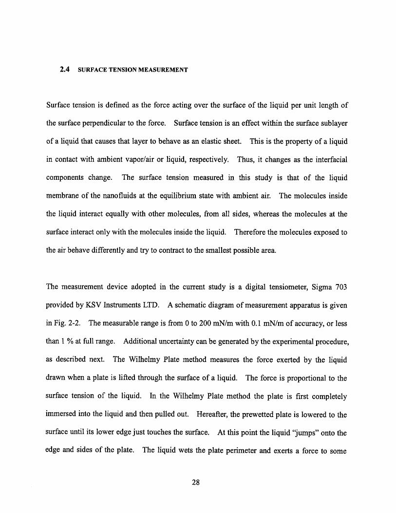
(a) 26.8' (b) 25 0
Figure 3-14 Contact angle of 0.01 v% of ZrO2 on the flat heater boiled in the 0.01 v% ZrO2
(a) 38.80 (b) 480
Figure 3-15 Contact angle of 0.001 v% of ZrO2 on the flat heater boiled in the 0.001 v% ZrO2
I

Figure 3-16 Contact angle of 0.1 v% of SiO 2 on the flat heater boiled in the 0.1 v% SiO 2
(a) 5.20
Figure 3-17 Contact angle of 0.01 v% of SiO 2 on the flat heater boiled in the 0.01 v% SiO 2
(a) 21.6' (b) 200

(a) 12.50 (b) 8.70
Figure 3-18 Contact angle of 0.01 v% of SiO2 on the flat heater boiled in the 0.01 v% SiO2

3.2.3 Scanning Electron Microscopy Results
The metal surfaces of stainless steel 316 were prepared and boiled in the nanofluids such as
alumina, zirconia, and silica dispersed in water. The SEM and EDS analyses again reveal that
some nanoparticles precipitate on the heater surface and form irregular porous structures,
which do not appear during boiling of DI water (Figs. 3-19 through 29). Therefore, with this
measurement it is confirmed that morphology of the metal surface is altered by the
precipitation of the nanoparticles. When the surface experiences a vigorous boiling condition,
the degree of the precipitation becomes more pronounced. This is of significance because
nucleate boiling heat transfer is highly affected by the surface configuration. For example, the
nucleation site density can change and thus lead to either degradation or enhancement of the
nucleate boiling heat transfer coefficient. On the other hand, the nanoparticle layer can alter
the wettability, thus affecting CHF significantly. As mentioned earlier, the change of
wettability can be quantified by measuring the change of contact angle.
According to the SEM and EDS results, some clear differences in the morphology of the
nanoparticle deposition layer are evident among the various nanofluids, as shown in Figs. 3-19
through 3-29. Such differences may depend on the kind of nanoparticles contained in the
nanofluids. These differences result in changes of surface energy and/or roughness of the
solid surface, which in turn affect the contact angle, as will be explained in Section 4....

Figure 3-19 SEM picture of bare flat heater before boiling
2 C 41 CII I II 1re 1411
zn 4.11 Cn i111 1i.8l 12.10 14411
Figure 3-20 SEM picture and EDS spectrum of flat heater boiled in the DI water
Figure 3-21 SEM picture of flat heater boiled in the 0.1 v% A12 0 3

Al
Ito 4i0: to • s 0" 4W0
Figure 3-22 SEM picture and EDS spectrum of flat heater boiled in the 0.01 v% A12 0 3
Figure 3-23 SEM picture of flat heater boiled in the 0.001 v% A120 3
Figure 3-24 SEM picture of flat heater boiled in the 0.1 v% ZrO2
......... .........

Zr
I* 4* 4* *4 3A4 t4 X44
Figure 3-25 SEM picture and EDS spectrum of flat heater boiled in the 0.01 v% ZrO2
Figure 3-26 SEM picture of flat heater boiled in the 0.001 v% ZrO2
Figure 3-27 SEM picture of flat heater boiled in the 0.1 v% SiO 2
-.. " - ". - I . - " & -
Acc V ý pý)l M.jqn Dý t WD 1 "0 Jim100kvýo ýA 101 "S316/10)OOOM
A,,c V ','.0ot Mjr1fi OfJ WD 1 100 Jimý1 204 ý'ý,31tZrWOOOI,%,
... .............

b 0 ýý,OK ,kr, ýfýý2.......... - - I
L..... ..............~** 1%' ~$* 4fl ~4 #N 4U* fl$*
Figure 3-28 SEM picture and EDS spectrum of flat heater boiled in the 0.01 v% SiO 2
Figure 3-29 SEM picture of flat heater boiled in the 0.001 v% SiO2
-A m
.
AtýcV ',ýVWWiqrt 00 WD20OWO) 100OX A
Auý V 3prit Wjqr, Dot WD 1001im20 0 PV 250,x SE 204SSý16ý:,020001%
1ý44 , a ý ý .40 $*"

3.2.4 Surface Profilometer Results
The porous layer was analyzed more quantitatively with a Tencor P-10 surface profilometer,
which gave the images shown in Fig. 3-30. The P-10 is a stylus profilometer, which uses a
sharp stylus (2 gm tip radius) to quantitatively measure surface topography. The stylus is held
at a fixed position, and the sample is scanned on a precision translation stage to do the
measurement. This system is very commonly used for measuring the thickness of thin films
using a patterned step, wafer bow for film stress analysis, and for quantitative surface
roughness across large areas.
The surface boiled in DI water is very smooth, while the surface boiled in the nanofluid
presents irregular peak-and-valley structures, which are consistent with the SEM images of Fig.
3-5 and 3-19 to 3-29. The roughness and total area of the surface boiled in nanofluid are
about twenty times and five times higher than those of the surface boiled in DI water,
respectively. The effects of such changes on the contact angle are discussed in the next
section.

(b)

Figure 3-30 Profilometer images of the flat heater surface after boiling (a) DI water, (b) 0.01
v% alumina nanofluid and (c) 0.01 v% zirconia nanofluid. The RMS roughness values are
~0.1 and -2 [m, respectively. Similar results were obtained with the other nanofluids.


4 DATA INTERPRETATION
The experiments presented in the previous Section 3 have shown that nanofluids exhibit
enhanced CHF at low nanoparticle concentrations. During nanofluid boiling the heater
surface becomes coated with a porous layer of nanoparticles, and such layer significantly
increases surface wettability. Some questions related to the above observations naturally
arise:
1) Why do nanoparticles deposit on the surface during nucleate boiling?
2) Why does the nanoparticle layer enhance wettability?
3) What effect does the nanoparticle layer have on CHF?
Questions 1 and 3 have been discussed in some detail in a separate paper [35], and only the
essential conclusions are reported here. Briefly, no significant deposition of nanoparticles
was observed while handling nanofluids or measuring their properties or even in single-phase
convective heat transfer experiments, which are being run at MIT. Thus, it is concluded that
nanoparticle deposition is a direct consequence of nucleate boiling. It is well known that a
thin liquid microlayer develops underneath a vapor bubble growing at a solid surface [20].
Therefore, it is postulated that microlayer evaporation with subsequent settlement of the
nanoparticles initially contained in it could be the reason for the formation of the porous layer.
In ref. [35] it is shown that the layer growth rate predicted on the basis of this hypothesis is
consistent with the layer thickness and experiment duration observed in our experiments. As
far as the link between wettability and CHF enhancement is concerned (Question 3), most CHF
mechanisms proposed in the literature, e.g., liquid macrolayer dryout [26,27] and hot spot

expansion [29-31], suggest that an increase in surface wettability will delay CHF. A semi-
quantitative assessment of such effect was conducted in ref. [35] and it was found that the
magnitude of the CHF enhancements reported in Fig. 3-2 is consistent with the magnitude of
the contact angle reduction reported in Table 8. Therefore, it would seem plausible to
conclude that the nanoparticles do affect CHF via a change in wettability of the boiling surface.
As part of this thesis work, the mechanism of wettability improvement (Question 2) was
analyzed carefully. To that end, Young's equation is introduced,
coso = Ysv - YSL (4-3)
which relates the static contact angle to the surface tension, a, and the so-called adhesion
tension, Ysv-YSL. The adhesion tension of water on clean steel is ~10 mN/m and its surface
tension is ~72 mN/m, so Young's equation yields a contact angle of about 820, which is in good
agreement with the measured angle of 790 (Fig. 3-9a). If the surface is not smooth, the
effective solid-liquid contact area differs from the smooth contact area. Wenzel [22] defines a
roughness factor, r, as the ratio of the effective contact area to the smooth contact area. The
free energy of the solid-liquid interface on a rough surface is then r times the free energy of a
perfectly smooth surface with the same apparent contact area. Therefore, Young's equation
needs to be modified as follows [22]:

cosO - Ysv - TSL r (4-4)
Equation (4-4) suggests that the contact angle on a rough surface depends on three parameters,
i.e., the surface tension, the adhesion tension and the roughness factor. The surface tension of
nanofluids tested in the current study was found to minimally differ from that of pure water
(Table 4 and Fig. 2-3). On the other hand the adhesion tension of water increases significantly
in going from a clean metal to an oxide, e.g., from ~10 mN/m (stainless steel) to ~60 mN/m
(alumina). Such change in adhesion tension alone reduces the contact angle to ~34 °, as
calculated from Eq. (4-4) assuming r=1. This is consistent with other studies showing that
surface oxidation decreases the contact angle [23]. The porous layer also increases the
effective contact area. Thus the roughness factor, r, is greater than unity, which also
contributes to the contact angle reduction in this study. To evaluate r, it is necessary to use the
information obtained with the profilometer. For the situation of Fig. 3-30 (a) and (b) the
estimated surface areas are about 84,000 ptm 2 (clean surface) and 470,000 ptm 2 (alumina-fouled
surface), respectively, resulting in r~5.6. For r~5.6 the contact angle decreases to -39', as
calculated from Eq. (4-4) with nominal adhesion tension (~10 mN/m) and surface tension (~72
mN/m). In summary, a simple analysis of the modified Young's equation suggests that the
enhancement in wettability (decrease in contact angle) is caused by a combination of two
effects, i.e. an increase of adhesion tension and an increase of surface roughness. Both effects
are at work and large enough to cause a pronounced reduction of the contact angle.

5 CONCLUSION AND FUTURE WORK
The pool boiling characteristics of three water-based nanofluids (silica, alumina and zirconia)
were studied experimentally. The main findings are as follows.
* Transport and thermodynamic properties of the low concentrations of nanoparticles
dispersed in water differ negligibly from those of DI water.
* Dilute dispersions of alumina, zirconia and silica nanoparticles in water exhibit
significant CHF enhancement in boiling experiments with wire heaters, up to 52 % for
alumina, 80 % for silica and up to 75 % for zirconia.
* During nucleate boiling some nanoparticles deposit on the heater surface to form a
porous layer.
* This layer improves the wettability of the surface considerably, as measured by a
marked reduction of the static contact angle. The wettability improvement is due to a
change in surface energy and roughness.
The first three findings are in agreement with other results previously reported in the nanofluid
literature. However, it is believed that this study provides an important new clue in
understanding the mechanism of CHF enhancement in nanofluids, i.e., surface wettability
changes caused by nanoparticle deposition. To elucidate such mechanism more definitively,
additional work is needed, including a thorough characterization of the layer growth during
boiling and direct measurement of the time-dependent temperature distribution on the heater

surface, which will shed light upon the effect of the porous layer on the nucleation site density
and dynamics. This should be tested in the future in order to expand the existing knowledge
base. It is also necessary to resolve the discrepancy between opposite results on the nucleate
boiling heat transfer coefficient.

References
[1] S. Choi, 1995, "Enhancing thermal conductivity of fluids with nanoparticles", in
Developments and Applications ofNon-newtonian Flows, D.A. Siginer and H.P. Wang
(Eds.), ASME, FED-Vol. 231/MD-Vol. 66, pp. 99-105.
[2] J. Buongiorno and L.-W. Hu, 2005, "Nanofluid Coolants for Advanced Nuclear Power
Plants", Paper 5705, Proceedings oflCAPP '05, Seoul, Korea, May 15-19.
[3] J. Buongiorno, L. W. Hu, S. J. Kim, R. Hannink. B. Truong, E. Forrest, "Use of
nanofluids for enhanced economics and safety of nuclear reactors", COE-INES
International Symposium, INES-2, Yokohama, Japan, November 26-30.
[4] S. M. You, J. Kim, K. H. Kim, 2003, "Effect of nanoparticles on critical heat flux of water
in pool boiling heat transfer", Applied Physics Letters, Vol. 83, No. 16, pp. 3374-3376.
[5] S. Das, N. Putra, W. Roetzel, 2003, "Pool boiling characteristics ofnano-fluids", Int. J. of
Heat and Mass Transfer, Vol. 46, pp. 851-862.
[6] P. Vassallo, R. Kumar, S. D'Amico, 2004, "Pool boiling heat transfer experiments in
silica-water nano-fluids", Int. J. of Heat and Mass Transfer, Vol. 47, pp. 407-411.
[7] T. N. Dinh, J. P. Thu, T. G. Theofanous, 2004, "Burnout in high heat flux boiling: the
hydrodynamic and physico-chemical factors", 42nd AIAA Aerospace Sciences Meeting
and Exhibit, Reno, NV, USA, January 5-6.
[8] J. H. Kim, K. H. Kim, S. M. You, 2004, "Pool boiling heat transfer in saturated
nanofluids", Proceedings oflMECE 2004, Anaheim, CA, USA, November 13-19.

[9] G. Moreno Jr., S. Oldenburg, S. M. You, J. H. Kim, 2005, "Pool boiling heat transfer of
alumina-water, zinc oxide-water and alumina-water ethylene glycol nanofluids",
Proceedings ofHT2005, San Francisco, CA, USA, July 17-22.
[10] I. C. Bang and S. H. Chang, 2005, "Boiling heat transfer performance and phenomena of
A120 3-water nano-fluids from a plain surface in a pool", Int. J. of Heat and Mass Transfer,
Vol. 48, pp. 2407-2419.
[11] D. Milanova and R. Kumar, 2005, "Role of ions in pool boiling heat transfer of pure and
silica nanofluids", Applied Physics Letters, Vol. 87, 233107.
[12] D. Wen and Y. Ding, 2005, "Experimental investigation into the pool boiling heat transfer
of aqueous based y-alumina nanofluids", Journal of Nanoparticle Research, Vol. 7, pp.
265-274.
[13] H. Kim, J. Kim, M. Kim, 2006, "Experimental study on the characteristics and mechanism
of pool boiling CHF enhancement using nano-fluids", ECI International Conference on
Boiling Heat Transfer, Spoleto, Italy, May 7-12.
[14] H. Kim, J. Kim, M. Kim, 2006, "Experimental study on CHF characteristics of water-TiO 2
nano-fluids", Nuclear Engineering and Technology, Vol. 38, No. 1, pp. 61-68.
[15] Z. -H. Liu, Y. -H. Qiu, 2007, "Boiling heat transfer characteristics of nanofluids jet
impingement on a plate", Heat and Mass Transfer, Vol. 43, 699-706.
[16] K. -J. Park, D. Jung, 2007, "Enhancement of nucleate boiling heat transfer using carbon
nanotubes", Int. J. ofHeat and Mass Transfer, in press.
[17] Y. A. Qengel, M. A. Boles, 2002, Thermodynamics, An Engineering Approach, 4th Ed.,
McGraw Hill.
[18] D. Milanova, R. Kumar, S. Kuchibhatla, S. Seal, 2006, "Heat transfer behavior of oxide
nanoparticles in pool boiling experiment", Proc. of 4 th International Conference on
Nanochannels, Microchannels and Minichannels, Limerick, Ireland, June 19-21.
[19] D. T. Wasan and A. D. Nikolov, 2003, "Spreading of nanofluids on solids", Nature, 423, 8,
156.
[20] J.G. Collier and J.R. Thome, 1996, Convective Boiling and Condensation, 3 rd Ed., Oxford
Science Publications.
[21] R. Cole and W. Rosenhow, 1969, "Correlation of bubble departure diameters for boiling
of saturated liquids", Chem. Eng. Prog. Symp. Ser, Vol. 65, No. 92, pp. 211-213.
[22] R. N. Wenzel, 1949, "Surface roughness and contact angle (letter)", J. Physical Colloid
Chemistry, 53, 9, 1466.
[23] C. H. Wang and V. K. Dhir, 1993, "Effect of surface wettability on active nucleation site
density during pool boiling of water on a vertical surface", J. Heat Transfer, Vol. 115, pp.
659-669.
[24] S. S. Kutateladze, 1952, "Heat Transfer in Condensation and Boiling", AEC-TR-3770.
[25] N. Zuber, 1959, "Hydrodynamic Aspects of Boiling Heat Transfer", AECU-4439.
[26] Y. Haramura and Y. Katto, 1983, "A new hydrodynamic model of CHF applicable widely
to both pool and forced convection boiling on submerged bodies in saturated liquids", Int.
J. of Heat and Mass Transfer, Vol. 26, pp. 389-399.
[27] P. Sadasivan, P. R. Chappidi, C. Unal, and R. A. Nelson, 1992, "Possible Mechanisms of
Macrolayer Formation", Pool and External Flow Boiling (ASME 1992) p. 135.

[28] Y. Katto and S. Yokoya, 1968, "Principal mechanism of boiling crisis in pool boiling", Int.
J. Heat Mass Transfer, Vol. 11, pp. 993-1002.
[29] T. G. Theofanous et al., 2002, "The boiling crisis phenomenon. Part II: dryout dynamics
and burnout", Experimental Thermal and Fluid Science, Vol. 26, pp. 793-810.
[30] M. Arik and A. Bar-Cohen, 2003, "Effusivity-based correlation of surface property
effects in pool boiling CHF of dielectric liquids", Int. J. Heat Mass Transfer, Vol. 46, pp.
3755-3764.
[31] T. G. Theofanous and T. N. Dinh, 2006, "High heat flux boiling and burnout as
microphysical phenomena: mounting evidence and opportunities", Multiphase Science
and Technology, Vol. 18, No. 1, pp. 1-26.
[32] S. V. Gupta, 2004, "Capillary action in narrow and wide tubes - a unified approach",
Metrologia, Vol. 41, pp. 361-364.
[33] W. Rosenhow and P. Griffith, 1956, "Correlation of maximum heat flux data for boiling
of saturated liquids", Chem. Eng. Prog. Symp. Ser. Vol. 52, No. 18, pp. 47-49.
[34] N. Kolev, 2002, "How accurately can we predict nucleate boiling?", in Multiphase Flow
Dynamics 2, Springer.
[35] S. J. Kim, I. C. Bang, J. Buongiorno, L. W. Hu, 2007, "Surface wettability change during
pool boiling of nanofluids and its effect on critical heat flux", Int. J. of Heat and Mass
Transfer, in press.
[36] B. Chu, 1991, Laser Light Scattering: Basic Principles and Practice, Academic Press,
Boston.

[37] P. J. Freud, M. N. Freud, 1992, A New Approach to Particle Sizing by Dynamic Light
Scattering, Microtrac. Inc.