Polynomial Representation for Persistence Diagram

Zhichao Wang1∗ Qian Li2∗ Gang Li3 Guandong Xu2

1School of Electrical Engineering and Telecommunications, University of New South Wales, Australia

2Advanced Analytics Institute, University of Technology Sydney, Australia

3School of Information Technology, Deakin University, Geelong, VIC 3216, Australia

zhichao.wang2@unsw.edu.au {qian.li, guandong.xu}@uts.edu.au gang.li@deakin.edu.au

Abstract

Persistence diagram (PD) has been considered as a com-

pact descriptor for topological data analysis (TDA). Unfor-

tunately, PD cannot be directly used in machine learning

methods since it is a multiset of points. Recent efforts have

been devoted to transforming PDs into vectors to accom-

modate machine learning methods. However, they share

one common shortcoming: the mapping of PDs to a feature

representation depends on a pre-defined polynomial. To ad-

dress this limitation, this paper proposes an algebraic rep-

resentation for PDs, i.e., polynomial representation. In this

work, we discover a set of general polynomials that van-

ish on vectorized PDs and extract the task-adapted feature

representation from these polynomials. We also prove two

attractive properties of the proposed polynomial represen-

tation, i.e., stability and linear separability. Experiments

also show that our method compares favorably with state-

of-the-art TDA methods.

1. Introduction

As a bridge between algebraic topology and statistical

methods, topological data analysis (TDA) extracts the topo-

logical features that are complementary to statistical quanti-

ties [33, 36]. In the past several years, TDA has found many

applications in areas including bioinformatics [6, 31, 38],

computer vision [5, 14, 25, 28], audio signals [4, 29] and

natural language processing [18, 40]. As one common

approach to TDA, persistent homology captures the char-

acteristics of data by the scales at which topological fea-

tures (connected component, cycle, void, etc.) are born and

the scales at which they die. A standard way to represent

the persistent homology is through the persistence diagram

(PD), which encodes the lifespan of every topological fea-

ture [13, 36]. However, PD cannot be straightforwardly

∗Equal contribution

adopted in standard machine learning methods, because it

is not in the vector space [1, 7].

Related work. To address this issue, considerable ef-

forts have been devoted to mapping PDs into a vector space,

and existing work can be categorized into three classes.

Methods in the first class express PDs in the Hilbert space

via kernel functions [7, 10, 26, 35]. For instance, a multi-

scale heat kernel is defined for PDs through a L2-valued

feature mapping, which thus can be used with the support

vector machine (SVM) [35]. Alternately, a weighted Gaus-

sian kernel is proposed to treat a PD as a discrete measure,

and to control the effect of persistence in the PD [26]. The

sliced Wasserstein kernel is also a Gaussian-type kernel de-

fined by a modified Wasserstein distance between PDs [7].

Methods in the second class directly vectorize PDs in the

Euclidean space [1, 2, 11, 15]. For instance, the persis-

tence image [1] constructs Rn representation by integrating

a weighted density estimate of the PD into a persistence sur-

face. Persistence square-root representation [2] models the

PD as a 2D probability density function on the tangent vec-

tor space of Riemannian manifold. Deep neural networks is

adopted to vectorizes PDs by defining input layer with sta-

ble property [24]. Methods in the third class represent PDs

in the function space. For example, persistence landscapes

(PLs) [11] are developed to construct the piecewise linear

functions on PDs for further data analysis tasks. Another

work [15] transforms PDs into complex polynomials of the

function space.

Above vectorization methods consider the resulting vec-

tors of PDs as the feature inputs for machine learning, and

some of them achieve provable stability under the pertur-

bations in PDs. However, most existing works focus on

defining the polynomials with specific form (e.g. kernel

map) for PDs, which may be suboptimum. Instead of pre-

defined polynomials, how to extract more flexible or prefer-

able polynomials from PDs for constructing discriminative

features remains largely unexplored.

6123

Figure 1. An example of polynomial representation for PDs. Assume m PDs {Di}1≤i≤m belong to the same class, our method first derives

m stable persistence vectors {vi}1≤i≤m from those PDs. Assume that two polynomials approximately vanish on those m persistence

vectors, i.e., f1(v) ≈ 0 and f2(v) ≈ 0 for all v. Using those vanishing polynomials, our method can define the polynomial representation

for PDs, which is proved to be linearly separable.

Contributions. To address these limitations, this paper

proposes a task-oriented algebraic representation for PDs,

namely polynomial representation, which extracts the sta-

ble and linearly separable features for PDs. As shown in

Fig. 1, the proposed polynomial representation consists of

two steps: stable persistence vectorization and representa-

tion with vanishing polynomials.

First, stable persistence vectorization transforms a PD

into a persistence vector while maintaining interpretable

connections. As a theoretical contribution, the persistence

vector is proved to be stable with respect to perturbations

in PDs. Second, the persistence vector is treated as the root

of some general polynomials to construct the polynomial

representation with the forms of nonlinear curves, surfaces

and their unions. By exploiting the underlying nonlinear

nature, representation with vanishing polynomials can ex-

tract the task-specific and discriminative features from the

persistence vector. This also offers greater flexibility and

representational power by deriving linearly separable fea-

ture, which can obviously improve the classification per-

formance. In addition, an efficient algorithm is proposed to

compute the polynomial representation from the persistence

vectors. Numerical experiments on topological data analy-

sis demonstrate the favorable performance of the proposed

method.

2. Preliminary on Persistence Diagram

In this section, we give a brief overview of the persis-

tence diagram, and leave more details in the supplementary.

A comprehensive introduction can be found in [12, 13].

Topological data analysis (TDA) aims to infer com-

plex topological features (connected components, cavities

and higher-dimensional holes) directly from underlying

data [16, 18]. Machine learning methods can also uncover

the geometric structure of data, but they can only identify

0-dimensional topological structure, i.e., connected com-

ponents. Unsupervised learning or clustering in machine

Figure 2. An example of persistence diagram.

learning can be viewed as the 0-dimensional holes of topo-

logical inference, i.e., the connectivity of the data. In gen-

eral, for a more general topological space embedded in d-

dimensional Euclidean space, there are d-different types of

holes with dimension from 0 to d�1. For example, a sphere

encloses a 2-dimensional hole while a circle encloses a 1-

dimensional hole.

TDA can track how the topological features appear and

disappear in a nested sequence of topological spaces. A

standard descriptor to represent such topological evolution

is persistence diagram (PD) [12, 13], which is in fact a

multi-set of points in a plane. Each point (b, d) corresponds

to the lifespan of one topological feature, where b and dare its birth time and death time, respectively. Points are

entirely located in the half-plane above the diagonal, since

the death time always occurs after the birth time.

Fig. 2 gives an example of PD with respect to a height

function f on a surface. One way to understand the function

f is through the topology of its sublevel sets f−1((�1, t]).The sublevel set f−1((�1, t]) can record such topologi-

cal events, i.e, the cycle may create or merge when varying

t from �1 to 1. We start with the 1-dimensional topo-

logical feature (i.e., cycle) carried by the sublevel sets. For

instance, a point (b, d) is depicted in the PD corresponding

to the 1-dimensional topological feature �1. When t goes

6124

through the height value b, the sublevel sets f−1((�1, b])that were homeomorphic to two discs become homeomor-

phic to the disjoint union of a disc and an annulus, creating

a first cycle homologous to �1. These two created cycles

are never filled before t reaches the end of the filtration d.

The interval between the birth time b and the death time

d reflects the persistence (lifespan) of �1. To understand

the topological feature with more than one dimension, the

preliminary of algebraic topology is required, please refer

to [18, 22] for details. Points far from the diagonal rep-

resent the persistent topological features with long persis-

tences, while points close to the diagonal can be considered

as topological noise. The supplementary also provides an

example of PD construction from point cloud data.

A popular metric to measure the similarity between two

PDs is p-Wasserstein distance[34]. Points on the diagonal

of PD are considered as a part of PD such that there exists

bijections between two PDs [13, 35]. In general, this metric

is expressed by minimizing the distance of any two corre-

sponding points, over all bijections between two PDs.

Definition 1 [34] Given two PDs D1 and D2, let � be a

bijection between D1 and D2. For any p > 0, the p-

Wasserstein distance is

dW,p(D1,D2) = infγ:D1→D2

X

u∈D1

ku� �(u)kp∞

!1/p

(1)

Note that a bijection � exists by matching points in D1 with

points in D2 such that each point in D1 (resp. in D2 ) has

to be matched, either to a unique point in D2 (resp. in D2

), or to its nearest neighbor in the diagonal. One reason for

the popularity of PDs in topological data analysis is that the

transformation of a topological data into a PD is stable with

respect to p-Wasserstein distance [13, 35].

PDs for machine learning. In fact, the space of PDs

is a metric space with the p-Wasserstein distance [13, 35].

However, this metric space is neither a Euclidean space nor

a Hilbert space [1, 7]. For machine learning methods such

as SVM or PCA, the input data is supposed to be in the

Euclidean space or Hilbert space. Therefore, PDs cannot

be directly used as inputs for a variety of machine learning

methods. To analyze topological features encoded in PDs,

most statistical research works convert the PD into a vec-

tor [1, 7, 26, 36].

3. Stable persistence vectorization

The first part of the proposed polynomial representation

is stable persistence vectorization. This novel vectorization

method transforms the PD into a Euclidean vector while

maintaining the interpretable connection with the original

PD. The proposed vectorization is stable with respect to per-

turbations of PDs and also efficient to compute.

Recall that PD is a 2-dimensional plane with a set of

points. A point (ux, uy) represents that a topological fea-

ture is born at time ux and dies at uy . All points (ux, uy) lie

above the diagonal, since the birth must precede the death.

Hence, uy � ux defines the persistence of the topological

feature. The point with a long persistence represents an

important topological feature, while the point with a short

persistence may represent the topological noise. To mea-

sure the importance of points in PDs, we propose a flexible

weighting function as

!(ux, uy) = arctan(C(uy � ux)2) (2)

where C is a non-negative parameter. The weighting func-

tion is non-decreasing with respect to the persistence of

each PD point, which gives large weights for points with

long-persistences to indicate its high significance in PDs.

More importantly, arctan is a bounded and continuous

function, which is vital to guarantee the stability of the vec-

torization of PDs. Parameter C ensures that points with

long persistences will have large weights, while points with

short persistences will have small weights.

Based on the weight function, we construct a mapping

from the PD to a finite-dimensional vector. To ensure that

the resulting vector is stable w.r.t. permutations of PDs, the

mapping needs to be Lipschitz continuous [13]. A standard

strategy is to construct a kernel mapping via an exponential

function [26, 35]. However, the kernel mapping is usually

inefficient to compute. For computational efficiency, we use

a simple exponential function to define a Lipschitz scalar

function ⇢ : R! R as

⇢D(z) =X

(ux,uy)∈D

!(ux, uy)e− (ux−z)2

σ2

(3)

where � is a width parameter. Eq. (3) defines the mean of

exponential function ux. Alternatively, one can use uy � zor (ux + uy)/2 � z as the mean. All these choices do not

change the stability of persistence vector with only a slight

modification to the constants. With this scalar function, we

define a novel persistence vector derived from a PD.

Definition 2 (Persistence vector) Define the range [a, b]that contains the ranges of the birth/death times of all points

in the PDs. Let I = b � a, the n-dimensional persistence

vector of a PD D is defined as

vD :=I

n· [⇢D(a+

I

n), ⇢D(a+

2I

n), ..., ⇢D(a+

nI

n)] (4)

Note that the interval [a, b] is defined to involve the

ranges of birth/death times of points in all the PDs. For

a specific PD D, its persistence vector vD with dimension

n is generated by computing the scalar function ⇢ over the

discretized interval [a, b]. In that way, v can evenly explore

6125

the complete spatial information in PDs by uniformly being

increased in the PD. More importantly, the ingredient I/nis crucial to ensure that persistence vector v is stable with

respect to small perturbations of PDs. In the following, the

stability of persistence vector is given in Theorem 1.

Lemma 1 Let u = (ux, uy) 2 D1 be the point in PD, the

point v 2 D2 be the perturbed version of u. For ⇢ in Eq. (3),

we have an exponential function gux(z) = e−

(ux−z)2

σ2 and

a weighting function !(u) = arctan(C(uy � ux)2). Let

K =p2⇣

1 +√π

σ

⌘

, then we have

Z ∞

−∞|!(u)gux

(z)� !(v)gvx(z)| dz Kku� vk∞ (5)

Proof See proof in the supplement.

With Lemma 1 in mind, we turn to prove the persistence

vector is stable w.r.t. 1-Wasserstein distance between PDs.

Theorem 1 (Stability Theorem) The persistence vector v

is stable w.r.t. the 1-Wasserstein distance dW,1 between

their PDs. In particular,

kvD1� vD2

k1 p2

✓

1 +

p⇡

�

◆

· dW,1(D1,D2)

kvD1 � vD2k2 p2

✓

1 +

p⇡

�

◆

· dW,1(D1,D2)

kvD1 � vD2k∞ p2

✓

1 +

p⇡

�

◆

· dW,1(D1,D2)

Proof 1-Wasserstein distance states that a bijection is re-

quired when comparing two PDs, i.e., D1 and D2. Points on

the diagonal are considered as a part of every persistence

diagram D such that there exists a bijection � generating

�(u) = (vx, vy) 2 D2 for u = (ux, uy) 2 D1.

kvD1� vD2

k1 =I

n

nX

i=1

|⇢D1(zi)� ⇢D2

(zi)|

Z ∞

−∞|⇢D1

(z)� ⇢D2(z)|dz

=

Z ∞

−∞

�

�

�

�

�

�

X

u∈D1

!(u)gux(z)�

X

γ(u)∈D2

!(v)gvx(z)

�

�

�

�

�

�

dz

X

u∈D1

Z ∞

−∞|!(u)gux

(z)� !(v)gvx(z)| dz

p2

✓

1 +

p⇡

�

◆

· dW,1(D1,D2) (By Lemma 1)

We now have the following relation

kvD1 � vD2k1 p2

✓

1 +

p⇡

�

◆

dW,1(D1,D2)

For vectors in Rn, l2-norm and l1-norm follow

kvD1� vD2

k2 kvD1� vD2

k1

Similarly, we have

kvD1� vD2

k∞ kvD1� vD2

k1

Theorem 1 then follows.

Remark We need to clarify that the stability of persis-

tence vector is not specific to the scalar function ⇢ defined

in Eq (3). Our choice of ⇢ is a possible representative func-

tion that is easy to compute meanwhile has the following

two conditions. First, the scalar function ⇢ satisfies the con-

dition (5) in Lemma 1 can produce the stability theorem for

persistence vectors. Second, the weight in ⇢ should be zero

for the point in the diagonal of persistence diagram, which

implies that this point is the topological noise and should be

neglected in practical.

4. Representation with vanishing polynomials

Stability is not enough for machine learning. The

persistence vectors in Eq. (4) with stability property can

be considered as the feature representation of PDs. More

importantly, the separability of such feature representation

should be theoretically guaranteed when plugged into ma-

chine learning methods.

To obtain the linear separable features from persistence

vectors, Gaussian or polynomial kernel is the standard way

to map the vector space to the lifted space. However, the

polynomial mapping of kernel needs to be pre-defined and

therefore is suboptimal to any specific learning tasks. More-

over, the selection of appropriate kernel for task-oriented

feature representation is tricky so as to achieve the satis-

factory classification performance. To alleviate these prob-

lems, this section aims to learn the task-adapted and lin-

early separable feature representation, which captures the

discriminative structure of the persistence vector. We also

experimentally confirm the discriminative power of the pro-

posed method and show that it outperforms conventional

kernel methods.

4.1. Problem statement

In the following, we denote a persistence vector set as

V, in which each v 2 V is a persistence vector that is de-

rived from a persistence diagram as in Eq. (4). Inspired by

the vanishing ideal in [17, 23, 30], our approach builds upon

the following assumption: persistence vectors in V are re-

garded as the roots of a polynomial system. This assump-

tion is useful to derive the vanishing polynomial set, which

allows us to obtain the linearly separable feature underlying

the persistence vectors.

6126

Definition 3 The vanishing polynomial set I(V) is defined

as a set of polynomials vanishing on persistence vectors V.

I(V) = {f 2 R[v] : f(v) = 0 for all v 2 V} (6)

where R[v] denotes the space of all polynomials with real

coefficients in vector v.

Remark. With the definition of vanishing polynomial

set, we can extract the linearly separable feature from PDs

through the following two important procedures: The first

step is to construct the vanishing polynomial set for the per-

sistence vectors using Algorithm 1. The vanishing polyno-

mial set can characterize the discriminative algebraic struc-

ture underlying the persistence vectors. By using the van-

ishing polynomial set, the second step is to derive the poly-

nomial representation from for persistence vectors. We can

prove that the resulting polynomial representation is lin-

early separable. This section also shows how the polyno-

mial representation can be used for classification.

4.2. Vanishing polynomials of persistence vectors

We first give a step by step formulation for vanishing

polynomials. Any degree-d polynomial can be decomposed

into a sum of homogeneous polynomials as

f =X

1≤i≤d

wiφTi = (w1, · · · ,wd)(φ1, · · · ,φd)

T = wΦ

(7)

where φd is a vector of degree-d homogeneous monomi-

als, and wd is its coefficient vector. For example, given

a 2-dimensional persistence vector v = (x, y), f1(v) =�x + 3y + 6x2 � 2xy + 7y2 = 0 in Fig. 1 induces

w1 = (�1, 3), φ1(v) = (x, y), w2 = (6,�2, 7) and

φ2(v) = (x2, xy, y2). In fact, φd is a degree-d Veronese

map [21]:

φd : (x1, · · · , xk) 7! (· · · , xi11 · · ·xik

k , · · · ) (8)

where i1 + · · · + ik = d means that the degree-d Veronese

map sends [x1, · · · , xk] to all possible monomials of total

degree d. For example, φ2(v) is the degree-2 Veronese map

of x and y.

Degree-d polynomial matrix. Recall that our goal is to

find a set of vanishing polynomials for persistence vectors.

Given a set of persistence vectors V = {v1, · · · ,vm} and

polynomials Φ = (φ1,φ2, · · · ,φd)T , we first construct the

following polynomial matrix

Φ(V) = [Φ(v1), · · · ,Φ(vm)]

=

0

B

B

@

φT1 (v1), φT

1 (v2), · · · φT1 (vm)

φT2 (v1), φT

2 (v2), · · · φT2 (vm)

· · · · · · · · · · · ·

φTd (v1), φT

d (v2), · · · φTd (vm)

1

C

C

A

(9)

Algorithm 1 Vanishing polynomial set

Input: persistence diagrams {D1, · · · ,Dm} within the

same class, n, d and ✏

Initialize: a set of persistence vectors V ={v1, · · · ,vm} 2 R

m×n via Eq. (4)

1: Build the degree-d polynomial matrix Φ(V) via

Eq. (9)

2: Find null space by performing SVD on Φ(V) =UΣW

T via Eq. (11)

3: Compute the vanishing polynomial set with tolerance

✏, i.e.,

I(V) {Φ(V)Wi,�i < ✏}

Output: Vanishing polynomials I(V)

where �d(vi) is computed by the degree-d Veronese map

on vi 2 V according to Eq. (8). We restrict �d(vi) to the

lower-degree polynomials, otherwise the higher degree will

overfit the data.

Null space of Φ(V). Eq. (7) implies that f vanishes on

persistence vectors V if and only if the coefficient vector

lies in the null space of Φ(V) in Eq. (9). That means the

following relationship

f(V) = WΦ(V) = 0 () W 2 null(Φ(V)) (10)

A straightforward way to compute the null space of ma-

trix is through singular value decomposition (SVD)

Φ(V) = UΣWT (11)

Multiply Eq. (11) by an orthogonal matrix W and obtain

Φ(V)W = UΣ (12)

We focus on the i-th column of W and U, i.e., Φ(V)Wi =Ui�i. Denote that wi and ui are the i-th singular vector of

W and U respectively. Scalar �i is the i-th singular value

in the diagonal matrix Σ.

Compute vanishing polynomials. If the i-th singular

value �i = 0, its singular vector Wi lies in the null space

of Φ(V). We can regard Wi as a coefficient vector of the

linear combination of the polynomials in Φ. Accordingly,

the vanishing polynomials for V can be computed as

I(V) = {Φ(V)Wi | Wi is a singular vector w.r.t. �i = 0}(13)

The size of I(V) is equivalent to the number of zero sin-

gular values �i in the diagonal matrix Σ, according to

Eq. (13). Therefore, we have the following relation

|I(V)| = #{�i = 0} rank(Σ) = rank(Φ(V))

min(d,m) m(14)

6127

which implies that the number of vanishing polynomials on

V is less than the sample size m. The pseudo-code of com-

puting I(V) is summarized in Algorithm 1.

Remark. Perturbations in the persistence vectors V are

unavoidable due to the noisy PDs. It is unreasonable to seek

zero singular values of Φ(V). Instead, we choose the right

singular vectors of Φ(V) corresponding to near-zero singu-

lar values �i with ✏-tolerance.

4.3. Linearly separable feature

Given s different classes of topological data, we can

compute their corresponding s sets of PDs using the soft-

ware DIPHA [3]. With these prepared PDs, our method

begins with computing s categories of the persistence vec-

tors {V1, · · · ,Vs} via the persistence vectorization (Def-

inition 2). Accordingly, s vanishing polynomial sets

{I1(·), · · · , Is(·)} can be derived by Algorithm 1. We now

demonstrate that one can represent a persistence vector v

with these vanishing polynomial sets.

Definition 4 The polynomial representation is a s-

dimensional Euclidean vector that can be obtained through

the mapping

v 7! (kI1(v)k2, kI2(v)k2, · · · , kIs(v)k2) 2 Rs (15)

where v is the persistence vector, kIk(·)k2 is a vector norm

and Ik(·) = {f1, f2, · · · , f|Ik|} (computed by Algorithm 1)

denotes the vanishing polynomial set of the k-th class per-

sistence vectors.

The polynomial representation is a Euclidean vector with

one significant property: if the persistence vector v belongs

to the k-th class, then the k-th component kIk(v)k2 of its

polynomial representation is zero. In contrast, other com-

ponents kIl(v)k2 are non-zero, where l 6= k. From this

property, we can prove that the polynomial representation

is linearly separable among different classes of persistence

vectors.

Theorem 2 The polynomial representation defined as

Eq. (15) is linearly separable in the feature space

(kI1(·)k2, · · · , kIs(·)k2).

Proof Case 1 (s = 2): We assume two classes of per-

sistence vectors, denoted as V1 and V2. Their vanishing

polynomial sets are I1(·) and I2(·), respectively. The poly-

nomial representation of v 2 V1 and κ 2 V2 are

⇢

v 7! (kI1(v)k2, kI2(v)k2)κ 7! (kI1(κ)k2, kI2(κ)k2) (16)

Since all v 2 V1 are defined as the common roots of I1(·)rather than I2(·). Similarly, all κ 2 V2 are defined as the

common roots of I2(·) rather than I1(·). We can induce

that

⇢

kI1(v)k2 = 0 and kI2(v)k2 > �1 > 0kI2(κ)k2 = 0 and kI1(κ)k2 > �2 > 0

(17)

Based on Eq. (17), we use two weight parameters �1 > 0and �2 < 0 to obtain two inequalities.

⇢

�1kI1(v)k2 + �2kI2(v)k2 < �2�1 < 0�1kI1(κ)k2 + �2kI2(κ)k2 > �1�2 > 0

(18)

Eq. (18) indicates that the polynomial representations of v

and κ can be linearly separated by the classifier (�1,�2).Case 2 (s > 2): Without loss of generality, we use the

one-vs-the-rest strategy to prove the multiclass classifica-

tion case. We randomly choose one class of persistence

vectors as the first class and consider the rest as the sec-

ond class. The multi-class problem is transformed into a

two-class problem, which can be proved as in Case 1.

5. Numerical results

Our work (or other TDA works) is actually complemen-

tary to traditional features rather than competing with them,

and that is why we do not compare it with well-known

feature representations (e.g., CNN). We follow the general

practise in TDA research [7, 8, 26] and carry out a series

of experiments comparing with popular TDA methods on

tasks including texture recognition and protein analysis.

We compare our method with several popular TDA

methods on classical benchmark datasets. For the input

topological data, we construct their PDs of different classes

using the software DIPHA [3], evaluate the discriminative

capability of state-of-the-art TDA methods, and reveal the

most effective vectorization of PDs when combined with

machine learning techniques, e.g., LIBSVM [9] in our ex-

periments. Parameter setting of all comparison methods

will be first described.

PSS. Persistence scale space kernel [35] utilizes a multi-

scale kernel function and maps PD into a Hilbert space that

is appropriate for machine learning algorithms. This kernel

function is defined by the solutions of heat diffusion equa-

tion at the points of PD. We choose the kernel scale param-

eter � from {10−3, 10−2, 0.2, 1, 10, 50, 102, 103}.

PSR. Persistence square-root representation [2] models

a PD as a probability density function (pdf) on the Hilbert

Sphere. It then discretizes the pdf into a K ⇥ K grid. A

smaller value of K reduces the accuracy, and a larger Kimproves the accuracy as well as the computational cost.

Parameter K is chosen from the set {5, 10, 20, 50, 75, 100}.

PI. Persistence image [1] represents a PD as

a finite-dimensional vector that is derived by the

weighted kernel density estimation. The resolution

parameter of the persistence image is selected from

6128

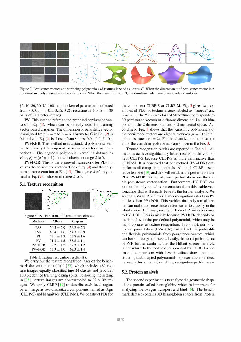
Figure 3. Persistence vectors and vanishing polynomials of textures labeled as “canvas”. When the dimension n of persistence vector is 2,

the vanishing polynomials are algebraic curves. When the dimension n = 3, the vanishing polynomials are algebraic surfaces.

{5, 10, 20, 50, 75, 100} and the kernel parameter is selected

from {0.01, 0.05, 0.1, 0.15, 0.2}, resulting in 6 ⇥ 5 = 30pairs of parameter settings.

PV. This method refers to the proposed persistence vec-

tors in Eq. (4), which can be directly used for training

vector-based classifier. The dimension of persistence vector

is assigned from n = 2 to n = 5. Parameter C in Eq. (2) is

0.1 and � in Eq. (3) is chosen from values{0.01, 0.5, 2, 10}.

PV+KER. This method uses a standard polynomial ker-

nel to classify the proposed persistence vectors for com-

parison. The degree-t polynomial kernel is defined as

K(x, y) = (xT y + 1)t and t is chosen in range 2 to 5.

PV+POR. This is the proposed framework for PDs in-

volves the persistence vectorization of Eq. (4) and the poly-

nomial representation of Eq. (15). The degree d of polyno-

mial in Eq. (9) is chosen in range 2 to 5.

5.1. Texture recognition

Figure 5. Two PDs from different texture classes.

Methods Clbp-s Clbp-m

PSS 70.5 ± 2.9 56.2 ± 2.3

PSR 68.4 ± 1.6 54.3 ± 0.9

PI 72.1 ± 1.3 57.8 ± 1.6

PV 71.8 ± 1.5 55.8 ± 1.1

PV+KER 72.2 ± 1.2 57.3 ± 1.2

PV+POR 75.3 ± 1.0 62.3 ± 1.4

Table 1. Texture recognition results (%).We carry out the texture recognition tasks on the bench-

mark dataset OUTEX00000 [32], which includes 480 tex-

ture images equally classified into 24 classes and provides

100 predefined training/testing splits. Following the setting

in [35], texture images are downsampled to 32 ⇥ 32 im-

ages. We apply CLBP [19] to describe each local region

on an image as two discretized components named as Sign

(CLBP-S) and Magnitude (CLBP-M). We construct PDs for

the component CLBP-S or CLBP-M. Fig. 5 gives two ex-

amples of PDs for texture images labeled as “canvas” and

“carpet”. The “canvas” class of 20 textures corresponds to

20 persistence vectors of different dimension, i.e., 20 blue

points in the 2-dimensional and 3-dimensional space. Ac-

cordingly, Fig. 3 shows that the vanishing polynomials of

the persistence vectors are algebraic curves (n = 2) and al-

gebraic surfaces (n = 3). For the visualization purpose, not

all of the vanishing polynomials are shown in the Fig. 3.

Texture recognition results are reported in Table 1. All

methods achieve significantly better results on the compo-

nent CLBP-S because CLBP-S is more informative than

CLBP-M. It is observed that our method (PV+POR) out-

performs all comparison methods. Although CLBP is sen-

sitive to noise [19] and this will result in the perturbations in

PDs, PV+POR can remedy such perturbations via the sta-

ble persistence vectorization. Furthermore, PV+POR can

extract the polynomial representation from this stable vec-

torization that will greatly benefits the further analysis. We

see that PV+KER achieves higher recognition rates than PV

but less than PV+POR. This verifies that polynomial ker-

nel can make the persistence vector easier to classify in the

lifted space. However, results of PV+KER are suboptimal

to PV+POR. This is mainly because PV+KER depends on

the kernel with the pre-defined polynomial, which may be

inappropriate for texture recognition. In contrast, our poly-

nomial presentation (PV+POR) can extract the preferable

and flexible polynomials from persistence vectors, which

can benefit recognition tasks. Lastly, the worst performance

of PSR further confirms that the Hilbert sphere manifold

is not robust to the perturbations caused by CLBP. Exper-

imental comparisons with these baselines shows that con-

structing task adapted polynomials representation is indeed

necessary for achieving satisfying recognition performance.

5.2. Protein analysis

The second experiment is to analyze the geometric shape

of the protein called hemoglobin, which is important for

analyzing the oxygen transport and bind [6]. The bench-

mark dataset contains 3D hemoglobin shapes from Protein

6129

Figure 4. Persistence vectors and vanishing polynomials of proteins labeled as “Relaxed”. When the dimension n of persistence vector is

2, the vanish polynomials are algebraic curves. When the dimension n = 3, the vanish polynomials are algebraic surfaces.

Data Bank (PDB) 1. These hemoglobin shapes exist in one

of two conformations known as the Relaxed form and the

Taut form. In total, we use 9 Relaxed forms and 10 Taut

forms of hemoglobin. We select one hemoglobin data from

each form as testing data, and use the remaining as training

data. Consequently, 90 runs are performed and the accuracy

is calculated via the cross-validation. Fig. 6 gives two ex-

amples of PDs for hemoglobin proteins labelling Taut form

and Relaxed form. Fig. 4 shows some examples of vanish-

ing polynomials for Relaxed class. When the dimension nof persistence vector is 2, the vanishing polynomials are al-

gebraic curves. When the dimension n = 3, the vanishing

polynomials are algebraic surfaces.

Figure 6. Two PDs from different protein classes.

Methods Relaxed Taut

PSS 83.2 ± 1.6 92.3 ± 1.4

PSR 82.4 ± 0.8 93.7 ± 1.2

PI 85.1 ± 1.2 92.7 ± 0.9

PV 82.9 ± 1.4 92.1 ± 1.6

PV+KER 84.2 ± 1.3 92.6 ± 1.4

PV+POR 86.7 ± 0.9 94.7 ± 0.8

Table 2. Protein recognition results (%).

The averaged classification accuracy of 90 independent

runs is reported in Table 2. Our method (PV+POR) achieves

the highest average accuracy in both protein forms, with the

accuracy of 86.7% for the Relaxed form and 94.7% for the

Taut form. Note that the expensive cost of protein collection

leads to those small-scale benchmark datasets for protein

analysis. As we know, the small-scale data are not preferred

when training the classifier. Our method alleviates this is-

sue by extracting linear separable feature that is easy to be

distinguished among different classes of proteins. In con-

1https://www.rcsb.org

trast, the compared TDA methods conventionally assume

that the long-persistent topological components are signifi-

cant for classification, while the short-persistent topological

components should be discarded as noise. However, both

the global and the local features are equally important to

characterize different proteins structures [37, 39].

6. Conclusion

Persistent diagram (PD) is a topological data analysis

tool which performs multi-scale analysis on topological

structures. This paper proposes a novel algebraic represen-

tation for PDs and complements standard feature represen-

tations for machine learning, which is proved to be stable

and linearly separable. Specifically, an efficient and stable

persistence vectorization is proposed to transform PDs into

the Euclidean vectors called the persistence vectors. Persis-

tence vector preserves the significance of each topological

feature encoded in PDs, which is proved to be stable with

the perturbations of PDs. Compared with existing TDA

methods which only provide the pre-defined feature map,

our method goes beyond and exploits the flexible polyno-

mial representation from the persistence vector. In addition,

a simple approximation algorithm is proposed to compute

the polynomial representation. Most significantly, we can

prove that the proposed polynomial representation is lin-

early separable. We also confirm experimentally the dis-

criminative capability of the polynomial representation in

several classification problems.

At present, our method adopts the singular vector de-

composition (SVD) to construct vanishing polynomials.

This may increase the computational complexity of van-

ishing polynomials with the larger degree. In fact, other

strategies such as randomized SVD [20] or partial SVD [27]

might be possible and better suited for efficiency purpose.

Acknowledgment: This work was supported by the Inter-

national Cooperation Project of Institute of Information Engineer-

ing, Chinese Academy of Sciences under Grant No.Y7Z0511101

and Australian Research Council Linkage Project (LP170100891,

LP140100937).

6130

References

[1] H. Adams, T. Emerson, M. Kirby, R. Neville, C. Peterson,

P. Shipman, S. Chepushtanova, E. Hanson, F. Motta, and

L. Ziegelmeier. Persistence images: a stable vector represen-

tation of persistent homology. Journal of Machine Learning

Research, 18(8):1–35, 2017.

[2] R. Anirudh, V. Venkataraman, K. Natesan Ramamurthy, and

P. Turaga. A riemannian framework for statistical analysis

of topological persistence diagrams. In Proceedings of the

IEEE Conference on Computer Vision and Pattern Recogni-

tion Workshops, pages 68–76, 2016.

[3] U. Bauer, M. Kerber, and J. Reininghaus. Distributed com-

putation of persistent homology. In 2014 Proceedings of the

Sixteenth Workshop on Algorithm Engineering and Experi-

ments (ALENEX), pages 31–38. SIAM, 2014.

[4] L. Bigo, M. Andreatta, J.-L. Giavitto, O. Michel, and

A. Spicher. Computation and visualization of musical struc-

tures in chord-based simplicial complexes. In International

Conference on Mathematics and Computation in Music,

pages 38–51. Springer, 2013.

[5] T. Bonis, M. Ovsjanikov, S. Oudot, and F. Chazal.

Persistence-based pooling for shape pose recognition. In In-

ternational Workshop on Computational Topology in Image

Context, pages 19–29. Springer, 2016.

[6] Z. Cang, L. Mu, K. Wu, K. Opron, K. Xia, and G.-W. Wei.

A topological approach for protein classification. Molecular

Based Mathematical Biology, 3(1), 2015.

[7] M. Carriere, M. Cuturi, and S. Oudot. Sliced wasserstein

kernel for persistence diagrams. In Proceedings of the 34th

International Conference on Machine Learning-Volume 70,

pages 664–673. JMLR. org, 2017.

[8] M. Carriere, S. Y. Oudot, and M. Ovsjanikov. Stable topolog-

ical signatures for points on 3d shapes. In Computer Graph-

ics Forum, volume 34, pages 1–12. Wiley Online Library,

2015.

[9] C.-C. Chang and C.-J. Lin. Libsvm: a library for support

vector machines. ACM transactions on intelligent systems

and technology (TIST), 2(3):27, 2011.

[10] F. Chazal, B. Fasy, F. Lecci, B. Michel, A. Rinaldo, A. Ri-

naldo, and L. Wasserman. Robust topological inference: Dis-

tance to a measure and kernel distance. The Journal of Ma-

chine Learning Research, 18(1):5845–5884, 2017.

[11] F. Chazal, B. T. Fasy, F. Lecci, A. Rinaldo, and L. Wasser-

man. Stochastic convergence of persistence landscapes and

silhouettes. In Proceedings of the thirtieth annual sympo-

sium on Computational geometry, page 474. ACM, 2014.

[12] F. Chazal, M. Glisse, C. Labruere, and B. Michel. Conver-

gence rates for persistence diagram estimation in topological

data analysis. The Journal of Machine Learning Research,

16(1):3603–3635, 2015.

[13] D. Cohen-Steiner, H. Edelsbrunner, and J. Harer. Stability of

persistence diagrams. Discrete & Computational Geometry,

37(1):103–120, 2007.

[14] T. Dey, S. Mandal, and W. Varcho. Improved image clas-

sification using topological persistence. In Proceedings of

the conference on Vision, Modeling and Visualization, pages

161–168. Eurographics Association, 2017.

[15] B. Di Fabio and M. Ferri. Comparing persistence diagrams

through complex vectors. In International Conference on

Image Analysis and Processing, pages 294–305. Springer,

2015.

[16] H. Edelsbrunner and J. Harer. Computational topology: an

introduction. American Mathematical Soc., 2010.

[17] J. B. Farr and S. Gao. Computing grobner bases for vanish-

ing ideals of finite sets of points. In International Sympo-

sium on Applied Algebra, Algebraic Algorithms, and Error-

Correcting Codes, pages 118–127. Springer, 2006.

[18] M. Ferri. Persistent topology for natural data analysisa sur-

vey. In Towards Integrative Machine Learning and Knowl-

edge Extraction, pages 117–133. Springer, 2017.

[19] Z. Guo, L. Zhang, and D. Zhang. A completed modeling of

local binary pattern operator for texture classification. IEEE

Transactions on Image Processing, 19(6):1657–1663, 2010.

[20] N. Halko, P.-G. Martinsson, and J. A. Tropp. Finding

structure with randomness: Probabilistic algorithms for con-

structing approximate matrix decompositions. SIAM review,

53(2):217–288, 2011.

[21] J. Harris. Algebraic geometry: a first course, volume 133.

Springer Science & Business Media, 2013.

[22] A. Hatcher. Algebraic topology. Citeseer, 2001.

[23] D. Heldt, M. Kreuzer, S. Pokutta, and H. Poulisse. Approx-

imate computation of zero-dimensional polynomial ideals.

Journal of Symbolic Computation, 44(11):1566–1591, 2009.

[24] C. Hofer, R. Kwitt, M. Niethammer, and A. Uhl. Deep learn-

ing with topological signatures. In Advances in Neural Infor-

mation Processing Systems, pages 1633–1643, 2017.

[25] K. Hu and L. Yin. Multi-scale topological features for hand

posture representation and analysis. In Proceedings of the

IEEE International Conference on Computer Vision, pages

1928–1935, 2013.

[26] G. Kusano, Y. Hiraoka, and K. Fukumizu. Persistence

weighted gaussian kernel for topological data analysis. In In-

ternational Conference on Machine Learning, pages 2004–

2013, 2016.

[27] R. M. Larsen. Lanczos bidiagonalization with partial re-

orthogonalization. DAIMI Report Series, 27(537), 1998.

[28] C. Li, M. Ovsjanikov, and F. Chazal. Persistence-based

structural recognition. In Proceedings of the IEEE Con-

ference on Computer Vision and Pattern Recognition, pages

1995–2002, 2014.

[29] J.-Y. Liu, S.-K. Jeng, and Y.-H. Yang. Applying topological

persistence in convolutional neural network for music audio

signals. arXiv preprint arXiv:1608.07373, 2016.

[30] R. Livni, D. Lehavi, S. Schein, H. Nachliely, S. Shalev-

Shwartz, and A. Globerson. Vanishing component analy-

sis. In International Conference on Machine Learning, pages

597–605, 2013.

[31] J. L. Nielson, J. Paquette, A. W. Liu, C. F. Guandique, C. A.

Tovar, T. Inoue, K.-A. Irvine, J. C. Gensel, J. Kloke, T. C.

Petrossian, et al. Topological data analysis for discovery in

preclinical spinal cord injury and traumatic brain injury. Na-

ture communications, 6:8581, 2015.

[32] T. Ojala, T. Menp, M. Pietikinen, J. Viertola, J. Kyllnen, and

S. Huovinen. Outex - new framework for empirical evalua-

6131

tion of texture analysis algorithms. In International Confer-

ence on Pattern Recognition, 2002. Proceedings, pages 701–

706 vol.1, 2002.

[33] F. T. Pokorny, H. Kjellstrom, D. Kragic, and C. Ek. Persistent

homology for learning densities with bounded support. In

Advances in Neural Information Processing Systems, pages

1817–1825, 2012.

[34] S. T. Rachev and L. Ruschendorf. Mass Transportation

Problems: Volume II: Probability and its Applications.

Springer Science & Business Media, 1998.

[35] J. Reininghaus, S. Huber, U. Bauer, and R. Kwitt. A sta-

ble multi-scale kernel for topological machine learning. In

Proceedings of the IEEE conference on computer vision and

pattern recognition, pages 4741–4748, 2015.

[36] L. Wasserman. Topological data analysis. Annual Review of

Statistics and Its Application, 5:501–532, 2018.

[37] L. Wei and Q. Zou. Recent progress in machine learning-

based methods for protein fold recognition. International

journal of molecular sciences, 17(12):2118, 2016.

[38] K. Xia and G.-W. Wei. Persistent homology analysis of

protein structure, flexibility, and folding. International

journal for numerical methods in biomedical engineering,

30(8):814–844, 2014.

[39] J.-Y. Yang and X. Chen. Improving taxonomy-based protein

fold recognition by using global and local features. Proteins:

Structure, Function, and Bioinformatics, 79(7):2053–2064,

2011.

[40] X. Zhu. Persistent homology: An introduction and a new

text representation for natural language processing. In IJCAI,

pages 1953–1959, 2013.

6132