A Precomputed Polynomial Representation for …ravir/brdfgi.pdfA Precomputed Polynomial...

13

A Precomputed Polynomial Representation for InteractiveBRDF Editing with Global Illumination

ANER BEN-ARTZI, KEVIN EGAN, and RAVI RAMAMOORTHI

Columbia University

and

FREDO DURAND

MIT CSAIL

The ability to interactively edit BRDFs in their final placement within a computer graphics scene is vital to making informed choices for material properties. We

significantly extend previous work on BRDF editing for static scenes (with fixed lighting and view) by developing a precomputed polynomial representation

that enables interactive BRDF editing with global illumination. Unlike previous precomputation-based rendering techniques, the image is not linear in the

BRDF when considering interreflections. We introduce a framework for precomputing a multibounce tensor of polynomial coefficients that encapsulates the

nonlinear nature of the task. Significant reductions in complexity are achieved by leveraging the low-frequency nature of indirect light. We use a high-quality

representation for the BRDFs at the first bounce from the eye and lower-frequency (often diffuse) versions for further bounces. This approximation correctly

captures the general global illumination in a scene, including color-bleeding, near-field object reflections, and even caustics. We adapt Monte Carlo path tracing

for precomputing the tensor of coefficients for BRDF basis functions. At runtime, the high-dimensional tensors can be reduced to a simple dot product at each

pixel for rendering. We present a number of examples of editing BRDFs in complex scenes with interactive feedback rendered with global illumination.

Categories and Subject Descriptors: I.3.7 [Computing Methodologies]: Computer Graphics—Three-Dimensional Graphics and Realism

General Terms: Algorithms, Theory, Performance

Additional Key Words and Phrases: Material editing, global illumination, bidirectional reflectance distribution function

ACM Reference Format:

Ben-Artzi, A., Egan, K., Durand, F., and Ramamoorthi, R. 2008. A precomputed polynomial representation for interactive BRDF editing with global illumination.

ACM Trans. Graph. 27, 2, Article 13 (April 2008), 13 pages. DOI = 10.1145/1356682.1356686 http://doi.acm.org/10.1145/1356682.1356686

1. INTRODUCTION

Recent advances in real-time rendering have improved the abilityof designers to interactively specify lighting and materials in com-puter graphics scenes. While relighting systems have long providedfeedback with global illumination in complex scenes [Dorsey et al.1995], BRDF editing has been limited to simplified settings such aspoint lights.

Recently, Ben-Artzi et al. [2006] have introduced the ability toedit BRDFs under natural illumination, albeit only with direct light-ing. This is a significant limitation since indirect illumination andglossy reflection are essential to the realism of today’s renderersand are often critical to correctly perceive and choose materialproperties.

In this article, we develop a precomputation-based method forinteractive BRDF editing with global illumination (see results inFigure 1). The main challenge arises from the fact that final scene

This research was supported in part by an NSF Graduate Fellowship to K. Egan, Sloan Research Fellowships to F. Durand and R. Ramamoorthi, a Microsoft

Research New Faculty Fellowship to F. Durand, and NSF Grants 0305322, 0446916, 0447561, and 0701775.

Authors’ addresses: A. Ben-Artzi, K. Egan, Columbia University, New York, New York; email: [email protected]; F. Durand, MIT CSAIL, Cambridge,

MA; R. Ramamoorthi, Computer Science Department, Columbia University, New York, NY.

Permission to make digital or hard copies of part or all of this work for personal or classroom use is granted without fee provided that copies are not made or

distributed for profit or direct commercial advantage and that copies show this notice on the first page or initial screen of a display along with the full citation.

Copyrights for components of this work owned by others than ACM must be honored. Abstracting with credit is permitted. To copy otherwise, to republish, to

post on servers, to redistribute to lists, or to use any component of this work in other works requires prior specific permission and/or a fee. Permissions may be

requested from Publications Dept., ACM, Inc., 2 Penn Plaza, Suite 701, New York, NY 10121-0701 USA, fax +1 (212) 869-0481, or [email protected].

c© 2008 ACM 0730-0301/2008/04-ART13 $5.00 DOI 10.1145/1356682.1356686 http://doi.acm.org/10.1145/1356682.1356686

radiance (an image) is not even linear in the objects’ BRDFs. It iswell known that albedo, or more generally a BRDF, has a nonlineareffect because it multiplies the light at each bounce. We develop ahigher-order representation of the image as a function of the scene’sBRDFs. We precompute a tensor at each pixel, fixing the lightingand view for a static scene but leaving the BRDFs unspecified untilruntime when they can be edited.

Our first contribution in Section 3 is a general theoretical frame-work for BRDF editing, based on a bilinear formulation of the re-flection operator, that extends the linear operator formulation ofrendering [Arvo et al. 1994]. We show how the precomputed matrixof previous methods must be extended to a multibounce tensor ofpolynomial coefficients.

The full multibounce tensor is a complete representation of the im-age as a function of scene BRDFs but is computationally too expen-sive to treat in full generality. We consider frequency characteristics,developing a tractable approximation that preserves most important

ACM Transactions on Graphics, Vol. 27, No. 2, Article 13, Publication date: April 2008.

13:2 • A. Ben-Artzi et al.

(a) (b) Direct lighting for (a)

Direct lighting for (b)

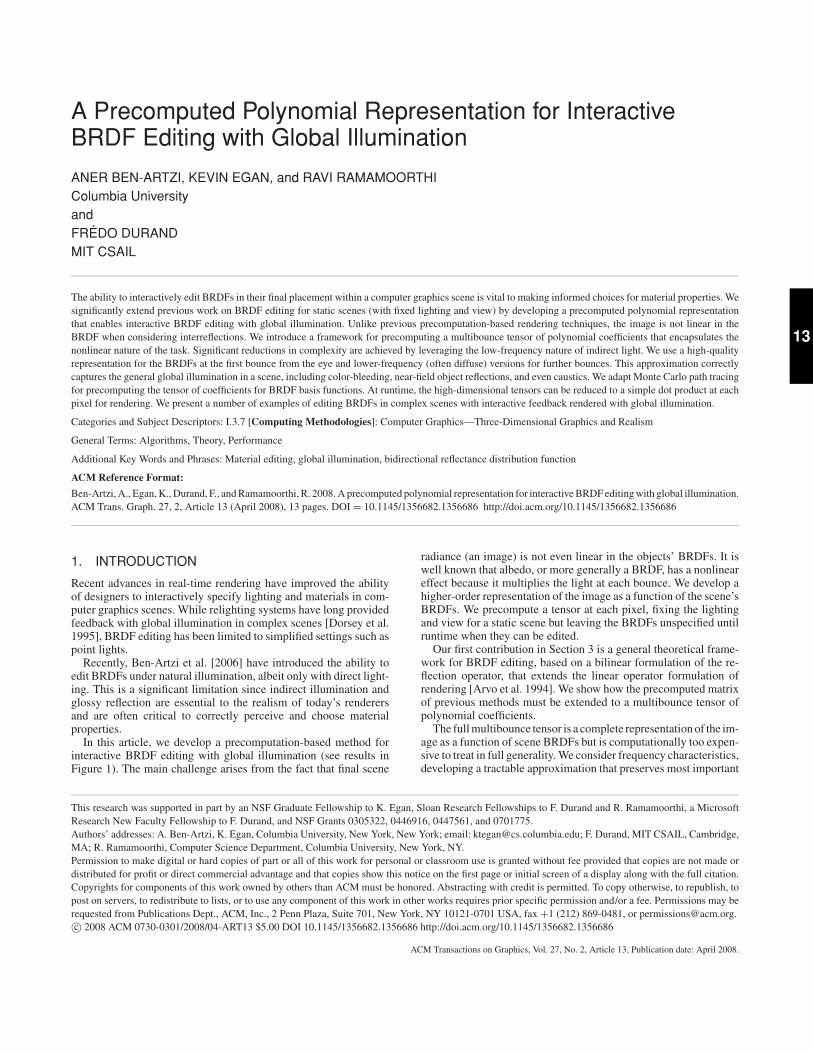
Fig. 1. We simulate an interior design session in which we edit the BRDFs of the couch and floor. The couch’s red fabric in (a) is loaded from measured

data and edited to a more specular green material in (b). The floor is retextured and made glossy in (b). The reflections of objects in the glossy floor and color

bleeding from the couch to the staircase can be seen here as well as in closeups in Figure 10. The scene is lit only from the large windows, using the top half

of an exterior environment map (campus). We can see in the comparisons to direct lighting (far right) that most of the room’s lighting is a result of indirect

illumination.

perceptual effects (Section 4). Specifically, the first bounce fromthe eye usually uses the full BRDF to capture glossy reflections,while subsequent bounces use a lower-frequency approximation tocapture overall shading effects. Within this general framework, weshow two possibilities: where further bounces (up to the fourth-bounce) are treated as purely diffuse (Figures 1, 6 and 9), and whereadditionally, the second bounce from the eye uses a lower-frequencyapproximation to achieve accurate indirect reflections in glossy sur-faces (Figure 4), or even intricate effects like caustics (Figure 11).

For precomputation (Section 5.1), we show how Monte Carlopath tracing can be extended to precompute the multibounce tensorsneeded. For rendering (Section 5.2), since only one object’s BRDFis edited at a time, we show that the tensor can be reduced to a fewvector dot products at each pixel whose coefficients can be computedin a very fast runtime preprocess. Our results show a variety of BRDFedits with interactive feedback rendered with global illumination.

2. PREVIOUS WORK

Precomputed Radiance Transfer (PRT). We build on PRTideas for static scenes [Sloan et al. 2002; Ng et al. 2003]. Whilethese methods focus on lighting design with fixed BRDFs, we focuson BRDF editing with fixed lighting. We are inspired by a body ofrecent work that underscores the importance of interreflections inrelighting [Hasan et al. 2006; Wang et al. 2006; Kontkanen et al.2006]. All these approaches exploit the linearity of relighting withrespect to light intensity, even when global illumination is takeninto account. In contrast, BRDF editing is fundamentally nonlinearwhen global illumination is considered.

Most previous PRT methods precompute a linear light transportvector at each image location, taking advantage of the linearity oflight. We extend this concept to a general tensor of coefficientsfor a high-dimensional polynomial. The idea of going from lin-ear to quadratic or cubic precomputed models has also begun tobe explored in physical simulation [Barbic and James 2005] but inthe context of differential equations and model dimensionality re-duction. In the context of real-time rendering, Sun and Mukherjee[2006] precompute with a larger product of functions, leading to anN -part multiplication at runtime. Each function is still precomputedindependently, and the runtime calculations are still linear in any ofthe individual functions.

While some PRT methods allow for all-frequency effects and viewchanges [Wang et al. 2006], BRDF editing cannot take advantage ofsuch factorization-based approaches since the BRDF lobe at a pixelis defined over both the dimensions of lighting (ωi ) and view (ωo)simultaneously and also depends on the surface normal. Therefore,we fix the lighting, view and geometry, but could, in principle, allowa small number of predefined views or lighting conditions to beupdated simultaneously (as in Ben-Artzi et al. [2006]).

Global Illumination. Our precomputation method is inspired byoffline global illumination algorithms such as Monte Carlo pathtracing [Kajiya 1986]. We have also been able to adapt finite elementradiosity [Cohen and Wallace 1993], although we found meshingand complexity issues difficult to deal with for our complex scenesand do not discuss it further. Global illumination techniques usuallyrequire the BRDF to be fixed, and use it for importance sampling orhierarchy construction. We develop extensions that are independentof the BRDF and allow real-time editing. In effect, we precomputea symbolic representation of the image, which can be evaluatedat runtime with polynomials in the user-specified BRDF values toobtain the final intensity.

Sequin and Smyrl [1989] also precompute a symbolic represen-tation of the final image for recursive ray tracing but not full globalillumination. Phong shading can be evaluated at runtime, allowinglater changes to surface parameters, while reflected and refractedcontributions are handled with pointers to subexpressions. In con-trast, we seek to simulate complex lighting and full global illumi-nation with many possible illumination paths. Therefore, we cannotafford to store or sum all subexpressions. Instead, we show that thefinal symbolic expression is a polynomial and only precompute itscoefficients. We also allow editing of general parametric and mea-sured BRDFs.

BRDF Representations and Editing. Recent work in BRDF edit-ing has begun to allow edits while rendering important visual effectssuch as environment maps [Colbert et al. 2006] and general complexlighting with cast shadows [Ben-Artzi et al. 2006]. However, theyare limited to direct lighting, which neglects many aspects of appear-ance in realistic settings with global illumination. We utilize existingBRDF representations, giving the user the ability to edit them in-teractively in a scene with complex lighting, shadows, and inter-reflections. Our method supports analytic models like Blinn-Phongor Cook-Torrance, measured half-angle distributions [Ashikhmin


A Precomputed Polynomial Representation for BRDF Editing with Global Illumination • 13:3

x x

x

xG K

B

BL

R

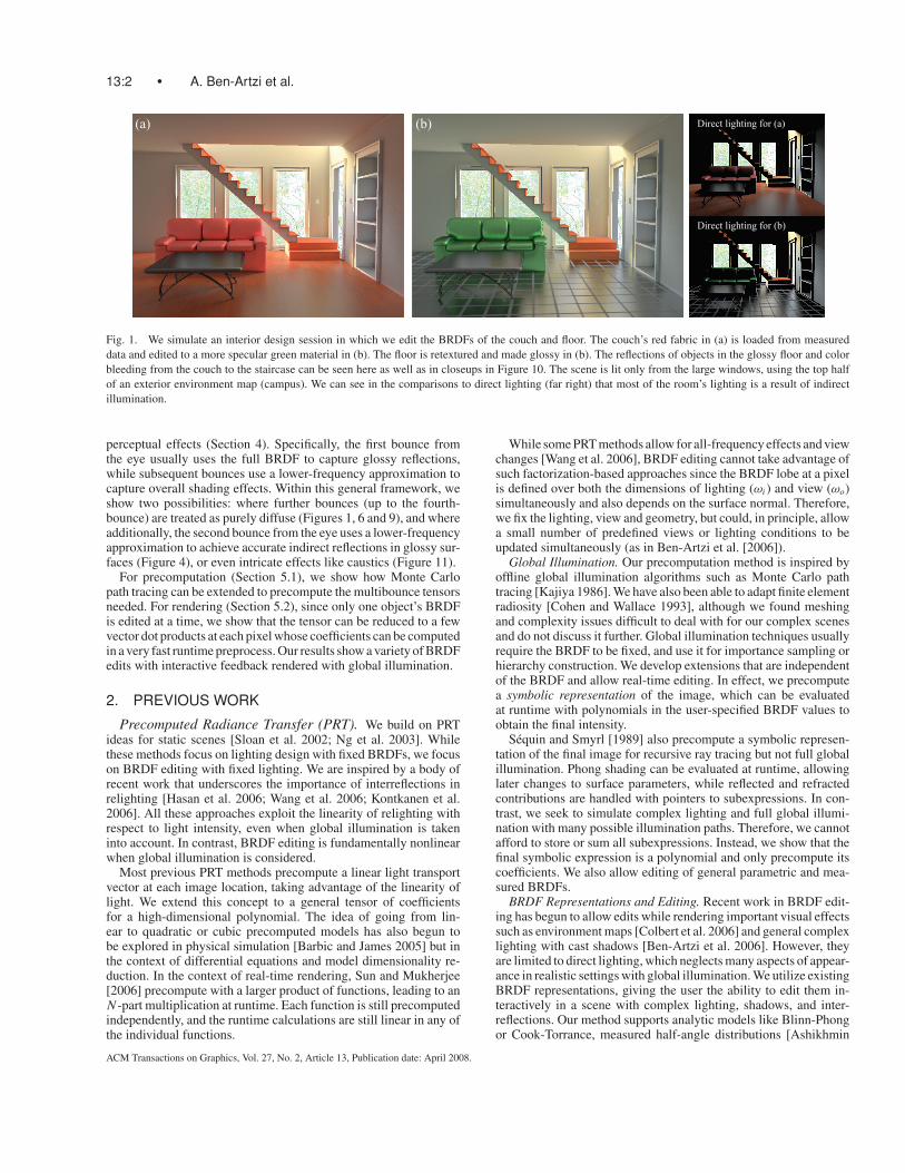
Fig. 2. Schematic of the rendering equation. Outgoing radiance from all

surfaces in the scene (left) is converted by the G operator into a local inci-

dent radiance field at each location (middle), which is then reflected via the

bilinear reflection operator K, that takes as input both the incident lighting

and the BRDF.

et al. 2000; Ngan et al. 2005], and variants of data-driven factoredor curve-based models [McCool et al. 2001; Lawrence et al. 2006].We allow users to either edit values corresponding to parameters instandard analytic BRDFs, or 1D curves for measured data.

Interactive Relighting with Dynamic BRDFs. In simultaneouswork Sun et al. [2007] have concurrently developed a precomputedapproach to interactive relighting with dynamic BRDFs. Both pa-pers observe that the image is nonlinear in the BRDF, a higher-order polynomial representation is needed for indirect light, andthat higher bounces can be computed with coarser representations.Sun et al. [2007] enable changing view by limiting themselves toonly two interreflection bounces and through the use of an in-outBRDF factorization that is accurate only for very low-frequencymaterials. Further approximations are used for glossy effects andindirect lighting. The BRDF space also needs to be specified in ad-vance to allow for a tensor decomposition. By contrast, we focus onvisually accurate results for BRDF editing. We are limited to fixedview and lighting, but by allowing greater flexibility in terms of theBRDFs (including very specular materials), we can represent andedit continuously. As seen in our results, we can also support threeor four bounce interreflections, including high-frequency causticeffects (Figure 11). Other significant contributions include the gen-eral theoretical framework for BRDF editing in Section 3, and thediscussion of complexity and low-frequency BRDF approximations(Section 4).

3. GENERAL THEORETICAL FRAMEWORK

This section introduces a general theoretical framework for BRDFediting with global illumination, independent of any specific im-plementation. It builds on the geometric and reflection operatorsintroduced by Arvo et al. [1994] and shows how BRDF editing canbe formulated in terms of a new bilinear reflection operator K. Theoperator notation is compact and alleviates the need for complex in-tegrals in the equations. In Section 4, we discuss our approximationswithin this framework that make the computation tractable.

3.1 Basic Framework Using the Bilinear K Operator

The rendering equation [Kajiya 1986] can be written as a linearoperator equation [Arvo et al. 1994]. We build on this foundationand write the rendering equation as:

B = E + K(R) GB, (1)

where B(x, ωo) is the outgoing surface radiance, E(x, ωo) is theemission, and G is the linear geometric operator that converts theoutgoing radiance from distant surfaces to a local incident radiancefield as in Arvo et al. [1994]. Figure 2 shows a schematic, and Table Isummarizes notation.

Table I. Table of Notation

B(x, ωo) Outgoing radiance (image)

E(x, ωo) Emissive radiance of light sources

L(x, ωi ) Local incident radiance

R(x, ωi , ωo) BRDFs of all points in the scene

T N (x, ωo) Precomputed multi-bounce tensor

ρm (ωi , ωo) BRDF of object mbm

j (ωi , ωo) Basis function j for the BRDF of object mHm (x) Spatial weight map or texture for object mG Linear geometric operator

G : B(x, ωo) �→ L(y, ωi )

(GB)(x, ω) ≡ B(x ′(x, ω), −ω)

K(R) Reflection operator (equation 2)

cmj BRDF coefficients (equation 4)

dm Equivalent albedo of object m (appendix B)

dz Product of albedos dm�Xi Light path with contribution f ( �Xi )

Fijn Tensor coefficient after freezing BRDFs

J Number of BRDF bases (usually 64 or 128)

M Number of objects (M ∼ 5)

W Total basis functions (W = J M ∼ 500)

Z Number of terms for diffuse dz (Z ∼ 64)

Arvo et al. [1994] define K as a linear reflection operator on thelocal incident radiance field L . In our first departure from previousrepresentations, we make explicit K’s dependence on the BRDFsR of scene objects. We write K as a bilinear operator that takes anadditional input R(x, ωi , ωo), which describes the BRDF at eachpoint in the scene and is the kernel of integration in K,

K : L(x, ωi ), R(x, ωi , ωo) �→ B(x, ωo)

(K(R) L)(x, ωo) ≡∫

�2π

R(x, ωi , ωo)L(x, ωi ) cos θi dωi . (2)

Note that K is bilinear or linear with respect to both inputs, inci-dent lighting L , and the BRDFs of objects in the scene R. That is,for scalars a and b,

K(a R1 + bR2) L = aK(R1) L + bK(R2) L

K(R) (aL1 + bL2) = aK(R) L1 + bK(R) L2. (3)

We now seek to relate R (and hence K) to editable BRDFs ofindividual objects. We assume there are M objects in the scene and,for now, that each object has a single BRDF. Let object m have1

BRDF ρm . We assume the BRDF can be represented as a linearcombination of functions over the domain (ωi , ωo),

ρm(ωi , ωo) =J∑

j=1

cmj bm

j (ωi , ωo). (4)

The BRDF basis functions b could be spherical harmonics, wavelets,or any other linear basis. We follow previous BRDF editing meth-ods [Ben-Artzi et al. 2006; Lawrence et al. 2006] that have usedbox functions over a suitable 1D parameterization such as the half-angle, as described in Appendix A. They have shown that a 1Dparameterization is appropriate for most BRDF edits as well as beingcompatible with parametric edits of most common BRDF models.

Our goal is to use these basis BRDFs to create a method that allowsus to alter the kernel of integration in the K operator by specifying

1We use superscripts to denote some property of the function and parentheses

for explicitly raising to a power, so ρ2 is the second in a series, whereas (ρ)2

is ρ-squared.



= c1

+ c2

+ c2c

1+ c

2c

2+ (c

1)2

+...c1c

2 +c1c

1+1 1 1 2 1 2 1 2 1 2 1

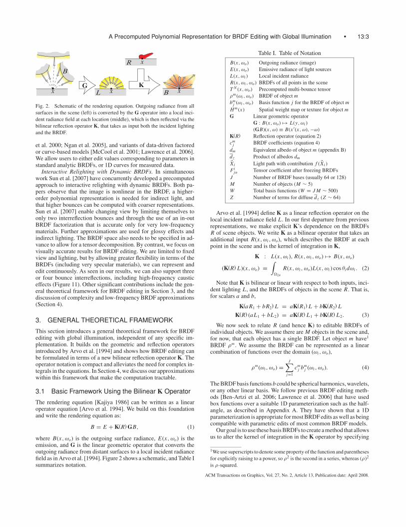
Fig. 3. The final value of each pixel is a polynomial in the BRDF coefficients. Here we show an example with 2 surfaces and 2 basis BRDFs shown in yellow

(diffuse and specular). Note that the BRDFs we use in practice are different. The combinatorics of multivariate polynomial coefficients make a tensor notation

particularly useful.

different weights cmj . We first need to use the bm

j s to describe Rover all surfaces. In order to encode per-object BRDFs, we define asurface mask H m(x) that is 1 if x is on object m, and 0 otherwise.2

R(x, ωi , ωo) =M∑

m=1

H mρm =M∑

m=1

H m(x)J∑

j=1

cmj bm

j (ωi , ωo) (5)

The super/subscripts in this equation implicitly define basis func-tions for the full spatially varying R,

R =M∑

m=1

J∑j=1

cmj Rm

j ; Rmj (x, ωi , ωo) = H m(x)bm

j (ωi , ωo). (6)

For simplicity, we will often use a single index w (or u or v) to referto the double script m

j , with w ∈ [1, W ] : W = M J .

3.2 Polynomial Representation for Multibounce

The solution of Equation (1) can be expressed as the expansion

B = E + K(R) GE + K(R) GK(R) GE + . . . , (7)

where each term N has an intuitive interpretation, as correspondingto N bounces of light from source(s) to viewer.

All current relighting methods rely on the linearity of B withrespect to E . Previous BRDF editing methods also take advantageof the linearity of the 1-bounce term in B (i.e., K(R) GE) withrespect to K (and hence with respect to R), requiring them to renderusing only direct lighting.

However, this linearity no longer applies for BRDF editing withglobal illumination because the operator K(R) is applied multipletimes. Even for 2-bounce reflections, the system becomes quadraticand must be represented with a quadratic multivariable polynomialin the cw s. The N -bounce solution is an order N polynomial. We nowshow how to extend the general PRT approach to these polynomialequations. We start by considering 2-bounce reflection,

B2 = K(R) GK(R) GE (8)

= K

(∑u

cu Ru

)GK

(∑v

cv Rv

)GE (9)

=∑

u

cu

(K(Ru) G

∑v

cv

(K(Rv) GE

))(10)

=∑

u

∑v

cucv K(Ru) GK(Rv) GE . (11)

The bilinear nature of K is crucial here. We use the linearity of Kwith respect to the BRDF to get Equation (10) and the linearity ofK and G with respect to radiance to get Equation (11).

2 H can also take on nonbinary values to encode spatial weight maps for

combining BRDFs [Lensch et al. 2001; Lawrence et al. 2006], and/or for

describing textures.

For BRDF editing, the coefficients (cu and cv ) become the vari-ables of our computation. The fixed quantities for precomputationare the basis BRDF distributions (Ru and Rv ) that depend only on theparameterizations of the various BRDFs. G and E are also known,defined by the geometry and lighting of the scene, respectively. Weprecompute a 2-bounce transport function T 2

uv and calculate B2 as

T 2uv = K(Ru) GK(Rv) GE

B2 =∑

u

∑v

T 2uv cucv . (12)

Most generally, T 2uv and B2 are defined over all spatial locations

and view directions. In practice, since we fix the view, T 2uv (x, ωo(x))

is an order 2 tensor (i.e., a matrix for 2-bounce reflection) at eachpixel. B2(x, ωo(x)) at each pixel is a quadratic polynomial in thevariables c, with coefficients given by T 2. When evaluated, it be-comes the radiance function for the scene due to light that has re-flected off exactly 2 surfaces. More explicitly,

B2 = T11(c1)2 + T12c1c2 + . . . Tuv cucv + . . . TW W (cW )2. (13)

Figure 3 illustrates such polynomials for paths of length 1 and 2.All 1- and 2-term combinations of the BRDFs are possible, includingrepetitions of the same basis function, as in T11(c1

1)2, since concaveobjects can reflect onto themselves. Following the same logic, theN -bounce energy is

B N =∑w N

∑w N−1

. . .∑w1

T Nw N w N−1 ...w1

cw N cw N−1. . . cw1

, (14)

where T N is an order N tensor for each pixel whose size varies withthe number of objects and BRDF basis functions per object. Weare evaluating a multivariable, degree N polynomial where each wruns over all W values (all basis functions). The variables of thispolynomial are the unknown scalar c’s. The coefficients are storedin T N ,

T Nw N w N−1···w1

= K(Rw N) GK

(Rw N−1

)G...K

(Rw1

)GE . (15)

Finally, we construct the image to be displayed by adding thecontributions from the different path-lengths:

B = E + B1 + B2 + · · · + B N , (16)

where we cut off the expansion in Equation (7) to N + 1 terms.

4. MANAGING COMPLEXITY

Section 3 has presented a theoretical framework that is fully gen-eral. However, we need to manage complexity in order to de-velop a tractable algorithm. In particular, the number of terms inEquation (14) is (W )N . Recall that W is already J M , the number ofbasis BRDFs times the number of objects. For typical values of M(5) and J (64–128), (so W ∼ 500) the computational and storage



)f)e)d)c)b)a

PBRT two bounces 128x8 bases 128x8 16x8 128x1 Direct

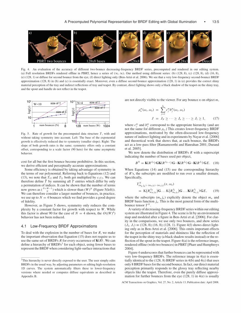
Fig. 4. An evaluation of the accuracy of different two-bounce decreasing-frequency BRDF series, precomputed and rendered in our editing system.

(a) Full resolution BRDFs rendered offline in PBRT, hence a series of (∞, ∞). Our method using different series: (b) (128, 8), (c) (128, 8), (d) (16, 8),

(e) (128, 1) or diffuse for second bounce from the eye, (f) direct lighting only (Ben-Artzi et al. 2006). We see that a very low-frequency second-bounce BRDF

approximation (128, 8) in (b) and (c) is essentially exact. Moreover, even a diffuse second-bounce approximation (128, 1) in (e) provides the correct shiny

material perception of the tray and indirect reflections of tray and teapot. By contrast, direct lighting shows only a black shadow of the teapot on the shiny tray,

and the spout and handle do not reflect in the teapot.

10

104

1 8

log(y

)

num bounces (N)

W=10

128 1024num bases (W)

log(y

)

N=4

10

1013size of T size of T

size of T~

size of T~

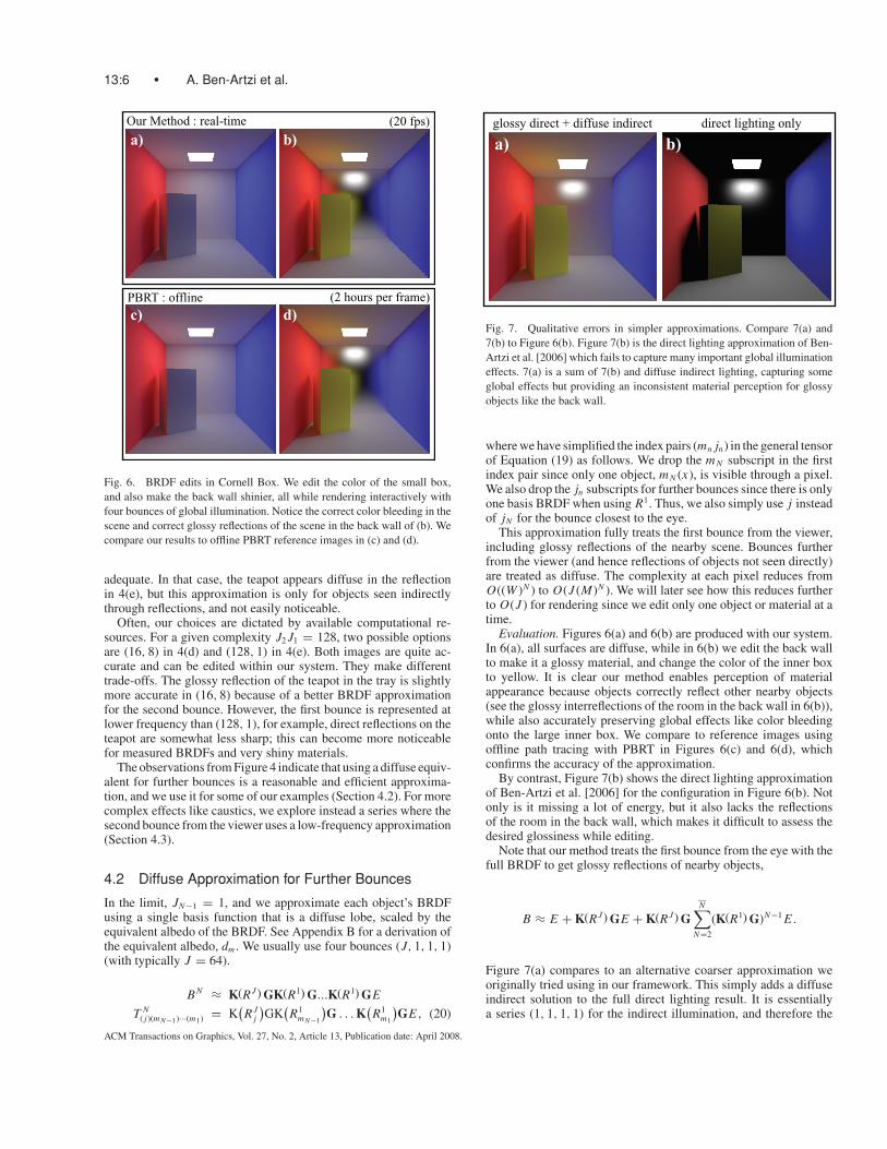
Fig. 5. Rate of growth for the precomputed data structure T , with and

without taking symmetry into account. Left: The base of the exponential

growth is effectively reduced due to symmetry (smaller slope). Right: The

slope of both growth rates is the same; symmetry offers only a constant

offset, corresponding to a scale factor (90 here) for the same asymptotic

behavior.

cost for all but the first bounce become prohibitive. In this section,we derive efficient and perceptually accurate approximations.

Some efficiency is obtained by taking advantage of symmetry inthe terms of our polynomial. Referring back to Equations (12) and(13), we note that T12 and T21 both get multiplied by c1c2. We cantherefore define T by summing all T entries which differ by onlya permutation of indices. It can be shown that the number of terms

now grows as ( N+W−1

N ) which is slower than (W )N (Figure 5(left)).We can therefore consider a larger number of bounces, in practice,we use up to N = 4 bounces which we find provides a good degreeof fidelity.

However, as Figure 5 shows, symmetry only reduces the com-plexity by a constant factor for growth with respect to W . Whilethis factor is about 90 for the case of N = 4 shown, the O((W )4)behavior has not been reduced.

4.1 Low-Frequency BRDF Approximations

To deal with the explosion in the number of bases for R, we makethe important observation that Equation (15) does not require us touse the same set of BRDFs R for every occurrence of K(R) . We candefine a hierarchy of BRDFs3 for each object, using fewer bases torepresent the BRDF when considering light-surface interactions that

3This hierarchy is never directly exposed to the user. The user simply edits

BRDFs in the usual way, by adjusting parameters or editing high-resolution

1D curves. The system automatically filters these to lower-frequency

versions where needed or computes diffuse equivalents as described in

Appendix B.

are not directly visible to the viewer. For any bounce n on object m,

ρmn (ωi , ωo) =

Jn∑j=1

cmj bm

j (ωi , ωo)

J = JN ≥ · · · ≥ Jn ≥ · · · ≥ J1 ≥ 1, (17)

where cmj and bm

j correspond to the appropriate hierarchy (and arenot the same for different ρn .) This creates lower-frequency BRDFapproximations, motivated by the often-discussed low-frequencynature of indirect lighting and in experiments by Nayar et al. [2006]and theoretical work that shows that, at each bounce, the BRDFsact as a low-pass filter [Ramamoorthi and Hanrahan 2001; Durandet al. 2005].

We now denote the distribution of BRDFs R with a superscriptindicating the number of bases used per object,

B N = K(R JN ) GK(R JN−1) G...K(R Jn) G...K(R J1) GE . (18)

When Equations (14) and (15) use the corresponding hierarchyof R’s, the subscripts are modified to run over a smaller domain.Specifically,

T N(mN jN )···(mn jn )···(m1 j1)(x, ωo)

= K(R JN

m N jN

)G . . . K

(R Jn

mn jn

)G . . . K(R J1

m1 j1) GE, (19)

where the subscripts (mn jn) explicitly denote the object mn andBRDF basis function jn . This is the most general form of the multi-bounce tensor T N .

A variety of decreasing-frequency BRDF series within our editingsystem are illustrated in Figure 4. The scene is lit by an environmentmap and modeled after a figure in Ben-Artzi et al. [2006]. For clar-ity in the comparisons, we use only two bounces, and show series(J2, J1) ≡ (128, 8); (16, 8); (128, 1). Figure 4(f) shows direct light-ing only as in Ben-Artzi et al. [2006]. This omits important effectsfor the perception of materials and shininess like the reflection ofthe teapot in the shiny tray (a black shadow results instead) or the re-flection of the spout in the teapot. Figure 4(a) is the reference image,rendered offline (with two bounces) in PBRT [Pharr and Humphreys2004].

Figure 4 underscores that further bounces can be represented withvery low-frequency BRDFs. The reference image in 4(a) is essen-tially identical to the (128, 8) BRDF series in 4(b) and 4(c) that usesonly 8 BRDF bases for the second bounce. In fact, our direct materialperception primarily responds to the glossy tray reflecting nearbyobjects like the teapot. Therefore, even the purely diffuse approxi-mation for further bounces from the eye (128, 1) in 4(e) is usually



Our Method : real-time

a)

c)

b)

d)PBRT : offline (2 hours per frame)

(20 fps)

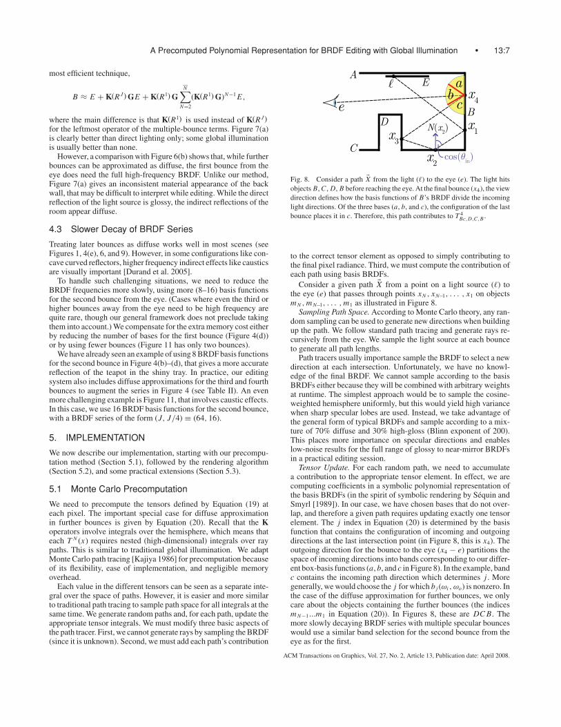
Fig. 6. BRDF edits in Cornell Box. We edit the color of the small box,

and also make the back wall shinier, all while rendering interactively with

four bounces of global illumination. Notice the correct color bleeding in the

scene and correct glossy reflections of the scene in the back wall of (b). We

compare our results to offline PBRT reference images in (c) and (d).

adequate. In that case, the teapot appears diffuse in the reflectionin 4(e), but this approximation is only for objects seen indirectlythrough reflections, and not easily noticeable.

Often, our choices are dictated by available computational re-sources. For a given complexity J2 J1 = 128, two possible optionsare (16, 8) in 4(d) and (128, 1) in 4(e). Both images are quite ac-curate and can be edited within our system. They make differenttrade-offs. The glossy reflection of the teapot in the tray is slightlymore accurate in (16, 8) because of a better BRDF approximationfor the second bounce. However, the first bounce is represented atlower frequency than (128, 1), for example, direct reflections on theteapot are somewhat less sharp; this can become more noticeablefor measured BRDFs and very shiny materials.

The observations from Figure 4 indicate that using a diffuse equiv-alent for further bounces is a reasonable and efficient approxima-tion, and we use it for some of our examples (Section 4.2). For morecomplex effects like caustics, we explore instead a series where thesecond bounce from the viewer uses a low-frequency approximation(Section 4.3).

4.2 Diffuse Approximation for Further Bounces

In the limit, JN−1 = 1, and we approximate each object’s BRDFusing a single basis function that is a diffuse lobe, scaled by theequivalent albedo of the BRDF. See Appendix B for a derivation ofthe equivalent albedo, dm . We usually use four bounces (J, 1, 1, 1)(with typically J = 64).

B N ≈ K(R J) GK(R1) G...K(R1) GE

T N( j)(m N−1)···(m1) = K

(R J

j

)GK

(R1

m N−1

)G . . . K

(R1

m1

)GE, (20)

direct lighting onlyglossy direct + diffuse indirect

a) b)

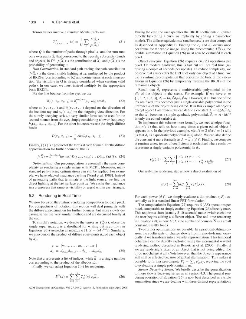
Fig. 7. Qualitative errors in simpler approximations. Compare 7(a) and

7(b) to Figure 6(b). Figure 7(b) is the direct lighting approximation of Ben-

Artzi et al. [2006] which fails to capture many important global illumination

effects. 7(a) is a sum of 7(b) and diffuse indirect lighting, capturing some

global effects but providing an inconsistent material perception for glossy

objects like the back wall.

where we have simplified the index pairs (mn jn) in the general tensorof Equation (19) as follows. We drop the m N subscript in the firstindex pair since only one object, m N (x), is visible through a pixel.We also drop the jn subscripts for further bounces since there is onlyone basis BRDF when using R1. Thus, we also simply use j insteadof jN for the bounce closest to the eye.

This approximation fully treats the first bounce from the viewer,including glossy reflections of the nearby scene. Bounces furtherfrom the viewer (and hence reflections of objects not seen directly)are treated as diffuse. The complexity at each pixel reduces fromO((W )N ) to O(J (M)N ). We will later see how this reduces furtherto O(J ) for rendering since we edit only one object or material at atime.

Evaluation. Figures 6(a) and 6(b) are produced with our system.In 6(a), all surfaces are diffuse, while in 6(b) we edit the back wallto make it a glossy material, and change the color of the inner boxto yellow. It is clear our method enables perception of materialappearance because objects correctly reflect other nearby objects(see the glossy interreflections of the room in the back wall in 6(b)),while also accurately preserving global effects like color bleedingonto the large inner box. We compare to reference images usingoffline path tracing with PBRT in Figures 6(c) and 6(d), whichconfirms the accuracy of the approximation.

By contrast, Figure 7(b) shows the direct lighting approximationof Ben-Artzi et al. [2006] for the configuration in Figure 6(b). Notonly is it missing a lot of energy, but it also lacks the reflectionsof the room in the back wall, which makes it difficult to assess thedesired glossiness while editing.

Note that our method treats the first bounce from the eye with thefull BRDF to get glossy reflections of nearby objects,

B ≈ E + K(R J) GE + K(R J) GN∑

N=2

(K(R1) G)N−1 E .

Figure 7(a) compares to an alternative coarser approximation weoriginally tried using in our framework. This simply adds a diffuseindirect solution to the full direct lighting result. It is essentiallya series (1, 1, 1, 1) for the indirect illumination, and therefore the



most efficient technique,

B ≈ E + K(R J) GE + K(R1) GN∑

N=2

(K(R1) G)N−1 E,

where the main difference is that K(R1) is used instead of K(R J)

for the leftmost operator of the multiple-bounce terms. Figure 7(a)is clearly better than direct lighting only; some global illuminationis usually better than none.

However, a comparison with Figure 6(b) shows that, while furtherbounces can be approximated as diffuse, the first bounce from theeye does need the full high-frequency BRDF. Unlike our method,Figure 7(a) gives an inconsistent material appearance of the backwall, that may be difficult to interpret while editing. While the directreflection of the light source is glossy, the indirect reflections of theroom appear diffuse.

4.3 Slower Decay of BRDF Series

Treating later bounces as diffuse works well in most scenes (seeFigures 1, 4(e), 6, and 9). However, in some configurations like con-cave curved reflectors, higher frequency indirect effects like causticsare visually important [Durand et al. 2005].

To handle such challenging situations, we need to reduce theBRDF frequencies more slowly, using more (8–16) basis functionsfor the second bounce from the eye. (Cases where even the third orhigher bounces away from the eye need to be high frequency arequite rare, though our general framework does not preclude takingthem into account.) We compensate for the extra memory cost eitherby reducing the number of bases for the first bounce (Figure 4(d))or by using fewer bounces (Figure 11 has only two bounces).

We have already seen an example of using 8 BRDF basis functionsfor the second bounce in Figure 4(b)–(d), that gives a more accuratereflection of the teapot in the shiny tray. In practice, our editingsystem also includes diffuse approximations for the third and fourthbounces to augment the series in Figure 4 (see Table II). An evenmore challenging example is Figure 11, that involves caustic effects.In this case, we use 16 BRDF basis functions for the second bounce,with a BRDF series of the form (J, J/4) ≡ (64, 16).

5. IMPLEMENTATION

We now describe our implementation, starting with our precompu-tation method (Section 5.1), followed by the rendering algorithm(Section 5.2), and some practical extensions (Section 5.3).

5.1 Monte Carlo Precomputation

We need to precompute the tensors defined by Equation (19) ateach pixel. The important special case for diffuse approximationin further bounces is given by Equation (20). Recall that the Koperators involve integrals over the hemisphere, which means thateach T N (x) requires nested (high-dimensional) integrals over raypaths. This is similar to traditional global illumination. We adaptMonte Carlo path tracing [Kajiya 1986] for precomputation becauseof its flexibility, ease of implementation, and negligible memoryoverhead.

Each value in the different tensors can be seen as a separate inte-gral over the space of paths. However, it is easier and more similarto traditional path tracing to sample path space for all integrals at thesame time. We generate random paths and, for each path, update theappropriate tensor integrals. We must modify three basic aspects ofthe path tracer. First, we cannot generate rays by sampling the BRDF(since it is unknown). Second, we must add each path’s contribution

Fig. 8. Consider a path �X from the light (�) to the eye (e). The light hits

objects B, C , D, B before reaching the eye. At the final bounce (x4), the view

direction defines how the basis functions of B’s BRDF divide the incoming

light directions. Of the three bases (a, b, and c), the configuration of the last

bounce places it in c. Therefore, this path contributes to T 4Bc,D,C,B .

to the correct tensor element as opposed to simply contributing tothe final pixel radiance. Third, we must compute the contribution ofeach path using basis BRDFs.

Consider a given path �X from a point on a light source (�) tothe eye (e) that passes through points xN , xN−1, . . . , x1 on objectsm N , m N−1, . . . , m1 as illustrated in Figure 8.

Sampling Path Space. According to Monte Carlo theory, any ran-dom sampling can be used to generate new directions when buildingup the path. We follow standard path tracing and generate rays re-cursively from the eye. We sample the light source at each bounceto generate all path lengths.

Path tracers usually importance sample the BRDF to select a newdirection at each intersection. Unfortunately, we have no knowl-edge of the final BRDF. We cannot sample according to the basisBRDFs either because they will be combined with arbitrary weightsat runtime. The simplest approach would be to sample the cosine-weighted hemisphere uniformly, but this would yield high variancewhen sharp specular lobes are used. Instead, we take advantage ofthe general form of typical BRDFs and sample according to a mix-ture of 70% diffuse and 30% high-gloss (Blinn exponent of 200).This places more importance on specular directions and enableslow-noise results for the full range of glossy to near-mirror BRDFsin a practical editing session.

Tensor Update. For each random path, we need to accumulatea contribution to the appropriate tensor element. In effect, we arecomputing coefficients in a symbolic polynomial representation ofthe basis BRDFs (in the spirit of symbolic rendering by Sequin andSmyrl [1989]). In our case, we have chosen bases that do not over-lap, and therefore a given path requires updating exactly one tensorelement. The j index in Equation (20) is determined by the basisfunction that contains the configuration of incoming and outgoingdirections at the last intersection point (in Figure 8, this is x4). Theoutgoing direction for the bounce to the eye (x4 − e) partitions thespace of incoming directions into bands corresponding to our differ-ent box-basis functions (a, b, and c in Figure 8). In the example, bandc contains the incoming path direction which determines j . Moregenerally, we would choose the j for which b j (ωi , ωo) is nonzero. Inthe case of the diffuse approximation for further bounces, we onlycare about the objects containing the further bounces (the indicesm N−1...m1 in Equation (20)). In Figures 8, these are DC B. Themore slowly decaying BRDF series with multiple specular bounceswould use a similar band selection for the second bounce from theeye as for the first.



Tensor values involve a standard Monte Carlo sum,

T Nw N w N−1 ...w1

(x) = 1

Q

∑i

f ( �Xi )

p( �Xi ), (21)

where Q is the number of paths through pixel x , and the sum runs

only over paths �Xi that correspond to the specific subscripts (bands

and objects) in T N . f ( �Xi ) is the contribution of �Xi , and p( �Xi ) is theprobability of generating it.

Path Contribution. In standard path tracing, the path contribution

f ( �Xi ) is the direct visible lighting at x1, multiplied by the productof BRDFs (corresponding to K) and cosine terms at each intersec-tion (the visibility in G is already considered when creating validpaths). In our case, we must instead multiply by the appropriatebasis BRDFs.

For the first bounce from the eye, we use

b j (e, xN , xN−1) = bm N (xN )j (ωi , ωo) cos θi , (22)

where ωi (xN , xN−1) and θi (xN , xN−1) depend on the direction ofthe incident ray and ωo(e, xN ) on the outgoing view direction. Forthe slowly decaying series, a very similar form can be used for thesecond bounce from the eye, simply considering a lower-frequencyb j (xN , xN−1, xN−2). For the other bounces, we use the single diffusebasis:

D(xn, xn−1) = 1

πcos(θi (xn, xn−1)). (23)

Finally, f ( �X ) is a product of the terms at each bounce. For the diffuseapproximation for further bounces, this is

f ( �X ) = bm N (xN )j (ωi , ωo)D(xN−1, xN−2) . . . D(x1, �)E(�). (24)

Optimizations. Our precomputation is essentially the same com-plexity as rendering a single image with MCPT. Moreover, manystandard path-tracing optimizations can still be applied. For exam-ple, we have adapted irradiance caching [Ward et al. 1988]. Insteadof generating paths that terminate at the light source, we find thedirect lighting at the last surface point x1. We cache the irradiancein a preprocess that samples visibility on a grid within each triangle.

5.2 Rendering in Real Time

We now focus on the runtime rendering computation for each pixel.For compactness of notation, this section will deal primarily withthe diffuse approximation for further bounces, but more slowly de-caying series use very similar methods and are discussed briefly atthe end.

To simplify notation, we denote the tensor as T Njz (x), where the

single super index z is a shorthand for writing out m N−1...m1 inEquation (20) (viewed as an index, z ∈ [1, Z = (M)N−1]). Similarly,we also denote the product of diffuse equivalents dm of each object

by dz ,

z ≡ {m N−1, . . . , mn, . . . , m1}dz ≡ dm N−1

dm N−2. . . dmn . . . dm2

dm1. (25)

Note that z represents a list of indices, while dz is a single numbercorresponding to the product of the albedos dm .

Finally, we can adapt Equation (14) for rendering,

B N (x) =J∑

j=1

Z∑z=1

T Njz (x) c j dz . (26)

During the edit, the user specifies the BRDF coefficients c j (eitherdirectly by editing a curve or implicitly by editing a parametric

model). The diffuse equivalents d (and hence dz) are then computed

as described in Appendix B. Finding the c j and dz occurs onceper frame for the whole image. Using the precomputed T N

jz (x), thedouble summation in Equation (26) must now be evaluated at eachpixel.

Object Freezing. Equation (26) requires O(J Z ) operations perpixel. On modern hardware, this is fast but still not real time (re-quiring a couple of seconds per update). To reduce complexity, weobserve that a user edits the BRDF of only one object at a time. Weuse a runtime precomputation that performs the bulk of the calcu-lations in Equation (26) by temporarily freezing the BRDFs of theremaining objects.

Recall that dz represents a multivariable polynomial in thed’s of the objects in the scene. For example, if we have z ={1, 3, 2, 1, 5, 3}, dz = (d1)2d2(d3)2d5. However, if all but one of thed’s are fixed, this becomes just a single-variable polynomial in theunfrozen d of the object being edited. If in this example all objectsexcept object 1 are frozen, we can define a constant A = d2(d3)2d5,

so that dz becomes a simple quadratic polynomial, dz = A · (d1)2

in only the edited variable d1.To implement this scheme more formally, we need a helper func-

tion n(z, i) that tells us how many times a given edited object iappears in z. In the previous example, n(z, i) = 2 (for i = 1) tells

us that dz is a quadratic polynomial in di alone. We can also define

the constant A more formally as A = dz/(di )n . Finally, we compute

at runtime a new tensor of coefficients at each pixel where each rowrepresents a single-variable polynomial in di ,

Fijn(x) =

∑N

∑z

{n(z, i) �= n : 0

n(z, i) = n : T Njz (x) dz

(di )n(27)

Our real-time rendering step is now a direct evaluation of

B(x) =N−1∑n=0

(di )n

J∑j=1

c j Fijn(x). (28)

For each power (di )n , we simply evaluate a dot-product c j Fj , es-

sentially as in a standard linear PRT formulation.The computation in Equation (27) requires O(J Z ) operations per

pixel, comparable to simply evaluating Equation (26) directly once.This requires a short (usually 5-10 seconds) mode switch each timethe user begins editing a different object. The real-time rendering

in Equation (28) is now O(J ) (the number of bounces N is a smallconstant, usually four.)

Two further optimizations are possible. In a practical editing ses-sion, the coefficients c j change slowly from frame-to-frame, espe-cially if we transform into a wavelet representation. This temporalcoherence can be directly exploited using the incremental waveletrendering method described in Ben-Artzi et al. [2006]. Finally, ifwe are rendering a pixel of an object that is not being edited, thec j do not change at all. (Note however, that the object’s appearancewill still be affected because of global illumination.) This makes itpossible to further precompute V i

n = ∑j Fi

jnc j , reducing the costto evaluating a simple polynomial in di .

Slower Decaying Series. We briefly describe the generalizationto more slowly decaying series as in Section 4.3. The general ren-dering operation of Equation (26) is now best described as a triplesummation since we are dealing with three distinct representations



of R: R JN , R JN−1 , and R1.

B N (x) =JN∑j=1

M JN−1∑w=1

Z∑z=1

T Njwz(x) c j cw dz, (29)

with cw denoting the lower-frequency BRDF coefficients for thesecond bounce (JN−1 bases on each of the M objects).

Object freezing is a bit more difficult, theoretically requiringthe creation of a three-dimensional Fi

jkn, where j ∈ [1, JN ],k ∈ [1, JN−1], n ∈ [0, N−2]. In practice, we think of the j asone dimension, and k ′ ≡ kn as the other.

5.3 Extensions

We briefly describe two important practical extensions.Objects with Fixed BRDFs. Large scenes can contain many small

objects that cause an exponential increase in memory requirements.Such scenes usually do not require editing the BRDFs of all objects.When designing the materials in a room, one typically does not wantto change the BRDFs of small placeholder objects like books ortoys. We extend our algorithm by implementing the ability to fix theBRDFs of certain objects at precomputation. Note that their shadingis still updated, based on global illumination from other surfaces.This should also not be confused with runtime object freezing, whichoccurs temporarily during an editing session.

In precomputation, instead of using diffuse equivalents D orBRDF bases b, we must use the full known BRDF ρm(ωi , ωo) cos θi

for reflections from fixed object m. Rendering is unchanged for ed-itable objects since there are no new BRDF bases. For the fixedobject, we still use T N

z (x) and multiply by the diffuse albedos ofeditable objects. However, the BRDF bases (and index j) need notbe considered. In Figure 1, the table and its legs have fixed BRDFs.

Spatial Weight Maps. So far, we have focused on BRDF effects.Spatial variation can be handled with textures to modulate the BRDFover an object’s surface. If we do not seek to edit them, the texturescan be directly incorporated into the BRDF basis functions (as themultiplicative H m(x) terms in Equation (5)). Finally, while we havediscussed a single BRDF per object for clarity, our framework andimplementation can handle multiple colocated BRDFs for each ob-ject. If we also seek to modify the spatial blending of BRDFs, aswe do for the floor in Figure 1, we can simply modulate the directlyviewed surfaces in image-space by the multiplicative spatial blend-ing weights (weight maps) or texture. For global illumination, weare concerned only with the low-frequency behavior of the weightmaps or textures, and we modulate the diffuse equivalent albedosby the average value of the weight map for each BRDF layer.

6. RESULTS

Section 6.1 briefly discusses the types of edit performed on thescenes in Figures 1, 4, 6, 9 and 11 and the global illumination ef-fects involved. Then, Section 6.2 gives performance results for pre-computation time and memory usage, while Section 6.3 discussesrendering frame rates.

6.1 Editing and Visual Effects

Cornell Box. Figure 6 shows the Cornell box where we edit theparameters of a Blinn-Phong and diffuse reflectance model. In go-ing from 6(a) to 6(b), we make the back wall glossy with correctinterreflections of the nearby scene and change the color of the in-ner box, demonstrating accurate color bleeding. Note that even the

)b)a

c)

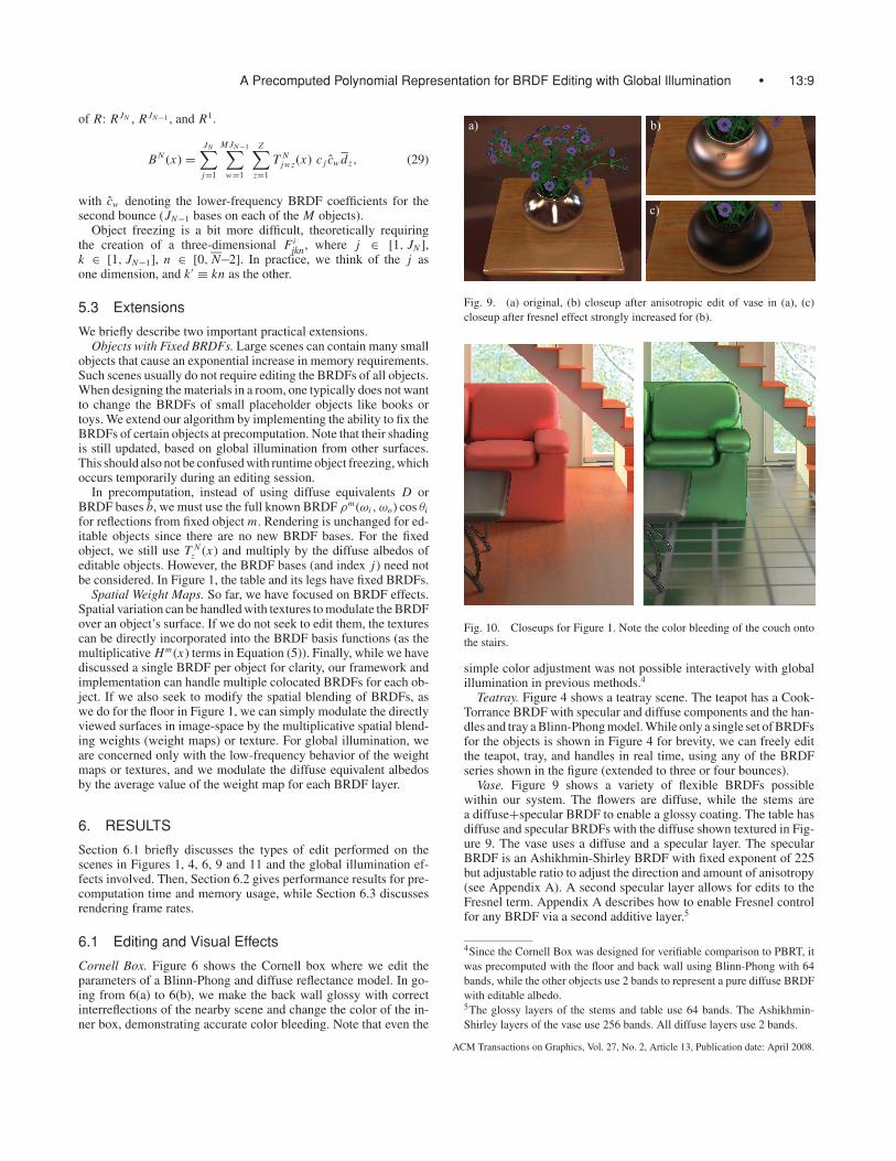
Fig. 9. (a) original, (b) closeup after anisotropic edit of vase in (a), (c)

closeup after fresnel effect strongly increased for (b).

Fig. 10. Closeups for Figure 1. Note the color bleeding of the couch onto

the stairs.

simple color adjustment was not possible interactively with globalillumination in previous methods.4

Teatray. Figure 4 shows a teatray scene. The teapot has a Cook-Torrance BRDF with specular and diffuse components and the han-dles and tray a Blinn-Phong model. While only a single set of BRDFsfor the objects is shown in Figure 4 for brevity, we can freely editthe teapot, tray, and handles in real time, using any of the BRDFseries shown in the figure (extended to three or four bounces).

Vase. Figure 9 shows a variety of flexible BRDFs possiblewithin our system. The flowers are diffuse, while the stems area diffuse+specular BRDF to enable a glossy coating. The table hasdiffuse and specular BRDFs with the diffuse shown textured in Fig-ure 9. The vase uses a diffuse and a specular layer. The specularBRDF is an Ashikhmin-Shirley BRDF with fixed exponent of 225but adjustable ratio to adjust the direction and amount of anisotropy(see Appendix A). A second specular layer allows for edits to theFresnel term. Appendix A describes how to enable Fresnel controlfor any BRDF via a second additive layer.5

4Since the Cornell Box was designed for verifiable comparison to PBRT, it

was precomputed with the floor and back wall using Blinn-Phong with 64

bands, while the other objects use 2 bands to represent a pure diffuse BRDF

with editable albedo.5The glossy layers of the stems and table use 64 bands. The Ashikhmin-

Shirley layers of the vase use 256 bands. All diffuse layers use 2 bands.



low glossring:

high gloss

diffuseground plane:

high glosslow gloss

medium gloss

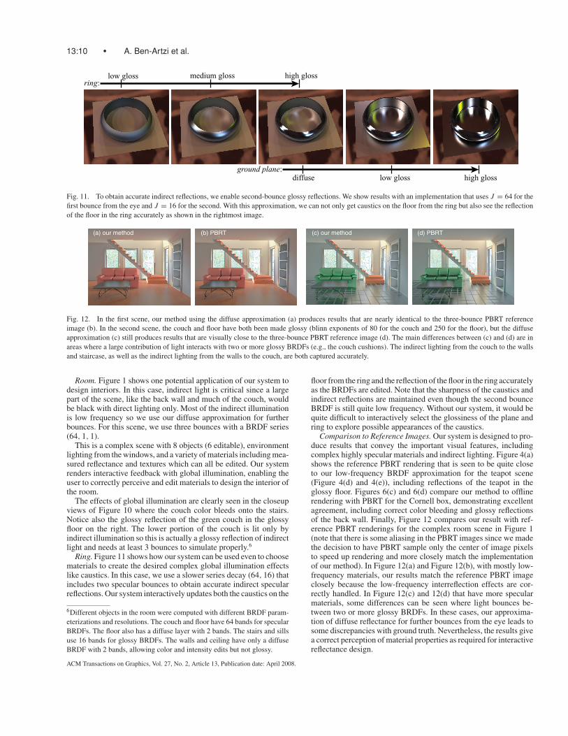
Fig. 11. To obtain accurate indirect reflections, we enable second-bounce glossy reflections. We show results with an implementation that uses J = 64 for the

first bounce from the eye and J = 16 for the second. With this approximation, we can not only get caustics on the floor from the ring but also see the reflection

of the floor in the ring accurately as shown in the rightmost image.

(a) our method (c) our method(b) PBRT (d) PBRT

Fig. 12. In the first scene, our method using the diffuse approximation (a) produces results that are nearly identical to the three-bounce PBRT reference

image (b). In the second scene, the couch and floor have both been made glossy (blinn exponents of 80 for the couch and 250 for the floor), but the diffuse

approximation (c) still produces results that are visually close to the three-bounce PBRT reference image (d). The main differences between (c) and (d) are in

areas where a large contribution of light interacts with two or more glossy BRDFs (e.g., the couch cushions). The indirect lighting from the couch to the walls

and staircase, as well as the indirect lighting from the walls to the couch, are both captured accurately.

Room. Figure 1 shows one potential application of our system todesign interiors. In this case, indirect light is critical since a largepart of the scene, like the back wall and much of the couch, wouldbe black with direct lighting only. Most of the indirect illuminationis low frequency so we use our diffuse approximation for furtherbounces. For this scene, we use three bounces with a BRDF series(64, 1, 1).

This is a complex scene with 8 objects (6 editable), environmentlighting from the windows, and a variety of materials including mea-sured reflectance and textures which can all be edited. Our systemrenders interactive feedback with global illumination, enabling theuser to correctly perceive and edit materials to design the interior ofthe room.

The effects of global illumination are clearly seen in the closeupviews of Figure 10 where the couch color bleeds onto the stairs.Notice also the glossy reflection of the green couch in the glossyfloor on the right. The lower portion of the couch is lit only byindirect illumination so this is actually a glossy reflection of indirectlight and needs at least 3 bounces to simulate properly.6

Ring. Figure 11 shows how our system can be used even to choosematerials to create the desired complex global illumination effectslike caustics. In this case, we use a slower series decay (64, 16) thatincludes two specular bounces to obtain accurate indirect specularreflections. Our system interactively updates both the caustics on the

6Different objects in the room were computed with different BRDF param-

eterizations and resolutions. The couch and floor have 64 bands for specular

BRDFs. The floor also has a diffuse layer with 2 bands. The stairs and sills

use 16 bands for glossy BRDFs. The walls and ceiling have only a diffuse

BRDF with 2 bands, allowing color and intensity edits but not glossy.

floor from the ring and the reflection of the floor in the ring accuratelyas the BRDFs are edited. Note that the sharpness of the caustics andindirect reflections are maintained even though the second bounceBRDF is still quite low frequency. Without our system, it would bequite difficult to interactively select the glossiness of the plane andring to explore possible appearances of the caustics.

Comparison to Reference Images. Our system is designed to pro-duce results that convey the important visual features, includingcomplex highly specular materials and indirect lighting. Figure 4(a)shows the reference PBRT rendering that is seen to be quite closeto our low-frequency BRDF approximation for the teapot scene(Figure 4(d) and 4(e)), including reflections of the teapot in theglossy floor. Figures 6(c) and 6(d) compare our method to offlinerendering with PBRT for the Cornell box, demonstrating excellentagreement, including correct color bleeding and glossy reflectionsof the back wall. Finally, Figure 12 compares our result with ref-erence PBRT renderings for the complex room scene in Figure 1(note that there is some aliasing in the PBRT images since we madethe decision to have PBRT sample only the center of image pixelsto speed up rendering and more closely match the implementationof our method). In Figure 12(a) and Figure 12(b), with mostly low-frequency materials, our results match the reference PBRT imageclosely because the low-frequency interreflection effects are cor-rectly handled. In Figure 12(c) and 12(d) that have more specularmaterials, some differences can be seen where light bounces be-tween two or more glossy BRDFs. In these cases, our approxima-tion of diffuse reflectance for further bounces from the eye leads tosome discrepancies with ground truth. Nevertheless, the results givea correct perception of material properties as required for interactivereflectance design.



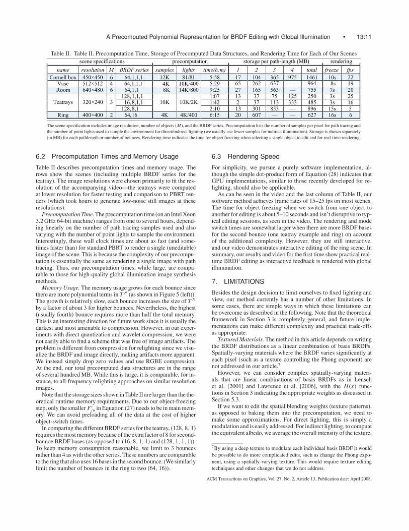
Table II. Table II. Precomputation Time, Storage of Precomputed Data Structures, and Rendering Time for Each of Our Scenes scene specifications precomputation storage per path-length (MB) rendering

name resolution M BRDF series samples lights time(h:m) 1 2 3 4 total freeze fps Cornell box 450×450 6 64,1,1,1 12K

4K81/81 5:58 17

65104262

365637

975 1461964

10s8s

2219Vase 512×512 4 64,1,1,1

Room 640×480 6 64,1,1 8K 14K/80010K/400

9:255:29

27 165 563 ——

755 7s 20 52 s3 052 521 57 73 31 70:1 1,1,1,821 61 s3 584 333 311 73 2 24:1 1,1,8,61Teatrays 320×240 3

128,8,1 10K 10K/2K

2:10 13 301 853 — 896 15s 5 Ring 400×400 2 64,16 4K 4K/400 6:15 20 607 — — 627 16s 6

,

,

,

The scene specification includes image resolution, number of objects (M), and the BRDF series. Precomputation lists the number of samples per pixel for path tracing and

the number of point lights used to sample the environment for direct/indirect lighting (we usually use fewer samples for indirect illumination). Storage is shown separately

(in MB) for each pathlength or number of bounces. Rendering time indicates the time for object freezing when selecting a single object to edit and for real-time rendering.

6.2 Precomputation Times and Memory Usage

Table II describes precomputation times and memory usage. Therows show the scenes (including multiple BRDF series for theteatray). The image resolutions were chosen primarily to fit the res-olution of the accompanying video—the teatrays were computedat lower resolution for faster testing and comparison to PBRT ren-ders (which took hours to generate low-noise still images at theseresolutions).

Precomputation Time. The precomputation time (on an Intel Xeon3.2 GHz 64-bit machine) ranges from one to several hours, depend-ing linearly on the number of path tracing samples used and alsovarying with the number of point lights to sample the environment.Interestingly, these wall clock times are about as fast (and some-times faster than) for standard PBRT to render a single (uneditable)image of the scene. This is because the complexity of our precompu-tation is essentially the same as rendering a single image with pathtracing. Thus, our precomputation times, while large, are compa-rable to those for high-quality global illumination image synthesismethods.

Memory Usage. The memory usage grows for each bounce sincethere are more polynomial terms in T N (as shown in Figure 5 (left)).The growth is relatively slow, each bounce increases the size of T N

by a factor of about 3 for higher bounces. Nevertheless, the highest(usually fourth) bounce requires more than half the total memory.This is an interesting direction for future work since it is usually thedarkest and most amenable to compression. However, in our exper-iments with direct quantization and wavelet compression, we werenot easily able to find a scheme that was free of image artifacts. Theproblem is different from compression for relighting since we visu-alize the BRDF and image directly, making artifacts more apparent.We instead simply drop zero values and use RGBE compression.At the end, our total precomputed data structures are in the rangeof several hundred MB. While this is large, it is comparable, for in-stance, to all-frequency relighting approaches on similar resolutionimages.

Note that the storage sizes shown in Table II are larger than the the-oretical runtime memory requirements. Due to our object-freezingstep, only the smaller Fi

jn in Equation (27) needs to be in main mem-ory. We can avoid preloading all of the data at the cost of higherobject-switch times.

In comparing the different BRDF series for the teatray, (128, 8, 1)requires the most memory because of the extra factor of 8 for second-bounce BRDF bases (as opposed to (16, 8, 1, 1) and (128, 1, 1, 1)).To keep memory consumption reasonable, we limit to 3 bouncesrather than 4 as with the other series. These numbers are comparableto the ring that also uses 16 bases in the second bounce. (We similarlylimit the number of bounces in the ring to two (64, 16)).

6.3 Rendering Speed

For simplicity, we pursue a purely software implementation, al-though the simple dot-product form of Equation (28) indicates thatGPU implementations, similar to those recently developed for re-lighting, should also be applicable.

As can be seen in the video and the last column of Table II, oursoftware method achieves frame rates of 15–25 fps on most scenes.The time for object-freezing when we switch from one object toanother for editing is about 5–10 seconds and isn’t disruptive to typ-ical editing sessions, as seen in the video. The rendering and modeswitch times are somewhat larger when there are more BRDF basesfor the second bounce (one teatray example and ring) on accountof the additional complexity. However, they are still interactive,and our video demonstrates interactive editing of the ring scene. Insummary, our results and video for the first time show practical real-time BRDF editing as interactive feedback is rendered with globalillumination.

7. LIMITATIONS

Besides the design decision to limit ourselves to fixed lighting andview, our method currently has a number of other limitations. Insome cases, there are simple ways in which these limitations canbe overcome as described in the following. Note that the theoreticalframework in Section 3 is completely general, and future imple-mentations can make different complexity and practical trade-offsas appropriate.

Textured Materials. The method in this article depends on writingthe BRDF distributions as a linear combination of basis BRDFs.Spatially-varying materials where the BRDF varies significantly ateach pixel (such as a texture controlling the Phong exponent) arenot addressed in our article.7

However, we can consider complex spatially-varying materi-als that are linear combinations of basis BRDFs as in Lenschet al. [2001] and Lawrence et al. [2006], with the H (x) func-tions in Section 3 indicating the appropriate weights as discussed inSection 5.3.

If we want to edit the spatial blending weights (texture patterns),as opposed to baking them into the precomputation, we need tomake some approximations. For direct lighting, this is simply amodulation and is easily addressed. For indirect lighting, to computethe equivalent albedo, we average the overall intensity of the texture.

7By using a deep texture to modulate each individual basis BRDF it would

be possible to do more complicated edits, such as change the Phong expo-

nent, using a spatially-varying texture. This would require texture editing

techniques and other changes that we do not address.



This does have the limitation that the surface would appear uniformand untextured as seen in the reflection on a nearby glossy object.Nevertheless, our system allows textures to contribute for the firstbounce and average albedo to material perception. In Figure 1, weload in different spatial weight maps (textures) for the room’s floorto demonstrate runtime texture changes.

Scalability. The nature of global illumination requires accountingfor an increasing number of events for higher bounces. This com-plexity, and our techniques for dealing with it, are discussed in detailin Section 4. One consequence is that our method is currently notscalable to scenes with tens to hundreds of objects, where each hasan editable BRDF. We can get around this by using fixed BRDFs forsmall objects that need not be edited as discussed in Section 5.3. Inthe more general case, however, an iterative approach would needto be employed. The user needs to edit a few materials at a time(such as a single couch and table), followed by a new precomputa-tion to enable edits to other objects, while fixing the BRDFs of thematerials already edited.

Complex BRDFs. A general editing system should be able tohandle almost any analytic or measured BRDF. In practice, mem-ory and computation limit us to 1D functions of a given BRDFparameterization (often the half-angle). Nevertheless, our represen-tation does capture the full 4D-nature of the BRDF. Appendix Adescribes the most general form amenable to editing within oursystem. As described in Ben-Artzi et al. [2006] and recapped inAppendix A, the quotient BRDF can be arbitrarily complex. It isonly the editable behavior that must be describable as a function ofsome 1D-parameterization. Figure 9 shows a single material (thevase) for which we edit both the direction of anisotropy, and thenthe Fresnel effect, always rendering with the Geometric AttenuationFactor as part of the BRDF model.

Sampling Noise and Banding Artifacts. The specific implemen-tation choices for our precomputation may, in some cases, lead tobanding and sampling artifacts. Both the environment and area lightsare sampled with static point samples. This is an implementationchoice made in the ray tracer for precomputation and not a limita-tion of our approach. Environment map samples were chosen with amethod similar to Agarwal et al. [2003]. This is the largest contrib-utor to the banding artifacts, which are most noticeable when usingmaterials that are near-mirror.

For indirect lighting, we sample, as described in Section 5.1, with70% diffuse and 30% Blinn exponent 200. While this greatly reducesthe noise for most materials, near-mirrors still show some noise. Wenote that near-mirrors are the ultimate stress test for our system sincethey effectively promote each of the light bounces by 1. However,we still handle them rather well, and, in other realistic materials,these effects are much less noticeable. Note that the quality of theimages can be chosen by the user, depending only on the CPU timeallocated to the preprocess. (Indeed, some previous precomputation-based methods have allocated 100’s of CPU hours to produce veryhigh-quality images.)

8. CONCLUSIONS AND FUTURE WORK

This article has described a complete theoretical analysis and practi-cal implementation of a real-time rendering method, which enablesinteractive editing of BRDFs with global illumination effects. Weexpect that our method will have significant applications to designin computer graphics where the artist can now interactively specifymaterial properties in the final scene with complex lighting, shadowsand interreflections.

In the process, we develop a new precomputation-based frame-work that can handle nonlinear effects involving multivariable poly-

nomials for multiple bounces. Our contributions include a gen-eral theoretical framework for expressing global illumination as aprecomputation-based interactive rendering process based on reflec-tion and geometric operators, an analysis of computational complex-ity to develop tractable approximations, and effective precomputa-tion and rendering methods and extensions. It is likely that many ofthese insights could be used in other contexts, like PRT for relight-ing, or even offline global illumination.

More generally, we have proposed a new and efficient method forsymbolically rendering an image. Instead of accumulating each pathin the color of a single pixel, that path is effectively stored in sym-bolic form, including the product of all BRDF terms encounteredalong it. Paths involving the same BRDF terms are accumulated inthe appropriate tensor coefficient. This symbolic approach is likelyto have broad applications in other domains where we seek to in-teractively edit or explore the space of material parameters, such asanimation, simulation, and geometric modeling.

APPENDIXES

Appendix A: BRDF Basis Functions

Our framework is general for any choice of linear BRDF basis func-tions but benefits from those tailored to the natural space in whichmaterial edits occur. In practice, we use the 1D-reparameterizedbox basis functions of Ben-Artzi et al. [2006],

ρ(ωi , ωo) = ρq (ωi , ωo) f (γ ); f =J∑j

c j b j (γ (ωi , ωo)), (30)

where f is the 1D-editable factor, and ρq is the quotient BRDF thatcaptures more complex but uneditable behavior like normalizationconstants and the GAF . f can be set directly by the user by editinga 1D-curve or computed by the system based on the user settingparameters of analytic BRDFs. The previous form involves an ap-propriate 1D-parameterization γ of the BRDF’s 4D-domain. Someexamples of γ are: θhalf, θdiff, θin, and θout.

Some BRDFs have two factors such as Cook Torrance withγ = θhalf to control specular behavior and γ = θdiff to controlthe Fresnel effect. We use only a single factor for practical reasons,to keep memory requirements manageable. However, we show inthe following that many of the important two-curve edits can beachieved with a single factor, by careful use of the quotient BRDF.

The Fresnel effect is the most common use of the θdi f f factor. Ifwe use the Schlick [1994] approximation, a BRDF that includes aFresnel term (e.g. Cook-Torrance) becomes

ρ = ρq f (θh)(F + (1 − F)(1 − cos θd )5). (31)

F is a function of the wavelength (color channel) and index ofrefraction only. This allows us to define ρ as the sum of two BRDFs,each with just one editable factor but different ρq ,

ρ = ρq f1 + ρq2f2; f1 = F f (θh)

ρq2= (1 − cos θd )5ρq ; f2 = (1 − F) f (θh) (32)

At runtime, F is evaluated based on the user’s choice of index ofrefraction, and f1 and f2 are set via the user interface. The twoBRDFs are computed and summed (just as a specular and diffuselayer would be summed) to yield an accurate composite.

Anisotropy is the result of an elongated highlight. As presented inBen-Artzi et al. [2006], two factors can be used to adjust the widthof the highlight along the tangent and binormal directions. If weknow the overall specularity of the material, we can separate theAshikhmin-Shirley BRDF into a quotient that captures the width of



the highlight and a 1D-factor that controls the ratio of the elongationin the two perpendicular directions:

ρAS = ρq (cos θh)nu cos φh (cos θh)(rnu ) sin φh ; r ≡ nv/nu (33)

ρAS = ρqu(ωi , ωo)(γr (ωh, ωo))r (34)

γr = (cos θh)nu sin φh ; ρqu = ρq (cos θh)nu cos φh (35)

A similar single-factor form can be obtained if the amount and di-rection of anisotropy (r ) is known and only the width of the highlightneeds to be adjusted.

Appendix B: Equivalent Albedo

We choose the equivalent albedo to match the average BRDF value,or more exactly, the output power for a uniform incident radiancefield. This also corresponds formally to choosing the best perturbedK operator as in Arvo et al. [1994]. In other words,

d = 1

π

∫ ∫ρ(ωi , ωo) cos θi cos θo dωi dωo

= 1

π

∑j

c j

∫ ∫ρq (ωi , ωo)b j (γ (ωi , ωo)) cos θi cos θo dωi , dωo.

(36)

The term in the integral now depends only on known quantities—the quotient BRDFs and the basis functions, and can therefore beevaluated by dense Monte Carlo sampling (this needs to be doneonly once for a given parameterization, not even for each scene).Call this e j . Finally, at runtime, we simply need to compute

d = 1

π

∑j

c j e j , (37)

with the predetermined e j and the dynamically chosen c j .

ACKNOWLEDGMENTS

We thank Charles Han for his help in setting up the testing frame-work. Jonathan Ragan-Kelley, Jan Kautz and Nicolas Holzschuchread early drafts of this article, making many valuable suggestions,as did the anonymous reviewers.

REFERENCES

AGARWAL, S., RAMAMOORTHI, R., BELONGIE, S., AND JENSEN, H. 2003.

Structured importance sampling of environment maps. ACM Trans.Graph. (SIGGRAPH’03) 22, 3.

ARVO, J., TORRANCE, K., AND SMITS, B. 1994. A framework for the

analysis of error in global illumination algorithms. In SIGGRAPH’94,

75–84.

ASHIKHMIN, M., PREMOZE, S., AND SHIRLEY, P. 2000. A mirofacet-based

BRDF generator. In SIGGRAPH’00, 65–74.

BARBIC, J., AND JAMES, D. 2005. Real-time subspace integration of

St. Venant-Kirchoff deformable models. ACM Trans. Graph. (SIG-GRAPH’05) 24, 3, 982–990.

BEN-ARTZI, A., OVERBECK, R., AND RAMAMOORTHI, R. 2006. Real-

time BRDF editing in complex lighting. ACM Trans. Graph. (SIG-GRAPH’06) 25, 3, 945–954.

COHEN, M., AND WALLACE, J. 1993. Radiosity and Realistic ImageSynthesis. Academic Press.

COLBERT, M., PATTANAIK, S., AND KRIVNEK, J. 2006. Brdf-shop: Cre-

ating physically correct bidirectional reflectance distribution functions.

IEEE Comput. Graph. Appl. 26, 1.

DORSEY, J., ARVO, J., AND GREENBERG, D. 1995. Interactive design

of complex time dependent lighting. IEEE Comput. Graph. Appl. 15, 2

(March), 26–36.

DURAND, F., HOLZSCHUCH, N., SOLER, C., CHAN, E., AND SILLION, F. X.

2005. A frequency analysis of light transport. ACM Trans. Graph.(SIGGRAPH’05) 24, 3, 1115–1126.

HASAN, M., PELLACINI, F., AND BALA, K. 2006. Direct to indirect trans-

fer for cinematic relighting. ACM Trans. Graph. (SIGGRAPH’06) 25, 3,

1089–1097.

KAJIYA, J. 1986. The rendering equation. In SIGGRAPH’86.

KONTKANEN, J., TURQUIN, E., HOLZSCHUCH, N., AND SILLION, F. 2006.

Wavelet radiance transport for real-time indirect lighting. In Proceedingsof the EuroGraphics Symposium on Rendering.

LAWRENCE, J., BEN-ARTZI, A., DECORO, C., MATUSIK, W., PFISTER, H., RA-

MAMOORTHI, R., AND RUSINKIEWICZ, S. 2006. Inverse shade trees for

non-parametric material representation and editing. ACM Trans. Graph.25, 3, 735–745.

LENSCH, H. P. A., KAUTZ, J., GOESELE, M., HEIDRICH, W., AND SEIDEL, H.-

P. 2001. Image-based reconstruction of spatially varying materials.

In 12th Eurographics Workshop on Rendering, 103–114.

MCCOOL, M., ANG, J., AND AHMAD, A. 2001. Homomorphic factor-

ization of BRDFs for high-performance rendering. In SIGGRAPH ’01,

171–178.

NAYAR, S., KRISHNAN, G., GROSSBERG, M., AND RASKAR, R. 2006. Fast

separation of direct and global components of a scene using high frequency

illumination. ACM Trans. Graph. (SIGGRAPH’06) 25, 3, 935–944.

NG, R., RAMAMOORTHI, R., AND HANRAHAN, P. 2003. All-frequency

shadows using non-linear wavelet lighting approximation. ACM Trans.Graph. (SIGGRAPH’03) 22, 3, 376–381.

NGAN, A., DURAND, F., AND MATUSIK, W. 2005. Experimental analysis

of BRDF models. In Proceedings of the Europe Graphics Symposium onRandom, 117–126.

PHARR, M., AND HUMPHREYS, G. 2004. Physically Based Rendering:From Theory to Implementation. Morgan Kaufmann.

RAMAMOORTHI, R., AND HANRAHAN, P. 2001. A signal-processing

framework for inverse rendering. In SIGGRAPH’01, 117–128.

SCHLICK, C. 1994. An inexpensive BRDF model for physically-based

rendering. Comput. Graph. For. 13, 3, 233–246.

SEQUIN, C. H., AND SMYRL, E. K. 1989. Parameterized ray tracing. In

SIGGRAPH’89, vol. 23.

SLOAN, P., KAUTZ, J., AND SNYDER, J. 2002. Precomputed radiance

transfer for real-time rendering in dynamic, low-frequency lighting envi-

ronments. ACM Trans. Graph. (SIGGRAPH’02) 21, 3.

SUN, W., AND MUKHERJEE, A. 2006. Generalized wavelet product in-

tegral for rendering dynamic glossy objects. ACM Trans. Graph. (SIG-GRAPH’06) 25, 3, 477–487.

SUN, X., ZHOU, K., CHEN, Y., LIN, S., SHI, J., AND GUO, B. 2007. In-

teractive relighting with dynamic BRDFs. ACM Trans. Graph. (SIG-GRAPH’07) 26, 3, 27.

WANG, R., TRAN, J., AND LUEBKE, D. 2006. All-frequency relighting of

glossy objects. ACM Trans. Graph. 25, 2, 293–318.

WARD, G., RUBINSTEIN, F., AND CLEAR, R. 1988. A ray tracing solution

for diffuse interreflection. In SIGGRAPH’88, 85–92.

Received July 2007; accepted November 2007


A Precomputed Polynomial Representation for …ravir/brdfgi.pdfA Precomputed Polynomial...

Documents

Transcript of A Precomputed Polynomial Representation for …ravir/brdfgi.pdfA Precomputed Polynomial...