1

Polygon Vertex Set Matching Algorithm for Shapefile Tweening

Razvan Corneliu Carbunescu

Department of Computer Science

University of California at Berkeley

carazvan@eecs.berkeley.edu

Sarah Van Wart

School of Information

University of California at Berkeley

vanwars@ischool.berkeley.edu

Abstract This paper will explore the potential for a generalized

animation library and user interface scheme to facilitate

the understanding of geospatial datasets as they change

over time. By creating an easy way to (1) load, annotate,

and interact with shapefiles (a proprietary GIS format

developed by ESRI), (2) animate and morph complex

polygons across shapefiles in a time series, and (3)

integrate this functionality with popular mapping APIs

(such as Modest Maps and Google Maps), a GIS

visualization framework can be created to assist users in

identifying patterns and trends in spatio-temporal data. At

the root of this problem is the need to find a good way to

match polygons across shapefiles, and to solve the Polygon

Vertex Matching problem, one of the most important

underlying problems of creating visual changes between

sets of polygons in a display. There currently does not exist

any good way of presenting the changes of two areas

represented in shapefiles because of the very complex

nature of the polygons that fail most matching criteria of

current algorithms. As a result morphing shapes (tweening)

Figure 1 User interface enables shapefile tweening, allows for layer visibility interaction, and provides basic pan and zoom functionality.

Figure 2 Tween of a representative sample polygon

is reduced in most visualization packages to simple tweens

between regular well known shapes like triangles or

squares and is currently simply used in visualizing scatter

plots or similar displays. Visual morphing or tweening

would be of great importance in understanding changes in

physical areas that are represented by complex polygons in

shapefiles. In addition to a proposed Flash-based UI, this

paper presents an algorithm that achieves a good vertex

matching between sets of polygons without making

serious assumptions about the properties of said shapes

and that reduces vertex matching artifacts.

Introduction

Shapefiles and GIS Software

Shapefiles [1] currently represent the most ubiquitous

format used to store, retrieve and visualize map data and

spatial features. Large collections of shapefiles exist in a

variety of data arenas and can store spatial and attribute

data about political, economic, ecological, transportation,

and parcel information, among other things. Though these

shapefiles represent spatial information as a snapshot in

time, many of these shapefiles exist among a collection of

other similar shapefiles corresponding to a different date

as part of a time series (weekly, monthly, yearly). In this

scenario, it makes sense for GIS technologies to provide a

way in which to visually represent these changes over

time, given that the most important properties of shapefile

records are the shapes of the actual regions themselves.

Ott and Swiaczny note in their book on Time-Integrative

GIS that “a crucial motivation for the development of time-

integrative GIS techniques is the fact that enormous

amounts of data have been collected in the last decades by

census offices, research projects, and not the least

companies, which can be revaluated and reused” and that

there are not simple ways to visually display “the forest

boundaries between 1850 and 1950” [2]. Simply

observing the overlap of regions between two shapefiles

can make it difficult to interpret shape differences

between the overlaid polygons, and if more than two

shapefiles are considered the transitions become nearly

impossible to understand or represent. Many GIS experts

hold that "animation can be used as an exploratory tool to

detect similarities or differences in distribution within a

series of maps. This is especially possible when one can

interactively access the individual frames in an animation

and quickly switch between individual maps or map

sequences [3]."

Tweening

Tweening, an important tool in the field of visualization, is

the process by which one image is transformed into

another image by generating intermediate frames

between the two to give the appearance of a smooth

transition. While the concept of animation is not by any

means new to visualization, techniques for the animating

of more complicated shapes – those for which no simple,

underlying structure (table, tree, scatter plot, etc.) exists –

have not been well developed. Polygon tweening is one of

the remaining problems to be solved efficiently and

correctly for complicated shapes. Some complex morphing

capabilities exist in the newest version of Flash, but these

capabilities rely upon ‘hints’ given by the programmer, and

do not work well for polygons with large vertex, which are

typical in shapefiles.

Related Work Existing Spatio-Temporal Data Visualizations

From the GIS perspective, a number of GIS applications

have been built with some capacity for GIS animation.

Perhaps the closest of these is TimeMap, which has

separate Java-based and Flash-based web map viewers

that support spatio-temporal sense-making. The Flash-

based viewer can animate GIS files by tweening vector

polygons, but exploratory tasks currently must be done in

a separate Java-based viewer where data is animated by

playing a number of successive frames which toggle

features on and off according to a date filter. The GeoTime

time-space visualization framework allows users to

interactively create their own event-based stories over

time and animate them on demand, but in this case the

events are point-based and do not provide for smooth

transitions between polygons. ESRI also has several

desktop-based applications and plug-ins such as Arc Hydro

and STARS that allow for basic animation of geospatial

data. Regarding the ability to easily view shapefiles on the

web, Edwin van Rijkom wrote a simple library to import

shapefiles into Flash.

Existing Vertex Set Matching Algorithms

There exist a good number of polygon vertex set matching

algorithms in the literature but it seems that every one

3

comes with very stringent requirements on the type of

polygons it can handle, or with exceptions that cannot be

easily handled by shapefile polygons. Some interesting

algorithms on this topic are:

Morphing using Extended Gaussian Image [4] converts a

convex polygon into its Extended Gaussian Image (EGI) and

then uses this representation on both images to construct

the intermediate values. The algorithm first computes the

ECI of the source and of the target polygons. Next it

matches source and target normals on the ECI circle

creating source-target normal pairs. Then it linearly

interpolates weights and angles between normal pairs to

derive the ECI of intermediate steps. Finally, it reconstructs

the convex polygon corresponding to the ECI obtained by

interpolating the normals. This algorithm works well but

only for convex polygons whose EGI is unique. Most

shapefile polygons are unfortunately far from convex.

Line length and inner angle interpolation [5] method uses

the representation of the polygon as a set of lines and

inner angles and simply linearly interpolates between this

set for the initial polygon and the final polygon. While this

approach has the advantage of being inherently simple and

fast the choosing of the correct vertices when the polygon

vertex number doesn’t match between the initial and final

polygon make this method not applicable towards

shapefile polygons as these are unlikely to ever match if

the polygon shape has changed.

Triangulation Algorithms [6] transform the polygon into a

set of triangles with a skeleton link and then changes the

triangulation from one set to another by minimizing

‘physical force’ required to move triangles from the initial

configuration to the final. These algorithms are perhaps

the most promising for the purpose of guaranteeing no

fake intersections or topological changes in the

intermediate polygons. The problem with this algorithm

though is the particular requirement for ‘compatible

polygons’, namely creating a common graph of the centers

of both polygon triangulations with the same linking

structure which is not. The Steiner tree problem also that

it uses to find the final link between triangles is an NP-

complete problem so an approximation of the Steiner tree

must be calculated. The algorithm would create much

more movement in the matching to keep parts connected

and non-intersecting. Still this approach would present the

best alternative algorithm for generating polygon matching

especially since it has the ability to best represent texture

and texture morphing on the polygons should this feature

be desired.

Methodology

Domain and Data Selection

We decided to explore one of the many scenarios in which

smooth-transition polygon morphing could be applied to a

visualization problem – changes in land-use over time.

Though we realized that the way in which land-use evolves

doesn’t necessarily follow a smooth pattern of linear

growth, the movement of the edges of certain polygons

would be a much strong visual cue of geographic change

that simply turning each data layer on and off and

requiring the use to make the determination based on

iterative comparisons. We found a time-series, geospatial

dataset for land use in Hillsborough County, Florida that

consisted of a series of shapefiles that had been

generated for 1999, 2004, 2005, and 2006 from aerial

photography. These files were downloaded from the

Southwest Florida Water Management District’s public

access website and re-projected from the FL Albers

coordinate system into WGS84 using ArcGIS desktop

software from ESRI. Since the dataset was quite large, only

a subset of the land-use data – those polygons associated

with farmlands for a small area of the county – was

ultimately used, as a proof of concept.

User Interface

We decided to build the application infrastructure on top

of Flash, Flex, and Flare, because of the robust support

that Flash has for vector graphics, animation, and creating

smooth transitions between shapes. Several pre-existing

technologies were integrated together to create a mapping

interface for the land use shapefiles. We used a pre-

existing Flash library created by Edwin van Rijkom to parse

and display shapefile polygons in a Flex application. To

give these shapefile polygons some context, we decided to

use the Modest Maps API to support map tiling, panning,

and zooming. Each of the polygon shapefile layers was

symbolized, and a section was added to enable users to

turn the layers on and off so that they could manually

compare the differences in land use across the given years.

Finally, upon map initialization, the four shapefiles were

pre-loaded into the Flex application from the file system

and cached in memory for quick retrieval. Though this

technique would not work for large sets of shapefiles, it

worked for our purposes as a proof of concept.

Polygon Matching Algorithm

Initially, we naively assumed that it would be possible to

use some sort of unique polygon attribute to match

polygons from one temporal snapshot to another. That is,

we had hoped that a polygon from the 1999 land use

shapefile could be mapped to a polygon in the 2004

shapefile using some sort of unique identifier. In reality,

we found that typically no such historical continuity is

explicitly recorded across spatio-temporal GIS snapshots

(for a number of reasons), so we had to use methods for

approximating polygon intersection. Since we wanted to

focus primarily on the actual polygon morphing problem,

we developed a simple algorithm for mapping overlapping

polygons to each other by:

(1) Calculating the areas and centroids of each

polygon, P1 and P2.

(2) Calculating a “polygon radius,” based on the area

such that:

𝑅1 = 𝐴1

𝜋 , 𝑅2 =

𝐴2

𝜋

(3) Calculating the distance between the two polygon

centroids:

𝐷 = 𝑥2 − 𝑥1 2 + 𝑦2 − 𝑦1

2

(4) Asserting that if D < R1 + R2, then the polygons

intersect

Figure 3 Centroid & Radius Matching (match if D < R1 + R2)

Using this method, we iterated through each shapefile, and

matched each polygon to a preceding polygon and a

succeeding polygon if intersection was determined. We

stored this matching information in a data structure in

memory so that it could be accessed quickly for the

animation routine.

Vertex Set Matching Algorithm

The first step in matching two polygons is finding the

minimum distance between a vertex on the initial polygon

and a second vertex on the second polygon. This first step

is one of the most important assumptions in this algorithm

as a bad match here can result in very bad behavior in the

match. Most polygons presented though will satisfy this

property that the closest pair of points between any two

points will represent a correct matching. Usually this can

be thought of as the part of the polygon that stays

unchanged or the part of the polygon that moves the least.

After this pair is found, since the vertex list for both

polygons can be thought of as a circular linked list, the

vertices are reordered with the new pair of vertices being

the first element in either polygon. This matching gives the

algorithm a reference point from which to check for edge

intersections at the level of the vertices assigned in the

assignment problem step.

Next another simple step is taken in finding the second

minimum distance between two vertices with this second

matching used to create an initial line from which

distances can then be calculated by the vertex alignment

part. The selection of this second minimum vertex is also a

delicate task as it has a major influence over the rest of the

code. However unlike the first step this second matching

can be at some point changed during the course of the

algorithm which is not true for the initial matching.

With these two pairs of vertices and the list in the

reordered fashion a distance matrix between all pairs of

points is calculated. The appropriate changes are made to

the original distance matrix received to simulate the value

of the matrix after the assignment problem algorithm

would have selected those vertices. The steps are

subtracting the value of the matching distance m(k0,l0)

from all the first row where k0 is the first vertex in the

reorganized first polygon and l0 is the first vertex in the

reorganized second polygon. The other step is similar only

it involves creating the row and column values of the

assignment problem for imin2, jmin2 and subtracting this from

the matrix.

The main part of the vertex set algorithm now starts,

which runs the normal assignment algorithm with the

5

same steps in changing the matrix for each iteration but

with the following major changes:

In order to preserve edge order if x is the truth assignment

matrix:

∀ 𝑖, 𝑗, 𝑘, 𝑙 𝑠. 𝑡. 𝑖, 𝑗 ∈ 𝑉𝑃𝑜𝑙𝑦𝑔𝑜𝑛 1

𝑘, 𝑙 ∈ 𝑉𝑃𝑜𝑙𝑦𝑔𝑜𝑛 2

𝑡𝑕𝑒𝑛 𝑖𝑓

𝑖 < 𝑗𝑥𝑖 ,𝑘 = 1

𝑥𝑗 .𝑙 = 1 ,

→ 𝑘 < 𝑙

What this means, if we are looking at the matrix x, is that

given any matching at row i at position k, there can be no

matching in a row j unless it matches with a higher column

number l. This condition imposes a limit on how far to the

left or right a column j can look to improve a value in the

assignment problem. This also imposes a limit on the initial

population of the minimum distance to a column since not

all free rows can reach all columns. This limitation also

brings an important question as to whether the algorithm

will ever finish since there is a possibility that no

improvement can be done but in this case the algorithm

sees that no change has been done and produces a

temporary output from the non-matched vertex creation

part of the algorithm. The only true property other than

the algorithm that is kept from the assignment problem is

that at the level of the assignment matrix no vertex is

allowed to be matched with more than one other vertex.

𝑥 =

1 ⋯⋮ ⋱

0⋮

⋯ ⋯⋯ ⋯

0 ⋯ 1 ⋯ 0⋯ ⋯⋯ ⋯

⋮0

⋱ ⋯⋯ ⋱

Figure 4 Positions for assignment values given a 1 at position (i,j)

(green – valid; red – invalid)

Given a partial assignment matrix we check whether we

can run the vertex creation algorithm, namely whether all

current non-matched vertices are lying along an edge on

the matching. This means that there exists no pair i,j for

which the matching skips both the line i and the column j.

If the partial assignment matrix doesn’t check out then we

proceed to the next step. Mathematically the test for the

vertex creation part can be expressed as:

∄ 𝑖, 𝑗 𝑠. 𝑡. 𝑏𝑜𝑡𝑕

𝑥𝑖 ,𝑘 = 0

𝑛𝑐−1

𝑘=0

𝑥𝑘 ,𝑗 = 0

𝑛𝑟−1

𝑘=0

The vertex creation algorithm creates two new temporary

lists for each polygon. The algorithm adds both first

vertices to the new temporary lists and starts in the top-

left corner (position 0,0) of the assignment matrix and

works its way down from the i,j position where xi,j =1

towards the nr-1,nC-1 position by the following pattern(we

treat the array as if there existed xnr , nc =1 ):

Matching a point to an edge happens by selecting the

closest point on the edge to the point we want to match.

The method for doing this is calculating the perpendicular

point that crosses the line of the edge and then depending

on which side of the segment it falls into (outside or inside

the segment) selecting one of the endpoints of the

segment or the actual perpendicular distance to the point.

Figure 5 Matching a point to a segment (point – gray dot, segment –

blue line, NewP – orange dot

From these two temporary vertex arrays we can calculate

an approximate sum or value of how good our

approximation is by simply taking the distance between

matching i-i pairs of points. Because of the construction of

the temporary arrays they have the same number of

points, that the matching is i to i, and all points are in

order.

𝑠𝑢𝑚𝑐𝑢𝑟𝑒𝑛𝑡 𝑠𝑡𝑒𝑝

= 𝑉𝑡𝑚𝑝𝑖1𝑥− 𝑉𝑡𝑚𝑝𝑖

2𝑥

2+ 𝑉𝑡𝑚𝑝𝑖

1𝑦− 𝑉𝑡𝑚𝑝𝑖

2𝑦

2𝑛𝑛𝑒𝑤

𝑖=0

The final part of the algorithm is at every step of adding

another part to the assignment checking whether the

current sum is worse than the previous sum case in which

we stop. We also check that we have not reached the

number of vertices of one of the polygons.

Algorithm speed is approximately O(n3) worst case

scenario (where n = min(n1,n2) but matching needs to be

run only once at load time of shapefiles so calculating time

may be hidden. Algorithm performs well when one of the

n1 is small < 300 regardless in majority to the size of n2.

The algorithm slows significantly when presented with

matching two extremely large polygons n1, n2 > 1000. For

this case in particular a special part was added to the

algorithm to specify the maximum time that it can spend

trying to match two polygons. If the algorithm reaches that

time and still has not found ‘best’ solution the algorithm

gives the last previous temporary stored array which

represents the best approximation at the time of the

matching.

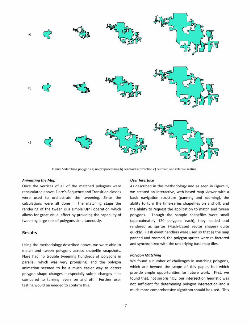
Algorithm Preprocessing of Polygons

By inspection on the normal types of polygons that were

asked to be matched certain pre-algorithm changes to the

program appeared to work very well in helping the

algorithm give a good match in most cases:

Figures that suffer translation in the physical image can

provide very bad initial data should vertices from opposite

sides overlap because of the transition. Also in most cases

position of the object should not affect how it changes its

shape so the first pre-processing option is subtracting the

centroid values of both polygon at the start of the

algorithm and adding them back after the matching has

happened. This will center both polygons on the same spot

to better allow for matching.

In the same way that translation can be partially taken out

of the equation of matching by subtracting the centroid of

the polygon, another important part of preprocessing is

relative scaling (scaling the polygon by a factor of the ratio

of areas of the two polygons). This procedure will make

both polygons be the ‘same size’ and will allow for a much

better match in general. In the code the relative scaling

can only be turned on when selecting centroid removal

also because scaling would bring some questions of what

point remains the same (the top-left corner of the

bounding box, the centroid of object, etc.). In the Relative

Scaling case with centroid removal the scaling location is

well defined and does not need to choose any options.

Since the preprocessing mentioned above isn’t always the best approximation, all three possible versions are computed (no preprocessing, centroid subtraction only, centroid and relative scaling) and the best distance between groups of given vertices is kept as the best solution. The general percentages of success between the three procedures seem to be 10% no preprocessing, 10% centroid subtraction and 80% centroid and relative scaling in selecting the best solution. This suggests that a simple acceleration of the algorithm with the penalty of correctness might be to simply run all polygons with the option of centroid and relative scaling.

7

Animating the Map

Once the vertices of all of the matched polygons were

recalculated above, Flare’s Sequence and Transition classes

were used to orchestrate the tweening. Since the

calculations were all done in the matching stage the

rendering of the tween is a simple O(n) operation which

allows for great visual effect by providing the capability of

tweening large sets of polygons simultaneously.

Results

Using the methodology described above, we were able to

match and tween polygons across shapefile snapshots.

Flare had no trouble tweening hundreds of polygons in

parallel, which was very promising, and the polygon

animation seemed to be a much easier way to detect

polygon shape changes – especially subtle changes – as

compared to turning layers on and off. Further user

testing would be needed to confirm this.

User Interface

As described in the methodology and as seen in Figure 1,

we created an interactive, web-based map viewer with a

basic navigation structure (panning and zooming), the

ability to turn the time-series shapefiles on and off, and

the ability to request the application to match and tween

polygons. Though the sample shapefiles were small

(approximately 120 polygons each), they loaded and

rendered as sprites (Flash-based vector shapes) quite

quickly. Flash event handlers were used so that as the map

panned and zoomed, the polygon sprites were re-factored

and synchronized with the underlying base map tiles.

Polygon Matching

We found a number of challenges in matching polygons,

which are beyond the scope of this paper, but which

provide ample opportunities for future work. First, we

found that, not surprisingly, our intersection heuristic was

not sufficient for determining polygon intersection and a

much more comprehensive algorithm should be used. This

a)

b)

c)

Figure 6 Matching polygons a) no preprocessing b) centroid subtraction c) centroid and relative scaling

became apparent when we observed that polygons were

actually tweening to adjacent, rather than overlapping

polygons from the subsequent Shapefile in the time series.

One way in which this could be addressed would be to

incorporate the polygon union and intersection functions

that are part of the open-source Java library, JTS [7].

Another issue that we noticed was that a one-to-one

polygon matching algorithm was overly simplistic. There

are in fact cases where an animation would be better

characterized by splitting a source polygon and having it

tween to several destination polygons, for example in the

event that a section of land is bisected by a new roadway.

Similarly, there are cases where several source polygons

should tween to a single destination polygon, for example

if several parcels of land were incorporated into a larger

area. Hence, many-to-many polygon matching support

should be incorporated into the library.

Vertex Set Matching

The polygons that were processed and tweened from the

shapefiles varied in sizes and shapes, so we were able to

gain a fairly wide range of the possible polygon tweening

scenarios with which the procedure had to contend.

There were some performance issues when matching one

large polygon (over 3,000 vertices) to another large

polygon, and a strategy would be needed to address

certain Flash timeout errors that occurred when processing

large geometries. The algorithm implementation itself,

however, was quite successful in creating smooth, natural

transitions between polygons. We observed various

shapes in order to determine ‘errors’ in the morphing.

Note that while the algorithm guarantees that there will

not be any edge crossing in the initial step of assignment,

in the non-matched vertex problem this assumption can be

broken. Below is a set of polygon tweens implemented

with the algorithm described in the paper which all

presented different challenges:

Figure 7 Sample results a) tweening a hole into a polygon b) matching 7(5:2)-7(2:5) vertex polygons produces 10 vertex polygons c) matching a test polygon with a real polygon

a)

b)

c)

9

Discussion

The matching algorithm discussed in this paper has been

implemented as a class object in the Flare Visualization

toolkit [8]. The data is read in from the shapefile using a

modified version of the Van Rijkom libraries [9] for

shapefiles. The class was created to extend previous

existing classes in order to allow for other tweens like

color, rotation, and even embedding to be done as simply

as using another common shape like a rectangle or circle.

From this proof of concept, it seems feasible – through (1)

improved polygon matching heuristics, (2) a batch-

processing of vertex matching between large polygons,

and (3) some indexing strategy to handle large shapefiles –

to have a generic framework by which shapefiles can be

animated across temporal snapshots in a generic manner.

These animations, in conjunction with addition

visualization tools, will greatly improve the way in which

spatio-temporal datasets can be explored.

Future Work

Tweening Enhancements

While the algorithm to morph simple polygons to other

polygons was completed, much of the theory that was

thought of for this project initially never managed to get it

to the code so a short description of the rest of the

algorithms that were developed will follow now and will

end with algorithms that need to be developed for better

tweening but that were not thought of during the time of

the class project:

Tweening polygons which contain holes represent are a

surprisingly important part of shapefile tweening, as

almost all polygons have some hole or another. The

algorithm to render the holes already exists in the code

and consists of rendering the entire object in one single

pass but by creating ‘cuts’ that reach the holes. The

algorithm for the holes would start by matching the outer

polygon shape to final polygon. The holes would then be

‘moved’ to the final position by weighted distance sum

with closest vertices getting weight based on the inverse of

the distance to a point. We would find the matching

between holes in final polygon by simple polygon matching

algorithm (the centroid radius approach described in the

paper). We create an initial adding of the holes into the

representation of the polygon by means of the special cuts.

While there are still holes not matched we find the closest

centroid to an edge and connect the centroid (the

intersection with the edge of the hole) to the edge of the

outer polygon and then repeat making sure to now

consider the hole as part of the ‘outer’ polygon. This

algorithm is O(h2

n) where h is the number of holes and the

n is the number of vertices on the outer polygon. Finally

we match the connecting cuts to the final polygon again by

weighted distance sum.

Tweening many to many polygons will probably represent

the final step in a polygon matching algorithm as this

would depend on all other parts working and itself

recursively narrowing the number in the groups of

polygons that need to be matched. We match the convex

hulls of the groups of polygons one to another. The convex

hull around the group of ‘initial’ polygons creates a ‘hole’

the inside of which represents the empty space between

the all polygons. This ‘hole’ is moved by weighted distance

sum to final position. The moved initial convex hole is

matched to final convex hole (problem is recursive but

even in a worst case scenario the polygons in a group

decrease by one until it represents a simple matching) An

algorithm is still needed to keep track of what the hole

represents empty space or polygons (hole’s within hole’s

are actually polygons) and algorithm is also needed to

reconstruct the matching of vertices from all intermediate

steps.

Selecting between best preprocessing technique based on

topological errors not the linear sum. This would allow for

a much more ‘correct’ representation of the polygon

tween but no simple algorithm was thought of.

Polygon Matching Enhancements

In addition to tweening enhancements, a better way of

matching polygons to one another must be developed (as

explained in the “Results” section), perhaps using the

open-source libraries available from the JTS Topology

Suite. A many-to-many polygon matching data structure

must also be implemented to better mirror the way in

which geometries change in the real world.

Memory Management and Performance Enhancements

Performance-wise, to make this type of generic application

scalable, a methodology must be developed to manage

large shapefile datasets. It is impractical to load millions of

records worth of shapefiles into memory, so the ability for

the tool to support a one-time batch process by which

shapefiles are indexed and matched. With the matching

and indexing already complete, loading the necessary

“PolySprites” on demand will be trivial for Flash.

Data Exploration Enhancements

Finally, we would like to expand this tool so that it is not

simply an animation tool, but also a data exploration tool.

Since we are already calculating areas, centroids, and

polygon mappings across shapefiles, it follows that we

should also support the user’s ability to ask spatial

questions and perform spatial queries to answer questions

like, “In which direction and to what extent has the

population of City A grown over the past 30 years?”, “How

did the river affect various flood zones during the last few

weeks of rainfall?”, or “How has the expansion of this

roadway affected development in this area?” (which are all

questions that Ott and Swiaczny identify to be difficult to

do with the existing GIS frameworks).

References

1. ‘ESRI Shapefile Technical Description’, An ESRI

White Paper, July 1998.

2. Ott, Thomas, and Frank Swiaczny. Time-

Integrative Geographic Information Systems :

Management and Analysis of Spatio-Temporal

Data. New York: Springer, 2001. 4-5.

3. Michael P. Peterson, Spatial Visualization through

Cartographic Animation: Theory and Practice,

http://libraries.maine.edu/Spatial/gisweb/spatdb/

gis-lis/gi94078.html

4. Manolis Kamvysselis , Two Dimensional Morphing

using Extended Gaussian Image,

http://web.mit.edu/manoli/ecimorph/www/ecim

orph.html

5. T. W. Sederberg, P. Gao, and G. Mu H. Wang. ‘2-d

shape blending: An intrinsic solution to the vertex

path problem’, Computer Graphics, 27:15–18,

1993.

6. Craig Gotsman, Vitaly Surazhsky ,’ Guaranteed

intersection-free polygon morphing’,

http://www.cs.technion.ac.il/~gotsman/Amended

Publ/GuaranteedIntersection/GuaranteedIntersec

tion.pdf

7. The JTS Topology Suite is an API of 2D spatial

predicates and functions,

http://www.vividsolutions.com/jts/jtshome.htm.

8. Flare – Prefuse Visualization Toolkit,

http://flare.prefuse.org/

9. Edwin Van Rijkom, Shapefile library,

http://code.google.com/p/vanrijkom-flashlibs/