Political Budget Cycles and the Civil Service:

Evidence from Highway Spending in US States∗

David Bostashvili

Amazon

bostash@amazon.com

Gergely Ujhelyi

Department of Economics

University of Houston

gujhelyi@uh.edu

June 20, 2018

Abstract

We study political budget cycles in infrastructure spending that are conditional

on bureaucratic organization. Bureaucrats can facilitate or hinder politicians’ability

to engage in voter-friendly spending around elections. To test this idea, we use civil

service reforms undertaken by US states in the second half of the 20th century to study

political budget cycles in highway spending under civil service and patronage. We find

that under patronage, highway spending is 12% higher in election years and 9% higher

in the year before an election. By contrast, under civil service highway spending is

essentially smooth over the electoral cycle. These findings provide a novel way through

which civil service rules can stabilize government activity.

∗For useful comments on an earlier version of this paper, we thank Sutirtha Bagchi, Steven Bednar, AimeeChin, Michael Conlin, Steven Craig, William Hankins, Elaine Liu, Vikram Maheshri, Bent Sorensen, AndreaSzabó, Michael Ting, Andrew Zuppann, and participants at the 14th Missouri Economics Conference andmeetings of the Public Choice Society, APET, National Tax Association and SEA. The views expressed hereare the authors’and do not represent those of Amazon or its affi liates.

1 Introduction

This paper brings together two large literatures: political budget cycles and bureaucracies.

We show that bureaucratic organization can be an important factor in determining politi-

cians’ability or incentives to create electoral cycles in government spending. In our context

of study - highway spending by US state governments - we find significant budget cycles

when state bureaucracy is organized based on political patronage, but spending becomes

smooth under a civil service system. These findings indicate a novel way through which civil

service rules can create “stability”in government.

Interest in political budget cycles, the timing of government spending decisions to the

electoral cycle, has been long-standing. The recent literature emphasizes that cycles are

context-conditional, depending on factors such as budgetary transparency, media freedom,

electoral rules, or party polarization (Persson and Tabellini, 2003; Shi and Svensson, 2006;

Alt and Lassen, 2006; Canes-Wrone and Park, 2012). We propose that bureaucratic organi-

zation is an important element of the institutional context that should also shape political

budget cycles. Taking into account not just policy determination but also policy imple-

mentation may provide a useful complementary perspective on the institutions affecting the

cycles.

Theoretically, the bureaucracy plays a mediating role between politicians and voters in

at least two respects. First, bureaucrats often have considerable discretion in the implemen-

tation of policies. Therefore whether a policy initiative reaches and benefits a targeted group

of voters depends in large part on the effort of bureaucrats. Second, voters are often forced

to evaluate politicians and their policies with little direct information. When attempting to

draw inferences regarding the quality of politicians and their policies, voters rely, at least

to some extent, on information gained while interacting with bureaucrats. These mediating

roles of the bureaucracy can facilitate or hinder politicians’ability to translate policies into

votes. In particular, an independent bureaucracy protected by civil service rules can limit

politicians’ability to create political cycles in voter-friendly spending for electoral gain.

To test this idea, we study highway spending by US state governments in the second half

of the 20th century. Spearheaded by the Interstate Highway program, highway construction

and maintenance was one of the biggest areas of state government activity in this period.

This is an area requiring technical expertise, but also one that can be highly politically

lucrative if a politician can make sure that a new road segment is built at the right place at

the right time. To study highway spending with and without civil service, we take advantage

of recently collected data on the timing of civil service reform in US state governments.

Throughout the 20th century US state governments changed their bureaucratic organi-

2

zation from political patronage to civil service (the “merit system”). Modeled after similar

legislation at the federal level, these laws contained three key provisions. They (i) estab-

lished merit-based recruitment through competitive civil service examination, (ii) prohibited

requiring political services from employees and firing them for political reasons, and (iii)

established a bipartisan Civil Service Commission or similar body to enforce the system.

While the reforms were similar, they occurred at different times in different states and we

use them as a natural experiment to study the impact of civil service on the budget cycles in

highway expenditures. We study both the introduction of the statewide merit system and,

using newly collected information, the introduction of merit systems specifically in states’

highway departments.

Our findings provide strong evidence for political budget cycles in highway spending

that are conditional on bureaucratic organization. Under patronage, we find that highway

spending is 9% higher in the year before an election and 12% higher in the election year

as compared to the first year immediately following the election. By contrast we find no

evidence of political budget cycles under civil service. Under civil service, highway spending

is essentially smooth over the electoral cycle. These findings survive a variety of robustness

checks, including different samples and estimation methods. We also provide evidence that

the cycle under patronage is in fact driven by elections, rather than simply by politicians’

experience in offi ce or the time it takes to complete projects.

Our paper contributes to two literatures: political budget cycles and the bureaucracy.

With respect to political budget cycles, we emphasize the importance of an institutional

determinant that has not previously been studied.1 Importantly, bureaucratic rules vary

significantly across countries, our results therefore suggest a possible reason for some of

the cross-country heterogeneity observed in the literature. Apart from this focus on a new

source of institutional variation, our empirical setting has several advantages for identifica-

tion relative to some of the earlier political budget cycle studies. First, unlike most of this

literature, we study political budget cycles across jurisdictions within a country rather than

across countries.2 This has the usual benefit of holding fixed a variety of confounding insti-

tutional and economic factors. In particular, it provides a context where election dates are

exogenously fixed. Second, in our period of study bureaucratic institutions change within

state over time, so we are not simply comparing budget cycles in the cross section. Third,

we are studying heterogeneity in actual institutions rather than in an index of perceived

1See Drazen (2001), Eslava (2011), and de Haan and Klomp (2013) for surveys of the political budgetcycle literature.

2Other studies offering within-country evidence include Akhmedov and Zhuravskaya (2004), Rose (2006),and Drazen and Eslava (2010).

3

institutions, avoiding concerns regarding what is being measured.3

With respect to bureaucracies, the broad question we address is: What is the impact

of civil service rules? Several theoretical studies relate to this question at least indirectly

by studying society’s incentives to delegate decisions to independent, expert bureaucrats

(e.g., Maskin and Tirole, 2004; Alesina and Tabellini, 2007, 2008) or politicians’incentives

to do the same (Epstein and O’Halloran, 1999; Gailmard and Patty, 2007; Fox and Jordan,

2011; Ting, 2002, 2012). Ujhelyi (2014a) asks about the welfare effects of civil service rules

when they affect the interaction of politicians and bureaucrats. The empirical literature

on civil service rules is much smaller as the diffi culty of obtaining comparable data on

institutional reforms in a large number of jurisdictions often makes identification challenging.

Early studies of the economic impact of the civil service include Rauch (1995), Rauch and

Evans (2000), and Krause et al. (2006). To improve identification, the recent literature has

focused on civil service reforms in US states, finding that it is more diffi cult for incumbent

parties to remain in power under civil service than under patronage (Folke et al., 2011),

and that politicians circumvent state bureaucracies that are under civil service by using

intergovernmental transfers (Ujhelyi, 2014b).4 The present paper continues the agenda of

seeking to understand the impact of civil service rules on politicians’behavior by asking how

the civil service shapes government spending over the electoral cycle. Our results suggest a

possible channel for the adverse effect of civil service on incumbent politicians: under a civil

service system, incumbents may lose some of their opportunities for creating political budget

cycles. This finding generalizes the idea that a civil service system can ensure the “stability”

and “continuity”of government activity in election times. While it is natural that, compared

to patronage, civil service rules create stability within the bureaucracy, our findings show

that this stability can extend to other areas of government as well - in particular, to the

policy choices of election-minded politicians.

2 Background

2.1 Political budget cycles and the bureaucracy

In models of political budget cycles, election year spending differs from other years because

politicians attempt to convey information to voters through their policy choices. This infor-

3Donchev and Ujhelyi (2014) discuss several issues related to measuring institutions, and de Haan andKlomp (2013) suggest that the political budget cycles literature has not paid enough attention to thisquestion.

4See also Ornaghi (2016), who bypasses the lack of merit system information with an innovative intent-to-treat analysis to study impacts on police performance in US cities.

4

mation could relate to their overall competence (Rogoff, 1990; Shi and Svensson, 2006) or

to their preferences regarding the composition of government spending (Drazen and Eslava,

2010). Regardless of the nature of information conveyed, the budget cycle predicted by these

models rests on two key assumptions: that politicians have direct control over policies, and

that voters observe the relevant policies. These assumptions allow voters to update their

expectations about the incumbent’s type based on the current policy. And it is because cur-

rent policy affects voters’expectations that politicians have an incentive to create political

budget cycles.

When spending decisions are made by politicians but implemented by bureaucrats, these

assumptions often no longer hold. While politicians can set the budget, they may not be able

to fully control how it is spent because of bureaucratic discretion. Similarly, voters may be

able to more directly observe the policies as implemented (by bureaucrats) than the policies

as chosen (by the politician) because it is the former that they will personally experience.5

This opens the possibility that the bureaucracy will affect politicians’ability and incentives

to create political budget cycles. For example, a state highway engineer may simply be

unwilling to move up a project’s timeline to ensure that a highway segment is completed in

an election year. Or he may be reluctant to execute the project according to the politician’s

preferences. In such cases, the nature and timing of observed government spending may be

less informative to voters regarding the politician (as they will partly reflect bureaucrats’

actions), making political budget cycles less likely.

Such bureaucratic discretion is likely to be larger under civil service. In a patronage

system, bureaucrats tend to be responsive to political demands, and therefore implemented

policies are likely to reflect the politician’s preferences. Based on this, we expect political

budget cycles to be more pronounced under patronage, and weaker or non-existent under

civil service.6

The prediction that election year spending may differ from other years is not unique to

political budget cycle models that focus on voters. For example, Khemani (2004) argues

that the Indian spending cycles he finds result from politicians catering to special interests

in exchange for campaign support. Because campaign support is more valuable in election

years, spending in election years is also higher. In such a model too, bureaucratic discretion

is likely to attenuate the cycles - by limiting politicians’ability to cater to special interests.

Testing the idea that political budget cycles are a function of bureaucratic institutions

5See Ujhelyi (2014a) for a formal model emphasizing these roles of the bureaucracy.6This is not to say that politicians are fully in control under patronage but have no control under civil

service. Politicians face time and other constraints even under patronage, and there are ways to influencebureaucrats even in a civil service system. Our argument is simply that bureaucrats are likely to haverelatively more discretion under civil service than under patronage.

5

requires a policy context that is politically important and where bureaucrats can have mean-

ingful impacts on implementation. Highway construction in the post-war US satisfies these

criteria: throughout the 35 years of the Interstate Highway program (“the world’s largest

public works project”7) road construction was politically salient, and the technical nature of

the projects created an important role for bureaucrats.8

2.2 The political economy of highway spending in US states

“Highway expenditures”cover a broad range of expenditures, including the “construction,

maintenance, and operation of highways, streets, and related structures, bridges, tunnels,

ferries, street lighting and snow and ice removal.”9 In monetary terms, highways were one

of the main areas of government activity in US states for most of the 20th century. In the

1950s and 60s in the average state highway expenditures accounted for 25-35% of all state

government spending. This share declined over time but remained above 10% throughout

the 1970s and 80s.

Several features of the US system of highway finance make these expenditures a valuable

political tool for state governments - in particular for the executive branch. The construc-

tion, ownership, and maintenance of highways is the responsibility of state governments.

This principle was codified in the Federal-Aid Road Act of 1916 and the states have ac-

tively resisted attempts by the federal government that they perceived as infringing on this

responsibility.10 State governments are responsible for deciding which projects are under-

taken, where they are located, and who is hired to work on them. Although highway projects

are the states’responsibility, funding for these projects comes mainly from the federal gov-

ernment. The 1956 Federal-Aid Highway Act establishing the Highway Trust Fund for the

development of the interstate highway system set the federal funding share at 90 percent.

Since then, the federal share has varied across projects but has typically remained above 75

percent.

In the process of choosing and financing projects, the executive branch of state govern-

ments enjoys a remarkable degree of autonomy. In general, once the state has decided on

a project, its highway department enters into contract with the US Department of Trans-

portation. At this point the federal government has a contractual obligation to fund the

7https://www.fhwa.dot.gov/interstate/quotable.cfm8Previous studies found political budget cycles in this type of spending in, e.g., India (Khemani, 2004)

and Colombia (Drazen and Eslava, 2010).9US Census Bureau, Census of Governments, http://www.census.gov/govs/state/definitions.html.10For example, when the federal government made efforts to impose investment standards for highway

projects, language had to be inserted in a 1973 bill to reassure the states that this “shall in no way infringeon the sovereign rights of the States to determine which projects shall be federally financed.”(CBO, 1978,p56).

6

project, without any project-specific appropriations by Congress. “This effectively insulates

major parts of the highway program from review and oversight by the Appropriations Com-

mittees of the Congress,”(CBO, 1978, p4) and, importantly, eliminates any uncertainty on

the state’s part on whether the project will be funded. Significantly, the contract is between

the federal government and the state’s highway department, so that the responsibility for

highway projects lies squarely with the executive branch of the state government.11 As a

result, “in many states, legislatures have little or no influence over federal transportation

funding”(NCSL, 2010, xii). Limitations on the state legislatures’ability to affect highway

finance often extend to state funding sources as well: “state funds for transportation often

are provided through dedicated funds or revenues that allow little room for budgeting flexi-

bility”(NCSL, 2010, 21). See the Appendix for the example of Texas, where state highway

funds are dedicated through a constitutional amendment.

Over time, the range of projects qualifying for federal funding has expanded significantly,

encompassing not just construction and maintenance of the roads themselves, but also public

transportation projects (e.g., bus lanes or replacing unwanted highway segments with rail

systems), highway beautification and safety projects (including landscaping), parking lots,

bridges, parkland preservation, the acquisition of rights-of-way, relocation assistance to those

affected by construction, and the purchase of ferry boats (see CBO, 1978). In sum, highway

expenditures cover a wide range of projects controlled by state governments but funded

largely from federal sources, making them politically attractive to state politicians.

There are a number of ways in which incumbent politicians can derive political benefits

from controlling the details of how highway projects are implemented. An obvious detail

is the timing of the project: the political budget cycle literature described above suggests

that project timing can have direct political consequences.12 Another important question

is where a project is located. Voters may value local infrastructure development and may

reward politicians perceived as bringing them “pork” (Evans, 1994; Knight, 2002). Road

construction projects may also involve the hiring of local patronage employees and secure

their political support (Sorauf, 1956). In both of these cases, locating projects in some

districts rather than others may yield electoral benefits.13 Project location can also benefit

special interests such as powerful political contributors. Martin (1959) describes several

11The Federal-Aid Road Act of 1916 mandated the establishment of state highway departments for thepurpose of administering federal highway funds.12A large literature documents that voters are particularly responsive to what happens in election years:

see Healy and Lenz (2014) and studies cited therein.13The location of highways can also affect voters, and hence election results, in more indirect ways. Nall

(2015) shows that the Interstate Highway program led to rich white voters moving out to city suburbs,making these areas vote more Republican. Some of these effects happen surprisingly fast, with votingpatterns affected a year after highway construction.

7

examples of such influence. In one state, a political friend of the administration insisted that

a road linking two towns should pass through a third town, where he lived, even though this

made the road longer and reduced the projected number of users. In another state, one road

improvement project was passed over in favor of another one, supported by an influential

special interest, even though the first road carried more traffi c and was in need of more

urgent renovations (Martin, 1959, p168-169).

Timing and location are two examples of the details of highway projects that are likely to

be politically important to state politicians. Others may include choice of contractors, prices

paid, quality of the project, disruption caused during construction, etc. All these details are

factors that bureaucrats such as state highway engineers have considerable control over. The

assumption underlying our argument is that under patronage, these bureaucrats’ choices

will often reflect the political preferences of the incumbent administration, while under civil

service, they are more likely to reflect technical or effi ciency considerations. Because political

considerations change with the electoral cycle while technical considerations typically do not,

we expect to find a political cycle in highway projects under patronage but not under civil

service.14 Two detailed examples, Texas and Florida, are described in the Appendix to more

directly illustrate some of the elements of our argument.

2.3 Civil service reform

Throughout the 20th century US states changed the systems of personnel management in

their bureaucracies, replacing patronage with civil service (the “merit system”). Under pa-

tronage, public employees from top cabinet positions down to maintenance personnel were

bound to their political patrons, were expected to provide political services such as contribu-

tions to campaign funds, and were likely to be replaced when the administration was voted

out of offi ce. Under a merit system, hiring was based on open competitive examinations,

political services were prohibited, and the emphasis was placed on filling bureaucracies with

people with technical expertise and committed to a career in the civil service. While the

patronage system ensured that bureaucrats would be loyal to the politicians in offi ce, the

goal of the merit system was to make them independent (Mosher, 1982; Ingraham, 1995).

US states’merit systems were modeled after similar legislation establishing the merit

system at the federal level (the 1883 Pendleton Act). The key provisions of these laws were

to (i) establish merit-based recruitment through competitive civil service examination, (ii)

14Because highway projects can take years to complete, expenditures and project completion may notbe simultaneous. Voters and most special interests likely care about completed projects rather than theexpenditures themselves, therefore any political cycle in highway expenditures should be expected to showup months, and perhaps a year or more, before the election.

8

prohibit requiring political services from employees, or retaliating against them for failing to

provide such services, and (iii) establish a bipartisan Civil Service Commission to promulgate

rules and enforce the merit system. As originally adopted, the merit systems in different

states were fairly uniform, and once adopted, they remained in place during our period

of study. Although all states except Texas eventually adopted a statewide merit system,

adoption of the reforms was slow: 22 states adopted the merit system after 1950.15

What was the cause of civil service reform in the states? The empirical evidence suggests

that politicians themselves had little to gain from giving up patronage: following the reforms

there was a reduction in the number of public employees who could potentially provide

political support (Ujhelyi, 2014b) and incumbents forced to give up patronage had trouble

getting reelected (Folke et al., 2011). Historians and public administration scholars generally

describe the reform movement as bottom-up, fueled by the good government movement

rooted in the Progressive Era. According to this view, the main driver of reform was pressure

from various citizen groups and the voters themselves (National Research Council, 1952;

Tolchin and Tolchin, 1971; Mosher, 1982; Ingraham, 1995). Consistent with this, in several

instances the transition to a statewide merit system was initiated by a referendum and

codified in the state’s constitution. There are of course other possible explanations for

reform (see Ruhil and Camoes, 2003), and our empirical analysis below attempts to control

for some of these.

In recent years a number of states followed the federal government’s lead and engaged

in a new wave of bureaucratic reforms. This process, which started at the federal level with

the 1978 Civil Service Reform Act and at the state level with a 1996 reform in Georgia

has, in many respects, gone in the opposite direction than the earlier reforms, weakening

civil service protections and aiming to increase bureaucrats’responsiveness to managers and

policy makers. A number of states are currently engaged in reforms along these lines, which

makes understanding the impact of merit system protections of current policy relevance.16

2.4 Highway department merit systems

While most states did not establish a centralized statewide merit system until the second

half of the 20th century, every state had specific departments with their own merit systems

15Information on statewide merit system reforms comes from Ujhelyi (2014b). That paper uses a widerange of primary sources to pin down the exact year of reform, making the data appropriate for studyingoutcomes - such as highway spending - that change every year.16These recent reforms have included provisions making it easier to fire employees and increasing the

flexibility in pay-setting procedures. Because these reforms are more heterogenous than the first wave,studying them directly is left for future research.

9

before then.17 To check whether this was the case for highway departments, we collected new

data on the timing of merit system adoptions in these departments. Specifically, for each

state that did not have a statewide merit system in 1960, we checked whether its highway

department adopted its own merit system before the statewide merit system was introduced.

Understandably, there is less information available on the personnel practices of a highway

department than on the operation of the state government as a whole. A highway department

may have a statutory merit system, or it may have a de facto merit system sustained by

a department leadership that is committed to technical expertise and independence from

politics.18 To establish whether a department operated a merit system we relied on several

sources, including contemporary news reports, government documents, and a 1952 study by

the Highway Research Board of the National Research Council (NRC, 1952). Details are

given in the Appendix.

As it turns out, in our period of study only 5 states had their highway departments

introduce a merit system before the statewide merit system was established: Arizona, Idaho,

Texas, South Carolina, and Washington (see Table 1). For all other states that did not have

a statewide merit system by 1960, their highway department came under civil service when

the statewide merit system was eventually established.

Given our focus on highway expenditures, how should we think about situations when

a state’s highway department adopted its own merit system prior to the statewide system?

One can argue that, because highway expenditures go through the bureaucrats in state

highway departments, what is relevant is whether this department is under a merit system

at the time when spending occurs. The highway department’s merit system is the most

likely to represent a constraint for politicians’ability to influence where and how projects

are undertaken, who is hired to work on them, etc.

On the other hand, one can also argue that a merit system specific to a particular

department is qualitatively different from a statewide civil service system. For example,

enforcement of the department-specific merit system may not be as vigorous when state

government as a whole is still under patronage (National Research Council, 1952). Or, a

department-specific merit systemmay not create the same constraints for politicians as a civil

service system covering most bureaucrats does. For example, highway construction projects

can involve other departments besides highways (e.g., agriculture/forestry, health, etc.). If

some of these bureaucrats enjoy civil service protections while others do not, a politician

17One example are departments administering funds under the Social Security Act (such as public healthand social welfare). In 1939-1940 federal legislation mandated the introduction of merit systems for thesedepartments in all states as a condition for funding. No such requirement was adopted for any otherdepartment, including highway departments.18See the example of Texas described in detail in the Appendix.

10

Table 1: Timing of statewide and highway department-specific civil service reforms duringthe sample period

State Statewide merit Prior highway departmentsystem introduced merit system introduced

West Virginia 1989Mississippi 1977Montana 1976North Dakota 1975South Dakota 1973Arkansas 1969South Carolina 1969 1950Arizona 1968 1957Delaware 1968Florida 1967Idaho 1967 1951Iowa 1967Pennsylvania 1963Utah 1963New Mexico 1961Washington 1961 1955Kentucky 1960Texas - 1940Notes: States in our sample not listed here introduced a statewide merit system before 1960.A missing year in the second column indicates that the state highway department first cameunder a merit system when the statewide civil service was established. Texas never had astatewide merit system. Dates of statewide merit system adoptions are from Ujhelyi (2014b).See the Appendix for the sources of the highway department-specific information.

could still be able to influence, e.g., the location of the project by exerting pressure on some

of the decision-makers.

In the main analysis we do not take a stance on this issue and simply show that we get

similar results using either the statewide or the department-specific civil service reforms. We

explore potential differences in the impact of the two reforms in section 5.3.

3 Data

Our period of study is 1960-1995. The starting date reflects two considerations: data avail-

ability (in particular for the citizen ideology measure discussed below), and the establishment

of the federal Highway Trust fund in 1956. The latter not only gave a boost to highway con-

struction throughout the US, it also lowered state governments’cost share to 10% on most

projects. This likely made it easier for state politicians to use highway spending as a political

11

vehicle and we expect state government behavior to differ before and after the 1956 act. The

end date of the study period also reflects two considerations: a need to have as long a panel

as possible to avoid a bias in fixed effects regressions with lagged dependent variables (see

below), and making sure that we are comparing similar institutional reforms. As discussed

in section 2.3, a 1996 reform in Georgia began a second wave of civil service reforms at the

state level, and including these would be diffi cult due to the heterogeneity in their provisions.

As we show below, the results are robust to considering shorter time periods.

Our main outcome of interest, per capita real highway expenditures by state governments,

comes from the US Census Bureau’s Census of Governments.19 We restrict attention to direct

expenditures (expenditures made directly by the state government as opposed to transfers

to local governments) which account for 85% of state government’s highway expenditures

in the average state. Below we also provide extensions to our analysis studying all direct

expenditures (rather than just highway expenditures), and asking whether expenditures on

toll highways behave differently from regular highway expenditures.

Our main independent variables are the merit system indicators discussed above and

indicators for the gubernatorial cycle in the state (election year / election year minus one /

election year minus two, with the post-election year serving as the omitted category). The

political budget cycle literature has traditionally focused on the chief executive rather than

the legislature,20 and based on our review of the institutional context this seems particularly

warranted for US states’highway expenditures. We explore the role of state legislatures in

section 5.3 below.

In our study period, two states held governor’s elections every two years, while several

states moved from a two to a four-year cycle. Because politicians’behavior in a two-year cycle

is likely to be fundamentally different from their behavior in a four-year cycle, we restrict

attention to four-year cycles. This gives us a total of 359 election cycles in 44 states.21 As

we show below, our results are robust to restricting attention to those states that had a

four-year cycle for the entire sample period.

As control variables, we use characteristics common in the literature on institutions and

policy outcomes (Besley and Case, 2003). In particular, we control for government resources

such as the tax base, measured by state real per capita income and its squared value, as well

as for demographic variables - population size and its squared value, and the fractions of

state population that are school-aged (5—17) and elderly (over 65) - to capture the demand

19Sources, definitions, and summary statistics of all variables appear in the Appendix.20See Rose (2006) and Alt and Rose (2009) specifically for the context of US states.21Excluded are New Hampshire and Vermont which have two-year cycles, and Rhode Island which switched

to a four-year cycle in 1994. As is standard in the literature, we also exclude Alaska and Hawaii which areconsidered fiscal outliers, and Nebraska, which has a nonpartisan legislature.

12

for government services. We control for the percentage of urban population, which is likely

to affect highway construction and which also has been suggested as a potential correlate of

civil service reform (Ruhil and Camoes, 2003). We also control for political characteristics

that might be correlated with political cycles, the introduction of the merit system, and

expenditures. We include a dummy for Republican control of both houses of the state

legislature, a dummy for Democratic control of both houses, as well as an indicator for the

governor’s party affi liation. We also include the Berry et al. (1998) measure of voter ideology,

which creates an index of voter liberalism by using the ideology rating of congressional

candidates and their vote shares. Finally, to separate election cycle effects from a governor’s

experience in offi ce, we include the number of years since the current administration was

originally elected.

With an exercise like ours, the timing of the variables matters considerably. Governments

report expenditures by fiscal year, which typically run from July 1 of the previous year to June

30 of the given year (e.g., fiscal year 1970 ran from July 1, 1969 to June 30, 1970). Elections

are typically held in November, and we therefore match (for example) the 1970 election year

with fiscal year 1970.22 Thus, we match election cycle indicators to expenditures based on

the fiscal year. However, because the fiscal year 1970 budget was set in 1969 and spending

from this budget began in 1969, all other independent variables are lagged by 1 period.

For example, a merit system adopted in calendar year 1969 is matched to expenditures in

fiscal year 1970 as it is unlikely to affect expenditures made in fiscal year 1969. This also

ensures that our independent variables can reasonably be considered predetermined in the

regressions below.

Figure 1 plots average per capita highway spending for each year of the electoral cycle

separately for periods under patronage and civil service. The post-election year is normalized

to 0. The raw data clearly suggests that highway spending exhibits an electoral cycle under

patronage but not under civil service. We probe this pattern further below.

4 Specification

Our main specification follows the standard approach to estimating (conditional) political

budget cycles in the literature. To test for the possibility that the cycles differ under civil

service and patronage, we use theMerit variable and its interaction with the electoral cycle.

22This follows the standard way of matching in the literature which ensures that most spending matchedto a given year occurred before an election was held in that year (e.g., Brender and Drazen, 2005). Thisseems particularly reasonable for highway projects. These take time to complete, and expenditures made amonth or two before an election are unlikely to have any visible impact before the election.

13

Figure 1: Highway spending over the election cycle under civil service and patronage

Notes: The figure shows average highway expenditures in the raw data (in real 2009 dollars per capita) for

each year of the election cycle under patronage (Panel A) and statewide civil service (Panel B). In each

case the base category is the post-election year, normalized to 0. N = 1387.

Specifically, we estimate

yst =0∑

τ=−2(ατEle

τst + βτEle

τst ×Meritst) + γMeritst (1)

+δys,t−1 +X′stρ+ λs+µt + εst,

where yst is per capita highway expenditures in state s in year t. The indicators Eleτst capture

the election cycle, with Eleτst taking a value of one τ years from the next election (Ele−3st , or

the post-election year, is the omitted category). The variable Meritst takes the value of one

if a statewide merit system is in place in year t. Control variables include lagged highway

expenditures ys,t−1, the various time-varying state characteristics X′st described above, and

state and year fixed effects (λs,µt).

The coeffi cients of interest in Equation (1) are the α’s and β’s. The coeffi cients ατcapture the presence of political budget cycles under patronage (Meritst = 0), while the

coeffi cients βτ measure the difference in this cycle under civil service. For example, α0 > 0

would indicate the presence of an election year budget cycle under patronage and β0 < 0

would indicate that this is dampened by the merit system. Because highway projects can

take years to complete, we may expect the budget cycle to appear before the election year

(with α−1 > 0 and β−1 < 0).

While a specification like (1) is the standard way of analyzing conditional political budget

cycles in the literature, these specifications do not control for differences in the electoral cycle

14

(as opposed to the level of spending) across states, over time, or as a function of the time-

varying characteristicsX. To allow for such differences, we modify (1) to include interactions

of the electoral cycle with all fixed effects and time-varying controls:

yst = αElest + βElest ×Meritst + γMeritst + δys,t−1 (2)

+X′stρ+ λs + µt + Elest ×X′stρ̃+ Elest × λ̃s + Elest × µ̃t + εst.

With three election cycle indicators, this specification would quadruple the number of control

variables included in the regression, and we find that the resulting multicollinearity makes the

estimates unstable. Therefore in this specification we only use one election cycle indicator,

Elest, which takes the value of 1 in the election year and the pre-election year and 0 otherwise.

Our empirical setting offers several advantages for identification relative to the literature.

First, unlike some of the institutions studied previously, bureaucratic organization changed

over time within states during our period of study. Thus, we are identifying the α and β

parameters both by comparing the budget cycle across civil service and patronage states,

and by comparing changes in the budget cycle when a state switches from patronage to civil

service (this is what makes it possible to estimate specification (2)). Second, we avoid the

serious identification concerns that arise if election dates are endogenous. Elections in our

setting are always held on the same date, fixed exogenously. Third, the Merit variable is

a measure of actual institutions, as opposed to a perception measure. At the same time,

one should keep in mind that civil service reforms in US states did not arise as a result of

a randomized experiment. While we can rule out a number of well-specified challenges to a

causal interpretation of our results, we will not be able to prove that such an interpretation

is valid.

As is well-known, standard fixed effects estimates of (1) give biased results when the

number of periods is small due to the presence of the lagged dependent variable. Because

most papers in the political budget cycle literature study short panels of 10-20 periods, they

often use variants of the difference GMM estimation methods proposed by Holtz-Eakin et al.

(1988) and Arellano and Bond (1991) to overcome this bias (e.g., Shi and Svensson, 2006;

Drazen and Eslava, 2010). At the same time, using the Arellano-Bond type methods in long

panels is not without costs, as the large number of potential instruments creates diffi culties

for identification and model selection (see Roodman (2009a) for a detailed discussion). Our

panel, which contains 35 years for most states, is closer to a length for which the standard

fixed effects estimates is typically viewed as appropriate. For example, Judson and Owen

(1999) recommend using the standard fixed effects specification for panels longer than 30

periods. Studies of political budget cycles using standard fixed effects estimation include

15

Persson and Tabellini (2003) and Brender and Drazen (2005), who study panels of length

38 and 41, respectively. In the main analysis we follow these authors and use standard fixed

effects estimation. We then show that our results are unchanged using the more involved

Arellano-Bond type strategies.

Our analysis has a number of limitations. First, we do not have individual data to

directly test the assumption that bureaucrats behave differently under patronage and civil

service. In this sense, our empirical exercise is a joint test of this underlying assumption

and its implications. Second, we do not have project-level data that would allow us to study

the type, location, or timing of specific projects. For example, we cannot tell if increasing

highway spending in an election year caters directly to voters, or to special interests who

provide campaign support. Overcoming these limitations is an important avenue for future

research.

5 Results

5.1 Main result

Table 2 reports the results of estimating specifications in which the dependent variable is

real per capita direct expenditures on highways (in 2009 dollars). The first column is a

benchmark specification that tests for the presence of a cycle in the average state, without

differentiating between civil service and patronage. The results do not show any evidence of

a political budget cycle: highway spending in any year of the political cycle is statistically

indistinguishable from the first year.

In the second column, we interact the election cycle indicators with Merit to allow for

the possibility that political budget cycles differ under patronage and civil service (Eqn.

(1)). Once this institutional heterogeneity is accounted for, our estimate of the political

budget cycle under patronage becomes large and statistically significant. This estimated

political budget cycle is illustrated on panel A of Figure 2. The point estimates indicate

that under patronage per capita highway spending in election years is $37.55 higher than

in the year after the election (the excluded category). In addition, highway spending in

the year before an election is also larger, by $29.00 per capita. Finding electoral effects on

highway spending in the pre-election year is not surprising given that highway construction

projects can take a long time to complete: having a project completed in an election year

may require expenditures in the previous year. Compared to average spending in a post-

election year, these figures represent increases of 9% (pre-election year) and 12% (election

year), respectively.

16

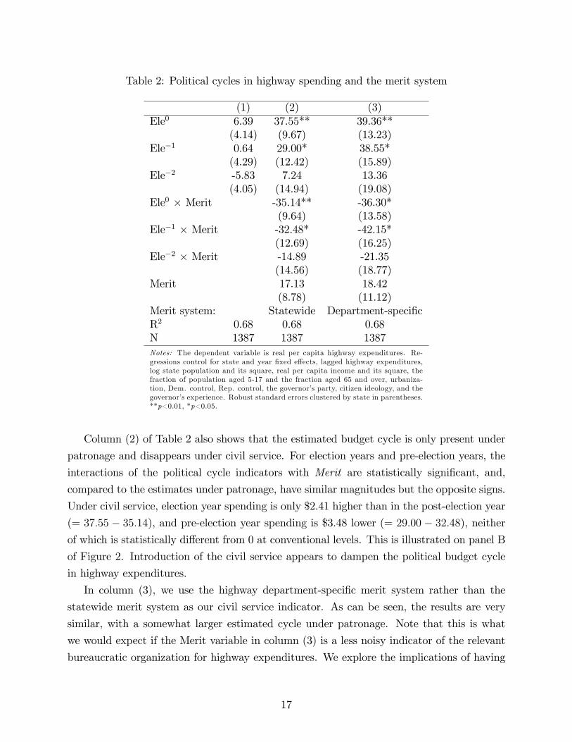
Table 2: Political cycles in highway spending and the merit system

(1) (2) (3)Ele0 6.39 37.55** 39.36**

(4.14) (9.67) (13.23)Ele−1 0.64 29.00* 38.55*

(4.29) (12.42) (15.89)Ele−2 -5.83 7.24 13.36

(4.05) (14.94) (19.08)Ele0 × Merit -35.14** -36.30*

(9.64) (13.58)Ele−1 × Merit -32.48* -42.15*

(12.69) (16.25)Ele−2 × Merit -14.89 -21.35

(14.56) (18.77)Merit 17.13 18.42

(8.78) (11.12)Merit system: Statewide Department-specificR2 0.68 0.68 0.68N 1387 1387 1387Notes: The dependent variable is real per capita highway expenditures. Re-gressions control for state and year fixed effects, lagged highway expenditures,log state population and its square, real per capita income and its square, thefraction of population aged 5-17 and the fraction aged 65 and over, urbaniza-tion, Dem. control, Rep. control, the governor’s party, citizen ideology, and thegovernor’s experience. Robust standard errors clustered by state in parentheses.**p<0.01, *p<0.05.

Column (2) of Table 2 also shows that the estimated budget cycle is only present under

patronage and disappears under civil service. For election years and pre-election years, the

interactions of the political cycle indicators with Merit are statistically significant, and,

compared to the estimates under patronage, have similar magnitudes but the opposite signs.

Under civil service, election year spending is only $2.41 higher than in the post-election year

(= 37.55 − 35.14), and pre-election year spending is $3.48 lower (= 29.00 − 32.48), neither

of which is statistically different from 0 at conventional levels. This is illustrated on panel B

of Figure 2. Introduction of the civil service appears to dampen the political budget cycle

in highway expenditures.

In column (3), we use the highway department-specific merit system rather than the

statewide merit system as our civil service indicator. As can be seen, the results are very

similar, with a somewhat larger estimated cycle under patronage. Note that this is what

we would expect if the Merit variable in column (3) is a less noisy indicator of the relevant

bureaucratic organization for highway expenditures. We explore the implications of having

17

Figure 2: Political cycles in highway spending under civil service and patronage

Notes: The figure shows the political budget cycles in highway expenditures (in real 2009 dollars per

capita) implied by the estimates in Table 2, column (2) under patronage (Panel A) and civil service (Panel

B). In each case the base category is the post-election year, normalized to 0. The 95 percent confidence

interval is shown by the grey lines.

only a department-specific merit system without statewide civil service in section 5.3 below.

Table 3 presents estimates of Eqn. (2). Because the election cycle indicator here is binary

(taking a value of 1 for the pre-election year or the election year), column (1) first shows that

our findings above hold using this indicator as well. Column (2) adds all the interactions

with fixed effects and controls. Here, the reported coeffi cient on the Ele indicator is the

estimated marginal effect when the value of each interacted control and fixed effect is fixed

at its sample mean. We find that the patterns from column (1) are reinforced, with the

coeffi cients on both the election cycle dummy and its interaction with Merit increasing

in size. Columns (3) and (4) repeat these regressions using the department-specific merit

system variable and show similar findings. In all cases we find a significant political budget

cycle under patronage, and this is smoothed out under civil service.

In terms of magnitude, is the political budget cycle uncovered under patronage large

or small? While an extra $30-40 per capita per year would not be much if it was purely

a monetary transfer, here this represents investment in infrastructure that likely has large

positive externalities over many years. Voters’valuation for such an investment is likely

to be much larger than $40. In the absence of applicable welfare measures, a more useful

benchmark may be the 9-12% increase relative to the average post-election year spending.

This is comparable to previous estimates in the literature: Drazen and Eslava (2010) find

a 7% election year effect for urban infrastructure in Colombia, and Khemani (2004) a 9%

effect for capital investment in India.

18

Table 3: Fully interacted specifications

(1) (2) (3) (4)Ele 29.40** 42.70** 32.04** 51.30**

(8.17) (11.90) (11.25) (13.22)Ele × Merit -26.23** -37.19* -28.51* -45.15**

(8.25) (13.83) (11.62) (14.80)Merit 9.81 17.70* 7.86 17.32*

(7.89) (6.88) (8.18) (7.33)Merit system: Statewide Statewide Department-specific Department-specificInteractions with Ele No Yes No YesR2 0.68 0.93 0.68 0.93N 1,387 1,387 1,387 1,387Notes: The dependent variable is real per capita highway expenditures. Ele = 1 in the pre-election or the election yearand 0 otherwise. Columns (2) and (4) include interactions of Ele with all control variables X and state and year fixedeffects. In these regressions reported coeffi cients on Ele are the estimated marginal effects of this indicator when the valueof each interacted variable is fixed at its sample mean. All regressions control for state and year fixed effects, lagged highwayexpenditures, log state population and its square, real per capita income and its square, the fraction of population aged5-17 and the fraction aged 65 and over, urbanization, Dem. control, Rep. control, the governor’s party, citizen ideology,and the governor’s experience. Robust standard errors clustered by state in parentheses. **p<0.01, *p<0.05.

5.2 Robustness

In this section we present several robustness checks on our main result. We focus on the

specification in equation (1) since this is the approach most commonly used in the literature.

We discuss our findinds in the text and provide detailed estimates in the Appendix.

5.2.1 Different samples and estimation method

Because we restrict attention to 4-year gubernatorial terms, the set of states in the sample

changes over time. In particular, some states switch from 2 to 4 year terms during our sample

period, these states therefore only enter the sample in later years. Does the changing set of

states affect our results? We ran regressions on a balanced panel of states, using only the 32

states that had 4-year terms throughout the sample period. Our results are very similar to

those obtained earlier, indicating that the changing set of states does not affect our findings.

Our main estimates covered the period 1960-1995. There are two reasons to wonder

whether the estimates are robust to considering a shorter period. First, the nature of highway

spending changed over time: while the focus in the earlier period was on construction, later

projects were increasingly for maintenance. Dilger (1989) suggests that 1983 was a turning

point in this respect (see also Knight, 2002). Second, the approach to civil service reform

changed over time (see section 2.3). After an emphasis on merit system protections and

bureaucratic independence during the first wave of civil service reforms, the second wave

19

of reforms emphasized accountability to managers and bureaucratic responsiveness. This

led to a weakening of civil service protections. While at the state level the second wave of

reforms did not start until a 1996 reform in Georgia, policy changes at the federal level came

earlier, with the 1978 Civil Service Reform Act. Thus, it may be that the operation of state

bureaucracies in the latter part of the sample (and in particular the 1989 introduction of

the merit system in West Virginia) is less comparable than in earlier years. As a robustness

check, we repeated our regressions shortening the sample period by a third, to 1960-1983.

The findings for this period are very similar to those obtained earlier.

As discussed above, our panel is long enough that any bias in the fixed effects estimates

due to the presence of the lagged independent variable is likely to be minimal. By contrast,

in a panel this long the Arellano-Bond type methods designed to address the bias can be

problematic due to the proliferation of instruments. Nevertheless, to check the robustness

of our findings, we performed various versions of difference GMM estimation. Our findings

reported above appear robust to the use of these different estimation methods.

5.2.2 Controlling for political strength

The political strength of the administration and the competitiveness of elections is a potential

confounder that may affect both the likelihood of civil service reform and the executive’s

ability and incentives for creating budget cycles. For example, if a stronger administration

found it easier to create political budget cycles and civil service reform was more likely under

a weaker administration, then the disappearance of the budget cycle observed above could

be due to a decline in the political strength of the administration, rather than to civil service

reform.23 While the specifications above already include several political controls, we now

present five exercises to further control for this and other potential confounders.

First, we include the winning margin of the incumbent governor from the previous elec-

tion as a further control for the incumbent’s political strength and the competitiveness of

elections. Including this variable either on its own or interacted with the election cycle

indicators does not affect our results. Second, we follow Folke et al. (2011) and drop admin-

istrations elected with relatively wide margins. The idea is that administrations elected with

smaller margins may be more comparable to each other on unobservables (for example, they

may face more similar competitive environments). While the estimates become imprecise as

the sample gets small, restricting attention to winning margins below 20, 10 or 5 percentage

points causes little change in the pattern of our results.24 Third, we exclude states where the

23See Folke et al. (2011) and Ting et al. (2012) for discussions of the relationship between competitivenessand civil service reform.24The pre-election year coeffi cient drops in magnitude for margins below 10 but is large again (though

20

same party held the governor’s seat for a long period of time around civil service reform. In

these cases any changes in political strength may not be adequately captured by our control

variables, we therefore checked whether excluding these states affected our results. In par-

ticular, we excluded states where civil service reform occurred during our sample period and

the same party held the governor’s seat in the 5 years preceding the reform as well as the 5

years following the reform. We find that our findings remain robust. Fourth, also following

Folke et al. (2011), we drop years just before or just after civil service reform. These are the

periods where any confounder correlated with civil service reform may be especially relevant.

Leaving out the period 2, 4, or 6 years before and after reform does not change our findings.

5.3 Further results and mechanisms

5.3.1 Department-specific vs. statewide merit system

How do patterns of highway spending vary under a merit system specific to the highway

department vs. a merit system with statewide coverage? We can explore this question

because we have periods in our data with department-specific merit system but no statewide

civil service (see Table 1). However, since we only have a limited number of these periods (38

state-year observations in four states25), these results should be taken merely as suggestive.

Figure 3 shows the results of estimating equation (1) with both the statewide and the

department-specific merit variables (and their respective interactions with the election cycle).

The parameter estimates are given in the Appendix. In the figure, Panel A is for patronage,

panel B for a department-specific merit system only, and panel C for statewide civil service.

Panels A and C are similar to Figure 2 and show the dampening of the budget cycle under

a statewide merit system compared to patronage. Interestingly, the pattern in Panel B

is somewhere between the two, with no pre-election year increase in spending, but still

a spike in spending in election years. This may suggest that a department-specific merit

system without a statewide merit system dampens the political budget cycle somewhat, but

still leaves opportunities for increased spending, especially closer to the election.26 These

imprecisely estimated) for margins below 5. The coeffi cients on election year and its interaction with meritremain large throughout.25South Carolina, Idaho, Washington, and Texas. Although a fifth state, Arizona, had a department-

specific merit system before statewide civil service was introduced, its governors were serving 2-year termsand is therefore excluded from the sample for that period.26It is possible that politically motivated spending in the pre-election year takes a different form than

election year spending: for example, the former could be weighed towards construction projects, which taketime to yield results, while the latter could be more maintenance work, which can yield electoral benefitsfaster. Figure 3 may suggest that, on its own, a department-specific merit system may constrain the formertype of spending more than the latter. Exploring this further would be an interesting topic for futureresearch.

21

interpretations are subject to the caveat above regarding the small number of observations

in our data that are used to identify the patterns in Panel B.

5.3.2 First-term vs. reelected governors

Governors’ ability to make policy could change with experience. On the one hand, the

governor’s mandate may be stronger after the election than later in the term; on the other

hand, some policies may require time to develop and experience to implement, making them

more likely later in the term. For example, because highway projects take time to develop,

they may be more likely in the second half of a term, i.e., in election years and pre-election

years. To interpret our results above, it is important to know whether political budget cycles

are driven by politicians’incentives to engage in voter-friendly policies, or simply by changes

in their experience. To address this question, in the Appendix we present results controlling

for a more refined measure of governor experience (beyond the linear measure included in

the above regressions). We compare the budget cycle under patronage between first-term

and re-elected governors and find similar results, suggesting that the cycle is unlikely to be

due to changing governor experience and the time it takes to make policy.

5.3.3 The role of the legislature

In line with the political budget cycle literature, we have focused on the electoral cycle of the

chief executive (the governor). As described above, in the context of US highway finance state

legislatures face several constraints in affecting spending decisions. To the extent possible,

we now check whether the limited role of legislatures in this context is also reflected in the

data.

First, we ask whether political budget cycles may be linked to legislative elections. To

do this we must deal with the diffi culty posed by simultaneous elections: election years

for governors are typically also election years for at least some legislators, which makes it

challenging to identify the two electoral effects separately. To make some progress, we use

the fact that in most cases, legislative elections happen biannually, while all governors in our

sample serve 4-year terms. This means that in addition to Ele0, the year Ele−2 is typically

also a legislative election year. As our results in Table 2 show, however, there is an increase

in highway spending in Ele0, the gubernatorial election year, but not in Ele−2, when only

legislative elections are held. In the Appendix, we confirm that this pattern holds if we

exclude from the sample the five states where the house of representatives is elected every

four years. These results provide further support for our focus on the role of the executive

rather than the legislature in creating spending cycles.

22

Figure3:Politicalcyclesinhighwayspendingunderstatewideorhighwaydepartment-specificcivilservice,orpatronage

Notes:Thefigureshowsthepoliticalbudgetcyclesinhighwayexpenditures(inreal2009dollarspercapita)impliedbyestimatesofEquation(1)

thatincludeboththestatewideandthedepartment-specificmeritvariables,andtheirrespectiveinteractionswiththeelectoralcycleindicators.In

eachpanelthebasecategoryisthepost-electionyear,normalizedto0.The95percentconfidenceintervalisshownbythegreylines.

23

While the legislature may not play a direct part in highway spending cycles, it is possible

that it has a mediating role by affecting governors’ability to generate cycles. For example,

cycles may be less likely under divided government when one party controls the legislature

while the other holds the governor’s seat, or under a more professional legislature. We

test for the former possibility by including interactions between the election cycle variables

and an indicator for divided government, and we do not find any significant results. To

study professionalism, we include an index of the professionalism of the legislature from

King (2000), and these estimates are also insignificant. In all these cases our earlier findings

still hold: a civil service system appears to have a bigger role than divided government or

professional legislatures in dampening the political cycle in highway spending.

5.3.4 Toll vs. regular highways

At the most general level, political budget cycles refer to any changes in fiscal categories

correlated with the electoral cycle. Budget cycles can arise from politicians’ and voters’

focus on expenditures or revenues (or both). For example, if cycles reflect politicians’desire

to please voters and voters are “fiscal conservatives”(Peltzman, 1992), politicians’incentive

may be to increase revenues and lower deficits before elections.

Our results above provide evidence of a focus on a particular type of expenditure in the

context of US state politics. However, this interpretation may need to be qualified due to

the presence of toll highways. While toll and non-toll highways are similar in many respects

(including their potential to serve as a vehicle for patronage), there is one crucial difference:

toll highways create revenue for state governments. If the political budget cycle uncovered

above was driven by spending on toll highways, this could indicate that incumbent politicians

are in fact motivated by revenues rather than expenditures.

Because the Census of Governments reports spending on toll and non-toll highways sep-

arately, we can check for this by estimating separate regressions for the two categories. The

results, reported in the Appendix, clearly indicate that the budget cycles under patronage

arise in non-toll highway expenditures. The evidence regarding toll highways is at best in-

conclusive: there are no statistically significant cycles under either patronage or civil service,

but the standard errors are large. Toll highways and an associated desire to increase revenues

does not drive our results above.

24

6 Conclusion

Bureaucratic institutions matter for policy and the behavior of politicians. In this paper we

found that civil service protections can stabilize government activity over time by dampening

the political budget cycle. In particular, we found significant budget cycles in the highway

expenditures of US state governments under patronage but no cycles under civil service.

These findings may suggest a possible explanation for some of the cross-country differ-

ences observed in previous studies: political budget cycles may be more prevalent in political

systems characterized by patronage but less likely to occur under civil service. While the

potential of civil service to stabilize the bureaucracy has long been recognized, our results

suggest that this institution may also have a “multiplier” effect by stabilizing the policies

chosen by election-minded politicians.

References

[1] Akhmedov, A., and E. Zhuravskaya (2004): “Opportunistic Political Cycles: Test in a

Young Democracy Setting,”Quarterly Journal of Economics 119(4), 1301-1338.

[2] Alesina, A., and G. Tabellini (2007): “Bureaucrats or Politicians? Part I: A single

policy task,”American Economic Review 97(1), 169-179.

[3] Alesina, A., and G. Tabellini (2008): “Bureaucrats or politicians? Part II: Multiple

policy tasks,”Journal of Public Economics 92, 426—447.

[4] Alt, J. E., and D.D. Lassen (2006): “Transparency, Political Polarization, and Political

Budget Cycles in OECD Countries,”American Journal of Political Science 50(3), 530-

550.

[5] Alt, J. E., and S. S. Rose (2009): “Context-conditional political budget cycles,” in:

C. Boix and S. C. Stokes (Eds.), The Oxford handbook of comparative politics, Oxford:

Oxford University Press.

[6] Arellano, M., and S. Bond (1991): “Some Tests of Specification for Panel Data: Monte

Carlo Evidence and an Application to Employment Equations,”Review of Economic

Studies 58(2), 277-297.

[7] Berry, W. D., E. J. Ringquist, R. C. Fording, and R. L. Hanson (1998): “Measuring

Citizen and Government Ideology in the American States, 1960-93,”American Journal

of Political Science 42, 327-48.

25

[8] Besley, T., and A. Case (2003): “Political institutions and policy choices: Evidence

from the United States,”Journal of Economic Literature 41, 7-73.

[9] Brender, A., and A. Drazen (2005): “Political Budget Cycles in New versus Established

Democracies,”Journal of Monetary Economics, 52(7), 1271-1295.

[10] Canes-Wrone, B., and J.-K. Park (2012): “Electoral Business Cycles in OECD Coun-

tries,”American Political Science Review 106(1), 103-122.

[11] Congressional Budget Offi ce (1978): Highway Assistance Programs: A Historical Per-

spective, Washington, DC: Congressional Budget Offi ce.

[12] de Haan, J., and J. Klomp (2013): “Conditional political budget cycles: a review of

recent evidence,”Public Choice 157, 387—410.

[13] Dilger, R.J. (1989): National intergovernmental programs, Englewood Cliffs, NJ: Pren-

tice Hall.

[14] Drazen, A. (2001): “The Political Business Cycle after 25 Years,”In B.S. Bernanke and

K.Rogoff (Eds.): NBER Macroeconomics Annual 2000, 75-117, Cambridge, MA: MIT

Press.

[15] Drazen, A., and M. Eslava (2010): “Electoral Manipulation via Voter-Friendly Spend-

ing: Theory and Evidence,”Journal of Development Economics 92(1), 39-52.

[16] Epstein, D., and S. O’Halloran (1999): Delegating Powers. A Transaction Cost Pol-

itics Approach to Policy Making under Separate Powers, Cambridge, UK: Cambridge

University Press.

[17] Eslava, M. (2011): “The Political Economy of Fiscal Deficits: A Survey,” Journal of

Economic Surveys 25(4), 645-673.

[18] Evans, D (1994) “Policy and Pork: The Use of Pork Barrel Projects to Build Coalitions

in the House of Representatives.”American Journal of Political Science 38 (4), 894—917.

[19] Folke, O., S. Hirano, and J. M. Snyder, Jr. (2011): “Patronage and Elections in US

States,”American Political Science Review 105(3), 567-585.

[20] Fox, J., and S.V. Jordan (2011): “Delegation and Accountability,”Journal of Politics

73(3), 831—844.

26

[21] Gailmard, S., and J.W. Patty (2007): “Slackers and Zealots: Civil Service, Policy

Discretion, and Bureaucratic Expertise,”American Journal of Political Science 51(4),

873-889.

[22] Healy, A., and G. Lenz (2014): “Substituting the End for the Whole:Why Voters Re-

spond Primarily to the Election-Year Economy,”American Journal of Political Science

58(1), 31—47.

[23] Holtz-Eakin, D., W. Newey, and H. S. Rosen (1988): “Estimating vector autoregressions

with panel data,”Econometrica 56, 1371—1395.

[24] Ingraham, P.W. (1995): The Foundation of Merit: Public Service in American Democ-

racy, Baltimore, MD: Johns Hopkins University Press.

[25] Judson, R. A., and A. L. Owen (1999): “Estimating Dynamic Panel Data Models: A

Guide for Macroeconomists,”Economics Letters 65(1): 9-15.

[26] Khemani, S. (2004): “Political Cycles in a Developing Economy: Effect of Elections in

the Indian States,”Journal of Development Economics 73(1): 125-154.

[27] King, J.D. (2000): “Changes in Professionalism in U. S. State Legislatures,”Legislative

Studies Quarterly 25(2), 327-343.

[28] Knight, B. (2002): “Endogenous federal grants and crowd-out of state government

spending: theory and evidence from the federal highway aid program,”American Eco-

nomic Review 92(1), 71—92.

[29] Krause, G. A., D. E. Lewis, and J. W. Douglas (2006): “Political appointments, civil

service systems, and bureaucratic competence: Organizational balancing and executive

branch revenue forecasts in the American states,”American Journal of Political Science

50(3), 770-787.

[30] Martin, J.W. (1959): “Administrative Dangers in the Enlarged Highway Program,”

Public Administration Review 19(3), 164-172.

[31] Maskin, E., and J. Tirole (2004): “The Politician and the Judge: Accountability in

Government,”American Economic Review 94(4), 1034-1054.

[32] Mosher, F. (1982): Democracy and the public service, 2nd ed., New York, NY: Oxford

University Press.

27

[33] Nall, C. (2015): “The Political Consequences of Spatial Policies: How Interstate High-

ways Facilitated Geographic Polarization,”Journal of Politics 77(2), 394-406.

[34] National Research Council (1952): Merit System Provisions in State Highway Employ-

ment, Washington, DC: Highway Research Board, NRC.

[35] Ornaghi, A. (2016): “Civil Service Reforms: Evidence from U.S. Police Departments,”

working paper, http://economics.mit.edu/files/12297.

[36] Peltzman, S. (1992): “Voters as Fiscal Conservatives,”Quarterly Journal of Economics

107(2), 327-361.

[37] Persson, T., and G. Tabellini (2003): The Economic Effects of Constitutions, Cam-

bridge, MA: MIT Press.

[38] Rauch, J. E. (1995): “Bureaucracy, infrastructure, and economic growth: Evidence from

US cities during the Progressive era,”American Economic Review 85(4), 968-979.

[39] Rauch, J.E., and P.B. Evans (2000): “Bureaucratic structure and bureaucratic perfor-

mance in less developed countries,”Journal of Public Economics 75, 49-71.

[40] Rogoff, K. (1990): “Equilibrium political budget cycles,”American Economic Review

80, 21—36.

[41] Roodman, D. (2009a): “A Note on the Theme of Too Many Instruments,” Oxford

Bulletin of Economics and Statistics 71(1): 135-158.

[42] Rose, S. (2006): “Do Fiscal Rules Dampen the Political Business Cycle?”Public Choice

128(3-4), 407-431.

[43] Ruhil, A.V.S., and P.J. Camoes (2003): “What Lies Beneath: The Political Roots of

State Merit Systems,” Journal of Public Administration Research and Theory 13(1),

27-42.

[44] Shi, M., and J. Svensson (2006): “Political Budget Cycles: Do They Differ across

Countries and Why?”Journal of Public Economics 90(8-9), 1367-1389.

[45] Sorauf, F.J. (1956): “State Patronage in a Rural County,”American Political Science

Review 50(4), 1046-1056.

[46] Ting, M.M. (2002): “A Theory of Jurisdictional Assignments in Bureaucracies,”Amer-

ican Journal of Political Science 46(2), 364-378.

28

[47] Ting, M.M. (2012): “Legislatures, Bureaucracies, and Distributive Spending,”American

Political Science Review 106(2), 367-385.

[48] Ting, M.M., J.M. Snyder, Jr., S. Hirano, and O. Folke (2012): “Elections and reform:

The adoption of civil service systems in the U.S. states,”Journal of Theoretical Politics

25(3) 363—387.

[49] Tolchin, M., and S. Tolchin (1971): To the Victor... Political Patronage from the Club-

house to the White House, New York, NY: Random House.

[50] Ujhelyi, G. (2014a): “Civil Service Reform,”Journal of Public Economics 118, 15-25.

[51] Ujhelyi, G. (2014b): “Civil Service Rules and Policy Choices: Evidence from US State

Governments,”American Economic Journal: Economic Policy 6(2), 338-380.

29

A Appendix (not for publication)

A.1 Two examples: Texas and Florida

In this section we briefly describe two examples of the political economy of highway admin-

istration, one under a merit system, and one under patronage.

In Texas, the question of whether the Highway Department should be governed by pol-

itics or technical expertise was decided early on in favor of the latter.27 In 1946 (ten years

before the establishment of the federal Highway Trust Fund) a constitutional amendment

was passed establishing a dedicated fund for state highway construction, effectively removing

legislative control over the department’s budget. During the height of highway construction,

the department was led by the same state highway engineer for 27 years (1940-1967).28

The engineer, Dewitt Greer, spent his entire life in highway construction and was promoted

through the ranks. His expertise was widely recognized: at one point President Johnson

offered him the job of Federal Highway Administrator (which he declined), and upon retire-

ment he became Professor of Engineering Practice at the University of Texas.

Both contemporary observers and historians praise Greer’s highway department for its

integrity and professionalism: “In twenty-five years there has not been a breath of scandal

in the department” (Morehead, 1984, 71). Greer “was primarily responsible for selecting

generations of middle-level administrators who have kept the Department out of politics

for more than 30 years.”(Smith, 1974, 13). Running a clean department included keeping

contractors at arm’s length: “A contractor couldn’t buy him a cup of coffee.” (Morehead,

1984, 71).

In this institutional environment, highway construction in Texas was shaped by high-

way department bureaucrats. Instead of highway employees bowing to political demands,

influence often went the other way, with department engineers convincing politicians on the

design of programs and regulations. At one point, Greer convinced the governor’s offi ce

that a farm-to-market roads program being considered should be housed in the Highway

Department instead of being delegated to the counties “so it would be well engineered and

effi ciently constructed”to uniform standards (Morehead, 1984, 56). Greer himself ended up

writing the legislation for this particular program.

The Texas highway program was characterized by a focus on technical considerations and

long-term planning. A chief technical consideration was traffi c safety: the state became a

27The description of the Texas case is based on Smith (1974) and Morehead (1984).28This was in stark contrast to the patronage era of the 1920s, when at one point “in a single biennium

(1925-26) four different men served as Highway Engineer, the Department’s top executive position.”(Smith,1974, 11).

30

pioneer of such regulations as minimum road-width, crash-safe traffi c signs and rail guards,

and road-side plantings to improve visibility and safety. Long-term planning is exemplified

by the fact that more than a decade before the start of the interstate highway program

Texas was preparing for the post-war period and “led the nation in planning for a massive

expansion of the highway system after the war.”(Morehead, 1984, 49).

During the same period, highway administration in Florida followed a very different

path.29 Before the introduction of statewide civil service in 1967, highway projects were

political tools administered directly from the governor’s offi ce. With no civil service system,

offi cials who did not comply with politicians’ requests could be fired or suspended. One

senior offi cial recalled being reprimanded by the governor for his lack of cooperation “when

he sent a contractor to see me to get some special consideration”and “when he asked to have

a property assessment raised for a friend of his on the [path of the proposed] Jacksonville

Expressway.”30 Contractors working on highway projects were expected to pay campaign

contributions to relevant politicians, and made “payments of cash, whisky, turkey, and other

merchandise of substantial value to offi cials and employees of the State road department.”31

In this system, the location and implementation of highway projects often reflected var-

ious political goals, from catering to voter interests through pleasing powerful political sup-

porters. Under one administration, road construction primarily targeted two counties: one

was the governor’s home county, the other the home county of his appointed road board

chairman. In the latter case, state highway funds were also used to purchase right-of-way

through the chairman’s own property (Whitney, 2008, p19-20).

As political goals shifted, so did the projects. In 1954, a senator summarized the situation

as follows “A governor appoints a road board that develops a program that fits in with his

ideas. That program is just under way well when a new governor is elected. He names

his own road board, [...] throws out the old program and starts one of its own.” (quoted

in Whitney, 2008, 26). Observers noted an overall lack of long-term planning with new

projects rushed through right-of-way acquisitions and engineering planning in as little as a

few days (Whitney, 2008, 73). A striking contrast with Texas’s anticipation of the federal

highway program is Florida’s focus on state-administered toll highways. Even as the federal

interstate system was being developed in the 1950s, Florida invested heavily in extending its

own turnpikes with the governor unwilling to give up on the state system. At one point, a

long section of the turnpike and the interstate were planned to run in close proximity, parallel

to each other. Eventually the two systems were integrated, but some observers estimated

29The description of the Florida case is based on Whitney (2008) and the references therein.30“Simpson Cites the Record,”Tampa Morning Tribune, April 20 1954, p8.31US Congressional Record - House of Representatives, Vol 109, part 1, January 24, 1963, p952.

31

that Florida lost tens of millions in federal highway aid in the process (Whitney, 2008, 61).32

A.2 Robustness of the main result

Tables 4-7 contain the results referred to in section 5.2 of the paper. In Table 4, column

(1) shows results for the balanced panel that uses only the 32 states which had 4-year

gubernatorial terms throughout the period of study. The following states switched from 2 to

4 year cycles during our study period (with the year of the switch given in parentheses): AZ

(1970), AR (1986), IA (1974), KS (1974), MA (1966), MI (1966), MN (1962), NM (1970),

ND (1964), SD (1974), TX (1974), WI (1970). Column (1) excludes these 12 states from the

analysis.33 Using all states, column (2) shows results for the shorter, 1960-1983 time period.

Table 5 shows our estimates of different GMM specifications. For this approach, one first

differences equation (1) to eliminate the state fixed effects:

∆yst =0∑

τ=−2∆(ατEle

τst + βτEle

τst ×Meritst) + γ∆Meritst

+δ∆ys,t−1 + ∆X ′stρ+ ∆µt + ∆εst.

Then, observing that ∆ys,t−1 and ∆εst are necessarily correlated, higher lags of yst are used

as instruments for ∆ys,t−1.

Column (1) of Table 5 follows the Anderson and Hsiao (1982) approach and uses lags

t − 2 and t − 3 as “standard” instruments. The coeffi cient estimates on the variables of

interest are similar to those obtained above, but the overidentification test fails, indicating

that some of the instruments may not be exogenous. A test of serial correlation indicates

that the presence of 2nd order autocorrelation has a p-value of 0.10, suggesting that using

the t− 2 lag as an instrument may not be appropriate. The next column uses lags t− 3 and

t− 4 as instruments, resulting in better model performance (and broadly similar coeffi cient

estimates). In column (3) we use the same lags but treat each year as a separate equation

following the Arellano and Bond (1991) method. As can be seen, our results are very similar.

32The reason behind Florida’s focus on state turnpikes is likely a combination of factors. A benevolentinterpretation is that this afforded the governor an opportunity to bypass much of the state’s corrupt highwayadministration and work with a team of professional experts instead (including consultants from other statesand experienced investors). Another possibility is that governors wanted to cater to their own special interestgroups that favored the turnpike, or that they wanted to avoid the federal scrutiny that would come withusing federal funds.33Two states, Florida and Illinois, had 4-year terms throughout the sample period but moved gubernatorial

elections from presidential election years to midterm election years (in 1966 and 1978, respectively). In bothcases this resulted in one 2-year term for the governor in offi ce at the time of the change and throughout theanalysis we exclude these 2-year terms from the sample for these states (but include all other terms).

32

Table 4: Balanced panel and shorter time period

Balanced panel Before 1983(1) (2)

Ele0 38.39** 44.75**(12.79) (12.39)

Ele−1 26.70* 32.01*(11.81) (12.86)

Ele−2 15.51 7.52(17.70) (13.98)

Ele0 × Merit -38.40** -34.35**(12.60) (11.66)

Ele−1 × Merit -32.18* -34.46*(11.95) (13.46)

Ele−2 × Merit -24.58 -14.30(17.35) (14.69)

Merit 20.46* 15.00(9.72) (10.08)

R2 0.72 0.68N 1,110 862Notes: The dependent variable is real per capita highway expenditures. Column (1)restricts attention to states with 4-year gubernatorial terms throughout the sampleperiod. Column (2) restricts attention to 1960-1983. All regressions control for stateand year fixed effects, lagged highway expenditures, log state population and itssquare, real per capita income and its square, the fraction of population aged 5-17and the fraction aged 65 and over, urbanization, Dem. control, Rep. control, thegovernor’s party, citizen ideology, and the governor’s experience. Robust standarderrors clustered by state in parentheses. **p<0.01, *p<0.05.

Finally, in column (4) we include further lags (up to t−10) and again find that the coeffi cients

of interest change very little.

33

Table5:Politicalcyclesinhighwayspendingandthemeritsystem,GMMestimates

Estimationmethod

Anderson-Hsiao

Anderson-Hsiao

Arellano-Bond

Arellano-Bond

(1)

(2)

(3)

(3)

Ele0

41.21*

36.78**

36.00**

39.30**

(17.65)

(13.31)

(12.28)

(11.28)

Ele−1

33.34

23.98

27.70*

29.80*

(21.91)

(13.49)

(13.17)

(13.16)

Ele−2

8.95

5.98

6.75

8.54

(16.86)

(11.06)

(13.49)

(14.43)

Ele0×Merit

-33.49*

-31.52*

-31.65**

-34.82**

(16.26)

(12.91)

(11.58)

(10.14)

Ele−1×Merit

-34.65*

-25.84*

-30.64**

-32.25**

(20.33)

(13.21)

(13.07)

(12.79)

Ele−2×Merit

-15.04

-11.12

-13.70

-15.27

(17.13)

(11.49)

(12.96)

(13.74)

Merit

28.12

26.86

22.43

11.10

(31.06)

(25.37)

(22.47)

(18.62)

Lagsusedasinstruments

2,3

3,4

3,4

3-10

Overidentificationtestp-value

0.08

0.44

aa

Testof1storderserialcorrelation

0.21

0.03

0.00

0.00

Testof2ndorderserialcorrelation

0.10

0.06

0.05

0.06

Testof3rdorderserialcorrelation

0.77

0.89

0.95

0.86

Testof4thorderserialcorrelation

0.74

0.74

0.73

Numberofinstruments

5252

115

280

N1307

1275

1339

1339

Notes:Thedependentvariableisrealpercapitahighway

expenditures.

GMMestimateson

firstdifferencesusinglagsofthedependent

variableasAnderson-HsiaoorArellano-Bondstyleinstruments.Reportedmodeldiagnosticsarethep-valuesfrom

Hansen’sJ-statisticand

from

Arellano-Bond’sautocorrelationtests.Columns(3-4)andtheautocorrelationtestsusextabond2inStata(Roodman,2009b).Regressions

controlforstateandyearfixedeffects,laggedhighwayexpenditures,logstatepopulationanditssquare,realpercapitaincomeanditssquare,

thefraction

ofpopulation

aged

5-17

andthefraction

aged

65andover,urbanization,Dem.control,Rep.control,thegovernor’sparty,

urbanization,citizenideology,andthegovernor’sexperience.Robuststandarderrorsinparentheses.**p<0.01,*p<0.05.

aWithalargenumberofinstrumentsHansen’sJ-statisticistooweaktobemeaningful(p=1.00).

34

Table 6 controls for the winning margin of the current governor in the last election (dif-

ference between the vote shares of the winner and runner-up). Column (1) includes winning

margin as a simple control, column (2) interacts it with the election cycle indicators,34 column

(3) restricts the sample to winning margins of no more than 20 percentage points, column

(4) restricts to no more than 10, and column (5) to no more than 5 percentage points.

Table 6: Controlling for winning margins

(1) (2) (3) (4) (5)Ele0 37.73** 37.60** 44.92** 51.91** 51.57

(9.93) (10.81) (10.73) (14.91) (32.80)Ele−1 28.44* 28.78* 30.21* 16.38 41.24

(12.65) (12.85) (13.26) (15.92) (32.22)Ele−2 6.92 6.85 14.43 10.15 26.77

(15.26) (15.66) (15.77) (17.88) (27.14)Ele0 × Merit -34.98** -35.48** -44.34** -50.54** -48.26

(9.81) (10.63) (10.99) (15.34) (32.78)Ele−1 × Merit -31.82* -32.18* -34.18* -23.71 -53.69

(12.92) (13.12) (14.44) (17.51) (35.57)Ele−2 × Merit -14.46 -14.98 -24.33 -22.65 -36.68

(14.84) (15.18) (15.57) (18.25) (28.88)Merit 16.50 17.03 12.68 21.66 -4.04

(8.88) (8.96) (10.94) (19.00) (32.98)R2 0.93 0.93 0.69 0.75 0.67N 1,387 1,387 1,008 611 301Winning margin cutoff None None 20 ppoints 10 ppoints 5 ppointsNotes: The dependent variable is real per capita highway expenditures. Column (1) controls for the governor’swinning margin in the last election, and column (2) also includes interactions of winning margin with the electoralcycle indicators. Columns (3)-(5) drop elections with wide margins from the sample (above 20, 10, and 5 percentagepoints, respectively). All regressions control for state and year fixed effects, lagged highway expenditures, log statepopulation and its square, real per capita income and its square, the fraction of population aged 5-17 and thefraction aged 65 and over, urbanization, Dem. control, Rep. control, the governor’s party, citizen ideology, and thegovernor’s experience. Robust standard errors clustered by state in parentheses. **p<0.01, *p<0.05.

In Table 7, column (1) excludes states where civil service reform occurred during our

sample period and the same party held the governor’s seat in the 5 years preceding the

reform as well as the 5 years following the reform (Kentucky, Mississippi, Montana, North

Dakota, and South Carolina). Columns (2-4) exclude years just before and just after civil

service reform.

34Here, reported coeffi cients on the election cycle indicators are the estimated marginal effects of theseindicators when winning margin is fixed at its sample mean.

35

Table 7: Further robustness checks

Changes in Without years around reformgovernor’s party

(1) (2) (3) (4)Ele0 50.17** 42.06** 34.18** 33.55*

(12.16) (11.88) (10.97) (13.65)Ele−1 32.18* 38.57* 29.59 28.40

(13.20) (17.99) (15.02) (15.26)Ele−2 22.08 16.84 15.90 7.06

(19.54) (12.84) (12.33) (16.21)Ele0 × Merit -48.31** -37.89** -30.66** -29.55*

(11.33) (11.62) (10.42) (12.97)Ele−1 × Merit -33.00* -40.58* -31.41 -30.32

(13.77) (18.30) (15.62) (15.18)Ele−2 × Merit -25.57 -22.10 -21.89* -11.44

(19.06) (13.31) (12.85) (16.37)Merit 20.18 15.23 11.79 20.60

(11.03) (13.61) (15.57) (20.84)R2 0.69 0.69 0.68 0.68N 1,219 1,332 1,285 1,237Years before/after 2 4 6reform droppedNotes: The dependent variable is real per capita highway expenditures. Column (1) exludes stateswhere the governor’s party affi liation is unchanged in the decade around reform, and columns (2)-(4)drop years within the specified window around civil service reform (plus or minus 2, 4, or 6 years,respectively). All regressions control for state and year fixed effects, lagged highway expenditures,log state population and its square, real per capita income and its square, the fraction of populationaged 5-17 and the fraction aged 65 and over, urbanization, Dem. control, Rep. control, the governor’sparty, citizen ideology, and the governor’s experience. Robust standard errors clustered by state inparentheses. **p<0.01, *p<0.05.

36

A.3 Further results

Tables 8-12 contain the results described in section 5.3. Table 8 contains the regression

estimates used to construct Figure 3.

Table 8: Political cycles under statewide or department-specific merit systems

Ele0 39.30**(13.19)

Ele−1 38.54*(15.84)

Ele−2 13.94(19.14)

Ele0 × Merit -32.14**(7.45)

Ele−1 × Merit -13.17(11.37)

Ele−2 × Merit 1.25(7.28)

Merit 17.49(9.65)

Ele0 × HwyMerit -4.84(15.49)

Ele−1 × HwyMerit -29.31(19.62)

Ele−2 × HwyMerit -23.27(19.92)

HwyMerit 1.80(14.02)

R2 0.69N 1387Notes: The dependent variable is real per capita highway expenditures.HwyMerit = 1 if a department-specific merit system is in place. The regres-sion controls for state and year fixed effects, lagged highway expenditures, logstate population and its square, real per capita income and its square, thefraction of population aged 5-17 and the fraction aged 65 and over, urban-ization, Dem. control, Rep. control, the governor’s party, citizen ideology,and the governor’s experience. Robust standard errors clustered by state inparentheses. **p<0.01, *p<0.05.

Table 9 focuses on governor experience. We use the fact that governors who already served

a previous term are more experienced than first-term governors, and create an indicator for

governors who are serving their 2nd or more term (whether consecutive or not). In our data,

every state except Mississippi has had governors serving 2 or more terms, with a total of 158

37

elections won by governors who already served.35 If the budget cycle in highway spending

uncovered above was driven by experience, we would expect it to be less pronounced under

governors serving their second or more term. Table 9 asks whether this is the case by

interacting this indicator with the election cycle variables in our main regressions. The first

set of coeffi cients presented is for the electoral cycle under first-term governors, while the

second set is for re-elected governors. In columns (2) and (3), the third set of coeffi cients

are the interactions with the civil service measures (statewide in column 2 and department-

specific in column 3). Column (1) shows no clear budget cycle on average under either

first-term or re-elected governors. Columns (2) and (3) indicate that, once bureaucratic

organization is controlled for, the budget cycle in patronage states is present both under

first-term governors and re-elected governors. Furthermore, the magnitude of the cycle shows

little difference between the two types of governors (none of the differences are statistically

significant at conventional levels). This suggests that the cycle is unlikely to be due to

changing governor experience and the time it takes to make policy.

We also tried running our regressions restricting the sample to re-elected governors (Table

10) but in this smaller sample the standard errors were too large to yield conclusive results.

Table 11 investigates the role of state legislatures. Column (1) restricts attention to

states where the lower house is elected for 2-year terms (in years Ele0 and Ele−2). Excluded

states are Alabama, Louisiana, Maryland, Mississippi, and North Dakota where represen-

tatives serve 4-year terms. The results confirm that highway spending follows the 4-year

gubernatorial cycle, not the 2-year legislative cycle.

Column (2) includes an indicator for divided government and its interaction with the

electoral cycle variables. This indicator is 1 when one party has a majority in both houses of

the state legislature and the other party controls the governor’s seat. The new coeffi cients are

small and not statistically significant, while our earlier findings on civil services vs patronage

remain robust in this specification.

Column (3) includes an index that measures the professionalism of the state legislature.

The index was created by King (2000) based on Squire (1992) and captures the degree of

professionalism based on legislators’compensation, the legislature’s days in session, and its

expenditures for services and operations per legislator. It is available for 4 periods: 1963-64,

1973-74, 1983-84, and 1993-94, and we use linear interpolation to fill in the missing values.36

As above, the new coeffi cients are not significant while our earlier findings remain robust.

Table 12 contains the results for toll and non-toll highways.

35This includes non-elected previous terms, e.g., if a sitting governor dies, is replaced by the lieutenantgovernor, who is then elected in his own right.36In our sample, the range of the index is [0.048, 0.9], with a mean of 0.241 and a std. deviation of 0.138.

38

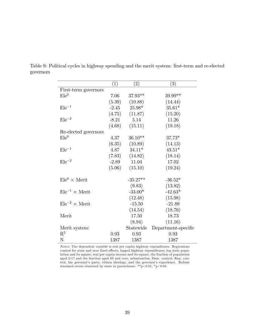
Table 9: Political cycles in highway spending and the merit system: first-term and re-electedgovernors

(1) (2) (3)First-term governorsEle0 7.06 37.93** 39.99**

(5.39) (10.88) (14.44)Ele−1 -2.45 25.98* 35.61*

(4.75) (11.87) (15.20)Ele−2 -8.21 5.14 11.26

(4.68) (15.11) (19.18)Re-elected governorsEle0 4.37 36.10** 37.73*

(6.35) (10.89) (14.13)Ele−1 4.87 34.11* 43.51*

(7.83) (14.82) (18.14)Ele−2 -2.89 11.04 17.02

(5.06) (15.10) (19.24)

Ele0 × Merit -35.27** -36.52*(9.83) (13.82)

Ele−1 × Merit -33.00* -42.63*(12.48) (15.98)

Ele−2 × Merit -15.50 -21.89(14.54) (18.76)

Merit 17.50 18.73(8.94) (11.16)

Merit system: Statewide Department-specificR2 0.93 0.93 0.93N 1387 1387 1387Notes: The dependent variable is real per capita highway expenditures. Regressionscontrol for state and year fixed effects, lagged highway expenditures, log state popu-lation and its square, real per capita income and its square, the fraction of populationaged 5-17 and the fraction aged 65 and over, urbanization, Dem. control, Rep. con-trol, the governor’s party, citizen ideology, and the governor’s experience. Robuststandard errors clustered by state in parentheses. **p<0.01, *p<0.05.

39

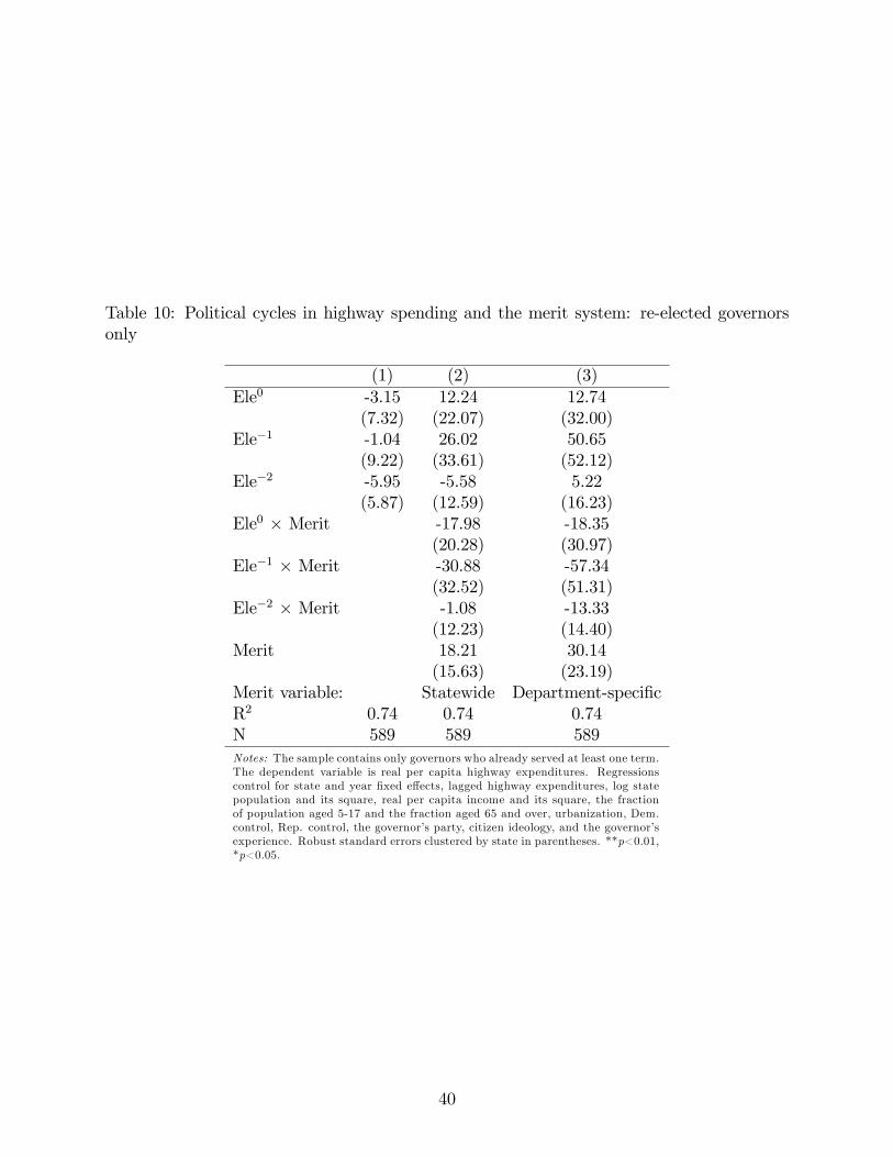
Table 10: Political cycles in highway spending and the merit system: re-elected governorsonly

(1) (2) (3)Ele0 -3.15 12.24 12.74

(7.32) (22.07) (32.00)Ele−1 -1.04 26.02 50.65

(9.22) (33.61) (52.12)Ele−2 -5.95 -5.58 5.22

(5.87) (12.59) (16.23)Ele0 × Merit -17.98 -18.35

(20.28) (30.97)Ele−1 × Merit -30.88 -57.34

(32.52) (51.31)Ele−2 × Merit -1.08 -13.33

(12.23) (14.40)Merit 18.21 30.14

(15.63) (23.19)Merit variable: Statewide Department-specificR2 0.74 0.74 0.74N 589 589 589Notes: The sample contains only governors who already served at least one term.The dependent variable is real per capita highway expenditures. Regressionscontrol for state and year fixed effects, lagged highway expenditures, log statepopulation and its square, real per capita income and its square, the fractionof population aged 5-17 and the fraction aged 65 and over, urbanization, Dem.control, Rep. control, the governor’s party, citizen ideology, and the governor’sexperience. Robust standard errors clustered by state in parentheses. **p<0.01,*p<0.05.

40

Table 11: The role of state legislatures

2-year house Divided Legislatureelections only government professionalism

(1) (2) (3)Ele0 43.65** 37.82** 34.69**

(10.19) (9.52) (9.85)Ele−1 26.17* 28.22* 24.95

(11.28) (12.62) (13.17)Ele−2 15.60 5.75 7.35

(16.87) (14.68) (15.19)Ele0 × Merit -43.74** -35.14** -36.29**

(9.71) (9.61) (10.07)Ele−1 × Merit -30.51* -32.55* -34.28*

(11.37) (12.61) (13.19)Ele−2 × Merit -22.91 -14.97 -15.02

(16.12) (14.45) (14.80)Merit 18.76 17.27 17.96

(10.14) (8.77) (8.96)Ele0 × Divided -0.82

(7.48)Ele−1 × Divided 2.97

(6.77)Ele−2 × Divided 5.53

(7.59)Divided 0.64

(5.44)Ele0 × Prof 17.46

(17.68)Ele−1 × Prof 25.68

(25.10)Ele−2 × Prof 0.06

(22.45)Prof -10.43

(66.06)R2 0.70 0.69 0.69N 1,216 1,387 1,387Notes: The dependent variable is real per capita highway expenditures. Column (1) restrictsattention to states with 2-year terms for house representatives. Divided is 1 if the legislatureand the governor’s seat are controlled by different parties. Prof is an index of the legislature’sprofessionalism. All regressions control for state and year fixed effects, lagged highway expen-ditures, log state population and its square, real per capita income and its square, the fractionof population aged 5-17 and the fraction aged 65 and over, urbanization, Dem. control, Rep.control, the governor’s party, citizen ideology, and the governor’s experience. Robust standarderrors clustered by state in parentheses. **p<0.01, *p<0.05.

41

Table 12: Political cycles in toll vs. non-toll highway spending and the merit system

Dep. Var.: Toll highways Non-toll highways(1) (2)

Ele0 6.61 30.76**(7.60) (7.67)

Ele−1 6.15 22.34(5.28) (11.22)

Ele−2 2.52 4.18(2.23) (14.18)

Ele0 × Merit -4.70 -30.36**(7.69) (8.08)

Ele−1 × Merit -5.65 -26.41*(5.16) (12.02)

Ele−2 × Merit -2.08 -12.39(2.13) (13.96)

Merit 3.85 13.02*(2.70) (7.44)

R2 0.39 0.68N 1387 1387Notes: The dependent variable is real per capita highway expenditures on tolland non-toll highways, respectively. Regressions control for state and yearfixed effects, the lagged value of the dependent variable, log state populationand its square, real per capita income and its square, the fraction of populationaged 5-17 and the fraction aged 65 and over, urbanization, Dem. control, Rep.control, the governor’s party, citizen ideology, and the governor’s experience.Robust standard errors clustered by state in parentheses. **p<0.01, *p<0.05.

42

A.4 Non-highway spending

Are there political budget cycles (conditional on bureaucratic organization) in other spending

categories? While this is a natural question, there are many possible spending categories. To

avoid spurious results due to multiple testing, it is important that the spending categories

tested be chosen based on a priori considerations.

In the case of highway spending, the Interstate Highway Program made road construction

politically salient to voters, and the technical nature of highway projects means that project

implementation can be expected to differ substantially when guided by independent bureau-

crats vs. politicians. Based on these features, there is a priori ground to believe both that

political budget cycles in highway spending are likely, and that these could be conditional on

bureaucratic organization. Furthermore, our data collection on highway department merit

systems ensures that we can study the bureaucratic organization that is most relevant for

highway expenditures. Without further research, it is unclear whether a priori one should

expect to find similar or different results for other spending categories.

With these caveats, we now ask two questions: Are the political budget cycles in highway

expenditures under patronage large enough to show up in total government spending? Do

cycles appear in other spending categories as well? Table 13 provides some answers to these

questions. Column (1) indicates the presence of cycles in total expenditures under patronage

(but not under civil service). Column (2) further shows that this is entirely driven by highway

spending: restricting attention to non-highway expenditures shows no cycles. In Table 14 we

present similar regressions for each major non-highway spending category separately. The

only category for which we find patterns similar to highway expenditures is spending on

hospitals, but the cycle is much smaller (around $4 per capita, or a 3% increase compared

to the post-election year).

Why does the data not show a clear political budget cycle for other expenditure cate-

gories? As discussed above, this question requires further research on each specific category.

Speculatively, some possible answers include the following.

First, it could be that there are political budget cycles in some categories, but the amount

of spending is simply too small to detect them. Second, it could be that the above a priori

considerations, political importance and bureaucratic discretion, simply do not hold for

these other categories in this context. In signaling models a la Rogoff (1990), cycles are

driven by voter expectations: if voters expect a more desirable type of politician to spend

on a certain budget category, then the political budget cycle will manifest itself in that

category. It could be that, during our period of study, the attention given to the Interstate

Highway program made highways a focal point for voters and politicians, and made the

other spending categories in Table 14 relatively less important politically. Of course, once a

43

particular spending category becomes focal, it is not surprising that we do not see a cycle

in all spending categories: if governors spend on roads in election years, they cannot spend

that money on other categories.

Even if a spending category is politically important, we should not expect to find the same

results as for highways unless bureaucrats at the state level play a major role in that category.

For example, education is highly decentralized, and the organization of school districts may

matter more for education spending than the organization of the state bureaucracy. School

districts typically run their own merit system, thus we should not expect the statewide

merit systems studied here to have a major impact in this category. Similarly, some state-

level departments may have already introduced a civil service system before the statewide

reform, and our findings above suggest that this could matter (Figure 3). For example, if fire

departments and the state police are already under civil service, then spending on Public

Safety may be less responsive to the statewide civil service reforms studied here. While

we know - from the information collected here - that most highway departments did not

have their own merit system before the statewide civil service was introduced, there is little

information available in the literature on other departments. Future work to collect this

type of information on departments other than Highways would be useful in understanding

whether one should or should not expect budget cycles in other spending categories.

44

Table 13: Total expenditures and non-highway expenditures

Dep. Var.: Total expenditures Non-highway expenditures(1) (2)

Ele0 30.13 -9.20(15.91) (12.76)

Ele−1 45.95* 12.97(19.83) (12.53)

Ele−2 4.75 -4.52(21.33) (14.60)

Ele0 × Merit -21.79 13.25(16.66) (14.26)

Ele−1 × Merit -58.89* -23.78(24.95) (16.80)

Ele−2 × Merit -25.74 -9.23(23.42) (14.62)

Merit 75.61** 49.69*(27.87) (21.20)

R2 0.98 0.98N 1,387 1,387Notes: The dependent variable is real per capita total direct expenditures in column (1) andreal per capita non-highway direct expenditures in column (2). Regressions control for stateand year fixed effects, the lagged value of the dependent variable, log state population andits square, real per capita income and its square, the fraction of population aged 5-17 and thefraction aged 65 and over, urbanization, Dem. control, Rep. control, the governor’s party,citizen ideology, and the governor’s experience. Robust standard errors clustered by state inparentheses. **p<0.01, *p<0.05.

45

Table14:Politicalcyclesinotherexpenditurecategories

Dep.Var.:

Education

Welfare

Hospitals

Publicsafety

Administration

Nat.resources

(1)

(2)

(3)

(4)

(5)

(6)

Ele0

-5.97

-0.36

4.37*

2.50

0.42

-2.30*

(4.46)

(6.36)

(2.35)

(1.99)

(0.94)

(1.12)

Ele−1

9.48

-0.65

3.75*

0.43

2.72*

-1.37

(5.05)

(3.24)

(1.74)

(0.62)

(1.05)

(1.38)

Ele−2

-9.64

1.48

3.25

-0.01

-0.52

-0.15

(12.18)

(6.40)

(2.51)

(1.35)

(1.28)

(1.91)

Ele0×Merit

11.42*

3.09

-4.61

-1.43

-0.10

2.36

(4.46)

(6.15)

(2.29)

(1.90)

(1.09)

(1.34)

Ele−1×Merit

-6.56

-5.74

-4.57*

-0.13

-2.02

2.65

(5.59)

(5.72)

(2.02)

(0.93)

(1.30)

(2.07)

Ele−2×Merit

9.88

-4.25

-3.47

0.07

-0.37

-0.02

(11.97)

(6.54)

(2.69)

(1.37)

(1.29)

(1.57)

Merit

9.48

12.29

1.37

0.29

2.04

4.64

(7.49)

(10.58)

(2.47)

(1.99)

(1.55)

(3.00)

R2

0.93

0.97

0.90

0.95

0.95

0.70

N1387

1387

1387

1355

1387

910

Post-electionmean

454.86

409.34

121.62

85.28

80.39

66.49

Notes:Thedependentvariableisrealpercapitaexpenditureintheindicatedcategory.Regressionscontrolforstateandyearfixedeffects,the

laggedvalueofthedependentvariable,logstatepopulation

anditssquare,realpercapitaincomeanditssquare,thefraction

ofpopulation

aged5-17andthefractionaged65andover,urbanization,Dem.control,Rep.control,thegovernor’sparty,citizenideology,andthegovernor’s

experience.Post-election

meanshowstheaveragevalueofthedependentvariableinthepost-election

yearsinthesample.Robuststandard

errorsclusteredbystateinparentheses.**p<0.01,*p<0.05.

46

A.5 Data sources, definitions, and summary statistics

Statewide merit systemsSee Ujhelyi (2014b) and the sources reported there.

Highway department merit systemsArizona. “Arizona Highway Changes Proposed,”Prescott Evening Courier, Jan 19, 1955,

p4. “State Highway Examination Dates Are Set,”Prescott Evening Courier, Jul 9, 1957, p8.

Arkansas. “Suggestion To Revamp Road System Heard,”Northwest Arkansas Times, Feb

16, 1952, p1. “Legislature,”The Courier News, Feb 28, 1957, p8.

Delaware. “Stalling on Merit System, du Pont Says of Democrats,”The News Journal, Oct

11, 1961, p10.

Florida. Whitney, J.C. (2008): Florida expressways and the public works career of Congress-

man William C. Cramer, MA thesis, University of South Florida.

Idaho. Fifty Years of Professional Engineering in Idaho, 1960, Boise, ID: Idaho Society of

Professional Engineers. 100th Anniversary, 2010, Boise, ID: Idaho Society of Professional

Engineers.

Iowa. “Murray: Want Possible Hoffa-Roads Tieup?”Ames Daily Tribune, Oct 21, 1958, p1.

“Ending Road Works Spoils,”The Des Moines Register, Sep 22, 1967, p4.

Kentucky. “Combs Plans Merit System,”Kentucky New Era, Apr 10, 1959, p17.

Mississippi. “Highway Problems Aired,” The Delta Democrat-Times, Jul 13, 1973, p16.

“Expanded Merit System Passed,”Clarion-Ledger, Feb 11, 1977, 12C.

Montana. “Commission Will Speed Up State Highway Program,”The Independent Record,

Dec 18, 1962, p1.

New Mexico. “State Highway Department Has A Record Turnover,”Albuquerque Journal,

Nov 18, 1951, p6.

Oklahoma. Odell, W.H. (1950): The patronage system in Oklahoma. Norman, OK: Tran-

script Co.

Pennsylvania. Martin, J.W. (1959): “Administrative Dangers in the Enlarged Highway

Program,”Public Administration Review 19(3), 164-172.

Texas. Smith, G. Jr. (1974): “The Highway Establishment and How it Grew and Grew and

Grew,”Texas Monthly 2(4), April, p76-93. http://www.texasmonthly.com/issue/april-1974.

Morehead, R. (1984): Dewitt C. Greer, King of the Highway Builders, Austin, TX: Eakin

Press.

Utah. “Merit System Triggers Organizational Dispute,”The Deseret News, Dec 24, 1962,

pB-1.

47

South Carolina. “Thurmond Hails Road Department Merit System,”The Index-Journal,

Sep 23, 1950, p5. NRC (1952).

Washington. A History of Personnel Systems for Washington State, 1989, Olympia, WA:

Washington State Department of Personnel.

West Virginia. “Wright Asks All Highway Workers in U.S. Put Under Merit System,”The

Raleigh Register, Jul 25, 1962, p2. “Jay Names Civil Service Commission,”The Raleigh

Register, Jun 28, 1977, p6.

Consumer Price IndexU.S. Department of Labor: Bureau of Labor Statistics, http://www.bls.gov. Consumer Price

Index for All Urban Consumers, not seasonally adjusted. Annual value obtained by averaging

across months. 2009 = 100.

State expendituresUS Census Bureau, State Government Finances Publication Historical Data Base, state

government variables. Direct Expenditure, Regular Hwy-Direct Exp, Total Hwy-Direct Exp,

Total Hwy-Total Exp, Toll Hwy-Total Exp.

Income and populationBureau of Economic Analysis: Regional Economic Accounts, http://www.bea.gov/regional/spi/.

State Annual personal income. Population figures reported in this source are midyear esti-

mates of the Census Bureau.

Aged and kidsUS Census Bureau. The post-1970 data was compiled by List, J.A., and D.M. Sturm (2006).

The pre-1970 was entered from Population Projection (P25) Reports. Year 1969 linearly

interpolated.

Percent urbanUS Census Bureau. Urban and Rural Population 1900-1990, released 1995, available at

http://www.census.gov/population/censusdata/urpop0090.txt. Years between censuses were

linearly interpolated.

Party control and governor’s partyBurnham, W. Dean, “Partisan Division of American State Governments, 1834-1985,”Con-

ducted by Massachusetts Institute of Technology, ICPSR ed. Ann Arbor, MI: Interuniversity

Consortium for Political and Social Research [producer and distributor], 1986. All variables

merged so that they reflect party composition for the given year (for election years, party

48

composition reflects the pre-election situation). Before 1975, this requires shifting the vari-

ables forward by 1 year. Governor’s party: corrections as listed in Ujhelyi (2014b).

Years 1985-1996 from Council of State Governments: Book of the States, various volumes.

Citizen ideologyBerry et al. (1998). This index uses ideological ratings of congressional candidates by the

Americans for Democratic Action and the AFL/CIO’s Committee on Political Education

and their vote shares to estimate the ideological composition of electoral districts; these are

then aggregated to form a statewide measure of citizens’ideology (degree of liberalism, on

a scale 0-100).

Governor’s experienceSource: https://en.wikipedia.org/wiki/List_of_Governors_of_[state] pages. We count the

number of years since a governor first took offi ce (consecutive terms only). When a governor

resigns or dies and is replaced by a member of the administration (usually the lieutenant

governor), we continue the count as if the same person was still in offi ce. To create the

“re-elected”measure used for the additional results in section 5.3.2, we count terms instead

of years, and we also count non-consecutive terms.

49

Table15:Variabledefinitionsandsummarystatistics

Variable

Definition

Mean

Std.Dev.

Min

Max

Highwayexpenditures

Realpercapitadirectexpendituresonhighways

320.74

163.36

94.02

1380.73

Directexpenditures

Realpercapitadirectexpenditures

2164.82

761.88

631.10

4844.17

Regularhighwayexpenditures

Realpercapitadirectexpendituresonregularhighways

308.69

164.88

79.55

1380.73

Tollhighwayexpenditures

Realpercapitaexpendituresontollhighways(allsuch

12.05

21.32

0.00

229.35

expendituresaredirectexpenditures)

Merit

1ifstatewidemeritsystem

isinplace

0.91

0.29

01

Ele0,Ele−1,Ele−2,Ele−3

Indicatorsfortheelectionyearandthenumberofyears

beforethenextelection(gubernatorialelections)

Population

Log(statepopulationin1000)

8.09

0.98

5.67

10.36

Kids

Fractionofpopulationaged5-17

0.22

0.03

0.15

0.31

Aged

Fractionofpopulationaged>65

0.11

0.02

0.04

0.19

Income

Annualincomepercapita($1000)

24.52

5.81

8.90

43.95

Urban

Fractionofurbanpopulation

0.67

0.14

0.36

0.93

Dem.control

1ifDemocraticpartyhasamajorityinbothhousesof

0.60

0.49

01

thestatelegislature

Rep.control

1ifRepublicanpartyhasamajorityinbothhousesof

0.20

0.40

01

thestatelegislature

Governor’sparty

1ifgovernorisaDemocrat

0.62

0.49

01

Citizenideology

Measureofcitizenideology(liberalism)

0.45

0.17

0.01

0.94

Governor’sexperience

Numberofyearssincefirstelected

4.47

3.31

124

Notes:Allmonetaryvaluesareinreal2009dollars.N=1387.

50

References

[1] Anderson, T. W., and C. Hsiao (1982): “Formulation and estimation of dynamic models

using panel data,”Journal of Econometrics 18, 47-82.

[2] Arellano, M., and S. Bond (1991): “Some Tests of Specification for Panel Data: Monte

Carlo Evidence and an Application to Employment Equations,”Review of Economic Stud-

ies 58(2), 277-297.

[3] Berry, W. D., E. J. Ringquist, R. C. Fording, and R. L. Hanson (1998): “Measuring

Citizen and Government Ideology in the American States, 1960-93,”American Journal of

Political Science 42, 327-48.

[4] List, J.A., and D.M. Sturm (2006): “How Elections Matter: Theory and Evidence from

Environmental Policy,”Quarterly Journal of Economics 121(4), 1249-1281.

[5] Morehead, R. (1984): Dewitt C. Greer, King of the Highway Builders, Austin, TX: Eakin

Press.

[6] Rogoff, K. (1990): “Equilibrium political budget cycles,”American Economic Review

80, 21—36.

[7] Roodman, D. (2009b): “How to do xtabond2: An introduction to difference and system

GMM in Stata,”The Stata Journal 9(1),86-136.

[8] Smith, G. Jr. (1974): “The Highway Establishment and How it Grew and Grew and

Grew,” Texas Monthly 2(4), April, p76-93. http://www.texasmonthly.com/issue/april-

1974.

[9] Squire, P. (1992): “Legislative Professionalism and Membership Diversity in State Leg-

islatures,”Legislative Studies Quarterly 17, 69-79.

[10] Ujhelyi, G. (2014b): “Civil Service Rules and Policy Choices: Evidence from US State

Governments,”American Economic Journal: Economic Policy 6(2), 338-380.

[11] Whitney, J.C. (2008): Florida expressways and the public works career of Congressman

William C. Cramer, MA thesis, University of South Florida.

51