Poisson Regression

A presentation by Jeffry A. JacobFall 2002Eco 6375

Poisson Distribution• A Poisson distribution is given by:

Where, is the average number of occurrences in a specified interval

..2,1,0,!

]Pr[ yy

eyY

y

Assumptions:• Independence• Prob. of occurrence In a short interval is proportional to the length of the interval• Prob. of another occurrence in such a short interval is zero

Poisson Model• The dependent variable is a count variable taking

small values (less than 100).• It has been proposed that the count dependent

variable follows a Poisson process whose parameters are determined by the exogenous variables and the coefficients

• Justified when the variable considered describes the number of occurrences of an event in a give time span eg. # of job-related accidents=f(factory charact.), ship damage=f(type, yr.con., pd.op.)

Specification of the Model• The primary equation of the model is

• The most common formulation of this model is the log-linear specification:

• The expected number of events per period is given by

..2,1,0,!

]Pr[ ii

yi

ii yy

eyYii

'ln ii x

'

]|[ ixiii exyE

Specification….

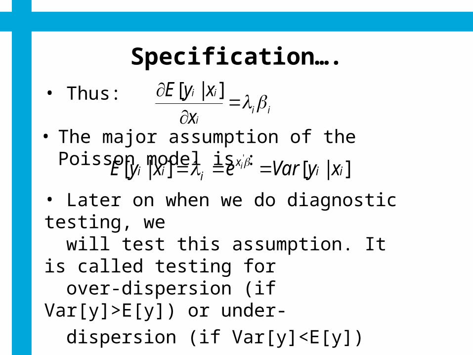
• The major assumption of the Poisson model is :

• Later on when we do diagnostic testing, we will test this assumption. It is called testing for over-dispersion (if Var[y]>E[y]) or under- dispersion (if Var[y]<E[y])

• Thus:ii

i

ii

xxyE

]|[

]|[]|['

iix

iii xyVarexyE i

Estimation• We estimate the model using MLE. The

Likelihood function is non linear:

• The parameters of this equation can be estimated using maximum likelihood method

• Note that the log-likelihood function is concave in and has a unique maxima. (Gourieroux[1991])

n

iiii

n

iiiii yxyeyxyL i

1

'

1

' ]!ln[]!ln[ln'

x

0]][['

1

i

n

ii yeL

i

xx

Estimation….• The Hessian of this function is:

• From this, we can get the asymptotic variance- covariance matrix of the ML estimator:

• Finally, we use the Newton-Raphson iteration to find the parameter estimates:

)()(1

)()1( iiii gH

]['

'

1

'2

ieLH

n

iii

xxx

1

1

' ]][[)ˆ(var'

ien

iiiasy

xxx

Interpretation of the coefficients• Once we obtain the parameter estimates, i.e.

estimates , we can calculate the conditional mean:

Which gives us the expected number of eventsper period.• Further, if xik is the log of an economic variable,

i.e. xik = logXki, can be interpreted as an elasticity

ik

iik X

yElog

][logˆ

ik

'iei

x

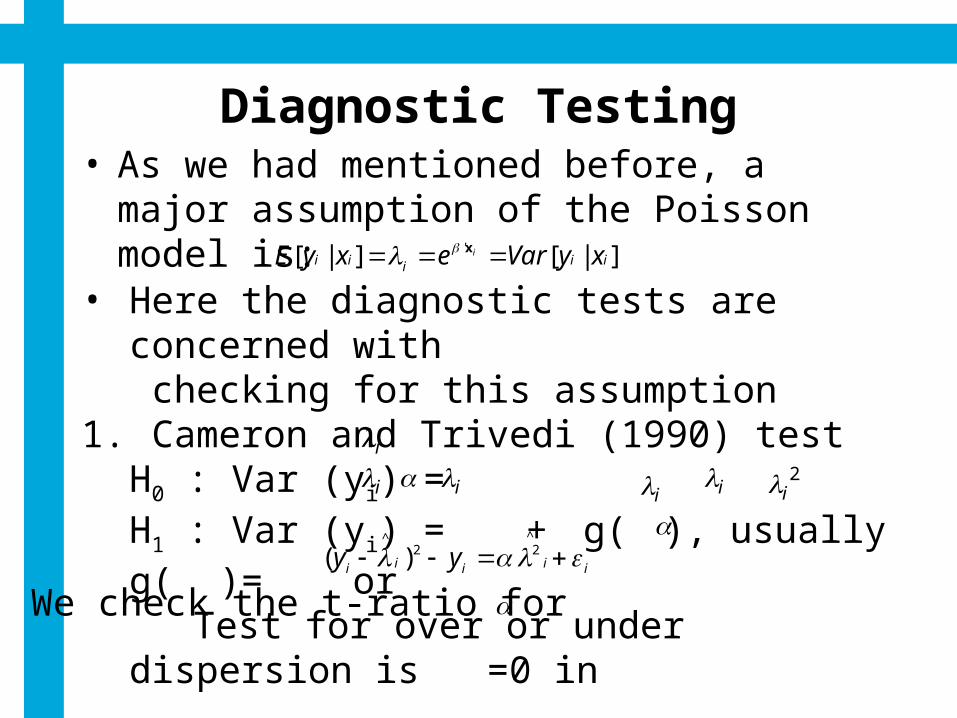
Diagnostic Testing• As we had mentioned before, a major assumption

of the Poisson model is:]|[]|[ '

iiiii xyVarexyE i x

• Here the diagnostic tests are concerned with checking for this assumption

1. Cameron and Trivedi (1990) test H0 : Var (yi) = H1 : Var (yi) = + g( ), usually g( )= or

Test for over or under dispersion is =0 iniiiii yy

^22

^

)(

We check the t-ratio for

i

i ii i 2

i

Diagnostic Testing…• An alternative approach is by Wooldridge(1996)

which involves regressing the square of standardized residuals-1 on the forecasted value and testing alpha = 0 in the following test equation

ii

i

iiy

1)( 2

• In case of miss-specification, we can compute QMLestimators, which are robust – they are consistent estimates as long as the conditional mean in correctlyspecified, even if the distribution is incorrectlyspecified.

Diagnostic Testing…• With miss-specification, the std errors will not be

consistent. We can compute robust std errors using Huber/White (QML) option or GLM , which corrects the std errors for miss-specification.

• For Poisson, MLE are also QMLE• The respective std errors are:

n

ii

ii

MLGLM

yKN 1

22

2

)(1

)(var)(var

Where,

And,

1'

1

ˆˆ)(var

HggHi

iiQML

Empirical Examples

Done in Eviews