An EM Algorithm for Multivariate Mixed Poisson Regression ... · An EM algorithm for multivariate...

Applied Mathematical Sciences, Vol. 6, 2012, no. 137, 6843 - 6856

An EM Algorithm for Multivariate Mixed Poisson

Regression Models and its Application

M. E. Ghitany1, D. Karlis2, D.K. Al-Mutairi1 and F. A. Al-Awadhi1

1Department of Statistics and Operations ResearchFaculty of Science, Kuwait University, Kuwait

2Department of StatisticsAthens University of Economics, Greece

Abstract

Although the literature on univariate count regression models allow-ing for overdispersion is huge, there are few multivariate count regressionmodels allowing for correlation and overdiseprsion. The latter modelscan find applications in several disciplines such as epidemiology, mar-keting, sports statistics, criminology, just to name a few. In this paper,we propose a general EM algorithm to facilitate maximum likelihoodestimation for a class of multivariate mixed Poisson regression models.We give special emphasis to the multivariate negative binomial, Poissoninverse Gaussian and Poisson lognormal regression models. An applica-tion to a real dataset is also given to illustrate the use of the proposedEM algorithm to the considered multivariate regression models.

Mathematics Subject Classification: 62J05, 65D15

Keywords: Mixed Poisson distributions, overdispersion, covariates, EMalgorithm

1 Introduction

Count data occur in several different disciplines. When only one count vari-able is considered the literature is vast. There are various models to fit suchdata and to make inferences on them. For example, traditionally one mayuse the simple Poisson distribution or extensions like mixed Poisson modelswhich allow for overdispersion in the data (sample variance exceeds the samplemean). When considering jointly two or more count variables, things are morecomplicated and the literature is much smaller. Modeling correlated count

6844 M.E. Ghitany, D. Karlis, D.K. Al-Mutairi and F.A. Al-Awadhi

data is also important in certain disciplines, for example in epidemiology whenmore than one disease is considered or in marketing when purchase frequencyof many items is of interest. In the presence of covariates information, for theunivariate case the researcher has a plethora of models available, but for thecase of multivariate count regression models are less developed.

The kind of models that we will consider in this paper are as follows. Sup-pose we have m independent Poisson random variables, X1, . . . , Xm, withrespective means αθ1, . . . , αθm, where α is a random variable from some mix-ing distribution. In practice, the mixing distribution introduces overdispersion,but since α is common to all the Xj ’s it also introduces correlation. We furtherassume that the parameters θj , j = 1, . . . , m, are connected through a log linkfunction with some covariates, namely

log θj = βTj zj, j = 1, . . . , m,

where βj is a (p + 1)-dimensional vector of regression coefficients and zj is a(p + 1)-dimensional vector of covariates associated with variate Xj. To ensuremodel identifiability, it is customary to assume E(α) = 1.

The literature on this approach contains the works of Stein and Yuritz(1987), Stein et al. (1987) and Kocherlakota (1988) for the case without co-variates. Munkin and Trivedi (1999) described multivariate mixed Poisson re-gression models using a gamma mixing distribution. Gurmu and Elder (2000)used an extended Gamma density as a mixing distribution.

The paper is organized is as follows. In Section 2, we give a detailed de-scription of the proposed multivariate regression models. In Section 3, weconsider gamma, inverse-Gaussian and lognormal mixing distributions, eachwith unit mean, and derive the joint probability mass function (jpmf) of thecorresponding multivariate mixed Poisson regression models. Then, we pro-pose a general EM algorithm to facilitate ML estimation for multivariate mixedPoisson regression models in Section 4. Detailed EM algorithms for the con-sidered multivariate mixed Poisson regression models are given in Section 5.In Section 6, we apply the proposed EM algorithm to a real dataset on thedemand for health care in Australia using the considered multivariate mixedPoisson regression models. Finally, some concluding remarks are given.

2 The model

The multivariate mixed Poisson regression model considered in this paper isdescribed as follows. Let Xij ∼ Poisson(αiθij), i = 1, . . . , n, j = 1, . . . , m,αi are independent and identically distributed (i.i.d) random variables froma mixing distribution with cumulative distribution function (c.d.f.) G(α; φ)where φ is a vector of parameters. To allow for regressors, we let log θij =

An EM algorithm for multivariate mixed Poisson regression models 6845

βTj zij , where

βTj = (β0j , β1j, . . . , βpj), j = 1, 2, . . . , m,

are (p + 1)-dimentional vectors of regression coefficients associated with thej-th variable and

zTij = (1, z1ij, . . . , zpij), i = 1, 2, . . . , n, j = 1, 2, . . . , m,

are (p+1)-dimensional vectors of covariates for the i-th observation related tothe j-th variable.

In the present paper, we consider α as a continuous random variable withsupport on (0,∞). In order to achieve identifiability of the model, we assumethat E(α) = 1. Note that α is considered as a frailty.

The joint probability mass function (jpmf) of the given model (droppingthe observation specific subscript i) is given by

P (x1, . . . , xm; φ) =

∫ ∞

0

m∏j=1

exp(−αθj)(αθj)xj

xj !g(α; φ)dα, (1)

where g(α; φ) is the probability density function (pdf) of α.Some properties associated with the mixed Poisson model given in (1) are

as follows.(i) The marginal distribution of Xj , j = 1, 2, . . . , m, is a mixed Poisson

distribution with the same mixing distribution g(α; ·).(ii) The variance of Xj is

V ar(Xj) = θj (1 + θj σ2),

where σ2 is the variance of α.(iii) The covariance between Xj and Xk is

Cov(Xj, Xk) = θj θk σ2, j �= k.

Since σ2 > 0, the covariance (correlation) is always positive.(iv) The generalized variance ratio (GVR) between a multivariate mixed

Poisson model, i.e. Xj ∼ Poisson(αθj), j = 1, . . . , m, α ∼ G(·; φ) and a simplePoisson model, i.e. Yj ∼ Poisson(θj), j = 1, . . . , m, is given by

GV R =

m∑j=1

V ar(Xj) + 2∑j<k

Cov(Xj, Xk)

m∑j=1

V ar(Yj)= 1 + σ2

m∑j=1

θj .

Note that GV R > 1 for a continuous mixing distribution. Hence, themixing distribution introduces a multivariate overdispersion. Also, the GVRincreases as the variance of the mixing distribution increases.


3 Some multivariate mixed Poisson regression

models

In this section, we consider some multivariate mixed Poisson regression modelsbased on gamma, inverse-Gaussian and log-normal mixing distributions. Thesemodels will be called Multivariate negative binomial, Multivariate Poisson-Inverse Gaussian and Multivariate Poisson-lognormal, respectively.

3.1. Multivariate negative binomialThe negative binomial is traditionally the most widely known and applied

mixed Poisson distribution. So a natural choice for the mixing distribution isto consider a gamma (G) distribution with pdf

g(α; γ) =γγ

Γ(γ)αγ−1 exp(−γα), α, γ > 0,

i.e. a gamma density such that E(α) = 1 and σ2 = 1/γ.The resulting multivariate negative binomial (MNB) distribution has jpmf:

PG(x1, . . . , xm; γ) =

Γ(m∑

j=1

xj + γ)

Γ(γ)m∏

j=1

xj !

γγm∏

j=1

θxj

j

(γ +m∑

j=1

θj)

m�j=1

xj+γ. (2)

To allow for regressors, we assume that log θij = βTj zij.

3.2. Multivariate Poisson-Inverse GaussianThe multivariate Poisson inverse Gaussian (MPIG) model is based on an

inverse Gaussian (IG) mixing distribution with pdf

g(α; δ) =δ√2π

exp(δ2) α−3/2 exp

(−δ2

2

(1

α+ α

)), α, δ > 0.

i.e. an inverse Gaussian distribution such that E(α) = 1 and σ2 = 1/δ2.The resulting MPIG distribution has jpmf:

PIG(x1, . . . , xm; δ) =2δ exp(δ2)√

2πK m�

j=1xj−1/2

(δΔ)

(δ

Δ

) m�j=1

xj−1/2 m∏j=1

θxj

j

xj !, (3)

where Δ =

√δ2 + 2

m∑j=1

θj and Kr(x) denotes the modified Bessel function of

the third kind of order r. To allow for regressors we assume log θij = βTj zij.


Properties of the distribution given in (3) can be found in Stein and Yuritz(1987) and Stein et al. (1987). Our proposed MPIG model generalizes the onein Dean et al. (1989).

Note that both the gamma and IG mixing distributions are special cases ofa larger family of distributions called the Generalized inverse Gaussian (GIG)family of distributions, see Jorgensen (1982), with density function

g(α; λ, γ, δ) =(γ

δ

)λ αλ−1

2Kλ(δγ)exp

(−1

2

(δ2

α+ γ2α

)), α > 0,

where the parameter space is given by

{λ < 0, γ = 0, δ > 0} ∪ {λ > 0, γ > 0, δ = 0} ∪ {−∞ < λ < ∞, γ > 0, δ > 0} .

This distribution will be denoted by GIG(λ, γ, δ).The gamma distribution arises when λ > 0, γ > 0, δ = 0 and the IG

distribution arises when λ = −1/2, γ > 0, δ > 0.

3.3. Multivariate Poisson-lognormalConsider another plausible and commonly used mixing distribution, namely

a log-normal (LN) distribution with density

g(α; ν) =1√

2π ν αexp

(−(log(α) + ν2/2)2

2ν2

), α, ν > 0,

such that E(α) = 1 and σ2 = exp(ν2) − 1.The resulting multivariate Poisson-lognormal (MPLN) has jpmf:

PLN(x1, . . . , xm; ν) =

∫ ∞

0

m∏j=1


xj !

exp(− (log(α)+ν2/2)2

2ν2

)√

2π ν αdα. (4)

Unfortunately, the last integral cannot be simplified and hence numerical in-tegration is needed. To allow for regressors we assume log θij = βT

j zij . TheMPLN distribution given in (4) is different than the one used in Aitchison andHo (1989).

4 General EM algorithm for ML estimation

One of the main obstacles for using multivariate mixed Poisson regression mod-els is that the log-likelihood is complicated and hence its maximization needs aspecial effort. For example, Munkin and Trivedi (1999) used a simulated max-imum likelihood method. In this section, we develop an EM type algorithm


which is easy to use for finding the MLEs of the model’s parameters, since wedo not use derivative based optimization.

The EM algorithm is a powerful algorithm for ML estimation for datacontaining missing values or being considered as containing missing values.This formulation is particularly suitable for distributions arising as mixturessince the mixing operation can be considered as producing missing data. Theunobserved quantities are simply the realizations αi of the unobserved mixingparameter for the i-th observation. Hence at the E-step one needs to calculatethe conditional expectation of some functions of αi’s and then to maximize thelikelihood of the complete model which reduces to maximizing the likelihoodof the mixing density. For more details, see Karlis (2001, 2005). Formally, theEM algorithm can be described as follows:

• E-Step Using the current estimates, say φ(r) taken from the r-th it-eration, calculate the pseudo-values tsi = E(hs(αi) | xi, φ

(r)), for i =1, . . . , n, s = 1, . . . , k, where hs(.) are certain functions.

• M-Step Use the pseudovalues tsi from the E-step to maximize the likeli-hood of the mixing distribution and obtain the updated estimates φ(r+1).

• Iterate between the E-step and the M-step until some convergence crite-rion is satisfied, for example the relative change in log-likelihood betweentwo successive iterations is smaller than 10−8.

For a linear function hs(αi), the conditional posterior expectations can beeasily and accurately obtained as it will be shown in the next section. For morecomplicated functions, if the exact solution is not available, one may proceedeither by appropriate approximations based on Taylor approximations or bynumerical approximations including numerical integration and/or simulationbased approximations. All the above solutions seem to work well in practice.

The M-step is somewhat obvious and depends on the assumed mixing distri-bution. For some distributions a special iterative scheme may be appropriate,and perhaps another EM algorithm.

5 EM algorithm for some multivariate mixed

Poisson regression models

We start this section with a preliminary lemma for calculating positive ornegative moments of the posterior distribution of α | x. These moments willbe very useful for implementing the E-step of the EM algorithm described inSection 4.


Let 1j denote the vector with all entries 0 apart from the j-th entry whichis 1, i.e. 11 = (1, 0, 0, . . . , 0), 12 = (0, 1, 0, . . . , 0) etc.

Lemma 1. Suppose that the vector X = (X1, . . . , Xm) follows a multi-variate mixed Poisson model with jpmf P (x; φ) = P (x1, . . . , xm; φ) given in(1). Then, for r = 1, 2, . . . and j = 1, 2, . . .m,

E(αr | x) =(xj + 1) . . . (xj + r)

θrj

P (x + r1j; φ)

P (x; φ),

and

E(α−r | x) =θr

j

xj(xj − 1) . . . (xj − r + 1)

P (x − r1j ; φ)

P (x; φ), xj �= 0, 1, . . . , r − 1.

Proof. Without loss of generality, we prove the lemma for the case j = 1.The posterior density g(α | x) is given by

g(α | x) =P (x|α) g(α; φ)

P (x; φ).

Thus, for r = 1, 2, . . . , we have

E(αr | x) =

∫ ∞0

αrm∏

j=1

exp(−αθj) (αθj)xj

xj !g(α; φ)dα

P (x; φ)

=

∫ ∞0

(x1+1)...(x1+r) exp(−αθ1)(αθ1)x1+r

θr1 (x1+r)!

m∏j=2


xj !g(α; φ)dα

P (x; φ)

=(x1 + 1) . . . (x1 + r)

θr1

P (x1 + r, x2, . . . , xm; φ)

P (x; φ),

The proof for E(α−r | x) is similar.Note that when xj = 0, 1, . . . , r−1, the negative moments E(α−r | x) must

be calculated individually for each mixing distribution.In order to derive the EM algorithm it is interesting to note that the com-

plete data log-likelihood factors in to two parts. Consider as complete data(Xi1, Xi2, . . . , Xim, αi). i.e. the observed data together with the unobservedvalue of the mixing distribution. Then the complete data log-likelihood takesthe form

�C(Θ) =n∑

i=1

m∑j=1

[−αiθij + xij log(αiθij) − log(xij !)] +n∑

i=1

log(g(αi; φ))


where Θ stands for all the parameters of the model. Clearly, the completedata log-likelihood can be split in two parts. The parameters φ of the mixingdistribution appear only in the second part and thus the expectations needed tobe calculated at the E-step are simply those related to the mixing distributiononly. For estimating parameters φ it suffices to maximize the log-likelihoodof the mixing distribution replacing the unobserved quantities of αi with theirexpectations.

We now describe in detail the EM algorithm for the multivariate mixedPoisson regression models considered in section 3.

5.1. Multivariate negative binomial regression modelFor the gamma mixing distribution, the posterior distribution of α | x is a

gamma distribution with parameters γ +m∑

j=1

xj and γ +m∑

j=1

θj . For the E-step,

we use Lemma 1 or the posterior mean to compute E(α | xi) and we use theposterior distribution to compute E(log αi | xi). The EM-algorithm, in thiscase, is as follows:

• E-Step: Calculate, for all i = 1, 2, . . . , n,

si = E(αi | xi) =

γ +m∑

j=1

xij

γ +m∑

j=1

θij

,

ti = E(log(αi) | xi) = Ψ(γ +m∑

j=1

xij) − log(γ +m∑

j=1

θij),

where Ψ(.) is the digamma function and θij = exp(βTj zij), i = 1, 2, . . . , n, j =

1, 2, . . . , m, are obtained using the current values of βj .

• M-step:

– Update the regression parameters βj, j = 1, 2, . . . , p, using thepseudo-values si as offset values and by fitting a simple Poissonregression model and

– Update γ by

γnew = γold − Ψ(γold) − log(γold) − t̄ + s̄ − 1

Ψ′(γold) − 1/γold

where Ψ′(.) denotes the trigamma function, s̄ and t̄ are the samplemeans of s1, s2, . . . sn and t1, t2, . . . tn, respectively. This is the onestep ahead Newton iteration.


5.2. Multivariate Poisson-inverse Gaussian regression modelFor the IG mixing distribution, the posterior distribution of α | x is a GIG

distribution, namely α | x ∼ GIG(m∑

j=1

xj − 1/2,

√2

m∑j=1

θj + δ2, δ). For the

E-step, we use Lemma 1 to compute E(α | xi) and E(α−1 | xi).The EM-algorithm, in this case, is as follows:For the M-step of the algorithm, we need to derive the expectations of the

form E(α | xi) and E(α−1 | xi) which can be easily derived since we knowthat the density is GIG. Also, simple expectations can be based on Lemma 1.Hence, the EM algorithm is as follows (using the results from Lemma 1).


si = E(αi | xi) =xi1 + 1

θi1

PIG(xi1 + 1, xi2, . . . , xim)

PIG(xi; δ),

ti = E(α−1i | xi) =

⎧⎪⎪⎪⎨⎪⎪⎪⎩

1+δ

�δ2+2

m�j=1

θij

δ2 , if xi = 0,

θij

xij

PIG(xi−1j ;δ)

PIG(xi;δ), if xij > 0,

where θij = exp(βTj zij), i = 1, 2, . . . , n, j = 1, 2, . . . , m, are obtained

using the current values of βj and PIG(xi; δ) is given in (3).

• M-step:

– Update the regression parameters βj, j = 1, 2, . . . , m, using thepseudo-values si as the offset values and by fitting a simple Poissonregression model and

– Update δ by

δnew =1√

s̄ + t̄ − 2.

5.3. Multivariate Poisson-Lognormal regression modelFor the multivariate Poisson log-normal model defined in (4) we can againderive an EM algorithm. However, in this case, since the expectations are noteasy to obtain we may switch to a Monte Carlo EM approach.

The complete data log-likelihood takes the form

�C(Θ) =

n∑i=1

m∑j=1

{−αiθij + xij log(αiθij) − log(xij !)} +

n∑i=1

{−1

2log(π) − log(ν) − log(αi) − (log(αi) + ν2/2)2

2ν2

}.


Thus, the expectations needed for the M-step are E(αi) and E((log αi)2).

Hence the algorithm can be written as


si = E(αi | xi) =(xi1 + 1)

θi1

PLN(xi1 + 1, . . . , xim; ν)

PLN (xi1, . . . , xim; ν),

ti = E((log αi)2 | xi) =

∫ ∞0

(log αi)2∏m

j=1exp(−αiθij)(αiθij)

xij

xij !

exp

�− (log(xij )+ν2/2)2

2ν2

�√

2πναidαi

PLN(xi1, . . . , xim; ν),

Unfortunately, this expectation cannot be simplified. On the other hand,it can be evaluated numerically. Alternatively, a Monte Carlo approachis also possible using a rejection algorithm.

• M-step:

– Update the regression parameters βj, j = 1, 2, . . . , m, using thepseudo-values si as the offset values and by fitting a simple Poissonregression model and

– Update ν by

ν̂new = 2(√

1 + t̄ − 1).

5.4. Computational issuesIn this section, we point out some computational issues related to the imple-mentation of the EM algorithm for the three considered multivariate mixedPoisson regression models.(i) Good starting values for the parameters can be obtained by fitting simpleunivariate Poisson or negative binomial regressions. These will give startingvalues for the regression coefficients. We also emphasize that for the MNBregression model, since the M-step is in fact a Newton-Raphson iteration,one may obtain inadmissible values if the starting values are bad. Hence forthis case the choice of initial values needs special attention. For example, asalready mentioned, α relates to correlation and over-dispersion of the data.Hence, the starting value for the parameter of the mixing distribution maybe chosen by equating the overdispersion of the model to the average of theobserved overdispersion.(ii) The expectations given in Lemma 1 are computationally suitable since thedirect evaluation of the moments sometimes may be more time consuming.Note also that the denominator of each expectation in Lemma 1 is the prob-ability needed for the log-likelihood evaluation and hence in most cases it iseasily available.


(iii) The conditional expectation of α|x itself can be of interest in some appli-cations and is interpreted as a frailty. It represents the ”importance” of eachobservation in the data. An advantage of the algorithm is that this quantityis easily available after completion of the EM algorithm.(iv) The standard errors can be obtained using the standard approach of Louis(1982) for the standard errors for the EM algorithm. Alternatively one canobtain them numerically by the Hessian of the log-likelihood.

6 An Application

We analyze the demand for health care in Australia dataset, first used inCameron and Trivedi (1998). There are 5190 observations. We have used threedependent variables, namely the total number of prescribed medications usedin the past two days (PRESCRIB), the total number of nonprescribed medica-tions used in the past two days (NONPRESC) and the number of consultationswith non-doctor health professionals in the past two weeks (NONDOC). Ascovariates, we used the general health questionnaire score using Goldberg’smethod. The considered covariates are:(i) hscore: (high score indicates bad health),(ii) chcond (chronic condition: 1 if chronic condition(s) but not limited in ac-tivity, 0 other),(iii) sex (1 if female, 0 if male),(iv) age (in years divided by 100),(v) income (annual income in Australian dollars divided by 1000: measured asmid-point of coded ranges).

We have fitted the MNB, MPIG and MPLN regression models using theEM algorithm described in section 5. Standard errors are obtained as usualfrom the EM output. As starting values for all models, we used the regressioncoefficients from separate Poisson regressions and for the overdispersion pa-rameter α, the average of the observed overdispersions. We have checked withother initial values and we always converged to the same solution. For eachmodel, we needed less than 100 iterations. The stopping criterion was to stopiterating when the relative change in the log-likelihood was smaller than 10−8.All computing was made using the statistical computing environment languageR. The MPLN regression model needed more time since we have to evaluatenumerically the integrals. However, even this took less than 3 minutes in anIntel Duo 2Ghz processor. For the other two models, we needed less than 2minutes computing time.

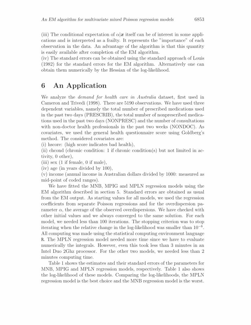
Table 1 shows the estimates and their standard errors of the parameters forMNB, MPIG and MPLN regression models, respectively. Table 1 also showsthe log-likelihood of these models. Comparing the log-likelihoods, the MPLNregression model is the best choice and the MNB regression model is the worst.


MNB MPIG MPLNestimate s.e. estimate s.e. estimate s.e.

PRESCRI (Intercept) -2.245 0.080 -2.275 0.081 -2.290 0.080sex 0.597 0.044 0.618 0.045 0.621 0.044age 2.840 0.107 2.847 0.109 2.859 0.107

income -0.058∗ 0.061 -0.057∗ 0.062 -0.054∗ 0.061hscore 0.121 0.008 0.122 0.008 0.122 0.008chcond 0.389 0.040 0.424 0.041 0.429 0.040

NONPRESCRI (Intercept) -1.328 0.088 -1.347 0.089 -1.361 0.089sex 0.252 0.054 0.267 0.055 0.271 0.055age -0.586 0.139 -0.584 0.141 -0.575 0.141

income 0.265 0.072 0.266 0.073 0.269 0.073hscore 0.083 0.011 0.083 0.011 0.083 0.011chcond 0.268 0.054 0.295 0.054 0.302 0.054

NONDOCO (Intercept) -2.984 0.130 -3.012 0.130 -3.026 0.131sex 0.442 0.073 0.462 0.073 0.466 0.073age 2.169 0.176 2.170 0.177 2.183 0.178

income -0.183∗ 0.104 -0.180∗ 0.105 -0.176∗ 0.105hscore 0.169 0.011 0.170 0.011 0.170 0.012chcond -0.043∗ 0.067 -0.010∗ 0.068 -0.006∗ 0.068

γ̂=1.780 0.090 δ̂=1.227 0.037 ν̂=0.727 0.089loglik -13011.32 -12981.97 -12977.22

Table 1: Results from fitting the three regression models to the demand forhealth care dataset. An * indicates that the test for the regression coefficientis not significant.

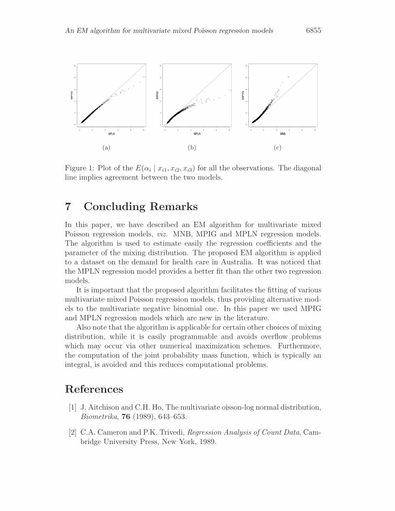
The significance of the covariates was assessed by a Wald type statistic.Recall that the posterior expectation of α for each observation is available

as a byproduct of the EM algorithm. This quantity can be seen as a frailtyimplying the tendency of the patient to need medical treatment. We haveplotted these quantities for any two regression models in Figure 1. Agree-ment between the two models is implied by the diagonal line. Figure 1 showsagreement between the MPIG and MPLN regression models and disagreementbetween these models and the MNB regression model.


0 2 4 6 8 10

02

46

810

MPLN

MP

IG

(a)

0 2 4 6 8 10

02

46

810

MPLN

MN

B

(b)

0 2 4 6 8 10

02

46

810

MNB

MP

IG

(c)

Figure 1: Plot of the E(αi | xi1, xi2, xi3) for all the observations. The diagonalline implies agreement between the two models.

7 Concluding Remarks

In this paper, we have described an EM algorithm for multivariate mixedPoisson regression models, viz. MNB, MPIG and MPLN regression models.The algorithm is used to estimate easily the regression coefficients and theparameter of the mixing distribution. The proposed EM algorithm is appliedto a dataset on the demand for health care in Australia. It was noticed thatthe MPLN regression model provides a better fit than the other two regressionmodels.

It is important that the proposed algorithm facilitates the fitting of variousmultivariate mixed Poisson regression models, thus providing alternative mod-els to the multivariate negative binomial one. In this paper we used MPIGand MPLN regression models which are new in the literature.

Also note that the algorithm is applicable for certain other choices of mixingdistribution, while it is easily programmable and avoids overflow problemswhich may occur via other numerical maximization schemes. Furthermore,the computation of the joint probability mass function, which is typically anintegral, is avoided and this reduces computational problems.

References

[1] J. Aitchison and C.H. Ho, The multivariate oisson-log normal distribution,Biometrika, 76 (1989), 643–653.

[2] C.A. Cameron and P.K. Trivedi, Regression Analysis of Count Data, Cam-bridge University Press, New York, 1989.


[3] C. Dean and J.F. Lawless, A mixed Poisson-inverse Gaussian regressionmodel, Canadian Journal of Statistics, 17 (1989), 171-182.

[4] S. Gurmu and J. Elder, Generalized bivariate Count data regression mod-els, Economics Letters, 68 (2000), 31-36.

[5] B. Jorgensen, Statistical Properties of the Generalized Inverse GaussianDistribution, Lecture Notes in Statistics, Volume 9, Springer-Verlag, NewYork, 1982.

[6] D. Karlis, A general EM approach for maximum likelihood estimation inmixed Poisson regression models, Statistical Modelling, 1 (2001), 305-318.

[7] D. Karlis, An EM algorithm for mixed Poisson distributions, ASTIN Bul-letin, 35 (2005), 3-24.

[8] S. Kocherlakota, On the compounded bivariate Poisson distribution: Aunified treatment, Annals of the Institute of Statistical Mathematics, 40(1988), 61-76.

[9] T.A. Louis, Finding the observed information matrix when using the EMalgorithm, Journal of the Royal Statistical Society B, 44 (1982), 226-233.

[10] M.K. Munkin and P.K. Trivedi, Simulated maximum likelihood estima-tion of multivariate mixed-Poisson regression models, with application,Econometrics Journal, 2 (1999), 29-48.

[11] G. Stein and J.M. Yuritz, Bivariate compound Poisson distributions,Communications in Statistics-Theory and Methods, 16 (1987), 3591-3607.

[12] G.Z. Stein, W. Zucchini and J.M. Juritz, Parameter estimation for theSichel distribution and its multivariate extension, Journal of the AmericanStatistical Association, 82 (1987), 938-944.

Received: March, 2012

An EM Algorithm for Multivariate Mixed Poisson Regression ... · An EM algorithm for multivariate...

Documents

Transcript of An EM Algorithm for Multivariate Mixed Poisson Regression ... · An EM algorithm for multivariate...