Poisson Intensity Estimation withReproducing Kernels

Seth Flaxman, Yee Whye Teh, Dino SejdinovicDepartment of Statistics

University of Oxfordflaxman,y.w.teh,dino.sejdinovic@stats.ox.ac.uk

Abstract

Despite the fundamental nature of the Poisson process in the theory and applicationof stochastic processes, and its attractive generalizations (e.g. Cox process), fewtractable nonparametric modeling approaches exist, especially in multiple dimen-sions. In this paper we develop a new Reproducing Kernel Hilbert Space (RKHS)formulation for the inhomogeneous Poisson process. We model the square root ofthe intensity as an RKHS function. The modeling challenge is that the usual repre-senter theorem arguments no longer apply due to the form of the inhomogeneousPoisson process likelihood. However, we prove that the representer theorem doeshold in an appropriately transformed RKHS, guaranteeing that the optimization ofthe penalized likelihood can be cast as a finite-dimensional problem. The resultingapproach is simple to implement, scales to multiple dimensions and can readily beextended to handle large-scale datasets.

1 Introduction

Poisson processes are ubiquitous in statistical science, with a long history spanning both theory(e.g. [16]) and applications (e.g. [10]), especially in the spatial statistics and time series literature.Despite their ubiquity, fundamental questions in their application to real datasets remain open. Namely,scalable nonparametric models for intensity functions of inhomogeneous Poisson processes are notwell understood, especially in multiple dimensions since the standard approaches are akin to densityestimation. In this contribution, we propose a step towards such scalable nonparametric modelingand introduce a new Reproducing Kernel Hilbert Space (RKHS) formulation for inhomogeneousPoisson process modeling, which is based on the Empirical Risk Minimization (ERM) framework.We model the square root of the intensity as an RKHS function and consider a risk functional givenby a penalized version of the inhomogeneous Poisson process likelihood. While standard representertheorem arguments do not apply directly due to the form of the likelihood—as a counting process,a Poisson process is fundamentally different from standard probability distributions because theobservation that no points occur in some region is just as important as the locations of the pointsthat do occur, and thus the likelihood depends not only on the evaluations of the intensity at theobserved points, but also on its integral across the domain of interest. Nevertheless, we prove aversion of the representer theorem in an appropriately adjusted RKHS. The adjusted RKHS coincideswith the original RKHS as a space of functions but has a different inner product structure. Thisallows us to cast the estimation problem as an optimization over a finite-dimensional subspace ofthe adjusted RKHS. The derived method is demonstrated to give better performance than a naïveunadjusted RKHS method which resorts to an optimization over a subspace without representertheorem guarantees. We describe cases where adjusted RKHS can be described with explicit Mercerexpansions as well as numerical approximations where Mercer expansions are not available. Weobserve strong performance of the proposed method on a variety of synthetic, environmental andbioinformatics data.

2 Background and Related Work

2.1 Poisson process

We briefly state relevant definitions for point processes over domains S ⊂ RD, following [7]. ForLebesgue measurable subsets T ⊂ S, N(T ) denotes the number of events in T ⊂ S. N(·) isa stochastic process characterizing the point process. Our focus is on providing a nonparametricestimator for the first-order intensity of a point process, which is defined as:

λ(s) = lim|ds|→0

E[N(ds))]/|ds| (1)

The inhomogeneous Poisson process is driven solely by the intensity function λ(·):

N(T ) ∼ Poisson(

∫T

λ(x)dx) (2)

In the homogeneous Poisson process, λ(x) = λ is constant, so the number of points in any region Tsimply depends on the volume of T , which we denote |T |:

N(T ) ∼ Poisson(λ|T |) (3)

Assuming that λ(x) is known (either deterministically parameterized with known parameters or ifwe are in a hierarchical model like the Cox process, then conditional on a realization), we havethe following likelihood function for a set of N = N(S) points x1, . . . , xN observed over a fixedwindow S:

L(x1, . . . , xN |λ(x)) =

N∏i=1

λ(xi)exp(−∫S

λ(x)dx

)(4)

2.2 Reproducing Kernel Hilbert Spaces

Given a non-empty domain S and a positive definite kernel function k : S × S → R, thereexists a unique reproducing kernel Hilbert space (RKHS) Hk. RKHS is a space of functionsf : S → R where evaluation is a continuous functional, and can thus be represented by an innerproduct f(x) = 〈f, k(x, ·)〉Hk

for all f ∈ Hk, x ∈ S (reproducing property). While Hk is in mostinteresting cases an infinite-dimensional space of functions, due to the classical representer theorem[15], [24, Section 4.2], optimization overHk is typically a tractable finite-dimensional problem. Inparticular, if we have a set of N observations x1, . . . , xN , xi ∈ S and consider the problem

minf∈Hk

R (f(x1), . . . , f(xN )) + Ω (‖f‖Hk) . (5)

where R (f(x1), . . . , f(xN )) depends on f through its evaluations on the set of observations only,and Ω is a non-decreasing function of the RKHS norm of f , there exists a solution to Eq. (5) ofthe form f∗(·) =

∑Ni=1 αik(xi, ·), and the optimization can thus be cast in terms of α ∈ RN . This

formulation is widely used in the framework of regularized Empirical Risk Minimization (ERM)for supervised learning, where R (f(x1), . . . , f(xN )) = 1

N

∑Ni=1 L(f(xi), yi) is the empirical risk

corresponding to a loss function L.

If domain S is compact and kernel k is continuous, one can assign to k its integral kernel operatorTk : L2(S) → L2(S), given by Tkg =

∫Sk(x, ·)g(x)dx, which is positive, self-adjoint and

compact. There thus exists an orthonormal set of eigenfunctions ej∞j=1 of Tk, and the correspondingeigenvalues ηj∞j=1. This spectral decomposition of Tk leads to Mercer’s representation of kernelfunction k [24, Section 2.2]:

k(x, x′) =

∞∑j=1

ηjej(x)ej(x′), x, x′ ∈ S (6)

with uniform convergence on S × S. Any function f ∈ Hk can then be written as f =∑j bjej

where ‖f‖2Hk=∑j b

2j/ηj <∞.

2

2.3 Related work

The classic approach to nonparametric intensity estimation is based on smoothing kernels [22, 9] andhas a form closely related to the kernel density estimator:

λ(x) =

N∑i=1

k(xi − x) (7)

where k is a smoothing kernel, that is, any bounded function integrating to 1. Early work in this areafocused on edge-corrections and methods for choosing the bandwidth [9, 5, 6]. Connections withRKHS have been considered by, for example, [4] who use a maximum penalized likelihood approachbased on Hilbert spaces to estimate the intensity of a Poisson process. There is long literature onmaximum penalized likelihood approaches to density estimation, which also contain interestingconnections with RKHS, e.g. [25].

Much recent work on estimating intensities for point processes has focused on Bayesian approachesto modeling Cox processes. The log Gaussian Cox Process [20] and related parameterizations of Cox(doubly stochastic) Poisson processes in terms of Gaussian processes have been proposed, along withMonte Carlo [1, 10, 26], Laplace approximate [14, 8, 12] and variational [18, 17] inference schemes.

3 Proposed Method and Kernel Transformation

Let S be a compact domain of observations, e.g. the interval [0, T ] for a time series dataset observedbetween times 0 and T . Let k : S × S → R be a continuous positive definite kernel, and Hkits corresponding RKHS of functions f : S → R. We wish to parameterize the intensity of aninhomogeneous Poisson process using a function f ∈ Hk. We define our intensity as:

λ(x) := af2(x), x ∈ S. (8)where a > 0 is a scale parameter and we have squared f to ensure that the intensity is non-negativeon S. The exact rationale for including a will become clear later—the intuition is that it allows us todecouple the overall scale of the intensity (which depends on the units of the problem, e.g. number ofpoints per hour versus number of points per year) from the penalty on the complexity of f whicharises from the classical regularized Empirical Risk Minimization framework (and which shoulddepend only on how complex, i.e. “wiggly” f is).

We use the inhomogeneous Poisson process likelihood from Eq. (4) to write the log-likelihood of aPoisson process corresponding to the observations x1, . . . , xN, for xi ∈ S, and intensity λ(·):

`(x1, . . . , xN |λ) =

N∑i=1

log(λ(xi))−∫S

λ(x)dx (9)

We will consider the problem of minimization of the penalized negative log likelihood, where theregularization term corresponds to the squared Hilbert space norm of f in parametrization Eq. (8):

minf∈Hk

−

N∑i=1

log(af2(xi)) + a

∫S

f2(x)dx+ γ‖f‖2Hk

. (10)

This objective is akin to a classical regularized empirical risk minimization framework over RKHS:there is a term that depends on evaluations of f at the observed points x1, . . . , xN as well as a termcorresponding to the RKHS norm. However, the representer theorem does not apply directly toEq. (10), since there is also a term given by the L2-norm of f , and so there is no guarantee thatthere is a solution of Eq. (10) that lies in spank(xi, ·). We will show that Eq. (10) fortunately stillreduces to a finite-dimensional optimization problem corresponding to a different kernel function kwhich we define below.

Using the Mercer expansion of k in Eq. (6), we can write the objective Eq. (10) as follows:

J [f ] = −N∑i=1

log(af2(xi)) + a‖f‖2L2(S)+ γ‖f‖2Hk

(11)

= −N∑i=1

log(af2(xi)) + a

∞∑j=1

b2j + γ

∞∑j=1

b2jηj. (12)

3

The last two terms can now be merged together, giving

a

∞∑j=1

b2j + γ

∞∑j=1

b2jej

=

∞∑j=1

b2jaηj + γ

ηj=

∞∑j=1

b2jηj(aηj + γ)−1

. (13)

Now, if we define kernel k to be the kernel corresponding to the integral operator Tk := Tk(aTk +

γI)−1, i.e., k is given by:

k(x, x′) =

∞∑j=1

ηjaηj + γ

ej(x)ej(x′), x, x′ ∈ S, (14)

we see that:

J [f ] = −N∑i=1

log(af2(xi)) + ‖f‖2Hk. (15)

We are now ready to state the representer theorem in terms of kernel k.

Theorem 1. There exists a solution of minf∈Hk

−∑Ni=1 log(af2(xi)) + a

∫Sf2(x)dx+ γ‖f‖2Hk

for observations x1, . . . , xN , which takes the form f∗(·) =

∑Ni=1 αik(xi, ·).

Proof. Since∑j

b2jηj<∞ if and only if

∑j

b2jηj(aηj+γ)−1 <∞, i.e. f ∈ Hk ⇐⇒ f ∈ Hk, we have

that the two spaces correspond to exactly the same set of functions. Optimization overHk is thereforeequivalent to optimization over Hk. The proof now follows by applying the classical representertheorem in k to the representation of the objective function in Eq. (15). For completeness, this isgiven in Appendix C.

Remark 1. The notions of the inner product in Hk and Hk are different and thus in generalspank(xi, ·) 6= spank(xi, ·).Remark 2. Notice that unlike in a standard ERM setting, γ = 0 does not recover the unpenalizedrisk, because γ appears in k. Notice further that the overall scale parameter a also appears in k. Thisis important in practice, because it allows us to decouple the scale of the intensity (which is controlledby a) from its complexity (which is controlled by γ).

Illustration. The eigenspectrum of k where k is a squared exponential kernel is shown be-low for various settings of a and γ. Reminiscent of spectral filtering, we see that dependingon the settings of a and γ, eigenvalues are shrunk or inflated as compared to k(x, x′) whichis shown in black. On the right, the values of k(0, x) are shown for the same set of kernels.

2 4 6 8 10

020

4060

80

rank

eige

nval

ue

k(x,x')a = 1, γ = 1 a = 2, γ = 1 a = 5, γ = 1 a = 1, γ = .1 a = 1, γ = .2 a = 1, γ = 5

0.0 0.1 0.2 0.3 0.4 0.5 0.6

01

23

4

x

valu

e of

ker

nel

4 Computation of k

In this section, we consider first the case in which an explicit Mercer expansion is known, andthen we consider the more commonly encountered situation in which we only have access to theparametric form of the kernel k(x, x′), so we must approximate k. We show experimentally that ourapproximation is very accurate by considering the Sobolev kernel, which can be expressed in bothways.

4

4.1 Explicit Mercer Expansion

We start by assuming that we have a kernel k with an explicit Mercer expansion, so we haveeigenvectors ej(x)j∈J and eigenvalues ηjj∈J :

k(x, x′) =∑j∈J

ηjej(x)ej(x′), (16)

with an at most countable index set J . Given a and γ we can calculate:

k(x, x′) =∑j∈J

ηjaηj + γ

ej(x)ej(x′) (17)

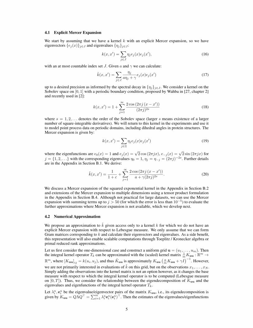
up to a desired precision as informed by the spectral decay in ηjj∈J . We consider a kernel on theSobolev space on [0, 1] with a periodic boundary condition, proposed by Wahba in [27, chapter 2]and recently used in [2]:

k(x, x′) = 1 +

∞∑j=1

2 cos (2πj (x− x′))(2πj)2s

(18)

where s = 1, 2, . . . denotes the order of the Sobolev space (larger s means existence of a largernumber of square-integrable derivatives). We will return to this kernel in the experiments and use itto model point process data on periodic domains, including dihedral angles in protein structures. TheMercer expansion is given by:

k(x, x′) =∑j∈Z

ηjej(x)ej(x′) (19)

where the eigenfunctions are e0(x) = 1 and ej(x) =√

2 cos (2πjx), e−j(x) =√

2 sin (2πjx) forj = 1, 2, . . . with the corresponding eigenvalues η0 = 1, ηj = η−j = (2πj)−2s. Further detailsare in the Appendix in Section B.1. We derive:

k(x, x′) =1

1 + c+

∞∑j=1

2 cos (2πj (x− x′))a+ γ(2πj)2s

. (20)

We discuss a Mercer expansion of the squared exponential kernel in the Appendix in Section B.2and extensions of the Mercer expansion to multiple dimensions using a tensor product formulationin the Appendix in Section B.4. Although not practical for large datasets, we can use the Mercerexpansion with summing terms up to j > 50 (for which the error is less than 10−5) to evaluate thefurther approximations where Mercer expansion is not available, which we develop next.

4.2 Numerical Approximation

We propose an approximation to k given access only to a kernel k for which we do not have anexplicit Mercer expansion with respect to Lebesgue measure. We only assume that we can formGram matrices corresponding to k and calculate their eigenvectors and eigenvalues. As a side benefit,this representation will also enable scalable computations through Toeplitz / Kronecker algebra orprimal reduced rank approximations.

Let us first consider the one-dimensional case and construct a uniform grid u = (u1, . . . , um). Thenthe integral kernel operator Tk can be approximated with the (scaled) kernel matrix 1

mKuu : Rm →Rm, where [Kuu]ij = k(ui, uj), and thus Kuu is approximately Kuu

(amKuu + γI

)−1. However,

we are not primarily interested in evaluations of k on this grid, but on the observations x1, . . . , xN .Simply adding the observations into the kernel matrix is not an option however, as it changes the basemeasure with respect to which the integral kernel operator is to be computed (Lebesgue measureon [0, T ]). Thus, we consider the relationship between the eigendecomposition of Kuu and theeigenvalues and eigenfunctions of the integral kernel operator Tk.

Let λui , eui be the eigenvalue/eigenvector pairs of the matrix Kuu, i.e., its eigendecomposition is

given by Kuu = QΛQ> =∑mi=1 λ

ui eui (eui )>. Then the estimates of the eigenvalues/eigenfunctions

5

of the integral operator Tk are given by the Nyström method (see [23, Section 4.3] and referencestherein, especially [3]):

ηi =1

mλui , ei(x) =

√m

λuiKxue

ui , (21)

with Kxu = [k(x, u1), . . . , k(x, um)], leading to:k(x, x′) =

m∑i=1

ηiaηi + γ

ei(x)ei(x′) =

m∑i=1

1mλ

ui

amλ

ui + γ

· m

(λui )2Kxue

ui (eui )>Kux′ (22)

= Kxu

m∑i=1

1(amλ

ui + γ

)λui

eui (eui )>

Kux′ . (23)

For an estimate of the whole matrix Kxx we thus haveKxx = Kxu

m∑i=1

1(amλ

ui + γ

)λui

eui (eui )>

Kux = KxuQ

( am

Λ2 + γΛ)−1

Q>Kux. (24)

The above is reminiscent of the Nyström method [28] proposed for speeding up Gaussian processregression. A reduced rank representation for Eq. (24) is straightforward by considering only thetop p eigenvalues/eigenvectors of Kuu. Computational cost is thus O(m3 +N2m). Furthermore, aprimal representation with the features corresponding to kernel k is readily available and is given by

φ(x) =( am

Λ2 + γΛ)−1/2

Q>Kux, (25)

which allows linear computational cost in the number N of observations.

For D > 1 dimensions, one can exploit Kronecker and Toeplitz algebra approaches. Assuming thatthe Kuu matrix corresponds to a Cartesian product structure of the one-dimensional grids of sizem, one can write Kuu = K1 ⊗K2 · · · ⊗KD. Thus, the eigenspectrum can be efficiently calculatedby eigendecomposing each of the smaller m×m matrices K1, . . . ,KD and then applying standardKronecker algebra, thereby avoiding ever having to form the prohibitively large mD ×mD matrixKuu. For regular grids and stationary kernels, each small matrix will be Toeplitz structured, yieldingfurther efficiency gains [29]. The resulting approach therefore scales linearly in dimension D.

We compared the exact calculation of Kuu with s = 1, a = 10, and γ = .5 to our approximatecalculation. For illustration we tried a coarse grid of size 10 on the unit interval (left) to a finergrid of size 100. The RMSE was 2E-3 for the coarse grid and 1.6E-5 for the fine grid, as shownin the Appendix in Figure A4. In the same figure we compared the exact calculation of Kxx withs = 1, a = 10, and γ = .5 to our Nyström-based approximation, where x1, . . . , x400 ∼ Beta(.5, .5)distribution. The RMSE was 0.98E-3. A low-rank approximation using only the top 5 eigenvaluesgives the RMSE of 1.6E-2.

5 Inference

The penalized risk can be readily minimized with gradient descent. Let α = [α1, . . . , αN ]> and K bethe Gram matrix corresponding to k such that Kij = k(xi, xj). Then [f(x1), . . . , f(xN )]> = Kαand the gradient of the objective function J from (15) is calculated as follows, where log(·) isunderstood to be applied element-wise to a vector.

∇αJ = −∇α∑i

log(af2(xi)) + γ∇α‖f‖2Hk= −∇α

∑i

log(a(∑j

kijαj)2) + γ∇αα>Kα

= −∑i

2a(∑j kijαj)∇α

∑j kijαj

a(∑j kijαj)

2+ 2γKα = −

∑i

2K·i∑j kijαj

+ 2γKα

= −2∑i

(K·i./(Kα)) + 2γKα

where ./ denotes element-wise division. We use L-BFGS-B to maximize R. Computing K requiresO(N2) time and memory, and each gradient and likelihood computation requires matrix-vector

6

multiplications which are also O(N2). Overall, the running time is O(qN2) for q iterations of thegradient descent method, where q is usually very small in practice.

6 Naïve RKHS model

In this section, we compare the proposed approach, which uses the representer theorem in the trans-formed kernel k, to the naïve one, where a solution to Eq. (10) of the form f(·) =

∑Nj=1 αjk(xj , ·)

is sought even though the representer theorem in k need not hold. Despite being theoretically subopti-mal, this is a natural model to consider, and it might perform well in practice. The correspondingoptimization problem is:

minf∈spank(xi,·)

−

N∑i=1

log(af2(xi)) + a

∫S

f2(x)dx+ γ‖f‖2Hk

. (26)

While the first and the last term are straightforward to calculate for any f(·) =∑j αjk(xj , ·),∫

Sf2(x)dx needs to be estimated. As before, we construct a uniform grid of fineness h, u =

(u1, . . . , un) covering the domain. Then∫S

f2(u)du =

∫S

(α>Kxu

)2du = α>

∫S

KxuKuxdu

α ≈ hα>KxuKuxα, (27)

and the optimization problem reads:

minα∈RN

−

N∑i=1

log(a(α>Kxxi)2) + α> (ahKxuKux + γKxx)α

. (28)

We carried out a small simulation study using simulated intensities drawn fromHk where k was thesquared exponential (SE) kernel in order to compare the performance of the correct model using k aspreviously developed to the naïve model discussed above. In both cases we used crossvalidation totune the hyperparameters on the same synthetic dataset. For testing, we calculated the RMSE of eachmethod in reconstructing the true underlying intensity. In 97 out of 100 repetitions, the correct modelhad a smaller average test log-likelihood than the incorrect model (paired t-test p-value < 0.001). Wereport further comparisons in the next section.

7 Experiments

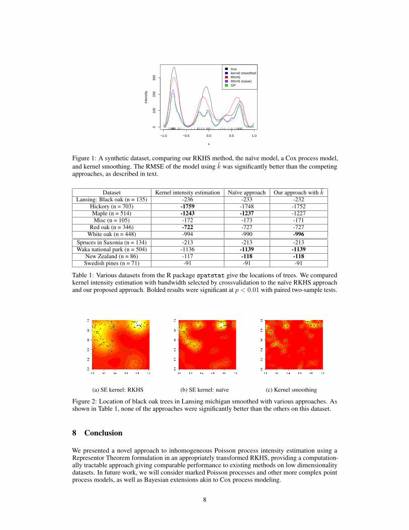
Synthetic Example. We generated a synthetic intensity using the Mercer expansion of a SE kernelwith lengthscale 0.5, producing a random linear combination of 64 basis functions, weighted withiid draws α ∼ N (0, 1). In Figure 1 we compare ground truth to estimates made with: our RKHSmethod with SE kernel, the naïve RKHS approach with SE kernel, a log-Gaussian Cox processmethod [13], and classical kernel smoothing with bandwidth selected by crossvalidation (bw.ucv inR). The RMSE of our method was 34 which compared to 75 for kernel intensity estimation, 75 forthe Cox process, and 86 for the naïve RKHS approach.

Environmental datasets. Next we demonstrate our method on a collection of two-dimensionalenvironmental datasets giving the locations of trees. The datasets were obtained from the R packagespatstat. For illustration, we visualize the locations and intensity estimates for black oak treesin Lansing, Michigan in Figure 2, where we calculated the intensity using various approaches: ourproposed method with squared exponential kernel, our naïve RKHS method with squared exponentialkernel, and classical kernel intensity estimation, with a crossvalidated bandwidth and edge correction.We used cross-validation to tune our methods and we provide cross-validated likelihoods in Table 1.

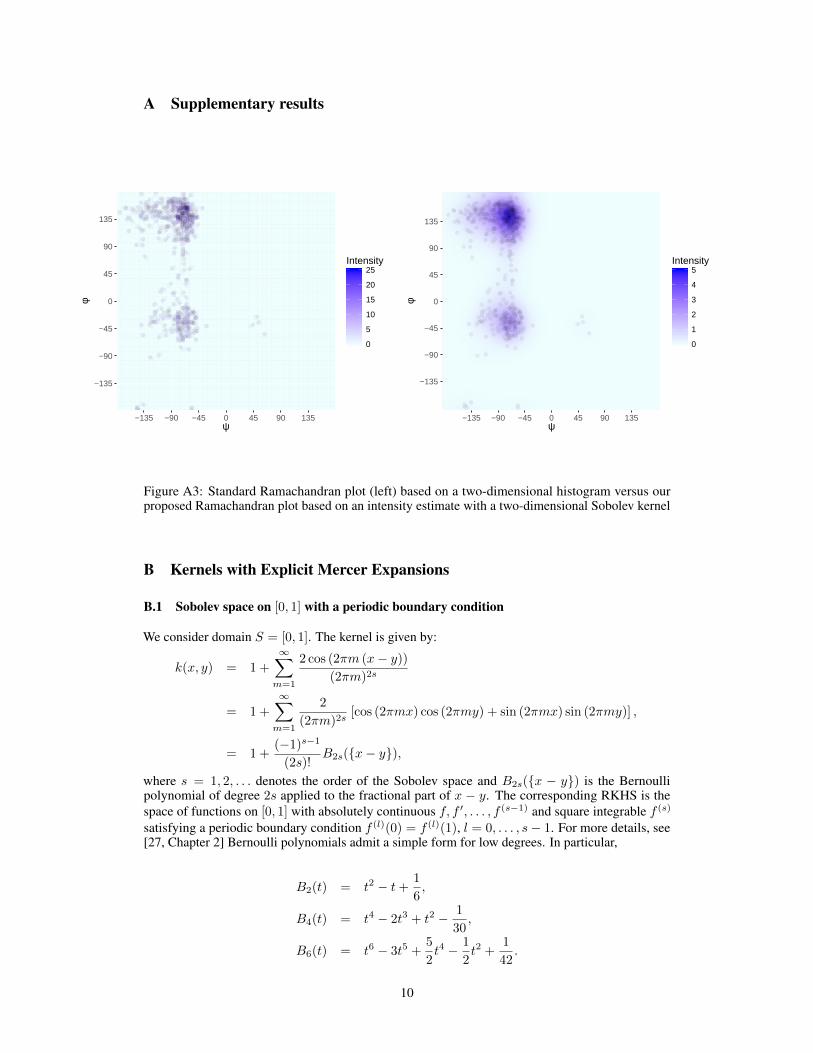
Dihedral angles as point process on a torus. Finally, we consider a novel application of Poissonprocess estimation, suited to our periodic Sobolev kernel. The tensor product construction in twodimensions is appropriate for data observed on a torus. An example from protein bioinformatics isshown in Figure A3 using data included with the R package MDplot, visualizing the dihedral torsionangles [ψ, φ] of amino acids in proteins [21, 19]. Classically, datasets of observed angle pairs havebeen binned using two-dimensional histograms. We propose to treat a set of observed angles as aninhomogeneous Poisson process, enabling intensity estimation as shown.

7

−1.0 −0.5 0.0 0.5 1.0

010

020

030

0

xin

tens

ity

truekernel smoothedRKHSRKHS (naive)GP

Figure 1: A synthetic dataset, comparing our RKHS method, the naïve model, a Cox process model,and kernel smoothing. The RMSE of the model using k was significantly better than the competingapproaches, as described in text.

Dataset Kernel intensity estimation Naïve approach Our approach with kLansing: Black oak (n = 135) -236 -233 -232

Hickory (n = 703) -1759 -1748 -1752Maple (n = 514) -1243 -1237 -1227Misc (n = 105) -172 -173 -171

Red oak (n = 346) -722 -727 -727White oak (n = 448) -994 -990 -996

Spruces in Saxonia (n = 134) -213 -213 -213Waka national park (n = 504) -1136 -1139 -1139

New Zealand (n = 86) -117 -118 -118Swedish pines (n = 71) -91 -91 -91

Table 1: Various datasets from the R package spatstat give the locations of trees. We comparedkernel intensity estimation with bandwidth selected by crossvalidation to the naïve RKHS approachand our proposed approach. Bolded results were significant at p < 0.01 with paired two-sample tests.

(a) SE kernel: RKHS (b) SE kernel: naïve (c) Kernel smoothing

Figure 2: Location of black oak trees in Lansing michigan smoothed with various approaches. Asshown in Table 1, none of the approaches were significantly better than the others on this dataset.

8 Conclusion

We presented a novel approach to inhomogeneous Poisson process intensity estimation using aRepresentor Theorem formulation in an appropriately transformed RKHS, providing a computation-ally tractable approach giving comparable performance to existing methods on low dimensionalitydatasets. In future work, we will consider marked Poisson processes and other more complex pointprocess models, as well as Bayesian extensions akin to Cox process modeling.

8

References[1] Adams, R. P., Murray, I., and MacKay, D. J. Tractable nonparametric bayesian inference in poisson

processes with gaussian process intensities. In Proceedings of the 26th Annual International Conferenceon Machine Learning, pages 9–16. ACM, 2009.

[2] Bach, F. On the equivalence between quadrature rules and random features. arXiv:1502.06800, 2015.[3] Baker, C. The Numerical Treatment of Integral Equations. Monographs on Numerical Analysis Series.

Oxford : Clarendon Press, 1977. ISBN 9780198534068.[4] Bartoszynski, R., Brown, B. W., McBride, C. M., and Thompson, J. R. Some nonparametric techniques for

estimating the intensity function of a cancer related nonstationary poisson process. The Annals of Statistics,pages 1050–1060, 1981.

[5] Berman, M. and Diggle, P. Estimating weighted integrals of the second-order intensity of a spatial pointprocess. Journal of the Royal Statistical Society. Series B (Methodological), pages 81–92, 1989.

[6] Brooks, M. M. and Marron, J. S. Asymptotic optimality of the least-squares cross-validation bandwidth forkernel estimates of intensity functions. Stochastic Processes and their Applications, 38(1):157–165, 1991.

[7] Cressie, N. and Wikle, C. Statistics for spatio-temporal data, volume 465. Wiley, 2011.[8] Cunningham, J. P., Shenoy, K. V., and Sahani, M. Fast gaussian process methods for point process intensity

estimation. In ICML, pages 192–199. ACM, 2008.[9] Diggle, P. A kernel method for smoothing point process data. Applied Statistics, pages 138–147, 1985.

[10] Diggle, P. J., Moraga, P., Rowlingson, B., Taylor, B. M., et al. Spatial and spatio-temporal log-gaussiancox processes: extending the geostatistical paradigm. Statistical Science, 28(4):542–563, 2013.

[11] Fasshauer, G. E. and McCourt, M. J. Stable evaluation of gaussian radial basis function interpolants. SIAMJournal on Scientific Computing, 34(2):A737–A762, 2012.

[12] Flaxman, S. R., Wilson, A. G., Neill, D. B., Nickisch, H., and Smola, A. J. Fast Kronecker inference inGaussian processes with non-Gaussian likelihoods. International Conference on Machine Learning, 2015.

[13] Flaxman, S. R., Neill, D. B., and Smola, A. J. Gaussian processes for independence tests with non-iid datain causal inference. ACM Transactions on Intelligent Systems and Technology (TIST), 2016.

[14] Illian, J. B., Sørbye, S. H., Rue, H., et al. A toolbox for fitting complex spatial point process models usingintegrated nested laplace approximation (inla). The Annals of Applied Statistics, 6(4):1499–1530, 2012.

[15] Kimeldorf, G. and Wahba, G. Some results on tchebycheffian spline functions. Journal of MathematicalAnalysis and Applications, 33(1):82 – 95, 1971. ISSN 0022-247X.

[16] Kingman, J. F. C. Poisson processes, volume 3 of Oxford Studies in Probability. The Clarendon PressOxford University Press, New York, 1993. ISBN 0-19-853693-3. Oxford Science Publications.

[17] Kom Samo, Y.-L. and Roberts, S. Scalable nonparametric bayesian inference on point processes withgaussian processes. In ICML, pages 2227–2236, 2015.

[18] Lloyd, C., Gunter, T., Osborne, M., and Roberts, S. Variational inference for gaussian process modulatedpoisson processes. In ICML, pages 1814–1822, 2015.

[19] Mardia, K. V. Statistical approaches to three key challenges in protein structural bioinformatics. Journal ofthe Royal Statistical Society: Series C (Applied Statistics), 62(3):487–514, 2013.

[20] Møller, J., Syversveen, A., and Waagepetersen, R. Log Gaussian Cox processes. Scandinavian Journal ofStatistics, 25(3):451–482, 1998.

[21] Ramachandran, G. N., Ramakrishnan, C., and Sasisekharan, V. Stereochemistry of polypeptide chainconfigurations. Journal of molecular biology, 7(1):95–99, 1963.

[22] Ramlau-Hansen, H. Smoothing counting process intensities by means of kernel functions. Ann. Statist., 11(2):453–466, 06 1983. doi: 10.1214/aos/1176346152.

[23] Rasmussen, C. E. and Williams, C. K. Gaussian processes for machine learning, 2006.[24] Schölkopf, B. and Smola, A. J. Learning with kernels: support vector machines, regularization, optimiza-

tion and beyond. the MIT Press, 2002.[25] Silverman, B. W. On the estimation of a probability density function by the maximum penalized likelihood

method. Ann. Statist., 10(3):795–810, 09 1982. doi: 10.1214/aos/1176345872.[26] Teh, Y. W. and Rao, V. Gaussian process modulated renewal processes. In Advances in Neural Information

Processing Systems, pages 2474–2482, 2011.[27] Wahba, G. Spline models for observational data, volume 59. Siam, 1990.[28] Williams, C. and Seeger, M. Using the nyström method to speed up kernel machines. In Proceedings of

the 14th Annual Conference on Neural Information Processing Systems, pages 682–688, 2001.[29] Wilson, A. G., Dann, C., and Nickisch, H. Thoughts on massively scalable gaussian processes.

arXiv:1511.01870, 2015.[30] Zhu, H., Williams, C. K., Rohwer, R., and Morciniec, M. Gaussian regression and optimal finite dimen-

sional linear models. 1997.

9

A Supplementary results

−135

−90

−45

0

45

90

135

−135 −90 −45 0 45 90 135ψ

φ

0

5

10

15

20

25Intensity

−135

−90

−45

0

45

90

135

−135 −90 −45 0 45 90 135ψ

φ

0

1

2

3

4

5Intensity

Figure A3: Standard Ramachandran plot (left) based on a two-dimensional histogram versus ourproposed Ramachandran plot based on an intensity estimate with a two-dimensional Sobolev kernel

B Kernels with Explicit Mercer Expansions

B.1 Sobolev space on [0, 1] with a periodic boundary condition

We consider domain S = [0, 1]. The kernel is given by:

k(x, y) = 1 +

∞∑m=1

2 cos (2πm (x− y))

(2πm)2s

= 1 +

∞∑m=1

2

(2πm)2s[cos (2πmx) cos (2πmy) + sin (2πmx) sin (2πmy)] ,

= 1 +(−1)s−1

(2s)!B2s(x− y),

where s = 1, 2, . . . denotes the order of the Sobolev space and B2s(x − y) is the Bernoullipolynomial of degree 2s applied to the fractional part of x − y. The corresponding RKHS is thespace of functions on [0, 1] with absolutely continuous f, f ′, . . . , f (s−1) and square integrable f (s)

satisfying a periodic boundary condition f (l)(0) = f (l)(1), l = 0, . . . , s− 1. For more details, see[27, Chapter 2] Bernoulli polynomials admit a simple form for low degrees. In particular,

B2(t) = t2 − t+1

6,

B4(t) = t4 − 2t3 + t2 − 1

30,

B6(t) = t6 − 3t5 +5

2t4 − 1

2t2 +

1

42.

10

If we consider the Mercer expansion where the underlying measure ρ is uniform on [0, 1]: dρ(x) = dx,we have ∫ 1

0

2 cos (2πmx) sin (2πm′x) dx = 0∫ 1

0

2 cos (2πmx) cos (2πm′x) dx = δ(m−m′)∫ 1

0

2 sin (2πmx) sin (2πm′x) dx = δ(m−m′).

Thus, the desired Mercer expansion k(x, y) =∑m∈Z ηmem(x)em(y) has eigenfunctions e0(x) = 1

and for m = 1, 2, . . ., em(x) =√

2 cos (2πmx), e−m(x) =√

2 sin (2πmx) and correspondingeigenvalues η0 = 1, ηm = η−m = (2πm)−2s.

• k(x, y) is the kernel of Tk(Tk + cI)−1 and has form

k(x, y) =∑m∈Z

ηmηm + c

em(x)em(y)

=1

1 + c+

∞∑m=1

2 cos (2πm (x− y))

1 + c(2πm)2s

• To compute∫ 1

0f2(x)dx for f =

∑i αik(·, xi) we have∫ 1

0

f2(x)dx =∑i,j

αiαj

∫ 1

0

k(xi, u)k(u, xj)du

=∑i,j

αiαj∑m,m′

ηmη′m

(ηm + c)(ηm′ + c)em(xi)em′(xj)

∫ 1

0

em(u)em′(u)du

=∑i,j

αiαj∑m

η2m(ηm + c)2

em(xi)em(xj)

= α>Rα,

where kernel matrix R is computed using kernel r of T 2k (Tk + cI)−2, i.e.

r(x, y) =∑m∈Z

η2m(ηm + c)2

em(x)em(y)

=1

(1 + c)2+

∞∑m=1

2 cos (2πm (x− y))

(1 + c(2πm)2s)2.

• To generate a function f ∈ Hk of unit norm ‖f‖Hk= 1, one takes

f(x) = a0 +√

2

M∑m=1

(am cos(2πmx) + a−m sin(2πmx)) , (29)

for which the norm is given by

‖f‖2Hk= a20 +

M∑m=1

(a2m + a2−m)(2πm)2s. (30)

Thus we can simply generate z = (z−M , . . . , z0, . . . , zM ) ∼ N (0, I2M+1), set z = z/‖z‖and then a0 = z0, am = zm(2π|m|)−s, for m 6= 0.

B.2 Squared exponential kernel

A Mercer expansion for the squared exponential kernel was proposed in [30] and refined in [11].However, this expansion is with respect to a Gaussian measure on R, i.e., it consists of eigenfunctionswhich form an orthonormal set in L2(R, ν) where ν = N (0, `2I). The formalism can therefore beused to estimate Poisson intensity functions with respect to such Gaussian measure. In the classical

11

framework, where the intensity is with respect to a Lebesgue measure, numerical approximations ofMercer expansion, as described in Section 4.2 are needed. Following the exposition in [23, section4.3.1] and the relevant errata1 we parameterize the kernel as:

k(x, x′) = exp(−‖x− x′‖2

2σ2) (31)

The Mercer expansion with respect to ν = N (0, `2I) then has the following eigenvalues:

ηi =

√2a

ABi (32)

And eigenfunctions:

ei(x) =1√√a/c 2ii!

exp(−(c− a)x2)Hi(√

2cx) (33)

where Hi is the i-th order (physicist’s) Hermite polynomial, a = 14σ2 , b = 1

2`2 , c =√a2 + 2ab,

A = a+ b+ c, and B = b/A. Thus we have the following eigenvalues for k:

ηi =ηi

aηi + γ=

1

a+ γ√

A2aB

−i(34)

while the eigenfunctions remain the same.

B.3 Brownian Bridge kernel

This is the kernel

k(x, y) = min(x, y)− xy =

∞∑m=1

2 sin(πmx) sin(πmy)

π2m2,

with

ηm =1

π2m2, em(x) =

√2 sin (πmx) , m = 1, 2, . . . . (35)

Thus

k(x, y) =

∞∑m=1

ηmηm + c

em(x)em(y)

=

∞∑m=1

2 sin(πmx) sin(πmy)

1 + cπ2m2

B.4 Extending the Mercer expansion to multiple dimensions

The extension of any kernel to higher dimensions can be constructed by considering tensor productspaces: Hk1⊗k2 (where k1 and k2 could potentially be different kernels with different hyperparame-ters). If k1 has eigenvalues ηi and eigenfunctions ei and k2 has eigenvalues δj and eigenfunctionsfj , then the eigenvalues of the product space are then given by the Cartesian product ηiδj ,∀i, j,and similarly the eigenfunctions are given by ei(x)fj(y). Our regularized kernel has the followingMercer expansion:

k1 ⊗ k2((x, y), (x′, y′)) =∑ij

ηiδjaηiδj + γ

ei(x)ei(x′)fj(y)fj(y

′) (36)

Notice that k1 ⊗ k2 is the kernel corresponding to the integral operator (Tk1⊗Tk2)(aTk1⊗Tk2+γI)−1

which is different than k1 ⊗ k2.

1http://www.gaussianprocess.org/gpml/errata.html

12

C Proof of the Representer Theorem

We decompose f ∈ Hk as the sum of two functions:

f(·) =

N∑j=1

αj k(xj , ·) + v (37)

where v is orthogonal to the span of k(xj , ·)j . We prove that the first term in the objective J [f ]

given in Eq. (15), −∑Ni=1 log(af2(xi)), is independent of v. It depends on f only through the

evaluations f(xi) for all i. Using the reproducing property we have:

f(xi) = 〈f, k(xi, ·)〉 =∑j

αj k(xj , xi) + 〈v, k(xi, ·)〉 =∑j

αj k(xj , xi) (38)

where the last step is by orthogonality. Next we substitute into the regularization term:

γ‖∑j

αj k(xj , ·) + v‖2Hk= γ‖

∑j

αj k(xj , ·)‖2Hk+ ‖v‖2Hk

≥ γ‖∑j

αj k(xj , ·)‖2Hk. (39)

Thus, the choice of v has no effect on the first term in J [f ] and a non-zero v can only increase thesecond term ‖f‖2Hk

, so we conclude that v = 0 and that f∗ =∑Nj=1 αj k(xj , ·) is the minimizer.

D Numerical evaluation of kernel approximations

Here we present an evaluation of the numerical approximation to k described in 4.2 on the case ofthe Sobolev kernel where Mercer expansion is also available so that truncated Mercer expansionrepresentation of k can be treated as a ground truth. As Figure A4, demonstrates, good approximationis possible with a fairly coarse grid u = (u1, . . . , um) as well as with a low-rank approximation.

0.2 0.4 0.6 0.8

0.05

0.10

0.15

0.20

(a)

kern

el v

alue

0.0 0.2 0.4 0.6 0.8 1.0

0.05

0.10

0.15

0.20

(b)

kern

el v

alue

0.0 0.2 0.4 0.6 0.8 1.0

0.05

0.10

0.15

0.20

(c)

kern

el v

alue

0.0 0.2 0.4 0.6 0.8 1.0

0.05

0.10

0.15

0.20

(d)

kern

el v

alue

Figure A4: We compared the exact calculation of Kuu with s = 1, a = 10, and γ = .5 to ourapproximate calculation. For illustration we tried a coarse grid of size 10 on the unit interval (topleft) to a finer grid of size 100 (top right). The RMSE was 2E-3 for the coarse grid and 1.6E-5 forthe fine grid. We compare the exact calculation of Kxx with s = 1, a = 10, and γ = .5 to ourNyström-based approximation, where x1, . . . , x400 ∼ Beta(.5, .5) distribution (bottom left). TheRMSE was 0.98E-3. A low-rank approximation using only the top 5 eigenvalues gives the RMSE of1.6E-2 (bottom right).

13