Dynamic Delegation of Experimentation∗

Yingni Guo†

July, 2014

Abstract

I study a dynamic relationship in which a principal delegates experimentation to an agent.

Experimentation is modeled as a two-armed bandit whose risky arm yields successes following

a Poisson process. Its intensity, unknown to the players, is either high or low. The agent has

private information, his type being his prior belief that the intensity is high. Theagent values

successes more than the principal and therefore prefers to experimentlonger. I show how

to reduce the analysis to a finite-dimensional problem. In the optimal contract, the principal

starts with a calibrated prior belief and updates it as if the agent had no private information.

The agent is free to experiment or not if this belief remains above a cutoff.He is required to

stop once it reaches the cutoff. The cutoff binds for a positive measureof high enough types.

Surprisingly, this delegation rule is time-consistent. I prove that the cutoff rule remains optimal

and time-consistent for more general stochastic processes governing payoffs.

Keywords: principal-agent, delegation, experimentation, two-armed bandit, incomplete

information, no monetary transfers.

JEL Codes: D82, D83, D86.

∗I am grateful to Johannes Hörner, Larry Samuelson and Dirk Bergemann for insightful conversations and constantsupport. I would like to thank Daniel Barron, Alessandro Bonatti, Florian Ederer, Eduardo Faingold, Mitsuru Igami,Yuichiro Kamada, Nicolas Klein, Daniel Kraehmer, Zvika Neeman, Andrew Postlewaite, Andrzej Skrzypacz, PhilippStrack, Eran Shmaya, Juuso Toikka, Juuso Välimäki, Jörgen Weibull, and various seminar and conference audiencesfor insightful discussion and comments.

†Department of Economics, Yale University, 37 Hillhouse Ave., New Haven, CT, 06520, USA,.

1 Introduction

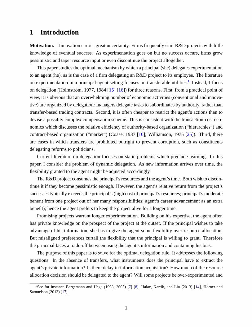
Motivation. Innovation carries great uncertainty. Firms frequently start R&D projects with little

knowledge of eventual success. As experimentation goes on but no success occurs, firms grow

pessimistic and taper resource input or even discontinue the project altogether.

This paper studies the optimal mechanism by which a principal (she) delegates experimentation

to an agent (he), as is the case of a firm delegating an R&D project to its employee. The literature

on experimentation in a principal-agent setting focuses ontransferable utilities.1 Instead, I focus

on delegation (Holmström, 1977, 1984 [15] [16]) for three reasons. First, from a practical point of

view, it is obvious that an overwhelming number of economic activities (conventional and innova-

tive) are organized by delegation: managers delegate tasksto subordinates by authority, rather than

transfer-based trading contracts. Second, it is often cheaper to restrict the agent’s actions than to

devise a possibly complex compensation scheme. This is consistent with the transaction-cost eco-

nomics which discusses the relative efficiency of authority-based organization (“hierarchies”) and

contract-based organization (“market”) (Coase, 1937 [10]; Williamson, 1975 [25]). Third, there

are cases in which transfers are prohibited outright to prevent corruption, such as constituents

delegating reforms to politicians.

Current literature on delegation focuses on static problemswhich preclude learning. In this

paper, I consider the problem of dynamic delegation. As new information arrives over time, the

flexibility granted to the agent might be adjusted accordingly.

The R&D project consumes the principal’s resources and the agent’s time. Both wish to discon-

tinue it if they become pessimistic enough. However, the agent’s relative return from the project’s

successes typically exceeds the principal’s (high cost of principal’s resources; principal’s moderate

benefit from one project out of her many responsibilities; agent’s career advancement as an extra

benefit); hence the agent prefers to keep the project alive for a longer time.

Promising projects warrant longer experimentation. Building on his expertise, the agent often

has private knowledge on the prospect of the project at the outset. If the principal wishes to take

advantage of his information, she has to give the agent some flexibility over resource allocation.

But misaligned preferences curtail the flexibility that the principal is willing to grant. Therefore

the principal faces a trade-off between using the agent’s information and containing his bias.

The purpose of this paper is to solve for the optimal delegation rule. It addresses the following

questions: In the absence of transfers, what instruments does the principal have to extract the

agent’s private information? Is there delay in informationacquisition? How much of the resource

allocation decision should be delegated to the agent? Will some projects be over-experimented and

1See for instance Bergemann and Hege (1998, 2005) [7] [8], Halac, Kartik, and Liu (2013) [14], Hörner andSamuelson (2013) [17].

1

others under-experimented? Is the optimal delegation ruletime-consistent?

Analysis. I examine a dynamic relationship in which a principal delegates experimentation to

an agent. Experimentation is modeled as a continuous-time two-armed bandit problem. See for

instance Presman (1990) [23], Keller, Rady, and Cripps (2005) [20], and Keller and Rady (2010)

[18]. There is one unit of a perfectly divisible resource per unit of time and the agent continually

splits the resource between a safe task and a risky one. In anygiven time interval, the safe task

generates a known flow payoff proportional to the resource allocated to it.2 The risky task’s payoff

depends on an unknown binarystate. In thebenchmark setting, if the state is good the risky task

yieldssuccessesat random times. The arrival rate is proportional to the resource allocated to it. If

the state is bad, the risky task yields no successes. I assumethat the agent values the safe task’s

flow payoffs and the risky task’s successes differently thanthe principal. Both prefer to allocate

the resource to the risky task in the good state and to the safetask in the bad one. However, the

agent values successes relatively more than the principal;hence, he prefers to experiment longer

if faced with prolonged absence of success.3 At the outset, the agent has private information: his

typeis his prior belief that the state is good. After experimentation begins, the agent’s actions and

the arrivals of successes are publicly observed.

The principal delegates the decision on how the agent shouldallocate the resource over time.

This decision is made at the outset. Since the agent has private information before experimentation,

the principal offers a set ofpolicies from which the agent chooses his preferred one. A policy

specifies how the agent should allocate the resource in all future contingencies.

Note that the space of all policies is very large. Possible policies include: allocate all resource

to the risky task until a fixed time and then switch to the safe task only if no success has realized;

gradually reduce the resource input to the risky task if no success occurs and allocate all resource

to it after the first success; allocate all resource to the risky task until the first success and then

allocate a fixed fraction to the risky task; always allocate afixed fraction of the unit resource to the

risky task; etc.

A key observation is that any policy, in terms of payoffs, canbe summarized by a pair of

numbers, corresponding to thetotal expected discounted resourceallocated to the risky task con-

ditional on the state being good and thetotal expected discounted resourceallocated to the risky

task conditional on the state being bad. That is, as far as payoffs are concerned, there is a simple,

finite-dimensional summary statistic for any given policy.The range of these summary statistics

as we vary policies is what I call the feasible set—a subset ofthe plane. Determining the feasible

2The flow payoff generated by the safe task can be regarded as the opportunity cost saved or the payoff fromconducting conventional tasks.

3This assumption will be relaxed later and the case in which the bias goes in the other direction will also be studied.

2

set is a nontrivial problem in general, but it involves no incentive constraints, and so reduces to a

standard optimization problem which I solve. This reduces the delegation problem to a static one.

Given that the problem is now static, I use Lagrangian optimization methods (similar to those used

by Amador, Werning, and Angeletos (2006) [4]) to determine the optimal delegation rule.

Under a mild regularity condition, the optimal delegation rule takes a very simple form. It is a

cutoff rulewith a properly calibrated prior belief that the state is good. This belief is then updated

as if the agent had no private information. In other words, this belief drifts down when no success

is observed and jumps to one upon the first success. It is updated in the way the principal would

if she were carrying out the experiment herself (starting atthe calibrated prior belief). The agent

freely decides whether to experiment or not as long as the updated belief remains above the cutoff.

However, if this belief ever decreases to the cutoff, the agent is required to stop experimenting. This

rule turns out not to bind for types with low enough priors, who voluntarily stop experimenting

conditional on no success, but does constrain those with high enough priors, who are required to

stop when the cutoff is reached.

Given this updating rule, the belief jumps to one upon the first success. Hence, in the bench-

mark setting the cutoff rule can be implemented by imposing adeadline for experimentation, under

which the agent allocates all resource to the risky task after the first success, but is not allowed to

experiment past the deadline. Those types with low enough priors stop experimenting before the

deadline conditional on no success while a positive measureof types with high enough priors stop

at the deadline. In equilibrium, there is no delay in information acquisition as the risky task is

operated exclusively until either the first success revealsthat the state is good or the agent stops.

Among the positive measure of high enough types who are forced to stop when the cutoff (or

the deadline) is reached, the highest subset under-experiment even from the principal’s point of

view. Every other type over-experiments. This implies thatin practice the most promising projects

are always terminated too early while less promising ones are stopped too late due to the agency

problem.

An important property of the cutoff rule is time consistency. After any history the principal

would not adjust the cutoff rule even if she were given a chance to do so. In particular, after the

agent experiments for some time yet no success has realized,the principal still finds it optimal to

keep the cutoff (or the deadline) at the same level as it was set at the beginning. This property

indicates that, surprisingly, implementing the cutoff rule requires minimal commitment on the

principal’s side.

I then show that both the optimality of the cutoff rule and itstime-consistency generalize to

situations in which the risky task generates successes in the bad state as well. When successes

are inconclusive, the belief is updated differently than inthe benchmark setting. It jumps up upon

successes and then drifts down. Consequently, the cutoff rule cannot be implemented by imposing

3

a deadline. Instead, it can be interpreted as asliding deadline. The principal initially extends

some time to the agent to operate the risky task. Then, whenever a success realizes, more time

is extended. The agent is free to switch to the safe task before he uses up the time granted by

the principal. After a long enough period of time elapses without success, the agent is required to

switch to the safe task.

I further extend the analysis to the case in which the agent gains less from the experiment than

the principal and therefore tends to under-experiment. This happens when an innovative task yields

positive externalities, or when it is important to the firm but does not widen the agent’s influence.

When the agent’s bias is small enough, the optimum can be implemented by imposing a lockup

period which is extended upon successes. Instead of placinga cap on the length of experimentation

in the previous case, the principal enacts a floor. The agent has no flexibility but to experiment

before the lockup period ends, yet has full flexibility afterwards. Time-consistency is no longer

valid, though, as whenever the agent stops experimenting voluntarily, he reveals that the principal’s

optimal experimentation length has yet to be reached. The principal is tempted to order the agent

to experiment further. Therefore to implement the sliding lockup period, commitment from the

principal is required.

My results have two important implications for the practical design of delegation rules (I as-

sume a larger agent’s return in this illustration). First, a(sliding) deadline should be in place as a

safeguard against abuse of the principal’s resources. The continuation of the project is permitted

only upon demonstrated successes. Second, the agent shouldhave the flexibility over resource al-

location before the (sliding) deadline is reached. In particular, the agent should be free to terminate

the project whenever he finds appropriate. Besides in-house innovation, these results apply to var-

ious resource allocation problems with experimentation, such as companies budgeting marketing

resources for product introduction and funding agencies awarding grants to scholarly research.4

Related literature. My paper contributes to the literature on delegation. This literature addresses

the incentive problems in organizations which arise due to hidden information and misaligned

preferences. Holmström (1977, 1984) [15] [16] provides conditions for the existence of an optimal

solution to the delegation problem. He also characterizes optimal delegation sets in a series of

examples, under the restriction, for the most part, that only interval delegation sets are allowed.

Alonso and Matouschek (2008) [2] and Amador and Bagwell (2012) [3] characterize the optimal

delegation set in general environments under some conditions and provide conditions under which

simple interval delegation is optimal.

None of these papers consider dynamic delegation. What distinguishes my model from static

4Suppose that experimentation has a flow cost. The agent is cash-constrained and his action is contractible. Dele-gating experimentation equals funding his research project.

4

delegation problems is that additional information arisesover time. The principal ought to use it

both to reduce the agent’s informational rents and to adjusthis behavior. My paper complements

the current literature and facilitates the understanding of how to optimally delegate experimenta-

tion.

Second, my paper is related to the literature on experimentation in a principal-agent setting.5

Since most papers address different issues than I do, here I only mention the most related ones.

Gomes, Gottlieb and Maestri (2013) [13] study a multiple-period model in which the agent has

private information about both the project quality and his cost of effort. The agent’s actions are

observable. Unlike my setting, the agent has no benefit from the project and outcome-contingent

transfers are allowed for. They identify necessary and sufficient conditions under which the prin-

cipal only pays rents for the agent’s information about his cost, but not for the agent’s information

about the project quality. Garfagnini (2011) [12] studies a dynamic delegation model without hid-

den information at the beginning. The principal cannot commit to future actions and transfers are

infeasible. Agency conflicts arise because the agent prefers to work on the project regardless of

the state. He delays information acquisition to prevent theprincipal from growing pessimistic. In

my model, there is pre-contractual hidden information; transfers are infeasible and the principal is

able to commit to long-term contract terms; the agent has direct benefit from experimentation and

shares the same preferences as the principal conditional onthe state. Agency conflicts arise as the

agent is inclined to exaggerate the prospects for success and prolong the experimentation.

The paper is organized as follows. The model is presented in Section2. Section3 considers a

single player’s decision problem. In Section4, I illustrate how to reduce the delegation problem

to a static one. The main results are presented in Section5. I extend the analysis to more general

stochastic processes in Section6 and discuss other applications of the model. Section7 concludes.

2 The model

Players, tasks and states. Time t ∈ [0,∞) is continuous. There are two risk-neutral players

i ∈ α, ρ, an agent (he) and a principal (she), and two tasks, a safe task S and a risky oneR. The

principal is endowed with one unit of perfectly divisible resource per unit of time. She delegates

resource allocation to the agent, who continually splits the resource between the two tasks. The

safe task yields a known deterministic flow payoff that is proportional to the fraction of the resource

5Bergemann and Hege (1998, 2005) [7] [8] study the financing of a new venture in which the principal funds theexperiment and the agent makes contract offers. Dynamic agency problem arises as the agent can invest or divert thefunds. Hörner and Samuelson (2013) [17] consider a similar model in which the agent’s effort requires funding andis unobservable. The principal makes short-term contract offers specifying profit-sharing arrangement. Halac, Kartik,and Liu (2013) [14] study long-term contract for experimentation with adverse selection about the agent’s ability andmoral hazard about his effort choice.

5

allocated to it. The risky task’s payoff depends on an unknown binarystate, ω ∈ 0, 1.

In particular, if the fractionπt ∈ [0, 1] of the resource is allocated toR over an interval[t, t+dt),

and consequently1−πt toS, playeri receives(1−πt)sidt fromS, wheresi > 0 for both players.

The risky task generates asuccessat some point in the interval with probabilityπtλ1dt if ω = 1

and πtλ0dt if ω = 0. Each success is worthhi to player i. Therefore, the overall expected

payoff increment to playeri conditional onω is [(1 − πt)si + πtλωhi]dt. All this data is common

knowledge.6

In the benchmark setting, I assume thatλ1 > λ0 = 0. Hence,R yields no success in state0. In

Subsection6.1.1, I extend the analysis to the setting in whichλ1 > λ0 > 0.

Conflicts of interests. I allow different payoffs to players,i.e., I do not require thatsα = sρ or

hα = hρ. The restriction imposed on payoff parameters is the following:

Assumption 1. Parameters are such thatλ1hi > si > λ0hi for i ∈ α, ρ, and

λ1hα − sαsα − λ0hα

>λ1hρ − sρsρ − λ0hρ

.

Assumption1 has two implications. First, there is agreement on how to allocate the resource if

the state is known. Both players prefer to allocate the resource toR in state1 and the resource toS

in state0. Second, the agent values successes over flow payoffs relatively more than the principal

does. Let

ηi =λ1hi − sisi − λ0hi

denote playeri’s net gain fromR’s successes overS’s flow payoffs. The ratioηα/ηρ, being strictly

greater than one, measures how misaligned players’ interests are and is referred to as the agent’s

bias. (The case in which the bias goes in the other direction is discussed in Subsection6.2.)

Private information. Players do not observe the state. At time0, the agent has private informa-

tion about the probability that the state is1. For ease of exposition, I express the agent’s prior belief

that the state is1 in terms of the implied odds ratio of state1 to state0, denotedθ and referred to

as the agent’s type. The agent’s type is drawn from a compact intervalΘ ≡ [θ, θ] ⊂ R+ according

to some continuous density functionf . LetF denote the cumulative distribution function.

By the definition of the odds ratio, the agent of typeθ assigns probabilityp(θ) = θ/(1 + θ) to

the event that the state is1 at time0. The principal knows only the type distribution. Hence, her

6It is not necessary thatS generates deterministic flow payoffs. What matters to players is that the expected payoffrates ofS are known and equalsi, and thatS’s flow payoffs are uncorrelated with the state.

6

prior belief that the state is1 is given by

E[p(θ)] =

∫

Θ

θ

1 + θdF (θ).

Actions and successes are publicly observable. The only information asymmetry comes from the

agent’s private information about the state at time0. Hence, a resource allocation policy, which I

introduce next, conditions on both the agent’s past actionsand arrivals of successes.

Policies and posterior beliefs. A (pure) resource allocationpolicy is a non-anticipative stochas-

tic processπ = πtt≥0. Here,πt ∈ [0, 1] is interpreted as the fraction of the unit resource allocated

toR at timet, which may depend only on the history of events up tot. A policy π can be described

as follows. At time0, a choice is made of a deterministic functionπ(t | 0), measurable with re-

spect tot, 0 ≤ t < ∞, which takes values in[0, 1] and corresponds to the fraction of the resource

allocated toR up to the moment of the first success. If at the random timeτ1 a success occurs, then

depending on the value ofτ1, a new functionπ(t | τ1, 1) is chosen, etc. The space of all policies,

including randomized ones, is denotedΠ. (See Footnote8.)

LetNt denote the number of successes observed up to timet. Both players discount payoffs at

rater > 0. Playeri’s payoff given an arbitrary policyπ ∈ Π and an arbitrary prior beliefp ∈ [0, 1]

consists of the expected discounted payoffs fromR’s successes and the expected discounted flow

payoffs fromS

Ui(π, p) ≡ E

[∫ ∞

0

re−rt [hidNt + (1− πt) sidt]∣

∣

∣π, p

]

.

Here, the expectation is taken over the stateω and the stochastic processesπ andNt. By the Law of

Iterated Expectations, I can rewrite playeri’s payoff as the discounted sum of the expected payoff

increments

Ui(π, p) = E

[∫ ∞

0

re−rt [(1− πt)si + πtλωhi] dt

∣

∣

∣π, p

]

.

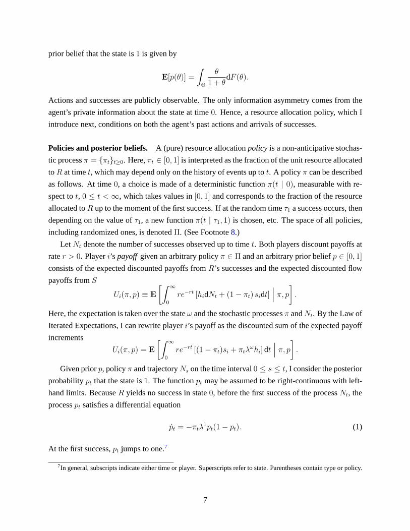
Given priorp, policyπ and trajectoryNs on the time interval0 ≤ s ≤ t, I consider the posterior

probabilitypt that the state is1. The functionpt may be assumed to be right-continuous with left-

hand limits. BecauseR yields no success in state0, before the first success of the processNt, the

processpt satisfies a differential equation

pt = −πtλ1pt(1− pt). (1)

At the first success,pt jumps to one.7

7In general, subscripts indicate either time or player. Superscripts refer to state. Parentheses contain type or policy.

7

Delegation. I consider the situation in which transfers are not allowed and the principal is able

to commit to dynamic policies. At time0, the principal chooses a set of policies from which the

agent chooses his preferred one. Since there is hidden information at time0, by the Revelation

Principle, the principal’s problem is reduced to solving for a mapπ : Θ → Π to maximize her

expected payoff subject to the agent’ incentive compatibility constraint (IC constraint, hereafter).

Formally, I solve

sup

∫

Θ

Uρ(π(θ), p(θ))dF (θ),

subject to Uα(π(θ), p(θ)) ≥ Uα(π(θ′), p(θ)) ∀θ, θ′ ∈ Θ,

over measurableπ : Θ → Π.8

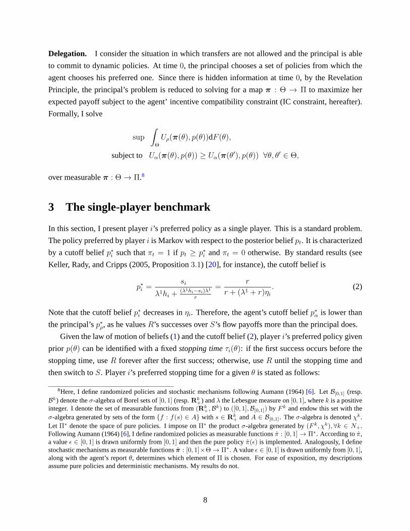
3 The single-player benchmark

In this section, I present playeri’s preferred policy as a single player. This is a standard problem.

The policy preferred by playeri is Markov with respect to the posterior beliefpt. It is characterized

by a cutoff beliefp∗i such thatπt = 1 if pt ≥ p∗i andπt = 0 otherwise. By standard results (see

Keller, Rady, and Cripps (2005, Proposition3.1) [20], for instance), the cutoff belief is

p∗i =si

λ1hi +(λ1hi−si)λ1

r

=r

r + (λ1 + r)ηi. (2)

Note that the cutoff beliefp∗i decreases inηi. Therefore, the agent’s cutoff beliefp∗α is lower than

the principal’sp∗ρ, as he valuesR’s successes overS’s flow payoffs more than the principal does.

Given the law of motion of beliefs (1) and the cutoff belief (2), playeri’s preferred policy given

prior p(θ) can be identified with a fixedstopping timeτi(θ): if the first success occurs before the

stopping time, useR forever after the first success; otherwise, useR until the stopping time and

then switch toS. Playeri’s preferred stopping time for a givenθ is stated as follows:

8Here, I define randomized policies and stochastic mechanisms following Aumann (1964) [6]. Let B[0,1] (resp.Bk) denote theσ-algebra of Borel sets of[0, 1] (resp.Rk

+) andλ the Lebesgue measure on[0, 1], wherek is a positiveinteger. I denote the set of measurable functions from(Rk

+,Bk) to ([0, 1],B[0,1]) by F k and endow this set with theσ-algebra generated by sets of the formf : f(s) ∈ A with s ∈ R

k+ andA ∈ B[0,1]. Theσ-algebra is denotedχk.

Let Π∗ denote the space of pure policies. I impose onΠ∗ the productσ-algebra generated by(F k, χk), ∀k ∈ N+.Following Aumann (1964) [6], I define randomized policies as measurable functionsπ : [0, 1] → Π∗. According toπ,a valueǫ ∈ [0, 1] is drawn uniformly from[0, 1] and then the pure policyπ(ǫ) is implemented. Analogously, I definestochastic mechanisms as measurable functionsπ : [0, 1]×Θ → Π∗. A valueǫ ∈ [0, 1] is drawn uniformly from[0, 1],along with the agent’s reportθ, determines which element ofΠ is chosen. For ease of exposition, my descriptionsassume pure policies and deterministic mechanisms. My results do not.

8

Claim 1. Playeri’s stopping time given odds ratioθ ∈ Θ is

τi(θ) =

1λ1

log (r+λ1)θηir

if (r+λ1)θηir

≥ 1,

0 if (r+λ1)θηir

< 1.

Figure1 illustrates the two players’ cutoff beliefs and their preferred stopping times associated

with two possible odds ratiosθ′, θ′′ (with θ′ < θ′′).9 The prior beliefs are thusp(θ′), p(θ′′) (with

p(θ′) < p(θ′′)). Thex-axis variable is timet and they-axis variable is the posterior belief. On the

y-axis is labeled the two players’ cutoff beliefsp∗ρ andp∗α. The solid and dashed lines depict how

posterior beliefs evolve whenR is used exclusively and no success realizes.

The figure on the left-hand side shows that for a given odds ratio the agent prefers to experiment

longer than the principal does because his cutoff is lower than the principal’s. The figure on the

right-hand side shows that for a given playeri, the stopping time increases in the odds ratio,i.e.,

τi(θ′) < τi(θ

′′). Therefore, both players prefer to experiment longer givena higher odds ratio.

Figure1 makes clear what agency problem the principal faces. The principal’s stopping timeτρ(θ)

is an increasing function ofθ. The agent prefers to stop later than the principal for a given θ and

thus has incentives to misreport his type. More specifically, lower types (those types with a lower

θ) have incentives to mimic high types to prolong the experimentation.

State prob.p

time t

p(θ′)

p∗ρp∗α

τρ(θ′) τα(θ

′)

1

0

State prob.p

time t

p(θ′′)

p(θ′)

p∗ρp∗α

τρ(θ′′)τρ(θ

′) τα(θ′′)τα(θ

′)

1

0

Figure 1: Thresholds and stopping times

Given that a single player’s preferred policy is always characterized by a stopping time, one

might expect that the solution to the delegation problem is aset of stopping times. This is the

case if there is no private information or no bias. For example, if the distributionF is degenerate,

information is symmetric. The optimal delegation set is theprincipal’s preferred stopping time

given her prior. Ifηα/ηρ equals one, the two players’ preferences are perfectly aligned. The

principal, knowing that for any prior the agent’s preferredstopping time coincides with hers, offers

9Parameters in Figure1 areηα = 3/2, ηρ = 3/4, r/λ1 = 1, θ = 3/2, θ′ = 4.

9

the set of her preferred stopping timesτρ(θ) : θ ∈ Θ for the agent to choose from.

However, if the agent has private information and is also biased, it is unclear how the principal

should restrict his actions. Particularly, it is unclear whether the principal would still offer a set of

stopping times. For this reason, I am led to consider the space of all policies.

4 A finite-dimensional characterization of the policy space

The space of all policies is large. In the first half of this section, I associate to each policy—a

(possibly complicated) stochastic process—a pair of numbers, calledtotal expected discounted

resourcepair, and show that this pair is a sufficient statistic for this policy in terms of both players’

payoffs. Then, I solve for the set of feasibletotal expected discounted resourcepairs, which is a

subset ofR2 and can be treated as the space of all policies.

This transformation allows me to reduce the dynamic delegation problem to a static one. In the

second half of this section, I characterize players’ preferences over the feasible pairs and reformu-

late the delegation problem.

4.1 A policy as a pair of numbers

For a fixed policyπ, I definew1(π) andw0(π) as follows:

w1(π) ≡ E

[∫ ∞

0

re−rtπtdt∣

∣

∣π, 1

]

andw0(π) ≡ E

[∫ ∞

0

re−rtπtdt∣

∣

∣π, 0

]

. (3)

The termw1(π) is the expected discounted sum of the resource allocated toR underπ in state1. I

refer tow1(π) as thetotal expected discounted resource(expected resource, hereafter) allocated to

R underπ in state1.10 Similarly, the termw0(π) is theexpected resourceallocated toR underπ

in state0. Bothw1(π) andw0(π) are in[0, 1] becauseπ takes values in[0, 1]. Therefore,(w1,w0)

defines a mapping from the policy spaceΠ to [0, 1]2.

To calculate the payoff of a policy for a given priorp, I first calculate the payoff if the state is1

(or equivalently,p = 1) and the payoff if the state is0 (or equivalently,p = 0). Multiplying these

payoffs by the initial state distribution gives the payoff of this policy. Conditional on the state,

the payoff rate ofR is know and therefore the payoff of a policy is linear in theexpected resource

allocated toR.11 As a result, what is relevant for evaluating a policyπ is itsexpected resourcepair

10For a fixed policyπ, theexpected resourcespent onR in state1 is proportional to the expected discounted numberof successes,i.e., w1(π) = E

[∫∞

0re−rtdNt | π, 1

]

/λ1.11Recall that, conditional on the state and over any interval,S generates a flow payoff proportional to the resource

allocated to it andR yields a success with probability proportional to the resource allocated to it.

10

(w1(π),w0(π)). I summarize this in the following lemma.

Lemma 1 (A policy as a pair of numbers).

For a given policyπ ∈ Π and a given priorp ∈ [0, 1], playeri’s payoff can be written as

Ui(π, p) = p(

λ1hi − si)

w1(π) + (1− p)

(

λ0hi − si)

w0(π) + si. (4)

Proof. Playeri’s payoff given policyπ ∈ Π and priorp ∈ [0, 1] is

Ui(π, p) = E

[∫ ∞

0

re−rt [(1− πt)si + πtλωhi] dt

∣

∣

∣π, p

]

= pE

[∫ ∞

0

re−rt[

si + πt

(

λ1hi − si)]

dt∣

∣

∣π, 1

]

+ (1− p)E

[∫ ∞

0

re−rt[

si + πt

(

λ0hi − si)]

dt∣

∣

∣π, 0

]

= p(

λ1hi − si)

E

[∫ ∞

0

re−rtπtdt∣

∣

∣π, 1

]

+ (1− p)(

λ0hi − si)

E

[∫ ∞

0

re−rtπtdt∣

∣

∣π, 0

]

+ si

= p(

λ1hi − si)

w1(π) + (1− p)

(

λ0hi − si)

w0(π) + si.

Lemma1 shows that(w1(π),w0(π)) is a sufficient statistic for policyπ for the payoffs. Instead

of working with a generic policyπ, it is without loss of generality to focus on(w1(π),w0(π)).

4.2 Feasible set

Let Γ denote the image of the mapping(w1,w0) : Π → [0, 1]2. I call Γ the feasible setsince it

contains all possible(w1, w0) pairs that can be achieved by some policyπ. The following lemma

shows that the feasible set is the convex hull of the image of Markov policies under(w1,w0).

Lemma 2 (Feasible set).

The feasible set is the convex hull of

(w1(π),w0(π)) : π ∈ ΠM

, whereΠM is the set of Markov

policies with respect to the posterior belief of state1.

Proof. The feasible set is convex given that the policy spaceΠ is convexified. (Recall thatΠ in-

cludes all randomized policies (See Footnote8).) Therefore, I only need to characterize its extreme

points. A bundlew is an extreme point ofΓ if and only if there exists(p1, p2) ∈ R2, ‖(p1, p2)‖ = 1

such thatw ∈ arg maxw∈Γ(p1, p2)·w. Therefore, the feasible set can be found by taking the convex

hull of the following set

w ∈ [0, 1]2∣

∣

∣∃(p1, p2) ∈ R

2, ‖(p1, p2)‖ = 1, w ∈ arg maxw∈Γ

(p1, p2) · w

(5)

Comparing the objective(p1, p2) · w with (4), I can rewrite(p1, p2) · w as the expected payoff of

a single playeri whose prior belief of state1 is |p1|/(|p1| + |p2|) and whose payoff parameters

11

aresi = 0, λ1hi = sgn(p1), λ0hi = sgn(p2). Here, sgn(·) is the sign function. It follows that the

argument of the maximum,arg maxw∈Γ(p1, p2) · w, coincides with playeri’s optimal policy. This

transforms the problem to a standard optimization problem.Markov policies are sufficient.

Here, I calculate the image of(w1,w0) for two classes of policies, which turn out to be impor-

tant for characterizingΓ. The first class isstopping-time policies: allocate all resource toR until

a fixed time; if at least one success occurs by then, allocate all resource toR forever; otherwise,

switch toS forever. The image of all stopping-time policies under(w1,w0) is denotedΓst. It is

easy to verify that

Γst =

(

w1, w0)

∣

∣

∣w0 = 1−

(

1− w1)

r

r+λ1 , w1 ∈ [0, 1]

.

The second class isslack-after-success policies: allocate all resource toR until the first success

occurs; then allocate a fixed fraction toR. If the state is0, all resource is directed toR because no

success will occur. The image of all slack-after-success policies under(w1,w0) is denotedΓsl. It

is easy to verify that

Γsl =

(

w1, w0)

∣

∣

∣w0 = 1, w1 ∈

[

r

r + λ1, 1

]

.

The following lemma characterizes the feasible set.

Lemma 3 (Conclusive news—feasible set).

The feasible set is Conv(Γst ∪ Γsl), the convex hull of the image of stopping-time and slack-after-

success policies.

Proof. Based on the proof of Lemma2, I only need to show that the maximum in (5) is achieved

by either a stopping-time or slack-after-success policy. If p1 ≥ 0, p2 ≥ 0 (p1 ≤ 0, p2 ≤ 0),

maxw∈Γ(p1, p2) ·w is achieved by the policy which directs all resources toR (S). If p1 > 0, p2 < 0,

maxw∈Γ(p1, p2) ·w is achieved by a lower-cutoff Markov policy under whichR is used exclusively

if the posterior belief is above the cutoff andS is used below. This Markov policy is effectively a

stopping time policy. Ifp1 < 0, p2 > 0, according to Keller and Rady (2013) [19], maxw∈Γ(p1, p2)·w is achieved by a upper-cutoff Markov policy under whichR is used exclusively if the posterior

belief is below the cutoff andS is used above. This is either a policy allocating all resource toR

until the first success and then switching toS, or a policy allocating all resource toS.

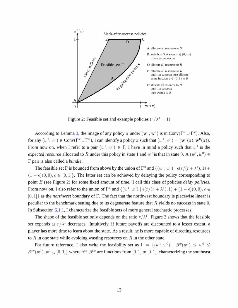
Figure2 depicts the image of all stopping-time policies and slack-after-success policies when

r andλ1 both equal1/5. The shaded area is Conv(Γst ∪ Γsl). The(w1, w0) pairs on the southeast

boundary correspond to stopping-time policies. Those pairs on the north boundary correspond to

slack-after-success policies.

12

w0(π)

w1(π)0 1

1

Feasible set:Γ

Slack-after-success policies

Stopp

ing-

time

polic

ies

Del

aypo

licie

s

A: allocate all resource toS

B: switch toS at someτ ∈ (0,∞)

if no success occurs

C: allocate all resource toR

D: allocate all resource toRuntil 1st success; then allocatesome fractionφ ∈ (0, 1) toR

E: allocate all resource toRuntil 1st success;then switch toS

bA

bB

b Cb

DbE

Figure 2: Feasible set and example policies (r/λ1 = 1)

According to Lemma3, the image of any policyπ under(w1,w0) is in Conv(Γst ∪ Γsl). Also,

for any(w1, w0) ∈ Conv(Γst∪Γsl), I can identify a policyπ such that(w1, w0) = (w1(π),w0(π)).

From now on, when I refer to a pair(w1, w0) ∈ Γ, I have in mind a policy such thatw1 is the

expected resourceallocated toR under this policy in state1 andw0 is that in state0. A (w1, w0) ∈Γ pair is also called abundle.

The feasible setΓ is bounded from above by the union ofΓsl and(w1, w0) | ǫ(r/(r+λ1), 1)+(1 − ǫ)(0, 0), ǫ ∈ [0, 1]. The latter set can be achieved by delaying the policy corresponding to

pointE (see Figure2) for some fixed amount of time. I call this class of policiesdelay policies.

From now on, I also refer to the union ofΓsl and(w1, w0) | ǫ(r/(r + λ1), 1) + (1− ǫ)(0, 0), ǫ ∈[0, 1] as thenorthwestboundary ofΓ. The fact that the northwest boundary is piecewise linear is

peculiar to the benchmark setting due to its degenerate feature thatR yields no success in state0.

In Subsection6.1.1, I characterize the feasible sets of more general stochastic processes.

The shape of the feasible set only depends on the ratior/λ1. Figure3 shows that the feasible

set expands asr/λ1 decreases. Intuitively, if future payoffs are discounted to a lesser extent, a

player has more time to learn about the state. As a result, he is more capable of directing resources

toR in one state while avoiding wasting resources onR in the other state.

For future reference, I also write the feasibility set asΓ = (w1, w0) | βse(w1) ≤ w0 ≤βnw(w1), w1 ∈ [0, 1] whereβse, βnw are functions from[0, 1] to [0, 1], characterizing the southeast

13

w0(π)

w1(π)0 1

1

r/λ1 = 2

r/λ1 = 1

r/λ1 = 1/2

The feasible set expands asr/λ1 decreases.

Figure 3: Feasible sets asr/λ1 varies

and northwest boundaries of the feasible set,

βse(

w1)

≡ 1−(

1− w1)

r

r+λ1 ,

βnw(

w1)

≡

(r + λ1)w1 if w1 ∈[

0, 1r+λ1

]

,

1 if w1 ∈(

1r+λ1

, 1r

]

.

4.3 Preferences over feasible pairs

If a player knew the state, he would allocate all resources toR in state1 and all resources toS in

state0. However, this allocation cannot be achieved if the state isunknown. A policy, being state-

independent, necessarily entails the cost of learning. If aplayer wants to direct more resources to

R in state1, he has to allocate more resources toR before the arrival of the first success. Inevitably,

more resources will be wasted onR if the state is actually0.

A player’s attitude toward this trade-off between spendingmore resources onR in state1 and

wasting less resources onR in state0 depends on how likely the state is1 and how much he gains

from R’s successes overS’s flow payoffs. According to Lemma1, playeri’s payoff given policy

π and odds ratioθ is

Ui(π, p(θ)) =

(

θ

1 + θηiw

1(π)− 1

1 + θw

0(π)

)

(

si − λ0hi)

+ si.

Recall thatp(θ) = θ/(1 + θ) is the prior that the state is1 given θ. Playeri’s preferences over

(w1, w0) are characterized by upward-sloping indifference curves with the slope beingθηi. For a

14

fixed player, the indifference curves are steeper for higherodds ratios. For a fixed odds ratio, the

agent’s indifference curves are steeper than the Principal’s (see Figure4).12 Playeri’s preferred

bundle givenθ, denoted(w1i (θ), w

0i (θ)), is the point at which his indifference curve is tangent to

the southeast boundary ofΓ. It is easy to verify that(w1i (θ), w

0i (θ)) corresponds to a stopping-time

policy with τi(θ) being the stopping time.

w0(π)

w1(π)0 1

1

Feasible set:Γ

bP

bA

Slope=θηρ

Principal’s indifferencecurve givenθ

Slope=θηα

Agent’s indifferencecurve givenθ

A: (w1α(θ), w

0α(θ))

P: (w1ρ(θ), w

0ρ(θ))

Figure 4: Indifference curves and preferred bundles

4.4 Delegation problem reformulated

Based on Lemma1 and3, I reformulate the delegation problem. Given that each policy can be

represented by a bundle inΓ, the principal simply offers a direct mechanism(w1, w0) : Θ → Γ,

called acontract, such that

maxw1,w0

∫

Θ

(

θ

1 + θηρw

1(θ)− 1

1 + θw0(θ)

)

dF (θ), (6)

subject to θηαw1(θ)− w0(θ) ≥ θηαw

1(θ′)− w0(θ′), ∀θ, θ′ ∈ Θ. (7)

The IC constraint (7) ensures that the agent reports his type truthfully. The data relevant to this

problem include: (i) two payoff parametersηα, ηρ; (ii) the feasible set parametrized byr andλ1;

and (iii) the type distributionF . The solution to this problem, called the optimal contract,is

denoted(w1∗(θ), w0∗(θ)).13

12Parameters in Figure4 areηα = 3/2, ηρ = 3/4, r/λ1 = 1, θ =√10/3.

13Since both players’ payoffs are linear in(w1, w0), the optimal mechanism is deterministic.

15

5 Main results

5.1 A special case: two types

I begin by studying the delegation problem with binary types, high typeθh or low typeθl, and

then return to the case with a continuum. Letq(θ) denote the probability that the agent’s type isθ.

Formally, I solve for(w1, w0) : θl, θh → Γ such that

maxw1,w0

∑

θ∈θl,θh

q(θ)

(

θ

1 + θηρw

1(θ)− 1

1 + θw0(θ)

)

,

subject to θlηαw1(θl)− w0(θl) ≥ θlηαw

1(θh)− w0(θh),

θhηαw1(θh)− w0(θh) ≥ θhηαw

1(θl)− w0(θl).

For ease of exposition, I refer to the contract for the low (high) type agent as the low (high) type

contract and the principal who believes to face the low (high) type agent as the low (high) type

principal. The optimum is characterized as follows.

Proposition 1 (Two types).

Suppose that(r + λ1)θlηρ/r > 1. There exists ab′ ∈ (1, θh/θl) such that

1.1 If ηα/ηρ ∈ [1, b′], the principal’s preferred bundles(w1ρ(θl), w

0ρ(θl)), (w

1ρ(θh), w

0ρ(θh)) are

implementable.

1.2 If ηα/ηρ ∈ (b′, θh/θl), separating is optimal, i.e.,(w1∗(θl), w0∗(θl)) < (w1∗(θh), w

0∗(θh)).

The low type contract is a stopping-time policy, the stopping time betweenτρ(θl) andτα(θl).

The low type’s IC constraint binds and the high type’s does not.

1.3 If ηα/ηρ ≥ θh/θl, pooling is optimal, i.e.,(w1∗(θl), w0∗(θl)) = (w1∗(θh), w

0∗(θh)).

In all cases, the optimum can be attained using bundles on theboundary ofΓ.

Proof. See Appendix8.1.

Without loss of generality, the presumption(r + λ1)θlηρ/r > 1 ensures that both the low type

principal’s preferred stopping timeτρ(θl) and the high type principal’s preferred stopping time

τρ(θh) are strictly positive. The degenerate cases ofτρ(θh) > τρ(θl) = 0 andτρ(θh) = τρ(θl) = 0

yield similar results to Proposition1 and thus are relegated to Appendix8.1.

Proposition1 describes the optimal contract as the bias level varies. According to result (1.1),

if the bias is low enough, the principal simply offers her preferred policies givenθl andθh. This is

incentive compatible because even though the low type agentprefers longer experimentation than

16

the low type principal, at a low bias level he still prefers the low type principal’s preferred bundle

instead of the high type principal’s. Consequently the principal pays no informational rents. This

result does not hold with a continuum of types. The principal’s preferred bundles are two points

on the southeast boundary ofΓ with binary types, but they become an interval on the southeast

boundary with a continuum of types in which case lower types are strictly better off mimicking

higher types.

The result (1.2) corresponds to medium bias level. As the bias has increased, offering the

principal’s preferred policies is no longer incentive compatible. Instead, both the low type contract

and the high type one deviate from the principal’s preferredpolicies. The low type contract is

always a stopping-time policy while the high type contract takes one of three possible forms:

stopping-time, slack-after-success or delay policies.14 One of the latter two forms is assigned as

the high type contract if the agent’s type is likely to be low and his bias is relatively large. All three

forms are meant to impose a significant cost—excessive experimentation, constrained exploitation

of success, or delay in experimentation—on the high type contract so as to deter the low type agent

from misreporting. However the principal can more than offset the cost by effectively shortening

the low type agent’s experimentation. In the end, the low type agent over-experiments slightly

and the high type contract deviates from the principal’s preferred policy(w1ρ(θh), w

0ρ(θh)) as well.

One interesting observation is that the optimal contract can take a form other than a stopping-time

policy.

If the bias is even higher, as shown by result (1.3), pooling is preferable. The conditionηα/ηρ ≥θh/θl has an intuitive interpretation that the low type agent prefers to experiment longer than even

the high type principal. The screening instruments utilized in result (1.2) impair the high type

principal’s payoff more than the low type agent’s. As a result, the principal is better off offering

her uninformed preferred bundle. Notably, for fixed types the prior probabilities of the types do

not affect the pooling decision. Only the bias level does.

Before moving to the continuous type case, I make two observations. First, the principal

chooses to take advantage of the agent’s private information unless the agent’s bias is too large.

This result carries over to the continuous type case. Second, the optimal contract can be tailored to

the likelihood of the two types. For example, if the type is likely to be low, the principal designs

the low type contract close to her low type bundle and purposefully makes the high type contract

less attractive to the low type agent. Similarly, if the typeis likely to be high, the principal starts

with a high type contract close to her high type bundle without concerning about the low type’s

over-experimentation. This “type targeting”, however, becomes irrelevant when the principal faces

14Here, I give an example in which the high type contract is a slack-after-success policy. Parameters areηα = 6, ηρ = 1, θl = 3/2, θh = 19, r = λ1 = 1. The agent’s type is low with probability2/3. The optimumis (w1∗(θh), w

0∗(θh)) ≈ (0.98, 1) and(w1∗(θl), w0∗(θl)) ≈ (0.96, 0.79).

17

a continuum of types and has no incentives to target certain types.

5.2 The general case

I return to the case with a continuum of types. The first step involves simplifying further the

problem.

Given a direct mechanism(w1(θ), w0(θ)), letUα(θ) denote the payoff that the agent of typeθ

gets by maximizing over his report,i.e., Uα(θ) = maxθ′∈Θ[θηαw1(θ′) − w0(θ′)]. As the optimal

mechanism is truthful,Uα(θ) equalsθηαw1(θ) − w0(θ) and the envelope condition implies that

U ′α(θ) = ηαw

1(θ). The principal’s payoff for a fixedθ is

θ

1 + θηρw

1(θ)− 1

1 + θw0(θ) =

Uα(θ)

1 + θ+

(ηρ − ηα)θw1(θ)

1 + θ.

The first term on the right-hand side corresponds to the “shared preference” between the two play-

ers because they both prefer higherw1 value for a higherθ. The second term captures the “pref-

erence divergence” as the principal is less willing to spendresources onR in state0 for a given

increase inw1 than the agent.

By integrating the envelope condition, one obtains the standard integral condition

θηαw1(θ)− w0(θ) = ηα

∫ θ

θ

w1(θ)dθ + θηαw1(θ)− w0(θ). (8)

Incentive compatibility of(w1, w0) also requiresw1 to be a nondecreasing function ofθ: higher

types (those types with a higherθ) are more willing to spend resources onR in state0 for a given

increase inw1 than low types. Thus, condition (8) and the monotonicity ofw1 are necessary for

incentive compatibility. As is standard, these two conditions are also sufficient.

The principal’s problem is thus to maximize the expected payoff (6) subject to the feasibility

constraintw0(θ) ∈ [βse(w1(θ)), βnw(w1(θ))], the IC constraint (8), and monotonicityw1(θ′) ≥w1(θ) for θ′ > θ. Note that this problem is convex because the expected payoff (6) is linear in

(w1(θ), w0(θ)) and the constraint set is convex.

Substituting the IC constraint (8) into (6) and the feasibility constraint, and integrating by

parts allows me to eliminatew0(θ) from the problem except its value atθ. I denotew0(θ) by w0.

Consequently, the principal’s problem reduces to finding a functionw1 : Θ → [0, 1] and a scalar

w0 that solves

maxw1,w0∈Φ

(

ηα

∫ θ

θ

w1(θ)G(θ)dθ + θηαw1(θ)− w0

)

, (OBJ)

18

subject to

θηαw1(θ)− ηα

∫ θ

θ

w1(θ)dθ − θηαw1(θ) + w0 − βse(w1(θ)) ≥ 0, ∀θ ∈ Θ, (9)

βnw(w1(θ))−(

θηαw1(θ)− ηα

∫ θ

θ

w1(θ)dθ − θηαw1(θ) + w0

)

≥ 0, ∀θ ∈ Θ, (10)

where

Φ ≡

w1, w0 | w1 : Θ → [0, 1], w1 nondecreasing;w0 ∈ [0, 1]

,

G(θ) =H(θ)−H(θ)

H(θ)+

(

ηρηα

− 1

)

θh(θ)

H(θ), whereh(θ) =

f(θ)

1 + θandH(θ) =

∫ θ

θ

h(θ)dθ.

Here,G(θ) consists of two terms. The first term is positive as it corresponds to the “shared prefer-

ence” between the two players toward higherw1 value for a higherθ. The second term is negative

as it captures the impact of the incentive problem on the principal’s expected payoff due to the

agent’s bias toward longer experimentation.

I denote this problem byP. The setΦ is convex and includes the monotonicity constraint.

Any contract(w1, w0) ∈ Φ uniquely determines an incentive compatible direct mechanism based

on (8). A contract isadmissibleif (w1, w0) ∈ Φ and the feasibility constraint, (9) and (10), is

satisfied.

5.3 A robust result: pooling on top

With a continuum of types, I first show that types above some threshold are offered the same

(w1, w0) bundle. Intuitively, types at the very top prefer to experiment more than what the principal

prefers to do for any prior. Therefore, the cost of separating those types exceeds the benefit. This

can be seen from the fact that the first term—the “shared preference” term—ofG(θ) reduces to0

asθ approachesθ. As a result, the principal finds it optimal to pool those types at the very top.

Let θp be the lowest value inΘ such that

∫ θ

θ

G(θ)dθ ≤ 0, for any θ ≥ θp. (11)

My next result shows that types withθ ≥ θp are pooled.

Proposition 2 (Pooling on top).

An optimal contract(w1∗, w0∗) satisfiesw1∗(θ) = w1∗(θp) for θ ≥ θp. It is optimal for(9) or (10)

to hold with equality atθp.

19

Proof. The contribution to (OBJ) from types withθ > θp is ηα∫ θ

θpw1(θ)G(θ)dθ. Substituting

w1(θ) =∫ θ

θpdw1 + w1(θp) and integrating by parts, I obtain

ηαw1(θp)

∫ θ

θp

G(θ)dθ + ηα

∫ θ

θp

∫ θ

θ

G(θ)dθdw1(θ). (12)

The first term only depends onw1(θp). The second term depends ondw1(θ) for all θ ∈ [θp, θ].

According to the definition ofθp, the integrand of the second term,∫ θ

θG(θ)dθ, is weakly negative

for all θ ∈ [θp, θ]. Therefore, it is optimal to setdw1(θ) = 0 for all θ ∈ [θp, θ]. If θp = θ, all

types are pooled. The principal offers her preferred uninformed bundle, which is on the southeast

boundary ofΓ. If θp > θ, the first term of (12) is zero as well because∫ θ

θpG(θ)dθ = 0. Adjusting

w1(θp) does not affect the objective function, sow1(θp) can be increased until either (9) or (10)

binds.

The slope of the principal’s indifference curves is boundedfrom above byθηρ, which is the

slope if she believes that the agent’s type isθ. An agent whose type is aboveθηρ/ηα has indiffer-

ence curves with slope steeper thanθηρ. The following corollary states that types aboveθηρ/ηαare offered the same bundle.

Corollary 1. The threshold of the top pooling segment,θp, is belowθηρ/ηα.

Proof. See Appendix8.2.

Note that for a fixed type distribution, the value ofθp depends only on the ratioηρ/ηα but

not on the magnitudes ofηρ, ηα. If ηρ/ηα = 1, both parties’ preferences are perfectly aligned.

The functionG is positive for anyθ, and thus the principal optimally setsθp to beθ. As ηρ/ηαdecreases, the agent’s bias grows. The principal enlarges the top pooling segment by loweringθp.

Whenηρ/ηα is sufficiently close to zero, the principal optimally setsθp to beθ in which case all

types are pooled.

Corollary 2. For a fixed type distribution,θp increases inηρ/ηα. Moreover,θp = θ if ηρ/ηα = 1,

and there existsz∗ ∈ [0, 1) such thatθp = θ if ηρ/ηα ≤ z∗.

Proof. See Appendix8.3.

If θp = θ, all types are pooled. The optimal contract consists of the principal’s preferred

uninformed bundle. For the rest of this section, I focus on the more interesting case in which

θp > θ.

20

5.4 Imposing a cutoff

To make progress, I assume that the type distribution satisfies the following condition. In Subsec-

tion 5.4.3, I examine how results change when this condition fails.

Assumption 2. For all θ ≤ θp, 1−G(θ) is nondecreasing.

When the density functionf is differentiable, Assumption2 is equivalent to the following

condition:ηα

ηα − ηρ≥ −

(

θf ′(θ)

f(θ)+

1

1 + θ

)

, ∀θ ≤ θp.

This condition is satisfied for all density functions that are nondecreasing and holds for the expo-

nential distribution, the log-normal, the Pareto and the Gamma distribution for a subset of their

parameters. Also, it is satisfied for any densityf with θf ′/f bounded from below whenηα/ηρ is

sufficiently close to1.

My next result (Proposition3) shows that under Assumption2 the optimal contract takes a very

simple form. To describe it formally, I introduce the following:

Definition 1. Thecutoff ruleis the contract(w1, w0) such that

(w1(θ), w0(θ)) =

(w1α(θ), w

0α(θ)) if θ ≤ θp,

(w1α(θp), w

0α(θp)) if θ > θp.

Under the cutoff rule, types withθ ≤ θp are offered their preferred bundles(w1α(θ), w

0α(θ))

whereas types withθ > θp are pooled at(w1α(θp), w

0α(θp)). I denote the cutoff rule by(w1

θp, w0

θp).

Figure5 shows the delegation set corresponding to the cutoff rule.15 With a slight abuse of

notation, I identify a bundle on the southeast boundary ofΓ with the slope of the tangent line at

that point. Asθ varies, the principal’s preferred bundle ranges fromθηρ to θηρ and the agent’s

ranges fromθηα to θηα. The delegation set is the interval betweenθηα andθpηα. According to

Corollary 1, θpηα is smaller thanθηρ. Therefore, the upper bound of the delegation set is lower

thanθηρ, the principal’s preferred bundle given the highest typeθ.

The next proposition shows that(w1θp, w0

θp) is the optimum under Assumption2.

Proposition 3 (Sufficiency).

The cutoff rule(w1θp, w0

θp) is optimal if Assumption2 holds.

In what follows, I first illustrate how to implement the cutoff rule and prove that it is time-

consistent. Next, I present the proof of Proposition3. Then, I discuss the condition required by

Assumption2 and how results change if this assumption fails.

15Parameters in Figure5 are ηα = 1, ηρ = 3/5, r/λ1 = 1, θ = 1, θ = 5. The type variableθ is uniformlydistributed. The pooling threshold isθp ≈ 1.99.

21

w0(π)

w1(π)0 1

1

Feasible set:Γb

θηα

bθηα

bθηρ

b

θηρbθpηα

Delegation set

Agent’s preferredbundles

Principal’s preferredbundles

Figure 5: Delegation set under cutoff rule

5.4.1 Properties of the cutoff rule

Implementation. Under the cutoff rule, the agent need not report his type at time 0. Instead,

the optimal outcome for the principal can be implemented indirectly by calibrating aconstructed

belief that the state is1. It starts with the prior beliefp(θpηα/ηρ) and then is updated as if the agent

had no private information about the state. More specifically, if no success occurs this belief is

downgraded according to the differential equationpt = −λ1pt(1− pt). Upon the first success this

belief jumps to one.

The principal imposes a cutoff atp∗ρ. As long as the constructed belief stays above the cutoff,

the agent can decide whether to continue experimenting or not. As soon as it drops to the cutoff,

the agent is not allowed to operateR any more. This rule does not bind for those types belowθp,

who switch toS voluntarily conditional on no success, but does constrain those types aboveθp,

who are forced to stop by the principal.

Figure6 illustrates how the constructed belief evolves over time. The solid arrow shows that

the belief is downgraded whenR is used and no success has realized. The dashed arrow shows

that the belief jumps to one at the first success. The gray areashows that those types belowθp stop

voluntarily as their posterior beliefs drop to the agent’s cutoff p∗α. As illustrated by the black dot, a

mass of higher types are required to stop when the cutoff is reached.

There are many other ways to implement the cutoff rule. For example, the constructed belief

may start with the prior beliefp(θp) and the principal imposes a cutoff atp∗α. What matters is that

the prior belief and the cutoff are chosen collectively to ensure that exactly those types belowθpare given the freedom to decide whether to experiment or not.

22

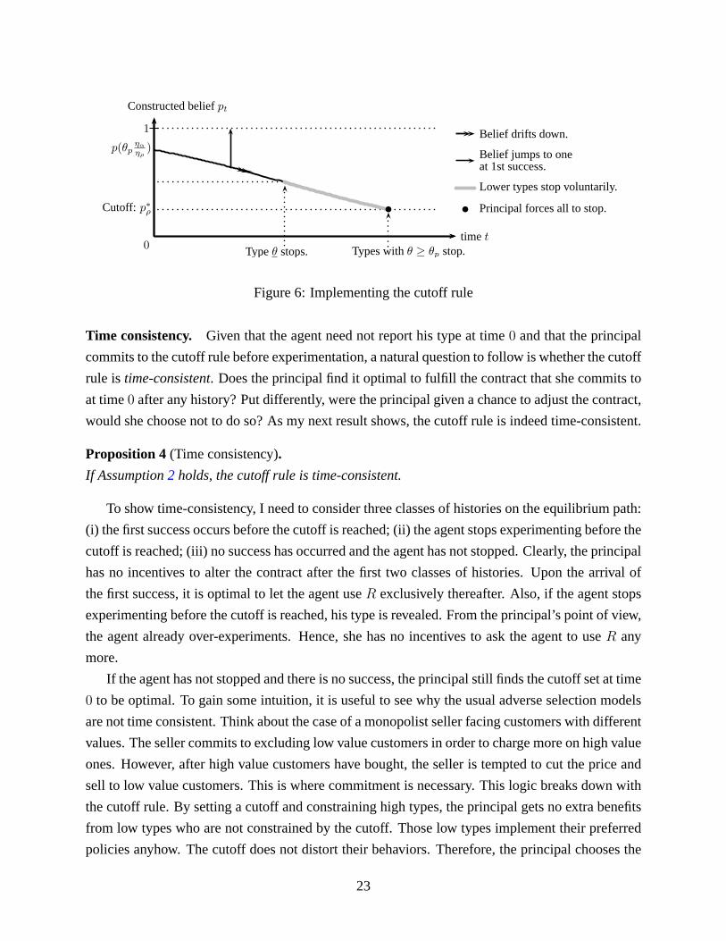
Typeθ stops. Types withθ ≥ θp stop.

b

Belief drifts down.

Belief jumps to oneat 1st success.

Lower types stop voluntarily.

b Principal forces all to stop.

Constructed beliefpt

time t

p(θpηα

ηρ)

Cutoff: p∗ρ

1

0

Figure 6: Implementing the cutoff rule

Time consistency. Given that the agent need not report his type at time0 and that the principal

commits to the cutoff rule before experimentation, a natural question to follow is whether the cutoff

rule is time-consistent. Does the principal find it optimal to fulfill the contract that she commits to

at time0 after any history? Put differently, were the principal given a chance to adjust the contract,

would she choose not to do so? As my next result shows, the cutoff rule is indeed time-consistent.

Proposition 4 (Time consistency).

If Assumption2 holds, the cutoff rule is time-consistent.

To show time-consistency, I need to consider three classes of histories on the equilibrium path:

(i) the first success occurs before the cutoff is reached; (ii) the agent stops experimenting before the

cutoff is reached; (iii) no success has occurred and the agent has not stopped. Clearly, the principal

has no incentives to alter the contract after the first two classes of histories. Upon the arrival of

the first success, it is optimal to let the agent useR exclusively thereafter. Also, if the agent stops

experimenting before the cutoff is reached, his type is revealed. From the principal’s point of view,

the agent already over-experiments. Hence, she has no incentives to ask the agent to useR any

more.

If the agent has not stopped and there is no success, the principal still finds the cutoff set at time

0 to be optimal. To gain some intuition, it is useful to see why the usual adverse selection models

are not time consistent. Think about the case of a monopolistseller facing customers with different

values. The seller commits to excluding low value customersin order to charge more on high value

ones. However, after high value customers have bought, the seller is tempted to cut the price and

sell to low value customers. This is where commitment is necessary. This logic breaks down with

the cutoff rule. By setting a cutoff and constraining high types, the principal gets no extra benefits

from low types who are not constrained by the cutoff. Those low types implement their preferred

policies anyhow. The cutoff does not distort their behaviors. Therefore, the principal chooses the

23

cutoff by looking at only those high types that will be constrained by the cutoff. The cutoffθpis chosen such that conditional on the agent’s type being above θp, the principal finds it optimal

to stop experimenting when the cutoff becomes binding. Thisis why commitment is not required

along the path.

Here, I sketch the proof. First, I calculate the principal’supdated belief about the type distribu-

tion given no success and that the agent has not stopped. By continuing experimenting, the agent

signals that his type is above some level. Hence, the updatedtype distribution is a truncated one.

Since the agent has also updated his belief about the state, Ithen rewrite the type distribution in

terms of the agent’s updated odds ratio. Next I show that given the new type distribution the opti-

mal contract is to continue the cutoff rule set at time0. The detailed proof is relegated to Appendix

8.4.

Over- and under-experimentation. The result of Proposition3 can also be represented by a

delegation rule mapping types into stopping times as only stopping-time policies are assigned in

equilibrium. Figure7 depicts such a rule. Thex-axis variable isθ, ranging fromθ to θ. The dotted

line represents the agent’s preferred stopping time and thedashed line represents the principal’s.16

The delegation rule consists of (i) segment[θ, θp] where the stopping time equals the agent’s pre-

ferred stopping time and (ii) segment[θp, θ] where the stopping time is independent of the agent’s

report (i.e.,pooling segment). To implement, the principal simply imposes a deadline atτα(θp).

Those types withθ ≥ θp all stop atτα(θp), which is the agent’s preferred stopping time given

type θp. Since the principal’s stopping time given typeθpηα/ηρ equals the agent’s stopping time

given θp, the delegation rule intersects the principal’s stopping time at typeθpηα/ηρ. From the

principal’s point of view, those types withθ < θpηα/ηρ experiment too long while those types with

θ > θpηα/ηρ stop too early.

5.4.2 Proof of Proposition3: the optimality of the cutoff rule

To prove Proposition3, I utilize Lagrangian optimization methods (similar to those used by Amador,

Werning, and Angeletos (2006) [4]). It suffices to show that(w1θp, w0

θp) maximizes some La-

grangian functional. Then I establish the sufficient first-order conditions and prove that they are

satisfied at the conjectured contract and Lagrange multipliers.

16Parameters in Figure7 are ηα = 6/5, ηρ = 1, r/λ1 = 1, θ = 1, θ = 5. The type variableθ is uniformlydistributed.

24

Stopping timeτ

typeθ

τα(θp)

Principal’s preferredstopping time

Agent’s preferredstopping time

Delegation rule

θp θpηα

ηρ

Over-experimentation Under-experimentation

θ θ

Figure 7: Equilibrium stopping times

I first extendβse to the real line in the following way:

β(w1) =

(βse)′(0)w1 if w1 ∈ (−∞, 0),

βse(w1) if w1 ∈ [0, w1],

βse(w1) + (βse)′(w1)(w1 − w1) if w1 ∈ (w1,∞).

for some valuew1 such thatw1 ∈ (w1α(θ), 1).

17 The newly defined functionβ is continuously

differentiable, convex and lower thanβse on [0, 1].

I then define a new problemP which differs fromP in two aspects: (i) the upper bound

constraint (10) is dropped; and (ii) the lower bound constraint (9) is replaced with the following:

θηαw1(θ)− ηα

∫ θ

θ

w1(θ)dθ − θηαw1(θ) + w0 − β(w1(θ)) ≥ 0, ∀θ ∈ Θ. (13)

If (w1, w0) satisfies the feasibility constraint (9) and (10), it also satisfies (13). Therefore, the

newly defined problemP is a relaxation ofP. If the solution toP is admissible, I claim that it is

also the solution toP.

Define the Lagrangian functional associated withP as

L(w1, w0 | Λ) = θηαw1(θ)− w0 + ηα

∫ θ

θ

w1(θ)G(θ)dθ

+

∫ θ

θ

(

θηαw1(θ)− ηα

∫ θ

θ

w1(θ)dθ − θηαw1(θ) + w0 − β(w1(θ))

)

dΛ,

17Such aw1 exists becauseθ is finite and hencew1α(θ) is bounded away from1.

25

where the functionΛ is the Lagrange multiplier associated with (13). Fixing a nondecreasing

multiplier Λ, the Lagrangian is a concave functional onΦ because all terms inL(w1, w0 | Λ) are

linear in(w1, w0) except∫ θ

θ−β(w1(θ))dΛ which is concave inw1. Without loss of generality I set

Λ(θ) = 1. Integrating the Lagrangian by parts yields

L(w1, w0 | Λ) =(

θηαw1(θ)− w0

)

Λ(θ) +

∫ θ

θ

(

θηαw1(θ)− β(w1(θ))

)

dΛ (14)

+ ηα

∫ θ

θ

w1(θ) [Λ(θ)− (1−G(θ))] dθ.

The following lemma provides a sufficient condition for a contract(w1, w0) ∈ Φ to solveP.

Lemma 4 (Lagrangian—sufficiency).

A contract(w1, w0) ∈ Φ solvesP if (13) holds with equality and there exists a nondecreasingΛ

such that

L(w1, w0|Λ) ≥ L(w1, w0|Λ), ∀(w1, w0) ∈ Φ.

Proof. I first introduce the problem studied in section 8.4 of Luenberger (1969, p. 220) [21]:

maxx∈X Q(x) subject tox ∈ Ω and J(x) ∈ P , whereΩ is a subset of the vector spaceX,

Q : Ω → R andJ : Ω → Z; whereZ is a normed vector space, andP is a nonempty positive

cone inZ. To apply Theorem1 in Luenberger (1969, p. 220) [21], set

X = w1, w0 | w1 : Θ → R andw0 ∈ R, (15)

Ω = Φ, (16)

Z = z | z : Θ → R with supθ∈Θ

|z(θ)|<∞,

with the norm‖z‖= supθ∈Θ

|z(θ)|,

P = z | z ∈ Z andz(θ) ≥ 0, ∀θ ∈ Θ.

I let the objective function in (OBJ) beQ and let the left-hand side of (13) be defined asJ . This

result holds because the hypotheses of Theorem1 in Luenberger (1969, p. 220) [21] are met.

To apply Lemma4 and show that a proposed contract(w1, w0) maximizesL(w1, w0|Λ) for

some candidate Lagrangian multiplierΛ, I modify Lemma1 in Luenberger (1969, p. 227) [21]

which concerns the maximization of a concave functional in aconvex cone. Note that setΦ is

not a convex cone, so Lemma1 in Luenberger (1969, p. 227) [21] does not apply directly in the

current setting.

26

Lemma 5 (First-order conditions).

LetL be a concave functional onΩ, a convex subset of a vector spaceX. Takex ∈ Ω. Suppose that

the Gâteaux differentials∂L(x; x) and∂L(x; x− x) exist for anyx ∈ Ω and that∂L(x; x− x) =

L(x; x)− L(x; x).18 A sufficient condition thatx ∈ Ω maximizesL overΩ is that

∂L(x; x) ≤ 0, ∀x ∈ Ω,

∂L(x; x) = 0.

Proof. See Appendix8.5.

Next, I prove Proposition3 based on Lemma4 and Lemma5.

Proof. To apply Lemma5, let X andΩ be the same as in (15) and (16). Fixing a nondecreas-

ing multiplier Λ, the Lagrangian (14) is a concave functional onΦ. By applying LemmaA.1 in

Amador, Werning, and Angeletos (2006) [4], it is easy to verify that∂L(w1θp, w0

θp;w1, w0 | Λ) and

∂L(w1θp, w0

θp; (w1, w0) − (w1

θp, w0

θp) | Λ) exist for any(w1, w0) ∈ Φ.19 The linearity condition is

also satisfied

∂L(w1θp , w

0θp ; (w

1, w0)− (w1θp , w

0θp) | Λ) = ∂L(w1

θp , w0θp ;w

1, w0 | Λ)−∂L(w1θp , w

0θp ;w

1θp , w

0θp | Λ).

So the hypotheses of Lemma5 are met. Also, the Gâteaux differential at(w1θp, w0

θp) is given by

∂L(w1θp , w

0θp ;w

1, w0 | Λ) =(

θηαw1(θ)− w0

)

Λ(θ) + ηα

∫ θ

θp

(θ − θp)w1(θ)dΛ (17)

+ ηα

∫ θ

θ

w1(θ) [Λ(θ)− (1−G(θ))] dθ, ∀(w1, w0) ∈ Φ.

Next, I construct a nondecreasing multiplierΛ, in a similar manner as in Proposition3 in Amador,

Werning, and Angeletos (2006) [4], such that the first-order conditions∂L(w1θp, w0

θp;w1, w0 | Λ) ≤

0 and∂L(w1θp, w0

θp;w1

θp, w0

θp| Λ) = 0 are satisfied for any(w1, w0) ∈ Φ.

Let Λ(θ) = 0, Λ(θ) = 1 − G(θ) for (θ, θp], andΛ(θ) = 1 for θ ∈ (θp, θ]. Given thatθp > θ,

I need to show that jumps atθ and θp are upward. The jump atθ is upward since1 − G(θ)

18Let X be a vector space,Y a normed space andD ⊂ X. Given a transformationT : D → Y , if for x ∈ D andx ∈ X the limit

limǫ→0

T (x+ ǫx)− T (x)

ǫ

exists, then it is called the Gâteaux differential atx with directionx and is denoted∂T (x;x). If the limit exists foreachx ∈ X, T is said to be Gâteaux differentiable atx.

19The observations made by Ambrus and Egorov (2013) [5] do not apply to the results of Amador, Werning andAngeletos (2006) [4] that my proof relies on.

27

is nonnegative. The jump atθp is G(θp), which is nonnegative based on the definition ofθp.

Therefore,Λ is nondecreasing.

Substituting the multiplierΛ into the Gâteaux differential (17) yields

∂L(w1θp , w

0θp ;w

1, w0 | Λ) = ηα

∫ θ

θp

w1(θ)G(θ)dθ

= ηα

∫ θ

θp

(

∫ θ

θ

G(θ)dθ

)

dw1(θ),

where the last equality follows by integrating by parts, which can be done given the monotonicity

of w1 and by the definition ofθp. This Gâteaux differential is zero at(w1θp, w0

θp) and, by the

definition ofθp, it is nonpositive for allw1 nondecreasing. It follows that the first-order conditions

are satisfied for all(w1, w0) ∈ Φ. By Lemma5, (w1θp, w0

θp) maximizesL(w1, w0 | Λ) overΦ. By

Lemma4, (w1θp, w0

θp) solvesP. Because(w1

θp, w0

θp) is admissible, it solvesP.

5.4.3 Discussion of Assumption2

In this subsection, I first discuss the economic content of Assumption2. To do so, I consider a

delegation problem in which only bundles onΓst, the southeast boundary ofΓ, are considered. This

restriction reduces the action space to a one-dimensional line segment and allows me to compare

Assumption2 with the condition identified in Alonso and Matouschek (2008) [2]. Then I discuss

the results if Assumption2 fails.

Recall thatΓst is characterized by the functionβse(w1) = 1 − (1 − w1)r/(r+λ1), ∀w1 ∈ [0, 1].

The functionβse is twice continuously differentiable. The derivative(βse)′(w1) strictly increases in

w1 and approaches infinity asw1 approaches1. I identify an element(w1, βse(w1)) ∈ Γst with the

derivative(βse)′(w1) at that point. The set of possible derivatives is denotedY = [(βse)′(0),∞].

Since there is a one-to-one mapping betweenΓst andY , I let Y be the action space and refer to

y ∈ Y as an action. The principal simply assigns a non-empty subset of Y as the delegation set.

Let n(y) = ((βse)′)−1(y) be the inverse of the mapping fromw1 to the derivative(βse)′(w1).

Playeri’s preferred action givenθ is yi(θ) = ηiθ. Playeri’s payoff given typeθ and actiony is

denoted

Vi(θ, y) = ηiθ

1 + θn(y)− 1

1 + θβse(n(y)).

I first solve the principal’s preferred action if she believes that the agent’s type is belowθ. The

principal choosesy ∈ Y to maximize∫ θ

θVρ(θ, y)f(θ)dθ. The maximum is achieved by choosing

action

ηρ

∫ θ

θθh(θ)dθ

H(θ).

28

Following Alonso and Matouschek (2008) [2], I define thebackward biasfor a given typeθ as

T (θ) ≡ H(θ)

H(θ)

(

ηαθ − ηρ

∫ θ

θθh(θ)dθ

H(θ)

)

.

Here,T (θ) measures the difference between the agent’s preferred action givenθ and the principal’s

preferred action if she believes that the type is belowθ. It is easy to verify thatT (θ) = ηα∫ θ

θ(1−

G(θ))dθ.

Assumption2 is equivalent to requiring that the backward bias is convex whenθ ≤ θp. This is

the condition that Alonso and Matouschek (2008) [2] find for the interval delegation set to be opti-

mal in their setting. Intuitively, when this condition holds, the principal finds it optimal to fill in the

“holes” in the delegate set. I shall emphasize that this isnot a proof of the optimality of the cutoff

rule, because considering only bundles on the southeast boundary might be restrictive. For exam-

ple, I have shown that with two types the optimal contract involves bundles which are not on the

southeast boundary for certain parameter values. With a continuum of types, there exist examples

such that the principal is strictly better off by offering policies other than stopping-time policies.

By using Lagrangian methods, I prove that the cutoff rule is indeed optimal under Assumption2.

In my setting, the principal’s preferred bundle is not more sensitive than the agent’s to the agent’s

private information and Assumption2 ensures that the type distribution is sufficiently smooth so

the principal has no particular interest to screen some types. Hence, the interval delegation set is

optimal.

The discussion so far suggests that Assumption2 is also necessary for the cutoff rule to be

optimal. In the rest of this subsection, I show that noxp-cutoff contract is optimal for anyxp ∈ Θ if

Assumption2 does not hold. Thexp-cutoff contract is defined as(w1(θ), w0(θ)) = (w1α(θ), w

0α(θ))

for θ < xp and(w1(θ), w0(θ)) = (w1α(xp), w

0α(xp)) for θ ≥ xp. Thexp-cutoff contract is denoted

(w1xp , w

0xp).

Define the Lagrangian functional associated withP as

L(w1, w0 | Λse,Λnw) = θηαw1(θ)− w0(θ) + ηα

∫ θ

θ

w1(θ)G(θ)dθ (18)

+

∫ θ

θ

(

θηαw1(θ)− ηα

∫ θ

θ

w1(θ)dθ − θηαw1(θ) + w0 − βse(w1(θ))

)

dΛse

+

∫ θ

θ

[

βnw(w1(θ))−(

θηαw1(θ)− ηα

∫ θ

θ

w1(θ)dθ − θηαw1(θ) + w0

)]

dΛnw,

where the functionΛse,Λnw are the Lagrange multiplier associated with constraints (9) and (10).

I first show that if(w1xp , w

0xp) is optimal for somexp, there must exist some Lagrange multipliers

29

Λse, Λnw such thatL(w1, w0 | Λse, Λnw) is maximized at(w1xp , w

0xp). Since anyxp-cutoff contract

is continuous, I can restrict attention to the set of continuous contracts

Φ ≡

w1, w0 | w1 : Θ → [0, 1], w1 nondecreasing and continuous;w0 ∈ [0, 1]

.

Lemma 6 (Lagrangian—necessity).

If (w1xp , w

0xp) solvesP, then there exist two nondecreasing functionsΛse, Λnw : Θ → R such that

L(w1xp , w

0xp | Λse, Λnw) ≥ L(w1, w0 | Λse, Λnw), ∀(w1, w0) ∈ Φ.

Furthermore, it is the case that

0 =

∫ θ

θ

(

θηαw1xp(θ)− ηα

∫ θ

θ

w1xp(θ)dθ − θηαw

1xp(θ) + w0

xp − βse(w1xp(θ))

)

dΛse (19)

+

∫ θ

θ

[

βnw(w1xp(θ))−

(

θηαw1xp(θ)− ηα

∫ θ

θ

w1xp(θ)dθ − θηαw

1xp(θ) + w0

xp

)]

dΛnw.

Proof. This is a direct application of Theorem1 in Luenberger (1969, p. 217) [21]. The proof is

relegated to Appendix8.6.

My next result shows that noxp-cutoff contract is optimal if Assumption2 fails.

Proposition 5.

If Assumption2 does not hold, then noxp-cutoff contract is optimal for anyxp ∈ Θ.

Proof. The proof proceeds by contradiction. Suppose that(w1xp , w

0xp) is optimal for somexp ∈

Θ. According to Lemma6, there exist nondecreasingΛse, Λnw such that the Lagrangian (18) is

maximized at(w1xp , w

0xp) and (19) holds. This implies thatΛnw is constant so the integral related

to Λnw can be dropped. Without loss of generality I setΛse(θ) = 1. Integrating the Lagrangian by

parts yields

L(w1, w0 | Λse) =(

θηαw1(θ)− w0

)

Λse(θ) +

∫ θ

θ

(

θηαw1(θ)− βse(w1(θ))

)

dΛse

+ ηα

∫ θ

θ

w1(θ)[

Λse(θ)− (1−G(θ))]

dθ.

Then, I establish the necessary first-order conditions forL(w1, w0 | Λse) to be maximized atxp-

cutoff rule and show that they cannot be satisfied if Assumption 2 fails. The rest of the proof is

relegated to Appendix8.7.

30

6 Extensions

6.1 More general stochastic processes

6.1.1 Inconclusive successes

Now suppose thatλ0 > 0, soR generates successes in state0 as well and players never fully

learn the state. In this subsection, unless otherwise specified, I use the same notations as in the

benchmark setting. Recall that(w1(π),w0(π)) denotes theexpected resourceallocated toR under

π conditional on state1 and state0, andΓ the image of the mapping(w1,w0) : Π → [0, 1]2. The

following lemma characterizes the feasible setΓ.

Lemma 7 (Inconclusive news—feasible set).

There exist two functionsβse, βnw : [0, 1] → [0, 1] such thatΓ = (w1, w0) | βse(w1) ≤ w0 ≤βnw(w1), w1 ∈ [0, 1]. The southeast boundary is given byβse(w1) = 1 − (1 − w1)µ/(1+µ), for

some constantµ > 0. The northwest boundaryβnw is concave, nondecreasing, once continuously

differentiable, having end points(0, 0) and(1, 1).

Proof. The proof is similar to that of Lemma3 and relegated to Appendix8.8

Figure 8 depicts the feasible set whenr = 1/5, λ1 = 2/5, λ0 = (2 −√2)/5. Unlike the

benchmark setting, the northwest boundary is characterized by a once continuously differentiable

function. My next result shows that, if Assumption2 holds, the cutoff rule as defined in Definition

1 is optimal. This is the case because the proof of Proposition3, which only relies on the properties

of the southeast boundary of the feasible set, applies directly to the current setting.

Proposition 6 (Inconclusive news—sufficiency).

If Assumption2 holds, the cutoff rule is optimal.

Proof. According to Lemma7, the southeast boundary of the feasible set is given byβse(w1) =

1− (1−w1)µ/(1+µ), for some constantµ > 0. The proof of Proposition3 applies directly here.

The implementation of the cutoff rule, similar to that of thebenchmark setting, is achieved by

calibrating a constructed belief which starts with the prior beliefp(θpηρ/ηα). This belief is updated

as follows: (i) if no success occurs, the belief drifts down according to the differential equation

pt = −(λ1 − λ0)pt(1− pt); and (ii) if a success occurs at timet, the belief jumps frompt− to

pt =λ1pt−

λ1pt− + λ0(1− pt−).

The principal imposes a cutoff atp∗ρ. The agent can choose to experiment or not if this belief stays

above the cutoff and are required to stop when it drops to the cutoff. The gray areas in Figure9

31

w0(π)

w1(π)0 1

1

Feasible set:Γb

θηα

bθηα

bθηρ

b

θηρbθpηα

Delegation set

Agent’s preferredbundles

Principal’s preferredbundles

Figure 8: Delegation set under cutoff rule: inconclusive news case

show that lower types stop voluntarily as their posterior beliefs reachp∗α. The black dot shows that

those types withθ > θp are required to stop.

Figure9 also highlights the difference between the benchmark setting, where the belief jumps

to one after the first success, and the inconclusive news setting, where the belief jumps up upon

successes and then drifts down. Consequently, when successes are inconclusive, the optimum

can no longer be implemented by imposing a fixed deadline. Instead, it takes the form of a sliding

deadline. The principal initially extends some time to the agent. Then, whenever a success realizes,

more time is extended. The agent is allowed to give up his timevoluntarily. That is, the agent can

choose to switch toS before he uses up the time granted by the principal. After a long enough

period of time elapses without success, the principal requires the agent to switch toS.

Typeθ stops. Types withθ ≥ θp stop.

b

Belief drifts down.

Belief jumps at successes.

Lower types stop voluntarily.

b Principal forces all to stop.

Constructed beliefpt

time t

p(θpηα

ηρ)

Cutoff: p∗ρ

1

0

Figure 9: Implementing the cutoff rule: inconclusive news

32

My next result shows that the cutoff rule is time consistent when successes are inconclusive.

The intuition is exactly the same as in the benchmark settingyet the proof is slightly different.

Since successes never fully reveal the state, I need to show that the principal finds it optimal not to

adjust the cutoff upon successes. The detailed proof is relegated to Appendix8.9.

Proposition 7 (Inconclusive news—time consistency).

If Assumption2 holds, the cutoff rule is time-consistent.

Proof. See Appendix8.9.

6.1.2 Lévy processes and Lévy bandits

Here, I extend the analysis to the more general Lévy bandits (Cohen and Solan, 2013 [11]). The

risky task’s payoff is driven by a Lévy process whose Lévy triplet depends on an unknown binary

state. In what follows, I start with a reminder about Lévy processes and Lévy bandits. Then, I

show that the optimality of the cutoff rule and its time consistency property generalize to Lévy

bandits.

Lévy processes. A Lévy processL = (L(t))t≥0 is a continuous-time stochastic process that (i)

starts at the origin:L(0) = 0; (ii) admits càdlàg modification;20 (iii) has stationary independent

increments. Examples of Lévy processes include a Brownian motion, a Poisson process, and a

compound Poisson process.

Let (Ω, P ) be the underlying probability space. For every Borel measurable setA ∈ B(R\0),and everyt ≥ 0, let the Poisson random measureN(t, A) be the number of jumps ofL in the time

interval [0, t] with jump size inA: N(t, A) = #0 ≤ s ≤ t | ∆L(s) ≡ L(s)− L(s−) ∈ A. The

measureν defined by

ν(A) ≡ E[N(1, A)] =

∫

N(1, A)(ω)dP (ω).

is called theLévy measureof the processL.

I focus on Lévy processes that have finite expectation for each t. For a fixed Lévy processL,

there exists a constantµ ∈ R, a Brownian motionσZ(t) with standard deviationσ ≥ 0, and an

independent Poisson random measureNν(t, dh) with the associated Lévy measureν such that, for

eacht ≥ 0, the Lévy-Ito decomposition ofL(t) is

L(t) = µt+ σZ(t) +

∫

R\0

hNν(t, dh),

20It is continuous from the right and has limits from the left.

33

whereNν(t, A) ≡ Nν(t, A) − tν(A) is the compensated Poisson random measure.21 Hence, a

Lévy processL is characterized by a triplet〈µ, σ, ν〉.

Lévy bandits. The agent operates a two-armed bandit in continuous time, with a safe armS

that yields a known flow payoffsi to playeri, and a risky armR whose payoff, depending on an

unknown statex ∈ 0, 1, is given by the processLx. For ease of exposition, I assume that both

players derive the same payoff fromR but different payoffs fromS. For a fixed statex, Lx is a

Lévy process characterized by the triplet〈µx, σx, νx〉. For an arbitrary priorp that the state is1, I

denote byPp the probability measure over space of realized paths.

I keep the same assumptions (A1–A6) on the Lévy processesLx as in Cohen and Solan (2013)

[11] and modify A5 to ensure that both players prefer to useR in state1 andS in state0. That is,

µ1 > si > µ0, for i ∈ α, ρ.22 Let ηi = (µ1 − si)/(si − µ0) denote playeri’s net gain from the

experiment. I assume that the agent gains more from the experiment,i.e., ηα > ηρ. 23

Policies and feasible set. A (pure) allocation policy is a non-anticipative stochastic processπ =

πtt≥0. Here,πt ∈ [0, 1] (resp.1 − πt) may be interpreted as the fraction of time in the interval

[t, t+ dt) that is devoted toR (resp.S), which may depend only on the history of events up tot.24

The space of all policies, including randomized ones, is denotedΠ. (See Footnote8.)

Playeri’s payoff given a policyπ ∈ Π and a prior beliefp ∈ [0, 1] that the state is1 is

Ui(π, p) ≡ E

[∫ ∞

0

re−rt[

dLx(∫ t

0

πsds

)

+ (1− πt) sidt

]

∣

∣

∣π, p

]

.

Over an interval[t, t+dt), if the fractionπt of time is allocated toR, the expected payoff increment

to playeri conditional onx is [(1 − πt)si + πtµx]dt. By the Law of Iterated Expectations, I can

21Consider a setA ∈ B(R \ 0) and a functionf : R → R. The integral with respect to a Poisson randommeasureN(t, A) is defined as

∫

Af(h)N(t,dh) =

∑

s≤t f(∆L(s))1A(∆(L(s))).22The assumptions are (A1)E[(Lx)2(1)] = (µx)2+(σx)2+

∫

h2νx(dh) < ∞; (A2) σ1 = σ0; (A3) |ν1(R\0)−ν0(R \ 0)|< ∞; (A4) |

∫

h(ν1(dh) − ν0(dh))|< ∞; (A5) µ0 < sα < sρ < µ1; (A6) For everyA ∈ B(R \ 0),ν0(A) < ν1(A). Assumption (A1) states that bothL1 andL0 have finite quadratic variation. It follows that bothhave finite expectation. Assumptions (A2) to (A4) ensure that players cannot distinguish between the two states inany infinitesimal time. Assumption (A5) states that the expected payoff rate ofR is higher than that ofS in state1and lower in state0. The last assumption (A6) requires that jumps of any sizeh, both positive or negative, occur moreoften in state1 than in state0. Consequently, jumps always provide good news, and increase the posterior belief ofstate1.

23The results generalize to the case in which, for a fixed statex, the drift term of the Lévy processLx differs for theprincipal and the agent, as long as the relationηα > ηρ holds.

24Suppose the processL is a Lévy processL1 with probability p ∈ (0, 1) andL0 with probability 1 − p. LetFL

s be the sigma-algebra generated by the process(L(t))t≤s. Then it is required that the processπ satisfies that∫ t

0πsds ≤ t′ ∈ FL

t′ , for anyt, t′ ∈ [0,∞).

34

write playeri’s payoff as the discounted sum of the expected payoff increments

Ui(π, p) = E

[∫ ∞

0

re−rt [πtµx + (1− πt)si] dt

∣

∣

∣π, p

]

.

For a fixed policyπ, I definew1(π) andw0(π) as follows:

w1(π) ≡ E

[∫ ∞

0

re−rtπtdt∣

∣

∣π, 1

]

andw0(π) ≡ E

[∫ ∞

0

re−rtπtdt∣

∣

∣π, 0

]

.

Then, playeri’s payoff can be written as

Ui(π, p) = p(

µ1 − si)

w1(π) + (1− p)

(

µ0 − si)

w0(π) + si.

Let Γ denote the image of the mapping(w1,w0) : Π → [0, 1]2, referred to as the feasible set. The

following lemma characterizes the southeast boundary ofΓ.

Lemma 8. There existsa∗ > 0 such that the southeast boundary ofΓ is given by

(w1, w0) | w0 = 1− (1− w1)a∗/(1+a∗), w1 ∈ [0, 1]

Proof. The proof is similar to that of Lemma3 and relegated to Appendix8.10

Given Lemma8, the proof of Proposition3, which only relies on the properties of the southeast

boundary of the feasible set, applies directly to the current setting. Therefore, the cutoff rule as

defined in Definition1 is optimal under Assumption2.

Proposition 8 (Lévy bandits—sufficiency).

The cutoff rule is optimal if Assumption2 holds.

For every priorp ∈ [0, 1] that the state is1, the probability measurePp satisfiesPp = pP1 +

(1− p)P0. An important auxiliary process is the Radon-Nikodym density, given by

ψt ≡d(P0 | FK(t))

d(P1 | FK(t)), whereK(t) =

∫ t

0

πsds andt ∈ [0,∞).

According to Lemma1 in Cohen and Solan (2013) [11], if the prior belief isp, the posterior belief

at timet is given by

pt =p

p+ (1− p)ψt.

The agent of typeθ updates his belief about the state. He assigns odds ratioθ/ψt to the state being

1, referred to as his type at timet. Let θt = maxθ, θ∗αψt. Recall thatθ∗α denotes the odds ratio at

35

which the agent is indifferent between continuing and stopping. At time t, only those types above

θt remain. The principal’s updated belief about the agent’s type distribution,in terms of his type at

time0, is given by the density function

f(θ | t) =

[p(θ)+(1−p(θ))ψt]f(θ)∫ θθt[p(θ)+(1−p(θ))ψt]f(θ)dθ

if θ ∈ [θt, θ],

0 otherwise.

The principal’s belief about the agent’s type distribution, in terms of his type at timet, is given by

the density function

ft(θ) =

f(θψt | t)ψt if θ ∈ [θt/ψt, θ/ψt],

0 otherwise.

I prove that continuing the cutoff rule is optimal by showingtwo things. First, given the distribution

ft at timet, the threshold of the top pooling segment isθp/ψt. Second, if Assumption2 holds for

θ ≤ θp under distributionf , then it holds forθ ≤ θp/ψt underft. The detailed proof is similar to

that of Proposition7 (see Appendix8.4) and hence omitted.

Proposition 9 (Lévy bandits—time consistency).

If Assumption2 holds, the cutoff rule is time-consistent.

6.2 Biased toward the safe task: a lockup period

In this subsection, I consider the situations in which the agent is biased toward the safe task,i.e.,

ηα < ηρ. This happens, for example, when a division (agent) conducts an experiment which yields

positive externalities to other divisions. Hence, the agent does not internalize the total benefit that

the experiment brings to the organization (principal). Another possibility is that the agent does

not perceive the risky task to generate significant career opportunities compared with alternative

activities. In both cases, the agent has a preference to stopexperimenting earlier.

To illustrate the main intuition, I assume that the lowest type agent prefers a positive length

of experimentation,i.e., τα(θ) > 0. Using the same methods as in the main model, I first show

that types below some threshold are pooled. Intuitively, types at the bottom prefer to experiment

less than what the principal prefers to do for any prior. The cost of separating those types exceeds

the benefit. Then, I show that under certain condition the optimal outcome for the principal can

be implemented by starting with a properly calibrated priorbelief that the state is1. This belief

is then updated as if the agent had no private information. Aslong as this belief remains above

a cutoff belief, the agent is required to operateR. As soon as it drops to the cutoff, the principal

keeps her hands off the project and lets the agent decide whether to experiment or not.

36

Notably, in contrast to the main model, the agent has no flexibility until the cutoff belief is

reached. I call this mechanism thereversed cutoff rule. Those types with low enough priors stop

experimenting as soon as the cutoff is reached. Those with higher priors are not constrained and

thus implement their preferred policies.

If successes are conclusive, the principal simply sets up alockup periodduring which the agent

usesR regardless of the outcome. After the lockup period ends, theagent is free to experiment

or not. If successes are inconclusive, the principal initially sets up a lockup length. Each time a

success occurs, the lockup length is extended. The agent hasno freedom until the lockup period

ends.

Given a direct mechanism(w1(θ), w0(θ)), letUα(θ) denote the payoff that the agent of typeθ

gets by maximizing over his report. As the optimal mechanismis truthful,Uα(θ) equalsθηαw1(θ)−w0(θ) and the envelope condition implies thatU ′

α(θ) = ηαw1(θ). By integrating the envelope

condition, one obtains the standard integral condition

θηαw1(θ)− w0(θ) = θηαw

1(θ)− w0 −∫ θ

θ

ηαw1(θ)dθ,

wherew0 stands forw0(θ). Substitutingw0(θ) and simplifying, I reduce the problem to finding a

functionw1 : Θ → [0, 1] and a scalarw0 that solves

maxw1,w0∈Φs

(

θηαw1(θ)− w0 − ηα

∫ θ

θ

w1(θ)Gs(θ)dθ

)

, (OBJ-S)

subject to

θηαw1(θ) +

∫ θ

θ

ηαw1(θ)dθ − θηαw

1(θ) + w0 − βse(w1(θ)) ≥ 0, ∀θ ∈ Θ, (20)

βnw(w1(θ))−(

θηαw1(θ) +

∫ θ

θ

ηαw1(θ)dθ − θηαw

1(θ) + w0

)

≥ 0, ∀θ ∈ Θ, (21)

where

Φs ≡

w1, w0 | w1 : Θ → [0, 1], w1 nondecreasing;w0 ∈ [0, 1]

,

Gs(θ) =H(θ)

H(θ)+

(

1− ηρηα

)

θh(θ)

H(θ), whereh(θ) =

f(θ)

1 + θandH(θ) =

∫ θ

θ

h(θ)dθ.

37

I denote this problem byPs. Let θsp be the highest value inΘ such that

∫ θ

θ

Gs(θ)dθ ≤ 0, for any θ ≤ θsp. (22)

My next result shows that types withθ ≤ θsp are pooled.

Proposition 10(Pooling on bottom).

An optimal contract(w1∗, w0∗) satisfiesw1∗(θ) = w1∗(θsp) for θ ≤ θsp. It is optimal for(20) or (21)

to hold with equality atθsp.

Proof. The contribution to (OBJ-S) from types withθ < θsp is−ηα∫ θspθw1(θ)Gs(θ)dθ. Substituting

w1(θ) = w1(θsp)−∫ θspθ

dw1 and integrating by parts, I obtain

− ηα

∫ θsp

θ

w1(θ)Gs(θ)dθ = −ηαw1(θsp)

∫ θsp

θ

Gs(θ)dθ + ηα

∫ θsp

θ

∫ θ

θ

Gs(θ)dθdw1(θ). (23)

The first term only depends onw1(θsp). The second term depends ondw1(θ) for all θ ∈ [θ, θsp].

According to the definition ofθsp, the integrand of the second term,∫ θ

θGs(θ)dθ, is weakly negative

for all θ ∈ [θ, θsp]. Therefore, it is optimal to setdw1(θ) = 0 for all θ ∈ [θ, θsp]. If θsp = θ, all

types are pooled. The principal offers her preferred uninformed bundle, which is on the southeast

boundary ofΓ. If θsp < θ, the first term of (23) is zero as well because∫ θspθGs(θ)dθ = 0. Adjusting

w1(θsp) does not affect the objective function, sow1(θsp) can be decreased until either (20) or (21)

binds.

For the rest of this subsection, I focus on the more interesting case in whichθsp < θ. I first

define the reversed cutoff rule.

Definition 2. Thereversed cutoff ruleis the contract(w1, w0) such that

(w1(θ), w0(θ)) =

(w1α(θ

sp), w

0α(θ

sp)) if θ ≤ θsp,

(w1α(θ), w

0α(θ)) if θ > θsp.

I denote this rule by(w1θsp, w0

θsp). My next result gives a sufficient condition under which the

reserved cutoff rule is optimal.

Proposition 11(Sufficiency-reversed cutoff rule).

The reversed cutoff rule(w1θsp, w0

θsp) is optimal ifGs(θ) is nondecreasing whenθ ≥ θsp.

If f(θ) is differentiable,Gs(θ) being nondecreasing forθ ≥ θsp is equivalent to requiring that

θf ′(θ)

f(θ)≤ ηαηρ − ηα

− 1

1 + θ, ∀θ ∈ [θsp, θ].

38

It is satisfied for any densityf with θf ′/f bounded from above whenηρ/ηα is sufficiently close to

1, or equivalently when two players’ preferences are sufficiently aligned.

Proof. I define a new problemPs which differs fromPs in two aspects: (i) the upper bound

constraint (21) is dropped; and (ii) the lower bound constraint (20) is replaced with the following:

θηαw1(θ) +

∫ θ

θ

ηαw1(θ)dθ − θηαw

1(θ) + w0 − β(w1(θ)) ≥ 0, ∀θ ∈ Θ.

Define the Lagrangian functional associated withPs as

Ls(w1, w0 | Λ) = θηαw1(θ)− w0 − ηα

∫ θ

θ

w1(θ)Gs(θ)dθ

+

∫ θ

θ

(

θηαw1(θ) +

∫ θ

θ

ηαw1(θ)dθ − θηαw

1(θ) + w0 − β(w1(θ))

)

dΛ.

Integrating by parts and simplifying, I obtain

Ls(w1, w0 | Λ) =(

θηαw1(θ)− w0

)

(1− Λ(θ) + Λ(θ)) +

∫ θ

θ

(

θηαw1(θ)− β(w1(θ))

)

dΛ

+ ηα

∫ θ

θ

(Λ(θ)− Λ(θ)−Gs(θ))w1(θ)dθ

Based on Lemma4 and Lemma5, it suffices to show that the following first-order conditions hold

for some candidate multiplierΛ,

Ls(w1θsp, w0

θsp;w1, w0 | Λ) ≤ 0, ∀(w1, w0) ∈ Φs

Ls(w1θsp, w0

θsp;w1

θsp, w0

θsp| Λ) = 0.

If Gs(θ) is nondecreasing whenθ ∈ [θp, θ], the first-order conditions are satisfied given the follow-

ing candidate multiplier

Λ(θ) =

0 if θ ∈ [θ, θsp),

Gs(θ) if θ ∈ [θsp, θ),

1 if θ = θ.

The jump atθsp is nonnegative according to the definition ofθsp. The jump atθ is nonnegative

becauseGs(θ) ≤ 1 for all θ. This completes the proof.

39

6.3 Heterogeneous beliefs

The analysis can be extended to the situation in which beliefs are heterogeneous. Suppose that

the two players differ in their prior beliefs about the state. At time 0, the agent obtains a private

informative signal about the state. Due to difference in their prior beliefs, the principal’s belief

about the state distribution would differ from that of the agent even if she observed the agent’s

signal. To illustrate, suppose that there is no fundamentalpreference conflict. The results in the

benchmark setting are applicable in the situation where theagent is more optimistic and assigns

a higher odds ratio to state1 than the principal for any fixed signal. The agent has an incentive

to misrepresent his information to counteract the principal’s pessimism (from the agent’s point of

view). There are many other possible forms of different opinions. For example, the agent might

be more pessimistic or disagree with the principal about theinformativeness of his private signal.

The analysis can be easily modified to incorporate those situations.

6.4 Social planner’s problem

Here, I consider a social planner who seeks to maximize the weighted sum of the two players’

payoffs. The social planner determines a delegation set at time 0, knowing that the agent chooses

a bundle to maximize his own payoff. The social planner’s gain from R’s successes relative to

S’s flow payoffs can be summarized by a constant, denotedηs, which is a weighted average ofηρandηα. As a result, the social planner’s problem is similar to the principal’s problem, the only

difference being that the bias term is smaller since the agent’s welfare is taken into account. In

general, the social planner prefers to give the agent more flexibility than the principal does.

If assumption2 holds forθ ∈ Θ, the optimal solution to the social planner’s problem is also

a cutoff rule. Moreover, based on Corollary2, the threshold of the pooling segmentθp is an

increasing function of the weight put on the agent’s welfare. Therefore, the more weight is put on

the agent’s welfare, the more flexibility shall be granted tothe agent.

7 Concluding remarks

This paper discusses how organizations can optimally manage innovative activities, particularly

how much control right over resource allocation shall be left to the agent over time with the pres-

ence of misaligned preferences and hidden information. From this aspect, this paper contributes to

the discussion of how to optimally allocate formal authority and real authority within organizations

(Aghion and Tirole, 1997 [1]).

The optimal delegation rule requires the agent to achieve a success before the next deadline to

keep the project alive. It is simple, time-consistent and already implemented in organizations such

40

as Google. Google encourages its employees to come up with new ideas and build a prototype. If

the initial result is satisfactory, Google makes it an official project, funds it and sets the next pair of

goal and deadline. The goal must be met before the deadline tosecure future funding. Successful

products including Gmail, Google Earth and Google Maps survived all the deadlines. Needless to

say, many more did not. For example, the once highly publicized and well-funded Google Wave

was canceled in August2010 as it failed to achieve the goal set by Google executives before then.

Besides in-house innovation, my results also apply to the government sector, which often ex-

periments reforms in public policy. The constituents delegate reforms to politicians. Legislatures

delegate policy-making to their standing committees. Throughout the process transfers are prohib-

ited to prevent corruption. It has been concluded that everyreform has consequences that cannot

be fully known until it has been implemented (Strulovici, 2010 [24]). The constituents as well as

the government learn the effects of a reform that gradually unfold. If a reform is thought to be a

failure, it can be legislatively repealed, executively overturned or allowed to automatically expire

with a sunset provision. Politicians hope to prolong the policy experimentation as they gain the

most popularity from successful reforms that they initiated. My sliding deadline rule suggests that

if politicians are better informed on policies, every reform should carry a sunset provision. They

should be renewed only upon demonstrated successes.

41

8 Appendix

8.1 Proof of Proposition1

Let αl (resp.αh) denote the low (resp. high) type agent andρl (resp.ρh) the low (resp. high) type

principal.

1. Suppose thatθlηρ > r/(λ1 + r). Bothρl’s andρh’s preferred bundles lie in the interior ofΓst.

Given thatθh > θl andηα > ηρ, the slopes of players’ indifference curves are ranked as follows

θhηα > maxθhηρ, θlηα ≥ minθhηρ, θlηα > θlηρ.

Let ICL and ICH denoteαl’s andαh’s IC constraints. LetIαldenoteαl’s indifference curves.

If αl prefers(w1ρ(θl), w

0ρ(θl)) to (w1

ρ(θh), w0ρ(θh)), the optimum is

(w1ρ(θl), w

0ρ(θl)), (w

1ρ(θh), w

0ρ(θh)).

This is the case when the slope of the line connecting(w1ρ(θl), w

0ρ(θl)) and(w1

ρ(θh), w0ρ(θh)) is

greater thanθlηα. This condition is satisfied whenηα/ηρ is bounded from above by

b′ ≡θh(λ

1 + r)(

θhr

λ1 − θlr

λ1

)

r(

θhr+λ1

λ1 − θlr+λ1

λ1

) .

If this condition does not hold, at least one IC constraint binds. I explain how to find the optimal

bundles.

Step 1. ICL binds. Suppose not. It must be the case that ICH binds. Given that ICL does

not bind and ICH binds, the principal offers two distinct bundles (w1(θl), w0(θl)) <

(w1(θh), w0(θh)) which lie on the same indifference curve ofαh. Given thatθhηα >

maxθhηρ, θlηρ, both ρh andρl strictly prefer(w1(θl), w0(θl)) to (w1(θh), w

0(θh)).

The principal is strictly better off by offering a pooling bundle (w1(θl), w0(θl)). Con-

tradiction. Hence, ICL holds with equality.

Step 2. If θhηρ < θlηα, the optimum is pooling.Suppose not. Suppose that the principal offers

two distinct bundles(w1(θl), w0(θl)) < (w1(θh), w

0(θh)) which are on the same indif-

ference curve ofαl. Given thatθlηρ < θhηρ < θlηα, αl’s indifference curves are steeper

thanρh’s andρl’s. Both ρh andρl strictly prefer(w1(θl), w0(θl)) to (w1(θh), w

0(θh)).

The principal is strictly better off by offering a pooling bundle (w1(θl), w0(θl)). Con-

tradiction.

42

b

(w1(θl), w0(θl))

b

(w1(θh), w0(θh))

Iαl

b

(w1(θl), w0(θl))

b(w1(θh), w

0(θh))w

0(π)

w1(π)0 1

1

Figure 10:Optimum bundles are on the boundary

IαlIαl

Iαl

b

(w1α(θl), w

0α(θl))

b(w1

ρ(θl), w0ρ(θl))

b(w1

ρ(θh), w0ρ(θh))

b

C

w0(π)

w1(π)0 1

1

Figure 11:Location of optimal bundles

Step 3. If θhηρ > θlηα, the optimal bundles are on the boundary ofΓ. Suppose not. Sup-

pose that(w1(θl), w0(θl)) or (w1(θh), w

0(θh)) is in the interior. The indifference curve

of αl going through(w1(θl), w0(θl)) intersects the boundary at(w1(θl), w

0(θl)) and

(w1(θh), w0(θh)). Given thatθhηρ > θlηα > θlηρ, ρh prefers(w1(θh), w

0(θh)) to

(w1(θh), w0(θh)) andρl prefers(w1(θl), w

0(θl)) to (w1(θl), w0(θl)). The principal is

strictly better off by offering(w1(θl), w0(θl)) and (w1(θh), w

0(θh)) (see Figure10).

Therefore, the optimal bundles are on the boundary. The problem is reduced to locate

the low type agent’s indifference curve on which(w1∗(θl), w0∗(θl)) and(w1∗(θh), w

0∗(θh))

lie. I want to show that this indifference curve must be between the indifference curves

of αl which go through(w1ρ(θl), w

0ρ(θl)) and(w1

ρ(θh), w0ρ(θh)) (see Figure11). Suppose

not. Suppose the optimal bundles are pinned down by the dashed indifference curve of

αl as shown in Figure11. The principal is strictly better off by offering(w1ρ(θl), w

0ρ(θl))

andC. Analogously, the optimal bundles cannot lie on the indifference curve which lies

to the southeast of the indifference curve that goes through(w1ρ(θh), w

0ρ(θh)).

Step 4. If θhηρ = θlηα, there exists an optimal pooling bundle.If the principal finds it optimal

to offer two distinct contracts(w1(θl), w0(θl)), (w

1(θh), w0(θh)), it must be the case

that (w1(θl), w0(θl)) and (w1(θh), w

0(θh)) are on the same indifference curve ofαl.

Sinceαl’s indifference curve is steeper thanρl’s, (w1(θl), w0(θl)) lies on the boundary

of Γ and(w1(θh), w0(θh)) is located to the northeast of(w1(θl), w

0(θl)). Sinceρh has

the same indifference curves asαl, it is optimal for the principal to offer a pooling

contract(w1(θl), w0(θl)) if (w1(θl), w

0(θl)), (w1(θh), w

0(θh)) is optimal.

43

Combining Step 2 and 4, I obtain that pooling is optimal whenηα/ηρ ≥ θh/θl. This completes

the proof of Proposition1.

2. Suppose thatθhηρ ≤ r/(r + λ1). Both ρh andρl prefer to stop at time0. The optimum is

(w1∗(θl), w0∗(θl)) = (w1∗(θh), w

0∗(θh)) = (0, 0).

3. Suppose thatθlηρ ≤ r/(r + λ1) < θhηρ, the principal optimally offers her preferred bundles if

θlηα ≤1−

(

ηρθh(λ1+r)

r

)− r

λ1

1−(

ηρθh(λ1+r)

r

)−λ1+r

λ1

.

If this does not hold andθlηα < θhηρ , the principal offers two bundles on the same indifference

curve of the low type agent. Both bundles are on the boundary ofΓ. If θlηα ≥ θhηρ, pooling is

optimal. The proof is similar as in case1.

8.2 Proof of Corollary 1

SubstitutingG(θ) = 1H(θ)

(

∫ θ

θh(θ)dθ +

(

ηρηα

− 1)

θh(θ))

and integrating by parts, I obtain

∫ θ

θ

G(θ)dθ =1

H(θ)

∫ θ

θ

[

∫ θ

θ

h(θ)dθ +

(

ηρηα

− 1

)

θh(θ)

]

dθ

=1

H(θ)

∫ θ

θ

[

(θ − θ)h(θ) +

(

ηρηα

− 1

)

θh(θ)

]

dθ

=1

H(θ)

∫ θ

θ

(

ηρηαθ − θ

)

h(θ)dθ.

For anyθ ∈ [θηρ/ηα, θ], the integrand(θηρ/ηα − θ)h(θ) is weakly negative for anyθ ∈ Θ. There-

fore, θp ≤ θηρ/ηα. If θp > θ, θp is strictly belowθηρ/ηα. Otherwise,h(θ) must equal0 for

θ ∈ [θηρ/ηα, θ]. Contradiction.25

8.3 Proof of Corollary 2

LetG(θ, z) be the value ofG(θ) if ηρ/ηα equalsz ∈ [0, 1], i.e.,

G(θ, z) =H(θ)−H(θ)

H(θ)+ (z − 1)θ

h(θ)

H(θ).

25If θp > θ, I obtain that∫ θ

θp(ηρθ − ηαθp)h(θ)dθ = 0.

44

Let θp(z) be the lowest value inΘ such that∫ θ

θG(θ, z)dθ ≤ 0 for any θ ≥ θp(z). BecauseG(θ, z)

is an increasing function ofz for a fixedθ ∈ Θ, θp(z) also increases inz.

If z = 1,G(θ, 1) = (H(θ)−H(θ))/H(θ). Supposeθp(1) < θ. Given the definition ofθp(1), I

have

∫ θ

θp(1)

G(θ, 1)dθ =1

H(θ)

∫ θ

θp(1)

(H(θ)−H(θ))dθ

=1

H(θ)

∫ θ

θp(1)

(θ − θp(1))h(θ)dθ ≤ 0.

This implies thath(θ) = 0 for all θ ∈ [θp(1), θ]. Contradiction. Therefore,θp(1) = θ.

For anyθ ∈ Θ andz ∈ [0, 1], I have

∫ θ

θ

G(θ, z)dθ =1

H(θ)

(

∫ θ

θ

(z − 1)θh(θ)dθ +∫ θ

θ

(θ − θ)h(θ)dθ

)

=1

H(θ)

(

z

∫ θ

θ

θh(θ)dθ − θ

∫ θ

θ

h(θ)dθ

)

.

Let z∗ beminθ∈Θ

(

θ∫ θ

θh(θ)dθ

)

/(

∫ θ

θθh(θ)dθ

)

. If z ≤ z∗,∫ θ

θG(θ, z)dθ ≤ 0 for any θ ∈ Θ, and

thusθp(z) = θ.

8.4 Proof of Proposition4

Let θ∗α = p∗α/(1 − p∗α) be the odds ratio at which the agent is indifferent between continuing and

stopping. After operatingR for δ > 0 without success, the agent of typeθ updates his belief about

the state. He assigns odds ratioθe−λ1δ to the state being1, referred to as his type at timeδ. Let

θδ = maxθ, θ∗αeλ1δ. After a period ofδ with no success, only those types aboveθδ remain. The

principal’s updated belief about the agent’s type distribution, in terms of his type at time0, is given

by the density function

f(θ | δ) =

[

1−p(θ)(

1−e−λ1δ)]

f(θ)∫ θθδ[1−p(θ)(1−e−λ1δ)]f(θ)dθ

if θ ∈ [θδ, θ],

0 otherwise.

Here,1 − p(θ)(1 − e−λ1δ) is the probability that no success occurs from time0 to δ conditional

on the agent’s type beingθ at time0. The principal’s belief about the agent’s type distribution, in

45

terms of his type at timeδ, is given by the density function

fδ(θ) =

f(θeλ1δ | δ)eλ1δ if θ ∈ [θδe

−λ1δ, θe−λ1δ],

0 otherwise.

I prove that continuing the cutoff rule is optimal by showingtwo things. First, given the distribution

fδ at timeδ, the threshold of the top pooling segment isθpe−λ1δ. Second, if Assumption2 holds

for θ ≤ θp under distributionf , then it holds forθ ≤ θpe−λ1δ underfδ.

Given the distributionfδ overθ ∈ [θδe−λ1δ, θe−λ

1δ], I define functionshδ, Hδ, Gδ as follows:

hδ(θ) =fδ(θ)

1 + θ, and Hδ(θ) =

∫ θ

θδe−λ1δ

hδ(θ)dθ,

Gδ(θ) =Hδ(θe

−λ1δ)−Hδ(θ)

Hδ(θe−λ1δ)

+

(

ηρηα

− 1

)

θhδ(θ)

Hδ(θe−λ1δ).

Substitutingfδ(θ) = f(θeλ1δ | δ)eλ1δ into hδ(θ) and simplifying, I obtain

hδ(θ) =f(θeλ

1δ)eλ1δ

C(1 + θeλ1δ), whereC =

∫ θ

θδ

[

1− p(θ)(

1− e−λ1δ)]

f(θ)dθ.

First, I show that the threshold of the pooling segment isθpe−λ1δ given fδ. By simplifying and

making a change of variablesz = eλ1δθ, I obtain the following

∫ θe−λ1δ

θpe−λ1δ

(

ηρθ − ηαθpe−λ1δ

) fδ(θ)

1 + θdθ =

∫ θe−λ1δ

θpe−λ1δ

(

ηρθ − ηαθpe−λ1δ

) f(θeλ1δ)eλ

1δ

C(1 + θeλ1δ)dθ

=1

Ceλ1δ

∫ θ

θp

(ηρz − ηαθp)f(z)

1 + zdz.

Therefore, if the threshold of the pooling segment givenf is θp, then the threshold of the pooling

segment at timeδ is θpe−λ1δ.

The condition required by Assumption2 is that1 − Gδ(θ) is nondecreasing forθ ≤ θpe−λ1δ.

46

The term1−Gδ(θ) can be written in terms off(θ),

1−Gδ(θ) =1

Hδ(θe−λ1δ)

[

Hδ(θ) +

(

1− ηρηα

)

θhδ(θ)

]

=1

C

[

∫ θ

θδe−λ1δ

f(θeλ1δ)eλ

1δ

1 + θeλ1δdθ +

(

ηρηα

− 1

)

θf(θeλ

1δ)eλ1δ

1 + θeλ1δ

]

=1

C

[

∫ z

θδ

f(z)

1 + zdz +

(

ηρηα

− 1

)

zf(z)

1 + z

]

,

where the last step is obtained by making a change of variables z = eλ1δθ. Therefore, if Assump-

tion 2 holds for allθ ≤ θp givenf , then it holds for allθ ≤ θpe−λ1δ givenfδ.

8.5 Proof of Lemma5

Forx ∈ Ω and0 < ǫ < 1, the concavity ofL implies that

L(x+ ǫ(x− x)) ≥ L(x) + ǫ (L(x)− L(x))

=⇒ L(x)− L(x) ≤ 1

ǫ(L(x+ ǫ(x− x))− L(x)) .

As ǫ→ 0+, the right-hand side of this equation tends toward∂L(x; x− x). Therefore, I obtain

L(x)− L(x) ≤ ∂L(x; x− x) = ∂L(x; x)− ∂L(x; x).

Given that∂L(x; x) = 0 and∂L(x; x) ≤ 0 for all x ∈ Ω, the sign of∂L(x; x − x) is negative.

Therefore,L(x) ≤ L(x) for all x ∈ Ω.

8.6 Proof of Lemma6

I first introduce the problem studied in section 8.4 of Luenberger (1969, p. 217) [21]: maxx∈X Q(x)

subject tox ∈ Ω andJ(x) ∈ P , whereΩ is a convex subset of the vector spaceX, Q : Ω → R

andJ : Ω → Z are both concave; whereZ is a normed vector space, andP is a nonempty positive

47

cone inZ. To apply Theorem1 in Luenberger (1969, p. 217) [21], set

X = w1, w0 | w ∈ R andw1 : Θ → R,Ω = Φ,

Z = z | z : Θ → R2 with sup

θ∈Θ‖z(θ)‖<∞,

with the norm‖z‖= supθ∈Θ

‖z(θ)‖,

P = z | z ∈ Z andz(θ) ≥ (0, 0), ∀θ ∈ Θ.

I let the objective function in (OBJ) beQ and the left-hand side of (9) and (10) be defined asJ .

It is easy to verify that bothQ andJ are concave. This result holds because the hypotheses of

Theorem1 in Luenberger (1969, p. 217) [21] are met.

8.7 Proof of Proposition5

Let a, b ∈ Θ be such thata < b < θp and1−G(a) > 1−G(b) (so Assumption2 does not hold).

It is easy to verify that the Gâteaux differential∂L(w1xp , w

0xp ;w

1, w0 | Λse) exists for any

(w1, w0) ∈ Φ. I want to show that a necessary condition that(w1xp , w

0xp) maximizesL(w1, w0 | Λse)

overΦ is that

∂L(w1xp , w

0xp ;w

1, w0 | Λse) ≤ 0, ∀(w1, w0) ∈ Φ, (24)

∂L(w1xp , w

0xp ;w

1xp , w

0xp | Λse) = 0. (25)

If (w1xp , w

0xp) maximizesL(w1, w0 | Λse), then for any(w1, w0) ∈ Φ, it must be true that

d

dǫL((w1

xp , w0xp) + ǫ((w1, w0)− (w1

xp , w0xp)) | Λse)

∣

∣

∣

∣

ǫ=0

≤ 0.

Hence,∂L(w1xp , w

0xp ; (w

1, w0) − (w1xp , w

0xp) | Λse) ≤ 0. Setting(w1, w0) = (w1

xp , w0xp)/2 ∈ Φ

yields ∂L(w1xp , w

0xp ;w

1xp , w

0xp | Λse) ≥ 0. By the definition of(w1

xp , w0xp), there existsǫ > 0

sufficiently small such that(1 + ǫ)(w1xp , w

0xp) ∈ Φ. Setting(w1, w0) = (1 + ǫ)(w1

xp , w0xp) yields

∂L(w1xp , w

0xp ;w

1xp , w

0xp | Λse) ≤ 0. Together, (24) and (25) obtain.

The last step is to show that there exists noΛse that satisfies the first-order conditions (24) and

(25). Here, I use the same approach as in the proof of Proposition4 in Amador, Werning, and

Angeletos (2006) [4]. The Gâteaux differential∂L(w1xp , w

0xp ;w

1, w0 | Λse) is similar to equation

(17) with θp replaced byxp. Conditions (24) and (25) imply that Λse(θ) = 0. Integrating the

48

Gâteaux differential by parts yields

∂L(w1xp , w

0xp ;w

1, w0 | Λse) = χ(θ)w1(θ) +

∫ θ

θ

χ(θ)dw1(θ), (26)

with

χ(θ) ≡ ηα

∫ θ

θ

[

Λse(θ)− (1−G(θ))]

dθ + ηα

∫ θ

maxxp,θ

(θ − xp)dΛse(θ).

By condition (24), it follows thatχ(θ) ≤ 0 for all θ. Condition (25) implies thatχ(θ) = 0 for

θ ∈ [θ, xp]. It follows thatΛse(θ) = 1−G(θ) for all θ ∈ (θ, xp]. This implies thatxp ≤ b otherwise

the associated multiplierΛse would be decreasing. Integrating by parts the second term ofχ(θ), I

obtain

χ(θ) =

∫ θ

θ

G(θ)dθ + (θ − xp)(1− Λse(θ)), ∀θ ≥ xp.

By definition of θp, there must exist aθ ∈ [xp, θp) such that the first term is strictly positive;

sinceΛse(θ) ≤ 1, the second term is nonnegative. Henceχ(θ) > 0, contradicting the necessary

conditions. This completes the proof.

8.8 Proof of Lemma7

Based on the proof of Lemma2, I want to show that the maximum in (5) is achieved by either a

lower-cutoff or upper-cutoff policy. Ifp1 ≥ 0, p2 ≥ 0 (p1 ≤ 0, p2 ≤ 0), maxw∈Γ(p1, p2) · w is

achieved by the policy which directs all resources toR (S). If p1 > 0, p2 < 0, according to [18],

maxw∈Γ(p1, p2) · w is achieved by a lower-cutoff Markov policy which directs all resource toR if

the posterior belief is above the cutoff and toS if below. The cutoff belief, denotedp∗, is given

by p∗i /(1 − p∗i ) = a∗/(1 + a∗) wherea∗ is the positive root of equationr + λ0 − a∗(λ1 − λ0) =

λ0(λ0/λ1)a∗

. Let K(p) ≡ maxw∈Γ(p1, p2) · w. If |p1|/(|p1| + |p2|) ≤ p∗, K(p) equals zero. If

|p1|/(|p1|+ |p2|) > p∗, I obtainK(p) = −p2(

−p2a∗

p1(1+a∗)

)a∗

/(a∗ + 1) + p1 + p2. It is easy to verify

that the functional form of the southeast boundary is

βse(w1) = 1− (1− w1)a∗

a∗+1 , w1 ∈ [0, 1].

If p1 < 0, p2 > 0, according to [19], maxw∈Γ(p1, p2) · w is achieved by a upper-cutoff Markov

policy under whichR is used exclusively if the posterior belief is below the cutoff andS is used

if above. Letp∗∗ denote this cutoff belief. The functionK(p) is continuous, convex, and non-

increasing in|p1|/(|p1|+ |p2|). Except for a kink atp∗∗,K(p) is once continuously differentiable.

Hence, the northwest boundary ofΓ is concave, nondecreasing, once continuously differentiable,

with the end points being(0, 0) and(1, 1).

49

8.9 Proof of Proposition7

Suppose that a success occurs at timet. Before the success, the principal’s belief about the type

distribution is denotedft−. Without loss of generality, suppose that the support is[θ, θ]. Here, I

calculate the updated belief after the success, denotedft. Let Q(θ, dt) be the probability that a

success occurs in an infinitesimal interval[t, t+ dt) given typeθ

Q(θ, dt) = p(θ)(1− e−λ1dt) + (1− p(θ))(1− e−λ

0dt)

=(

1− e−λ0dt)

(

p(θ)1− e−λ

1dt

1− e−λ0dt+ 1− p(θ)

)

.

Given a success at timet, the principal’s updated belief about the agent’s type distribution, in terms

of his type at timet−, is

f ∗t (θ) = lim

dt→0

ft−(θ)Q(θ, dt)∫ θ

θft−(θ)Q(θ, dt)dθ

=ft−(θ) [p(θ)λ

1 + (1− p(θ))λ0]∫ θ

θft−(θ) [p(θ)λ1 + (1− p(θ))λ0] dθ

, ∀θ ∈ [θ, θ].

After the success, the agent of typeθ updates his belief about the state to the odds ratioθλ1/λ0.

Therefore, the principal’s belief about the agent’s type distribution, in terms of his type at timet, is

ft(θ) =

f ∗t (θλ

0/λ1)λ0/λ1 if θ ∈[

θλ1/λ0, θλ1/λ0]

,

0 otherwise.

Given the distributionft, I defineht, Ht, Gt as follows:

ht(θ) =ft(θ)

1 + θ, and Ht(θ) =

∫ θ

θλ1/λ0ht(θ)dθ,

Gt(θ) =Ht(θλ

1/λ0)−Ht(θ)

Ht(θλ1/λ0)+

(

ηρηα

− 1

)

θht(θ)

Ht(θλ1/λ0).

Substitutingft(θ) = f ∗t (θλ

0/λ1)λ0/λ1 into ht(θ) and simplifying, I obtain

ht(θ) =ft−(θλ

0/λ1)

C(1 + θλ0/λ1), whereC =

λ1

(λ0)2

∫ θ

θ

ft−(θ)[

p(θ)λ1 + (1− p(θ))λ0]

dθ.

Following the same argument as in Subsection8.4, I can show that (i) if the threshold of the

pooling segment givenft− is θp, then the threshold of the pooling segment givenft is θpλ1/λ0; (ii)

50

if Assumption2 holds forθ ≤ θp givenft−, then it holds forθ ≤ θpλ1/λ0 givenft. This completes

the proof.

8.10 Proof of Lemma8

Based on the proof of Lemma2, I want to show that the maximum in (5) is achieved by either a

lower-cutoff policy whenp1 ≥ 0, p2 ≤ 0. If p1 ≥ 0, p2 ≥ 0 (p1 ≤ 0, p2 ≤ 0), maxw∈Γ(p1, p2) · wis achieved by the policy which directs all resources toR (S). If p1 > 0, p2 < 0, according to [11],

maxw∈Γ(p1, p2) · w is achieved by a lower-cutoff Markov policy which directs all resource toR if

the posterior belief is above the cutoff and toS if below. The cutoff belief, denotedp∗, satisfies

the equationp∗/(1− p∗) = a∗/(1 + a∗), wherea∗ is the positive root of Equation 6.1 in [11]. Let

K(p) ≡ maxw∈Γ(p1, p2) ·w. If |p1|/(|p1|+ |p2|) ≤ p∗,K(p) equals zero. If|p1|/(|p1|+ |p2|) > p∗,

I obtainK(p) = −p2(

−p2a∗

p1(1+a∗)

)a∗

/(a∗ + 1) + p1 + p2. It is easy to verify that the functional form

of the southeast boundary is

βse(w1) = 1− (1− w1)a∗

a∗+1 , w1 ∈ [0, 1].

51

References

[1] Philippe Aghion and Jean Tirole. Formal and real authority in organizations.Journal ofPolitical Economy, 105(1):1–29, 1997.

[2] Ricardo Alonso and Niko Matouschek. Optimal delegation.Review of Economic Studies,75(1):259–293, 2008.

[3] Manuel Amador and Kyle Bagwell. The theory of optimal delegation with an application totariff caps.Econometrica, 81(4):1541–1599, 2013.

[4] Manuel Amador, Iván Werning, and George-Marios Angeletos. Commitment vs. flexibility.Econometrica, 74(2):365–396, 2006.

[5] Attila Ambrus and Georgy Egorov. Comment on “Commitment vs. flexibility”. Economet-rica, 81(5):2113–2124, 2013.

[6] Robert J. Aumann. Mixed and behavior strategies in extensive games. InAdvances in GameTheory, pages 627–650. Princeton University Press, Princeton, NJ, 1964.

[7] Dirk Bergemann and Ulrich Hege. Venture capital financing, moral hazard, and learning.Journal of Banking and Finance, 22(6):703–735, 1998.

[8] Dirk Bergemann and Ulrich Hege. The financing of innovation: Learning and stopping.RAND Journal of Economics, 36(4):719–752, 2005.

[9] Patrick Bolton and Christopher Harris. Strategic experimentation.Econometrica, 67(2):349–374, 1999.

[10] Ronald H. Coase. The nature of the firm.Economica, 4:386–405, 1937.

[11] Asaf Cohen and Eilon Solan. Bandit problems with Lévy processes.Mathematics of Opera-tions Research, 38(1):92–107, 2013.

[12] Umberto Garfagnini. Delegated experimentation. Working paper, 2011.

[13] Renato Gomes, Daniel Gottlieb, and Lucas Maestri. Experimentation and project selection:Screening and learning. Working paper, 2013.

[14] Marina Halac, Navin Kartik, and Qingmin Liu. Optimal contracts for experimentation. Work-ing paper, 2013.

[15] Bengt Holmström.On Incentives and Control in Organizations. PhD thesis, Stanford Uni-versity, 1977.

[16] Bengt Holmström. On the theory of delegation. InBayesian Models in Economic Theory,pages 115–141. New York: North-Holland, 1984.

[17] Johannes Hörner and Larry Samuelson. Incentives for experimenting agents.RAND Journalof Economics, 44(4):632–663, 2013.

52

[18] Godfrey Keller and Sven Rady. Strategic experimentation with Poisson bandits.TheoreticalEconomics, 5(2):275–311, 2010.

[19] Godfrey Keller and Sven Rady. Breakdowns. Working paper,2013.

[20] Godfrey Keller, Sven Rady, and Martin Cripps. Strategic experimentation with exponentialbandits.Econometrica, 73(1):39–68, 2005.

[21] David G. Luenberger.Optimization by Vector Space Method. Series in Decision and Control.New York: Wiley, 1996.

[22] Paul Milgrom and Ilya Segal. Envelope theorems for arbitrary choice sets.Econometrica,70(2):583–601, 2002.

[23] Ernst L. Presman. Poisson version of the two-armed bandit problem with discounting.Theoryof Probability and Its Applications, 35:307–317, 1990.

[24] Bruno Strulovici. Learning while voting: Determinantsof collective experimentation.Econo-metrica, 73(3):933–971, 2010.

[25] Oliver E. Williamson.Markets and Hierarchies. New York: Free Press, 1975.

53