Plunge milling time optimization via mixed-integer ...

HAL Id: hal-01337391https://hal-enac.archives-ouvertes.fr/hal-01337391

Submitted on 26 Aug 2016

HAL is a multi-disciplinary open accessarchive for the deposit and dissemination of sci-entific research documents, whether they are pub-lished or not. The documents may come fromteaching and research institutions in France orabroad, or from public or private research centers.

L’archive ouverte pluridisciplinaire HAL, estdestinée au dépôt et à la diffusion de documentsscientifiques de niveau recherche, publiés ou non,émanant des établissements d’enseignement et derecherche français ou étrangers, des laboratoirespublics ou privés.

Plunge milling time optimization via mixed-integernonlinear programming

Sonia Cafieri, Frederic Monies, Marcel Mongeau, Christian Bes

To cite this version:Sonia Cafieri, Frederic Monies, Marcel Mongeau, Christian Bes. Plunge milling time optimizationvia mixed-integer nonlinear programming. Computers & Industrial Engineering, Elsevier, 2016, 98,pp.434-445. �10.1016/j.cie.2016.06.015�. �hal-01337391�

https://hal-enac.archives-ouvertes.fr/hal-01337391

https://hal.archives-ouvertes.fr

Plunge milling time optimization viamixed-integer nonlinear programming

Sonia Cafieri1, Frederic Monies2, Marcel Mongeau1, andChristian Bes2

1ENAC, MAIAA, F-31055 Toulouse, France, Universite deToulouse, IMT, F-31400 Toulouse, France

2Universite de Toulouse 3, ICA (Institut Clement Ader),F-31062 Toulouse, France

Abstract

Plunge milling is a recent and efficient production mean for ma-chining deep workpieces, notably in aeronautics. This paper focuseson the minimization of the machining time by optimizing the val-ues of the cutting parameters. Currently, neither Computer-AidedManufacturing (CAM) software nor standard approaches take intoaccount the tool path geometry and the control laws driving the tooldisplacements to propose optimal cutting parameter values, despitetheir significant impact. This paper contributes to plunge milling opti-mization through a Mixed-Integer NonLinear Programming (MINLP)approach, which enables us to determine optimal cutting parametervalues that evolve along the tool path. It involves both continuous(cutting speed, feed per tooth) and, in contrast with standard ap-proaches, integer (number of plunges) optimization variables, as wellas nonlinear constraints. These constraints are related to the Com-puter Numerical Control (CNC) machine tool and to the cutting tool,taking into account the control laws. Computational results, validatedon CNC machines and on representative test cases of engine housing,show that our methodology outperforms standard industrial engineer-ing know-how approaches by up to 55% in terms of machining time.

1

1 Introduction

Several industrial processes, arising for instance in the aeronautical industry,are based on material removing (milling) that can be performed by severaltechniques. For aeronautical workpieces, the quantity of material to be re-moved often represents a very large proportion of the stock material. Themost efficient milling processes include: high-speed machining [18, 7], inclinedmilling with balancing of the transverse cutting forces [9, 15], and plunge mil-lling [16, 6, 5]. Among them, plunge milling is a recognized highly-efficientprocess thanks to its high removal rate due to its distribution of cutting forceson the tool. More precisely, the radial force that causes chatter is reducedand the axial cutting force generally compresses the tool on the spindle andthen increases its stiffness. This strategy is less subject to vibration thanthe other above-mentioned milling techniques. This is especially crucial fordeep milled workpieces. Plunge milling is essentially used for making verticalwalls (lateral plunge milling), enlarging holes, or slotting [23]. In the case oflateral plunge milling, the tool moves parallel to the wall to be produced[22]. The thickness of the wall to be milled determines the radial depth ofcut. When plunge milling is used to enlarge holes, all the teeth of the toolcut simultaneously, and the radial depth of cut corresponds to the differencebetween the radius of the pre-existing hole and that of the tool. In the case ofslotting (also referred to as full-slot plunge milling), the tool is fully engagedinto the material to be milled (see Fig. 1), the cutting width being equal tothe tool diameter [5]. Plunge milling is also called z-axis milling, in three-axismachining. It is composed of a sequence of cycles which are repeated along aguide curve provided by a Computer-Aided Manufacturing (CAM) software.Each cycle includes three phases: plunging, rising, and offset [16]. The toolremoves material during the plunging phase in the z-axis. Then, it retractsduring the rising phase. Finally, it steps over in the x- and/or y-axis duringthe offset phase so as to make an overlapping vertical cut at the next cycle(Fig. 1).

Recent research on plunge milling optimization focuses on geometry toolselection, tool path generation, cutting parameters, and kinematic capabil-ities of the machine tools. According to the type of operation (example:roughing pockets, roughing turbine blades,...), the tool path can be opti-mized. For example, Ren et al. [17] and Sun et al. [20] study plunge millingtool-path generation. The former optimize the machining time, while thelatter concentrate on improving the cutting efficiency and increasing the life

2

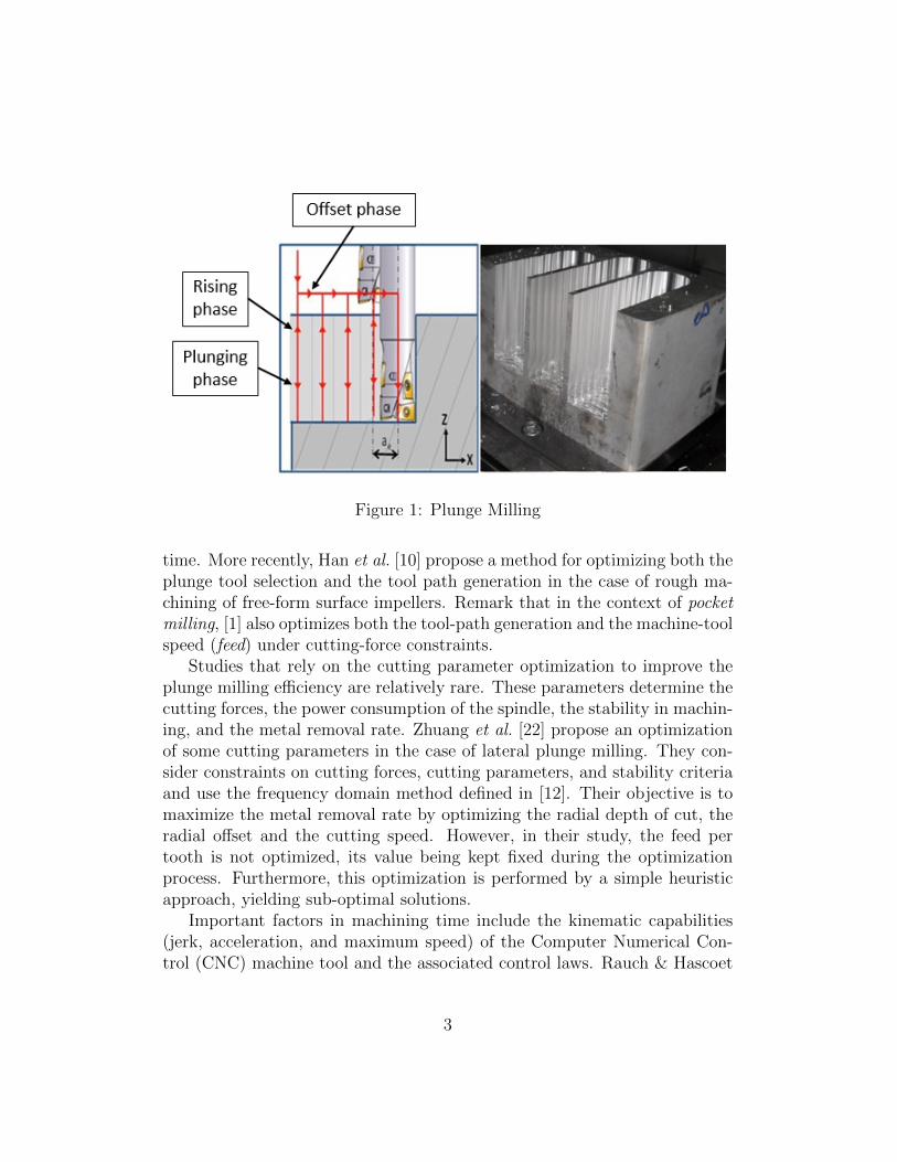
Figure 1: Plunge Milling

time. More recently, Han et al. [10] propose a method for optimizing both theplunge tool selection and the tool path generation in the case of rough ma-chining of free-form surface impellers. Remark that in the context of pocketmilling, [1] also optimizes both the tool-path generation and the machine-toolspeed (feed) under cutting-force constraints.

Studies that rely on the cutting parameter optimization to improve theplunge milling efficiency are relatively rare. These parameters determine thecutting forces, the power consumption of the spindle, the stability in machin-ing, and the metal removal rate. Zhuang et al. [22] propose an optimizationof some cutting parameters in the case of lateral plunge milling. They con-sider constraints on cutting forces, cutting parameters, and stability criteriaand use the frequency domain method defined in [12]. Their objective is tomaximize the metal removal rate by optimizing the radial depth of cut, theradial offset and the cutting speed. However, in their study, the feed pertooth is not optimized, its value being kept fixed during the optimizationprocess. Furthermore, this optimization is performed by a simple heuristicapproach, yielding sub-optimal solutions.

Important factors in machining time include the kinematic capabilities(jerk, acceleration, and maximum speed) of the Computer Numerical Con-trol (CNC) machine tool and the associated control laws. Rauch & Hascoet

3

present in [16] the impact of these factors, and also an analysis of the perfor-mances of plunge milling as a function of both the machine-tool kinematicscapabilities and of one specific control law. Despite the relevance of thesefactors in machining performances, none of the above approaches optimizessimultaneously all the major cutting parameters under kinematic constraints.Moreover, to the authors’ knowledge, no work on cutting parameter optimiza-tion takes into account the lengths of the tool trajectories.

In this paper, we propose a new methodology for optimizing the cut-ting parameters in order to minimize the plunge milling time. We considerthe case of full-slot plunge milling, to mill deep workpieces (casings), likeaeronautical pockets. This is the most critical case in terms of cutting forcesacting on the tool, as this is the situation where the cutting forces reach theirmaximum values [5]. Furthermore, since the cutting width (and therefore,the radial depth of cut) is equal to the tool diameter, one can see that in full-slot plunge milling the main cutting parameters to optimize are the cuttingspeed, the feed per tooth, and the radial offset. Note that the methodologyproposed in the present work can straightforwardly be extended to lateralplunge milling, simply by taking into account the radial depth of cut insteadof the tool diameter to determine the maximum cutting forces acting on thetool.

In the present study, machining capabilities, geometry tool selection (di-ameter, length and number of teeth), and tool path trajectories are supposedto be given (either from manufacturers, from the previously-mentioned meth-ods, or from commercial software).

The optimization methodology to optimize cutting parameters that wepropose has the following key novelties. It is based on mixed-integer non-linear programming, where we optimize, among the cutting parameters, thenumber of plunges, treated as an integer variable. This is in contrast withconsidering, as it is usually done, the radial offset, that is a real number(and should then be associated to a continuous variable). Thanks to theoptimization of the (integer) number of plunges, we are able to decomposethe problem into a sequence of optimization subproblems, each of which cor-responds to an elementary tool trajectory. Standard approaches consider areal-number value for the radial offset that is common to all elementary tra-jectories, yielding thereby suboptimal solutions (cutting parameters foundare independent of the length of the tool trajectories). This is in contrast toour approach, where the length of each elementary trajectory is taken intoaccount. Hence, we can determine specific values of the cutting parameters,

4

tailored for each elementary trajectory. Another strength of the methodologyintroduced in this paper is the fact that control laws are taken into accountin both time-machining and kinematic constraints in the plunge milling pro-cess. Indeed control laws have a significant impact on the optimal cuttingparameter values.

We propose a mathematical formulation of the problem based on Mixed-Integer NonLinear Programming (MINLP) [2]. This permits to take intoaccount both the continuous optimization variables (cutting speed, feed pertooth) and the integer optimization variables (number of plunges). More-over, nonlinear constraints due to both the CNC machine tool and to thetool characteristics are directly taken into account by this formulation. Theyinclude constraints related to: the maximum acceleration, the maximum jerkability, the maximum speed along each axis during the three different phasesof a plunge-milling cycle, the control law behaviour, the maximum powermachining, the maximum cutting forces, and the cutting parameter bounds.The objective function of the MINLP optimization problem is the machiningtime, to be minimized. It is the sum of the total (over all cycles) plungingtime, rising time, and offset time. These times are function of the given tra-jectories, the cutting parameters and, of course, of the previously-mentionedconstraints. Once the formulation of the MINLP model is established, effi-cient MINLP solvers can be used to get optimal cutting parameters. Theusefulness of this approach for industrial applications is demonstrated onrepresentative test cases of engine housing.

This paper is organized as follows. Section 2 describes the plunge millingcontext and surveys the different factors that drive the process. These arerelated to the tool, the material, the workpiece and the machine-tool. Usingthese driving factors, Section 3 presents one of our main contributions: aformulation of the plunge milling time optimization problem via MINLP. InSection 4, we first propose the detailed analytical expressions of the objectiveand the constraint functions that define the plunge milling time minimizationproblem. Then, we report and discuss the results of numerical experiments onrepresentative engine housing test cases. Finally, Section 5 draws conclusions.

5

Nomenclature

- Decision variables:Vc cutting speed (m/min)fz feed per tooth (mm/rev/tooth)ae radial offset (mm)Np number of plunges

- Input parameters:L elementary trajectory length (mm)Lp plunging length (mm)Lr rising length (mm)Lo offset length (mm)T machining time (s)tp plunging time (s)tr rising time (s)to offset time (s)i label of an axis (i ∈ {x, y, z})Vf programmed feedrate (m/min)A(t) acceleration vector at time t (m.s−2)Amax maximum absolute value of A(t) (m.s−2)Vs(t) speed vector at time t (m/min) for the Soft control lawVb(t) speed vector at time t (m/min) for the Brisk control lawV maxs maximum value of Vs(t) (m/min)

V maxb maximum value of Vb(t) (m/min)

Z number of teethD tool diameter (mm)Pmax maximum machining power (kW)Fmaxt maximum tangential cutting force (N)

Fmaxr maximum radial cutting force (N)

Fmaxa maximum axial cutting force (N)

- Lower and upper bounds:PM maximum machining power upper bound (kW)FMt maximum tangential cutting force upper bound (N)

FMr maximum radial cutting force upper bound (N)

FMa maximum axial cutting force upper bound (N)

V Mf maximum axis speed reachable (m/min)

V MR maximum rapid speed (m/min)

AM maximum axis acceleration reachable (m.s−2)JM maximum axis jerk (m.s−3)ame , aMefmz , fM

z

V mc , V M

c

lower and upper bounds on the decision variables

6

2 Plunge milling process

In this section, for given tool path trajectories, we overview the differentfactors that drive the plunge milling process. These are related to the tool,the material, the workpiece and the machine-tool.

More precisely, we describe the cutting parameters, the different phasesof a plunge cycle, the machine-tool kinematic characteristics, the control lawsproviding the temporal evolution profiles of speed, acceleration and jerk, andthe cutting forces that act on the tool as well as determine the machiningpower. These elements will be used in the next section to formalize theoptimization problem of minimizing the plunge milling time.

2.1 Cutting parameters

The cutting parameters that influence plunge milling are the cutting speedVc, the feed per tooth fz, and the radial offset ae. The radial offset ae (Fig. 1)represents the distance between two successive plunges into the stock and istherefore directly related to the number of plunges. The cutting parametersVc and fz together with the tool parameters (the number of teeth Z and thetool diameter D) drive the programmed feedrate Vf , which is given by:

Vf =103VcfzZ

πD(1)

The cutting parameters Vc, fz and ae, influence the cutting forces duringthe machining. Among these three parameters, fz and ae mainly influencethe tool loading, and have the strongest impact on the preponderant cuttingforces [5].

2.2 Plunge milling phases

The plunge milling process involves performing successive plunge cycles intothe material. The three different phases of a cycle are the following (seeFig. 1). The plunging phase is the phase during which the tool removesmaterial while going down. It is performed with a targeted machining speed,or programmed feedrate, noted Vf (depends on the cutting parameters). Dur-ing the rising phase the tool goes up. This phase is carried out in rapid

7

motion. Finally, during the offset phase the tool moves (above the work-piece), along the trajectory, so as to make an overlapping cut at the nextcycle. This phase is also carried out in rapid motion. All of these threephases are performed at different lengths (Lp, Lr, Lo, illustrated on Fig. 2).

Figure 2: Lengths, Lp, Lr, Lo, of the different phases of a plunge-millingcycle

2.3 Kinematic characteristics

The machine-tool capabilities to reach the targeted speed and the rapid speeddepend both on the machine kinematic characteristics and on the controllaws.

The kinematic characteristics are specific to a selected machine and giveconstraints on speed, acceleration and jerk. They are characterized by thefollowing values:

• V MRi , the upper bound on the maximum reachable rapid speed on thei-axis (i ∈ {x, y, z}) during the rising and offset phases

• V Mfi , the upper bound on the maximum reachable programmed feedrate

on the i-axis during the plunging phase

• AMi , the upper bound on the i-axis for the acceleration A(t) of the

machine at time t

8

• JMi , the upper bound on the i-axis jerk of the machine

2.4 Control laws

The control laws provide the temporal evolution profiles of speed, acceler-ation, and jerk of each axis i of the machine, subject to the above upperbounds (kinematic constraints). The programmed feedrate and the rapidmotion speed may be reached more or less rapidly following the control lawtemporal profiles. Although our optimization methodology can be appliedin the context of any type of control laws, the tests presented in this paperuse the jerk, acceleration and velocity profiles of the Siemens 840D CNCcontroller: they will be named “Brisk” and “Soft” laws in the sequel of thepaper (Fig. 3) [19].

For machining accuracy and workpiece quality reasons, the Soft law isused in the plunging phase. Using the Soft law, the axis motions are drivenby constant jerk steps (Fig. 3). Then, the acceleration temporal behaviour isdeduced. Finally, the Soft law provides the temporal evolution of the speedVs(t) (whose target value is the feedrate Vf ).

During the rising and offset phases, the Brisk law is applied (Fig. 2). Us-ing the Brisk law, the axis motions are driven by constant acceleration steps(Fig. 3). Then, the Brisk law provides the temporal evolution of the rapidspeed Vb(t) (whose target value is V M

R ).

The speed profile control laws can be represented by a piecewise polyno-mial function of time. For the Soft law (plunging phase), the feedrate profileis described by at most 7 phases (see Fig. 3):

Vs(t) =7∑

j=1

P js (t) (2)

where

P js (t) =

{aj + bjt+ cjt

2 if tj−1 6 t 6 tj (j = 1, .., 7)0 otherwise

(3)

For each axis i ∈ {x, y, z}, the coefficients aj, bj, cj are computed from AMi ,

JMi , Lp and the programmed feedrate Vf , which is a function of Vc, fz, D,

and Z. Note that Vs(t) 6 Vf 6 V Mf .

9

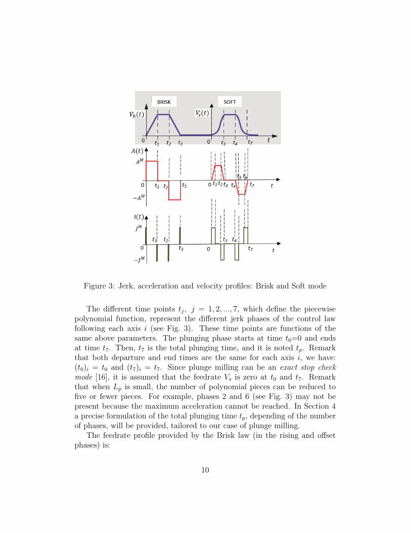
Figure 3: Jerk, acceleration and velocity profiles: Brisk and Soft mode

The different time points tj, j = 1, 2, ..., 7, which define the piecewisepolynomial function, represent the different jerk phases of the control lawfollowing each axis i (see Fig. 3). These time points are functions of thesame above parameters. The plunging phase starts at time t0=0 and endsat time t7. Then, t7 is the total plunging time, and it is noted tp. Remarkthat both departure and end times are the same for each axis i, we have:(t0)i = t0 and (t7)i = t7. Since plunge milling can be an exact stop checkmode [16], it is assumed that the feedrate Vs is zero at t0 and t7. Remarkthat when Lp is small, the number of polynomial pieces can be reduced tofive or fewer pieces. For example, phases 2 and 6 (see Fig. 3) may not bepresent because the maximum acceleration cannot be reached. In Section 4a precise formulation of the total plunging time tp, depending of the numberof phases, will be provided, tailored to our case of plunge milling.

The feedrate profile provided by the Brisk law (in the rising and offsetphases) is:

10

Vb(t) =3∑

j=1

P jb (t), (4)

where

P jb (t) =

{dj + ejt if tj−1 6 t 6 tj (j = 1, 2, 3)0 otherwise

(5)

For each axis i ∈ {x, y, z}, the coefficients dj and ej are function of AMi ,

Lr (or Lo) and of the rapid speed V MRi . Note that Vb(t) 6 V M

Ri .The different time points tj that define the piecewise linear function rep-

resent the different acceleration phases of the control law following each axis.The rising (or offset) phase starts at time t0=0, and ends at time t3. Remarkthat t3 is equal to tr (respectively, to), i.e. the rising (respectively, offset)duration. Both departure and end times are the same for each axis i. It isassumed that the feedrate Vb is zero at times t0 and t3. When Lr (respec-tively, Lo) is small, the number of linear pieces is reduced to two pieces. Inthis case, phase 2 does not exist. In Section 4 a precise formulation of thedurations tr and to, depending of the number of phases, will be provided.

The strong impact of control laws on machining time is illustrated in A.

2.5 Cutting forces and machining power

Beside the importance of kinematic and control law characteristics for com-puting accurate time machining, cutting forces have to be evaluated for en-suring tool safe life and to enforce machine power limitation.

The maximum cutting forces acting on the tool are the maximum tan-gential force Fmax

t , the maximum radial force Fmaxr , and the maximum axial

force Fmaxa . Generally, the tangential force is expressed as the product of a

specific cutting pressure and the instantaneous chip cross-section [4, 9, 13].Since the cutting pressure and the chip cross-section are both nonlinearly de-pendant on the cutting parameters, the maximum tangential force Fmax

t canbe expressed as a nonlinear function of Vc, fz, ae: F

maxt (Vc, fz, ae) [4, 5, 23].

The radial force is taken proportional to the tangential force [21], just as theaxial force. Then, the maximum radial and axial forces are again nonlinearfunctions of Vc, fz and ae: F

maxr (Vc, fz, ae) and Fmax

a (Vc, fz, ae).Due to both tool limitations (bending, stiffness, vibrations, wear, ...) and

maximum loading on machine-tool axis, these forces have to be below criticalvalues: Fmax

t (fz, Vc, ae) 6 FMt , Fmax

r (fz, Vc, ae) 6 FMr , Fmax

a (fz, Vc, ae) 6

11

FMa where FM

t , FMr , FM

a are respectively the upper bounds on the maximumallowable tangential, radial and axial cutting force. Concerning the maximummachining power, noted Pmax, it can be approximated by the product of themaximum tangential force Fmax

t and the cutting speed Vc, that is: Pmax 'Fmaxt Vc. It has to be below an upper bound value, generally given by the

machine tool: Pmax 6 PM .

3 Optimization formulation

In this section, we present our contribution on plunge milling optimizationthrough a mixed-integer nonlinear programming formulation. The aim isto propose optimized cutting parameter values that take into account thelengths of the tool trajectories, the machine-tool performances and limita-tions (kinematic characteristics, control laws, maximum machining power)and the tool characteristics. We consider that the machining capabilities(AM , JM ,V M

f ), the tool characteristics (D, Z, and its length), the lengthLp of the workpiece, and the tool path trajectory lengths are given. Tooltrajectories are defined by successive elementary tool paths such as: straightlines, arc circles and polynomial curves. In this paper, we decompose theoptimization of the total machining time into independent optimization sub-problems, each of which corresponds to an elementary tool path. Then, theglobal solution is obtained by assembling the solutions (the cutting param-eter values) of these subproblems. This permits to propose specific optimalcutting parameter values tailored to each elementary trajectory. Comparedto optimized cutting parameter taking the same values for all elementarytrajectories, this leads to a solution that is more time efficient for machiningthe workpiece. Consequently, in this section we present an optimization for-mulation for an elementary tool path with a given length, L.

We propose a mathematical formulation of the problem at hand underthe form of an optimization problem, and more precisely of a mixed-integernonlinear programming (MINLP) problem. Nonlinearities arise from theunderlying physical process. We propose a formulation involving continuousas well as integer optimization variables. The integer variables come fromthe discrete number of plunges and from modeling piecewise-defined functionsdue to the control laws that impact the machining time. To address these

12

difficulties, we take advantage of recent advances in MINLP [14].The optimization variables are: the cutting parameters (Vc, fz, ae) and

the number of plunges Np. The number of plunges, Np, is bounded to beinteger-valued (integer number of plunges for the given length of an elemen-tary trajectory). Moreover, there is a direct relationship between the numberof plunges and the radial offset ae:

Np = L/ae. (6)

Therefore, the optimization variables can in fact be reduced to: Vc, fz, Np

(and ae will be straightforwardly deduced from equation (6) after optimiza-tion). The first two variables (Vc, fz) are continuous and the last one, Np,is integer. Remark that common practice [11, 22] optimizes over the threecontinuous variables Vc, fz, ae, resulting in a value of Np that is not integer-valued and must be rounded to the next integer. This leads to an extraplunge which is likely to be inefficient. This loss of efficiency is summed upfor each elementary trajectory, clearly yielding to a suboptimal solution.For the sake of simplicity, and because the proposed formulation can easilybe extended, we assume that:

- the characteristics of each axis (x, y, z) are the same: we denote, fori ∈ {x, y, z}, AM

i = AM , Amaxi = Amax, V M

fi = V Mf and V M

Ri = V MR ;

- the length, Lr, of the rising phases and that, Lp, of the plunging phasesare equal and these phases involve only the z-axis;

- the length, Lo, of the offset phases is equal to the radial offset ae:Lo = ae;

- all of these lengths are constant along a given elementary trajectory.

3.1 Objective function

The objective function to be minimized is the machining time which can beexpressed as:

T (Vc, fz, Np) = Np (tp(Vc, fz) + tr + to(Np)) , (7)

where the plunging time, tp, the rising time, tr, and the offset time, to,functions are described in the next subsections.

13

3.1.1 Plunging time, tp

We define the plunging time as

tp(Vc, fz) =

tp1(Vc, fz), if V max

s (Vc, fz) = Vf (Vc, fz) and Amax(Vc, fz) = AM

tp2(Vc, fz), if V maxs (Vc, fz) = Vf (Vc, fz) and Amax(Vc, fz) < AM

tp3(Vc, fz), if V maxs (Vc, fz) < Vf (Vc, fz) and Amax(Vc, fz) = AM

tp4(Vc, fz), if V maxs (Vc, fz) < Vf (Vc, fz) and Amax(Vc, fz) < AM ,

(8)where:

• V maxs is the maximum speed that can be reached following the Soft

control law. It is a function of the given data: Lp, JM , AM , D, Z,

and of the optimization variables Vc, fz. Obviously, we always have0 6 V max

s (Vc, fz) 6 Vf (Vc, fz).

• Vf is a function of the given data, D, Z, and of the optimization vari-ables Vc, fz.

• Amax is a function of JM and Vf . Obviously, we always have 0 6Amax(Vc, fz) 6 AM .

Since Lp, JM , AM , D, Z are given data, the above quantities are only function

of the two optimization variables: Vc, fz. The expression of Vf (Vc, fz) is givenin equation (1). The analytic formulas that enable to compute tp(Vc, fz),V maxs (Vc, fz), and Amax(Vc, fz) will be provided in section 4 because these

functions depend on the selected control law.

To summarize,

• tp1 represents the plunging time associated with a displacement lengthLp when the maximum feedrate V max

s reaches Vf and the maximumacceleration Amax reaches AM .


s reaches Vf and the maximumacceleration Amax is below AM .


s is below Vf and the maximumacceleration Amax reaches AM .

14


s is below Vf and the maximumacceleration Amax is below AM .

3.1.2 Rising time, tr

The rising time is given by:

tr =

{tr1, if V max

b = V MR

tr2, if V maxb < V M

R ,(9)

where:

• tr1 represents the rising time associated with a displacement lengthLr = Lp, when the (given) rapid speed, V M

R , is reached.

• tr2 is the rising time when V maxb is below V M

R . Both tr1 and tr2 areindependent of the optimization variables.

• V maxb is the maximum speed that can be reached following the Brisk

control law. It is a function of the rising length, Lr, and of the max-imum acceleration reachable, AM : V max

b = ϕ(AM , Lr), where ϕ is afunction that is known. Since Lr and AM are given data, V max

b doesnot depend upon the optimization variables, therefore V max

b = κ, whereκ is a constant in the optimization problem. Note that V max

b is alwaysbelow V M

R : 0 6 V maxb = κ 6 V M

R . The analytic formulas that permitto compute tr, V

maxb , and thereby tr, will be provided in the test cases

presented in Section 4.

3.1.3 Offset time, to

The offset time, to, could also be defined in a piecewise manner, as for therising time (equation (9)). However, since the displacement length, Lo =ae = L/Np, is always sufficiently small due to technological constraints, thecondition V max

b = V MR is never met. The analytic formulas that enable to

compute to will be provided in Section 4.

15

3.2 Constraints

There are two distinct sets of constraints. First, there are disjunctive con-straints that allow to model the piecewise-defined functions that appear inthe objective function; second, those that model the physics of the system.

3.2.1 Disjunctive constraints

The definition of the objective function involves disjunctions as shown byequations (8) and (9). More precisely, T is a continuous piecewise-definedfunction of the optimization variables Vc, fz, and Np. Optimization softwarecannot handle directly problems involving piecewise-defined functions. In or-der to obtain a proper mathematical programming formulation, i.e. involvingonly differentiable functions (without any piecewise-defined functions), weintroduce the following binary variables:

• u1, u2, u3, and u4 for the plunging-time function, tp

• v for the rising-time function, tr

Using these variables, we can rewrite the piecewise-defined equation (9) as:

tr = vtr1 + (1− v)tr2, (10)

provided that the following constraints are taken into account:

v ∈ {0, 1} (11){0 6 V M

R − κ 6 (1− v)V MR

V maxb − V M

R < v.(12)

Indeed, one can easily verify, by enumerating the two possible values for v,that equation (9) is equivalent to equations (10), (11) and (12).

In an analogous manner, one can show that the piecewise-defined equa-tion (8) can be rewritten as

tp(Vc, fz) = u1tp1(Vc, fz) + u2tp2(Vc, fz) + u3tp3(Vc, fz) + u4tp4(Vc, fz) (13)

provided that the following constraints are taken into account:

u1, u2, u3, u4 ∈ {0, 1}

16

4∑j=1

uj = 1 (14)

0 6 Vf (Vc, fz)− V maxs (Vc, fz) 6 (1− u1)Vf (Vc, fz)

0 6 AM − Amax(Vc, fz) 6 (1− u1)AM


Amax(Vc, fz)− AM < (1− u2)V maxs (Vc, fz)− Vf (Vc, fz) < (1− u3)

0 6 AM − Amax(Vc, fz) 6 (1− u3)AM

V maxs (Vc, fz)− Vf (Vc, fz) < (1− u4)Amax(Vc, fz)− AM < (1− u4)

(15)

This can easily be verified by enumerating the four possible values for thevector (u1, u2, u3, u4): (1, 0, 0, 0), (0, 1, 0, 0), (0, 0, 1, 0) and (0, 0, 0, 1).

Finally, using equations (10) and (13), the objective function (7) becomes:

T (Vc, fz, Np) = Np

(u1tp1(Vc, fz) +u2tp2(Vc, fz) +u3tp3(Vc, fz) +u4tp4(Vc, fz)+

vtr1 + (1− v)tr2 + to(Np)).

Remark that constraints (12) and (15) involve strict inequalities, whichcannot be handled by mathematical programming solvers. Therefore, wechange strict into large inequalities after subtracting a sufficiently small (user-defined) constant ε from the right-hand-sides:


0 6 AM − Amax(Vc, fz) 6 (1− u1)AM


Amax(Vc, fz)− AM ≤ (1− u2)− εV maxs (Vc, fz)− Vf (Vc, fz) ≤ (1− u3)− ε

0 6 AM − Amax(Vc, fz) 6 (1− u3)AM

V maxs (Vc, fz)− Vf (Vc, fz) ≤ (1− u4)− εAmax(Vc, fz)− AM ≤ (1− u4)− ε

(16)

and {0 6 V M

R − κ 6 (1− v)V MR

V maxb − V M

R ≤ v − ε(17)

17

3.2.2 Cutting parameter bounds

Due to material and tool characteristics, cutting parameters have to satisfythe following lower-bound and upper-bound inequalities:

V mc 6 Vc 6 V M

c (18)

fmz 6 fz 6 fM

z (19)

ame 6 ae 6 aMe (20)

where V mc , V M

c , fmz , f

Mz , ame , a

Me are given data (depending upon the material

and the machine features). Remark that the last equation is equivalent to

L

aMe≤ Np ≤

L

ame(21)

since Np =L

ae.

3.2.3 Machine kinematics

The kinematic characteristics of the machine tool imply the following in-equalities:

• The programmed feedrate, Vf , has to be smaller than V Mf : Vf (Vc, fz) 6

V Mf .

• The maximum acceleration, Amax, has to be smaller thanAM : Amax(Vc, fz) 6AM .

3.2.4 Cutting forces

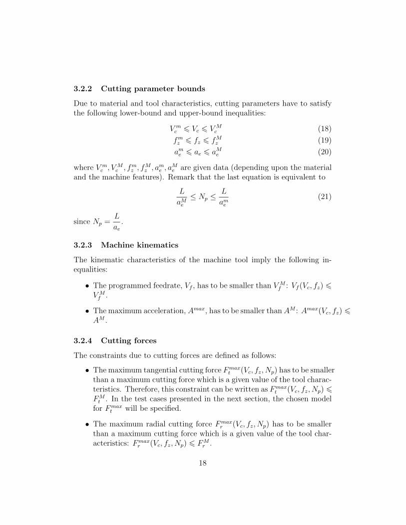
The constraints due to cutting forces are defined as follows:

• The maximum tangential cutting force Fmaxt (Vc, fz, Np) has to be smaller

than a maximum cutting force which is a given value of the tool charac-teristics. Therefore, this constraint can be written as Fmax

t (Vc, fz, Np) 6FMt . In the test cases presented in the next section, the chosen model

for Fmaxt will be specified.

• The maximum radial cutting force Fmaxr (Vc, fz, Np) has to be smaller

than a maximum cutting force which is a given value of the tool char-acteristics: Fmax

r (Vc, fz, Np) 6 FMr .

18

• The maximum axial cutting force Fmaxa (Vc, fz, Np) has to be smaller

than a maximum cutting force which is a given value of the tool andthe machine-tool characteristics: Fmax

a (Vc, fz, Np) 6 FMa .

• The maximum power associated with cutting can be approximated byPmax ' Fmax

t (Vc, fz, Np)Vc. The maximum power has to be smallerthan the given maximum machining power PM . Therefore this con-straint can be written as Pmax(Vc, fz, Np) 6 PM .

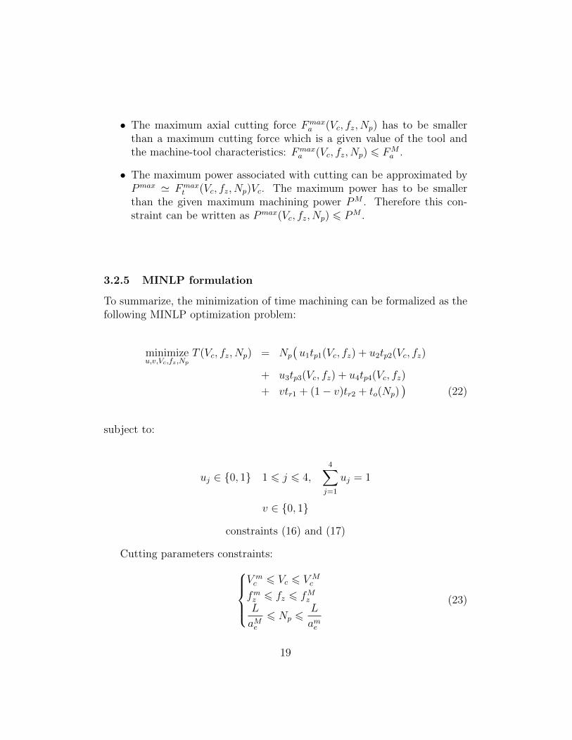
3.2.5 MINLP formulation

To summarize, the minimization of time machining can be formalized as thefollowing MINLP optimization problem:

minimizeu,v,Vc,fz ,Np

T (Vc, fz, Np) = Np

(u1tp1(Vc, fz) + u2tp2(Vc, fz)

+ u3tp3(Vc, fz) + u4tp4(Vc, fz)

+ vtr1 + (1− v)tr2 + to(Np))

(22)

subject to:

uj ∈ {0, 1} 1 6 j 6 4,4∑

j=1

uj = 1

v ∈ {0, 1}

constraints (16) and (17)

Cutting parameters constraints:V mc 6 Vc 6 V M

c

fmz 6 fz 6 fM

z

L

aMe6 Np 6

L

ame

(23)

19

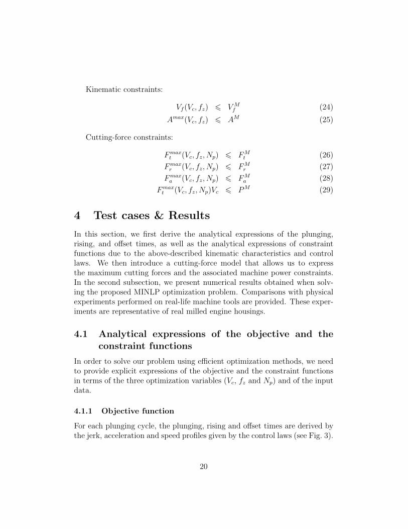
Kinematic constraints:

Vf (Vc, fz) 6 V Mf (24)

Amax(Vc, fz) 6 AM (25)

Cutting-force constraints:

Fmaxt (Vc, fz, Np) 6 FM

t (26)

Fmaxr (Vc, fz, Np) 6 FM

r (27)

Fmaxa (Vc, fz, Np) 6 FM

a (28)

Fmaxt (Vc, fz, Np)Vc 6 PM (29)

4 Test cases & Results

In this section, we first derive the analytical expressions of the plunging,rising, and offset times, as well as the analytical expressions of constraintfunctions due to the above-described kinematic characteristics and controllaws. We then introduce a cutting-force model that allows us to expressthe maximum cutting forces and the associated machine power constraints.In the second subsection, we present numerical results obtained when solv-ing the proposed MINLP optimization problem. Comparisons with physicalexperiments performed on real-life machine tools are provided. These exper-iments are representative of real milled engine housings.

4.1 Analytical expressions of the objective and theconstraint functions

In order to solve our problem using efficient optimization methods, we needto provide explicit expressions of the objective and the constraint functionsin terms of the three optimization variables (Vc, fz and Np) and of the inputdata.

4.1.1 Objective function

For each plunging cycle, the plunging, rising and offset times are derived bythe jerk, acceleration and speed profiles given by the control laws (see Fig. 3).

20

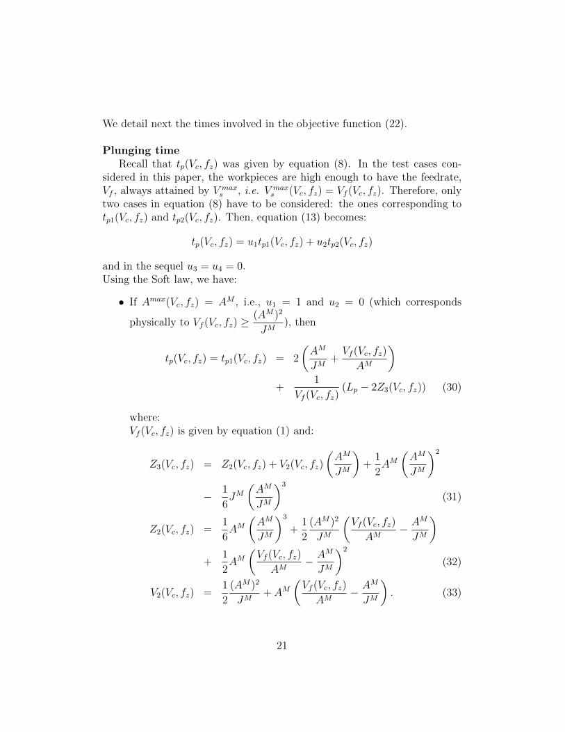
We detail next the times involved in the objective function (22).

Plunging timeRecall that tp(Vc, fz) was given by equation (8). In the test cases con-

sidered in this paper, the workpieces are high enough to have the feedrate,Vf , always attained by V max

s , i.e. V maxs (Vc, fz) = Vf (Vc, fz). Therefore, only

two cases in equation (8) have to be considered: the ones corresponding totp1(Vc, fz) and tp2(Vc, fz). Then, equation (13) becomes:

tp(Vc, fz) = u1tp1(Vc, fz) + u2tp2(Vc, fz)

and in the sequel u3 = u4 = 0.Using the Soft law, we have:

• If Amax(Vc, fz) = AM , i.e., u1 = 1 and u2 = 0 (which corresponds

physically to Vf (Vc, fz) ≥(AM)2

JM), then

tp(Vc, fz) = tp1(Vc, fz) = 2

(AM

JM+Vf (Vc, fz)

AM

)+

1

Vf (Vc, fz)(Lp − 2Z3(Vc, fz)) (30)

where:Vf (Vc, fz) is given by equation (1) and:

Z3(Vc, fz) = Z2(Vc, fz) + V2(Vc, fz)

(AM

JM

)+

1

2AM

(AM

JM

)2

− 1

6JM

(AM

JM

)3

(31)

Z2(Vc, fz) =1

6AM

(AM

JM

)3

+1

2

(AM)2

JM

(Vf (Vc, fz)

AM− AM

JM

)+

1

2AM

(Vf (Vc, fz)

AM− AM

JM

)2

(32)

V2(Vc, fz) =1

2

(AM)2

JM+ AM

(Vf (Vc, fz)

AM− AM

JM

). (33)

21

• If Amax(Vc, fz) < AM , i.e., u1 = 0 and u2 = 1 (which corresponds

physically to Vf (Vc, fz) <(AM)2

JM), then

tp(Vc, fz) = tp2(Vc, fz) = 2

(Amax(Vc, fz)

JM+

Vf (Vc, fz)

Amax(Vc, fz)

)+Lp − 2Z3(Vc, fz)

Vf (Vc, fz)(34)

where:

Amax(Vc, fz) =√JMVf (Vc, fz) (35)

Z3(Vc, fz) = Z2(Vc, fz) + V2(Vc, fz)

(Amax(Vc, fz)

JM

)+

1

2Amax(Vc, fz)

(Amax(Vc, fz)

JM

)2

−1

6JM

(Amax(Vc, fz)

JM

)3

(36)

Z2(Vc, fz) =1

6Amax(Vc, fz)

(Amax(Vc, fz)

JM

)3

+1

2

((Amax(Vc, fz))

2

JM

)(Vf (Vc, fz)

Amax(Vc, fz)− Amax(Vc, fz)

JM

)+

1

2Amax(Vc, fz)

(Vf (Vc, fz)


JM

)2

(37)

V2(Vc, fz) =1

2

((Amax(Vc, fz))

2

JM

)+ Amax(Vc, fz)

(Vf (Vc, fz)


JM

). (38)

Rising timeRecall that tr was given by equation (9). In most CNC machine tools

actually used in industry, the rapid speed V MR is so high that in practice it

can rarely be attained. Therefore, only one case has to be considered: theone corresponding to tr2. Then equation (10) becomes:

tr = tr2

and v = 0 in our tests. Using the Brisk law, we get:

tr = tr2 = 2

√Lr

AM. (39)

22

Offset timeRecall that (see subsection 3.1.3) the rapid speed V M

R cannot be reachedduring the offset phase. Since the Brisk law is applied again, we obtain the

same formula as for the rising phase, by replacing the length Lr withL

Np

:

to(Np) = 2

√L

NpAM(40)

4.1.2 Constraint functions

There are two groups of constraints that remain to be made explicit.

KinematicsUsing equations (1) and (35), the kinematic constraints (24) and (25) are

obtained as follows:

103VcfzZ

πD≤ V M

f√JM

103VcfzZ

πD≤ AM

Cutting forcesThere are several mechanistic models for cutting forces in the literature,

as for example [4, 5, 23]. All of these models are relevant to our optimiza-tion problem. For validating our methodology, we use the mechanistic modelof [4], which is applied on the material Al356 alloy, plunge milled with aSandvik tool referenced as R210-025A20-09M. This model gives the analyti-cal formulas of cutting forces to be used in constraints (26), (27), and (28).Based on this model, we propose the following expressions of the maximalcutting forces:

23

Fmaxt (Vc, fz, Np) = Fmax

t (fz, Np) = 325.17(cos(10◦)fz)−0.418 L

Np

fz (41)

Fmaxr (Vc, fz, Np) = Fmax

r (fz, Np) = 202.85(cos(10◦)fz)−0.418 L

Np

fz (42)

Fmaxa (Vc, fz, Np) = Fmax

a (fz, Np) = 130.33(cos(10◦)fz)−0.682 L

Np

fz (43)

Remark that these forces do not depend upon Vc, contrary for example tothe model proposed by Danis et al. [5] to plunge milling magnesium alloys.However, this is without loss of generality for our optimization methodology.

Finally, the maximal machining power constraint (29) is straightforwardlyobtained:

325.17(cos(10◦)fz)−0.418 L

Np

fzVc 6 PM (44)

4.2 Numerical results

All machining times reported throughout this section correspond to simu-lated machining times, computed following equations (30), (34), (39) and(40). In order to ensure consistency with real machining times, we performsome actual tests (physical experiments) on the CNC machine tool DMU85Monoblock with a Siemens 840D CNC controller. We observe that the dif-ference between simulated and real machining times always remains below6%. As it will be seen later, this is much lower than the gains obtained withour optimization methodology. This thereby validates the physical modelson which our optimization formulation relies. Numerical tests are carriedout using the same material, A356 alloy, and the same plunge milling tool(Sandvik R210-Q25A20-09 M) as in [4].

The optimization problem we presented belongs to a class of problems(NP hard) known to be very difficult to solve, as it is nonlinear and involvesboth continuous and integer variables. The optimization model we propose isimplemented in AMPL modeling language [8], and the optimization problemis solved using the state-of-the-art solver COUENNE [2] for Mixed-IntegerNonlinear Problems (MINLP). The default setting is used. In order to be ableto use such an efficient global optimization solver, we replace equations (41),(42), and (43) with a rational-function model that fits very accurately theseequations on the relevant definition domain.

24

Tests with the above optimization software were performed on a 2.66 GHzIntel Xeon (octo core) processor with 32 GB of RAM and Linux OperatingSystem. To give a rough idea, one complete run of the optimization (on onetest problem) involves between 0.23 and 0.56 seconds of CPU time. Recallthat one run involves one elementary trajectory. Therefore, a complete man-ufacturing of one workpiece will require to sum up this computing time overall elementary trajectories.

We present below eight test cases, each of which is followed by the resultsobtained after optimization. These tests are performed varying tool charac-teristics, the machine power and kinematics, the cutting-force constraints aswell as the workpiece characteristics (the main variations are emphasized inbold characters in the tables below). These tests give an overview of realcases that can be met in practice on milled engine housings. In all tests, wekeep constant: the tool diameter (D), the length of the elementary trajectory(L), the maximum machine power upper bound (PM) and the lower and up-per bounds of the decision variables. These values are displayed in Table 1.The maximum machine power is set at a large value so as to improve therange of possible values for the cutting parameters. The optimization resultsare compared with a standard industrial setting (SIS), based on engineeringknow-how in such a way to satisfy the constraints on cutting parameters,kinematics and cutting forces, while ensuring good machining time perfor-mance. More precisely, the following procedure is applied. The values ofVc, fz, and ae are chosen as high as possible so as to fulfill the constraints.The three values are defined sequentially by using a trial-and-error approach.First, ae is taken close to the upper bound aMe , then the value of fz is deducedfrom the cutting force model, and finally, the value of Vc follows from theother constraints. The number of plunges, Np, is simply obtained by round-ing above the ratio L/ae. This is in contrast with the MINLP approachwhich computes optimal values for Vc, fz, Np, where Np is constrained to beinteger. The value of ae is then simply deduced from (6).

We use the above-mentioned DMU85 machine and two other (more per-forming) machines, presented in [16].

For the sake of simplicity, among the three cutting-force constraints (26)-(28), only the first one (equation (26)) is taken into account (and we observeda posteriori that the two other constraints are not violated at the solutionfound).

We next present the results for the eight test cases. For each approach(SIS and MINLP) we report: the values of the variables, Vc, fz, Np and ae;

25

Table 1: Values of the parameters that are kept constant throughout thetests

parameter D L PM V mc V M

c

units mm mm kW m/min m/min

value 25 200 20 200 1250

parameter fmz fM

z ame aMeunits mm/rev/tooth mm/rev/tooth mm mm

value 0.05 1 0.5 8

the three plunging-phase times, tp, tr and to; the total machining time, T , forone elementary trajectory. Finally the last column of the tables reports therelative gain of MINLP over SIS total machining time.

The first test (Table 2) considers the standard CNC machine tool DMU85Monoblock with a high value of FM

t so that the tool load is not much con-strained.

Table 2: Test 1: input dataparameter Lp AM JM V M

R V Mf FM

t

units mm m/s2 m/s3 m/min m/min Nvalue 75 6 40 40 40 900

Table 3 displays the results obtained after optimization compared with thestandard industrial setting (SIS) procedure described above. One observesthat for one given elementary trajectory, the optimization results are better,but close to the one obtained by SIS. Note that the SIS solution provides anon-integer value of L/ae = 26.67 which was then rounded up to 27 in orderto obtain a feasible number of plunges.

The second test (Table 4) considers the same machine as for Test 1, butTest 2 involves a lower value of FM

t so as to reduce the bending and/orthe vibrations of the tool. The input value for FM

t is chosen taking intoaccount the relation between the deflection of the tool, the cutting forcesand experience of practitioners.

26

Table 3: Test 1: optimization resultsVc fz Np ae tp tr to T gain

units m/min mm/rev/tooth mm s s s s %

SIS 1250 0.194 27 7.50 0.85 0.22 0.071 30.80

MINLP 1250 0.198 27 7.41 0.83 0.22 0.070 30.45 1.1


R V Mf FM

t

value 75 6 40 40 40 600

The MINLP solution of Table 5 increases the number of plunges withrespect to the SIS solution (going from 27 to 39) and thereby decreases theradial offset (ae) from 7.5 down to 5.13. Moreover, the feed per tooth, fz,increases from 0.087 to 0.182 and the cutting speed, Vc, remains constant.Thus, the optimized process allows one to perform more plunges at a higherspeed. The gain in terms of machining time is above 15%. Here, one al-ready observes the benefit of the optimization which yields an interestingyet unpredictable result that is substantially different from the engineeringknow-how SIS methodology.


SIS 1250 0.087 27 7.50 1.70 0.22 0.071 53.96MINLP 1250 0.182 39 5.13 0.89 0.22 0.058 45.69 15.3

Test 3 (Table 6) involves a higher workpiece (higher value of Lp), all otherconditions remaining as for Test 2.


R V Mf FM

t

value 100 6 40 40 40 600

The optimization results of Table 7 show that the gain in machining timegrows further with a higher workpiece.

27


SIS 1250 0.087 27 7.50 2.25 0.26 0.071 69.52MINLP 1250 0.197 41 4.88 1.07 0.26 0.057 57.02 18.0

Let us now consider, in Test 4 (Table 8), an even higher workpiece. Thelength of the tool being increased, its stiffness thereby reduces and, as aconsequence, one must set a stricter cutting-force constraint (lower FM

t ) inorder to avoid bending and/or vibration of the tool.


R V Mf FM

t

value 125 6 40 40 40 500

As shown in Table 9, the gain obtained by the MINLP solution (over SIS)for Test 4 is substantial: the optimized process yields a very large number ofplunges (Np = 91, as opposed to 27 for SIS) at a very high programmed fee-drate, Vf = 31.826 m/min (from equation 1). The gain in terms of machiningtime is 41.8%.


SIS 1250 0.054 27 7.50 4.43 0.29 0.071 129.21MINLP 1250 1.00 91 2.20 0.50 0.29 0.038 75.20 41.8

Test 5 (Table 10) involves a high-performance machine, featuring a higher(compared with the previous tests) maximum axis acceleration reachable,AM . The other parameter values are the same as those of Test 2.

The optimization results (Table 11) show, when compared with those ofTest 2, an even higher gain (17.2% as compared with 15.3%).

Test 6 (Table 12) differs from Test 5 only in the value of the maximumaxis jerk reachable, JM , which is much increased. The other parameter valuesare the same as those of Test 2.

28


R V Mf FM

t

value 75 10 40 40 40 600


SIS 1250 0.087 27 7.50 1.70 0.17 0.055 52.17MINLP 1250 0.190 40 5.00 0.86 0.17 0.045 43.17 17.2


R V Mf FM

t

value 75 10 100 40 40 600

Table 13 reveals a further improvement in machining time, T . To sum-marize, when considering only the MINLP solutions of Tests 2, 5 and 6, oneremarks that increasing either AM or JM yields gains in machining times,more plunges and higher feedrates.


SIS 1250 0.087 27 7.50 1.68 0.17 0.055 51.39MINLP 1250 0.212 43 4.65 0.75 0.17 0.043 41.37 19.5

Recall that from Test 3 to Test 4, we increased Lp and therefore decreasedFMt to take stiffness into account. Test 7 (Table 14) comes back to the main

settings of Test 4 together with the high-performance machine of Tests 5 and6.

As shown on Table 15, the gain with respect to the engineering know-howSIS methodology is striking: 52.7%. When comparing the MINLP solutionsobtained for Tests 4 and 7 (that differs with respect to the performance ofthe machine), the gain goes from 41.8% to 52.7%. Thus, higher workpieces(and corresponding tool-stiffness constraints) conduct to better results.

29


R V Mf FM

t

value 125 10 100 40 40 500


SIS 1250 0.054 27 7.50 4.40 0.22 0.055 126.41MINLP 1250 1.00 91 2.20 0.40 0.22 0.030 59.79 52.7

Test 8 (Table 16) considers an even more performing machine tool: weuse the characteristics of a parallel kinematic machine presented in [16] forplunge milling. Its maximum acceleration value is AM=15 m.s−2 and V M

f =50m/min.


R V Mf FM

t

value 125 15 100 50 50 500

Table 17 displays a gain that continues to grow: 55.6%. When comparingthe optimization solutions obtained for Tests 4, 7 and 8 (in order of increasingperformance of the machine tool used), the gains are 41.8%, 52.7% and 55.6%.


SIS 1250 0.054 27 7.50 4.40 0.18 0.044 125.03MINLP 1250 1.00 91 2.20 0.40 0.18 0.024 55.56 55.6

5 Conclusions

We propose a mathematical formulation of the cutting-parameter optimiza-tion in plunge milling, taking into account the lengths of the tool trajecto-

30

ries, control laws and cutting forces. This formulation takes the form of anMINLP problem whose optimization variables include the (integer) numberof plunges.

The advantages of our approach over traditional machining optimizationis twofold. First, our method provides a specific set of cutting parameterstailored to each elementary trajectory, which, together, constitute the tooltrajectory. Second, for each elementary trajectory, our formulation yieldsequidistant plunges that are optimal with respect to all the cutting parame-ters. This is in contrast with standard machining optimization that uses onlycontinuous variables. Indeed, such standard approaches not only consider asame set of cutting parameters over the whole trajectory, but moreover ad-just a posteriori the number of plunges, while keeping fixed the values ofthe other cutting parameters, which is necessarily suboptimal. This loss ofefficiency is then summed up over all the elementary trajectories.

We present and discuss computational results, obtained through the useof modern general-purpose MINLP software, validated on CNC machines.The tests proposed cover a wide range of input parameter values (work-piece and tool characteristics, machine performances, and tool and machineconstraints). Our results emphasize the fact that optimal values of the cut-ting parameters are very sensitive to the various constraints (cutting-forceconstraints and maximal machining power) and are difficult to predict bystandard approaches. The more performing machine one uses, the betterresults our optimization methodology yields. Gains as high as 55% for high-performance machine tools are obtained when compared with standard in-dustrial setting based on engineering know-how.

Future research will extend this work by optimizing moreover both thetool choice and the associated tool-path trajectory. Moreover, one couldfocus on attempting to search for cutting-parameter values that are robustwith respect to uncertainty in input data.

A Impact of control laws on machining time

In this appendix, we show the strong impact of control laws on machiningtime, especially when high speeds are used. This is illustrated in differenttest cases by comparing real machining time and simulated machining timeprovided by CAM software that does not take into account the control laws.

For illustrating our purpose, we have performed plunge milling tests on a

31

DMU50 evolution 5-axis NC machine (with a Siemens 840D CNC controller),for which the machining times have been recorded. In commercial CAMsoftware, the kinematic machine-tool characteristics can be considered, butgenerally the control law profiles cannot be taken into account. To comparereal machining times with simulation times, two CAM software (CATIA V5and Delcam) have been used. The tests have been performed (Table 18)on different workpieces with the following kinematic characteristics: for i ∈{x, y, z}, V M

Ri = V MR = 50 m.min−1, V M

fi = V Mf = 24 m.min−1, JM

i =JM = 40 m.s−3, AM

i = AM = 4.9 m.s−2. For the first workpiece, CatiaV5 simulates the machining time equal to 91 s, compared to 235 s of realtime machining. For the second workpiece tested, Delcam has provided asimulation time of 86 s against 213.6 s of machining time. In these twoexamples, CAM software decreases the actual machining time by about 60%.Table 18 presents all the results of the time differences for various workpiecesand programmed feedrates. Errors are in the range [49%, 61%] for bothCAM software. Nevertheless, depending on the machine characteristics (V M

R ,V Mf , AM , JM), these errors vary significantly. These test results show the

criticity of the control laws for the computation of simulated machining times.Therefore, velocity profiles provided by control laws will be integrated intoour optimization model.

Catia V5 (s) Delcam (s) Time machining (s) errorsTest1 91 235 61%Test2 86 213.6 60%Test3 95 186 49%Test4 87 158 45%Test5 82 174.7 53%

Table 18: Comparison of machining time simulated by two CAM softwareand real time machining for different test cases

References

[1] A. Banerjee, H.-Y. Feng, and E. V. Bordatchev. Process planning forFloor machining of 2D pockets based on a morphed spiral tool pathpattern. Computers & Industrial Engineering, 63(4):971–979, 2012.

32

[2] P. Belotti, J. Lee, L. Liberti, F. Margot, and A. Wachter. Branchingand bounds tightening techniques for non-convex MINLP. OptimizationMethods and Software, 24(4-5):597–634, 2009.

[3] S. Calvel and M. Mongeau. Black-box structural optimization of a me-chanical component. Computers & Industrial Engineering, 53(3):514–530, 2007.

[4] A. Damir, E.-G. Ng, and M. Elbestawi. Force prediction and stabilityanalysis of plunge milling of systems with rigid and flexible workpiece.The International Journal of Advanced Manufacturing Technology, 54(9-12):853–877, 2010.

[5] I. Danis, F. Monies, P. Lagarrigue, and N. Wojtowicz. Cutting forces andtheir modelling in plunge milling of magnesium-rare earth alloys. The In-ternational Journal of Advanced Manufacturing Technology, 84(9):1801–1820, 2016.

[6] I. Danis, N. Wojtowicz, F. Monies, and P. Lagarrigue. Influence ofdry plunge milling conditions on surface integrity of magnesium alloys.International Journal of Mechatronics and Manufacturing Systems, 7(2-3):141–156, 2014.

[7] T. Finzer. High speed machining (HSC) of sculptured surfaces in dieand mold manufacturing. In G. J. Olling, B. K. Choi, and R. B. Jerard,editors, Machining Impossible Shapes, number 18 in IFIP – The Interna-tional Federation for Information Processing, pages 333–341. Springer,1999.

[8] R. Fourer and D. M. Gay. The AMPL Book. Duxbury Press, PacificGrove, 2002.

[9] P. Gilles, F. Monies, and W. Rubio. Optimum orientation of a torusmilling cutter: Method to balance the transversal cutting force. Inter-national Journal of Machine Tools and Manufacture, 47(15):2263–2272,2007.

[10] F. Y. Han, D. H. Zhang, M. Luo, and B. H. Wu. Optimal CNC plungecutter selection and tool path generation for multi-axis roughing free-form surface impeller channel. The International Journal of AdvancedManufacturing Technology, 71(9-12):1801–1810, 2014.

33

[11] H. Juan, S. F. Yu, and B. Y. Lee. The optimal cutting-parameter se-lection of production cost in HSM for SKD61 tool steels. InternationalJournal of Machine Tools and Manufacture, 43(7):679–686, 2003.

[12] J. H. Ko and Y. Altintas. Time domain model of plunge millingoperation. International Journal of Machine Tools and Manufacture,47(9):1351–1361, 2007.

[13] F. Koenigsberger and A. Sabberwal. An investigation into the cuttingforce pulsations during milling operations. International Journal of Ma-chine Tool Design and Research, 1(1):15–33, 1961.

[14] J. Lee and S. Leyffer. Mixed integer nonlinear programming, volume154. Springer Science & Business Media, 2011.

[15] K. Moussaoui, F. Monies, M. Mousseigne, P. Gilles, and W. Rubio.Balancing the transverse cutting force during inclined milling and effecton tool wear: application to Ti6al4v. The International Journal ofAdvanced Manufacturing Technology, 82(9):1859–1880, 2016.

[16] M. Rauch and J.-Y. Hascoet. Selecting a milling strategy with regard tothe machine tool capabilities: application to plunge milling. The Inter-national Journal of Advanced Manufacturing Technology, 59(1-4):47–54,2012.

[17] J. X. Ren, C. F. Yao, D. H. Zhang, Y. L. Xue, and Y. S. Liang. Re-search on tool path planning method of four-axis high-efficiency slotplunge milling for open blisk. The International Journal of AdvancedManufacturing Technology, 45(1-2):101–109, 2009.

[18] H. Schulz. High-speed machining. In A. I. Dashchenko, editor, Manufac-turing Technologies for Machines of the Future, pages 197–214. Springer,2003.

[19] Siemens. Technical Online-Documentation for SINUMERIK, SINAM-ICS and SIMOTICS - ID: 109476679 - Industry Support Siemens, 2015.

[20] C. Sun, Y. Wang, and N. Huang. A new plunge milling tool pathgeneration method for radial depth control using medial axis trans-form. The International Journal of Advanced Manufacturing Technology,76(9):1575–1582, 2015.

34

[21] J. Tlusty and P. MacNeil. Dynamics of cutting forces in end milling.Annals CIRP, 24:21–25, 1975.

[22] K. Zhuang, X. Zhang, D. Zhang, and H. Ding. On cutting parame-ters selection for plunge milling of heat-resistant-super-alloys based onprecise cutting geometry. Journal of Materials Processing Technology,213(8):1378–1386, 2013.

[23] K. Zhuang, X. Zhang, X. Zhang, and H. Ding. Force prediction inplunge milling of inconel 718. In C.-Y. Su, S. Rakheja, and H. Liu,editors, Intelligent Robotics and Applications, number 7507 in LectureNotes in Computer Science, pages 255–263. Springer Berlin Heidelberg,2012.

35

Plunge milling time optimization via mixed-integer ...

Documents

Transcript of Plunge milling time optimization via mixed-integer ...