Pixel-based image classification

Lecture 8

What is image classification or pattern recognition

Is a process of classifying multispectral (hyperspectral) images into patterns of varying gray or assigned colors that represent either clusters of statistically different sets of multiband data, some of which can be

correlated with separable classes/features/materials. This is the result of Unsupervised Classification, or

numerical discriminators composed of these sets of data that have been grouped and specified by associating each with a particular class, etc. whose identity is known independently and which has representative areas (training sites) within the image where that class is located. This is the result of Supervised Classification.

Spectral classesSpectral classes are those that are inherent in the remote sensor data and are those that are inherent in the remote sensor data and must be identified and then labeled by the analyst.must be identified and then labeled by the analyst.

Information classesInformation classes are those that human beings define. are those that human beings define.

supervised classification. Identify known a priori through a combination of fieldwork, map analysis, and personal experience as training sites; the spectral characteristics of these sites are used to train the classification algorithm for eventual land-cover mapping of the remainder of the image. Every pixel both within and outside the training sites is then evaluated and assigned to the class of which it has the highest likelihood of being a member.

unsupervised classification, The computer or algorithm automatically group pixels with similar spectral characteristics (means, standard deviations, covariance matrices, correlation matrices, etc.) into unique clusters according to some statistically determined criteria. The analyst then re-labels and combines the spectral clusters into information classes.

Hard vs. Fuzzy classification

Supervised and unsupervised classification algorithms typically use hard classification logic to produce a classification map that consists of hard, discrete categories (e.g., forest, agriculture).

Conversely, it is also possible to use fuzzy set classification logic, which takes into account the heterogeneous and imprecise nature (mix pixels) of the real world. Proportion of the m classes within a pixel (e.g., 10% bare soil, 10% shrub, 80% forest). Fuzzy classification schemes are not currently standardized.

Pixel-based vs. Object-oriented classification

In the past, most digital image classification was based on processing the entire scene pixel by pixel. This is commonly referred to as per-pixel (pixel-based) classification.

Object-oriented classification techniques allow the analyst to decompose the scene into many relatively homogenous image objects (referred to as patches or segments) using a multi-resolution image segmentation process. The various statistical characteristics of these homogeneous image objects in the scene are then subjected to traditional statistical or fuzzy logic classification. Object-oriented classification based on image segmentation is often used for the analysis of high-spatial-resolution imagery (e.g., 1  1 m Space Imaging IKONOS and 0.61  0.61 m Digital Globe QuickBird).

Knowledge-based information extraction: Artificial Intelligence

Neural network Decision tree Support vector machine (SVM) …

Purposes of classification

Land use and land cover (LULC)

Vegetation types

Geologic terrains

Mineral exploration

Alteration mapping

…….

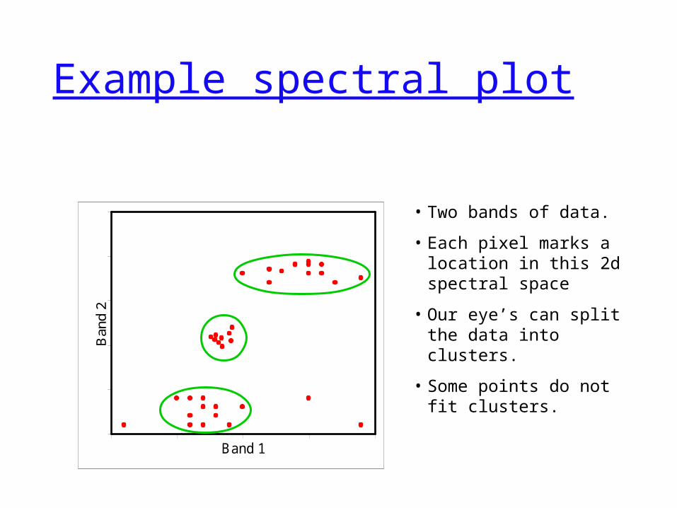
Example spectral plot

Band 1

Ban

d 2

• Two bands of data.

• Each pixel marks a location in this 2d spectral space

• Our eye’s can split the data into clusters.

• Some points do not fit clusters.

1. Unsupervised classification1. Unsupervised classification Uses statistical techniques to group n-dimensional data into their natural spectral

clusters, and uses the iterative procedures label certain clusters as specific information classes K-mean and ISODATA

For the first iteration arbitrary starting values (i.e., the cluster properties) have to be selected. These initial values can influence the outcome of the classification.

In general, both methods assign first arbitrary initial cluster values. The second step classifies each pixel to the closest cluster. In the third step the new cluster mean vectors are calculated based on all the pixels in one cluster. The second and third steps are repeated until the "change" between the iteration is small. The "change" can be defined in several different ways, either by measuring the distances of the mean cluster vector have changed from one iteration to another or by the percentage of pixels that have changed between iterations.

The ISODATA algorithm has some further refinements by splitting and merging of clusters. Clusters are merged if either the number of members (pixel) in a cluster is less than a

certain threshold or if the centers of two clusters are closer than a certain threshold. Clusters are split into two different clusters if the cluster standard deviation exceeds a

predefined value and the number of members (pixels) is twice the threshold for the minimum number of members.

Advantages Requires no prior knowledge of the region Human error is minimized Unique classes are recognized as distinct units

Disadvantages Classes do not necessarily match informational

categories of interest Limited control of classes and identities Spectral properties of classes can change with

time

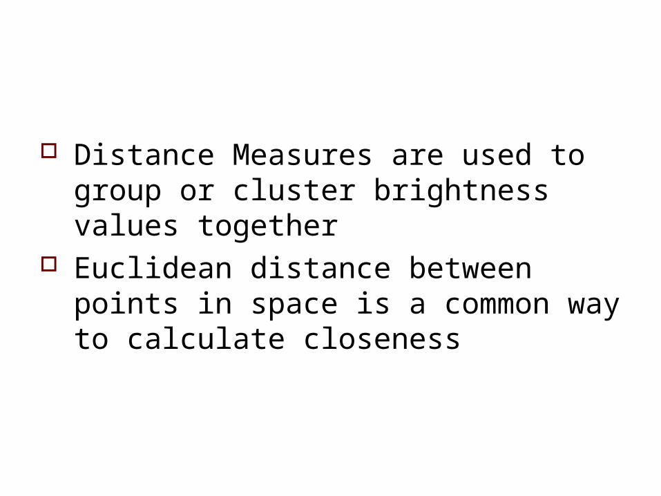
Distance Measures are used to group or cluster brightness values together

Euclidean distance between points in space is a common way to calculate closeness

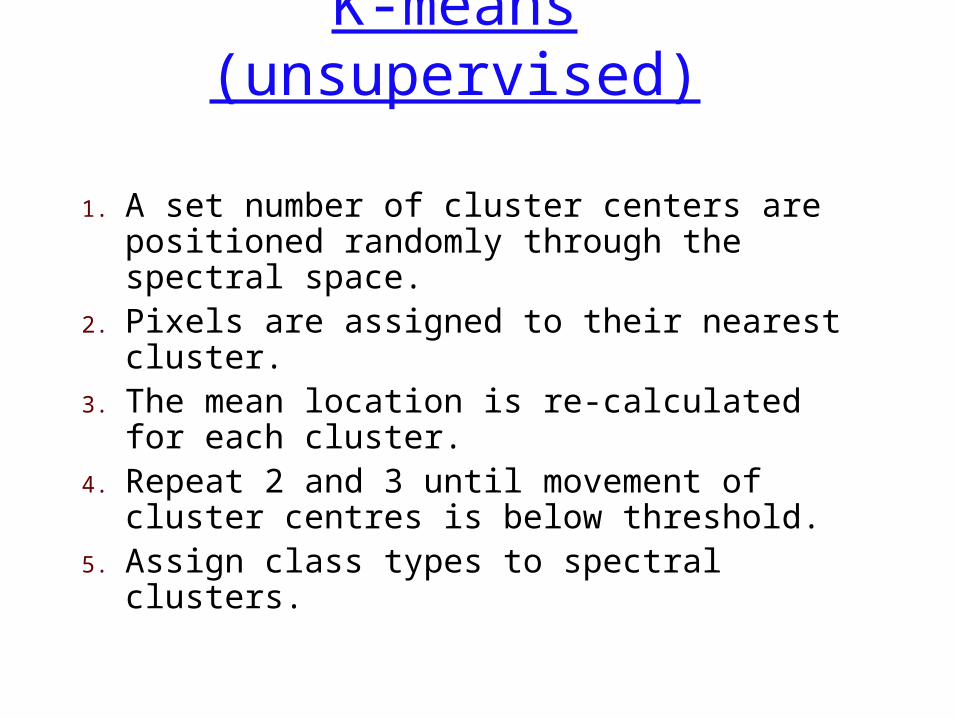
K-means (unsupervised)

1. A set number of cluster centers are positioned randomly through the spectral space.

2. Pixels are assigned to their nearest cluster.3. The mean location is re-calculated for each

cluster.4. Repeat 2 and 3 until movement of cluster

centres is below threshold.5. Assign class types to spectral clusters.

Example k-means

Band 1

Ban

d 2

Band 1

Ban

d 2

Band 1

Ban

d 2

1. First iteration. The cluster centers are set at random. Pixels will be assigned to the nearest center.

2. Second iteration. The centers move to the mean-center of all pixels in this cluster.

3. N-th iteration. The centers have stabilized.

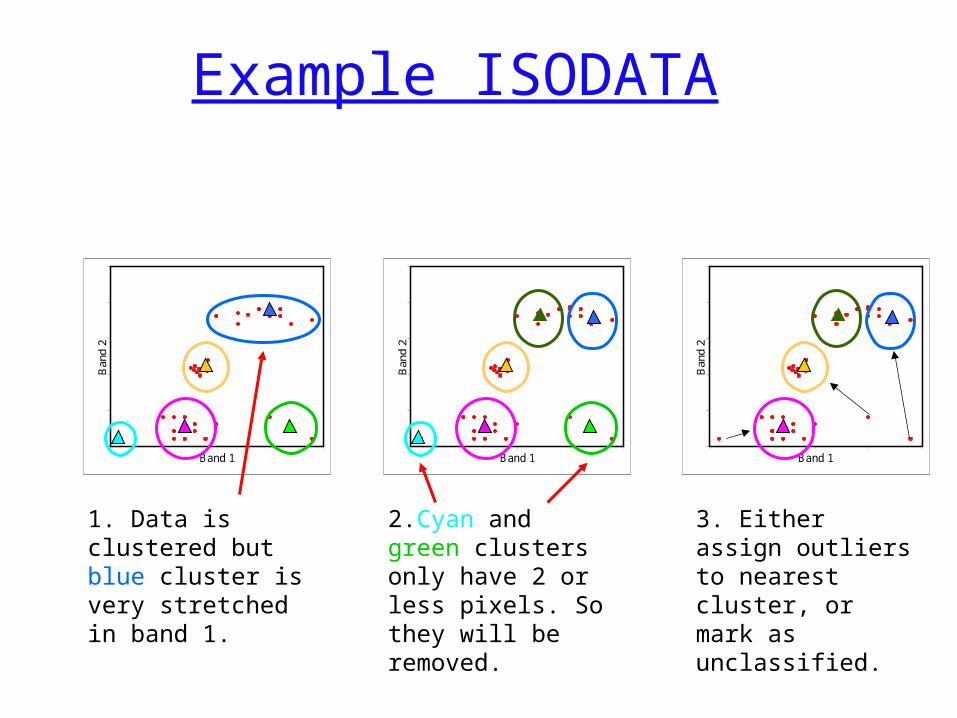
Example ISODATA

Band 1

Ban

d 2

1. Data is clustered but blue cluster is very stretched in band 1.

2.Cyan and green clusters only have 2 or less pixels. So they will be removed.

Band 1

Ban

d 2

Band 1

Ban

d 2

3. Either assign outliers to nearest cluster, or mark as unclassified.

ISODATA: Initial Cluster Values (properties)

number of classes maximum iterationspixel change threshold (0 - 100%) (The change

threshold is used to end the iterative process when the number of pixels in each class changes by less than the threshold. The classification will end when either this threshold is met or the maximum number of iterations has been reached)

initializing from statistics (Erdas) or from input (ENVI) (the initial values to put in for ENVI are minimum # pixel in class, maximum class stdv, minimum class distance, maximum # merge pairs)

Maximum Class Stdv (in pixel value). If the stdv of a class is larger than this threshold then the class is split into two classes.Minimum class distance (in pixel value) between class means. If the distance between two class means is less than the minimum value entered, then ENVI merges the classes.

Optional Maximum stdev from mean (1 to 3σ) and maximum distance error (in pixel value). If any of these two setup, the some pixels might not be classified.

5-10 classes, 8 iterations, 5 for change threshold, (MinP 5, MaxSD 1, MinD 5, MMP 2)

1-5 classes, 11 iterations, 5 for change threshold, (MinP 5, MaxSD 1, MinD 5, MMP 2)

5 classes

10 classes

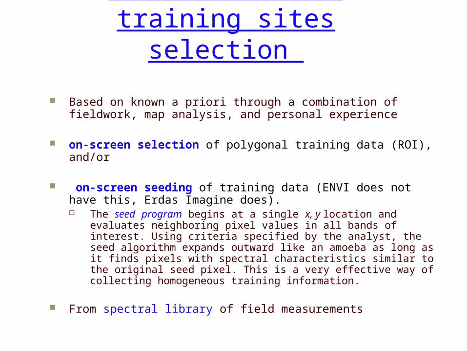
2. Supervised classification:training sites selection

Based on known a priori through a combination of fieldwork, map analysis, and personal experience

on-screen selection of polygonal training data (ROI), and/or

on-screen seeding of training data (ENVI does not have this, Erdas Imagine does). The seed program begins at a single x, y location and evaluates

neighboring pixel values in all bands of interest. Using criteria specified by the analyst, the seed algorithm expands outward like an amoeba as long as it finds pixels with spectral characteristics similar to the original seed pixel. This is a very effective way of collecting homogeneous training information.

From spectral library of field measurements

Advantages Analyst has control over the selected classes

tailored to the purpose Has specific classes of known identity Does not have to match spectral categories on the

final map with informational categories of interest

Can detect serious errors in classification if training areas are missclassified

Disadvantages Analyst imposes a classification (may not be

natural) Training data are usually tied to informational

categories and not spectral properties Remember diversity

Training data selected may not be representative Selection of training data may be time consuming

and expensive May not be able to recognize special or unique

categories because they are not known or small

Statistic extraction of each training site

kji

ji

ji

ji

c

BV

BV

BV

BV

X

,,

3,,

2,,

1,,

.

.

kji

ji

ji

ji

c

BV

BV

BV

BV

X

,,

3,,

2,,

1,,

.

.

where BVi,j,k is the brightness value for the i,jth pixel in band k. µck represents the mean value of all pixels obtained for class c in band k. Covckl is the covariance of class c between bands l through k.

where BVi,j,k is the brightness value for the i,jth pixel in band k. µck represents the mean value of all pixels obtained for class c in band k. Covckl is the covariance of class c between bands l through k.

Each pixel in each training site associated with a particular class (c) is represented by a measurement vector, Xc; Average of all pixels in a training site called mean vector, Mc; a covariance matrix of Vc.

Each pixel in each training site associated with a particular class (c) is represented by a measurement vector, Xc; Average of all pixels in a training site called mean vector, Mc; a covariance matrix of Vc.

ck

c

c

c

cM

.

.3

2

1

ck

c

c

c

cM

.

.3

2

1

ckkckck

kccc

kccc

cV

cov...covcov

.

.

cov...covcov

cov...covcov

21

22221

11211

ckkckck

kccc

kccc

cV

cov...covcov

.

.

cov...covcov

cov...covcov

21

22221

11211

SelectingSelectingROIsROIs

Alfalfa

Cotton

Grass

Fallow

Spectra of ROIs from ETM+ image

Spectra from library

Resampled to matchTM/ETM+, 6 bands

Supervised classification methods

Various supervised classification algorithms may be used to assign an unknown pixel to one of m possible classes. The choice of a particular classifier or decision rule depends on the nature of the input data and the desired output. Parametric classification algorithms assumes that the observed measurement vectors Xc obtained for each class in each spectral band during the training phase of the supervised classification are Gaussian; that is, they are normally distributed. Nonparametric classification algorithms make no such assumption.

Several widely adopted nonparametric classification algorithms include: one-dimensional density slicing parallepiped, minimum distance, nearest-neighbor, and neural network and expert system analysis.

The most widely adopted parametric classification algorithms is the: maximum likelihood.

Hyperspectral classification methods Binary Encoding Spectral Angle Mapper Matched Filtering Spectral Feature Fitting Linear Spectral Unmixing

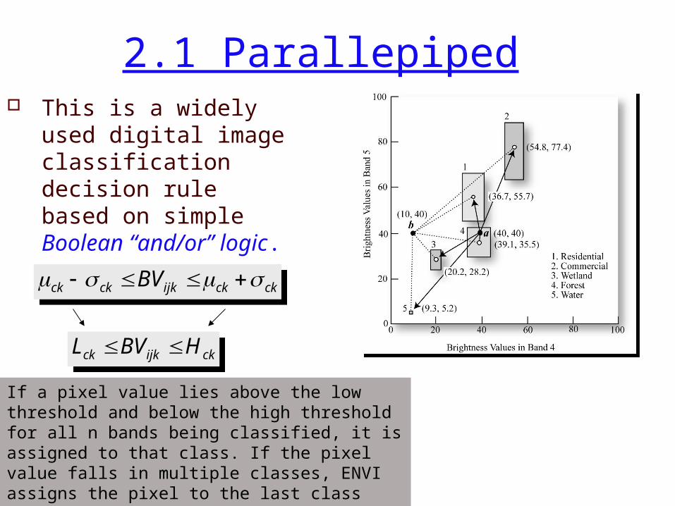
2.1 Parallepiped This is a widely used

digital image classification decision rule based on simple Boolean “and/or” logic.

ckckijkckck BV ckckijkckck BV

ckijkck HBVL ckijkck HBVL

If a pixel value lies above the low threshold and below the high threshold for all n bands being classified, it is assigned to that class. If the pixel value falls in multiple classes, ENVI assigns the pixel to the last class matched. Areas that do not fall within any of the parallelepipeds are designated as unclassified. In ENVI, you can use 1-3

This method is a computationally efficient method. But an unknown pixel might meet the criteria of more than one class and is always assigned to the first class for which it meets all criteria. The Minimum Distance to Means can assign any pixel to just one class.

Parallelepiped example

Training classes plotted in spectral space. In this example using 2 bands.

Parallelepiped example continued

•Each class type defines a spectral box

•Note that some boxes overlap even though the classes are spatially separable.

•This is due to band correlation in some classes.

•Can be overcome by customising boxes.

1 means 1 stdev from mean, 2 means 2 stdev from mean, 3 means 3 stdev from mean;Use 1, you will classify the closest pixels to the classUse 3, you will include some not so closest pixels to the class

2.2 Minimum distance

22clijlckijk BVBVDist 22

clijlckijk BVBVDist

22clijlckijk BVBVDist 22

clijlckijk BVBVDist

The distance used in a minimum distance to means classification algorithm can take two forms: the Euclidean distance based on the Pythagorean theorem and the “round the block” distance. The Euclidean distance is more computationally intensive, but it is more frequently used

The distance used in a minimum distance to means classification algorithm can take two forms: the Euclidean distance based on the Pythagorean theorem and the “round the block” distance. The Euclidean distance is more computationally intensive, but it is more frequently used

6.45.35401.3940 22 Dist 6.45.35401.3940 22 Dist

22clijlckijk BVBVDist 22

clijlckijk BVBVDist

e.g. the distance of point a to class forest is

All pixels are classified to the nearest class unless a standard deviation or distance threshold is specified, in which case some pixels may be unclassified if they do not meet the selected criteria.

If either Max stdev or Max distance error is not set, all pixels will be classified.If the Max stdev from mean is set at 2 (stdev), then the pixels with values outside the mean ± 2σ will not be classified. If the Max distance error is set at 4.2 (pixel value), then the pixels with distance larger than 4.2 will not be classified.

2.3 Maximum likelihood

Instead based on training class multispectral distance measurements, the maximum likelihood decision rule is based on probability.

The maximum likelihood procedure assumes that each training class in each band are normally distributed (Gaussian). Training data with bi- or n-modal histograms in a single band are not ideal. In such cases the individual modes probably represent unique classes that should be trained upon individually and labeled as separate training classes.

the probability of a pixel belonging to each of a predefined set of m classes is calculated based on a normal probability density function, and the pixel is then assigned to the class for which the probability is the highest. probability

The estimated The estimated probability density functionprobability density function for class for class wwii (e.g., forest) is computed using (e.g., forest) is computed using

the equation:the equation:

where where expexp [ ][ ] is is ee (the base of the natural logarithms) raised to the computed power, (the base of the natural logarithms) raised to the computed power, xx is one of the brightness values on the is one of the brightness values on the xx-axis, is the estimated mean of all the values -axis, is the estimated mean of all the values in the forest training class, and is the estimated variance of all the measurements in in the forest training class, and is the estimated variance of all the measurements in this class. this class. Therefore, we need to store only the mean and variance of each training Therefore, we need to store only the mean and variance of each training class (e.g., forest) to compute the probability function associated with any of the class (e.g., forest) to compute the probability function associated with any of the individual brightness values in it.individual brightness values in it.

The estimated The estimated probability density functionprobability density function for class for class wwii (e.g., forest) is computed using (e.g., forest) is computed using

the equation:the equation:

where where expexp [ ][ ] is is ee (the base of the natural logarithms) raised to the computed power, (the base of the natural logarithms) raised to the computed power, xx is one of the brightness values on the is one of the brightness values on the xx-axis, is the estimated mean of all the values -axis, is the estimated mean of all the values in the forest training class, and is the estimated variance of all the measurements in in the forest training class, and is the estimated variance of all the measurements in this class. this class. Therefore, we need to store only the mean and variance of each training Therefore, we need to store only the mean and variance of each training class (e.g., forest) to compute the probability function associated with any of the class (e.g., forest) to compute the probability function associated with any of the individual brightness values in it.individual brightness values in it.

2

2

2

1 ˆ

ˆ

2

1exp

ˆ2

1|ˆ

i

i

i

i

xwxp

2

2

2

1 ˆ

ˆ

2

1exp

ˆ2

1|ˆ

i

i

i

i

xwxp

ii2ˆ i

2ˆ i

For multiple bands of remote sensor data for the classes of interest, we compute an n-dimensional multivariate normal density function using:

where is the determinant of the covariance matrix, is the inverse of the covariance matrix, and is the transpose of the vector . The mean vectors (Mi) and covariance matrix (Vi) for each class are estimated from the training data.

For multiple bands of remote sensor data for the classes of interest, we compute an n-dimensional multivariate normal density function using:

where is the determinant of the covariance matrix, is the inverse of the covariance matrix, and is the transpose of the vector . The mean vectors (Mi) and covariance matrix (Vi) for each class are estimated from the training data.

TiMX TiMX || iV|| iV 1

iV1

iV

iMX iMX

iiT

i

i

ni MXVMX

V

wXp 1

2

1

22

1exp

||2

1|

iiT

i

i

ni MXVMX

V

wXp 1

2

1

22

1exp

||2

1|

Without Prior Probability InformationWithout Prior Probability Information:: Decide unknown measurement vector Decide unknown measurement vector XX is is in class in class ii if, and only if, if, and only if,ppii >> p pjj

for allfor all ii andand j j out of 1, 2, ...out of 1, 2, ... mm possible possible classes andclasses and

iiT

iiei MXVMXVp 1

2

1||log

2

1

iiT

iiei MXVMXVp 1

2

1||log

2

1

Unless you select a probability threshold (0-1), all pixels are classified. Each pixel is assigned to the class that has the highest probability

The assign the measurement vector X of an unknown pixel to a class, the maximum likelihood decision rule computers the value pi for each class. Then it assigns the pixel to the class that has the largest value

Probability threshold from [0, 1]. 0 means zero probability of similarity, 1 means 100% probability of similarity.

2.4 Mahalanobis Distance

M-distance is similar to the Euclidian distance

iiT

i MXVMXDist 1 iiT

i MXVMXDist 1

It is similar to the Maximum Likelihood classification but assumes all class covariances are equal and therefore is a faster method. All pixels are classified to the closest ROI class unless you specify a distance threshold, in which case some pixels may be unclassified if they do not meet the threshold (in DN number)

2.5 Spectral Angle Mapper

2.6 Spectral Feature Fitting

compare the fit of image reflectance spectra to selected reference reflectance spectra using a least-squares techniqueleast-squares technique. SFF is an absorption-feature-based methodology. Both reflectance spectra should be continuum removed.

A scale image is output for each reference spectrum and is a measure of absorption feature depth which is related to material abundance. The image and reference spectra are compared at each selected wavelength in a least-squares sense and the root mean square (rms) error is determined for each reference spectrum.

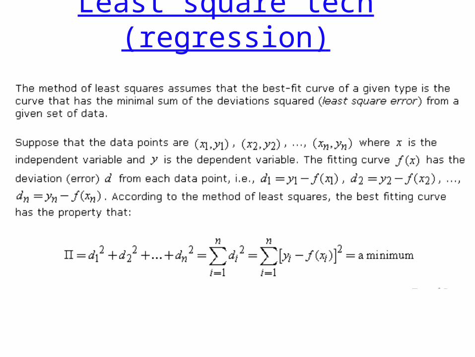
Least square tech (regression)

A continuum is a mathematical function used to isolate a particular absorption feature for analysis

Source: http://popo.jpl.nasa .gov/html/data.html

Supervisedclassificationmethod:

Spectral FeatureFitting