Chung R. Song, Ph.D., A.E.Associate ProfessorDepartment of Civil EngineeringUniversity of Nebraska-Lincoln

“This report was funded in part through grant[s] from the Federal Highway Administration [and Federal Transit Administration], U.S. Department of Transportation. The views and opinions of the authors [or agency] expressed herein do not necessarily state or reflect those of the U.S. Department of Transportation.”

Nebraska Transportation Center262 Prem S. Paul Research Center at Whittier School2200 Vine StreetLincoln, NE 68583-0851(402) 472-0141

Binyam M. BekeleGraduate Research Assistant

Brian SawyerUndergraduate Research Assistant

Piezocone Penetration Testing Device

2018

Nebraska Transportation Center

Final Report26-1121-4038-001Report M063

PIEZOCONE PENETRATION TESTING DEVICE

Submitted By

Chung R. Song, Ph.D., A.E. Principal Investigator

Binyam M. Bekele

Graduate Research Assistant

Brian Sawyer Undergraduate Research Assistant

and

University of Nebraska-Lincoln

Submitted to

Nebraska Department of Transportation

1500 Nebraska Highway 2

Lincoln, Nebraska 68502

Project Duration (7/1/2016 to 12/30/2017)

February 2, 2018

ii

TECHNICAL REPORT DOCUMENTATION PAGE

1. Report No.

M063 2. Government Accession No. 3. Recipient’s Catalog No.

4. Title and Subtitle Piezocone Penetration Testing Device

5. Report Date January 3, 2017 6. Performing Organization Code:

7. Author(s) Chung R. Song, Binyam M. Bekele and Brian Sawyer

8. Performing Organization Report No. 26-1121-4038-001

9. Performing Organization Name and Address University of Nebraska-Lincoln, Department of Civil Engineering 262 Prem Paul Research Center at Whittier School 2200 Vine St, Lincoln, NE 68503

10. Work Unit No. 11. Contract or Grant No.

12. Sponsoring Agency Name and Address Nebraska Department of Transportation (NDOT) 1500 Nebraska Highway 2 Lincoln, NE 68502

13. Type of Report and Period 14. Sponsoring Agency Code

15. Supplementary Notes 16. Abstract Hydraulic characteristics of soils can be estimated from piezocone penetration test (called PCPT hereinafter) by performing dissipation test or on-the-fly using advanced analytical techniques. This research report presents a method for fast estimation of hydraulic conductivity of overconsolidated soils based on the piezocone penetration test. The method relies on an existing relationship developed for the determination of hydraulic conductivity of normally consolidated soils on-the-fly. The present research revises this relationship so that it can be applied for overconsolidated soils by incorporating a proper correction equation. The revised relationship provides a pore pressure representing the hydraulic conductivity of a hypothetical “equivalent normally consolidated soil”. The revised relationship was developed with piezocone indices (Qt, Fr, and Bq) based on well documented laboratory test and PCPT data. In this regard, PCPT data from Nebraska Department of Transportation (NDOT) was used as a primary data base to determine the correction equation. Then, the proposed revised relationship was verified for other sites in the USA, Canada, and South Korea. This study showed that the proposed method provides a reasonably good prediction of hydraulic conductivity of overconsolidated soils. In addition, the method also accurately predicted the hydraulic conductivity of normally consolidated soils.

17. Key Words

Hydraulic conductivity; Overconsolidated soil; PCPT; Piezocone indices

18. Distribution Statement

19. Security Classification (of this report) Unclassified

20. Security Classification (of this page) Unclassified

21. No. of Pages 88

22. Price

iii

TABLE OF CONTENTS

LIST OF TABLES .............................................................................................................. v LIST OF FIGURES ........................................................................................................... vi ACKNOWLEDGMENTS ............................................................................................... viii DISCLAIMER ................................................................................................................... ix ABSTRACT ........................................................................................................................ x

1 INTRODUCTION .............................................................................................................. 1 1.1 Background ............................................................................................................. 1 1.2 General Insight of the New Technique ................................................................... 2 1.3 Objectives of the Project ......................................................................................... 3

2 LITERATURE REVIEW ................................................................................................... 4 2.1 Background ............................................................................................................. 4 2.2 Pore Pressure Response in PCPT ............................................................................ 4 2.3 Evaluation of Hydraulic Conductivity from PCPT ................................................. 6

2.3.1 Prediction of Hydraulic Properties from Dissipation Curves ...................... 7 2.3.2 Prediction of Hydraulic Properties from On-The-Fly PCPT .................... 13

2.4 Conclusion ............................................................................................................ 20

3 PRELIMINARY EVALUATION OF HYDRAULIC CONDUCTIVITY BASED ON LABORATORY TEST AND PCPT ........................................................................................... 22

3.1 Background ........................................................................................................... 22 3.2 Data Collection and Organization ......................................................................... 23 3.3 Estimation of Hydraulic Conductivity from Laboratory Test Results .................. 23 3.4 Estimation of Hydraulic Conductivity Based on PCPT ........................................ 26

3.4.1 Strength and Compressibility Parameters (M and κ) ................................ 28 3.4.2 Adjustment Factors to Compensate for Overconsolidation Effect ........... 29

3.5 Sample Hydraulic Conductivity Profiles with Depth ........................................... 32

4 ADDITIONAL EVALUATIONS ON THE CORRELATION AND CASE STUDIES . 34 4.1 Introduction ........................................................................................................... 34 4.2 Evaluation of Data Points with negative and Positive Pore Pressure Ratio (Bq) .. 35

4.2.1 Qualitative Evaluation ............................................................................... 35 4.2.2 Quantitative Evaluation ........................................................................................ 38 4.3 Evaluation of the Correlation for other Sites ........................................................ 41

4.3.1 Yangsan Mulgeum, Korea (Dong A Geology 1997) ................................ 41 4.3.2 Frazer River, Canada (Crawford and Campanella 1991) .......................... 42 4.3.3 Cheongna (Section 1), Incheon, Korea (Kaya Engineering Co. 2007) ..... 44

iv

4.3.4 SR 49, Indiana, USA ................................................................................. 45 4.4 Hydraulic Conductivity Determination Program .................................................. 46

4.4.1 Program Development (Version 1) ........................................................... 47 4.4.2 User Form .................................................................................................. 47 4.4.3 Future Capabilities .................................................................................... 50

5 IMPROVED CORRELATION BETWEEN ADJUSTMENT FACTORS AND SBTn PARAMETERS ........................................................................................................................... 53

5.1 General .................................................................................................................. 53 5.2 Previously Established Relationship ..................................................................... 54 5.3 Improved Interpretation of Non-Dimensional Parameter ..................................... 55 5.4 Results and Interpretation ..................................................................................... 56 5.5 Verification with other Test data .......................................................................... 61

5.5.1 Yangsan Mulgeum, Korea (Dong A Geology 1997) ................................ 61 5.5.2 Frazer River, Canada (Crawford and Campanella 1991) .......................... 62 5.5.3 Cheongna (Section 1), Incheon, Korea (Kaya Engineering Co. 2007) ..... 64 5.5.4 SR 49, Indiana, USA (Kim 2005) ............................................................. 65

6 PCPT DATA INTERPRETER USER GUIDE (VERSION 2)......................................... 67

7 CONCLUSION ................................................................................................................. 74 References ......................................................................................................................... 75 Appendix A ....................................................................................................................... 77 Appendix B ....................................................................................................................... 79 Appendix C ....................................................................................................................... 83 Appendix D ....................................................................................................................... 85

v

LIST OF TABLES

Table 3.1 Computation of mv from the given consolidation test results ...................................... 24 Table 3.2. Hydraulic conductivity based on laboratory test results for project 2-6(119) RO-1 ... 26 Table 3.3. Hydraulic conductivity based on PCPT for project 2-6(119) RO-1 ............................ 28 Table 3.4. Computation of adjustment factors and SBTn parameters .......................................... 30 Table A.1 Summary of project identifications and amount of data .............................................. 77 Table B.1 Hydraulic conductivity estimated based on laboratory test results .............................. 79 Table C.1 Relationship between adjustment factors and N .......................................................... 83 Table D.1 Sample hydraulic conductivity computation based on PCPT ...................................... 85

vi

LIST OF FIGURES

Fig. 2.1. Pore pressure dissipation response in normally consolidated and lightly overconsolidated soils ................................................................................................................................................. 5 Fig. 2.2. Pore pressure dissipation response in overconsolidated soils .......................................... 5 Fig. 2.3. Conceptual pore pressure response for soil element during piezocone penetration ......... 6 Fig. 2.4. Dissipation curve prediction from spherical cavity .......................................................... 8 Fig. 2.5. Dissipation curve for 18o (uncoupled analysis) ................................................................ 9 Fig. 2.6. Effect of coupling on the dissipation curves for 18o cone (Isotropic Analysis) ............ 10 Fig. 2.7. Excess pore pressure dissipation curves at different locations for a soil with 𝑰𝑰𝑰𝑰=100 .. 11 Fig. 2.8. Excess pore pressure dissipation for the modified time factor, T* ................................ 12 Fig. 2.9. The effects of penetration speed ..................................................................................... 15 Fig. 2.10. Comparison of actual test data indicated by numbers from 1 to 13 with predicted results of dimensionless pore pressure and dimensionless hydraulic conductivity (M=1.2 and H=1.16) 16 Fig. 3.1. Stain versus change in effective stress .......................................................................... 25 Fig. 3.2 Excess pore pressure Vs hydraulic conductivity ............................................................. 27 Fig. 3.3. Correlation between adjustment factors and non-dimensional factor N ........................ 31 Fig. 3.4. Predicted hydraulic conductivity profiles with depth based on PCPT ........................... 33 Fig. 4.1. Normalized soil behavior type (SBTn) chart (after Robertson 2010) ............................ 35 Fig. 4.2. Dissipation of pore pressure for contractive and dilative soils (adapted from Burns and Mayne 1998) ................................................................................................................................. 36 Fig. 4.3. Hypothetical dissipation of pore pressure in heavily overconsolidated soils ................. 37 Fig. 4.4. Classification of soils in Nebraska using SBTn chart ..................................................... 39 Fig. 4.5. C vs modified N for negative and positive Bq data points (a) without reflection (semi log scale) (b) by reflection about N* axis (full log scale) ................................................................... 39 Fig. 4.6. C vs N* incorporating both negative and positive Bq .................................................... 40 Fig. 4.7. (a) SBTn classification and range of hydraulic conductivity (b) Estimated hydraulic property profile with depth for Yangsan, korea ............................................................................ 41 Fig. 4.8. (a) SBTn classification and range of hydraulic conductivity (b) Estimated hydraulic property profile with depth for Frazer River................................................................................. 43 Fig. 4.9 (a) SBTn classification and range of hydraulic conductivity (b) Estimated hydraulic property profile with depth for Frazer River................................................................................. 45 Fig. 4.10 (a) SBTn classification and range of hydraulic conductivity (b) Estimated hydraulic property profile with depth for Frazer River................................................................................. 46 Fig. 4.11. VBA user form ............................................................................................................. 48 Fig. 4.12. User selection of PCPT................................................................................................. 49 Fig. 4.13. Background ................................................................................................................... 50 Fig. 4.14. Modified image of user form to display correct plot .................................................... 51 Fig. 5.1. C vs N* incorporating both negative and positive Bq .................................................... 54 Fig. 5.2. Correlation between C and N (a) based on sleeve friction (b) based on cone resistance 57 Fig. 5.3 Hydraulic conductivity estimated based on Song and Pulijala........................................ 60

vii

Fig. 5.4. (a) SBTn classification (b) Estimated hydraulic property profile with depth for Yangsan Mulgeum, korea ............................................................................................................................ 62 Fig. 5.5.(a) SBTn classification (b) Estimated hydraulic property profile with depth for Frazer River ............................................................................................................................................. 63 Fig. 5.6. (a) SBTn classification (b) Estimated hydraulic property profile with depth for Cheongna, Incheon, Korea .............................................................................................................................. 65 Fig. 5.7. (a) SBTn classification (b) Estimated hydraulic property profile with depth for SR 49, Indiana, USA................................................................................................................................. 66 Fig. 6.1 Operating scree without macros enabled ......................................................................... 68 Fig. 6.2 User form on startup ........................................................................................................ 69 Fig. 6.3. File explorer to select PCPT data ................................................................................... 70 Fig. 6.4 PCPT “.CSV” output columns A-D ................................................................................ 71 Fig. 6.5 Plotted hydraulic conductivity profile on user form ........................................................ 72 Fig. 6.6 Excel sheet resulting from “Export Chart” button........................................................... 73 Fig. 6.7 Built in user manual ......................................................................................................... 73

viii

ACKNOWLEDGMENTS

The authors would like to thank Nebraska Department of Transportation (NDOT) for the financial

support needed to complete this research. Also, NDOT Technical Advisory Committee (TAC) for

their technical support, discussion and comments.

ix

DISCLAIMER

The contents of this report reflect the views of the authors, who are responsible for the facts and

the accuracy of the information presented herein. This document is disseminated under the

sponsorship of the U.S. Department of Transportation’s University Transportations Centers

Program, in the interest of information exchange. The U.S. Government assumes no liability for

the contents or use thereof.

x

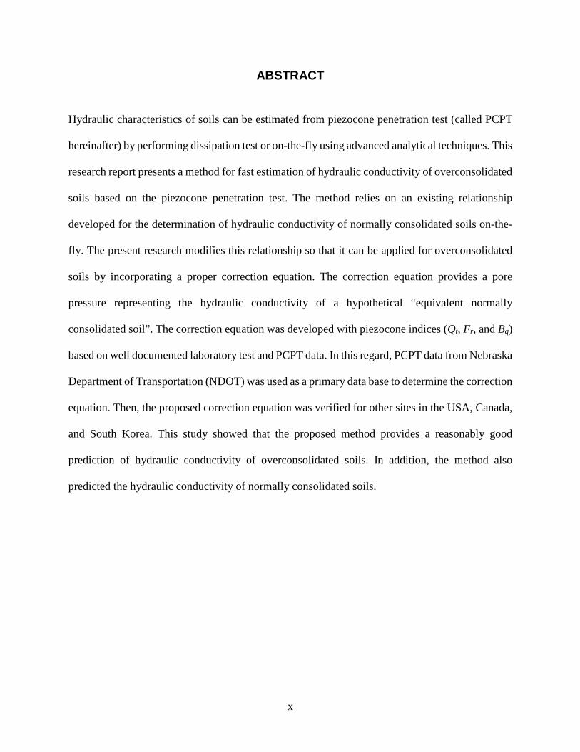
ABSTRACT

Hydraulic characteristics of soils can be estimated from piezocone penetration test (called PCPT

hereinafter) by performing dissipation test or on-the-fly using advanced analytical techniques. This

research report presents a method for fast estimation of hydraulic conductivity of overconsolidated

soils based on the piezocone penetration test. The method relies on an existing relationship

developed for the determination of hydraulic conductivity of normally consolidated soils on-the-

fly. The present research modifies this relationship so that it can be applied for overconsolidated

soils by incorporating a proper correction equation. The correction equation provides a pore

pressure representing the hydraulic conductivity of a hypothetical “equivalent normally

consolidated soil”. The correction equation was developed with piezocone indices (Qt, Fr, and Bq)

based on well documented laboratory test and PCPT data. In this regard, PCPT data from Nebraska

Department of Transportation (NDOT) was used as a primary data base to determine the correction

equation. Then, the proposed correction equation was verified for other sites in the USA, Canada,

and South Korea. This study showed that the proposed method provides a reasonably good

prediction of hydraulic conductivity of overconsolidated soils. In addition, the method also

predicted the hydraulic conductivity of normally consolidated soils.

1

1 INTRODUCTION

1.1 Background

The piezocone penetration testing device is known as one of the two more reliable geotechnical

testing devices (Lunne et al. 1997), and NDOT has one portable unit which is actively deployed

on their existing drill rigs. The built-in piezometer in the piezocone measures the pore pressure

response during penetration and used to profile soil layering systems.

For saturated soils, this piezometer is also used to conduct dissipation tests to obtain hydraulic

conductivity or coefficient of consolidation. Dissipation tests usually takes four to eight hours,

which considerably lowers the testing efficiency (speed) of this device. (Usually it takes one to

two hours for one piezocone test without dissipation test while it takes one whole day with a

dissipation test.)

Recently a technique was developed by Song and Pulijala (2010) to estimate the hydraulic

conductivity or coefficient of consolidation without resorting to the dissipation tests. Song and

Pulijala’s 2010 method is essentially an advanced analytical technique that doesn’t need any

mechanical modification of the existing piezocone system. Infusing Song and Pulijala (2010) to

the current piezocone system of NDOT will provide real time estimation of hydraulic conductivity

information. Once this technique is incorporated into the current NDOT’s piezocone system, the

efficiency of the piezocone penetration testing device will be significantly improved with no or

little additional cost.

2

1.2 General Insight of the New Technique

Several methods to evaluate hydraulic properties using the piezocone penetrometer have recently

been developed. Rust et al. (1995) estimated the coefficient of consolidation from pore pressure

dissipation data obtained during the arresting time for the drive rod connection (at every one meter

interval). Manassero (1994) proposed an empirical approach to estimate the hydraulic conductivity

of slurry walls. Song et al. (1999) estimated the hydraulic conductivity of soils from the pore

pressure difference between u2 and u3 measured PCPT. It is noted that u2 is measured pore pressure

at the cone tip shoulder. u3 is measured pore pressure at the cone shaft that is approximately 14 cm

apart from u2 location. When one compares pore pressure at the cone shaft that is approximately

14 cm time difference between the two measurements, one can see that the pore pressure at u3 is

usually different from that at u2. The difference shall be due to the dissipation of excess pore

pressure in seven seconds with reference penetration speed 2 cm/s of piezocone penetrometer. By

analyzing this pore pressure dissipation, Song et al. (1999) were able to estimate the hydraulic

conductivity of soils. Song and Pulijala (2010) further developed a technique so that the

computation time is decreased and “on-the-fly” computation of the hydraulic conductivity of soils

from piezocone penetration tests can be done.

Song and Pulijala’s technique is based on the notion of simultaneous generation and dissipation of

excess pore pressure at a given point. Pore pressure will be generated due to the imposed stress

by the penetration and redistribution of in-situ stress condition. However, the notion of

simultaneous generation and dissipation states that this generated pore pressure at a given point

also contains dissipation information for previously generated pore pressure before the

penetrometer reaches to that point.

3

Analytical solutions to solve the simultaneous generation and dissipation of excess pore pressure

are available (Elsworth and Lee 200, Voyiadjis and Song 2003), but the computation costs are

quite high due to sophisticated numerical techniques. The parametric studies and semi-empirical

equations proposed by Song and Pulijala (2010) provide a simpler and faster way of determining

the hydraulic conductivity from PCPT.

1.3 Objectives of the Project

The main objective of the project is to estimate hydraulic conductivity of soils on real time basis

using NDOT’s piezocone penetration test device. The following detailed objectives were planned:

(a) Real time determination of hydraulic conductivity of soils based on Song and Pulijala’s

2010 equation.

(b) Find correlation between measured excess pore pressure and hydraulic conductivity of

Nebraska’s Soils (overconsolidated soils).

(c) Conduct experiments in a well-controlled environment to confirm the correlations obtained

in (b).

(d) Implement Correlations in NDOT’s piezocone penetration test (PCPT) device (Data

Logger/Computer) so that the hydraulic conductivity profile is obtained ‘on-the-fly’ with

other outputs such as tip resistance, side friction, pore pressure and soil classification.

4

2 LITERATURE REVIEW

2.1 Background

The piezocone sounding device is the most reliable, rapid, and cost-effective testing device utilized

to determine the type, stratification, mechanical and transport behavior of soils (Lunne et al.,

1997). Today, due to their cost effectiveness and mobility, they are widely used in geotechnical

site investigation, quality control of construction, ground improvement and in deep foundations.

In particular, the hydraulic characteristics of soils can be estimated from piezocone penetration

test (called PCPT hereinafter) by performing dissipation test or on-the-fly using advanced

analytical techniques. The hydraulic characteristics of soils predominantly controlled by the

coefficient of consolidation and the hydraulic conductivity of soil solid matrix. In this chapter, a

review of available methods and underlying concepts is carried out regarding the evaluation of

hydraulic conductivity and coefficient of consolidation using dissipation and on-the-fly testing.

2.2 Pore Pressure Response in PCPT

Advancing the penetrometer into the soil continually exerts an axial force onto the soil elements

at different depths. For saturated soils, this vertical penetration from the tip of the penetrometer

induces excess pore water pressure. However, when the penetration is halted, dissipation of the

excess pore pressure generated will be initiated and it will continue to dissipate until it comes to

the initial hydrostatic condition. Based on the rate of dissipation of the excess pore pressure, the

magnitudes of hydraulic conductivity and coefficient of consolidation can be obtained.

A typical pore pressure dissipation response shows a continuous reduction of excess pore pressure

with time after arresting the penetrometer, which is like the response in oedometer tests as shown

5

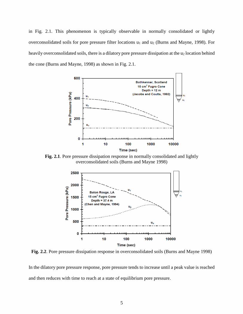
in Fig. 2.1. This phenomenon is typically observable in normally consolidated or lightly

overconsolidated soils for pore pressure filter locations u1 and u2 (Burns and Mayne, 1998). For

heavily overconsolidated soils, there is a dilatory pore pressure dissipation at the u2 location behind

the cone (Burns and Mayne, 1998) as shown in Fig. 2.1.

Fig. 2.1. Pore pressure dissipation response in normally consolidated and lightly overconsolidated soils (Burns and Mayne 1998)

Fig. 2.2. Pore pressure dissipation response in overconsolidated soils (Burns and Mayne 1998)

In the dilatory pore pressure response, pore pressure tends to increase until a peak value is reached

and then reduces with time to reach at a state of equilibrium pore pressure.

6

The pore pressure response for normally and lightly overconsolidated soils follows the solid line

in Fig. 2.3 for a soil element located along the centerline of the travel path of the piezocone

penetrometer as suggested by Voyiadjis and Song (2003). As the penetrometer approaches to the

soil element, the additional stress from the penetrometer will induce excess pore pressure, and this

pore pressure tends to increase until the moment the cone tip passes through the soil element. When

the penetrating cone stops at this point, there is an immediate drop in pore pressure. After this, one

may see a small increase in pore pressure due to the interaction between near field and far field.

(near field: radially close to the cone, far field: radially far from the cone).

Fig. 2.3. Conceptual pore pressure response for soil element during piezocone penetration (Voyiadjis and Song 2003)

2.3 Evaluation of Hydraulic Conductivity from PCPT

This section briefly summarizes the major advancements in theoretical interpretations of piezocone

penetration test based on dissipation curves and from on-the-fly methods.

7

The theoretical evaluation or interpretation of dissipation curves requires the parameter you are

looking for, the magnitude of that parameter, the range of applicability it has, the length of time

the dissipation is allowed, and the location that the pore pressure is measured; at the face, behind

the cone or on the shaft (Baligh and Levandoux 1986). Baligh and Levandoux (1986) also

discussed the difficulties in the theoretical evaluation of dissipation tests. These difficulties arise

from the uncertainty associated with initial excess pore pressure determination and due to the

complexity of a soil’s mechanical behavior (non-linearity, anisotropy, rate dependency and non-

homogeneity) caused by remolding due to penetration. Because of these complexities in theoretical

interpretation of dissipation tests, few theoretical approaches have been developed, with nearly no

developments before the 1980s.

In recent years, studies have concentrated on the evaluation of hydraulic parameters from PCPT

on-the-fly. These techniques provide a real-time estimation of both the coefficients of

consolidation and hydraulic conductivity continuously without resorting to dissipation tests. In

addition to this, on-the-fly evaluation of these parameters can considerably increase the efficiency

of PCPT through reduction of time consumed in performing dissipation tests. A brief discussion

about both techniques from various points of view is made in the subsequent sections.

2.3.1 Prediction of Hydraulic Properties from Dissipation Curves

Torstensson (1977) (cited in Burns and Mayne 1998) did the first theoretical interpretation of

dissipation test using cavity expansion theory for one-dimensional (radial) dissipation. In this

work, the soil was assumed to behave as an elastic-perfectly plastic material. The Terzaghi-

Rendulic uncoupled one-dimensional consolidation theory was used for the interpretation of the

coefficient of consolidation. The coefficient of consolidation is estimated by computing the time

8

factor for 50% degree of consolidation using the following expression and matching it with the

field dissipation data.

2

50

50ort

Tc = (2.1)

where T50 is the time factor at 50% degree of consolidation. The T50 is predicted from this theory

as a function of 𝐸𝐸𝑢𝑢/𝜏𝜏𝑓𝑓 and depends on the type of cavity (cylindrical or spherical). 𝐸𝐸𝑢𝑢 is equivalent

undrained elastic modulus and 𝜏𝜏𝑓𝑓 is the maximum undrained shear strength. The t50 is the measured

time at 50% of consolidation and 𝑟𝑟𝑜𝑜 is an equivalent cavity radius. Torstensson stated that his

method overestimated field values by a factor of approximately 2 from dissipation records, which

were used to verify the model in normally consolidated clay. A sample dissipation curve from

Torstensson (1977) is shown in Fig. 2.4.

Baligh and Levandoux (1986) did a comprehensive work for the prediction of dissipation tests that

Torstensson did in 1977. The study used a strain path method to estimate the initial pore pressure

for re-sedimented normally consolidated Boston blue clay (BBC) with rigidity index 𝐼𝐼𝑟𝑟 = 100

.

Fig. 2.4. Dissipation curve prediction from spherical cavity (Torstensson, 1977)

9

The rigidity index is defined as 𝐼𝐼𝑟𝑟 = 𝐺𝐺𝑆𝑆𝑢𝑢� , where 𝐺𝐺 is the shear modulus and 𝑆𝑆𝑢𝑢 is the undrained

shear strength of the soil. This method was different from the cavity expansion method used by

Torstensson (1977) and accounted for both vertical and horizontal (radial) dissipations. The basis

for this interpretation method was the fact that penetration test is a strain controlled test.

The study utilizes linear material behavior. The authors argued that linear analysis provides

valuable normalizations that can be applied to a wide range of soils. The work encompassed both

uncoupled (Terzaghi theory) and coupled analysis (Biot’s theory) of consolidation and the effect

of cone angle, and anisotropy on dissipation response using finite difference analysis technique.

Unlike Torstensson (1977), pore pressures were predicted at four different locations: At the cone

tip, on the cone face, behind the cone, and on the shaft. Fig. 2.5 shows a sample dissipation curve

predicted from this theory for an 18o cone and using uncoupled consolidation analysis. Fig. 2.6

shows the comparison between uncoupled and coupled consolidation analysis for the 18o cone.

Fig. 2.5. Dissipation curve for 18o (uncoupled analysis)

10

Fig. 2.6. Effect of coupling on the dissipation curves for 18o cone (Isotropic Analysis)

In addition, based on field measurements of BBC at different locations on the cone and on the

shaft behind it, predicted values showed excellent agreement for both the 18° and 60° cones despite

the approximate nature of the strain path method. From this study, the following important points

were concluded:

a) A tenfold decrease in vertical coefficient of consolidation has a minor effect on the

dissipation rates. Therefore, dissipation is essentially controlled by the horizontal

coefficient of consolidation, as shown in Fig. 2.6.

b) Dissipation around the blunt cones (60o) are less sensitive to the filter location on the

face of the cone and less susceptible to computational errors.

c) For the 18° cone, the effect of coupling the total stresses with the pore pressures has a

minor effect on the dissipation rates after 20% consolidation, except at the cone tip, as

shown in Fig. 2.6.

11

Houlsby and Teh (1988) extended the work of Baligh and Levandoux (1986) by incorporating

large strain finite element technique besides the strain path method. This technique fulfills force

equilibrium, which the strain path method failed to do. The soil penetrated by the cone was

assumed to be an elastic-perfectly plastic material (obeys Von-Mises failure criterion), which was

different from the material model used in Baligh and Levadoux (1986). Unlike the work of Baligh

and Levandoux (1986), this study considered only uncoupled consolidation analysis. The pore

pressure dissipations were estimated at different filter locations, as was done by Baligh and

Levandoux (1986). A sample dissipation curve is shown in Fig. 2.7 for 𝐼𝐼𝑟𝑟=100.

The study conducted by Houlsby and Teh (1988) noted that due to the variation of 𝐼𝐼𝑟𝑟 from soil to

soil, the dissipation curves are not unique at a given filter location. The authors ultimately came

up with a new method to merge a family of dissipation curves into a unified curve by modifying

the time factor from T to T*. The modified time factor is obtained from the following expression:

r

h

IRtcT

2* = (2.2)

Fig. 2.7. Excess pore pressure dissipation curves at different locations for a soil with 𝑰𝑰𝑰𝑰=100

12

where ch is the horizontal coefficient of consolidation, R is the radius of the cone and 𝐼𝐼𝑟𝑟 is the

rigidity index. Fig. 2.8 shows the unified dissipation curves at the filter located behind the cone

for different 𝐼𝐼𝑟𝑟 values ranging from 50 to 500.

Fig. 2.8. Excess pore pressure dissipation for the modified time factor, T*

As a conclusion, the study stressed the importance of rigidity index to rationally interpret

dissipation curves. The authors also believed that a unique interpretation of dissipation curves is

achieved only if the time factor accounts for the effect of soil stiffness. Moreover, as Baligh and

Levandoux (1986) concluded, this study also concluded that the dissipation rate is strongly

controlled by the horizontal coefficient of consolidation.

Elsworth (1993) proposed a theoretical method of dissipation test interpretation which was quite

different than the methods used in Torstensson (1977), Baligh and Levandoux (1986) and Houlsby

and Teh (1988). The study utilized the volumetric dislocation model to analyze the cone

penetration process and determine hydraulic conductivity and coefficient of consolidation. This

method stated that both driving of the cone and dissipation of pore pressure occur concurrently.

Thus, this method could model partial drainage conditions, which previous works were not able to

do. In the proposed method of analysis, a point dislocation was assumed, which deviates from the

13

real physical system of the cone penetration test. Moreover, the soil was assumed to exhibit linear

behavior and small deformation. The study concluded that the volumetric dislocation model

showed close agreement with well-documented field results, especially for the coefficient of

consolidation. The following general observations were made from this study:

a) Predicted results showed close agreement with well-documented field results,

especially for the coefficient of consolidation.

b) Dissipation is controlled by pre-arrest rate of penetration and distance from the tip.

c) For the undrained case results at high penetration rate before cone arrest, this method

showed a reasonable agreement with the methods based on static cavity expansion and

strain path.

2.3.2 Prediction of Hydraulic Properties from On-The-Fly PCPT

Song et al. (1999) carried out a numerical simulation and experimental validation to estimate the

permeability of soils on-the-fly using a two-point pore water measurement in PCPT. In the study,

one point was measured above the cone (u2) and the other measured above the friction sleeve (u3).

The authors mentioned that determination of hydraulic properties based on the dissipation test is

relatively efficient, but still poses challenges to field engineers because of its time consumption

and the impossibility of obtaining a continuous permeability profile. The analytical formulation

used in this study was based on the coupled theory of mixtures using an updated Lagrangian

reference frame. The pore pressure build-up was assumed to be a function of both the permeability

and the stress-strain parameters. The penetration of the piezocone was identified as a time

dependent, large strain problem. To account for this, the study used a non-linear, elastoplastic

constitutive model (modified cam clay). Simultaneous generation and dissipation of excess pore

water is considered (partial drainage condition) and thus removed the drawbacks of the

14

conventional method of estimating permeability from a dissipation test only. To validate the work,

well documented actual field test results from PCPT were compared with the theoretically

predicted values. Eventually, it was found that there is a clear relationship between (∆𝑢𝑢2 −

∆𝑢𝑢3)/∆𝑢𝑢2 and permeability in the permeability range from 10-10 to 10-6 m/s. The threshold

hydraulic conductivities 10-10 m/s and 10-6 m/s correspond to fully undrained and free drained

conditions respectively. Moreover, it was indicated that these threshold values can be moved

outward by changing the cone diameter and distance between u2 and u3.

Voyiadjis et al. (2003) proposed a method to determine the hydraulic conductivity of soils using

the coupled theory of mixtures without carrying out a traditional dissipation test. This provides a

real-time continuous hydraulic conductivity profile from a piezocone penetration test. In this

study, it is noted that the traditional dissipation test has a non-reasonable assumption that the initial

condition is a fully undrained condition. It is analyzed with incorrect initial time and initial pore

water pressure. To overcome this drawback of the conventional method, the proposed method

came up with a formulation of the coupled field equations for soils using the theory of mixtures in

an updated Lagrangian reference frame, which was the same formulation used in Song et al.

(1999). However, the procedure for the estimation of hydraulic conductivity in this study was

quite different from the method used in Song et al. (1999) A trial and error method was employed

in which an initial estimate of a hydraulic conductivity matrix is used to compute the pore pressure

matrix. The computed pore pressure matrix is then compared with the measured pore pressure and

if the difference is within 10%, then the assumed hydraulic conductivity is taken as a good estimate

of the hydraulic conductivity of the soil. This procedure can be time-consuming unless a good

initial estimation of hydraulic conductivity is made. This study also considered the effect of

confining stress and a change in penetration speed on excess pore pressure. Fig. 2.9 shows the

15

variation of pore pressure with respect to penetration speed and confining stress. The effect of

confining stress and penetration speed are assumed to be linear in this study.

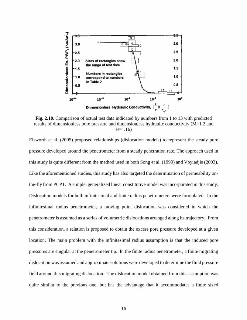
To validate the method proposed here, theoretically predicted results were compared with well-

documented field test data and experimental data from the calibration chamber system at Louisiana

State University. Ultimately, it was found that the test data agreed well with their theoretical

approach as shown in Fig. 2.10. The study also stressed that the method has a potential to

determine hydraulic conductivities from the continuous pore pressure measurements. It was

recommended by the authors to use the coupled theory of mixtures to predict the behavior of soils

within the range of 10-7 and 10-4 dimensionless hydraulic conductivity values, where the

dimensionless hydraulic conductivity is given by the expression �𝑘𝑘𝑣𝑣� � 𝑟𝑟

𝑟𝑟𝑟𝑟𝑟𝑟𝑟𝑟�. 𝑘𝑘 is the hydraulic

conductivity, 𝑣𝑣 is the penetration speed, 𝑟𝑟 is the radius of the penetrometer head and 𝑟𝑟𝑟𝑟𝑟𝑟𝑓𝑓 is the

radius of the reference penetrometer (1.784 cm)

. (a) (b)

Fig. 2.9. The effects of penetration speed (a) and confining stress (b) on excess pore

pressure response of PCPT

16

Fig. 2.10. Comparison of actual test data indicated by numbers from 1 to 13 with predicted results of dimensionless pore pressure and dimensionless hydraulic conductivity (M=1.2 and

H=1.16)

Elsworth et al. (2005) proposed relationships (dislocation models) to represent the steady pore

pressure developed around the penetrometer from a steady penetration rate. The approach used in

this study is quite different from the method used in both Song et al. (1999) and Voyiadjis (2003).

Like the aforementioned studies, this study has also targeted the determination of permeability on-

the-fly from PCPT. A simple, generalized linear constitutive model was incorporated in this study.

Dislocation models for both infinitesimal and finite radius penetrometers were formulated. In the

infinitesimal radius penetrometer, a moving point dislocation was considered in which the

penetrometer is assumed as a series of volumetric dislocations arranged along its trajectory. From

this consideration, a relation is proposed to obtain the excess pore pressure developed at a given

location. The main problem with the infinitesimal radius assumption is that the induced pore

pressures are singular at the penetrometer tip. In the finite radius penetrometer, a finite migrating

dislocation was assumed and approximate solutions were developed to determine the fluid pressure

field around this migrating dislocation. The dislocation model obtained from this assumption was

quite similar to the previous one, but has the advantage that it accommodates a finite sized

17

penetrometer. Further, the study incorporated piezocone indices (cone metrics) like 𝑄𝑄𝑡𝑡, 𝐹𝐹𝑟𝑟 and 𝐵𝐵𝑞𝑞

which stand for normalized tip resistance, sleeve friction ratio and pore pressure ratio respectively

into both the infinitesimal and finite radius dislocation models. Because the former suffered from

shortcomings, the finite radius penetrometer dislocation model was used for further interpretations.

Contour plots of permeability from each pair of indices Bq-Qt, Fr-Qt and Bq-Fr data are prepared

from the relationships indicated below, which are derived by combining both finite radius

penetrometer dislocation model and cone metrics.

tqD QB

K 1= (2.3)

−+

=

φtan11

1

r

tt

D FQ

QK (2.4)

+−= q

rqD BFBK 1

tanφ (2.5)

Where 𝐵𝐵𝑞𝑞 ,𝑄𝑄𝑡𝑡 and 𝐹𝐹𝑟𝑟 are cone metrics, 𝑡𝑡𝑡𝑡𝑡𝑡𝑡𝑡 is the coefficient of friction at the sleeve-soil

interface, 𝐾𝐾𝐷𝐷 is the dimensionless permeability given by (4𝑘𝑘𝜎𝜎′𝑣𝑣𝑜𝑜)/(𝑈𝑈𝑡𝑡𝛾𝛾𝑤𝑤), 𝑘𝑘 is permeability,

𝜎𝜎′𝑣𝑣𝑜𝑜 is the effective overburden pressure, U is the rate of penetration, a is the radius of the

penetrometer, and 𝛾𝛾𝑤𝑤 is the unit weight of water. Data computed from the above three equations

were correlated with known field data from two sites. It was concluded that the pair that contains

Bq performed well in estimating permeability, and particularly Bq-Qt yielded the closest result.

They also noticed that this method is applicable for a permeability range from 10-7 m/s to 10-4 m/s

and standard penetration rate of 2 cm/s. These ranges showed a shift to the right in the order of

magnitudes as compared to the ranges recommended in Song et al. (1999).

18

Lee at al. (2008) reported well-resolved measurements of hydraulic conductivity gathered from a

newly developed in-situ permeameter. By using this measurement, the study examined the effect

of tip-local disturbance and further examined the relative accuracy of hydraulic conductivity

determinations from soil classification correlations (Robertson, 1990, as cited in Lee, 2008) from

VisCPT measurements and from on-the-fly measurements of pore pressures using cone metrics

(Elsworth et al., 2005 as cited in Lee, 2008). This work was performed at the Geohydrologic

Experimental and Monitoring Site (GEMS) located in the floodplain of the Kansas River just north

of Lawrence, Kansas. For testing, the in-situ permeameter was fabricated with tips of variable

diameter (one with a sharp tip and the other with a large 4.5 cm length screen) to quantify the

effect of disturbance in the testing zone. To validate the hydraulic conductivities measured with

the in-situ penetrometers, calibration chamber tests were carried out with known hydraulic

conductivities. For both tip diameters, the in-situ permeameter results closely agreed with the

calibration chamber results, hence the in-situ permeameter results were used as a reference to

examine the relative accuracy of the other methods. Presumed hydraulic conductivities were

obtained from soil classification and grain size distribution (Robertson, 1990). VisCPT was used

to directly capture a continuous real-time image of the soil. The soil grain size (sand) is obtained

from image analysis of VisCPT and hydraulic conductivities are determined using Hazen formula.

On-the-fly determination of hydraulic conductivity was done based on an approximate solution

from the dislocation theory of finite radius penetrometer (Elsworth and Lee, 2005) without

performing dissipation test. Using Bq-Qt plot, the dimensionless hydraulic conductivity 𝐾𝐾𝐷𝐷 is used

to estimate the hydraulic conductivity, k. The following conclusions were made in this study:

19

a) The results from the in-situ permeameter suggested a minor influence of tip-local

disturbance. Thus, it indicated the feasibility of measuring hydraulic conductivity from

CPT tip configuration.

b) On-the-fly determination of hydraulic conductivity required the tip-local pore pressure

to be steady and partially drained.

c) If these conditions are satisfied, the on-the-fly PCPT sounding test has a practical

means of accurately determining hydraulic conductivity.

Song et al. (2010) carried out extensive numerical simulations based on finite element analysis and

proposed a more computationally and experimentally feasible method to determine hydraulic

conductivity from Piezocone penetration testing. The basis for this method was the coupled

relation of stress, deformation, pore water pressure and hydraulic conductivity. For this purpose,

a coupled equation of mixtures derived by Abu-Farsakh (1998), as cited by Song et al. (2010), was

used and modified cam-clay constitutive modeling is adopted to mimic the stress-strain behavior

of the soil. Furthermore, it was shown that the response of soils during PCPT is a coupled response

of M, λ, κ, pore pressure and hydraulic conductivity, where M is the slope of the critical state line,

𝜆𝜆 is the slope of the critical state line in 𝜈𝜈 − 𝑙𝑙𝑡𝑡𝑙𝑙′ axis, and 𝜅𝜅 is the slope of the recompression line

in 𝜈𝜈 − 𝑙𝑙𝑡𝑡𝑙𝑙′ axis. The first two parameters indicate the stress-deformation characteristics. The

effect of λ on the both pore water pressure and hydraulic conductivity of soils was considered to

be negligible and thus it was discarded from further consideration. For this, it was reasoned that

the constrained modulus corresponding to λ is much lower than that to κ, and thus a relatively

smaller stress change is required for a given strain level in strain-controlled tests like PCPT. For

such small induced stresses, the induced pore water pressure will be small and hence have

negligible use in estimating hydraulic conductivity of the soil. A unique technique from the

20

previous works (Song et al., 1999; Voyiadjis et al., 2003) called variable separation was used in

order to uncouple each variable and write one in terms of the other. Using this technique, explicit

equations for pore water pressure in terms of κ, k and M were derived. From these equations and

from mathematical manipulations, a logic that can estimate the hydraulic conductivity of soils as

a function of u, κ and M is expressed as shown in [Eq. (2.6)].

+−−

+−−−

=

0.1κlog160)0.1(3507.893,1

0.1κlog160)0.1(350002436.01

Mu

Muk (2.6)

where:

k is the hydraulic conductivity in m/sec,

u is the excess pore pressure in kPa,

κ is the recompression slope of void ratio vs. natural log pressure curve (dimensionless),

M is the slope of the critical state line (dimensionless).

The authors have indicated the following limitations of this equation:

a) Not applicable to sensitive clays

b) Applicable to λ/κ ratio from 0.1-0.2

c) Applicable for hydraulic conductivity range from 5x10-9 to 5x10-5 cm/s

d) Soils are assumed in a normally consolidated state

e) Assumed isotropic hydraulic conductivity

2.4 Conclusion

Estimation of hydraulic conductivity from PCPT can be done either by theoretically interpreting a

dissipation curve or on-the-fly from the pore pressure response recorded during piezocone testing.

The theoretical interpretation of dissipation curves is based on the prediction of the relationship

21

between the time factor and the excess pore pressure as penetration of the cone is halted. The key

findings from the reviewed literatures are summarized as follows:

a) Dissipation is controlled mostly by the horizontal coefficient of consolidation

b) The prediction of the initial excess pore pressure is very important

c) The rigidity index is also important in theoretical modeling of dissipation curves

d) Most of the theories assume undrained condition

Analytical methods to interpret piezocone penetration data in order to determine hydraulic

conductivity on-the-fly are also available. These methods rely on the assumption of a partial

drainage condition in which excess pore pressure generation and dissipation occur at the same time

(Song et al. 1999, Voyiadjis and Song 2003, Elsworth and Lee 2005). These methods use

sophisticated numerical techniques and the associated costs are quite high. However, the semi-

empirical equation proposed by Song and Pulijala (2010) is simple to use and provides an efficient

way of determining hydraulic conductivity.

22

3 PRELIMINARY EVALUATION OF HYDRAULIC CONDUCTIVITY BASED ON LABORATORY TEST AND PCPT

3.1 Background

In this chapter, preliminary evaluation of hydraulic conductivity of soils using laboratory data and

piezocone penetration test data is presented. Relevant data for all analyses carried out in this

research were obtained from the Nebraska Department of Transportation (NDOT). Prior to the

investigation of hydraulic conductivity, data collected from NDOT were organized so that data

analysis could be executed quite easily.

The equation proposed by Song and Pulijala (2010) with some modifications and form changes,

has been used to analyze the hydraulic conductivity based on PCPT data. In addition to this,

hydraulic conductivity was also analyzed based on laboratory test data. From the collected PCPT

and laboratory data, it has been determined that a majority of soil in Nebraska is overconsolidated

soil as depicted by the OCR values of the soils and the negative or small magnitude of pore pressure

measured from PCPT. However, it can be recalled from the previous literature discussion above,

the equation proposed by Song and Pulijala (2010) is intended to be used for normally consolidated

soils. To apply this preexisting equation to the specific soil examined in this project, measured

excess pore pressure from PCPT should be adjusted for the overconsolidated soil condition before

it is introduced into the equation. The details of the activities done in this research report are

presented and discussed herein after.

23

3.2 Data Collection and Organization

Piezocone penetration test results of several projects along with their borehole log data were

acquired from NDOT. The piezocone penetration data consisted of the cone resistance, the sleeve

friction resistance and the pore pressure measured at u2 position. The data collected from NDOT

also consisted of laboratory test data of soil samples recovered from PCPT test holes. The primary

target parameters from laboratory tests were the consolidation test results, which include the

coefficient of consolidation, compression and recompression indices (Cv, Cc and Cr respectively).

Data collected from a total number of 28 projects were reviewed. Of the data obtained from the 28

projects, only 15 projects were utilized due to laboratory data or borehole log data that didn’t

contain the primary target parameters needed. The comparison of laboratory determined hydraulic

conductivity and PCPT based hydraulic conductivity was done at discrete depths or points. This is

because the laboratory tests are based on soil samples that are collected at discrete depths. Hence,

the data available for comparison was dependent on the number of laboratory tests carried out for

a given borehole. The depth of the groundwater table for each project was also collected and

organized either directly from the borehole log or indirectly from the pore pressure distribution

measured during PCPT. The summary of the data used is shown in Appendix A.

3.3 Estimation of Hydraulic Conductivity from Laboratory Test Results

Before the estimation of the adjustment factors that should be applied to the measured excess pore

pressure from PCPT, hydraulic conductivity estimation based on laboratory results was performed.

In this regard, consolidation test results were used to determine the hydraulic conductivity of the

soil samples collected at different specific depths in each borehole. The hydraulic conductivity of

a soil can be determined from a consolidation test using [Eq. (3.1)] as shown below.

24

wvvmck γ= (3.1)

where k is hydraulic conductivity (L/T), mv is coefficient of volume compressibility (1/F) and γw

is unit weight of water (F/L3). The coefficient of volume compressibility is given by:

)'()1( σ∆∂+∂−

=o

v eem (3.2)

where e and eo are void ratio and initial void ratio respectively, and σ’ is the effective vertical

stress. The change in void ratio (Δe) for normally consolidated soil can be computed using [Eq.

(3.3)].

∆+=∆

o

ocCe

σσσ ''

log (3.3)

where Cc is compression index. The final void ratio after an application of Δσ’ vertical stress is

given by eee o ∆−= .

Coefficient of consolidation, compression index and initial void ratio were calculated directly from

the given consolidation test data from NDOT. But, the value of volumetric modulus of

compressibility (mv) was computed indirectly using [Eq. (3.2) & (3.3)]. Rearranging [Eq. (3.2)].

as shown in [Eq. (3.4)] and plotting void ratio (e) with change in effective stress (Δσ’), values of

mv were calculated for a level of stress equivalent to the cone resistance (qt). A sample plot

prepared for project 2-6(119) RO-1 and a computation of mv at a depth of 7.43 m (24.76 ft) below

the ground surface are discussed below.

Table 3.1 Computation of mv from the given consolidation test results

σo' Δσ’ (σo'+Δσ')/σo' log((σo'+Δσ')/σo') Cclog((σo'+Δσ')/σo') e e/(1+eo) 134.88 0 1.00 0.000 0.000 0.45 0.310 134.88 600 5.45 0.736 0.081 0.369 0.254 134.88 1200 9.90 0.995 0.110 0.340 0.234 134.88 1800 14.35 1.157 0.127 0.323 0.222 134.88 2400 18.79 1.274 0.140 0.310 0.213

25

134.88 3000 23.24 1.366 0.150 0.300 0.206 134.88 3600 27.69 1.442 0.159 0.291 0.200 134.88 4200 32.14 1.507 0.166 0.284 0.196 134.88 4800 36.59 1.563 0.172 0.278 0.191

N.B. stresses are in kPa

)'(1σ∆∂

+∂−= o

v

ee

m (3.4)

Fig. 3.1. Stain versus change in effective stress

From Fig. 3.1, the instantaneous slope (which in our case is the same as mv) can be found by taking

the first order derivative of void ratio with change in effective stress as indicated in [Eq. (3.4)].

Thus, ( ) ( )'0311.0'

0311.0σσ ∆=∆

−−=vm . Once we know the cone tip resistance, the value of mv

is obtained by substituting the cone tip resistance in Δσ’. For instance, at a depth of 7.43 m (24.76

ft), the cone tip resistance was found to be 2496 kPa. Then, mv is calculated as

( ) 510246.1kPa 24960311.0 −== xmv 1/kPa ( 51059.8 −x 1/psi). The coefficient of consolidation for

the soil sample at this depth was found to be 61025.7 −x m2/s (6.74 ft2/d). The hydraulic

conductivity of the soil can be then computed by using [Eq. (2.1)] as:

ft/d 1051.2m/s 1086.8)81.9)(10246.1)(1025.7( 41056 −−−− ==== xxxxmck wvv γ

e/(1+eo)= -0.031ln(Δσ') + 0.4517R² = 0.9994

0.15

0.17

0.19

0.21

0.23

0.25

0.27

0.29

0.310 1000 2000 3000 4000 5000 6000 7000

e/(1

+eo)

Δσ', kPa

26

In a similar fashion, the hydraulic conductivity at different depths where complete laboratory

results exist was calculated. A table showing hydraulic conductivity computed from laboratory

results is provided in Appendix B of this report. As a sample, Table 3.2 shows the hydraulic

conductivity estimated from laboratory test results for project 2-6(119) RO-1.

Table 3.2. Hydraulic conductivity based on laboratory test results for project 2-6(119) RO-1

Depth Cv eo Cc Cr σo σp qt mv k k m m2/s kPa kPa kPa 1/kPa m/s ft/d

2.34 7.08E-06 0.85 0.35 0.03 47.14 428.54 2161 3.52E-05 2.44E-09 6.92E-04 3.84 1.20E-05 0.76 0.38 0.04 68.26 449.28 1871 4.65E-05 5.49E-09 1.56E-03 5.96 7.61E-06 0.74 0.27 0.03 108.34 428.54 1631 3.86E-05 2.88E-09 8.18E-04 7.43 7.25E-06 0.45 0.11 0.02 134.88 331.68 2496 1.25E-05 8.86E-10 2.51E-04

3.4 Estimation of Hydraulic Conductivity Based on PCPT

As it has been discussed in chapter one, one of the applications of the cone penetration test is for

the determination of hydraulic conductivity. Although hydraulic conductivity can be estimated

based on the traditional dissipation test or on the fly, the on the fly techniques are more

advantageous in providing a quick and continuous profile of hydraulic conductivity with depth.

Song and Pulijala (2010) came up with a simple semi-analytical approach to determine hydraulic

conductivity on the fly as a function of excess pore pressure at the u2 position. The critical state

line slope (M) and slope of elastic swelling line (κ) are also the variables in this equation. A slightly

modified form of the equation proposed by Song and Pulijala (2010) was used for the estimation

of hydraulic conductivity based on PCPT and is shown in [Eq. (3.5)].

0564.1

22.095,282

1)M,(

−= u

f

k

κ

(3.5)

where,

27

k is hydraulic conductivity in m/s

u is the excess pore pressure measured at u2 position

( ) ( )( )11.0/log32.0 32.62M25.345 )M,( +−+= κκf

M is the slope of the critical state line in p’-q axis

κ is the slope of elastic swelling line 'ln pv − in axis

Fig. 3.2 Excess pore pressure Vs hydraulic conductivity for different values of M and 01.0=κ based on Song and Pulijala (2010)

It should be noted however, [Eq. (3.5)] is only valid for hydraulic conductivity ranging from 4105 −x

m/s to 9105 −x m/s. When the ratio of uf )/M,( κ is less than unity, hydraulic conductivity of a given

soil is less than 9105 −x m/s.

For the sake of providing a continuous hydraulic conductivity profile, whenever [Eq. (3.5)] gave

an undefined hydraulic conductivity, the upper bound hydraulic conductivity (i.e. 9105 −x m/s) was

assumed. Fig. 3.2 shows the relationship between hydraulic conductivity and excess pore pressure

using [Eq. (2.5)]. 3.3 shows a sample calculation of hydraulic conductivity based on PCPT data

for project 2-6(119) RO-1. A similar procedure is followed for the rest of the projects.

28

Table 3.3. Hydraulic conductivity based on PCPT for project 2-6(119) RO-1

3.4.1 Strength and Compressibility Parameters (M and κ)

The slope of the critical state line is dependent on the angle of friction of a given soil. To get the

proper value of the critical state line slope profile with depth, it is necessary to know the variation

of the angle of friction of the soil with depth. There are several ways by which the value of angle

of internal friction of a given soil can be identified. These methods mainly rely on laboratory tests

or correlations from field tests.

Assessment of the laboratory results for the different projects indicated that the soils tested in

almost all projects are mainly fine grained soils. The best means of finding the angle of friction of

fine grained soils is to perform a triaxial test using high quality undisturbed soil samples

(Robertson and Cabal 2010). Available correlations based on field tests mainly focus on sands and

normally consolidated fine grained soils. In the absence of a reliable value, Robertson and Cabal

(2010) recommended to assume a value of 28o for clays and 32o for silts. Based on the SBTn

(normalized soil behavior type) chart provided by Robertson (1990, 2010), most of the soils were

categorized in zone 3, 4, 5 and 9. Zones 3, 4, 5 and 9 stand for clay, clay-silt mixture, sand-silt

mixture and very stiff fine grained soil respectively. As most of the soil fell in either the clay or

silt category, an average angle of internal friction of 30o was assumed. The critical state line slope

GWT= 2.00 m

Depth Pwp, u2

Static Pwp

Ex Pwp Φ’ M Cr κ k k

m kPa kPa kPa m/s ft/d 2.34 40.20 3.34 36.86 30 1.20 0.03 0.014 3.15E-05 8.93 3.84 103.50 18.05 85.45 30 1.20 0.04 0.018 1.14E-05 3.23 5.96 206.70 38.80 167.90 30 1.20 0.03 0.012 4.96E-06 1.40 7.43 68.10 53.22 14.88 30 1.20 0.02 0.010 8.94E-05 25.34

29

(M) was computed using [Eq. (3.6)]. For an angle of internal friction (ϕ’) = 30o, the critical state

line slope (M) will be 1.20.

'sin3'sin6φφ

−=M (3.6)

The slope of the elastic swelling line (κ) was calculated from the recompression index (Cr), which

was obtained from a consolidation test as shown in [Eq. (3.7)].

303.2

rC=κ (3.7)

3.4.2 Adjustment Factors to Compensate for Overconsolidation Effect

The equation proposed by Song and Pulijala (2010) is applicable to normally consolidated soils.

Overconsolidated clays and very dense fine or silty sands give very low or even negative pore

pressure readings at the pore pressure sensor behind the cone or at the u2 position (Lunne et al.

1997). Therefore, if one uses the equation of Song and Pulijala without using proper adjustment

factors for the pore pressure measured for soils stipulated above, then the hydraulic conductivity

estimation will result in higher values. As evidence, comparison of the hydraulic conductivity

estimated based on laboratory test results (Table 3.2) and based on PCPT (Table 3.3) clearly shows

that the estimated hydraulic conductivity values by the equation are larger than those estimated

based on laboratory results. To close the gap between the two estimations, there was a need to

apply adjustment factors to compensate for the overconsolidation effect. To find out the proper

adjustment factors, the following methodology was adopted:

1. Back analysis of the excess pore pressure that should be used in [Eq. (3.5)] was done by

equating the hydraulic conductivity based on laboratory test results with the Song and

Pulijala’s equation.

30

2. Then, the adjustment factors were computed by dividing the excess pore pressure

obtained in step (1) by the measured excess pore pressure based on PCPT.

3. A correlation was determined between the adjustment factors obtained in step (2) and

SBTn chart parameters Qt, Fr and Bq (Robertson 2010). These parameters are chosen

because they reflect the type of soil penetrated during PCPT. From this correlation, a

unique adjustment function was proposed which mainly relies on the type of the soil.

(3.8)

where, Qt is normalized cone resistance, Fr is normalized friction ratio, and Bq is pore pressure

ratio. qt is corrected cone resistance, fs is sleeve friction and u2 is pore pressure measured behind

the cone. Table. 3.4 shows how the adjustment factors are computed on the basis of equating

laboratory test result based hydraulic conductivity with [Eq. (3.5)].

Table 3.4. Computation of adjustment factors and SBTn parameters

Depth Pwp, u2

Hydro static Pwp

Ex Pwp

Adj. Factor

(C)

Adj. Ex

Pwp k (PCPT) k (Lab) Qt Fr Bq SBTn

Zone

m kPa kPa kPa kPa m/s m/s % 2.34 40.20 3.34 36.86 16.44 606.18 2.43E-09 2.44E-09 51.40 5.89 0.02 4 3.84 103.50 18.05 85.45 6.89 588.59 5.48E-09 5.49E-09 32.95 3.61 0.05 4 5.96 206.70 38.80 167.90 3.68 617.35 2.88E-09 2.88E-09 20.76 4.76 0.11 4 7.43 68.10 53.22 14.88 42.45 631.76 8.83E-10 8.86E-10 28.16 5.14 0.01 4

The adjustment factors (designated as C) were computed in the same fashion for the remaining 14

projects. After compiling the adjustment factors and the SBTn parameters at each depth for the 15

projects, a satisfactory correlation was obtained between the two. A single non-dimensional factor

(designated as N) which was a function of Qt, Fr and Bq was found to have the best correlation

with the adjustment factors among any combinations of Qt, Fr and Bq. The expression for N is

given below in [Eq. (3.9)].

vo

vott

qQ'σσ−

= %100xq

fFvot

sr σ−=

vot

oq q

uuBσ−−

= 2

31

r

qt

FBQ

N = (3.9)

In [Eq. (3.9)], one should note that the absolute value of N should be taken while evaluating the

Fig. 3.3. Correlation between adjustment factors and non-dimensional factor N

adjustment factors, because in some instances (e.g. very stiff soil strata) the value Bq will be

negative. The proposed correlation between N and C is shown in Fig. 3.3 and the complete data

used for this analysis is shown in Appendix C.

From the correlation, the adjustment factors can be estimated using the relationship shown in [Eq.

(2.10)]. Then, hydraulic conductivity can be estimated from [Eq. (3.5)] by multiplying the

measured pore pressure (u) with the adjustment factors estimated from [Eq. (3.9)].

65.0025.4 −±= NC (3.10)

When the measured excess pore pressure is negative, the negative of the adjustment factor

computed from [Eq. (3.9)] should be used and vice versa. The adjustment factors can be estimated

on the fly once the level of the ground water table is fixed. Another advantage of [Eq. (2.10)] is

that adjustment factors can be estimated in a continuous profile as far as the non-dimensional

32

normalized SBTn parameters are computed. Appendix D shows the estimation of hydraulic

conductivity from PCPT after applying adjustment factors.

3.5 Sample Hydraulic Conductivity Profiles with Depth

In this section, sample hydraulic conductivity profiles plots are shown. These plots include the

variation of hydraulic conductivity with depth estimated by PCPT before adjustments and after

adjustment. In Fig. 3.4 the dotted rectangular shape indicates the hydraulic conductivity ranges

estimated from consolidation test results. There is a significant deviation between the unadjusted

hydraulic conductivity and laboratory test result. However, after applying the adjustment factors,

the hydraulic conductivity deviates by an order of 1~2 from the measured hydraulic conductivity

obtained from laboratory test.

Project 2-6(119) RO-1 Project 2-6(119) RO-3

33

Fig. 3.4. Predicted hydraulic conductivity profiles with depth based on PCPT

Project 2-6(1027) Project 80-9(862)

Project 75-2(165) W Project 80-9(839) 148-1

34

4 ADDITIONAL EVALUATIONS ON THE CORRELATION AND CASE STUDIES

4.1 Introduction

Further evaluation and modification was done on the correlation obtained from the previous

assessment in chapter 3. The evaluation has been done regarding the difference between positive

and negative measured pore pressure on the hydraulic property of Nebraska soil. Moreover, the

evaluation process included the investigation of the data points that are used for the estimation of

the correlation between the non-dimensional factor N and adjustment factor C by plotting those

data points on the SBTn (normalized soil behavior type) chart proposed by Robertson (2010).

Based on this evaluation, a slight modification was made on the previously established relation

between N and SBTn parameters (Qt, Fr and Bq).

Case studies from well documented sites from the USA, Canada and South Korea are also included

in this report. From these studies, quite satisfactory results are obtained for the estimation of

hydraulic conductivity on the fly modified Song and Pulijala (2010). Hydraulic conductivity

estimated based on the SBTn chart is compared with the results obtained from the proposed

correlation.

Finally, an attempt was made to produce software to assist in the determination of hydraulic

conductivity on the fly using visual basic for applications (VBA). Though the program has not

progressed to completion, the foundational work completed so far regarding the VBA-based

program is presented at the end of this report.

35

4.2 Evaluation of Data Points with negative and Positive Pore Pressure Ratio (Bq)

4.2.1 Qualitative Evaluation In the previous evaluation, an absolute value of the non-dimensional parameter N was taken

without proper justification. The previously proposed N and its correlation with C was taken as:

r

qt

FBQ

N = (4.1)

65.0025.4 −±= NC (4.2)

where Qt, Bq and Fr are normalized cone resistance, pore pressure ratio, and friction ratio

respectively. It was assumed that if the measured excess pore pressure assumes a negative sign

then the negative of the computed adjustment factor from [Eq. (4.2)] should be considered.

Moreover, through this correlation, it was explicitly shown that the sign of Bq is minimally

important for the prediction of adjustment factors. Qualitatively, the effect of the sign of Bq on

hydraulic properties can be discussed with the help of the SBTn chart proposed by Robertson

(2010), as shown in Fig. 4.1.

Fig. 4.1. Normalized soil behavior type (SBTn) chart (after Robertson 2010)

Zone 9 Zone 3 (OC side)

36

From Fig. 4.1, which shows two regions in the SBTn chart where one is zone 3 (overconsolidated

side) and the other is zone 9 (very stiff fine grained soil region). Obviously, a large negative Bq is

expected in zone 9 due to soils in this zone showing significant dilative characteristics. Whereas

for zone 3, a small negative or small positive Bq is expected in the overconsolidated side. If one

compares the upper and lower bound hydraulic conductivity of these two regions, zone 3 will have

a value of 10 x 10-10 m/s to 10 x 10-9 m/s while zone 9 has a value of 1 x 10-9 to 1 x 10-7 m/s. From

this, it is implied that though the sign of their Bq values can be substantially different, the hydraulic

characteristics are still comparable.

Based on the above explanation, further evaluation can be made using the typical trends of excess

pore pressure dissipation discussed in Burns and Mayne (1998). Now, consider Fig. 4.2 which

shows the trends of dissipation of excess pore pressure measured at the u2 filter location for

normally and overconsolidated soils. Normally and lightly overconsolidated soils (contractive

soils) show monotonic dissipation with time. On the other hand, moderately and heavily

overconsolidated soils (dilative soils) display lower value of pore pressure before reaching a peak

pore pressure and dissipate monotonically as witnessed in normally or lightly overconsolidated

soils as shown in Fig. 4.2.

Fig. 4.2. Dissipation of pore pressure for contractive and dilative soils (adapted from Burns and Mayne 1998)

adjustedu

measuredu

t

2uMonotonic pore pressure dissipation in normally consolidated soils (contractive)

Pore pressure dissipation in heavily overconsolidated soils (dilative)

37

From Fig. 4.2, one can see that the hydraulic property of the two soils is similar, since the

monotonic dissipation curves are parallel (dissipation after peak value for the OC soil). However,

the initial pore pressure measured in the dilative soil is lower than the one measured in contractive

soil due to their inherent characteristics. When adjustment factors are applied to the measured pore

pressure (umeasured in Fig. 4.2) of the dilative soil, it will be transformed to an initial pore pressure

that would have been measured from an “equivalent” normally consolidated soil having an initial

pore pressure designated as uadjusted in Fig. 4.2.

Going further, now consider a hypothetical initial small and large negative pore pressure measured

from heavily overconsolidated soils with same hydraulic properties as shown in Fig. 4.3 though

such dissipation trend has not been particularly noticed from literatures.

Fig. 4.3. Hypothetical dissipation of pore pressure in heavily overconsolidated soils

From Fig. 4.3, the adjustment factor required to transform a heavily overconsolidated soil with

small negative excess pore pressure (umeasured (A)) will be larger than the adjustment factor required

to change the one with large negative value (umeasured (B)). This is because the small negative pore

pressure has lower magnitude compared to the larger negative pore pressure, so it requires a higher

adjustment factor. From this, it can be claimed that for smaller positive and negative pore

)(Bmeasuredu

)( Ameasuredu

adjustedu

t

2u

38

pressures, the larger the adjustment factors expected and the larger the positive and negative pore

pressures are, the smaller the adjustment factor needs to be. Therefore, if this explanation holds

true, then the sign of Bq has less importance, and considering absolute value N, which is a function

of Bq, is logical.

4.2.2 Quantitative Evaluation

The data set used for the derivation of the correlation between C and N is employed to verify the

qualitative explanation given in 4.2.1 of this report. A total of 72 data points have been used to

define the correlation in the previous evaluation in chapter 3. Among these 72 data points, 16 data

points consisted of negative Bq, while the rest consisted of positive Bq. Each data set (one with

positive Bq and the other with negative Bq) was organized independently along with their respective

adjustment factors. Then, N is computed for each data set. For the negative Bq category, both

computed N and C assumed negative values whereas the positive Bq category assumed positive N

and C. Based on the discussion in the previous section, rather than taking the absolute value of Bq,

this report intends to take the square of Bq. However, this consideration will be analyzed

subsequently. N is modified to N* as:

2* qr

t BFQ

N = (4.3)

Before data analysis is carried out, all 72 data points with Qt and Fr values are plotted on the SBTn

chart as shown in Fig. 4.4. The plot shows that all data points used in the correlation are relevant,

since most of the points lie in the overconsolidated soils region. This may be desirable, as the

correlation seeks to find an adjustment factor to the pore pressure measured for overconsolidated

soils. Fig. 4.5(a) shows N* versus C for the two data sets (i.e. one with positive Bq and the other

with negative Bq). To check the validity of the assumption made in the qualitative evaluation, the

39

mirror image of the data sets for negative Bq is taken to the positive side as shown in Fig. 4.5(b),

and a trend line is obtained for each case.

Fig. 4.4. Classification of soils in Nebraska using SBTn chart

(a) (b)

Fig. 4.5. C vs modified N for negative and positive Bq data points (a) without reflection (semi log scale) (b) by reflection about N* axis (full log scale)

40

Referring Fig. 4.5(b), best fit power functions for positive and negative Bq are almost parallel.

Moreover, the ratio of the estimated adjustment factors from the two functions is obtained to be

approximately 1.50 and hence, it can be said that the deviation in the adjustment factors is not

significantly large. More importantly, through the quantitative evaluation, it is shown that the sign

of Bq has almost no effect on the prediction of adjustment factors. Considering this, a single

modified trendline that encompass both data sets is proposed in Fig. 4.6.

Fig. 4.6. C vs N* incorporating both negative and positive Bq

The modified correction equation with a coefficient of determination (R2 = 0.8416) is given by:

( ) 38.0*80.1−

= NC (4.4)

where C and N* are adjustment factor and modified factor N, respectively.

41

4.3 Evaluation of the Correlation for other Sites

4.3.1 Yangsan Mulgeum, Korea (Dong A Geology 1997)

This site is the old delta area of the Nakdong River. The soils are primarily young alluvial deposits.

(a) (b)

Fig. 4.7. (a) SBTn classification and range of hydraulic conductivity (b) Estimated hydraulic property profile with depth for Yangsan, Korea (data obtained from Dong A. Geology 1997)

According to Kim (2005), the area has approximately 10,000 years of sedimentary history, and the

self-weight consolidation is still under progress. This area consists of clayey and silty fill materials,

sedimentary layers consisting of clay, silty sand, silty clay, silt, sand, and gravel from the top. Pore

pressure dissipation test using PCPT shows the coefficient of consolidation is (2-6) ×10-7 m2/sec,

and no other consolidation properties were provided.

42

Based on Robertson (2010), the soil is classified as silty clay to sandy silt with a hydraulic

conductivity range from 3 x 10-9 m/s to 1 x 10-5 m/s as shown in Fig. 4.7(a). The ground water

table is reported to be at a depth of 1 m.

From Fig. 4.7(a), the data points lean to the sensitive fine grained soils side. Some data points are

also inside the normally consolidated soils zone. In Fig. 4.7(b), the estimated hydraulic

conductivity shows good agreement with the laboratory measured hydraulic conductivity

(indicated by the rectangular dotted plot), particularly towards deeper depths. Additionally, the

estimated hydraulic conductivity is to the right of the measured hydraulic conductivity. This can

be considered reliable, because it is common to have substantial deviation in laboratory and field

hydraulic conductivity. Moreover, the unadjusted and adjusted hydraulic conductivity profiles are

very close to each other. This may be because the soil is normally consolidated.

4.3.2 Frazer River, Canada (Crawford and Campanella 1991)

The area is located about 25 km South East from Vancouver on highway 99. The surface of this

area is mostly floodplain, and the stratigraphy of the ground shows inter-bedded sand seams or

peat layers. The subsurface soils are relatively uniform with a natural water content of about 45%

and the liquid limit around 36%. According to consolidation test results, coefficients of

compressibility, initial void ratios, vertical coefficients of consolidation, horizontal coefficients of

consolidation, constrained modulus, and permeability are 0.3-0.5, 1.1-1.8, (0.6-2.8) × 10-7 m2/s,

(0.7-7) × 10-7 m2/s, 1800-4 000 kPa, and (0.8-1.2) × 10-9 m/s respectively. The soil in the site is

reported to be slightly overconsolidated to normally consolidated. In addition, from vane shear test

results, it is reported that the soil shows high sensitivity in deeper depths. The ground water table

is reported to be close to the ground surface. Based on Robertson (2010), the soil is classified as

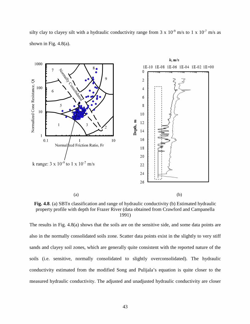
43

silty clay to clayey silt with a hydraulic conductivity range from 3 x 10-9 m/s to 1 x 10-7 m/s as

shown in Fig. 4.8(a).

(a) (b)

Fig. 4.8. (a) SBTn classification and range of hydraulic conductivity (b) Estimated hydraulic property profile with depth for Frazer River (data obtained from Crawford and Campanella

1991)

The results in Fig. 4.8(a) shows that the soils are on the sensitive side, and some data points are

also in the normally consolidated soils zone. Scatter data points exist in the slightly to very stiff

sands and clayey soil zones, which are generally quite consistent with the reported nature of the

soils (i.e. sensitive, normally consolidated to slightly overconsolidated). The hydraulic

conductivity estimated from the modified Song and Pulijala’s equation is quite closer to the

measured hydraulic conductivity. The adjusted and unadjusted hydraulic conductivity are closer

44

in the shallower depths, which might imply the existence of normally consolidated soils, though

there is significant deviation at deeper depths. This may be due to the increased sensitivity and

effect of confining pressure in deeper depths. Moreover, the adjusted hydraulic conductivity ranges

match those proposed by Robertson (2010) for zone 4 soils.

4.3.3 Cheongna (Section 1), Incheon, Korea (Kaya Engineering Co. 2007)

This area consists of overconsolidated soil in the upper layer and normally consolidated soil in the

lower layer. Typical geotechnical properties show that the total unit weight is 1.57-1.95 t/m3, liquid

limit is 30-50%, natural water content is 20-40%, classification is CL, vertical coefficient of

consolidation is (1-10) × 10-7 m2/sec, horizontal coefficient of consolidation is (3-50) × 10-7 m2/sec,

coefficient of compressibility is 0.2-0.4, the depth of the soft layer is about 10 m, hydraulic

conductivity is 4.82 x 10-8 m/s - 8.96 x 10-7 m/s, and OCR is 0.62~5.50. The soil in this area

primarily falls under 3, 4 and 5. Most the data points are within the boundary between zones 3 and

4 which designates clay to silty clay soils. The hydraulic conductivity for these zones based on the

SBTn chart ranges from 10-10 m/s to 10-7 m/s. Referring to Fig. 4.9(a), most the data points are in

the overconsolidated soil zones. Some scattered data points show the soils are normally

consolidated and somewhat sensitive. With the proper adjustment supplied to the unmodified Song

and Pulijala (2010) equation based on the SBTn parameters, the estimated hydraulic conducted

shows good agreement with the reported hydraulic conductivity of this area.

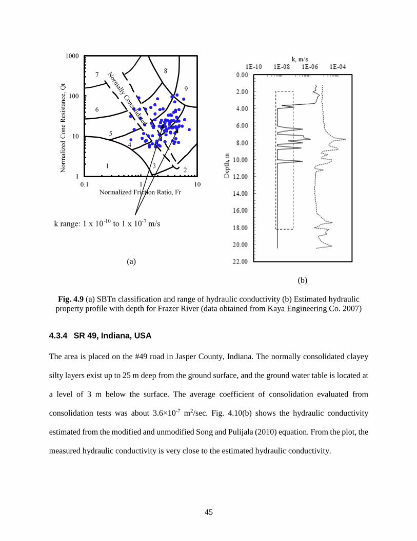
45

(a)

(b)

Fig. 4.9 (a) SBTn classification and range of hydraulic conductivity (b) Estimated hydraulic property profile with depth for Frazer River (data obtained from Kaya Engineering Co. 2007)

4.3.4 SR 49, Indiana, USA The area is placed on the #49 road in Jasper County, Indiana. The normally consolidated clayey

silty layers exist up to 25 m deep from the ground surface, and the ground water table is located at

a level of 3 m below the surface. The average coefficient of consolidation evaluated from

consolidation tests was about 3.6×10-7 m2/sec. Fig. 4.10(b) shows the hydraulic conductivity

estimated from the modified and unmodified Song and Pulijala (2010) equation. From the plot, the

measured hydraulic conductivity is very close to the estimated hydraulic conductivity.

46

(a) (b)

Fig. 4.10 (a) SBTn classification and range of hydraulic conductivity (b) Estimated hydraulic property profile with depth for Frazer River (data obtained from Kaya Engineering Co. 2007)

4.4 Hydraulic Conductivity Determination Program A goal in this project for the implementation of the correction factors is to code a spread sheet that

allows NDOT engineers and field employees to easily apply the correction factors to the PCPT

output to obtain a continuous hydraulic conductivity profile. This program should be simple to use

for anybody with access to the PCPT output and the values for a few assumed parameters. This

section details the progress made in “version 1” of the program, which will serve as a foundation

for smoother and more capable future versions.

47

4.4.1 Program Development (Version 1)

This program was developed using Excel’s built in language, Visual Basic for Applications

(VBA). This is a language developed by Microsoft to interface well with Excel. This language

enables a spreadsheet to be coded with a more powerful version of the macros that are commonly

found within a cell. For example, the spreadsheet can be designed to automatically perform a series

of tasks or display a user form that provides a graphic user interface that is easier to operate than

directly interacting with an Excel datasheet.

VBA works in conjunction with a standard Excel spreadsheet, which serves as the backbone of the

program. Traditional macros are still used on the spreadsheet for the intermediate calculations

required to obtain the correction factors. For the initial input, the user selects the data file from the

PCPT instrument output using the user form and inputs a few assumed parameters. This Visual

Basic component of the Excel document then uses this information to provide a starting point for

the standard Excel sheet containing macros. That sheet then runs the calculations to determine

adjustment factors and determine a final hydraulic conductivity value. This can then be graphed

and displayed on the user form. This functionality will be explained in more detail in the

subsequent sections.

4.4.2 User Form

Visual Basic for Excel was used to allow for the input and interpretation of data obtained from

PCPT testing. Because the method relies on a few assumed variables, the program’s user form has

text boxes to input the depth of the groundwater table, internal friction angle phi, and

recompression index Cr. The goal of this program is to accept input of the output from the PCPT

device, which will be in the format of an excel file—specifically .CSV. Additionally, it will accept

48

the user’s input of our method’s assumed parameters: Ground water table depth, ϕ, and Cr. These

inputs will take place on the program’s user form, which is shown in Fig. 4.11.

. Fig. 4.11. VBA user form

When the “Select Data File” button is selected, a window pops up that allows the user to select the

.CSV (or other Excel file type) from their computer that contains the PCPT output. This window

should look familiar, and is shown in Fig. 4.12. Currently, the order of the columns in the source

must be in the standard H, qc, fs, and u2 order from left to right. These columns are copied from

the source and pasted into the program’s worksheet. When copying the data, the program moves

downward along these first four columns until it finds an empty row. This allows the program to

be used for any depth. These first four columns copied from the source are shown to the left of the

49

red line on Fig. 4.13, and the intermediate calculations are performed to the right of the red line

using macros embedded in the cells.

Fig. 4.12. User selection of PCPT

Referring again to Error! Reference source not found. 4.14, the GWT depth, 'φ , and Cr are

typed into textboxes in the user interface. While the correction factors developed in this research

use GWT depth in meters, M instead of 'φ , and κ instead of Cr, the input units on the user form

were chosen because they are more commonly used in industry practice. The user’s inputs are

immediately converted to GWT depth in meters, M, and κ so that the equations developed in this

research can be directly used. Once these inputs are included in the intermediate calculations, the

final adjusted hydraulic conductivity profile has been determined. This profile is subsequently

plotted for the user when they select the “Plot” button on the user form. Currently there are bugs

50

in the functionality of this element, but an edited image of the plotted output that will be available

in version 2 of the program is depicted in Fig. 4.14.

Fig. 4.13. Background

The reset button on the user form deletes the GWT, phi, and Cr values from the spreadsheet, along

with the four columns imported from the PCPT readings.

4.4.3 Future Capabilities

Ideally, the code will become more generalized. As mentioned order, the columns from the PCPT

source data must be in the order of H, qc, fs, and u2. While this suits the current output style of

NDOT’s PCPT system, it will be better if the system can adapt to other configurations. For

instance, if new equipment is purchased that does not have the same output order, the program

should be able to detect a different order and copy the source data accordingly.

51

Fig. 4.14. Modified image of user form to display correct plot

The spreadsheet will be hidden from view of the users in future versions so that the program will

be simpler. The calculations that occur on the spreadsheet will be able to occur in the background

so that the user only needs to interact with the user form. This will also prevent the user from

accidentally altering the spreadsheet which would cause errors in the system.

While the adjustment factors do require assumptions for GWT depth, M , and κ , these aren’t

simple parameters to estimate. Therefore, it may be wise to incorporate preset values for these into

the program’s user interface. For instance, there might be an eastern Nebraska option from a drop-

down menu that will use a typical value for the region if those inputs cannot be easily estimated.

52

To allow this to be more customizable, the user might even be able to create their own presets

within the user interface so that NDOT engineers can dynamically change the program’s assumed

parameters to suit regions with data collected after the completion of this project. To further

simplify the process of choosing these assumed values, methods might be able to be borrowed

from previous scholarly works that draw correlations between values determined from PCPT and

estimated values for M and κ .

The reset button currently deletes the values from the spreadsheet, but it will not clear the plot

unless the plot button is pressed again. Because the spreadsheet will be running in the background,

it is important that the user form will accurately reflect the changes made on the spreadsheet. The

input units are in customary units for industry use, but it might be helpful for the user to be able to

toggle between units if necessary.

While the current progress provides a foundation for future development, more work is needed to

refine the user experience. Additionally, the code should be more thoroughly commented for future

edits if necessary. The final version of the code is planned to be an easy to use, standalone, and

bug free software that NDOT can count on to reliably convert PCPT output to a continuous

hydraulic conductivity profile.

53

5 IMPROVED CORRELATION BETWEEN ADJUSTMENT FACTORS AND SBTn PARAMETERS

5.1 General

In this chapter, further investigation and slight modification has been done on the previously

established correlation. This modification was attained by expanding the already proposed

correlation using the basic definition of SBTn parameters. This way, it was found out that the

proposed non-dimensional factor N* was dependent on skin friction and excess pore pressure alone

without the effect of cone tip resistance. Despite this, an appreciable result has been obtained by

considering the effect of skin friction and excess pore pressure through the existing correlation as

demonstrated in the previous quarterly reports.

However, some literatures (e. g. Lunne et al. 1986a) already pointed out the non-reliability and

non-repeatability of skin friction as compared to cone tip resistance when it is used as a parameter

to estimate soil properties. Thus, a newly modified non-dimensional factor which is a function of

cone tip resistance and excess pore pressure was proposed and its correlation with the required

adjustment factors was investigated in this chapter. The newly proposed correlation along with the

previously established one were used to evaluate hydraulic conductivities of Nebraskan soils as

well as some other sites located in Korea, Canada and USA. The derivation and evaluation of

adjustment equation based on skin friction (previous) and cone tip resistance (updated) is discussed

in the following sections. Adjustment factors and correction factors are used interchangeably in

this report and they refer to the same thing.

54

5.2 Previously Established Relationship

In the previous report, the relationship between SBTn parameters and the non-dimensional

parameter N was given by:

2 qBrFtQ

C = (5.1)

where N* is modified non-dimensional factor; Qt, Fr, Bq = normalized cone resistance, friction

ratio, and pore pressure ratio respectively. A single trend line that encompasses data sets consisting

of negative and positive Bq has been proposed after plotting variation of N* with adjustment factor

C. The proposed trendline is shown in Fig. 5.1 below.

Fig. 5.1. C vs N* incorporating both negative and positive Bq

From Fig. 4.1, the modified adjustment equation based on N* was given as:

38.01.80 −= NC (5.2)

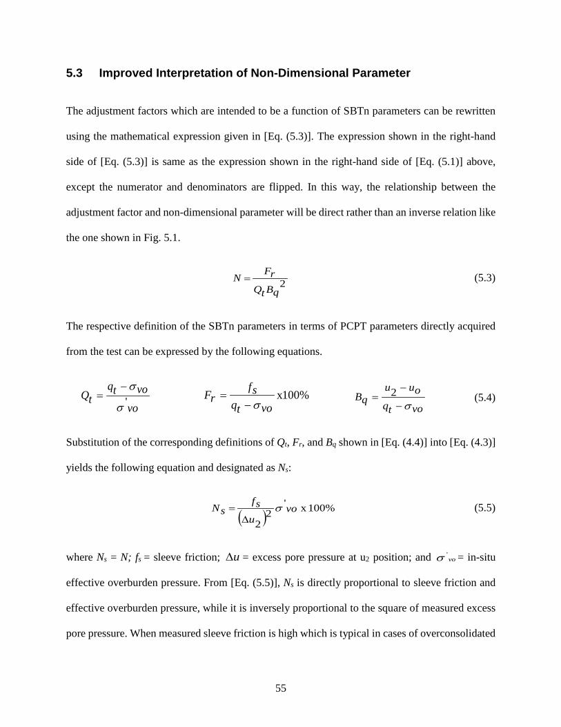
55

5.3 Improved Interpretation of Non-Dimensional Parameter

The adjustment factors which are intended to be a function of SBTn parameters can be rewritten

using the mathematical expression given in [Eq. (5.3)]. The expression shown in the right-hand

side of [Eq. (5.3)] is same as the expression shown in the right-hand side of [Eq. (5.1)] above,

except the numerator and denominators are flipped. In this way, the relationship between the

adjustment factor and non-dimensional parameter will be direct rather than an inverse relation like

the one shown in Fig. 5.1.

2 qBtQrF

N = (5.3)

The respective definition of the SBTn parameters in terms of PCPT parameters directly acquired

from the test can be expressed by the following equations.

vovotq

tQ 'σ

σ−= %100x

votqsf

rFσ−

= votqouu

qBσ−

−= 2 (5.4)

Substitution of the corresponding definitions of Qt, Fr, and Bq shown in [Eq. (4.4)] into [Eq. (4.3)]

yields the following equation and designated as Ns:

( )

100% x '2

2 vo

usf

sN σ∆

= (5.5)

where Ns = N; fs = sleeve friction; u∆ = excess pore pressure at u2 position; and vo'σ = in-situ

effective overburden pressure. From [Eq. (5.5)], Ns is directly proportional to sleeve friction and

effective overburden pressure, while it is inversely proportional to the square of measured excess

pore pressure. When measured sleeve friction is high which is typical in cases of overconsolidated

56

and cemented soils, the value of required adjustment factor will be higher too. Similarly, when

measured excess pore pressure is lower, a required adjustment factor value will be higher.

However, in literature, it is stated that sleeve friction is the less repeatable and reliable among

parameters obtained from PCPT (e.g. Lunne et al. 1986a). Thus, it was intended to substitute sleeve

friction in [Eq. (5.5)] by net cone tip resistance ( votq σ− ) as shown in [Eq. (5.6)].

( )( ) vo

votc u

qN '2

2

σσ∆−

= (4.6)

where Nc = modified N based on net cone tip resistance. The substitution of net cone tip resistance

yielded a parameter that resembles the factors that were used in (Campanella and Robertson 1981;

Tumay et al. 1982) for profiling OCR from PCPT except the inclusion of effective overburden

pressure and squaring of measured excess pore pressure to accommodate negative excess pore

pressures. Backward assembly of [Eq. (5.6)] into an equivalent expression in terms of piezocone

indices produced the equation shown below in [Eq. (5.7)]:

21

qtc BQ

N = (4.7)

[Eq. (5.7)] is similar in form to the non-dimensional parameter that was used in (Elsworth and Lee

2005) to estimate permeability of soils on-the-fly except Bq is squared in [Eq. (5.7)]. In subsequent

discussions, both Ns and Nc were used to estimate required correction factor C and relative accuracy

of these approaches in estimating hydraulic conductivity of overconsolidated soils was examined.

5.4 Results and Interpretation

Two sets of computed C and N based on PCPT data and oedometer data provided by NDOT were

plotted to determine the correlation that exists between C and N. Fig. 5.2 [a & b] show C versus N

plots on a full log scale for N computed based on [Eq. (5.5) and (5.6)] respectively.

57

(a) (b)

Fig. 5.2. Correlation between C and N (a) based on sleeve friction (b) based on cone resistance

From Fig. 5.2 (a) & (b), it is shown that the lower bound for the correction factor, C is around

unity, which indicates there is no need to apply correction to the measured excess pore pressure.

The relationship of C with Ns and Nc can be expressed by the following two equations:

38.080.1 sNC = (5.8)

45.038.2 cNC = (5.9)

The correlations express the relationship between C and Ns and Nc for about 84 % and 87 % of the

data set respectively, which can be considered as satisfactory. Once adjustment factors are obtained

on the fly using either [Eq. (5.8) or (5.9)], adjusted excess pore pressure can be estimated using

the following equation.

measureduCadjustedu ∆=∆ . (5.10)

58

Then, adjusted excess pore pressure from [Eq. (5.10)] can be introduced into the equation of Song

and Pulijala to give adjusted hydraulic conductivity. The modified Song and Pulijala equation after

the incorporation of adjusted excess pore pressure will have the following form.

0564.1

22.095,282

1)M,(

−∆

= adjustedadjusted

uf

k

κ

(5.11)

where adjustedk = adjusted hydraulic conductivity; adjustedu∆ = adjusted excess pore pressure. It

should be noted that measuredu∆ is obtained by subtracting the hydrostatic pore pressure from the

measured u2 pore pressure.

Fig. 5.3 shows computed hydraulic conductivity for six sites (project names are indicated in the

top right corner of each plot) using the modified (adjusted) and unmodified Song and Pulijala

equations. Laboratory determined κ and M = 1.20 are used to determine hydraulic conductivity

on the fly from the unmodified and modified equations. Dotted rectangular plots in this figure

show the range of hydraulic conductivity determined from oedometer test. Corrected hydraulic

conductivity profiles from modified Song and Pulijala equation show some cut off boundaries at

lower hydraulic conductivities. These boundaries are imposed in MS-Excel when adjustedu

f∆

)M,( κ ,which

is shown in [Eq. (4.11) above] is less than unity. This boundary hydraulic conductivity is 5 x 10-9

m/s which will designate the hydraulic conductivity of the soil is below it and cannot be

specifically stated.

59

60

Fig. 5.3 Hydraulic conductivity estimated from modified Song and Pulijala (2010)

Hydraulic conductivity estimated by applying adjustment factors based on sleeve friction (Ns) and

net cone tip resistance (Nc) have demonstrated similar patterns in Fig. 4.3. However, given the

non-repeatability of sleeve friction and better coefficient of determination for the C-Nc correlation,

correction factors determined from net cone tip resistance and excess pore pressure are more likely

reliable. Furthermore, supremacy of cone tip resistance based prediction of hydraulic conductivity

has been attested in some of the plots in Fig. 4.3. Therefore, following discussion will be restricted

to C-Nc correlations.

61

5.5 Verification with other Test data

Some sites from Korea, Canada, and the US are selected and the same equation used for the

prediction of hydraulic conductivity of overconsolidated soils in Nebraska is applied to PCPT data

collected at these sites to verify the applicability of the equation to soil profiles found outside

Nebraska.

5.5.1 Yangsan Mulgeum, Korea (Dong A Geology 1997)

This site is the old delta area of the Nakdong River. The soils are primarily young alluvial deposits.

The layers of this area’s profile starting from the surface consist of clayey and silty fill materials

followed by sedimentary layers consisting of clay, silty sand, silty clay, silt, sand, and gravel. Pore

pressure dissipation testing using PCPT shows the coefficient of consolidation is (2-6) ×10-7

m2/sec. Based on Robertson (2010), the projection of PCPT result of this site shows that the soil

is classified as silty clay to sandy silt with corresponding hydraulic conductivity ranging from 3 x

10-9 m/s to 1 x 10-5 m/s, as shown in Fig. 5.4(a). The ground water table is reported to be at a depth

of 1 m. From Fig. 5.4(a), the data points lean to the sensitive fine-grained soils. Some data points

are also inside the normally consolidated soils zone. In Fig. 5.4(b), the estimated hydraulic

conductivity shows good agreement with the measured hydraulic conductivity (indicated by the

rectangular dotted plot) at 15 m (50 ft.) below ground surface. Additionally, the estimated

hydraulic conductivity is slightly to the right (i.e. more permeable) of the measured hydraulic

conductivity. This can be considered reliable considering coefficient of consolidation from field

performance is generally larger than laboratory test results (Robertson et al. 1992); the difference

being a function of sensitivity and soil structure. Moreover, the uncorrected and adjusted

62

(corrected) hydraulic conductivity profiles are close to each other indicating the soil profile is

normally consolidated.

(a) (b)

Fig. 5.4. (a) SBTn classification (b) Estimated hydraulic property profile with depth for Yangsan Mulgeum, Korea (Data obtained from Dong A. Geology 1997)

5.5.2 Frazer River, Canada (Crawford and Campanella 1991)

The area is located about 25 km southeast of Vancouver on Highway 99. The surface of this area

is mostly flood plain, and the stratigraphy of the ground shows inter-bedded sand seams and peat

layers. The subsurface soils are relatively uniform with a natural water content of about 45% and

a liquid limit about 36%. From consolidation test results, the range of coefficients of

compressibility are 0.3-0.5, initial void ratios are 1.1-1.8, vertical coefficients of consolidation are

(0.6-2.8) × 10-7 m2/s, horizontal coefficients of consolidation are (0.7-7) × 10-7 m2/s, constrained

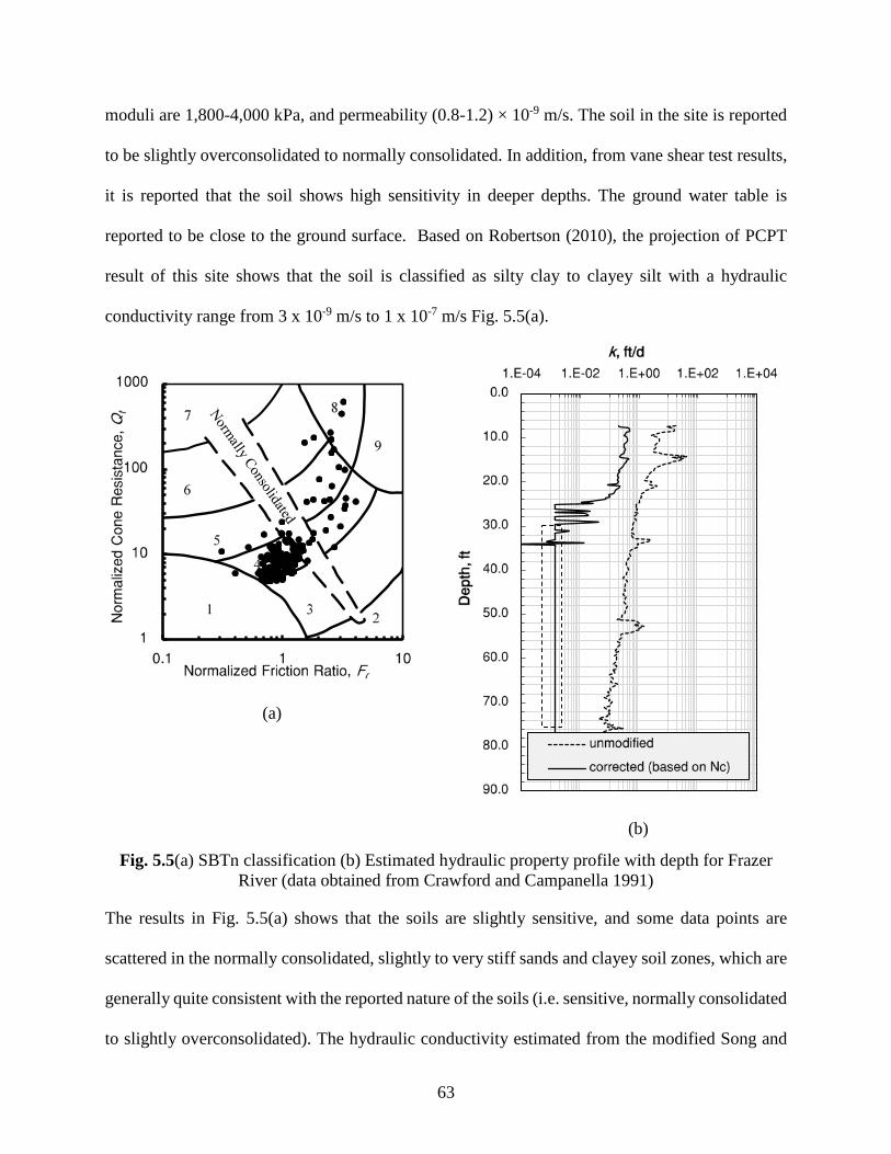
63

moduli are 1,800-4,000 kPa, and permeability (0.8-1.2) × 10-9 m/s. The soil in the site is reported

to be slightly overconsolidated to normally consolidated. In addition, from vane shear test results,

it is reported that the soil shows high sensitivity in deeper depths. The ground water table is

reported to be close to the ground surface. Based on Robertson (2010), the projection of PCPT

result of this site shows that the soil is classified as silty clay to clayey silt with a hydraulic

conductivity range from 3 x 10-9 m/s to 1 x 10-7 m/s Fig. 5.5(a).

(a)

(b)

Fig. 5.5(a) SBTn classification (b) Estimated hydraulic property profile with depth for Frazer River (data obtained from Crawford and Campanella 1991)

The results in Fig. 5.5(a) shows that the soils are slightly sensitive, and some data points are

scattered in the normally consolidated, slightly to very stiff sands and clayey soil zones, which are

generally quite consistent with the reported nature of the soils (i.e. sensitive, normally consolidated

to slightly overconsolidated). The hydraulic conductivity estimated from the modified Song and

64

Pulijala equation is quite close to the measured hydraulic conductivity (see Fig. 5.5(b)). Corrected

and uncorrected hydraulic conductivities are closer in the shallower depths, which might imply the

existence of normally consolidated soils, though there is significant deviation at deeper depths.

This might be due to increased sensitivity implying lower hydraulic conductivity as observed in

Robertson (2010). Moreover, corrected hydraulic conductivity ranges match those proposed by

Robertson (2010) for zone 4 soils.

5.5.3 Cheongna (Section 1), Incheon, Korea (Kaya Engineering Co. 2007)

This area consists of overconsolidated soil in the upper layer and normally consolidated soil in the

lower layer. Typical geotechnical properties show that the total unit weight is 1.57-1.95 t/m3, liquid

limit is 30-50%, natural water content is 20-40%, classification is CL, vertical coefficient of

consolidation is (1-10) × 10-7 m2/sec, horizontal coefficient of consolidation is (3-50) × 10-7 m2/sec,

coefficient of compressibility is 0.2-0.4, the depth of the soft layer is about 10 m, hydraulic

conductivity is (4.82- 89.6) x 10-8 m/s, and OCR is 0.62-5.50. The soil in this area primarily falls

under zones 3, 4, and 5. Data points in these zones are designated as clay to silty clay soils.

The hydraulic conductivity for these zones based on the SBTn chart ranges from 10-10 m/s to 10-7

m/s. Referring to Fig. 5.6(a), most of the data points are in the overconsolidated soils zones. The

scattered data points also show some layers are normally consolidated and somewhat sensitive.

Applying proper correction, the estimated hydraulic conductivity shows good agreement with the

reported hydraulic conductivity of this area at the depth shown by the dotted rectangular plot in

Fig. 5.6(b).

65

(a)

(b)

Fig. 5.6. (a) SBTn classification (b) Estimated hydraulic property profile with depth for Cheongna, Incheon, Korea (data obtained from Kaya Engineering Co. 2007)

5.5.4 SR 49, Indiana, USA (Kim 2005)

The area lies on the #49 road in Jasper County, Indiana. The normally consolidated clayey silty

layers exist up to 25 m deep from the ground surface, and the ground water table is located at a

level of 3 m below the surface. The average coefficient of consolidation evaluated from

consolidation tests was about 3.6×10-7 m2/sec. Fig. 5.7(b) shows adjusted and unadjusted

hydraulic conductivity plots. From the plot, estimated adjusted hydraulic conductivity is close to

measured hydraulic conductivity enclosed by the dotted rectangular plot. The projection of PCPT

result of this site into Robertson (2010) chart showed data points are scattered in the silty clay and

clayey silt zones which is consistent with reported classification of the soil. Range of hydraulic

66

conductivity estimated by (20) closely matches with measured hydraulic conductivity at 12.8 m

depth.

(a)

(b)

Fig. 5.7. (a) SBTn classification (b) Estimated hydraulic property profile with depth for SR 49, Indiana, USA (data obtained from Kim 2005)

67

6 PCPT DATA INTERPRETER USER GUIDE (VERSION 2) The newest version of the program adds several improvements and conveniences to the original

version. The previous version (in section 4.4) allows the user to extract information from PCPT

output data files, input site specific conditions (GWT, average assumed friction angle, and

recompression index), plot the hydraulic conductivity with depth according to this paper’s

correlation, and reset the form. The new version enables the user to change units between U.S. and

Metric, toggle the correlation to be based on either tip resistance or sleeve friction (where the tip

resistance correlation is typically more accurate), and export the chart to an excel sheet so that it

can be manipulated or transferred to reports. The exported chart can express the entire depth of the

data set on a single chart or break the data into up to four sections of 25 feet each (or meters if

metric units are selected). The new version also includes a button to open a user manual which is

built into the user form.

This program extracts the data output from piezocone penetration testing equipment and applies

appropriate adjustments to plot a continuous hydraulic conductivity profile versus depth. The

adjustments this program applies are consistent with those derived in this research concerning fast

estimation of hydraulic conductivity for overconsolidated soils using piezocone test results.

If macros have not previously been enabled on the computer’s installation of Excel, a security

warning will be displayed which states “Macros have been disabled,” with a button to the right

allowing the user to “Enable Content” (Fig. 6.1). This button must be pressed for the program to

begin. Alternatively, to avoid this step, the settings in Excel can be changed to allow macros to run

automatically on startup. This is done using the following path: File > Options > Trust Center >

Trust Center Settings > Macro Settings > Enable all macros. This is a global setting and will change

68

the settings of Excel as a whole, not just the PCPT program. This step is not necessary but

recommended for convenience. It is important to note that if macros are not automatically enabled,

the spreadsheet which normally runs in the background to execute necessary program functions

can be edited, which if done and saved will result in the program no longer operating correctly.

Fig. 6.1 Operating scree without macros enabled

The user form that is displayed on startup (Fig. 6.2) is the entire user interface for using the

program—the user will never interact directly with the excel sheet which runs in the background.

Once the user form appears on screen, “Select Data File” is clicked, which opens the PC’s file

69

explorer (Fig. 6.3) and allows for the selection of the piezocone’s output “.CSV” data sheet (with

columns A-D being H [m], qc [MPa], fs [MPa], and u2 [MPa], respectively, as shown in Fig. 6.4).

Fig. 6.2 User form on startup

Then, the user has the option to change the default values for GWT, friction angle, and

recompression index. After this, press “Plot” to see the hydraulic conductivity profile in the space

to the right. Fig. 6.5 shows the user form after plotting occurs. The reset function will tell the

70

program to no longer reference the previously selected data file and will erase the plot. Once this

is pressed, a new data file can be selected for analysis.

Fig. 6.3. File explorer to select PCPT data

The plot will by default show U.S. units of (ft/day) for k and (ft) for depth. This can be changed

by selecting the bubble next to “Metric” under the “Units” heading. Additionally, the graph can be

adjusted by changing the chosen correlation from tip resistance to sleeve friction The tip resistance

correlation is regarded as the more accurate of the two, but both are included so the user can

compare the two correlations found by this research.

The Export Chart button allows the user to save an excel sheet containing the plot shown on the

user form along with the data table from which the plot is comprised. This tool allows the user to

examine the computed hydraulic conductivity value for each depth that the piezocone took a

reading. Additionally, this is the button that should be used if the user wishes to copy the graph

into a report or print it. This graph can be edited the same way that graphs are typically edited in

Microsoft Excel. Fig. 6.6 shows an example output resulting from this feature. In addition to

71

displaying the graph of the entire depth of the testing data, intervals of 25 feet or meters can be

plotted to make report preparation easier.

Fig. 6.4 PCPT “.CSV” output columns A-D

If help is needed while using the program, the “User Manual” button can be pressed to provide an

abridged set of directions to help with operating the program. This is shown in Fig. 6.7.

72

Fig. 6.5 Plotted hydraulic conductivity profile on user form

73

Fig. 6.6 Excel sheet resulting from “Export Chart” button

Fig. 6.7 Built in user manual

74

7 CONCLUSION

The piezocone penetration testing device is known as one of the two more reliable geotechnical

testing devices. The built-in piezometer in the piezocone measures the pore pressure response

during penetration and used to profile soil layering systems. For saturated soils, this piezometer is

also used to conduct dissipation tests to obtain hydraulic conductivity or coefficient of

consolidation. A recent technique by Song and Pulijala (2010) eliminates the disadvantage of

dissipation tests and provided a more efficient way of determining hydraulic conductivity of soils.

The fundamental principle of this techniques is simultaneous generation and dissipation of pore

water pressure.

The main objective of this project was to estimate hydraulic conductivity of soils on a real time

basis using NDOT’s piezocone penetration test device. Further, focus was given to obtain

correction factors for measured pore pressure during PCPT. These correction factors were

necessitated as majority of Nebraskan soils are overconsolidated soils. Measured pore pressure in

overconsolidated soils are either negative or very small so that these factors will compensate

overconsolidation effects.

Correction factors were computed by matching up laboratory determined hydraulic conductivities

with PCPT based hydraulic conductivities obtained using Song and Pulijala’s equation. An attempt

was made to correlate the correction factors to SBTn chart parameters so that correction factors

can be obtained ‘on-the-fly’. The effect of sign of Bq was also investigated. It was found that the

sign of Bq has no significant influence on the correction factors. A correlation having a coefficient

of determination 86% between correction factor and non-dimensional parameter which is a

function of SBTn parameters Qt, Fr and Bq was obtained. The correlation was verified with

75

hydraulic conductivity and PCPT data from other test sites outside Nebraska and satisfactory

results has been obtained.

A VBA program to aid the determination hydraulic conductivity profile ‘on-the-fly’ was

developed. The program can be used as a standalone program to compute hydraulic conductivity

once PCPT data has been acquired.

References

Burns, S. and Mayne, P. (1998). Penetrometers for Soil Permeability and Chemical Detection. Georgia Institute of Technology, Atlanta.

Campanella, R.G., Robertson, P.K. (1981). "Applied cone research". Cone Penetration Testing

and Experience, ASCE, New York, 343-362.

Crawford, C. B., and R. G. Campanella. (1991). "Comparison of field consolidation with laboratory and in situ tests." Canadian Geotechnical Journal 103-112.

Dong A Geology. (1997). Piezocone testing report-settlement and stability control for constructing

Yangsan Mulgum Housing Complex. Dong A Geology Co.

Elsworth, D. (1993). Analysis of piezocone dissipation data using dislocation methods.” J. Geotech. Engrg., 119 (10), 1601–1623.

Elsworth, D. and Lee, D.S. (2005). “Permeability determination from on-the-fly piezocone

sounding.” J. Geotech. Geoenviron. Eng., 131 (5), 643–653. Houlsby, G.T. et al. (1988). Research at Oxford on the Analysis of the Piezocone Test, Oxford:

University of Oxford, Dept. of Eng. Science, U.K. Kaya Engineering Co. (2005). "Technical review of ground improvement techniques for

developing Chungra free trading area (District 1)". Kaya Engineering. Kim, K. (2005). "Cone penetration test in clayey soil: Rate effect and application to Pile Shaft

Resistance Calculations". Ph. D. Thesis, Purdue Univ. 218p.

Lee, Dae Sung, Derek Elsworth, and Roman Hryciw (2008). “Hydraulic Conductivity Measurement from On-The-Fly uCPT Sounding and from Viscpt”. Journal of Geotechnical and Geoenvironmental Engineering 134 (12), 1720-1729.

76

Levadoux, J. N., and Baligh, M. M. (1986). “Consolidation after undrained piezocone penetration. I: Prediction.” J. Geotech. Eng., 112 (7), 707–726.

Lunne, T., Eidsmoen, T., Gillespie, D., and Howland, J. (1986a). "Laboratory and field evaluation

of cone penetrometers". Use of In-Situ Tests in Geotechnical Engineering (GSP 6), ASCE,

New York, 714-729.

Lunne, T., Robertson, P. K., and Powell, J. J. M. (1997). Cone penetration testing in geotechnical practice, Blackie Academic & Professional, London, 48–71.

Manassero, M. (1994). "Hydraulic Conductivity Assessment of Slurry Wall using Piezocone Test" Robertson, P., & Cabal, K. (2010). Guide to Cone Penetration Testing . Signal Hill: Gregg Drilling

& Testing, Inc. Robertson, P., Sully, J., Woeller, D., Lunne, T., Powell, J., and Gillespie, D. (1992). "Estimating

coefficient of consolidation from piezocone tests". Canadian Geotech. J., 29(4), 539-550.

Rust, E., Jacobsz, S. and van der Berg P. (1995). "Seepage analysis from Piezocone dissipation

tests" Proceedings CPT’95, pp. 289-294.

Song, C. R. and S. Pulijala. (2010) “Hydraulic Property Estimation Using Piezocone Results”. Journal of Geotechnical and Geoenvironmental Engineering 136 (3): 456-463.

Song, C. R., Voyiadjis, G. Z., and Tumay, M. T. (1999). “Determination of permeability of soils

using multiple piezo-element penetrometer.” Int. J. Numer. Analyt. Meth. Geomech., 23 (13), 1609–1629.

Tumay, M.T., Acar, Y., deSeze, E., and Yimaz, R. (1982). "Soil exploration in soft clay with

electric cone penetrometer". Proc., 2nd European Symposium on Penetration Testing,

Amsterdam, 415-921.

Voyiadjis, G. Z., and Song, C. R. (2003). “Determination of hydraulic conductivity using piezocone penetration test.” Int. J. Geomech., 3(3/4), 217–224.

77

Appendix A

Table A.1 Summary of project identifications and amount of data

WT

Project # Total no. of bore holes General Location Station No. of lab

data points No. used

data points PCPT data WD IAD AD Remark

2-6(119) 3 S. Beltway road- Rod's outdoor power 159+32, 48' RT 5 4 Y N N N Used 160+47, 49' RT 5 3 Y N N N

161+70, 45' RT 5 4 Y N Y N 2-6(1027) 1 148th Street / N-2 12+50, 50' RT 6 6 Y N Y N Used 12-5(112) No BH log - - - - - - - - - 14-4(1016) 4 - - - - - - - - - 34-7(124) - La Platte, NE 5599+55, 248' RT - - N Y N N - 71-2(1005) No BH log I-80 to North of Kimball 765+70 CL - - Y N N N -

75-2(165) 3 Plattsmouth to Bellevue-Fairview 1112+00 CL 4 3 Y N Y N Used 7136+50, 20' RT 3 3 Y N Y N 75-2(176) 1 Chandler NB 224+90, 80' RT 3 2 Y N N N Used

75-2(1040) 9 Nebraska City South East 833+00, 150' RT 1 - Y N N N

Used 825+00, 50' LT 3 2 Y N Y N 821+20 CL 3 1 Y N Y N

75-2(1068) 5 Chandler Road NB 225+37, 166' RT 3 1 Y N N N Used 205+20, 160' RT 2 1 Y N N N

79-2(108) 2 Agnew North and South 623+90, 80' RT 1 1 Y N N Y Used 2 2 Y N N Y

80-9(829) 2 Church Road Over I-80 124+25, 25' LT 6 - Y N Y N Friction

was too small 126+30, 25' RT 3 - Y N Y N

80-9(837) 2 176th Street over I-80 4020+35, 20' RT 5 2 Y N N Y Used 4018+10, 40' LT 4 3 Y N N Y

80-9(839) 2 148th over I-80 119+70, 60' LT 5 5 Y N N Y Used 122+00, 30' LT 3 3 Y N N Y 80-9(849) 2 70th Street bridge-Lincoln 9010+59 RT 2 2 Y N Y N Used

78

WT

Project # Total no. of bore holes General Location Station No. of lab

data points No. used

data points PCPT data WD IAD AD Remark

9013+50 LT 1 1 Y N Y N 80-9(850) No BH log - - - - 80-9-(856) 1 I-180 to Hwy 77 6312+05, 30' RT 3 2 Y N N Y Used 80-9(862) 1 I-80 NW 56th to US 77 411+50, 115' LT 5 5 Y N N Y Used 80-9(889) - - - - - 80-9(1185) 1 Expand I80 WB, I80/480 Intercha 1295+86, 110' LT 7 6 Y N Y N Used

85-2(111) 3 Ralston viaduct 23+12, 83' LT 11 3 Y N N Y Used 21+75, 50' RT 6 3 Y N N Y

92-1(121) 2 Scottsbluff west viaduct 132+90, 58' RT 4 2 Y N N N Used 127+30, 62' RT 3 2 Y N Y N

183-3(112)

2 Ansley viaduct 1009+50, 5' RT 8 - Y N Y N Friction not

recorded 1013+75, 75' RT 6 - Y N Y N

281-3(110)

6 Greeley South 160+00 3 - Y N N N

- 231+00 3 - Y N N N 345+00, 20' RT 3 - Y N N Y 431+00 2 - Y N N N

Camera Tower - - - - - - - - 83-3(106) No BH log Thedford South - - - - - - - M2075A - - - - - - - -

L93E(1009) 1 Charleston Link 317+70, 15' RT 2 - Y N N N - N.B. Y-available, N-Not available, BH-Borehole

79

Appendix B

Table B.1 Hydraulic conductivity estimated based on laboratory test results

Project Depth Lab PCPT mv k k Cv eo Cc Cr σo σp OCR qt

m m2/s kPa kPa kPa 1/kPa m/s ft/d

2-6(119) RO-1

1.62 5.42E-06 0.65 0.19 0.03 27.94 504.58 18.06 2110.00 2.18E-05 1.18E-09 3.40E-04 2.34 6.85E-06 0.85 0.35 0.03 47.14 428.54 9.09 2161.00 3.42E-05 2.30E-09 6.63E-04 3.84 1.17E-05 0.76 0.38 0.04 68.26 449.28 6.58 1871.00 4.33E-05 4.95E-09 1.43E-03 5.96 7.38E-06 0.74 0.27 0.03 108.34 428.54 3.96 1631.00 3.37E-05 2.44E-09 7.03E-04 7.43 7.02E-06 0.45 0.11 0.02 134.88 331.68 2.46 2496.00 1.04E-05 7.17E-10 2.07E-04

2-6(119) RO-2

1.74 7.45E-06 0.61 0.14 0.02 31.39 297.22 9.47 3648.00 1.04E-05 7.72E-10 2.22E-04 3.84 8.80E-06 0.84 0.48 0.04 46.46 656.64 14.13 1930.00 5.87E-05 5.07E-09 1.46E-03 5.39 1.02E-05 0.79 0.40 0.04 74.40 656.64 8.83 1396.00 6.95E-05 6.93E-09 2.00E-03 6.00 1.85E-06 0.77 0.26 0.03 83.04 207.36 2.50 2232.00 3.05E-05 5.54E-10 1.60E-04 8.36 6.77E-07 0.37 0.09 0.02 132.34 525.31 3.97 3674.00 7.76E-06 5.15E-11 1.48E-05

2-6(119) RO-3

2.40 4.85E-06 0.74 0.31 0.03 46.18 387.07 8.38 1365.00 5.67E-05 2.70E-09 7.78E-04 3.84 1.08E-05 0.83 0.38 0.04 80.40 442.32 5.50 1262.00 7.15E-05 7.57E-09 2.18E-03 5.67 6.61E-07 0.99 0.41 0.03 102.00 248.88 2.44 754.00 1.19E-04 7.70E-10 2.22E-04 7.46 2.97E-07 0.41 0.01 0.03 145.20 511.49 3.52 3234.00 9.59E-07 2.79E-12 8.04E-07

2-6(1027)

1.50 2.92E-07 0.87 0.33 0.02 29.28 414.72 14.16 1142.00 6.71E-05 1.92E-10 5.53E-05 2.94 6.25E-07 0.80 0.25 0.03 42.72 168.00 3.93 703.00 8.58E-05 5.26E-10 1.51E-04 4.44 3.33E-07 1.03 0.41 0.03 55.01 103.68 1.88 818.00 1.07E-04 3.51E-10 1.01E-04 6.84 7.36E-06 0.66 0.25 0.02 79.30 511.44 6.45 1662.00 3.94E-05 2.84E-09 8.19E-04 8.94 1.28E-06 0.57 0.16 0.03 102.48 373.20 3.64 2102.00 2.11E-05 2.65E-10 7.63E-05 10.44 1.67E-06 0.54 0.14 0.03 118.70 622.08 5.24 2631.00 1.50E-05 2.45E-10 7.07E-05

75-2(165) PB-5 4.44 2.88E-06 0.88 0.38 0.03 80.64 311.04 3.86 756.00 1.16E-04 3.28E-09 9.43E-04 5.96 6.88E-07 0.99 0.44 0.02 108.67 200.45 1.84 457.00 2.10E-04 1.42E-09 4.08E-04 7.49 2.40E-07 0.95 0.24 0.02 136.90 136.92 1.00 837.00 6.39E-05 1.50E-10 4.33E-05

80

Project Depth Lab PCPT mv k k Cv eo Cc Cr σo σp OCR qt

75-2(165) W 5.96 3.44E-06 0.94 0.28 0.02 67.73 145.15 2.14 1200.00 5.23E-05 1.76E-09 5.07E-04 7.46 2.40E-06 1.09 0.28 0.02 78.53 165.89 2.11 470.00 1.24E-04 2.91E-09 8.38E-04 8.94 1.15E-05 1.00 0.32 0.03 90.58 241.92 2.67 900.00 7.72E-05 8.73E-09 2.51E-03

75-2(176) 4.35 1.21E-06 0.75 0.25 0.03 84.43 328.32 3.89 1496.00 4.14E-05 4.93E-10 1.42E-04 7.38 1.83E-06 0.71 0.24 0.01 134.78 490.75 3.64 769.00 7.93E-05 1.42E-09 4.09E-04 8.82 1.32E-06 0.70 0.21 0.02 173.04 248.88 1.44 832.00 6.44E-05 8.36E-10 2.41E-04

75-2(1040) NE-5 0.40 2.51E-06 0.73 0.21 0.02 10.56 311.04 29.45 1040.00 5.07E-05 1.25E-09 3.59E-04 2.36 7.24E-06 0.72 0.26 0.03 42.86 552.96 12.90 1800.00 3.64E-05 2.59E-09 7.45E-04 4.53 3.33E-07 0.55 0.21 0.03 66.96 456.00 6.81 2889.00 2.04E-05 6.66E-11 1.92E-05

75-2(1040) NE-6 0.85 1.35E-06 0.89 0.28 0.01 18.48 283.20 15.32 1032.00 6.23E-05 8.28E-10 2.38E-04 1.45 3.54E-06 0.81 0.42 0.02 29.86 656.64 21.99 910.00 1.11E-04 3.85E-09 1.11E-03 4.50 1.06E-05 0.66 0.22 0.03 76.56 518.40 6.77 3427.00 1.68E-05 1.75E-09 5.04E-04

75-2(1068) H10 7.56 8.58E-06 0.83 0.36 0.02 132.00 359.52 2.72 4009.00 2.13E-05 1.79E-09 5.17E-04 11.94 9.45E-06 0.61 0.19 0.03 217.68 552.96 2.54 3857.00 1.33E-05 1.23E-09 3.55E-04

79-2(108) SM-1 5.28 3.92E-07 1.01 0.22 0.02 90.00 90.00 1.00 1345.00 3.53E-05 1.36E-10 3.91E-05

79-2(108) SM-2 4.00 3.99E-08 1.16 0.31 0.06 68.64 165.84 2.42 406.00 1.53E-04 6.00E-11 1.73E-05 6.00 7.74E-08 1.10 0.35 0.09 86.30 172.80 2.00 607.00 1.19E-04 9.06E-11 2.61E-05

80-9(837) SM-1

0.81 3.48E-06 0.91 0.32 0.03 13.10 186.72 14.25 3220.00 2.26E-05 7.73E-10 2.22E-04 3.12 1.77E-06 0.77 0.31 0.02 53.04 359.04 6.77 3307.00 2.30E-05 4.00E-10 1.15E-04 4.50 5.98E-06 0.74 0.21 0.02 78.24 152.16 1.94 3132.00 1.67E-05 9.81E-10 2.82E-04 7.52 6.03E-06 0.74 0.23 0.03 135.60 518.40 3.82 2008.00 2.86E-05 1.69E-09 4.87E-04 10.50 1.36E-06 0.48 0.14 0.02 190.32 355.20 1.87 1127.00 3.65E-05 4.86E-10 1.40E-04

80-9(837) SM-2

1.53 2.96E-06 0.87 0.38 0.03 29.04 345.60 11.90 1370.00 6.45E-05 1.87E-09 5.39E-04 3.02 1.07E-05 0.82 0.30 0.02 54.72 283.20 5.18 1660.00 4.31E-05 4.53E-09 1.31E-03 4.64 3.66E-06 0.59 0.17 0.01 79.44 172.80 2.18 5038.00 9.21E-06 3.31E-10 9.53E-05 5.99 7.06E-06 0.71 0.28 0.03 111.84 345.60 3.09 1868.00 3.81E-05 2.63E-09 7.59E-04

80-9(839) 148-1 1.58 1.80E-06 0.74 0.24 0.03 31.92 324.48 10.17 2431.00 2.46E-05 4.35E-10 1.25E-04

81

Project Depth Lab PCPT mv k k Cv eo Cc Cr σo σp OCR qt

3.02 4.11E-06 0.76 0.27 0.02 59.76 193.44 3.24 1803.00 3.69E-05 1.49E-09 4.29E-04 4.61 7.21E-06 0.56 0.22 0.02 83.52 131.28 1.57 2456.00 2.49E-05 1.76E-09 5.08E-04 6.12 3.93E-06 0.56 0.16 0.02 112.08 414.72 3.70 2553.00 1.74E-05 6.73E-10 1.94E-04 8.97 1.35E-05 0.49 0.15 0.02 172.32 532.32 3.09 2916.00 1.50E-05 1.98E-09 5.72E-04

80-9(839) 148-2 4.00 4.86E-06 0.69 0.31 0.02 67.97 345.60 5.08 1734.00 4.60E-05 2.19E-09 6.31E-04 5.94 3.72E-06 0.70 0.21 0.02 114.48 228.00 1.99 3466.00 1.55E-05 5.64E-10 1.62E-04 8.97 1.22E-05 0.66 0.28 0.02 177.41 518.40 2.92 2190.00 3.35E-05 3.99E-09 1.15E-03

80-9(849) A1 0.89 8.56E-07 0.53 0.12 0.02 20.06 290.40 14.47 1526.00 2.23E-05 1.88E-10 5.41E-05 1.49 1.40E-07 0.53 0.11 0.02 32.74 483.84 14.78 2276.00 1.37E-05 1.88E-11 5.41E-06

80-9(849) A2 0.84 5.35E-07 0.62 0.08 0.02 28.42 324.72 11.43 970.00 2.21E-05 1.16E-10 3.33E-05

80-9(856) 1.52 2.10E-06 0.75 0.26 0.03 29.76 127.68 4.29 655.00 9.85E-05 2.03E-09 5.83E-04 3.09 5.79E-06 0.79 0.30 0.02 45.84 725.76 15.83 464.00 1.57E-04 8.91E-09 2.57E-03 7.43 9.81E-06 0.54 0.10 0.01 88.32 345.60 3.91 1910.00 1.48E-05 1.42E-09 4.09E-04

80-9(862) SM-1

1.56 1.15E-06 0.92 0.39 0.05 17.09 648.00 37.92 764.00 1.16E-04 1.32E-09 3.79E-04 2.94 4.11E-06 0.67 0.21 0.03 29.52 276.48 9.37 1965.00 2.82E-05 1.14E-09 3.28E-04 4.43 3.49E-06 0.60 0.34 0.05 43.49 449.28 10.33 1501.00 6.07E-05 2.08E-09 5.99E-04 4.73 4.82E-06 0.79 0.27 0.02 70.42 580.61 8.25 1365.00 4.84E-05 2.29E-09 6.59E-04 7.44 7.04E-06 0.97 0.24 0.02 83.71 622.08 7.43 1228.00 4.36E-05 3.01E-09 8.66E-04

80-9(1185)

1.47 2.07E-06 0.79 0.31 0.01 30.00 414.72 13.82 1027.00 7.23E-05 1.47E-09 4.23E-04 2.51 4.16E-06 0.72 0.26 0.02 44.06 366.34 8.31 1651.00 4.02E-05 1.64E-09 4.72E-04 2.99 3.15E-06 0.76 0.25 0.02 56.06 241.92 4.32 1172.00 5.20E-05 1.61E-09 4.62E-04 4.49 4.96E-06 0.69 0.25 0.02 90.48 449.28 4.97 1412.00 4.47E-05 2.17E-09 6.26E-04 5.99 7.08E-06 0.61 0.26 0.02 116.64 359.42 3.08 2763.00 2.53E-05 1.76E-09 5.06E-04 9.12 2.18E-06 0.78 0.18 0.02 176.02 235.01 1.34 2027.00 2.20E-05 4.70E-10 1.35E-04

85-2(111) H1 3.00 4.27E-08 0.86 0.49 0.03 54.48 54.48 1.00 409.00 2.79E-04 1.17E-10 3.37E-05 4.30 8.19E-07 0.68 0.24 0.02 74.59 100.80 1.35 850.00 7.20E-05 5.78E-10 1.67E-04 5.80 4.92E-07 1.08 0.25 0.02 103.44 115.44 1.12 883.00 5.81E-05 2.80E-10 8.07E-05

82

Project Depth Lab PCPT mv k k Cv eo Cc Cr σo σp OCR qt

7.45 2.43E-06 0.72 0.21 0.02 131.42 262.56 2.00 870.00 6.08E-05 1.45E-09 4.18E-04 8.77 9.80E-07 0.69 0.19 0.02 143.95 147.84 1.03 984.00 5.04E-05 4.85E-10 1.40E-04 10.28 7.99E-07 0.77 0.27 0.02 187.78 207.36 1.10 735.00 8.87E-05 6.95E-10 2.00E-04 16.28 1.02E-06 0.59 0.14 0.01 248.50 248.50 1.00 2884.00 1.29E-05 1.29E-10 3.70E-05

85-2(111) H3

2.42 2.07E-06 0.69 0.28 0.04 46.08 182.16 3.95 1014.00 7.10E-05 1.44E-09 4.14E-04 3.75 3.86E-07 0.86 0.27 0.04 67.92 219.36 3.23 469.00 1.33E-04 5.03E-10 1.45E-04 4.62 8.96E-07 0.84 0.25 0.03 87.60 147.84 1.69 499.00 1.18E-04 1.04E-09 2.98E-04 5.91 2.96E-06 0.90 0.26 0.04 104.16 126.48 1.21 562.00 1.04E-04 3.02E-09 8.69E-04 7.41 9.74E-07 1.03 0.45 0.04 117.36 230.16 1.96 663.00 1.44E-04 1.37E-09 3.96E-04 8.96 2.38E-06 0.85 0.29 0.04 130.56 167.28 1.28 729.00 9.41E-05 2.20E-09 6.32E-04

9-1(121) SW-1

1.66 3.10E-06 1.19 0.45 0.04 25.92 76.03 2.93 1478.00 6.04E-05 1.83E-09 5.28E-04 4.53 3.97E-07 1.17 0.51 0.02 71.38 89.86 1.26 1212.00 8.42E-05 3.28E-10 9.45E-05 6.00 9.36E-06 0.87 0.33 0.03 98.06 622.08 6.34 3134.00 2.44E-05 2.24E-09 6.46E-04 7.64 7.32E-06 1.89 0.19 0.01 125.18 359.42 2.87 913.00 3.13E-05 2.25E-09 6.48E-04

9-1(121) SW-2 4.62 5.97E-06 1.01 0.19 0.01 83.76 428.54 5.12 2954.00 1.39E-05 8.14E-10 2.35E-04 6.00 8.33E-06 0.98 0.33 0.02 104.45 642.82 6.15 3160.00 2.29E-05 1.87E-09 5.39E-04 7.60 1.04E-05 1.63 0.47 0.06 130.18 470.02 3.61 982.00 7.90E-05 8.09E-09 2.33E-03

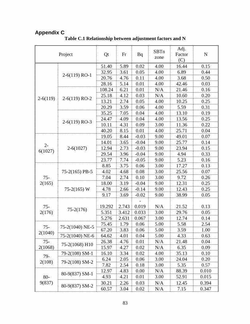
83

Appendix C Table C.1 Relationship between adjustment factors and N

Project Qt Fr Bq SBTn zone

Adj. Factor

(C) N

2-6(119)

2-6(119) RO-1

51.40 5.89 0.02 4.00 16.44 0.15 32.95 3.61 0.05 4.00 6.89 0.44 20.76 4.76 0.11 4.00 3.68 0.50 28.16 5.14 0.01 4.00 42.46 0.03

2-6(119) RO-2

108.24 6.21 0.01 N/A 21.46 0.16 25.18 4.12 0.03 N/A 10.60 0.20 13.21 2.74 0.05 4.00 10.25 0.25 20.29 3.59 0.06 4.00 5.59 0.31

2-6(119) RO-3

35.25 7.05 0.04 4.00 13.10 0.19 24.47 4.09 0.04 4.00 13.56 0.25 10.11 4.31 0.09 3.00 11.36 0.22 40.20 8.15 0.01 4.00 25.71 0.04

2-6(1027) 2-6(1027)

19.05 8.44 -0.03 9.00 49.01 0.07 14.01 3.65 -0.04 9.00 25.77 0.14 12.94 2.73 -0.03 9.00 23.94 0.15 29.54 3.96 -0.04 9.00 4.94 0.33 23.77 7.74 -0.05 9.00 5.23 0.16

75-2(165)

75-2(165) PB-5 8.85 3.75 0.06 3.00 17.27 0.13 4.02 4.68 0.08 3.00 25.56 0.07 7.04 2.74 0.10 3.00 9.72 0.26

75-2(165) W 18.00 3.19 -0.04 9.00 12.31 0.25 4.78 2.66 -0.14 9.00 12.43 0.25 9.17 3.69 -0.02 9.00 38.99 0.05

75-2(176) 75-2(176) 19.292 2.743

-0.019 N/A 21.52 0.13

5.351 3.412 0.033 3.00 29.76 0.05 5.276 2.631 0.067 3.00 12.74 0.14

75-2(1040)

75-2(1040) NE-5 75.45 1.79 0.06 5.00 5.58 2.54 67.20 3.83 0.06 5.00 3.59 1.00

75-2(1040) NE-6 64.62 4.01 0.04 5.00 4.33 0.63 75-

2(1068) 75-2(1068) H10 26.38 4.76 0.01 N/A 21.48 0.04 15.97 4.27 0.02 N/A 6.35 0.09

79-2(108)

79-2(108) SM-1 16.10 3.34 0.02 4.00 35.13 0.10

79-2(108) SM-2 6.24 2.05 0.06 3.00 24.04 0.20 7.82 2.54 0.18 3.00 5.35 0.57

80-9(837)

80-9(837) SM-1 12.97 4.83 0.00 N/A 88.39 0.010 4.93 4.21 0.01 3.00 52.91 0.015

80-9(837) SM-2 30.21 2.26 0.03 N/A 12.45 0.394 60.57 3.04 0.02 N/A 7.15 0.347

84

Project Qt Fr Bq SBTn zone

Adj. Factor

(C) N

15.93 5.47 0.01 N/A 26.19 0.038

80-9(839)

80-9(839) 148-1

79.97 8.54 0.00 N/A 285.05 0.01 30.63 3.35 0.04 N/A 9.82 0.32 27.63 8.26 0.00 N/A 97.45 0.01 21.15 6.00 0.01 N/A 21.59 0.04 17.19 4.41 0.04 4.00 6.23 0.14

80-9(839) 148-2 21.28 4.71 0.06 N/A 6.52 0.25 29.54 7.37 0.02 N/A 11.65 0.06 14.02 5.15 0.02 3.00 14.23 0.06

80-9(849)

80-9(849) A1 91.09 6.84 -0.03 N/A 12.83 0.44 80.63 3.82 -0.01 N/A 28.06 0.22

80-9(849) A2 63.49 8.31 -0.03 N/A 19.53 0.25 80-

9(856) 80-9(856) 33.84 3.50 0.11 4.00 3.44 1.02

80-9(862) 80-9(862) SM-1

64.86 2.07 0.03 5.00 9.08 1.04 35.43 3.43 0.09 4.00 4.28 0.90 30.33 3.87 0.10 4.00 4.57 0.79 17.31 1.75 -0.12 9.00 4.30 1.23

80-9(1185) 80-9(1185)

65.35 1.24 0.37 6.00 1.02 19.57 40.25 1.34 0.42 6.00 1.27 12.51 34.84 2.39 0.39 6.00 1.12 5.68 49.78 4.57 0.24 5.00 1.02 2.64 24.34 2.78 0.29 4.00 1.07 2.55

85-2(111)

85-2(111) H1

6.86 2.41 0.14 3.00 5.70 0.41 7.16 1.67 0.30 3.00 2.38 1.29 4.50 2.12 0.40 3.00 2.64 0.84 15.40 1.53 0.31 4.00 0.79 3.11

85-2(111) H3 5.54 1.28 0.15 3.00 7.80 0.65 5.89 1.46 0.28 3.00 3.64 1.11 5.73 1.87 0.33 3.00 2.83 1.02

9-1(121) 9-1(121) SW-1 34.14 8.92 0.01 4.00 16.45 0.04

7.53 7.02 0.05 3.00 15.20 0.06

9-1(121) SW-2 41.73 2.91 0.01 5.00 26.32 0.10 9.74 3.03 -0.05 9.00 13.11 0.15

85

Appendix D

Table D.1 Sample hydraulic conductivity computation based on PCPT

Project Name: - 2-6(119) RO-1 GWT

[ft] 6.66 M 1.2 κ 0.013

H [ft] qc [psi]

fs [psi] u [psi] qt [psi] Rf[%] UW

[kN/m3] u2[kPa] Uo

[kpa]

Exc. Pore [kPa] Δσv

σvo [kPa]

σvo' [kPa] Qt []

Fr [%] Bq [] Ic Zone Soil type

N C Uadj k (ft/d)

0.07 40.18 1.31 0.32 40.24 3.24 15.04 2.20 0.00 0.00 0.301 0.30 0.301 920.58 3.25 0.008 - - - 2.25 2.38 0.00 0.13 71.36 2.47 0.32 71.42 3.45 15.99 2.20 0.00 0.00 0.320 0.62 0.621 791.82 3.46 0.004 - - - 1.02 3.96 0.00 0.20 101.24 3.48 0.30 101.30 3.44 16.52 2.10 0.00 0.00 0.330 0.95 0.951 732.78 3.44 0.003 - - - 0.64 5.37 0.00 0.27 125.31 4.64 0.26 125.37 3.70 16.94 1.80 0.00 0.00 0.339 1.29 1.290 668.65 3.71 0.002 - - - 0.38 7.60 0.00 0.33 145.47 5.51 0.17 145.51 3.79 17.19 1.20 0.00 0.00 0.344 1.63 1.634 612.67 3.79 0.001 - - - 0.19 11.71 0.00 0.40 161.57 6.38 0.06 161.58 3.95 17.40 0.40 0.00 0.00 0.348 1.98 1.982 560.80 3.96 0.000 - - - 0.05 27.86 0.00 0.47 174.63 7.11 -0.07 174.61 4.07 17.55 -0.50 0.00 0.00 0.351 2.33 2.333 514.74 4.08 0.000 - - - 0.05 27.32 0.00 0.53 184.78 7.54 -0.20 184.74 4.08 17.64 -1.40 0.00 0.00 0.353 2.69 2.686 472.95 4.09 -0.001 - - - 0.13 15.37 0.00 0.60 192.61 7.98 -0.32 192.55 4.14 17.72 -2.20 0.00 0.00 0.354 3.04 3.040 435.39 4.15 -0.002 - - - 0.17 12.54 0.00 0.67 198.12 8.12 -0.42 198.04 4.10 17.75 -2.90 0.00 0.00 0.355 3.40 3.395 400.89 4.11 -0.002 - - - 0.21 11.18 0.00 0.73 201.75 8.27 -0.49 201.65 4.10 17.78 -3.40 0.00 0.00 0.356 3.75 3.751 369.42 4.11 -0.002 - - - 0.22 10.76 0.00 0.80 204.07 8.41 -0.54 203.96 4.12 17.81 -3.70 0.00 0.00 0.356 4.11 4.107 341.18 4.14 -0.003 - - - 0.22 10.84 0.00 0.87 205.23 8.41 -0.57 205.12 4.10 17.81 -3.90 0.00 0.00 0.356 4.46 4.463 315.65 4.11 -0.003 - - - 0.21 11.02 0.00 0.93 205.81 8.41 -0.58 205.69 4.09 17.81 -4.00 0.00 0.00 0.356 4.82 4.819 293.07 4.10 -0.003 - - - 0.20 11.38 0.00 1.00 206.10 8.41 -0.58 205.98 4.08 17.81 -4.00 0.00 0.00 0.356 5.18 5.175 273.22 4.10 -0.003 - - - 0.19 11.91 0.00 1.07 206.10 8.41 -0.58 205.98 4.08 17.81 -4.00 0.00 0.00 0.356 5.53 5.532 255.56 4.10 -0.003 - - - 0.18 12.44 0.00 1.13 206.10 8.56 -0.57 205.99 4.15 17.83 -3.90 0.00 0.00 0.357 5.89 5.888 240.03 4.17 -0.003 - - - 0.16 13.32 0.00 1.20 206.24 8.70 -0.52 206.14 4.22 17.85 -3.60 0.00 0.00 0.357 6.25 6.245 226.42 4.24 -0.003 - - - 0.14 14.73 0.00 1.27 206.53 8.85 -0.45 206.44 4.29 17.87 -3.10 0.00 0.00 0.357 6.60 6.603 214.43 4.31 -0.002 - - - 0.11 17.00 0.00 1.33 207.26 9.43 -0.33 207.19 4.55 17.94 -2.30 0.00 0.00 0.359 6.96 6.962 204.06 4.57 -0.002 - - - 0.07 22.22 0.00 1.40 208.27 10.01 -0.16 208.24 4.81 18.01 -1.10 0.00 0.00 0.360 7.32 7.322 194.96 4.83 -0.001 - - - 0.03 38.43 0.00 1.47 209.87 10.88 0.07 209.88 5.18 18.11 0.50 0.00 0.00 0.362 7.68 7.684 187.20 5.21 0.000 - - - 0.01 69.54 0.00 1.53 211.90 12.04 0.36 211.97 5.68 18.23 2.50 0.00 0.00 0.365 8.05 8.049 180.46 5.71 0.002 - - - 0.05 26.72 0.00 1.60 214.37 13.05 0.64 214.49 6.09 18.33 4.40 0.00 0.00 0.367 8.42 8.415 174.62 6.12 0.003 - - - 0.09 19.93 0.00 1.67 216.83 14.21 0.90 217.01 6.55 18.43 6.20 0.00 0.00 0.369 8.78 8.784 169.22 6.59 0.004 - - - 0.11 17.20 0.00 1.73 219.44 15.08 1.07 219.66 6.87 18.51 7.39 0.00 0.00 0.370 9.15 9.154 164.33 6.91 0.005 - - - 0.12 16.24 0.00 1.80 222.34 15.81 1.12 222.57 7.10 18.57 7.69 0.00 0.00 0.371 9.53 9.525 159.99 7.15 0.005 - - - 0.11 16.60 0.00 1.87 226.40 16.10 1.04 226.61 7.10 18.59 7.20 0.00 0.00 0.372 9.90 9.897 156.76 7.15 0.005 - - - 0.10 17.79 0.00 1.93 232.93 16.24 0.84 233.10 6.97 18.61 5.80 0.00 0.00 0.372 10.27 10.270 155.39 7.01 0.004 - - - 0.08 20.71 0.00 2.00 243.81 16.24 0.55 243.92 6.66 18.63 3.80 0.00 0.00 0.373 10.64 10.642 156.92 6.70 0.002 - - - 0.05 27.08 0.00 2.07 261.07 16.10 0.22 261.11 6.17 18.65 1.50 0.00 0.00 0.373 11.02 11.015 162.33 6.20 0.001 - - - 0.02 48.20 0.00 2.13 286.01 16.10 -0.09 286.00 5.63 18.68 -0.60 0.00 0.00 0.374 11.39 11.389 172.02 5.66 0.000 - - - 0.01 84.20 0.00 2.20 319.08 15.95 -0.36 319.01 5.00 18.71 -2.50 0.00 0.00 0.374 11.76 11.763 185.85 5.03 -0.001 - - - 0.04 31.48 0.00 2.27 359.40 16.10 -0.55 359.29 4.48 18.77 -3.80 0.00 0.00 0.375 12.14 12.139 202.94 4.50 -0.002 - - - 0.07 22.78 0.00 2.33 404.51 16.24 -0.68 404.37 4.02 18.83 -4.70 0.00 0.00 0.377 12.52 12.515 221.62 4.04 -0.002 - - - 0.09 18.85 0.00 2.40 451.07 16.53 -0.75 450.92 3.67 18.89 -5.20 0.00 0.00 0.378 12.89 12.893 239.97 3.68 -0.002 - - - 0.11 16.95 0.00

86

Project Name: - 2-6(119) RO-1 GWT

[ft] 6.66 M 1.2 κ 0.013

H [ft] qc [psi]

fs [psi] u [psi] qt [psi] Rf[%] UW

[kN/m3] u2[kPa] Uo

[kpa]

Exc. Pore [kPa] Δσv

σvo [kPa]

σvo' [kPa] Qt []

Fr [%] Bq [] Ic Zone Soil type

N C Uadj k (ft/d)

2.47 495.74 16.97 -0.80 495.58 3.42 18.95 -5.50 0.00 0.00 0.379 13.27 13.272 256.28 3.44 -0.002 - - - 0.12 15.93 0.00 2.53 534.90 17.55 -0.83 534.73 3.28 19.02 -5.70 0.00 0.00 0.380 13.65 13.652 268.87 3.29 -0.002 - - - 0.13 15.42 0.00 2.60 566.08 18.42 -0.87 565.91 3.25 19.10 -6.00 0.00 0.00 0.382 14.03 14.034 276.83 3.27 -0.002 - - - 0.13 15.10 0.00 2.67 587.84 19.44 -0.91 587.66 3.31 19.18 -6.30 0.00 0.00 0.384 14.42 14.418 279.83 3.32 -0.002 - - - 0.13 15.04 0.00 2.73 600.17 20.89 -0.97 599.97 3.48 19.27 -6.70 0.00 0.00 0.385 14.80 14.803 278.25 3.49 -0.002 - - - 0.13 15.20 0.00 2.80 603.65 22.48 -1.00 603.45 3.73 19.35 -6.90 0.00 0.00 0.387 15.19 15.190 272.71 3.74 -0.002 - - - 0.12 15.85 0.00 2.87 599.88 24.37 -1.02 599.67 4.06 19.44 -7.00 0.00 0.00 0.389 15.58 15.579 264.21 4.08 -0.002 - - - 0.11 16.89 0.00 2.93 590.59 26.54 -0.99 590.40 4.50 19.54 -6.80 0.00 0.00 0.391 15.97 15.970 253.72 4.51 -0.002 - - - 0.09 18.68 0.00 3.00 577.83 28.72 -0.93 577.65 4.97 19.62 -6.40 0.00 0.00 0.392 16.36 16.362 242.24 4.99 -0.002 - - - 0.08 21.08 0.00 3.07 563.47 30.89 -0.87 563.30 5.48 19.69 -6.00 0.00 0.00 0.394 16.76 16.756 230.63 5.51 -0.002 - - - 0.06 23.80 0.00 3.13 548.97 33.07 -0.83 548.80 6.03 19.76 -5.70 0.00 0.00 0.395 17.15 17.151 219.47 6.05 -0.002 - - - 0.05 26.56 0.00 3.20 535.77 34.95 -0.86 535.60 6.53 19.81 -5.90 0.00 0.00 0.396 17.55 17.547 209.30 6.56 -0.002 - - - 0.05 27.77 0.00 3.27 524.75 36.55 -0.99 524.55 6.97 19.86 -6.80 0.00 0.00 0.397 17.94 17.945 200.41 7.00 -0.002 - - - 0.05 26.81 0.00 3.33 516.63 37.85 -1.23 516.38 7.33 19.89 -8.49 0.00 0.00 0.398 18.34 18.342 192.97 7.37 -0.002 - - - 0.06 24.32 0.00 3.40 510.97 38.87 -1.61 510.65 7.61 19.92 -11.09 0.00 0.00 0.398 18.74 18.741 186.74 7.65 -0.003 - - - 0.08 21.25 0.00 3.47 507.63 39.60 -2.09 507.22 7.81 19.94 -14.39 0.00 0.00 0.399 19.14 19.139 181.59 7.85 -0.004 - - - 0.10 18.49 0.00 3.53 505.60 40.18 -2.61 505.08 7.95 19.95 -17.99 0.00 0.00 0.399 19.54 19.539 177.11 8.00 -0.005 - - - 0.12 16.41 0.00 3.60 503.72 40.47 -3.12 503.09 8.04 19.96 -21.49 0.00 0.00 0.399 19.94 19.938 172.86 8.09 -0.006 - - - 0.13 14.92 0.00 3.67 500.96 40.61 -3.55 500.25 8.12 19.96 -24.48 0.00 0.00 0.399 20.34 20.337 168.48 8.17 -0.007 - - - 0.15 13.97 0.00 3.73 496.76 40.76 -3.86 495.98 8.22 19.96 -26.58 0.00 0.00 0.399 20.74 20.736 163.80 8.27 -0.008 - - - 0.16 13.52 0.00 3.80 491.10 40.61 -4.03 490.29 8.28 19.95 -27.78 0.00 0.00 0.399 21.14 21.135 158.83 8.34 -0.008 - - - 0.16 13.37 0.00 3.87 484.28 40.47 -4.05 483.47 8.37 19.94 -27.88 0.00 0.00 0.399 21.53 21.534 153.69 8.42 -0.008 - - - 0.15 13.60 0.00 3.93 476.74 40.18 -3.95 475.95 8.44 19.93 -27.18 0.00 0.00 0.399 21.93 21.933 148.52 8.50 -0.008 - - - 0.15 14.07 0.00 4.00 469.34 39.89 -3.73 468.60 8.51 19.92 -25.68 0.00 0.00 0.398 22.33 22.331 143.58 8.57 -0.008 - - - 0.13 14.85 0.00 4.07 462.09 39.60 -3.45 461.40 8.58 19.90 -23.78 0.00 0.00 0.398 22.73 22.729 138.87 8.64 -0.008 - - - 0.12 15.88 0.00 4.13 455.27 39.31 -3.12 454.65 8.65 19.89 -21.49 0.00 0.00 0.398 23.13 23.127 134.45 8.71 -0.007 - - - 0.11 17.24 0.00 4.20 448.17 39.02 -2.77 447.61 8.72 19.87 -19.09 0.00 0.00 0.397 23.52 23.524 130.10 8.78 -0.006 - - - 0.09 18.93 0.00 4.27 440.63 38.73 -2.42 440.14 8.80 19.86 -16.69 0.00 0.00 0.397 23.92 23.921 125.77 8.87 -0.006 - - - 0.08 21.01 0.00 4.33 431.92 38.44 -2.09 431.51 8.91 19.84 -14.39 0.00 0.00 0.397 24.32 24.318 121.26 8.98 -0.005 - - - 0.07 23.58 0.00 4.40 422.35 38.00 -1.75 422.00 9.00 19.82 -12.09 0.00 0.00 0.396 24.71 24.715 116.65 9.08 -0.004 - - - 0.05 26.88 0.00 4.47 411.91 37.56 -1.45 411.62 9.13 19.80 -9.99 0.00 0.00 0.396 25.11 25.110 111.94 9.21 -0.004 - - - 0.04 31.01 0.00 4.53 400.89 36.84 -1.19 400.65 9.20 19.76 -8.19 0.00 0.00 0.395 25.51 25.506 107.23 9.28 -0.003 - - - 0.03 35.83 0.00 4.60 390.01 36.11 -0.94 389.82 9.26 19.73 -6.50 0.00 0.00 0.395 25.90 25.900 102.70 9.35 -0.002 - - - 0.03 42.30 0.00 4.67 379.56 35.24 -0.71 379.42 9.29 19.69 -4.90 0.00 0.00 0.394 26.29 26.294 98.42 9.38 -0.002 - - - 0.02 51.44 0.00 4.73 369.85 34.23 -0.51 369.75 9.26 19.65 -3.50 0.00 0.00 0.393 26.69 26.687 94.46 9.36 -0.001 - - - 0.01 64.51 0.00 4.80 361.14 33.36 -0.32 361.08 9.24 19.61 -2.20 0.00 0.00 0.392 27.08 27.079 90.87 9.34 -0.001 - - - 0.01 87.97 0.00 4.87 353.17 32.34 -0.13 353.14 9.16 19.57 -0.90 0.00 0.00 0.391 27.47 27.471 87.57 9.26 0.000 - - - 0.00 157.89 0.00 4.93 346.06 31.47 0.03 346.07 9.09 19.53 0.20 0.00 0.00 0.391 27.86 27.861 84.58 9.20 0.000 - - - 0.00 421.76 0.00 5.00 339.39 30.75 0.19 339.43 9.06 19.49 1.30 0.00 0.00 0.390 28.25 28.251 81.78 9.17 0.001 - - - 0.01 125.78 0.00 5.07 333.30 30.02 0.33 333.36 9.01 19.46 2.30 0.00 0.00 0.389 28.64 28.640 79.20 9.12 0.001 - - - 0.01 87.27 0.00 5.13 327.64 29.30 0.48 327.74 8.94 19.42 3.30 0.00 0.00 0.388 29.03 29.029 76.79 9.06 0.001 - - - 0.01 69.31 0.00 5.20 322.27 28.72 0.62 322.40 8.91 19.39 4.30 0.00 0.00 0.388 29.42 29.417 74.51 9.03 0.002 - - - 0.02 58.73 0.00

87

Project Name: - 2-6(119) RO-1 GWT

[ft] 6.66 M 1.2 κ 0.013

H [ft] qc [psi]

fs [psi] u [psi] qt [psi] Rf[%] UW

[kN/m3] u2[kPa] Uo

[kpa]

Exc. Pore [kPa] Δσv

σvo [kPa]

σvo' [kPa] Qt []

Fr [%] Bq [] Ic Zone Soil type

N C Uadj k (ft/d)

5.27 316.91 28.14 0.78 317.06 8.87 19.36 5.40 0.00 0.00 0.387 29.80 29.804 72.30 9.00 0.003 - - - 0.02 50.97 0.00 5.33 311.40 27.56 0.93 311.58 8.84 19.33 6.40 0.00 0.00 0.387 30.19 30.190 70.11 8.97 0.003 - - - 0.02 45.94 0.00 5.40 305.60 27.12 1.10 305.82 8.87 19.31 7.59 0.00 0.00 0.386 30.58 30.577 67.91 9.00 0.004 - - - 0.03 41.51 0.00 5.47 299.50 26.54 1.26 299.76 8.85 19.28 8.69 0.00 0.00 0.386 30.96 30.962 65.70 8.99 0.004 - - - 0.03 38.30 0.00 5.53 292.98 26.11 1.44 293.26 8.90 19.25 9.89 0.00 0.00 0.385 31.35 31.347 63.46 9.04 0.005 - - - 0.03 35.64 0.00 5.60 286.45 25.67 1.61 286.77 8.95 19.22 11.09 0.00 0.00 0.384 31.73 31.732 61.27 9.10 0.006 - - - 0.04 33.48 0.00 5.67 280.21 25.09 1.77 280.57 8.94 19.19 12.19 0.00 0.00 0.384 32.12 32.115 59.19 9.09 0.006 - - - 0.04 31.72 0.00 5.73 274.41 24.66 1.93 274.80 8.97 19.16 13.29 0.00 0.00 0.383 32.50 32.498 57.26 9.13 0.007 - - - 0.04 30.30 0.00 5.80 269.63 24.08 2.07 270.04 8.92 19.12 14.29 0.00 0.00 0.382 32.88 32.881 55.59 9.08 0.008 - - - 0.05 29.02 0.00 5.87 266.14 23.64 2.20 266.59 8.87 19.10 15.19 0.00 0.00 0.382 33.26 33.263 54.22 9.03 0.008 - - - 0.05 28.01 0.00 5.93 264.11 23.06 2.34 264.58 8.72 19.07 16.09 0.00 0.00 0.381 33.64 33.644 53.18 8.88 0.009 - - - 0.05 26.88 0.00 6.00 263.82 22.63 2.47 264.32 8.56 19.04 16.99 0.00 0.00 0.381 34.02 34.025 52.52 8.72 0.010 - - - 0.06 25.84 0.00 6.07 264.98 22.34 2.60 265.50 8.41 19.03 17.89 0.00 0.00 0.381 34.41 34.406 52.17 8.57 0.010 - - - 0.06 24.89 0.00 6.13 267.60 22.05 2.74 268.14 8.22 19.02 18.89 0.00 0.00 0.380 34.79 34.786 52.11 8.38 0.010 - - - 0.06 23.84 0.00 6.20 271.08 21.76 2.89 271.65 8.01 19.01 19.89 0.00 0.00 0.380 35.17 35.166 52.22 8.16 0.011 - - - 0.07 22.82 0.00 6.27 275.28 21.61 3.06 275.89 7.83 19.01 21.09 0.00 0.00 0.380 35.55 35.546 52.48 7.98 0.011 - - - 0.07 21.81 0.00 6.33 280.07 21.47 3.23 280.72 7.65 19.01 22.28 0.00 0.00 0.380 35.93 35.926 52.84 7.79 0.012 - - - 0.08 20.85 0.00 6.40 285.29 21.47 3.42 285.97 7.51 19.01 23.58 0.00 0.00 0.380 36.31 36.307 53.27 7.65 0.012 - - - 0.08 19.99 0.00 6.47 291.24 21.32 3.63 291.96 7.30 19.01 24.98 0.00 0.00 0.380 36.69 36.687 53.83 7.44 0.013 - - - 0.09 19.04 0.00 6.53 297.91 21.32 3.81 298.67 7.14 19.02 26.28 0.00 0.00 0.380 37.07 37.067 54.52 7.27 0.013 - - - 0.10 18.27 0.00 6.60 305.45 21.32 3.99 306.25 6.96 19.03 27.48 0.00 0.00 0.381 37.45 37.448 55.35 7.09 0.013 - - - 0.10 17.58 0.00 6.67 314.15 21.47 4.15 314.98 6.81 19.05 28.58 0.02 28.56 0.381 37.83 37.809 56.40 6.94 0.013 2.7 4.000 clayey silt to silty clay 0.11 17.01 485.78 1.21E-01 6.73 323.43 21.47 4.29 324.29 6.62 19.06 29.58 0.22 29.36 0.381 38.21 37.995 57.80 6.73 0.013 2.7 4.000 clayey silt to silty clay 0.11 16.44 482.74 1.25E-01 6.80 332.86 21.61 4.41 333.74 6.48 19.08 30.38 0.41 29.97 0.382 38.59 38.180 59.22 6.59 0.013 2.7 4.000 clayey silt to silty clay 0.12 16.04 480.70 1.27E-01 6.87 341.71 21.76 4.51 342.61 6.35 19.10 31.08 0.61 30.47 0.382 38.97 38.366 60.51 6.46 0.013 2.6 4.000 clayey silt to silty clay 0.12 15.71 478.84 1.30E-01 6.93 348.96 22.05 4.58 349.88 6.30 19.12 31.58 0.80 30.77 0.382 39.36 38.552 61.51 6.41 0.013 2.6 4.000 clayey silt to silty clay 0.12 15.58 479.54 1.29E-01 7.00 354.04 22.34 4.64 354.97 6.29 19.14 31.98 1.00 30.98 0.383 39.74 38.739 62.11 6.40 0.013 2.6 4.000 clayey silt to silty clay 0.13 15.55 481.71 1.26E-01 7.07 356.36 22.63 4.70 357.30 6.33 19.16 32.38 1.20 31.18 0.383 40.12 38.926 62.21 6.44 0.013 2.6 4.000 clayey silt to silty clay 0.12 15.60 486.35 1.20E-01 7.13 355.78 22.92 4.77 356.73 6.42 19.17 32.88 1.39 31.48 0.383 40.51 39.113 61.81 6.53 0.013 2.6 4.000 clayey silt to silty clay 0.12 15.70 494.16 1.10E-01 7.20 353.02 23.35 4.84 353.99 6.60 19.19 33.38 1.59 31.79 0.384 40.89 39.301 61.02 6.71 0.013 2.7 4.000 clayey silt to silty clay 0.12 15.92 506.11 9.61E-02 7.27 348.38 23.50 4.93 349.37 6.73 19.19 33.98 1.79 32.19 0.384 41.27 39.488 59.91 6.84 0.014 2.7 4.000 clayey silt to silty clay 0.12 16.04 516.51 8.43E-02 7.33 342.72 23.50 5.03 343.73 6.84 19.19 34.68 1.98 32.69 0.384 41.66 39.676 58.64 6.96 0.014 2.7 4.000 clayey silt to silty clay 0.12 16.11 526.61 7.34E-02 7.40 337.07 23.35 5.16 338.10 6.91 19.17 35.58 2.18 33.40 0.383 42.04 39.863 57.38 7.03 0.015 2.7 4.000 clayey silt to silty clay 0.12 16.05 535.92 6.37E-02 7.47 331.56 22.77 5.28 332.61 6.85 19.14 36.37 2.37 34.00 0.383 42.42 40.050 56.16 6.98 0.015 2.7 4.000 clayey silt to silty clay 0.12 15.82 538.01 6.16E-02 7.53 326.92 22.05 5.40 327.99 6.72 19.10 37.17 2.57 34.60 0.382 42.81 40.236 55.10 6.85 0.016 2.7 4.000 clayey silt to silty clay 0.13 15.51 536.67 6.30E-02 7.60 322.71 21.18 5.50 323.81 6.54 19.05 37.87 2.77 35.11 0.381 43.19 40.420 54.13 6.67 0.016 2.7 4.000 clayey silt to silty clay 0.13 15.14 531.58 6.82E-02 7.67 318.79 20.16 5.60 319.91 6.30 18.98 38.57 2.96 35.61 0.380 43.57 40.604 53.21 6.43 0.016 2.7 4.000 clayey silt to silty clay 0.14 14.69 523.21 7.70E-02 7.73 315.02 19.00 5.70 316.16 6.01 18.91 39.27 3.16 36.11 0.378 43.94 40.786 52.33 6.13 0.017 2.7 4.000 clayey silt to silty clay 0.14 14.16 511.43 9.00E-02 7.80 310.82 17.98 5.83 311.98 5.76 18.84 40.17 3.35 36.82 0.377 44.32 40.967 51.39 5.89 0.017 2.7 4.000 clayey silt to silty clay 0.15 13.65 502.75 1.00E-01 7.87 306.32 16.97 5.98 307.52 5.52 18.77 41.17 3.55 37.62 0.375 44.70 41.146 50.41 5.64 0.018 2.6 4.000 clayey silt to silty clay 0.16 13.13 493.93 1.11E-01 7.93 301.53 16.10 6.16 302.77 5.32 18.70 42.47 3.75 38.72 0.374 45.07 41.324 49.39 5.43 0.019 2.6 4.000 clayey silt to silty clay 0.17 12.62 488.61 1.17E-01 8.00 296.46 15.23 6.37 297.73 5.12 18.63 43.87 3.94 39.93 0.373 45.44 41.500 48.33 5.23 0.020 2.6 4.000 clayey silt to silty clay 0.18 12.10 483.08 1.24E-01

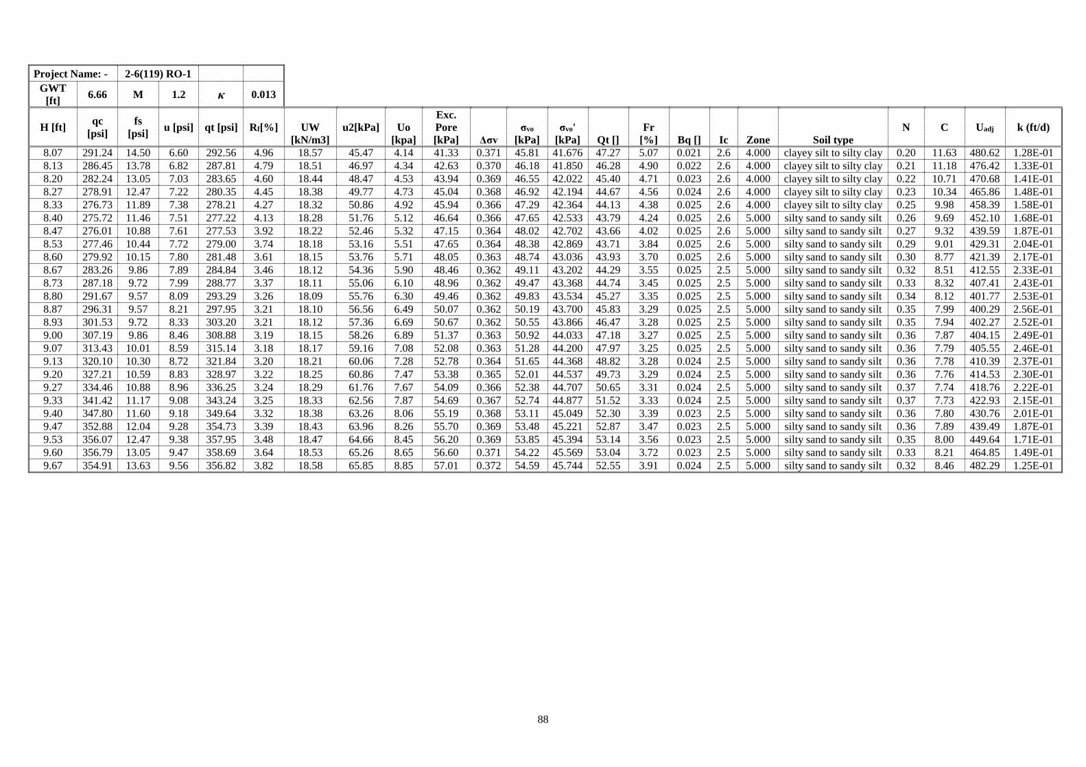
88

Project Name: - 2-6(119) RO-1 GWT

[ft] 6.66 M 1.2 κ 0.013

H [ft] qc [psi]

fs [psi] u [psi] qt [psi] Rf[%] UW

[kN/m3] u2[kPa] Uo

[kpa]

Exc. Pore [kPa] Δσv

σvo [kPa]

σvo' [kPa] Qt []

Fr [%] Bq [] Ic Zone Soil type

N C Uadj k (ft/d)

8.07 291.24 14.50 6.60 292.56 4.96 18.57 45.47 4.14 41.33 0.371 45.81 41.676 47.27 5.07 0.021 2.6 4.000 clayey silt to silty clay 0.20 11.63 480.62 1.28E-01 8.13 286.45 13.78 6.82 287.81 4.79 18.51 46.97 4.34 42.63 0.370 46.18 41.850 46.28 4.90 0.022 2.6 4.000 clayey silt to silty clay 0.21 11.18 476.42 1.33E-01 8.20 282.24 13.05 7.03 283.65 4.60 18.44 48.47 4.53 43.94 0.369 46.55 42.022 45.40 4.71 0.023 2.6 4.000 clayey silt to silty clay 0.22 10.71 470.68 1.41E-01 8.27 278.91 12.47 7.22 280.35 4.45 18.38 49.77 4.73 45.04 0.368 46.92 42.194 44.67 4.56 0.024 2.6 4.000 clayey silt to silty clay 0.23 10.34 465.86 1.48E-01 8.33 276.73 11.89 7.38 278.21 4.27 18.32 50.86 4.92 45.94 0.366 47.29 42.364 44.13 4.38 0.025 2.6 4.000 clayey silt to silty clay 0.25 9.98 458.39 1.58E-01 8.40 275.72 11.46 7.51 277.22 4.13 18.28 51.76 5.12 46.64 0.366 47.65 42.533 43.79 4.24 0.025 2.6 5.000 silty sand to sandy silt 0.26 9.69 452.10 1.68E-01 8.47 276.01 10.88 7.61 277.53 3.92 18.22 52.46 5.32 47.15 0.364 48.02 42.702 43.66 4.02 0.025 2.6 5.000 silty sand to sandy silt 0.27 9.32 439.59 1.87E-01 8.53 277.46 10.44 7.72 279.00 3.74 18.18 53.16 5.51 47.65 0.364 48.38 42.869 43.71 3.84 0.025 2.6 5.000 silty sand to sandy silt 0.29 9.01 429.31 2.04E-01 8.60 279.92 10.15 7.80 281.48 3.61 18.15 53.76 5.71 48.05 0.363 48.74 43.036 43.93 3.70 0.025 2.6 5.000 silty sand to sandy silt 0.30 8.77 421.39 2.17E-01 8.67 283.26 9.86 7.89 284.84 3.46 18.12 54.36 5.90 48.46 0.362 49.11 43.202 44.29 3.55 0.025 2.5 5.000 silty sand to sandy silt 0.32 8.51 412.55 2.33E-01 8.73 287.18 9.72 7.99 288.77 3.37 18.11 55.06 6.10 48.96 0.362 49.47 43.368 44.74 3.45 0.025 2.5 5.000 silty sand to sandy silt 0.33 8.32 407.41 2.43E-01 8.80 291.67 9.57 8.09 293.29 3.26 18.09 55.76 6.30 49.46 0.362 49.83 43.534 45.27 3.35 0.025 2.5 5.000 silty sand to sandy silt 0.34 8.12 401.77 2.53E-01 8.87 296.31 9.57 8.21 297.95 3.21 18.10 56.56 6.49 50.07 0.362 50.19 43.700 45.83 3.29 0.025 2.5 5.000 silty sand to sandy silt 0.35 7.99 400.29 2.56E-01 8.93 301.53 9.72 8.33 303.20 3.21 18.12 57.36 6.69 50.67 0.362 50.55 43.866 46.47 3.28 0.025 2.5 5.000 silty sand to sandy silt 0.35 7.94 402.27 2.52E-01 9.00 307.19 9.86 8.46 308.88 3.19 18.15 58.26 6.89 51.37 0.363 50.92 44.033 47.18 3.27 0.025 2.5 5.000 silty sand to sandy silt 0.36 7.87 404.15 2.49E-01 9.07 313.43 10.01 8.59 315.14 3.18 18.17 59.16 7.08 52.08 0.363 51.28 44.200 47.97 3.25 0.025 2.5 5.000 silty sand to sandy silt 0.36 7.79 405.55 2.46E-01 9.13 320.10 10.30 8.72 321.84 3.20 18.21 60.06 7.28 52.78 0.364 51.65 44.368 48.82 3.28 0.024 2.5 5.000 silty sand to sandy silt 0.36 7.78 410.39 2.37E-01 9.20 327.21 10.59 8.83 328.97 3.22 18.25 60.86 7.47 53.38 0.365 52.01 44.537 49.73 3.29 0.024 2.5 5.000 silty sand to sandy silt 0.36 7.76 414.53 2.30E-01 9.27 334.46 10.88 8.96 336.25 3.24 18.29 61.76 7.67 54.09 0.366 52.38 44.707 50.65 3.31 0.024 2.5 5.000 silty sand to sandy silt 0.37 7.74 418.76 2.22E-01 9.33 341.42 11.17 9.08 343.24 3.25 18.33 62.56 7.87 54.69 0.367 52.74 44.877 51.52 3.33 0.024 2.5 5.000 silty sand to sandy silt 0.37 7.73 422.93 2.15E-01 9.40 347.80 11.60 9.18 349.64 3.32 18.38 63.26 8.06 55.19 0.368 53.11 45.049 52.30 3.39 0.023 2.5 5.000 silty sand to sandy silt 0.36 7.80 430.76 2.01E-01 9.47 352.88 12.04 9.28 354.73 3.39 18.43 63.96 8.26 55.70 0.369 53.48 45.221 52.87 3.47 0.023 2.5 5.000 silty sand to sandy silt 0.36 7.89 439.49 1.87E-01 9.53 356.07 12.47 9.38 357.95 3.48 18.47 64.66 8.45 56.20 0.369 53.85 45.394 53.14 3.56 0.023 2.5 5.000 silty sand to sandy silt 0.35 8.00 449.64 1.71E-01 9.60 356.79 13.05 9.47 358.69 3.64 18.53 65.26 8.65 56.60 0.371 54.22 45.569 53.04 3.72 0.023 2.5 5.000 silty sand to sandy silt 0.33 8.21 464.85 1.49E-01 9.67 354.91 13.63 9.56 356.82 3.82 18.58 65.85 8.85 57.01 0.372 54.59 45.744 52.55 3.91 0.024 2.5 5.000 silty sand to sandy silt 0.32 8.46 482.29 1.25E-01