
Pierre-Louis Curien- Introduction to linear logic and ludics, Part II
49
a r X i v : c s / 0 5 0 1 0 3 9 v 1 [ c s . L O ] 1 9 J a n 2 0 0 5 Introduction to linear logic and ludics, Part II Pierre-Louis Curien (CNRS & Un iversit´ e Paris VII) ∗ February 1, 2008 Abstract This paper is the second part of an introduction to linear logic and ludics, both due to Girard. It is devoted to proof nets, in the limited, yet central, framework of multiplicative linear logic (section 1) and to ludics, which has been recently developped in an aim of further unveiling the fundamental interactive nature of computation and logic (sections 2, 3, 4, and 5). We hope to offer a few computer science insights into this new theory. Keywords : Cut-e limina tion (03F05), Linear logic (03F52), Logic in comp uter science (03B70) , In- teractive modes of computation (68Q10), Semantics (68Q55), Programming languages (68N15). Prerequisites This part depends mostly on the first two sections of part I, and should therefore be accessible to any one who has been exposed to the very first steps of linear logic. We have used the following sources: [29, 23, 38] for proof nets, and and [35, 36] for ludics. 1 Proof nets Proof nets are graphs that give a more economical presentation of proofs, abstracting from some irrelevant order of application of the rules of linear logic given in sequent calculus style (sections 2 and 3 of part I). We limit ourselves here to multiplicative linear logic (MLL), and we shall even begin with cut-fr ee MLL. Proof nets for MLL are graphs which are “almost tree s”, and we stress this by our choice of prese ntation. We invit e the reader to draw proof nets by himse lf while reading the sect ion. What plays here the role of a proof of a sequent ⊢ A 1 ,...,A n is the forest of the formulas A 1 ,...,A n represented as trees, together with a partition of the leaves of the forest in pairs (corresponding to the application of an axiom ⊢ C, C ⊥ ). Well, not quite. A proo f may not decompose eac h formula completely, since an axiom ⊢ C, C ⊥ can be applied to any formula. Hence we hav e to specify partial trees for the formulas A 1 ,...,A n . One wa y to do this is to specify the set of lea ve s of eac h parti al tree as a set of (pairwise disjoint) occurrences. F ormall y , an occurre nce is a word ove r {1, 2}, and the subformula A/u at occurrence u is defined by the following formal system: A/ǫ = A (A 1 ⊗ A 2 )/1u = (A 1 A 2 )/1u = A 1 /u (A 1 ⊗ A 2 )/2u = (A 1 A 2 )/2u = A 2 /u . ∗ Laboratoire Preuves, Pro grammes et Syst` emes, Cas e 7014, 2 pla ce Jus sie u, 75251 Pa ris Cede x 05, France, [email protected]. 1
Transcript of Pierre-Louis Curien- Introduction to linear logic and ludics, Part II

8/3/2019 Pierre-Louis Curien- Introduction to linear logic and ludics, Part II
http://slidepdf.com/reader/full/pierre-louis-curien-introduction-to-linear-logic-and-ludics-part-ii 1/49
a r X i v : c s / 0 5 0 1 0 3 9 v 1
[ c s . L O ]
1 9 J a n 2 0 0 5
Introduction to linear logic and ludics, Part II
Pierre-Louis Curien (CNRS & Universite Paris VII)∗
February 1, 2008
Abstract
This paper is the second part of an introduction to linear logic and ludics, both due to Girard.It is devoted to proof nets, in the limited, yet central, framework of multiplicative linear logic(section 1) and to ludics, which has been recently developped in an aim of further unveiling thefundamental interactive nature of computation and logic (sections 2, 3, 4, and 5). We hope tooffer a few computer science insights into this new theory.
Keywords: Cut-elimination (03F05), Linear logic (03F52), Logic in computer science (03B70), In-teractive modes of computation (68Q10), Semantics (68Q55), Programming languages (68N15).
Prerequisites
This part depends mostly on the first two sections of part I, and should therefore be accessible to anyone who has been exposed to the very first steps of linear logic. We have used the following sources:[29, 23, 38] for proof nets, and and [35, 36] for ludics.
1 Proof nets
Proof nets are graphs that give a more economical presentation of proofs, abstracting from someirrelevant order of application of the rules of linear logic given in sequent calculus style (sections 2and 3 of part I). We limit ourselves here to multiplicative linear logic (MLL), and we shall even beginwith cut-free MLL. Proof nets for MLL are graphs which are “almost trees”, and we stress this by ourchoice of presentation. We invite the reader to draw proof nets by himself while reading the section.
What plays here the role of a proof of a sequent ⊢ A1, . . . , An is the forest of the formulas A1, . . . , An
represented as trees, together with a partition of the leaves of the forest in pairs (corresponding tothe application of an axiom ⊢ C, C ⊥). Well, not quite. A proof may not decompose each formulacompletely, since an axiom ⊢ C, C ⊥ can be applied to any formula. Hence we have to specify partialtrees for the formulas A1, . . . , An. One way to do this is to specify the set of leaves of each partial
tree as a set of (pairwise disjoint) occurrences. Formally, an occurrence is a word over 1, 2, and thesubformula A/u at occurrence u is defined by the following formal system:
A/ǫ = A (A1 ⊗ A2)/1u = (A1A2)/1u = A1/u (A1 ⊗ A2)/2u = (A1A2)/2u = A2/u .∗Laboratoire Preuves, Programmes et Systemes, Case 7014, 2 place Jussieu, 75251 Paris Cedex 05, France,
1

8/3/2019 Pierre-Louis Curien- Introduction to linear logic and ludics, Part II
http://slidepdf.com/reader/full/pierre-louis-curien-introduction-to-linear-logic-and-ludics-part-ii 2/49
A partial formula tree AU consists of a formula A together with a set U of pairwise disjoint occurrencessuch that (∀ u ∈ U A/u is defined). Recall that a partition of a set E is a set X of non-empty subsets
of E which are pairwise disjoint and whose union is E . If X = Y 1, . . . , Y n we often simply writeX = Y 1, . . . , Y n.
Definition 1.1 A proof structure is given by
AU 11 , . . . , AU n
n [X ] ,
where AU 11 , . . . , AU n
n is a multiset of partial formula trees and where X is a partition of A1/u |u ∈ U 1 ∪ . . . ∪ An/u | u ∈ U n (disjoint union) whose classes are pairs of dual formulas. We shallsay that each class of the partition is an axiom of the proof structure, and that A1, . . . , An are theconclusions of the proof structure.
More generally, we shall manipulate graphs described as a forest plus a partition of its leaves, with-
out any particular requirement on the partition. This notion is faithful to Girard’s idea of paraproof,discussed in the next section.
Definition 1.2 A paraproof structure is given by AU 11 , . . . , AU n
n [X ], where X is a partition ofA1/u | u ∈ U 1 ∪ . . . ∪ An/u | u ∈ U n (disjoint union) . We shall say that each class of thepartition is a generalized axiom , or daimon (anticipating on a terminology introduced in the following section), and that A1, . . . , An are the conclusions of the paraproof structure.
The actual graph associated to this description is obtained by:
• drawing the trees of the formulas A1, . . . , An stopping at U 1, . . . , U n, respectively (i.e., there isa node corresponding to each subformula Ai/u, where u < ui for some ui ∈ U i); and
• associating a new node with each class of the partition and new edges from the new node to
each of the leaves of the class (in the case of proof structures, one can dispense with the newnode, and draw an edge between the matching dual formulas – such edges are usually drawnhorizontally).
We next describe how to associate a proof structure with a proof. The following definition followsthe rules of MLL.
Definition 1.3 The sequentializable proof structures for (cut-free) MLL are the proof structures ob-tained by the following rules:
C ǫ, (C ⊥)ǫ[C, C ⊥]
AU 11 , . . . , AU n
n , BV , C W [X ]
AU 11 , . . . , AU n
n , (BC )U [X ]
AU 11 , . . . , AU n
n , BV [X ] A′U ′1
1 , . . . , A′U ′n′
n′ , C W [Y ]
AU 11 , . . . , AU n
n , A′U ′1
1 , . . . , A′U ′n′
n′ , (B ⊗ C )U [X ∪ Y ]
where U = 1v | v ∈ V ∪ 2w | w ∈ W . Sequentializable proof structures are called proof nets.
2

8/3/2019 Pierre-Louis Curien- Introduction to linear logic and ludics, Part II
http://slidepdf.com/reader/full/pierre-louis-curien-introduction-to-linear-logic-and-ludics-part-ii 3/49
It should be clear that there is a bijective correspondence between MLL proofs and the proofsof sequentialization. Let us check one direction. We show that if a proof structure with conclu-
sions A1, . . . , An is sequentializable, then a proof that it is so yields an MLL proof of the sequent⊢ A1, . . . , An. This is easily seen by induction: the proof associated with C ǫ, (C ⊥)ǫ[C, C ⊥]is the axiom ⊢ C, C ⊥, while the last steps of the proofs associated with AU 1
1 , . . . , AU nn , (BC )U [X ]
and AU 11 , . . . , AU n
n , A′U ′1
1 , . . . , A′U ′nn , (B ⊗ C )U [X ] are, respectively:
⊢ A1, . . . , An, B , C
⊢ A1, . . . , An, BC
⊢ A1, . . . , An, B ⊢ A′1, . . . A′
n′, C
⊢ A1, . . . , An, A′1, . . . , A′
n′ , B ⊗ C
The question we shall address in the rest of the section is the following: given a proof structure,when is it the case that it is sequentializable? It turns out that the right level of generality for thisquestion is to lift it to paraproof nets, which are defined next.
Definition 1.4 The sequentializable paraproof structures for (cut-free) MLL are the paraproof struc-tures obtained by the following rules:
Aǫ1 , . . . , A
ǫn [A1, . . . , An]
AU 11 , . . . , AU n
n , BV , C W [X ]
AU 11 , . . . , AU n
n , (BC )U [X ]
AU 11 , . . . , AU n
n , BV [X ] A′U ′1
1 , . . . , A′U ′n′
n′ , C W [Y ]
AU 11 , . . . , AU n
n , A′U ′1
1 , . . . , A′U ′n′
n′ , (B ⊗ C )U [X ∪ Y ]
where U = 1v | v ∈ V ∪ 2w | w ∈ W . Sequentializable paraproof structures are called paraproofnets.
What is the proof-theoretic meaning of a paraproof net? Well, the above bijective correspon-dence extends to a correspondence between sequentialization proofs of paraproof structures and MLLparaproofs, which are defined by the following rules:
⊢ Γ
⊢ Γ1, B ⊢ Γ2, C
⊢ Γ1, Γ2, B ⊗ C
⊢ Γ, B , C
⊢ Γ, BC
where in the first rule Γ is an arbitrary multiset of formulas. The first rule is called generalized axiom ,or daimon rule. Starting in a proof search mode from an MLL formula A one may build absolutelyfreely a paraproof of A, making arbitrary decisions when splitting the context in a ⊗ rule. Anychoice is as good as another, in the sense that the process will be successful at the end, i.e., we shalleventually reach generalized axioms. There is an interesting subset of paraproofs, which we call the
extreme ones. An extreme paraproof is a paraproof in which in each application of the ⊗ rule we haveΓ1 = ∅ or Γ2 = ∅. The following definition formalizes this notion.
Definition 1.5 The extreme paraproof nets for (cut-free) MLL are the proof structures obtained bythe following rules:
3

8/3/2019 Pierre-Louis Curien- Introduction to linear logic and ludics, Part II
http://slidepdf.com/reader/full/pierre-louis-curien-introduction-to-linear-logic-and-ludics-part-ii 4/49
Aǫ1 , . . . , A
ǫn [A1, . . . , An]
AU 11 , . . . , AU n
n , BV , C W [X ]
AU 11 , . . . , AU n
n , (BC )U [X ]
AU 11 , . . . , AU n
n , BV [X ] C W [Y ]
AU 11 , . . . , AU n
n , (B ⊗ C )U [X ∪ Y ]
BV [X ] AU 11 , . . . , AU n
n , C W [Y ]
AU 11 , . . . , AU n
n , (B ⊗ C )U [X ∪ Y ]
where U = 1v | v ∈ V ∪ 2w | w ∈ W .
Extreme paraproofs will be soon put to use, but for the time being we are concerned with generalparaproofs. Our first tool is the notion of switching. Let S be a paraproof stucture. A switching is afunction from the set of all internal nodes of (the forest part of) S of the form B1B2, to L, R. Aswitching induces a correction (sub)graph, defined as follows. At each internal node B1B2, we cut
exactly one of the two edges linking B1B2 to its immediate subformulas, namely the edge betweenB1B2 and B2 if the switching is set to L, and the edge between B1B2 and B1 if the switching isset to R. The following definition is due to Danos and Regnier [23], and arose as a simplification of the original criterion proposed by Girard [29].
Definition 1.6 (DR) We say that a paraproof stucture S satisfies the DR-criterion if all the correc-tion graphs induced by a switching of S are connected and acyclic (that is, are trees).
Proposition 1.7 All sequentializable paraproof structures satisfy the DR-criterion. Moreover, in eachcorrection graph, when a switch corresponding to a formula B1B2 is, say, on the left, then the path from B1 to B2 does not go through B1B2.
Proof. We proceed by induction on the definition of paraproof nets. If N is a generalized axiom,then there is just one switching (the empty one) and the associated correction graph is the graph itself,which is obviously a tree. If N is obtained from N 1 and N 2 by a ⊗ rule acting on a conclusion B of N 1and a conclusion C of N 2, then a switching of N is a pair of a switching of N 1 and a switching of N 2.We know by induction that the corresponding two correction graphs are trees. We can thus organizethem in a tree form, with roots B, C respectively. Then the correction graph for N is obtained byadding a new root and edges between the new root and B and C , respectively: this is obviously a tree.Finally, suppose that N is obtained from N 1 by a rule acting on two conclusions B and C of N 1,and consider a switching for N , which assigns, say L, to the new node. The rest of the switchingdetermines a correction graph for N 1 which is a tree by induction. We can organize the correctiongraph for N 1 in such a way that B is the root. Then the correction graph for N is obtained by addinga new root and an edge between the new root and B, and this is again obviously a tree. The secondproperty of the statement is obvious to check, by induction on the sequentialization proof too.
Our next tool is a parsing procedure, which takes a paraproof structure and progressively shrinks
it, or contracts it. If the procedure is not blocked, then the paraproof structure is a paraproof net.This criterion was first discovered by Danos [21]. Guerrini explained the criterion as a successfulparsing procedure [37]. Here we (straightforwardly) extend the procedure from proof structures toparaproof structures.
4

8/3/2019 Pierre-Louis Curien- Introduction to linear logic and ludics, Part II
http://slidepdf.com/reader/full/pierre-louis-curien-introduction-to-linear-logic-and-ludics-part-ii 5/49
Definition 1.8 We define the following rewriting system on paraproof structures:
A/u = B1B2
Γ, AU ∪u1,u2[X, ∆, B1, B2] →P Γ, AU ∪u[X, ∆, (B1B2)]
A/u = B1 ⊗ B2
Γ, AU ∪u1,u2[X, ∆1, B1, ∆2, B2] →P Γ, AU ∪u[X, ∆1, ∆2, B1 ⊗ B2]
We say that a proof structure S = AU 11 , . . . , AU n
n [X ] satisfies the weak Parsing criterion if
S →⋆P A
ǫ1 , . . . , Aǫ
n [A1, . . . , An]
and that it satisfies the strong Parsing criterion if any reduction sequence S →⋆P S ′ can be completed
by a reduction S ′ →⋆
P
Aǫ
1
, . . . , Aǫn [A1, . . . , An].
Lemma 1.9 If S →P S ′, and if S satisfies the DR-criterion, then S ′ satisfies the DR-criterion.
Proof. Suppose that S →P S ′ by the rule, and that a switching for S ′ has been fixed. S is thesame graph as S ′ except that S has two additional vertices B1 and B2 and that the edge connectingB1B2 with its class in S ′ is replaced by a diamond of edges between B1B2, B1, B2, and its class∆, B1, B2 in S . We extend the switching to S by assigning, say L, to B1B2 (which is internal inS ). By assumption, the correction graph is a tree. We can take B2 as a root, which has the class∆, B1, B2 as unique son, which has B1 among his sons, which has B1B2 as unique son. Then thecorrection graph for the original switching relative to S ′ is obtained by collapsing B2 with ∆, B1, B2and B1 with B1B2, and is still a tree.
Suppose now that S →P S ′ by the ⊗ rule. A switching of S ′ is also a switching for S , whoseassociated correction graph is thus a tree. Let us take B1 ⊗ B2 as a root. Then the correction graph
for S ′ is obtained as follows: collapse B1, its unique son ∆1, B1, B2, and its unique son ∆2, B2.This clearly yields a tree.
Proposition 1.10 If a proof structure satisfies the DR-criterion, then it satisfies the strong Parsing criterion.
Proof. Let S be a paraproof structure with conclusions A1, . . . , An. Clearly, each →P reductionstrictly decreases the size of the underlying forest, hence all reductions terminate. Let S →⋆
P S ′,where S ′ cannot be further reduced. We know by Lemma 1.9 that S ′ also satisfies the DR-criterion.We show that S ′ must be a generalized axiom (which actually entails that S ′ must precisely be
Aǫ1 , . . . , A
ǫn [A1, . . . , An], since the set of conclusions remains invariant under reduction). Sup-
pose that S ′ is not a generalized axiom, and consider an arbitrary class Γ of the partition of S ′. Weclaim that Γ contains at least one formula whose father is a ⊗ node. Indeed, otherwise, each element
of the class is either a conclusion or a formula B whose father is a node. Note that in the lattercase the other child of the node cannot belong to the class as otherwise S ′ would not be in normalform. If the father of B is BC (resp. C B), we set its switch to R (resp. L), and we extend theswitching arbitrarily to all the other internal nodes of S ′. Then the restriction of the correctiongraph G to Γ and its elements forms a connected component, which is strictly included in G since S ′
is not a generalized axiom. But then G is not connected, which is a contradiction.
5

8/3/2019 Pierre-Louis Curien- Introduction to linear logic and ludics, Part II
http://slidepdf.com/reader/full/pierre-louis-curien-introduction-to-linear-logic-and-ludics-part-ii 6/49
We now construct a path in S ′ as follows. We start from a leaf B1 whose father is a ⊗ node, sayB1 ⊗ C , we go down to its father and then up through C to a leaf B′
1, choosing a path of maximal
length. All along the way, when we meet nodes, we set the switches in such a way that the pathwill remain in the correction graph. B′
1 cannot have a ⊗ node as father, as otherwise by maximalitythe other son C ′1 of this father would be a leaf too, that cannot belong to the same class as thiswould make a cycle, and cannot belong to another class because S ′ is in normal form. Hence, bythe claim, we can pick B2 different from B′
1 in its class whose father is a ⊗ node. We continue ourpath by going up from B′
1 to its class, and then down to B2, down to its father, and we consideragain a maximal path upwards from there. Then this path cannot meet any previously met vertice,as otherwise, setting the switches in the same way as above until this happens, we would get a cyclein a correction graph. Hence we can reach a leaf B′
2 without forming a cycle, and we can continue likethis forever. But S ′ is finite, which gives a contradiction.
Proposition 1.11 If a paraproof structure satisfies the weak Parsing criterion, then it is sequentiali-zable.
Proof. We claim that if S →⋆P S ′, then S can be obtained from S ′ by replacing each generalized
axiom of S ′ by an appropriate paraproof net. We proceed by induction on the length of the derivation.In the base case, we have S ′ = S , and we replace each generalized axiom by itself. Suppose thatS →⋆
P S ′1 →P S ′. We use the notation of Definition 1.8. Suppose that S ′1 →P S ′ by the reductionrule. By induction, we have a paraproof net N to substitute for ∆, B1, B2. We can add a nodeto N and get a new paraproof net which when substituted for ∆, B1B2 in S ′ achieves the sameeffect as the substitution of N in S ′1, keeping the same assignment of paraproof nets for all the othergeneralized axioms. The case of the ⊗ rule is similar: we now have by induction two paraproof netsN 1 and N 2 to substitute for ∆1, B1 and ∆2, B2, and we form a new paraproof net by the ⊗ rulewhich when substituted for ∆1, ∆2, B1 ⊗ B2 in S ′ achieves the same effect as the substitution of N 1 and N 2 in S ′1. Hence the claim is proved. We get the statement by applying the claim to S and
Aǫ
1, . . . , A
ǫn [A
1, . . . , An].
We can collect the results obtained so far.
Theorem 1.12 The following are equivalent for a paraproof structure S :
1. S is a paraproof net, i.e., is sequentializable,
2. S satisfies the DR-criterion,
3. S satisfies the strong Parsing criterion,
4. S satisfies the weak Parsing criterion.
Proof. We have proved (1) ⇒ (2) ⇒ (3) and (4) ⇒ (1), and (3) ⇒ (4) is obvious.
These equivalences are easy to upgrade to “full MLL”, that is, to structures that also contain cuts.We briefly explain how the definitions are extended. A paraproof structure can now be formalized as[X ′]AU 1
1 , . . . , AU nn [X ], where X ′ is a (possibly empty) collection of disjoint subsets of A1, . . . , An, of
the form B, B⊥. The conclusions of the paraproof structure are the formulas in A1, . . . , An\
X ′.The underlying graph is defined as above, with now in addition an edge between B and B⊥ for each
6

8/3/2019 Pierre-Louis Curien- Introduction to linear logic and ludics, Part II
http://slidepdf.com/reader/full/pierre-louis-curien-introduction-to-linear-logic-and-ludics-part-ii 7/49
class of the partial partition X ′. A paraproof is obtained as previously, with a new proof rule, the cutrule:
⊢ Γ1, B ⊢ Γ2, B⊥
⊢ Γ1, Γ2
A sequentializable paraproof structure is now one which is obtained through the following formalsystem, which adapts and extends (last rule) the one in Definition 1.3.
[]Aǫ1 , . . . , A
ǫn [A1, . . . , An]
[X ′]AU 11 , . . . , AU n
n , BV , C W [X ]
[X ′]AU 11 , . . . , AU n
n , (BC )U [X ]
[X ′]AU 11 , . . . , AU n
n , BV [X ] [Y ′]A′U ′1
1 , . . . , A′U ′n′
n′ , C W [Y ]
[X ′ ∪ Y ′]AU 11 , . . . , AU nn , A′
U ′1
1 , . . . , A′
U ′n′
n′ , (B ⊗ C )U [X ∪ Y ]
[X ′]AU 11 , . . . , AU n
n , BV [X ] [Y ′]A′U ′1
1 , . . . , A′U ′n′
n′ , (B⊥)W [Y ]
[X ′ ∪ Y ′ ∪ B, B⊥]AU 11 , . . . , AU n
n , A′U ′1
1 , . . . , A′U ′n′
n′ , BV , (B⊥)W [X ∪ Y ]
The parsing rewriting system is adapted and extended as follows:
A/u = B1B2
[X ′]Γ, AU ∪u1,u2[X, ∆, B1, B2] →P [X ′]Γ, AU ∪u[X, ∆, (B1B2)]
A/u = B1 ⊗ B2
[X ′]Γ, AU ∪u1,u2[X, ∆1, B1, ∆2, B2] →P [X ′]Γ, AU ∪u[X, ∆1, ∆2, B1 ⊗ B2]
[X ′, B, B⊥]Γ, Bǫ, (B⊥)ǫ[X, ∆1, B, ∆2, B⊥] →P [X ′]Γ[X, ∆1, ∆2]
Of course, the formalization begins to become quite heavy. We encourage the reader to draw thecorresponding graph transformations. Theorem 1.12 holds for paraproof structures with cuts. Thecut rule is very similar to the ⊗ rule, and indeed the case of a cut in the proofs is treated exactly likethat of the ⊗ rule.
We have yet one more caracterization of (cut-free, this time) paraproof structures ahead, but letus pause and take profit from cuts: once they are in the picture, we want to explain how to compute
with them, that is, how to eliminate them. There is a single cut elimination rule, which transforms acut between B1 ⊗ B2 and B⊥1 B⊥
2 into two cuts between B1 and B⊥1 , and between B2 and B⊥
2 , andeliminates the vertices B1 ⊗ B2 and B⊥
1 B⊥2 . Formally:
[X ′, B1 ⊗ B2, B⊥1 B⊥
2 ]Γ, (B1 ⊗ B2)U , (B⊥1 B⊥
2 )V [X ]
→ [X ′, B1, B⊥1 , B2, B⊥
2 ]Γ, BU 11 , BU 2
2 , (B⊥1 )V 1 , (B⊥
2 )V 2[X ]
7

8/3/2019 Pierre-Louis Curien- Introduction to linear logic and ludics, Part II
http://slidepdf.com/reader/full/pierre-louis-curien-introduction-to-linear-logic-and-ludics-part-ii 8/49
where U 1 = u | 1u ∈ U and U 2, V 1, V 2 are defined similarly. Let us stress the difference in naturebetween cut-elimination (→) and parsing (→P ): the former is of a dynamic nature (we compute
something), while the latter is of a static nature (we check the correctness of something).How are we sure that the resulting structure is a paraproof net, if we started from a paraproof
net? This must be proved, and we do it next.
Proposition 1.13 If S is a paraproof net and S → S ′, then S ′ is also a paraproof net.
Proof. In this proof, we use the second part of Proposition 1.7. Let us fix a switching for S ′, and aswitching of the eliminated by the cut rule, say, L. This induces a correction graph on S , which canbe represented with B⊥
1 B⊥2 as root, with two sons B1 ⊗ B2 and B⊥
1 , where the former has in turntwo sons B1 and B2. Let us call T 1, T 2 and T ′1 the trees rooted at B1, B2 and B⊥
1 , respectively. Thecorrection graph for S ′ is obtained by placing T 1 as a new immediate subtree of T ′1 and T 2 as a newimmediate subtree of the tree rooted at B⊥
2 . We use here the fact that we know that B⊥2 occurs in T ′1
(the important point is to make sure that it does not occur in T 2, as adding a cut between B2 and B⊥2
would result both in a cycle and in disconnectedness). This shows that S ′ satisfies the DR-criterion,and hence is a paraproof net.
We now describe yet another characterization of paraproof nets, elaborating on a suggestion of Girard in [33]. This last criterion is interactive in nature, and as such is an anticipation on the style ofthings that will be studied in the subsequent sections. The following definition is taken from [21, 23](where it is used to generalize the notion of multiplicative connective).
Definition 1.14 Let E be a finite set. Any two partitions X and Y of E induce a (bipartite) graphdefined as follows: the vertices are the classes of X and of Y , the edges are the elements of E and
for each e ∈ E , e connects the class of e in X with the class of e in Y . We say that X and Y areorthogonal if the induced graph is connected and acyclic.
Let S be a paraproof structure with conclusions AU 1
1, . . . , AU n
n, and consider a multiset of paraproof
nets N 1 = (A⊥1 )U 1[X 1], . . . , N n = (A⊥
1 )U n[X n], which we call collectively a counter-proof for S .By taking X 1 ∪ . . . ∪ X n, we get a partition of the (duals of the) leaves of S , which we call thepartition induced by the counter-proof. We are now ready to formulate the Counterproof criterion,or CP-criterion for short.
Definition 1.15 (CP) Let S be a paraproof structure. We say that S satisfies the CP-criterion if itspartition is orthogonal to all the partitions induced by all the counter-proofs of S .
Proposition 1.16 If a paraproof structure S satisfies the DR criterion, then it also satisfies theCP-criterion.
Proof. Let N 1, . . . , N n be a counter-proof of S . We can form a paraproof net by placing cuts betweenA1 and A⊥
1 , etc..., which also satisfies the DR criterion. It is obvious to see that the cut-elimination
ends exactly with the graph induced by the two partitions, and hence we conclude by Proposition1.13.
Proposition 1.17 If a paraproof structure satisfies the CP-criterion, then it satisfies the DR-criterion
8

8/3/2019 Pierre-Louis Curien- Introduction to linear logic and ludics, Part II
http://slidepdf.com/reader/full/pierre-louis-curien-introduction-to-linear-logic-and-ludics-part-ii 9/49
Proof. Let S = AU 11 , . . . , AU n
n [X ] be a paraproof structure satisfying the CP-criterion and let us fixa switching for S . To this switching we associate a multiset Π of extreme paraproofs of ⊢ A⊥
1 , . . . , ⊢ A⊥n ,
defined as follows: the ⊗ rules of the counter-proof have the form
⊢ Γ, B1 ⊢ B2
⊢ Γ, B1 ⊗ B2
or⊢ B1 ⊢ Γ, B2
⊢ Γ, B1 ⊗ B2
according to whether the corresponding of S has its switch set to L or to R, respectively. Byperforming a postorder traversal of the counter-proof, we determine a sequence S 1, . . . , S p of paraproofstructures and a sequence Π1, . . . , Π p of multisets of extreme paraproofs, such that the roots of Π i
determine a partition of the conclusions of S i, for all i. We start with S 1 = S and Π1 = Π. Weconstruct Πi+1 by removing the last rule used on one of the trees of Πi, and S i+1 by removing fromS i the formula (and its incident edges) dual to the formula decomposed by this rule (this is cutelimination!). We stop at stage p when Π p consists of the generalized axioms of Π only, and when S pconsists of the partition of S only. Let Gi be the graph obtained by taking the union of S i restrictedaccording to the (induced) switching and of the set of the roots of Π i, and by adding edges betweena conclusion A of S i and a root ⊢ Γ of Πi if and only if A⊥ occurs in Γ. We show by induction on
p − i that Gi is acyclic and connected. Then applying this to i = p − 1 we obtain the statement,since G1 is the correction graph associated to our switching to which one has added (harmless) edgesfrom the conclusions of S to new vertices ⊢ A⊥
1 , . . . , ⊢ A⊥n , respectively. The base case follows by
our assumption that S satisfies the CP-criterion: indeed, the graph G p is obtained from the graph Ginduced by X and the partition induced by Π by inserting a new node in the middle of each of itsedges, and such a transformation yields a tree from a tree.
Suppose that one goes from Gi to Gi+1 by removing
⊢ Γ, B1, B2
⊢ Γ, B1B2
Then, setting N 1 = ⊢ Γ, B1, B2 and N ′1 = ⊢ Γ, B1B2, Gi is obtained from Gi+1 by renaming N 1as N ′1, by removing the two edges between B⊥
1 and N 1 and between B⊥2 and N 1, by adding a new
vertex B⊥1 ⊗ B⊥
2 and three new edges linking B⊥1 ⊗ B⊥
2 with B⊥1 , B⊥
2 , and N ′1. Considering Gi+1 as atree with root N 1, we obtain Gi by cutting the subtrees rooted at B⊥
1 and B⊥2 and by removing the
corresponding edges out of N 1, by adding a new son to N 1 and by regrafting the subtrees as the twosons of this new vertex. This clearly results in a new tree.
Suppose now that one goes from Gi to Gi+1 by removing, say
⊢ Γ, B1 ⊢ B2
⊢ Γ, B1 ⊗ B2
Then, setting N 1 = ⊢ Γ, B1 and N ′
1
= ⊢ Γ, B1 ⊗ B2, Gi is obtained from Gi+1 by renaming N 1 as N ′
1
,by removing the vertex ⊢ B2 and the two edges between B⊥
1 and N 1 and between B⊥2 and ⊢ B2, and
by adding a new vertex B⊥1 B⊥
2 and two new edges linking B⊥1 B⊥
2 with B⊥1 and N ′1. Considering
Gi+1 as a tree with root ⊢ B2, we obtain Gi by cutting the root ⊢ B2 (which had a unique son) andby inserting a new node “in the middle” of the edge between B⊥
1 and N 1, which makes a new tree.
Hence, we have proved the following theorem.
9

8/3/2019 Pierre-Louis Curien- Introduction to linear logic and ludics, Part II
http://slidepdf.com/reader/full/pierre-louis-curien-introduction-to-linear-logic-and-ludics-part-ii 10/49
Theorem 1.18 The following are equivalent for a paraproof structure S :
1. S satisfies the CP-criterion,
2. S satisfies the DR-criterion.
But there is more to say about this characterization. Let us make the simplifying assumption thatwe work with paraproof structures with a single conclusion A (note that any paraproof structure canbe brought to this form by inserting enough final nodes). Let us say that a paraproof structure ofconclusion A is orthogonal to a paraproof structure of conclusion A⊥ if their partitions are orthogonal.Given a set H of paraproof structures of conclusion B, we write H ⊥ for the set of paraproof structuresof conclusion B⊥ which are orthogonal to all the elements of H . We have (where “of” is shorthandfor “of conclusion”):
paraproof nets of A⊥⊥ = paraproof nets of A
= extreme paraproof nets of A⊥
⊥
.Indeed, Proposition 1.16 and the proof of Proposition 1.17 say that:
paraproof nets of A ⊆ paraproof nets of A⊥⊥ andextreme paraproof nets of A⊥⊥ ⊆ paraproof nets of A ,
respectively, and the two equalities follow since
paraproof nets of A⊥⊥ ⊆ extreme paraproof nets of A⊥⊥ .
We also have:
paraproof nets of A = paraproof nets of A⊥⊥
= extreme paraproof nets of A⊥⊥ .
Indeed, using the above equalities, we have:
paraproof nets of A⊥⊥ = extreme paraproof nets of A⊥⊥
= paraproof nets of A⊥⊥
= paraproof nets of A⊥⊥= paraproof nets of A ,
from which the conclusion follows. Anticipating on a terminology introduced in section 5, we thushave that the set of paraproof nets of A forms a behaviour , which is generated by the set of extremeparaproof nets. The paraproof nets of conclusion A are those paraproof structures that “stand thetest” against all the counter-proofs A⊥, which can be thought of opponents. We refer to Exercise 1.21for another criterion of a game-theoretic flavour.
Putting the two theorems together, we have obtained three equivalent characterizations of sequen-
tializable paraproof structures: the DR-criterion, the Parsing criterion, and the CP-criterion. Whatabout the characterization of sequentializable proof structures? All these equivalences cut down toproof structures, thanks to the following easy proposition.
Proposition 1.19 A sequentializable paraproof structure which is a proof structure is also a sequen-tializable proof structure.
10

8/3/2019 Pierre-Louis Curien- Introduction to linear logic and ludics, Part II
http://slidepdf.com/reader/full/pierre-louis-curien-introduction-to-linear-logic-and-ludics-part-ii 11/49
Proof. Notice that any application of a generalized axiom in the construction of a paraproof netremains in the partition until the end of the construction. Hence the only possible axioms must be of
the form C, C ⊥.
We end the section by sketching how proof nets for MELL are defined, that is, how the proof netscan be extended to exponentials. Recall from section 3 that cut-elimination involves duplication of (sub)proofs. Therefore, one must be able to know exactly which parts of the proof net have to becopied. To this aim, Girard introduced boxes, which record some sequentialization information on thenet. Boxes are introduced each time a promotion occurs. The promotion amounts to add a new nodeto the graph, corresponding to the formula !A introduced by the rule. But at the same time, the partof the proof net that represents the subproof of conclusion ⊢?Γ, A is placed in a box. The formulas of ?Γ are called the auxiliary ports of the box, while ! A is called the principal port. We also add:
• contraction nodes, labelled with a formula ?A, which have exactly two incoming edges alsolabelled with ?A,
• dereliction nodes, also labelled with a formula ?A, which have only one incoming edge labelledwith A,
• weakening nodes, labelled with ?A, with no incoming edge.
The corresponding cut-elimination rules are:
• the dereliction rule, which removes a cut between a dereliction node labelled ?A⊥ and a principalport !A and removes the dereliction node and the box (and its principal port) and places a newcut between the sons A⊥ of ?A⊥ and A of !A;
• the contraction rule, which removes a cut between a contraction node labelled ?A⊥ and aprincipal port !A and removes the contraction node and duplicates the box and places two
new cuts between the two copies of !A and the two sons of ?A
⊥
and adds contraction nodesconnecting the corresponding auxiliary ports of the two copies;
• the weakening rule, which removes a cut between a weakening node labelled ?A⊥ and a principalport !A and removes the weakening node and erases the box except for its auxiliary ports whichare turned into weakening nodes.
All commutative conversions of sequent calculus (cf. part I, section 3) but one disappear in proofnets. The only one which remains is:
• a rule which concerns the cut between an auxiliary port ?A⊥ of a box and the principal port !Aof a second box, and which lets the second box enter the first one, removing the auxiliary port?A⊥, which is now cut inside the box.
These rules, and most notably the contraction rule, are global, as opposed to the eliminationrules for MLL, which involve only the cut and the immediately neighbouring nodes and edges. Byperforming copying in local, elementary steps, one could hope to copy only what is necessary for thecomputation to proceed, and continue to share subcomputations that do not depend on the specificcontext of a copy. Such a framework has been proposed by Gonthier and his coauthors in two insigthfulpapers [27, 28] bridging Levy’s optimality theory [50], Lamping’s implementation of this theory [46],
11

8/3/2019 Pierre-Louis Curien- Introduction to linear logic and ludics, Part II
http://slidepdf.com/reader/full/pierre-louis-curien-introduction-to-linear-logic-and-ludics-part-ii 12/49
and proof nets. A book length account of this work can be found in [7]. It is related to an importantresearch program, called the geometry of interaction (GOI) [30, 53, 21]. A detailed survey would
need another paper. Here we shall only sketch what GOI is about. The idea is to look at the paths(in the graph-theoretic sense) in a given proof net and to sort out those which are “meaningful ”computationally. A cut edge is such a path, but more generally, a path between two formulas whichwill be linked by a cut later (that is, after some computation) is meaningful. Such paths may betermed virtual (a terminology introduced by Danos and Regnier [22]) since they say something aboutthe reduction of the proof net without actually reducing it. Several independent characterizations ofmeaningful paths have been given, and turn out to be all equivalent [6, 7]:
• Legal paths [8], whose definition draws from a careful study of the form of Levy’s labels, whichprovide descriptions of the history of reductions in the λ-calculus and were instrumental in histheory of optimality.
• Regular paths. One assigns weights (taken in some suitable algebras) to all the edges of the
proof net, and the regular paths are those which have a non-null composed weight.
• Persistent paths. These are the paths that are preserved by all computations, i.e. that noreduction sequence can break apart. Typically, in a proof net containing a ⊗/ cut
A B
A ⊗ B
A⊥ B⊥
A⊥B⊥
a path going down to A and then up through B⊥ gets disconnected when the cut has beenreplaced by the two cuts on A and B, and hence is not persistent.
Any further information on proof nets should be sought for in [29, 32], and for additive proof nets(which are not yet fully understood) in, say, [55, 42]. We just mention a beautiful complexity resultof Guerrini: it can be decided in (quasi-)linear time whether an MLL proof structure is a proof net[37].
Exercise 1.20 (MIX rule) We define the Acylicity criterion by removing the connectedness require-ment in the DR-criterion. Show that this criterion characterizes the paraproof structures that can besequentialized with the help of the following additional rule:
AU 11 , . . . , AU n
n [X ] A′U ′1
1 , . . . , A′U ′n′
n′ [Y ]
AU 11 , . . . , AU n
n , A′U ′1
1 , . . . , A′U ′n′
n′ [X ∪ Y ]
that corresponds to adding the following rule to the sequent calculus of MLL, known as the MIX rule:
⊢ Γ ⊢ ∆
⊢ Γ, ∆
(Hint: adapt correspondingly the Parsing criteria.)
12

8/3/2019 Pierre-Louis Curien- Introduction to linear logic and ludics, Part II
http://slidepdf.com/reader/full/pierre-louis-curien-introduction-to-linear-logic-and-ludics-part-ii 13/49
Exercise 1.21 (AJ-criterion) In this exercise, we provide a criterion for cut-free proofs which isequivalent to the Acyclicity criterion (cf. Exercise 1.20 ) and thus characterizes MLL+MIX cut-free
proof nets, due to Abramsky and Jagadeesan [ 2, 9] . Let S = AU 11 , . . . , AU n
n [X ] be a proof structure,and let
M = m+ | m = (u, i), i ∈ 1, . . . , n, u ∈ U i ∪ m− | m = (u, i), i ∈ 1, . . . , n, u ∈ U i .
( M is a set of moves, one of each polarity for each conclusion of an axiom – think of these for-mulas as the atoms out of which the conclusions of the proof structure are built). Let U = (v, i) |v is a prefix of some u ∈ U i. Given (v, i) ∈ U and a sequence s ∈ M ⋆, we define s(v,i) as follows:
ǫ(v,i)= ǫ (s (u, j)λ)(v,i)=
(s(v,i)) (u, j)λ if i = j and v is a prefix of us(v,i) otherwise
where λ ∈ +, −. A finite sequence s = m−1 m+
2 m−3 . . . is called a play if it satisfies the following
three conditions:
1. for all (v, i) ∈ U , s(v,i)
is alternating,2. for all (v, i) ∈ U , if Ai/v = B1 ⊗ B2, then only Opponent can switch (v, i)-components in s(v,i),
3. for all (v, i) ∈ U , if Ai/v = B1B2, then only Player can switch (v, i)-components in s(v,i),
where component switching is defined as fol lows: Opponent (resp. Player) switches (v, i)-componentsif s (v,i) contains two consecutive moves (u, i)−(w, i)+ (resp. (u, i)+(w, i)−) where u = v1u′ andw = v2w′, or u = v2v′ and w = v1w′.
We need a last ingredient to formulate the criterion. To the partition X we associate a function(actually, a transposition) φ which maps (u, i) to (w, j) whenever Ai/u,Aj /w ∈ X .
We say that S satisfies the AJ-criterion if whenever m−1 φ(m1)+ m−
2 φ(m2)+ . . . m−n is a play,
then m−1 φ(m1)+ m−
2 φ(m2)+ . . . m−n φ(mn)+ is also a play. (It says that φ considered as a strategy is
winning, i.e. can always reply, still abiding to the “rules of the game”.)
Show that an MLL+MIX sequentializable proof structure satisfies the AJ-criterion and that a proofstructure satisfying the AJ-criterion satisfies the Acylicity criterion. (Hints: (1) Show using a mini-mality argument that if there exists a switching giving rise to a cycle, the cycle can be chosen such that no two tensors visited by the cycle are prefix one of another. (2) Fix a tensor on the cycle (there mustbe one, why?), walk on the cycle going up from there, and let (u, i), φ(u, i), . . . , (w, j), φ(w, j) be the se-quence of axiom conclusions visited along the way. Consider s = (u, i)− φ(u, i)+ . . . (w, j)− φ(w, j)+.Show that if the AJ-criterion is satisfied, then all the strict prefixes of s are plays.) Conclude that theAJ-criterion characterizes MLL+MIX proof nets.
Exercise 1.22 Reformulate the example of cut-elimination given in part I, section 3:
...⊢?A⊥
?B⊥, !(A&B)
...⊢!A⊗!B, ?(A⊥ ⊕ B⊥)
⊢!(A&B), ?(A⊥ ⊕ B⊥)
using proof nets instead of sequents. Which reductions rule(s) should be added in order to reducethis proof to (an η-expanded form of the) identity (cf. part I, Remark 3.1)? Same question for theelimination of the cut on !(A&B). We refer to [ 48 ] for a complete study of type isomorphisms in(polarized) linear logic.
13

8/3/2019 Pierre-Louis Curien- Introduction to linear logic and ludics, Part II
http://slidepdf.com/reader/full/pierre-louis-curien-introduction-to-linear-logic-and-ludics-part-ii 14/49
2 Towards ludics
The rest of the paper is devoted to ludics, a new research program started by Girard in [36]. Ludicsarises from forgetting the logical contents of formulas, just keeping their locative structure, i.e., theirshape as a tree, or as a storage structure. For example, if (AB) ⊕ A becomes an address ξ, then the(instances of) the subformulas AB (and its subformulas A and B) and A become ξ1 (and ξ11 andξ12) and ξ2, respectively. The relation between formulas and addresses is quite close to the relationbetween typed and untyped λ-calculus, and this relation will be made clear in the following section(as a modest contribution of this paper).
Thus, another aspect of resource consciousness comes in: not only the control on the use ofresources, which is the main theme of linear logic, but also the control on their storage in a sharedmemory. An important consequence of this is that ludics gives a logical status to subtyping, a featurerelated to object-oriented programming languages. It has been long observed that the semantics ofsubtyping, record types, intersection types, is not categorical, i.e. cannot be modelled naturally inthe framework of category theory, unlike the simply typed λ-calculus, whose match with cartesian
closed categories has been one of the cornerstones of denotational semantics over the last twentyyears. Ludics points to the weak point of categories: everything there is up to isomorphism, up torenaming. The framework of ludics forces us to explicitly recognize that a product of two structurescalls for the copying of their shape in two disjoint parts of the memory. When this is not done, wesimply get intersection types, so the product, or additive conjunction, appears as a special case of amore general connective, called the intersection.
As a matter of fact, prior to the times of categorical semantics, denotational semantics took modelsof the untyped λ-calculus as its object of study. The whole subject started with Scott’s solution to thedomain equation D = D → D, which allows us to give a meaning to self-application. The early daysof semantics were concerned with questions such as the completeness of type assignment to untypedterms (as happens in programming languages like ML which have static type inference) [40, 10]. Typeswere interpreted as suitable subsets of the untyped model, the underlying intuition being that of typesas properties: a type amounts to the collection of all (untyped) terms to which it can be assigned. Inthis framework, subtyping is interpreted by inclusion, and intersection types by ... intersection [52, 12].Ludics invites us to revisit these ideas with new glasses, embodying locations, and interactivity: inludics, the intuition is that of types as behaviours, which adds an interactive dimension to the oldparadigm.
Another key ingredient of ludics is the daimon , which the author of this paper recognized as anerror element. We mean here a recoverable error in the sense of Cardelli-Wegner [13]. Such an erroris a rather radical form of output, that stops execution and gets propagated to the top level. Ifthe language is endowed with error-handling facilities, then programs can call other programs calledhandlers upon receiving such error messages, whence the name ”recoverable”. The importance of errors in denotational semantics was first noted by Cartwright and Felleisen in (1991) (see [14]). If Ais an algorithm of two arguments such that A(err, ⊥) = err, this test, or interaction between A and(err, ⊥) tells us that A wants to know its first argument before anything else. This information reveals
us a part of the computation strategy of A. Note that A(err, ⊥) = ⊥ holds for an algorithm A thatwill examine its second argument first. It may then seem that err and ⊥ play symmetric roles. Thisis not quite true, because ⊥ means “undefined”, with the meaning of “waiting for some information”,that might never come. So err is definitely terminating, while we don’t know for ⊥: ⊥ is a sort oferror whose meaning is overloaded with that of non-termination.
14

8/3/2019 Pierre-Louis Curien- Introduction to linear logic and ludics, Part II
http://slidepdf.com/reader/full/pierre-louis-curien-introduction-to-linear-logic-and-ludics-part-ii 15/49
In ludics, Girard introduces (independently) the daimon , denoted by , with the following moti-vation. Ludics is an interactive account of logic. So the meaning of a (proof of a) formula A lies in its
behavior against observers, which are the proofs of other formulas, among which the most essentialone is its (linear) negation A⊥ (not A, the negation of linear logic [29, 32]). This is just like thecontextual observational semantics of a program, where the meaning of a piece of program M is givenby all the observations of the results of the evaluation of C [M ], where C ranges over full (closed,basic type) program contexts. Now, there is a problem: if we have a proof of A, we hardly have aproof of A⊥. There are not enough “proofs”: let us admit more! This is the genesis of the daimon.Proofs are extended to paraproofs (cf. section 1): in a paraproof, one can place daimons to signalthat one gives up, i.e., that one assumes some formula instead of proving it. Hence there is always aparaproof of A⊥: the daimon itself, which stands for “assume A⊥” without even attempting to startto write a proof of it. The interaction between any proof of A and this “proof” reduced to the daimonterminates immediately. There are now enough inhabitants to define interaction properly!
We borrow the following comparison from Girard. In linear algebra, one expresses that two vectorsx and y are orthogonal by writing that their scalar product x | y is 0: we are happy that there is“enough space” to allow a vector space and its orthogonal to have a non-empty intersection. Like 0,the daimon inhabits all (interpretations of) formulas, and plays the role of an absorbing element (aswe shall see, it is orthogonal to all its counter-paraproofs). It even inhabits – and is the only (defined)inhabitant of – the empty sequent, which in this comparison could be associated with the base field.But the comparison should not be taken too seriously.
In summary, errors or daimons help us to terminate computations and to explore the behaviorof programs or proofs interactively. Moreover, computation is “streamlike”, or demand-driven . Theobserver detains the prompt for further explorations. If he wants to know more, he has to further defergiving up, and hence to display more of his own behavior. This is related to lazy style in programming,where one can program, say, the infinite list of prime numbers in such a way that each new call ofthe program will disclose the next prime number. Coroutines come to mind here too, see [20] for adiscussion.
A third ingredient of ludics is focalization , which we explain next. In section 2 of part I, weobserved that the connective ⊗ distributes over ⊕ and that both connectives are irreversible, andthat on the other hand distributes over & and that both connectives are reversible. We introducedthere the terminology of positive connectives (⊗, ⊕) and negative connectives (, &). We extend theterminology to formulas as follows: a formula is positive (resp. negative) if its topmost connective ispositive (resp. negative).
Andreoli shed further light on this division through his work on focalization [ 5]. His motivationwas to reduce the search space for proofs in linear logic. Given, say, a positive formula, one groupsits positive connectives from the root, and then its negative connectives, etc.... Each grouping isconsidered as a single synthetic connective. Let us illustrate this with an example. Consider ((N 1 ⊗N 2)&Q)R, with Q, R, and P = N 1 ⊗ N 2 positive and N 1, N 2 negative. The signs, or polarities ofthese formulas show evidence of the fact that maximal groupings of connectives of the same polarityhave been made. We have two synthetic connectives, a negative and ternary one that associates(P &Q)R with P,Q,R, and a positive one which is just the connective ⊗. The rule for the negativesynthetic connective is:
⊢ P,R, Λ ⊢ Q,R, Λ
⊢ (P &Q)R, Λ
15

8/3/2019 Pierre-Louis Curien- Introduction to linear logic and ludics, Part II
http://slidepdf.com/reader/full/pierre-louis-curien-introduction-to-linear-logic-and-ludics-part-ii 16/49
Thus, a focused proof of ((N 1 ⊗ N 2)&Q)R ends as follows:
⊢ N 1, R, Λ1 ⊢ N 2, Λ2
⊢ N 1 ⊗ N 2, R, Λ ⊢ Q,R, Λ
⊢ ((N 1 ⊗ N 2)&Q)R, Λ
Notice the alternation of the active formulas in the proof: negative ((P &Q)R), then positive (N 1 ⊗N 2), etc... (We recall that at each step the active formula is the formula whose topmost connectivehas just been introduced.) The same proof can be alternatively presented as follows:
N ⊥1 ⊢ R, Λ1 N ⊥2 ⊢ Λ2
⊢ N 1 ⊗ N 2, R, Λ ⊢ Q,R, Λ
((N 1 ⊗ N 2)⊥
⊕ Q⊥
) ⊗ R⊥
⊢ ΛThe advantage of this formulation is that it displays only positive connectives. Notice also that there isat most one formula on the left of ⊢. This property is an invariant of focalization, and is a consequenceof the following observation.
Remark 2.1 In a bottom-up reading of the rules of MALL, only the rule augments the number of formulas in the sequent. In the other three rules for &, ⊗, and ⊕, the active formula is replaced bya single subformula, and the context stays the same or gets shrinked. Thus, only a negative formulacan give rise to more than one formula in the same sequent when it is active.
Adapting this remark to synthetic connectives, we see that only a negative synthetic connective cangive rise to more than one formula when it is active, and these formulas are positive by the maximalgrouping.
The focusing discipline is defined as follows:
1. Once the proof-search starts the decomposition of a formula, it keeps decomposing its subfor-mulas until a connective of the opposite polarity is met, that is, the proof uses the rules forsynthetic connectives;
2. A negative formula if any is given priority for decomposition.
The focusing discipline preserves the invariant that a (monolateral) sequent contains at most onenegative formula. Indeed, if the active formula is positive, then all the other formulas in the sequentare also positive (as if there existed a negative formula it would have to be the active one), andthen all the premises in the rule have exactly one negative formula, each of which arises from thedecomposition of the active formula (like N 1 or N 2 above). If the active formula is negative, then all
the other formulas of the sequent are positive, and each premise of the rule is a sequent consistingof positive formulas only (cf. P,Q,R above). Initially, one wants to prove a sequent consisting of asingle formula, and such a sequent satisfies the invariant.
From now on, we consider sequents consisting of positive formulas only and with at most oneformula on the left of ⊢. We only have positive synthetic connectives, but we now have a left rule anda set of right rules for each of them: the right rules are irreversible, while the left rule is reversible.
16

8/3/2019 Pierre-Louis Curien- Introduction to linear logic and ludics, Part II
http://slidepdf.com/reader/full/pierre-louis-curien-introduction-to-linear-logic-and-ludics-part-ii 17/49
Note that the left rule is just a reformulation of the right rule of the corresponding negative syntheticconnective. Here are the rules for the ternary connective (P ⊥ ⊕ Q⊥) ⊗ R⊥:
P, R, Q, R⊢ P,R, Λ ⊢ Q,R, Λ
(P ⊥ ⊕ Q⊥) ⊗ R⊥ ⊢ Λ
P, RP ⊢ Γ R ⊢ ∆
⊢ (P ⊥ ⊕ Q⊥) ⊗ R⊥, Γ, ∆
Q, RQ ⊢ Γ R ⊢ ∆
⊢ (P ⊥ ⊕ Q⊥) ⊗ R⊥, Γ, ∆
Here is how the top right rule has been synthesized:
P ⊢ Γ
⊢ P ⊥ ⊕ Q⊥, Γ R ⊢ ∆
⊢ (P ⊥ ⊕ Q⊥) ⊗ R⊥, Γ, ∆
The synthesis of the other rules is similar. Note that the isomorphic connective (P ⊥⊗Q⊥)⊕(P ⊥⊗R⊥),considered as a ternary connective, gives rise to the same rules. For example the top right rule is nowsynthesized as follows:
P ⊢ Γ R ⊢ ∆
⊢ P ⊥ ⊗ R⊥, Γ
⊢ ((P ⊥ ⊗ Q⊥) ⊕ (P ⊥ ⊗ R⊥), Γ, ∆
More generally, it is easily seen that any positive synthetic connective, viewed as a linear termover the connectives ⊗ and ⊕, can be written as a ⊕ of ⊗, modulo distributivity and associativity:
P (N 1, . . . , N k) = · · · ⊕ (N φ(m,1) ⊗ · · · ⊗ N φ(m,jm)) ⊕ · · ·
where m ranges over 1, . . . n for some n, the range of φ is 1, . . . , k, for each m the map φ(m, ) =λj.φ(m, j) is injective, and the map λm.φ(m, ) is injective (for example, for (N 1 ⊕ N 2) ⊗ N 3, we haven = 2, j1 = j2 = 2, φ(1, 1) = 1, φ(1, 2) = 3, φ(2, 1) = 2, and φ(2, 2) = 3). Note that the connectiveis equivalently described by a (finite) set of finite subsets of 1, . . . , k. The rules for P (· · ·) are asfollows (one rule for each m ∈ 1, . . . n):
N φ(m,1) ⊢ Λ1 · · · N φ(m,jm) ⊢ Λjm
⊢ P (N 1, . . . , N k), Λ1, . . . Λjm
There is one rule (scheme) corresponding to each component of the ⊕ that selects this component and
splits its ⊗. Dually, a negative synthetic connective can be written as a & of :
N (P 1, . . . , P k) = · · · & (P φ(m,1) · · ·P φ(m,jm)) & · · ·
Here is the rule for N (· · ·).
17

8/3/2019 Pierre-Louis Curien- Introduction to linear logic and ludics, Part II
http://slidepdf.com/reader/full/pierre-louis-curien-introduction-to-linear-logic-and-ludics-part-ii 18/49
⊢ P φ(1,1), . . . , P φ(1,j1), Λ · · · ⊢ P φ(n,1), . . . , P φ(n,jn), Λ
N (P 1, . . . , P k)⊥ ⊢ Λ
There is one premise corresponding to each component of the &, and in each premise the ’s havebeen dissolved into a sequence of positive formulas.
Remark 2.2 Note that in the negative rule we have no choice for the active formula: it is the unique formula on the left. Thus, the negative rule is not only reversible at the level of the formula N (· · ·),but also at the level of the sequent N (· · ·)⊥ ⊢ Λ. In contrast, in a positive rule, one has to choose not only the m and the disjoint Λ1, . . . , Λjm, as noted above, but also the formula P (· · ·) in the sequent⊢ P (· · ·), Λ.
Below, we display some examples of non-focusing proofs:
...
⊢ P &Q, N 1, Λ1
...
⊢ R, N 2, Λ2
⊢ P &Q,R,N 1 ⊗ N 2, Λ1, Λ2
⊢ (P &Q)R, N 1 ⊗ N 2, Λ1, Λ2
...
⊢ (P &Q)R, N 1, Λ1
...
⊢ N 2, Λ2
⊢ (P &Q)R, N 1 ⊗ N 2, Λ1, Λ2
In the first proof, we did not respect the maximal grouping of negative connectives, and we abandonedour focus on (P &Q)R to begin to work on another formula of the sequent. In the second proof, wedid not respect the priority for the negative formula of the sequent. These examples show that thechange of granularity induced by focusing is not innocuous, because the focusing discipline forbidssome proofs. Of course, this was the whole point for Andreoli and Pareschi, who wanted to reduce thesearch space for proofs. But is the focusing discipline complete in terms of provability? The answer isyes [5], i.e., no provable sequents are lost. The result actually holds for the whole of linear logic, with! (resp. ?) acting on a negative (resp. positive) formula to yield a positive (resp. negative) formula(see Remark 2.5).
Before we state and sketch the proof of the focalization theorem, we introduce a focusing sequentcalculus [5, 35] which accepts only the focusing proofs. First, we note that a better setting for polarized
formulas consists in insisting that a positive connective should connect positive formulas and a negativeconnective should connect negative formulas. This is possible if we make changes of polarities explicitwith the help of change-of-polarity operators (cf., e.g., [47]). For example, ((N 1 ⊗ N 2)&Q)R shouldbe written as (↑ ((↓ N 1)) ⊗(↓ N 2))&(↑ Q))(↑ R). For MALL, we get the following syntax for positiveand negative formulas (assuming by convention that the atoms X are all positive, which is no loss of generality since we get “as many” negative atoms X ⊥).
18

8/3/2019 Pierre-Louis Curien- Introduction to linear logic and ludics, Part II
http://slidepdf.com/reader/full/pierre-louis-curien-introduction-to-linear-logic-and-ludics-part-ii 19/49
P ::= X || P ⊗ P || P ⊕ P || 1 || 0 ||↓N
N ::= X ⊥ || N N || N &N || ⊥ || ⊤ ||↑ P
The operators ↓ and ↑ are called the shift operations. There are two kinds of sequents: ⊢ Γ; and ⊢ Γ; P where in the latter the only negative formulas allowed in ∆ are atoms. The zone in the sequent onthe right of “;” is called the stoup, a terminology which goes back to an earlier paper of Girard onclassical logic [31]. The stoup is thus either empty or contains exactly one formula. The rules of thissequent calculus are as follows (we omit the units):
⊢ P ⊥; P
Focalization⊢ Γ; P
⊢ Γ, P ;
SHIFT⊢ Γ, P ;
⊢ Γ, ↑ P ;
⊢ ∆, N ;
⊢ ∆; ↓ N
POSITIVE⊢ Γ; P 1
⊢ Γ; P 1 ⊕ P 2
⊢ Γ; P 2
⊢ Γ; P 1 ⊕ P 2
⊢ Γ1; P 1 ⊢ Γ2; P 2
⊢ Γ1, Γ2; P 1 ⊗ P 2
NEGATIVE⊢ N 1, N 2, Γ;
⊢ N 1N 2, Γ;
⊢ N 1, Γ; ⊢ N 2, Γ;
⊢ N 1&N 2, Γ;
In the focalization rule we require that the negative formulas of Γ (if any) are atomic. It should be
clear that focusing proofs are in exact correspondence with the proofs of linear logic that respectthe focusing discipline. In one direction, one inserts the shift operations at the places where polaritychanges, like we have shown on a sample formula, and in the other direction one just forgets theseoperations. The synthetic connective view further abstracts from the order in which the negativesubformulas of a negative connective are decomposed.
Remark 2.3 In view of the above sequent calculus, a weaker focusing discipline appears more natural,namely that obtained by removing the constraint that in a sequent with a non-empty stoup the context consists of positive formulas and negative atoms only. What then remains of the focusing discipline isto maintain the focus on the decomposition of positive formulas, which is enforced under the control of the stoup.
Theorem 2.4 (Focalization) The focusing discipline is complete, i.e., if ⊢ A is provable in linear
logic, then it is provable by a cut-free proof respecting the focusing discipline.
Proof (indication). The theorem says among other things that nothing is lost by giving priorityto the negative connectives. In the two examples of non-focusing proofs, the decomposition of the ⊗can be easily permuted with the decomposition of the &, or of the . Conversely, the decompositionof has given more possibilities of proofs for the decomposition of ⊗, allowing to send P &Q on the
19

8/3/2019 Pierre-Louis Curien- Introduction to linear logic and ludics, Part II
http://slidepdf.com/reader/full/pierre-louis-curien-introduction-to-linear-logic-and-ludics-part-ii 20/49
left and R on the right. But, more importantly, the theorem also says that nothing is lost by focusingon a positive formula and its topmost positive subformulas. More precisely, not any positive formula
of the sequent to prove will do, but at least one of them can be focused on, as the following exampleshows:
⊢ N 2, N ⊥2 ⊢ N 3, N ⊥3
⊢ N 2 ⊗ N 3, N ⊥2 , N ⊥3
⊢ N 2 ⊗ N 3, N ⊥2 N ⊥3 ⊢ N 4, N ⊥4
⊢ N 2 ⊗ N 3, N 4 ⊗ (N ⊥2 N ⊥3 ), N ⊥4
⊢ N 1 ⊕ (N 2 ⊗ N 3), N 4 ⊗ (N ⊥2 N ⊥3 ), N ⊥4
This proof is not focused: the decomposition of the first positive formula N 1 ⊕ (N 2 ⊗ N 3) of theconclusion sequent is blocked, because it needs to access negative subformulas of the second positiveformula. But focusing on the second formula works:
⊢ N 2, N ⊥2 ⊢ N 3, N ⊥3
⊢ N 2 ⊗ N 3, N ⊥2 , N ⊥3
⊢ N 1 ⊕ (N 2 ⊗ N 3), N ⊥2 , N ⊥3
⊢ N 1 ⊕ (N 2 ⊗ N 3), N ⊥2 N ⊥3 ⊢ N 4, N ⊥4
⊢ N 1 ⊕ (N 2 ⊗ N 3), N 4 ⊗ (N ⊥2 N ⊥3 ), N ⊥4
A simple proof of the focalization theorem can be obtained by putting these observations together(Saurin [54]). More precisely, the following properties of sequents of linear logic are easily proved:
(1) Any provable sequent ⊢ Γ, N has a proof in which N is active at the last step: this is an easyconsequence of the fact that a configuration “negative rule followed by positive rule” can bepermuted to a configuration “positive rule followed by negative rule” (and not conversely).
(2) Any provable sequent ⊢ Γ consisting of positive formulas only is such that there exists at least oneformula P of Γ and a proof of ⊢ Γ which starts (from the root) with a complete decompositionof (the synthetic connective underlying) P . Let us sketch the proof. If the last step of the proofis a ⊕ introduction, say, Γ = ∆, A1 ⊕ A2 and ⊢ Γ follows from ⊢ ∆, A1, induction applied to the
latter sequent yields either A1, in which case A1 ⊕ A2 will do, or a formula P of ∆, in which casewe take that formula, and we modify the proof of ⊢ ∆, A1 obtained by induction, as follows: wespot the place where A1 appears when the decomposition of P is completed, and insert the ⊕introduction there, replacing systematically A1 by A1 ⊕ A2 from the insertion point down to theroot, yielding a proof of ⊢ ∆, A1 ⊕ A2 that satisfies the statement. The tensor case is similar.
20

8/3/2019 Pierre-Louis Curien- Introduction to linear logic and ludics, Part II
http://slidepdf.com/reader/full/pierre-louis-curien-introduction-to-linear-logic-and-ludics-part-ii 21/49
Then a focalized proof can be obtained out of any MALL proof by repeatedly applying (1) to acut-free proof so as to turn the sequent into a sequent of positive formulas only, and then (2), etc...
The size of the sequents decreases at each step, so the procedure creates no infinite branch. Thesame property is likely to work in presence of exponentials, using the same kind of ordinal as in acut-elimination proof.
Steps (1) and (2) may seem ad hoc manipulations, but in fact, they can be taken care of bycut-elimination. For example, setting R′ = P &Q, we can reshape the proof
...
⊢ R′R, N 1, Λ1
...
⊢ N 2, Λ2
⊢ R′R, N 1 ⊗ N 2, Λ1, Λ2
so as to get a proof ending with the decomposition of the negative connective , as follows:
...
⊢ R′R, N 1, Λ1
⊢ R′⊥, R′ ⊢ R⊥, R
⊢ (R′R)⊥, R , R′
⊢ R′, R , N 1, Λ1
...
⊢ N 2, Λ2
⊢ R′, R , N 1 ⊗ N 2, Λ1, Λ2
⊢ R′R, N 1 ⊗ N 2, Λ1, Λ2
This kind of transformation can be performed systematically, so as to yield a proof which can beformalized in the focused sequent calculus with cuts. The resulting proof can then be run through the
cut-elimination in the focused caclulus, yielding a focused and cut-free proof. This approach is closerto Andreoli’s original proof (see [49] for details).
Remark 2.5 As a hint of how the focalization theorem extends to exponentials, let us mention that Girard has proposed to decompose !N and ?P as ↓ ♯N and ↑ P , where ♯ is a negative connective,taking a negative formula N to a negative formula ♯N and where is dually a positive connective. Thechange-of-polarity aspect of ! and ? is taken care of by the already introduced just-change-of-polarityoperators ↓ and ↑. The rules for these connectives in the focusing system are as follows:
⊢?Γ, N ;
⊢?Γ, ♯N ;
⊢ Γ; P
⊢ Γ; P
⊢ Γ;
⊢ Γ, P ;
⊢ Γ,P,P ;
⊢ Γ, P ;
Exercise 2.6 Show that the focusing proof system (in its weaker form) enjoys the cut-elimination property.
Exercise 2.7 Show that ♯ is reversible, and discuss the irreversibility of .
21

8/3/2019 Pierre-Louis Curien- Introduction to linear logic and ludics, Part II
http://slidepdf.com/reader/full/pierre-louis-curien-introduction-to-linear-logic-and-ludics-part-ii 22/49
3 Designs
We now arrive at the basic objects of ludics: the designs, which are “untyped paraproofs” (cf. section1). Designs are (incomplete) proofs from which the logical content has been almost erased. Formulasare replaced by their (absolute) addresses, which are sequences of relative addresses recorded asnumbers. Thus addresses are words of natural numbers. We let ζ,ξ, · · · ∈ ω⋆ range over addresses.We use ξ ⋆ J to denote ξj | j ∈ J , and we sometimes write ξ ⋆ i for ξi. The empty address is writtenǫ. Girard uses the terminology locus and bias for absolute address and relative address, respectively.Let us apply this forgetful transformation to our example (P ⊥ ⊕ Q⊥) ⊗ R⊥ of the previous section,assigning relative addresses 1, 2, 3 to P ⊥, Q⊥, R⊥, respectively.
(−, ξ, 1, 3, 2, 3)⊢ ξ1, ξ3, Λ ⊢ ξ2, ξ3, Λ
ξ ⊢ Λ
(+, ξ, 1, 3)ξ1 ⊢ Γ ξ3 ⊢ ∆
⊢ ξ, Γ, ∆
(+, ξ, 2, 3)ξ2 ⊢ Γ ξ3 ⊢ ∆
⊢ ξ, Γ, ∆
Notice the sets 1, 3 and 2, 3 appearing in the names of the rules. They can be thought of as areservation of some (relative) addresses, to be used to store immediate subformulas of the currentformula. Girard calls these sets ramifications.
We then consider a notion of “abstract sequent”: a negative (resp. positive) base (also calledpitchfork by Girard) has the form ξ ⊢ Λ (resp. ⊢ Λ), where Λ is a finite set of addresses, i.e., a base isa sequent of addresses. We always assume a well-formedness conditions on bases: that all addressesin a base are pairwise disjoint (i.e. are not prefix one of the other). We spell out this condition in thekey definitions.
The designs are trees built via the following rules (ω denotes the set of natural numbers, and P f (ω)denotes the set of finite subsets of ω):
Daimon: (⊢ Λ well formed)
⊢ Λ
Positive rule (I ⊆ ω finite, one premise for each i ∈ I , all Λi’s pairwise disjoint and included in Λ,⊢ ξ, Λ well formed):
(+, ξ , I )· · · ξi ⊢ Λi · · ·
⊢ ξ, Λ
Negative rule ( N ⊆ P f (ω) possibly infinite, one premise for each J ∈ N , all ΛJ ’s included in Λ,ξ ⊢ Λ well formed):
(−, ξ, N )· · · ⊢ ξ ⋆ J, ΛJ · · ·
ξ ⊢ Λ
22

8/3/2019 Pierre-Louis Curien- Introduction to linear logic and ludics, Part II
http://slidepdf.com/reader/full/pierre-louis-curien-introduction-to-linear-logic-and-ludics-part-ii 23/49
The first rule is the type-free version of the generalized axioms of Definition 1.2, while the two otherrules are the type-free versions of the rules for the synthetic connectives given in section 2. The root
of the tree is called the base of the design. A design is called negative or positive according to whetherits base is positive or negative.
Here is how a generic negative design ends.
(−, ξ1, N 1)· · ·
(+, ξ2, I 1)· · ·
(−, ξ2i1, N 2)· · ·
(+, ξ3, I 2)· · · ξ3i2 ⊢ Λ5 · · ·
⊢ ξ2i1 ⋆ J 2, Λ4 · · ·
ξ2i1 ⊢ Λ3 · · ·
⊢ ξ1 ⋆ J 1, Λ2 · · ·
ξ1 ⊢ Λ1
Note that the definition allows infinite designs, because the negative rule allows for infinite branch-ing. But we also allow vertical infinity, i.e., infinite depth, and in particular we allow for recursivedefinitions of designs, as in the following fundamental example. The fax Fax ξ,ξ′ based on ξ ⊢ ξ′ is theinfinite design which is recursively specified as follows:
Fax ξ,ξ′ =
(−, ξ, P f (ω))· · ·
(+, ξ′, J 1)· · · Fax ξ′j1,ξj1 · · ·
⊢ ξ ⋆ J 1, ξ′ · · ·
ξ ⊢ ξ′
As its name suggests, the fax is a design for copying, which is the locative variant of identity, as it
maps data to the “same” data, but copied elsewhere. It is indeed folklore from the work on gamesemantics (see e.g. [3]) – and actually from the earlier work of [11] – that computations are justmosaics of small bricks consisting of such copycat programs. Partial (finite or infinite) versions of thefax are obtained by deciding to place some N ’s instead of having systematically P f (ω) everywhere.How to define infinite designs of this kind and solve such recursive equations precisely is the matterof exercise 3.16. Other simple examples of designs are given in definition 3.4.
Remark 3.1 Note that the three rules embody implicit potential weakening. Recall that weakeningconsists in deriving Γ, Γ′ ⊢ ∆, ∆′ from Γ ⊢ ∆ (for arbitrary Γ′ and ∆′). Indeed, in the Daimon rule,Λ is arbitrary, and in the two other rules we only require that Λ contains the union of the Λi’s (resp.the ΛJ ’s) (see also Remark 3.11).
Remark 3.2 It is immediate that the addresses appearing in a design based on ⊢ Λ (resp. on ζ ⊢ Λ)
are extensions ξξ
′
of addresses ξ of Λ (resp. ζ ∪ Λ). Also, it is easy to see that the property ofwell-formedness is forced upon designs whose base has the form ⊢ ξ or ξ ⊢, as well as the followingone (the parity of an address refers to whether its length is even or odd):
• All addresses in each base on the right of ⊢ have the same parity, and then the formula on theleft if any has the opposite parity.
23

8/3/2019 Pierre-Louis Curien- Introduction to linear logic and ludics, Part II
http://slidepdf.com/reader/full/pierre-louis-curien-introduction-to-linear-logic-and-ludics-part-ii 24/49
Girard requires this propertiy explicitly in the definition of a base. It does not appear to play anessential role, though.
Two flavors of designs. Girard also gives an alternative definition of designs, as strategies. Let usbriefly recall the dialogue game interpretation of proofs (cf. part I, section 2). In this interpretation,proofs are considered as strategies for a Player playing against an Opponent. The Player playsinference rules, and the opponent chooses one of the premises in order to challenge the Player todisclose the last inference rule used to establish this premise, etc... . In a positive rule, Player choosesa ξ and an I . (Going back to the setting of section 2, he chooses which formula (ξ) to decompose,and which synthetic rule (I ) to apply.) But in a negative rule (−, ξ, N ), Player does not choose the ξ(cf. Remark 2.2). Moreover, we can equivalently formulate the information conveyed by N by addinga premise Ω (“undefined”) for each I ∈ N : intuitively, the non-presence of I in N is not a choice ofPlayer, but rather a deficiency of her strategy: she has not enough information to answer an “attack”of Opponent that would interrogate this branch of the tree reduced to Ω. These remarks suggest a
formulation where the negative rule disappears, or rather is merged with the positive rule:
(+, ξ , I )
i∈I · · ·
J ∈Pf (ω) · · · ⊢ ξ i ⋆ J , Λi,J · · · · · ·
⊢ ξ, Λ
where Λi1,J 1 and Λi2,J 2 are disjoint as soon as i1 = i2. And we need to introduce Ω:
Ω
⊢ Λ
This axiom is used for each J ′ ∈ P f (ω) \ N . Note that this change of point of view leads us to add a
new tree that did not exist in the previous definition, namely the tree reduced to the Ω axiom. Girardcalls it the partial design .
Remark 3.3 Note that in the above formulation of the rule, there are infinitely many premises, that are split into a finite number of infinite sets of premises, one for each i ∈ I . The syntax that we shallintroduce below respects this layering.
Under this presentation of designs, an Opponent’s move consists in picking an i (or ξi), and a J .We thus use names (−, ζ , J ) to denote Opponent’s moves after a rule (+, ξ , I ), with ζ = ξi for somei ∈ I . Here is how the generic example above gets reformulated:
· · ·Ω
⊢ ξ1 ⋆ J ′1, Λ′2 · · ·
(+, ξ2, I 1)· · ·
Ω
⊢ ξ2i1 ⋆ J ′2, Λ′4 · · ·
(+, ξ3, I 2)· · ·
⊢ ξ2i1 ⋆ J 2, Λ4 · · ·
⊢ ξ1 ⋆ J 1, Λ2 · · ·
Finally, we can get rid of the “abstract sequents”, and we obtain a tree (resp. a forest) out of apositive (resp. negative) design, whose nodes are labelled by alternating moves (+, ξ , I ) and (−, ζ , J ),which are called positive and negative actions, respectively:
24

8/3/2019 Pierre-Louis Curien- Introduction to linear logic and ludics, Part II
http://slidepdf.com/reader/full/pierre-louis-curien-introduction-to-linear-logic-and-ludics-part-ii 25/49
· · ·Ω
(−, ξ1, J ′1) · · ·(+, ξ2, I 1)
· · ·Ω
(−, ξ2i1, J ′2) · · ·(+, ξ3, I 2)
· · ·
(−, ξ2i1, J 2) · · ·
(−, ξ1, J 1) · · ·
By abuse of language (especially for Ω), Ω and can also be called positive actions. We say that(+, ξ , I ) (resp. (−, ζ , J )) is focalized in ξ (resp. ζ ). The opposite (or dual) of an action (+, ξ , I ) (resp.(−, ξ , I )) is the action (−, ξ , I ) (resp. (+, ξ , I )).
Girard describes the tree or forest of actions as its set of branches, or chronicles, which are al-ternating sequences of actions (see Remark 3.8). A chronicle ending with a negative (resp. positive)action is called negative (resp. positive). Here, we choose a slightly different approach, and we presenta syntax for designs. More precisely, we first present pseudo-designs, or raw designs, and we use atyping system (or, rather, a sorting system) to single out the designs as the well-typed pseudo-designs.
Here is the syntax:
Positive pseudo-designs φ ::= Ω || || (+, ξ , I ) · ψξi | i ∈ I Negative pseudo-designs ψζ ::= (−, ζ , J )φJ | J ∈ P f (ω)
We shall use the notation ψζ,J for φJ . We remark:
• the role of I that commands the cardinality of the finite set of the ψξi’s;
• the uniform indexation by the set of all finite parts of ω of the set of trees of a pseudo-designψζ ;
• the role of the index ζ in ψζ , that commands the shape of its initial negative actions.
The syntax makes it clear that a positive design is a tree the root of which (if different from Ω and) is labelled by a positive action (+, ξ , I ) and has branches indexed by i ∈ I and J ∈ P f (ω). Thecorresponding subtrees are grouped in a layered way (cf. Remark 3.3): for each i, the subtrees intexedby i, J , for J varying over P f (ω) form a negative design ψξi, each of whose trees has a root labelledwith the corresponding negative action (−,ξi,J ). Note that each negative root (−, ξ i , J ) has a uniqueson: designs are strategies, i.e., Player’s answers to Opponent’s moves are unique.
The following definition collects a few useful designs expressed in our syntax.
Definition 3.4 We set:
Dai =
Dai −ξ = (−, ξ , J ) | J ∈ P f (ω)Skunk ξ = (−, ξ , J )Ω | J ∈ P f (ω)Skunk +(ξ,I ) = (+, ξ , I ) · (−,ξi,J )Ω | J ∈ P f (ω) | i ∈ I
Ram (ξ,I ) = (+, ξ , I ) · (−,ξi,J ) | J ∈ P f (ω) | i ∈ I Dir N = (−, ǫ , I ) | I ∈ N ∪ (−, ǫ , I )Ω | I ∈ N
25

8/3/2019 Pierre-Louis Curien- Introduction to linear logic and ludics, Part II
http://slidepdf.com/reader/full/pierre-louis-curien-introduction-to-linear-logic-and-ludics-part-ii 26/49
The skunk is an animal that stinks and has therefore degree zero of sociability, where sociability ismeasured by the capacity for compromise, expressed by in ludics (see Exercise 4.6).
Not every term of this syntax corresponds to a design, whence our terminology of pseudo-design.We can recover those pseudo-designs that come from designs as the “correctly typed” ones. Moreprecisely, designs can be defined either as typing proofs of pseudo-designs (our first definition earlierin the section), or as typable pseudo-designs. Girard uses the French words “dessin” and “dessein”to name these two flavours, respectively. This is reminiscent of the distinction between typing “a laChurch” and typing “a la Curry”, respectively. Here is the “type system”:
(⊢ Λ well formed)
Ω : (⊢ Λ)
(⊢ Λ well formed)
: (⊢ Λ )
· · · ψξi : (ξi ⊢ Λi) · · ·
i ∈ I ∀ i Λi ⊆ Λ
∀ i1, i2 (i1 = i2 ⇒ Λi1 ∩ Λi2 = ∅)⊢ ξ, Λ well formed
(+, ξ , I ) · ψξi | i ∈ I : (⊢ ξ, Λ)
· · · φJ : (⊢ ζ ⋆ J, ΛJ ) · · ·
J ∈ P f (ω)
∀ J ΛJ ⊆ Λζ ⊢ Λ well formed
(−, ζ , J )φJ | J ∈ P f (ω) : (ζ ⊢ Λ)
We also write Ψ : . . . , (ζ i ⊢ Λi), . . . if Ψ = ψζ1 , . . . , ψζn and ψζi : (ζ i ⊢ Λi) for all i (finite numberof bases).
Definition 3.5 A design is a typable pseudo-design = Ω. The pseudo-design Ω, which is obviouslytypable ( Ω : (⊢ Λ), for any Λ), also denoted by Fid, is called the partial design.
Conversely, the following algorithm takes as input a finite positive pseudo-design φ and returns abase ⊢ Λ such that φ : (⊢ Λ) if it is a design and otherwise returns FAIL. Actually, the inductive loadrequires taking as arguments φ together with a (well-formed) base ⊢ Γ. Initially, we take Γ empty.The algorithm is described by a formal system using the following notation:
φ : (⊢ Γ, ?) −→ φ : (⊢ Λ)
which reads as follows: the algorithm, when given φ and Γ as inputs, finds Λ such that ⊢ Λ (cf.Remark 3.2), Γ ⊆ Λ, and φ : (⊢ Λ). The failure case is written as φ : (⊢ Γ, ?) −→ FAIL. Theinduction is on φ. If the design is infinite, we apply the algorithm to finite approximations – we canobviously not decide whether an infinite pseudo-design is a design.
Ω : (⊢ Γ, ?) −→ Ω : (⊢ Γ) : (⊢ Γ, ?) −→ : (⊢ Γ)
26
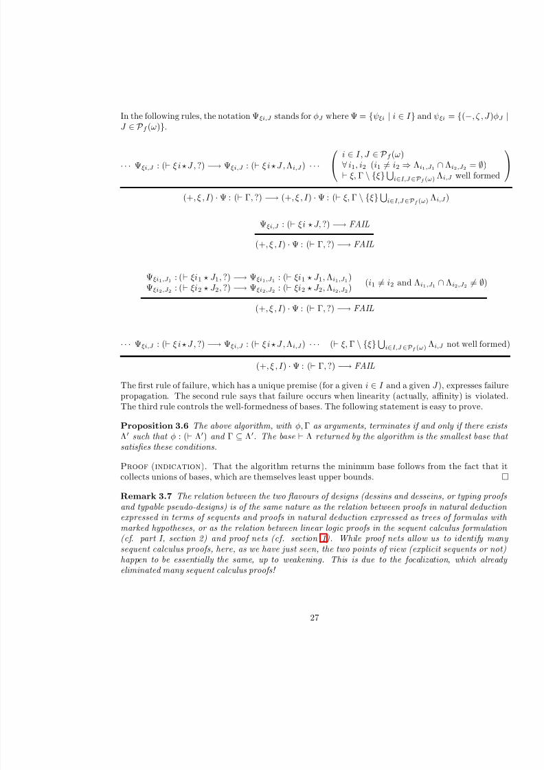
8/3/2019 Pierre-Louis Curien- Introduction to linear logic and ludics, Part II
http://slidepdf.com/reader/full/pierre-louis-curien-introduction-to-linear-logic-and-ludics-part-ii 27/49
In the following rules, the notation Ψξi,J stands for φJ where Ψ = ψξi | i ∈ I and ψξi = (−, ζ , J )φJ |J ∈ P f (ω).
· · · Ψξi,J : (⊢ ξ i ⋆ J , ?) −→ Ψξi,J : (⊢ ξ i ⋆ J , Λi,J ) · · ·
i ∈ I, J ∈ P f (ω)
∀ i1, i2 (i1 = i2 ⇒ Λi1,J 1 ∩ Λi2,J 2 = ∅)⊢ ξ, Γ \ ξ
i∈I,J ∈Pf (ω) Λi,J well formed
(+, ξ , I ) · Ψ : (⊢ Γ, ?) −→ (+, ξ , I ) · Ψ : (⊢ ξ, Γ \ ξ
i∈I,J ∈Pf (ω) Λi,J )
Ψξi,J : (⊢ ξi ⋆ J, ?) −→ FAIL
(+, ξ , I ) · Ψ : (⊢ Γ, ?) −→ FAIL
Ψξi1,J 1 : (⊢ ξi1 ⋆ J 1, ?) −→ Ψξi1,J 1 : (⊢ ξi1 ⋆ J 1, Λi1,J 1)Ψξi2,J 2 : (⊢ ξi2 ⋆ J 2, ?) −→ Ψξi2,J 2 : (⊢ ξi2 ⋆ J 2, Λi2,J 2)
(i1 = i2 and Λi1,J 1 ∩ Λi2,J 2 = ∅)
(+, ξ , I ) · Ψ : (⊢ Γ, ?) −→ FAIL
· · · Ψξi,J : (⊢ ξ i ⋆ J , ?) −→ Ψξi,J : (⊢ ξ i ⋆ J , Λi,J ) · · · (⊢ ξ, Γ \ ξ
i∈I,J ∈Pf (ω) Λi,J not well formed)
(+, ξ , I ) · Ψ : (⊢ Γ, ?) −→ FAIL
The first rule of failure, which has a unique premise (for a given i ∈ I and a given J ), expresses failurepropagation. The second rule says that failure occurs when linearity (actually, affinity) is violated.
The third rule controls the well-formedness of bases. The following statement is easy to prove.
Proposition 3.6 The above algorithm, with φ, Γ as arguments, terminates if and only if there existsΛ′ such that φ : (⊢ Λ′) and Γ ⊆ Λ′. The base ⊢ Λ returned by the algorithm is the smallest base thatsatisfies these conditions.
Proof (indication). That the algorithm returns the minimum base follows from the fact that itcollects unions of bases, which are themselves least upper bounds.
Remark 3.7 The relation between the two flavours of designs (dessins and desseins, or typing proofsand typable pseudo-designs) is of the same nature as the relation between proofs in natural deductionexpressed in terms of sequents and proofs in natural deduction expressed as trees of formulas with marked hypotheses, or as the relation between linear logic proofs in the sequent calculus formulation
(cf. part I, section 2) and proof nets (cf. section 1). While proof nets allow us to identify manysequent calculus proofs, here, as we have just seen, the two points of view (explicit sequents or not)happen to be essentially the same, up to weakening. This is due to the focalization, which alreadyeliminated many sequent calculus proofs!
27

8/3/2019 Pierre-Louis Curien- Introduction to linear logic and ludics, Part II
http://slidepdf.com/reader/full/pierre-louis-curien-introduction-to-linear-logic-and-ludics-part-ii 28/49
Remark 3.8 We can define an injection • mapping pseudo-designs to sets of chronicles ending witha positive action as follows:
Ω• = ∅ ((+, ξ , I ) · ψξi | i ∈ I )• = ǫ
i∈I (+, ξ , I )r | r ∈ ψ•ξi
• = (−, ζ , J )φJ | J ∈ P f (ω)• =
J ∈Pf (ω)(−, ζ , J )r | r ∈ φ•J
Note that the Ω’s disappear during this transformation. In [36] , the designs-desseins are defined assets of chronicles, and properties characterizing the image of the set of designs by the function • aregiven. These properties include:
• coherence : the maximal prefix of any two chronicles of the design which are not prefix of eachother ends with a positive action;
• focalization: a negative action which is not at the root must be of the form (−, ξ i , J ) and its fathermust be of the form (+, ξ , I ), with i ∈ I ;
• subaddress: a positive action (+, ξ , I ) is either such that ξ is an address on the positive side of the
base, or there exist ξ′, i, and J such that ξ = ξ′i, i ∈ J , and (−, ξ′, J ) occurs on the chronicle between (+, ξ , I ) and the root.
Designs have an implicit pointer structure: for each action whose focus is some ξi, one looks forthe action of focus ξ below it in the forest or tree representation of the design, if any, and we saythat the former points to the latter, or is bound to the latter. Otherwise, we say that the action offocus ξi occurs free in the design. It is easily seen that for well-typed designs the two actions musthave opposite signs, and that a free action is necessarily positive and that its focus belongs to theright hand side of the base of the design (cf. Remark 3.2). Moreover, negative actions are alwaysbound and always point to the immediately preceding positive action. These are typical features ofHyland and Ong (HO) games [43] (see [25] for precise comparisons). In [16, 17], a general formalismof such (untyped) HO style strategies over a given alphabet of moves, called abstract B¨ ohm trees, hasbeen developped. Opponent’s moves are letters of the alphabet, while Player’s moves are pairs noted
[a,κ
← ], where a is a letter of the alphabet and where κ is either the symbol that indicates that themove is free, or a natural number that counts the number of Opponent’s moves encountered beforereaching the binder. The designs are abstract Bohm trees constructed on the alphabet consisting ofall the pairs (i, I ) of a natural number and a finite set of natural numbers. The general shape is asfollows (rotating the tree clockwise by 90 degrees):
...( j1, J ′1)Ω...
( j1, J 1)[( j2, I 1), κ2← ]
...(i1, J ′2)Ω
...
(i1, J 2)[( j3, I 2),κ3
← ]
......
...
28
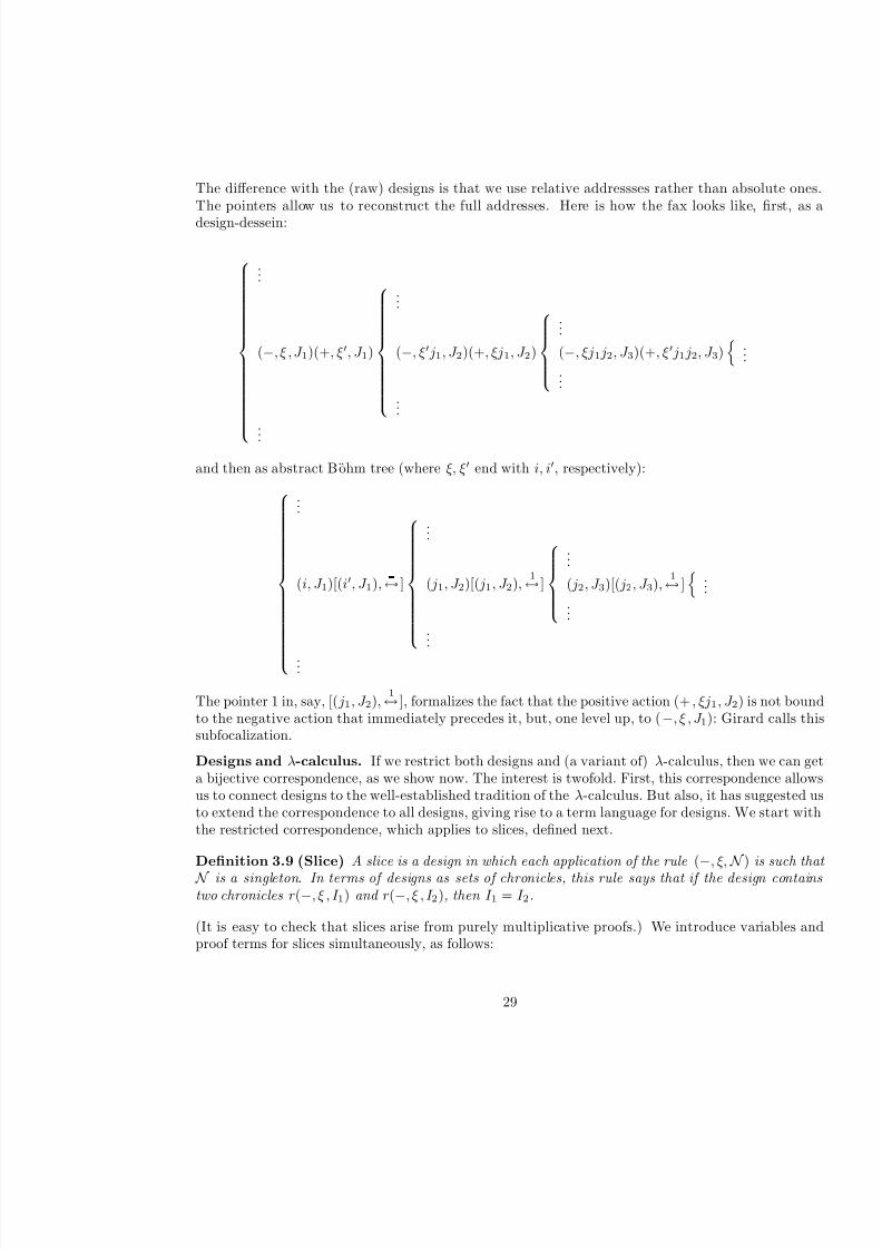
8/3/2019 Pierre-Louis Curien- Introduction to linear logic and ludics, Part II
http://slidepdf.com/reader/full/pierre-louis-curien-introduction-to-linear-logic-and-ludics-part-ii 29/49
The difference with the (raw) designs is that we use relative addressses rather than absolute ones.The pointers allow us to reconstruct the full addresses. Here is how the fax looks like, first, as a
design-dessein:
...
(−, ξ , J 1)(+, ξ′, J 1)
...
(−, ξ′ j1, J 2)(+, ξj1, J 2)
...
(−, ξj1 j2, J 3)(+, ξ′ j1 j2, J 3)
......
....
..
and then as abstract Bohm tree (where ξ, ξ′ end with i, i′, respectively):
...
(i, J 1)[(i′, J 1), ← ]
...
( j1, J 2)[( j1, J 2),1
← ]
...
( j2, J 3)[( j2, J 3),1
← ]
......
...
...
The pointer 1 in, say, [( j1, J 2),1
← ], formalizes the fact that the positive action (+, ξj1, J 2) is not boundto the negative action that immediately precedes it, but, one level up, to (−, ξ , J 1): Girard calls thissubfocalization.
Designs and λ-calculus. If we restrict both designs and (a variant of) λ-calculus, then we can geta bijective correspondence, as we show now. The interest is twofold. First, this correspondence allowsus to connect designs to the well-established tradition of the λ-calculus. But also, it has suggested usto extend the correspondence to all designs, giving rise to a term language for designs. We start withthe restricted correspondence, which applies to slices, defined next.
Definition 3.9 (Slice) A slice is a design in which each application of the rule (−, ξ, N ) is such that
N is a singleton. In terms of designs as sets of chronicles, this rule says that if the design containstwo chronicles r(−, ξ , I 1) and r(−, ξ , I 2), then I 1 = I 2.
(It is easy to check that slices arise from purely multiplicative proofs.) We introduce variables andproof terms for slices simultaneously, as follows:
29

8/3/2019 Pierre-Louis Curien- Introduction to linear logic and ludics, Part II
http://slidepdf.com/reader/full/pierre-louis-curien-introduction-to-linear-logic-and-ludics-part-ii 30/49
Ω : (⊢ Λ) : (⊢ Λ)
P : (⊢ xj : ζj | j ∈ J , Λ′) (Λ′ ⊆ Λ)
λxj | j ∈ J .P : (ζ ⊢ Λ)
· · · M i : (ξi ⊢ Λi) · · ·
i ∈ I ∀ i Λi ⊆ Λ∀ i1, i2 (i1 = i2 ⇒ Λi1 ∩ Λi2 = ∅)x fresh
xM i | i ∈ I : (⊢ x : ξ, Λ)
In the first (resp. second) rule, the cardinal of J (resp. I ) gives the number of head λ’s (resp. thenumber of arguments of the variable). The bases ξ ⊢ Λ and ⊢ Λ are now such that Λ consists of aset of variable declarations of the form x : ζ . Let us place the λ-calculus style syntax that we justintroduced (on the left below) in perspective with the syntax of normal forms of the λ-calculus (onthe right below):
M ::= λxj | j ∈ J .P M ::= λx1 . . . xm.P P ::= xM i | i ∈ I || Ω || P ::= xM 1 . . . M n
The difference lies in the fact that we have freed ourselves from the sequential order of application of the ordinary λ-calculus, and that we now have explicit addresses for the arguments of the application:i is the (relative) address of M i.
Remark 3.10 Combining the bijection from slices to terms just given with the representation of
designs as HO style trees with pointers given above, what we have obtained is a correspondence ofthe same nature as the bijection between λ-terms and λ-terms in De Bruijn notation (see e.g. [1 ]).More precisely, it is exactly a bijection of this kind, replacing De Bruijn indices by other indices thatwe have called B¨ ohm indices in [17 ] (and that have appeared in previous works of Danos-Regnier and
Huet), which are pairs of indices of the form [i,j
← ] where j counts the number of λ’s separating thevariable from its binder and where i serves to identify which among the variables collectively bound by
the binder it is. For example, the B¨ ohm indices of x1 and x2 in λx1, x2.x1λy1.x2 are [1,0
← ]
and [2,1
← ], respectively.
Remark 3.11 It is easily checked that the typable terms are exactly the affine terms, i.e., those in which any variable occurs at most once.
We next move on and give terms for arbitrary designs.
Ω : (⊢ Λ) : (⊢ Λ)
30

8/3/2019 Pierre-Louis Curien- Introduction to linear logic and ludics, Part II
http://slidepdf.com/reader/full/pierre-louis-curien-introduction-to-linear-logic-and-ludics-part-ii 31/49
· · · M i : (ξi ⊢ Λi) · · ·
i ∈ I
∀ i Λi ⊆ Λ∀ i1, i2 (i1 = i2 ⇒ Λi1 ∩ Λi2 = ∅)x fresh
(x.I ) · M i | i ∈ I : (⊢ x : ξ, Λ)
· · · P J : (⊢ xj : ζj | j ∈ J , ΛJ ) · · ·
J ∈ P f (ω)∀ J ΛJ ⊆ Λ
J = λxj | j ∈ J .P J | J ∈ P f (ω) : (ζ ⊢ Λ)
Forgetting now about typing rules, we have the following (untyped) syntax:
M ::= J = λxj | j ∈ J .P J | J ∈ P f (ω)P ::= (x · I )M i | i ∈ I || Ω ||
Since we now have two syntaxes for (pseudo-)designs, we shall refer to the two syntaxes as the abstractsyntax and the concrete syntax, respectively (in the order in which they have appeared in the paper).As an illustration, here is the fax (recursively) expressed in concrete syntax:
Fax ξ,x:ξ′ = I = λyi | i ∈ I .(x · I )Fax ξ′i,yi:ξi | i ∈ I | I ∈ P f (ω) .
In this form, the fax appears as the variable x, in all its possible (hereditarily) η-expansions. Notethe remarkable use of the additive flavour of designs: the fax is ready for any ramification I , i.e. forany possible η-expansion (see Exercise 4.10).
Ordering designs. Two rather natural partial orders can be defined on designs:
• The usual partial information ordering on trees: to increase information, one replaces an Ω with atree = Ω (in the first representation of designs, this amounts to extend a set N in a negative rule).This is reminiscent of the ordering between stable functions defined by the inclusion of their traces(see e.g. [4, chapter 12]).
• The second ordering ⊑ is obtained by adding a second rule for increasing: replace a subtree by a. We shall see that this ordering characterizes the observational order between designs, so we shallcall it the observational ordering. It is reminiscent of the pointwise ordering between Scott continuousfunctions. This ordering is defined formally as follows:
Ω ⊑ φ φ ⊑
· · · ψξi ⊑ ψ′ξi · · · (i ∈ I )
(+, ξ , I ) · ψξi | i ∈ I ⊑ (+, ξ , I ) · ψ′ξi | i ∈ I
· · · φJ ⊑ φ′J · · · J ∈ P f (ω)
. . . , (−, ζ , J )φJ , . . . ⊑ . . . , (−, ζ , J )φ′J , . . .
31

8/3/2019 Pierre-Louis Curien- Introduction to linear logic and ludics, Part II
http://slidepdf.com/reader/full/pierre-louis-curien-introduction-to-linear-logic-and-ludics-part-ii 32/49
φ ⊑ φ
φ1 ⊑ φ2 φ2 ⊑ φ3
φ1 ⊑ φ3
We write φ1 ≤R φ2 (resp. φ1 ≤L φ2) if φ1 ⊑ φ2 has been proved without using the axiom φ ⊑
(resp. Ω ⊑ φ). Thus, φ1 ≤R φ2 is the stable ordering, which we also denote as φ1 ⊆ φ2 (see Exercise3.15).
Remark 3.12 We have the following decomposition property: if φ1 ⊑ φ2, then there exists a φ suchthat φ1 ≤L φ ≤R φ2, obtained by first cutting some subtrees and replacing them by a , and thenby adding some subtrees at some Ω’s. Note that this is a quite natural way of proceeding, since onemight do useless work otherwise, by adding subtrees using axiom Ω ⊑ φ that could then be removedwhile using axiom φ ⊑ Ω. The decomposition is not unique, as we have both Ω ≤L Ω ≤R andΩ ≤L ≤R (see Exercise 3.17 ). Remarkably enough, similar decompositions have been discoveredand exploited elsewhere:
• by Winskel in his analysis of Berry’s stable ordering and bi-domains (see [18 ]), and
• by Laird in his extensional account of the model of sequential algorithms [45, 19 ].
Exercise 3.13 Complete the characterization of designs as sets of chronicles (cf. Remark 3.8 ). (Hint:The only missing conditions are the ones ensuring that the designs are affine.)
Exercise 3.14 Is there a sense in which the concrete syntax and the abstract syntax of pseudo-designsor of designs are in bijective correspondence? (Hints: Pseudo-designs in abstract syntax are morepermissive, e.g., they do not exclude the possibility of a move (+, ξ i , J ) “pointing” to a move (+, ξ , I ).On the other hand, “raw” terms in the concrete syntax are actually all “typable”, in a system wherethe affinity constraint is relaxed.)
Exercise 3.15 Show that, on designs as sets of chronicles (cf. Remark 3.8 ), the stable ordering is setinclusion, and that the extensional ordering can be characterized by the following property: φ1 ⊑ φ2
if and only if whenever r1 = r (−, ξ , I )r′1 ∈ φ1 and r2 = r (−, ξ , I )r′2 ∈ φ2 diverge after some action(−, ξ , I ), then either r′1 = Ω or r′2 = .
Exercise 3.16 We define formally (infinite-depth) designs as ideals (i.e., downwards closed directed subsets of designs) with respect to ⊆. Show that the equation defining the fax admits a least fixed point which is such an ideal.
Exercise 3.17 Let ≤ be the intersection of the partial orders ≤L and ≤R. Show the following moreprecise formulation of the decomposition property: if φ1 ⊑ φ2, then there exist φmin and φmax suchthat:
∀ φ ((φ1 ≤L φ ≤R φ2) ⇔ φmin ≤ φ ≤ φmax ) .
4 Normalization of designs
Normalization is a general machinery that applies to all abstract Bohm trees, hence to designs inparticular. It can be described in various equivalent ways, see [16]. In the affine case, the execution
32

8/3/2019 Pierre-Louis Curien- Introduction to linear logic and ludics, Part II
http://slidepdf.com/reader/full/pierre-louis-curien-introduction-to-linear-logic-and-ludics-part-ii 33/49
is simpler (no copying involved), so we shall describe here (in three disguises) an abstract machinefor designs taking the affine nature of designs into account. The first two presentations of the nor-
malization engine are based on the abstract and concrete syntax for designs, respectively, and use theframework of environment machines, whose states have two components: the code to be run, and theenvironment or context or counter-design. The third version is more visual, and features a simpletoken game. Its main advantage is that it makes the very useful notion of the part of a design visitedduring normalization explicit.
We embark on the first description, for which we shall need the following terminology.
Notation 4.1 We denote by Ψ a finite set ψζ1 , . . . , ψζn of negative pseudo-designs, with the ζ i’spairwise disjoint. We say that Ψ accepts (resp. does not accept) an address ζ if ζ ∈ ζ 1, . . . , ζ n (resp.ζ ∈ ζ 1, . . . , ζ n). If Ψ accepts ζ , i.e., ζ = ζ j for some j, we use the notation Ψζ for ψζj . We alsonote simply ψ for ψ. Finally, if Ψ accepts ζ , we note Ψ \ ζ = Ψ \ ψζ .
We start with a design φ : (⊢ ξ, Λ1) to be normalized against a design ψ : (ξ ⊢ Λ2) (with Λ1 andΛ2 pairwise disjoint), which we call its counter-design . The normalization should produce a designbased on ⊢ Λ1, Λ2 (think of a cut rule).
The machine has states of the form φ | Ψ, and execution consists in applying the following statetransformation, which we call the weak reduction rule (by contrast to strong reduction, introducedbelow):
(R) (+, ξ , I ) · Ψ′ | Ψ −→ Ψξ,I | Ψ′ ∪ (Ψ \ ξ) (Ψ accepts ξ)
Notice that we throw away all of Ψ ξ except for Ψξ,I . In particular, the negative actions (−, ξ , J ) of Ψare not needed. That we can do this safely will be justified by Proposition 4.18.
The initial state is φ | ψ. It is important to keep Ψ \ ξ in order to handle subfocalizations, asillustrated by the example below (where ζ = ξi1i, for some i ∈ I 1):
φ =
· · ·
· · ·
(+, ζ , J )
(−, ξi1, I 1) · · ·
· · ·
(−, ξi2, I 2) · · ·
(+, ξ , I ) ψ = · · ·
· · ·
· · ·
(+, ξi2, I 2)
(−, ζ , J ) · · ·
(+, ξi1, I 1)
(−, ξ , I ) · · ·
or:
φ = (+, ξ , I ) · Ψ′
with Ψ′ = . . . , (−, ξi1, I 1)φ2, . . . , (−, ξi2, I 2) · · · , . . .with φ2 = (+, ζ , J ) · Ψ2
ψ = . . . , (−, ξ , I )φ1, . . .with φ1 = (+, ξi1, I 1) · Ψ1
with Ψ1 = . . . , (−, ζ , J )φ3, . . .with φ3 = (+, ξi2, I 2) · · ·
Execution goes as follows:
33

8/3/2019 Pierre-Louis Curien- Introduction to linear logic and ludics, Part II
http://slidepdf.com/reader/full/pierre-louis-curien-introduction-to-linear-logic-and-ludics-part-ii 34/49
φ | ψ −→ φ1 | Ψ′ ∪ (ψ \ ξ) = φ1 | Ψ′
−→ φ2 | Ψ1 ∪ (Ψ′ \ ξi1)−→ φ3 | Ψ2 ∪ (Ψ1 \ ξ) ∪ (Ψ′ \ ξi1)
At state φ3 | Ψ2 ∪ (Ψ1 \ ξ) ∪ (Ψ′ \ ξi1), it is essential to have Ψ ′ available, as the head action of φ3
corresponds to a head action of Ψ′ and not of Ψ2, i.e., when normalization reaches (+, ξi2, I 2), thecorresponding negative action on the left is not found above (+, ζ , J ), but above (+, ξ , I ).
The machine stops when it reaches an Ω (which one should interpret as waiting for more informationfrom the context), a (that indicates convergence), or a state (+, ξn, I n) · Ψ′
n | Ψn such that Ψn
does not accept ξn (in λ-calculus terminology, this means reaching a head variable). In all three cases,we have found the root of the normal form of φ | ψ (see also Remark 4.4).
We can go on, and perform “strong reduction”, by relaunching the machine in order to get pro-gressively, on demand, the chronicles of the normal form, and not only the first positive action of thenormal form. This can be formalized by indexing the state by the chronicle q of the normal formunder exploration. The index remains invariant in the rule (R), which is thus reformulated as:
(R) (+, ξ , I ) · Ψ′ | Ψq −→ Ψξ,I | Ψ′ ∪ (Ψ \ ξ)q (Ψ accepts ξ)
Initially, the index is the empty chronicle ǫ. The chronicle is extended using the following rule (S stands for strong reduction):
(S) (+, ξ , I ) · Ψ′ | Ψq −→ Ψ′ξi,J | Ψq(+,ξ,I )(−,ξi,J ) (Ψ does not accept ξ and i ∈ I )
Note that this rule is non-deterministic: the choice of i, J is left to the Opponent of the normal form,he has to say which branch of the normal form he intends to explore.
The two other termination cases remain termination cases in this setting, and are formalized asfollows:
Ω | Ψq −→ ! q Ω | Ψq −→ ! q
Read ! q Ω (resp. ! q) as an output, saying that the chronicle q Ω (resp. q) belongs to the normalform. As for rule (S), we can read that q(+, ξ , I ) belongs to the normal form, but in addition we knowthat the normal form contains a chronicle of the form q(+, ξ , I )(−, ξ i , J )κi,J for all i ∈ I and J , andmay start an exploration in order to find any of these actions κi,J .
We denote the normal form of φ | ψ by [[φ, ψ]], or simply [[φ, ψ]], and more generally, wedenote the normal form of φ | Ψ (see Definition 4.2) by [[φ, Ψ]]. As a set of chronicles, it is obtainedby collecting all the results of execution:
[[φ, Ψ]] = q(+, ξ , I ) | ∃ Ψ′, Ψ′′ φ | Ψǫ −→⋆ (+, ξ , I ) · Ψ′ | Ψ′′q
∪ q Ω | φ | Ψǫ −→⋆ ! q Ω∪ q | φ | Ψǫ −→⋆ ! q∪ q Ω | computation does not terminate and q is the maximal index reached
Note that we have added a second case of divergence: the divergence due to the cases where themachine does not terminate. To be more precise, we are speaking of non-termination due to rule
34

8/3/2019 Pierre-Louis Curien- Introduction to linear logic and ludics, Part II
http://slidepdf.com/reader/full/pierre-louis-curien-introduction-to-linear-logic-and-ludics-part-ii 35/49
(R) only (at index q), not of non-termination due to a potentially infinite branch of the normal form(recall that we are in a demand-driven setting).
Therefore, there are two sorts of Ω in the normal form: those that are “created” (by the magicof a mathematical formula, not by some computation observed in a finite time), and those that comefrom the Ω′s explicitly present in φ or Ψ. The overloading of the two situations is really what makesthe difference between Ω and that otherwise behave in a dual way (cf. e.g. the definition of ≤L
and ≤R). It is also the reason for the name Fid given by Girard to the partial design Ω: you musthave faith (Fides in Latin) to wait for a result that might never come.
We still have to establish that [[φ, Ψ]] is a design, not only a pseudo-design, and hence we shouldexhibit a typing proof of [[φ, Ψ]]. We first have to type the states of the machine, which we can alsocall nets, using Girard’s terminology inspired from proof nets. We have seen that a state, or net,consists of a positive design φ and a collection Ψ′ of negative designs. We stick to this situation inthe following definition.
Definition 4.2 A (positive) net is given by a positive design φ : (⊢ Λ), called the principal design ofthe net, and a finite set Ψ of negative designs such that:
1. the addresses appearing in the bases of φ and of the elements of Ψ are pairwise disjoint or equal;
2. an address may appear at most twice in these bases;
3. if an address appears twice, then it appears once on the left of ⊢ and once on the right of ⊢,thus forming a cut;
4. The graph whose set of vertices is φ ∪ Ψ (or the associated set of bases) and whose edges arethe cuts is acyclic.
We denote the net by φ | Ψ.
Girard requires moreover connectivity. We do not make this requirement explicit here, but it isclear that what interests us is the connected component of φ. In this connected component, all theξ’s on the left of ⊢ are cut. This is easily shown by induction on the length of a path starting at ⊢ Λ.The only interesting case is when the path has reached a node of the form ξ′ ⊢ Λ′ and proceeds fromthere to a node of the form ξ′′ ⊢ Λ′′ with a cut on ξ′. But then by induction and by condition 2, thelatter node must have been visited by the path earlier and must be the one that witnesses that ξ′ iscut. Therefore, we know by induction that ξ′′ is cut.
Hence all the non-cut addresses of the designs of the connected component stand to the right of⊢, in φ or in one of the elements of Ψ. Let Λ be the set of these addresses. We set φ | Ψ : (⊢ Λ). (Itis thus the connected component that we actually type, but it is more convenient not to throw awayexplicitly the elements of the other connected components.)
Proposition 4.3 If φ | Ψ is a net and if φ | Ψ : (⊢ Λ), then [[φ, Ψ]] : (⊢ Λ).
Proof. We only prove that rule (R) preserves typing, which is enough to prove the statement in thecase of a net of type ⊢ (see Remark 4.4). Suppose that (+, ξ , I ) · Ψ′ | Ψ : (⊢ Λ). We have to proveΨξ,I | Ψ′ ∪ (Ψ \ ξ) : (⊢ Λ).
Condition 4. We have (+, ξ , I )·Ψ′ : (⊢ ξ , . . .), and Ψ : (. . . , (ξ ⊢ . . .), . . .), hence Ψ′ : (ξi ⊢ . . .) | i ∈ I and (Ψ)ξ,I : (⊢ ξ ⋆ I , . . .). Thus we remove the bases (⊢ ξ , . . .) and (ξ ⊢ . . .) from the graph and replace
35

8/3/2019 Pierre-Louis Curien- Introduction to linear logic and ludics, Part II
http://slidepdf.com/reader/full/pierre-louis-curien-introduction-to-linear-logic-and-ludics-part-ii 36/49
them by the base (⊢ ξ ⋆ I , . . .) and the bases (ξi ⊢ . . .). The edge that connected (⊢ ξ , . . .) to (ξ ⊢ . . .)is replaced by edges that connect (⊢ ξ ⋆ I , . . .) to each of the (ξi ⊢ . . .)’s. Note that these new edges
form a connnected configuration. The edges that once arrived to ( ξ ⊢ . . .) now arrive to (⊢ ξ ⋆ I , . . .),and those that arrived to (⊢ ξ , . . .) are now either disconnected or arrive to one of the ( ξi ⊢ . . .)’s. Ifthere was a cycle in the new graph, one would then easily construct one in the former graph (to whichwe can go back by amalgamating the bases (ξi ⊢ . . .)).
Conditions 2 and 3. The two occurrences of ξ disappear, and are replaced by pairs of occurrences of each ξi.
Remark 4.4 A consequence of the previous proposition is that when the weak reduction machinestarting from φ | Ψ : (⊢ Λ) stops in a state (+, ξn, I n) · Ψ′
n | Ψn, where Ψn does not accept ξn, thenξn ∈ Λ. Indeed, by type preservation we have (+, ξn, I n) · Ψ′
n | Ψn : (⊢ Λ). On the other hand we have(+, ξn, I n) · Ψn : (⊢ Λ0) and Ψ′
n : ζ 1 ⊢ Λ1, . . . , ζ m ⊢ Λm with ξn ∈ Λ0 and ξn ∈ ζ 1, . . . , ζ m, that is,ξn is not cut. Hence ξn ∈ Λ. In particular, when Λ is empty, then the weak reduction machine can
only end with an Ω or a , and there is no need for strong reduction – this situation is quite similar to the situation in a functional programming language like CAML, whose implementation is based on weak reduction, which is complete for evaluating observable results of basic types. In the sequel, weshall often place ourselves in such a situation, with φ : (⊢ ξ), Ψ = ψ, and ψ : (ξ ⊢), for some ξ.
Definition 4.5 For φ : (⊢ ξ) and ψ : (ξ ⊢), we write φ⊥ψ (or ψ⊥φ) if [[φ, ψ]] = and we saythat φ is orthogonal to ψ. For a set A of designs on the same base ⊢ ξ (resp. ξ ⊢), we writeA⊥ = ψ | ∀ φ ∈ A φ⊥ψ (resp. A⊥ = φ | ∀ ψ ∈ A φ⊥ψ), and we write simply φ⊥ for φ⊥.
The definition of orthogonality is not limited to bases of the form ⊢ ξ and ξ ⊢: more generally,if φ : (⊢ ξ1, . . . , ξn), ψ1 : (ξ1 ⊢) ,. . . , ψn : (ξn ⊢), and [[φ, ψ1, . . . , ψn]] = , then we say that φ isorthogonal to ψ1, . . . , ψn.
Exercise 4.6 Show that is the only design which is orthogonal to the skunk (cf. Definition 3.4).
Exercise 4.7 Show that if I ⊆ J , φ : (⊢ I ) and ψj : ( j ⊢) for all j ∈ J , then [[φ, ψi | i ∈ I ]] =[[φ, ψj | j ∈ J ]] (taking φ to be of type ⊢ J on the right side of this equality).
Exercise 4.8 Rule (R) does not make explicit the alternation between (the subdesigns of) φ and ψ:the positive actions that guide computation are indeed alternating. The following variant of rule (R)(to be applied systematically after the second step) makes this alternation explicit:
(R’)(+, ξ , I ) · Ψ′ | Ψ −→ (+, ξ1, I 1) · Ψ′
1 | Ψ1 (Ψ1 accepts ξ1)
(+, ξ1, I 1) · Ψ′1 | Ψ1 −→ (Ψ1)ξ1,I 1 | Ψ′
1 ∪ (Ψ \ ξ)
(1)Using this rule, check that the execution of the above example unrolls now as follows:
φ | ψ −→ φ1 | Ψ′−→ φ2 | Ψ1−→ φ3 | (Ψ′ \ ξi1) ∪ Ψ2
(2) Show formally that the machine obtained with (R’) is equivalent to the one defined with (R).
36

8/3/2019 Pierre-Louis Curien- Introduction to linear logic and ludics, Part II
http://slidepdf.com/reader/full/pierre-louis-curien-introduction-to-linear-logic-and-ludics-part-ii 37/49
Exercise 4.9 What about normalizing a negative design against a negative design? (Hint: Use strong reduction.)
Normalization in concrete syntax. How does normalization look like, when described in termsof the concrete rather than the abstract syntax? We let the reader convince himself that the affine(weak reduction) machine given above gets mapped through the bijective correspondence between theconcrete syntax and the abstract syntax to the following one:
(x · I )M i | i ∈ I | ρ ∪ (x ← . . . , I = λxi | i ∈ I .P I , . . . −→ P I | ρ ∪ (i∈I
(xi ← M i)
In this rule, ρ stands for an environment which is a function from a finite set of variables to terms,described as a set of bindings of the form ( x ← M ), and the union symbols stand for disjoint unions.
The initial state corresponding to φ | ψ is here of the form P | (x ← M ), for some P : (⊢ x : ξ, Λ1)and M : (ξ ⊢ Λ2).
The crucial use of the affine restriction lies in the fact that x does not occur in any of the M i’s,and hence that the binding for x is consumed after the application of the rule. But the general caseof non necessarily affine pseudo-designs in concrete syntax is not much more difficult to describe, bymeans of a very similar abstract machine, which is an instance of the (stack-free) Krivine machinedescribed in [16]:
(x · I )M i | i ∈ I | ρ −→ P I | ρI ∪ (i∈I
(xi ← M i | ρ)
where ρ(x) = . . . , I = λxi | i ∈ I .P I | ρI , . . ..
The main change with respect to the affine machine is that now an environment maps variables to
closures, which are used in the implementation of functional programming languages to keep track of a code together with the environment for its free variables. Note that we keep now all the environmentto be available for the M i’s, even the binding for x, as x may appear in any of the M i’s.
Exercise 4.10 Show that, for any positive P of appropriate type, the (strong version of) the machinereduces P | x′ ← Fax ξ,x:ξ′ to P [x′ ← x] ( α-renaming).
Token machine: normalization as a visit. We now give our third version of normalization, whichis more intuitive. It is described in terms of pushing a token through the designs (see also [24]). Underthis interpretation, the net formed of φ and ψ remains fixed, and information (in the form of a markor token placed on a single node) flows through it. Initially, the token is placed at the root of φ. Inorder to identify the nodes of φ and ψ, we introduce the following notation for occurrrences of actions:
(Ω)ǫ = Ω ()ǫ =
((+, ξ , I ) · ψξi | i ∈ I )ǫ = (+, ξ , I ) ((+, ξ , I ) · ψξi | i ∈ I )iu = (ψξi)u
((−, ζ , J )φJ | J ∈ P f (ω))J = (−, ζ , J ) ((−, ζ , J )φJ | J ∈ P f (ω))J 1u = (φJ )u
37

8/3/2019 Pierre-Louis Curien- Introduction to linear logic and ludics, Part II
http://slidepdf.com/reader/full/pierre-louis-curien-introduction-to-linear-logic-and-ludics-part-ii 38/49
Thus an occurrence is a word over an alphabet whose letters are either i, I , or 1, and which appearin the order i1I 11i2I 21i3 . . .. The token is formalized as an occurrence u of either φ or ψ, which we
write (L, u) (resp. (R, u)) if the occurrence is in φ (resp. ψ). The token machine maintains a set of pairs ((L, u), (R, v)) where the actions (φ)u and (ψ)v are opposite, and where each u, v occurs at mostonce. These pairs are called bindings (in a sequent calculus description of cut-elimination (cf. part I,section 3), they represent the successive cuts). Initially, the token is at occurrence (L, ǫ), and the setof bindings is empty. The token game follows the tree structure and the pointer structure of φ and ψ,and the bindings. The rules are as follows:
• from (L, ǫ), with (φ)ǫ = (+, ξ , I ), move to (R, I ) and place (((L, ǫ), (R, I )) in the list of bindings;
• from (R, u) such that (ψ)u is a negative action, move to (R, u1);
• from (R, u) such that (ψ)u = (+, ζ i , I ), u points to v, and ((L, v′), (R, v)) is in the set of bindings,then move to (L, v′ i I ) and add ((L, v′ i I ), (R, u)) to the set of bindings;
• from (L, u) such that (φ)u = (+, ζ i , I ), u points to v, and ((L, v), (R, v′)) is in the set of bindings,then move to (R, v′ i I ) and add ((L, u), (R, v′ i I )) to the set of bindings;
• from (L, u) such that (φ)u is a negative action, move to (L, u1).
For example, the execution of our running example goes as follows, with the corresponding actions(recall that ζ = ξi1i):
(L, ǫ) (R, I ) (R, I 1) (L, i1I 1) (L, i1I 11) (R, I 1iJ ) (R, I 1iJ 1) (L, i2 I 2) . . .
(φ)ǫ (ψ)I ψI 1 (φ)i1I 1 (φ)i1I 11 (ψ)I 1iJ (ψ)I 1iJ 1 (φ)i2I 2 . . .= = = = = = = = . . .
(+, ξ , I ) (−, ξ , I ) (+, ξi1, I 1) (−, ξi1, I 1) (+, ζ , J ) (−, ζ , J ) (+, ξi2, I 2) (−, ξi2, I 2) . . .
The actions visited during normalization are all the actions (φ)u such that the token reachesposition (L, u) and all the actions (ψ)u such that the token reaches position (R, u). They determinetwo designs φ1 ⊆ φ and ψ1 ⊆ ψ (the pull-back , see Theorem 4.13) which form a balanced pair (i.e.,their sets of actions are dual). Remarkably, there is a converse to this (see Proposition 4.19).
Exercise 4.11 Show that the first and third versions are equivalent, i.e., that they yield the sameresult of normalization for every pair of designs φ : (⊢ ξ) and ψ : (ξ ⊢). (Hint: At some point,Proposition 4.18 has to be used.)
Analytical theorems. These are the following theorems:
1. the associativity theorem , that corresponds to Church-Rosser property;2. the separation theorem , that corresponds to (an affine version of) Bohm’s theorem;
3. the monotonicity theorem , that corresponds to the syntactic continuity theorem in the λ-calculus,due to Welch and Levy, which states that Bohm trees commute with contexts (see e.g. [4, section2.3]);
38

8/3/2019 Pierre-Louis Curien- Introduction to linear logic and ludics, Part II
http://slidepdf.com/reader/full/pierre-louis-curien-introduction-to-linear-logic-and-ludics-part-ii 39/49
4. the stability theorem , that corresponds to the syntactic stability theorem of the λ-calculus, dueto Berry, which states that the Bohm tree function from partial terms to partial Bohm trees is
stable (it enjoys actually the stronger property of being sequential, see e.g. [4, section 2.3]).
Remark 4.12 The tradition behind the third and the fourth theorems is more widely known through their outsprings in denotational semantics [ 4] : Scott ’s continuous semantics, Berry ’s stable seman-tics. Berry’s semantics was clearly motivated by the stability theorem, while the syntactic continuitytheorem seems rather to have given an additional a posteriori confirmation of the pertinence of Scott’stheory, which was initially suggested by results in recursion theory (theorems of Rice and of Myhill-Shepherdson).
We start with the stability theorem.
Theorem 4.13 (Stability) If r is a chronicle of [[φ, ψ]], then there exist φ0 ⊆ φ, ψ0 ⊆ ψ minimum,called the pull-back of r along normalization, such that r ∈ [[φ0, ψ0]].
Proof. We mark all the nodes visited during the (deterministic) normalization in order to obtain r:all these nodes must be present, otherwise normalization would diverge, moreover they suffice (justadding Ω’s above non visited negative actions following visited positive actions, in order to obtainpseudo-designs). One also has to check that these pseudo-designs are actually designs (omitted).
It is well-known that stability described in terms of pull-backs as above entails stability in algebraicterms: if φ1, φ2 ⊆ φ and ψ1, ψ2 ⊆ ψ, then
[[φ1 ∩ φ2, ψ1 ∩ ψ2]] = [[φ1, ψ1]] ∩ [[φ2, ψ2]]
(set intersection of the designs as sets of chronicles). In particular, for φ1, φ2 ⊆ φ based on, say, ⊢ ξ,and ψ based on ξ ⊢, we have:
(φ1 ∩ φ2)⊥ψ ⇔ φ1⊥ψ and φ2⊥ψ .
The same properties are true for any bounded intersection of φk’s, ψk’s.
Theorem 4.14 (Separation) The following equivalence holds, for all designs φ1, φ2 on the samebase: φ1 ⊑ φ2 if and only if φ⊥1 ⊆ φ⊥2 .
Proof. Let φ1 ⊑ φ2. By transitivity, we may restrict our attention to ≤R and to ≤L. Let ψ be suchthat φ1⊥ψ. Let φ be the part of φ1 that is effectively visited during normalization (cf. the stabilitytheorem). If φ1 ≤R φ2, φ is also included in φ2, and we thus also have φ2⊥ψ. If φ1 ≤L φ2, and if φ isnot included in φ2, then some subtree of φ has been replaced by , but then the normalization willmeet this , i.e., normalization is more rapid with φ2 than with φ1.
Reciprocally, suppose that φ⊥1 ⊆ φ⊥2 , and that there exists a pair of chronicles, one in φ1, the otherin φ2, that are not prefix of each other. Their intersection q ends with a negative action, since after
a positive action, the set of negative actions depends only on the previous positive action, not on thedesign. By Exercise 3.15, it suffices to check that the only possible configurations are the following:either the branch that continues in φ1 is reduced to Ω, or the branch that continues in φ2 is reducedto . We use the following construction, that allows us to explore a chronicle interactively. We firstdefine the (dual) view of a chronicle (supposing that the design is based on ⊢ ǫ, for simplicity):
39

8/3/2019 Pierre-Louis Curien- Introduction to linear logic and ludics, Part II
http://slidepdf.com/reader/full/pierre-louis-curien-introduction-to-linear-logic-and-ludics-part-ii 40/49
view (r(−, ζ , J )) = view (r)(+, ζ , J )
view ((+, ǫ , I )) = (−, ǫ , I )view (r(−, ξ , J ) · · · (+ξj,I )) = view (r)(+, ξ , J )(−,ξj,I ))
We next define the following designs (as sets of chronicles):
• Oppr (for a positive chronicle r) consists of the set of the views of the prefixes of r, plus view (r);we have that Oppr is the minimum design such that r⊥Oppr, by construction;
• Oppq (for a negative chronicle) consists of the set of the views of the prefixes of q, plus all thechronicles of the form view (q)(−, ζ , J )Ω; we have that Oppq is the minimum design such that(q)⊥Oppq, by construction.
Back to the proof. Let q be the maximum common prefix. We distinguish three cases:
1. q ∈ φ1. Then we have (q)⊥Oppq , hence φ1⊥Oppq. We should then have φ2⊥Oppq, but theinteraction between φ2 and Oppq follows q, and then has not “enough fuel” to continue in φ2.This case is thus impossible.
2. r = q(+, ξ , I ) ∈ φ1. We reason similarly. We have r⊥Oppr, and the interaction has not “enoughfuel” to continue in φ2, except if q ∈ φ2 (second allowed configuration).
3. q Ω ∈ φ1. This is the first allowed configuration.
Remark 4.15 We have made a crucial use of the affinity condition in the proof of the separation theorem. Consider a chronicle of the form q (+, ξ)(−, ξi1) . . . (+, ξ)(−, ξi2). . ., forgetting ramifications
for simplicity. Then we collect two views
view (q) (−, ξ) (+, ξi1) and view (q) (−, ξ) (+, ξi2)
that do not fit together in a design, since a strategy answers an Opponent’s move uniquely.
Theorem 4.16 (Associativity) Let φ, Ψ1, and Ψ2 be such that φ and Ψ1 ∪ Ψ2 form a net. Thenwe have:
[[[[φ, Ψ1]], Ψ2]] = [[φ, Ψ1 ∪ Ψ2]] .
Proof (indication). Let r be a chonicle of [[φ, Ψ1 ∪ Ψ2]], with pullback φ′, Ψ′1, Ψ′
2. One shows thatr can be pulled back along normalization of [[φ, Ψ1]] | Ψ2, with a pullback φ′, Ψ′′
2 such that Ψ′2 = Ψ ′′
2
and the pullback of φ′ along normalization of [[φ, Ψ1]] is φ′, Ψ′1. A similar statement can be proved in
the other direction. These statements are best proved using a strong reduction version of the tokenmachine. Intuitively, the machine execution corresponding to the left hand side does some extra work
with respect to the execution on the right hand side net: as the execution proceeds, it records thepart of the normal form of the net φ | Ψ1 that is being built.
Theorem 4.17 (Monotonicity) If φ1 ⊑ φ2 and ψ1,1 ⊑ ψ2,1, . . . , ψ1,n ⊑ ψ2,n, then
[[φ1, ψ1,1, . . . , ψ1,n]] ⊑ [[φ2, ψ2,1, . . . , ψ2,n]] .
40

8/3/2019 Pierre-Louis Curien- Introduction to linear logic and ludics, Part II
http://slidepdf.com/reader/full/pierre-louis-curien-introduction-to-linear-logic-and-ludics-part-ii 41/49
Proof. We have to show that [[φ1, ψ1,1, . . . , ψ1,n]]⊥Ψ implies [[φ2, ψ2,1, . . . , ψ2,n]]⊥Ψ, for all Ψ. Byassociativity, this amounts to deduce [[φ2, ψ1,1, . . . , ψ1,n∪Ψ]] = from [[φ1, ψ2,1, . . . , ψ2,n∪Ψ]] = ,
which is a consequence of the assumptions (recall that any increase in the order ⊑ only fastensnormalization).
We end the section by showing that normalization explores only multiplicative parts.
Proposition 4.18 The pull-back of a chronicle is always a slice (cf. Definition 3.9 ). More generally,the pullback of a slice is a slice. Moreover, each node of this slice is visited only once.
Proof. We limit ourselves to a normalization between φ : (⊢ ξ) and ψ : (ξ ⊢) (and hence to thepullback of ). For two negative actions (−, ξ i , I 1) and (−, ξ i , I 2) with the same focus and above thesame positive action (+, ξ , I ) to be visited, we need on the other side two positive actions (+,ξi,I 1)and (+, ξ i , I 2) pointing to the same negative action (−, ξ , I ). We reason by minimal counter-example,where minimality is taken with respect to the time at which the hypothetical second visit takes place.
Typing excludes that these two positive actions be one above another (the address is consumed afterthe first visit). Thus they must appear in incompatible positions in the tree, and the divergence startsfrom a positive action. Then typing implies that the first two negative actions on the two divergingpaths must have the same focus (disjointness of contexts). These two actions must have been visitedbefore, a contradiction to minimality. Note that the reasoning applies a fortiori with I 1 = I 2, whichproves the last part of the statement.
Notice that Proposition 4.18 implies that the token machine terminates on finite designs (a propertywhich is obvious with our first formalization of normalization).
Proposition 4.19 If two finite slices φ and ψ are such that their underlying set of actions are oppo-site, then the normalization of φ | ψ visits all of φ and ψ.
Proof. (A more general statement is proved in [35, Proposition 1]). Note that since we deal with
slices, we can omit the ramifications, and name the actions simply with their sign and their focus. Wesay that two slices satisfying the condition in the statement form a balanced pair : (+, ξ) (resp. (−, ξ))occurs in φ if and only if (−, ξ) (resp. (+, ξ)) occurs in ψ.
The proof is by contradiction. If the normalization stops before having explored φ and ψ entirely,it stops having visited φ′ ⊆ φ and ψ′ ⊆ ψ, where φ′ and ψ′ form a balanced pair, and we have, say,φ′ = φ, but then also ψ′ = ψ since φ′ and ψ′ have the same addresses. Consider the actions on theborder, i.e., which are not in φ′ nor in ψ′, but whose father is in φ′ or ψ′: they must be negative,since otherwise the normalization procedure would have visited them. So let us pick an action (−, ξ1)on the border, say in φ \ φ′. Then also (+, ξ1) occurs somewhere in ψ \ ψ′. Consider the chronicle(determined by) (+, ξ1), and let (−, ξ2) be the action of this chronicle which lies on the border. Wecan continue this and build an infinite sequence of actions (−, ξn). Now, for all n, we have ξn = ξ′nin
and (+, ξ′n) ∈ φ′ ∪ ψ′, for some ξ′n and in (focalization condition, cf. Remark 3.8). We also havethat (−, ξ′n) ∈ φ′ ∪ ψ′, since φ′ and ψ′ form a balanced pair. The action (−, ξ′n) appears on the
chronicle (+, ξn) (subaddress condition), and hence by construction (−, ξ′n) occurs before (+, ξ′n+1) onthis chronicle. It follows that (−, ξ′n) is visited before (+, ξ′n+1) during normalization. Since (+, ξ′n) isvisited right before (−, ξ′n), we have that (+, ξ′n+1) is visited strictly after (+, ξ′n). But this contradictsthe termination of the normalization procedure, which as we have seen is a consequence of Proposition4.18.
41

8/3/2019 Pierre-Louis Curien- Introduction to linear logic and ludics, Part II
http://slidepdf.com/reader/full/pierre-louis-curien-introduction-to-linear-logic-and-ludics-part-ii 42/49
Several characterizations of those designs φ which can be entirely visited during normalizationagainst a counter-design ψ are given in [26].
Exercise 4.20 Show that in presence of the separation property, associativity is equivalent to (ageneral formulation of) the following statement (called closure principle). If φ : (⊢ ξ) and ψ : (ξ ⊢ λ),then [[φ, ψ]] is the unique design φ′ such that [[φ′, ψ′]] = [[φ, ψ, ψ′]] for all ψ′ : (λ ⊢).
5 Behaviours
A positive behaviour on a base ⊢ Λ (resp. a negative behaviour on a base ξ ⊢ Λ) is a set G of designsof type (⊢ Λ) (resp. (ξ ⊢ Λ)) closed by taking the bi-orthogonal, i.e., G = G⊥⊥. In most cases, wesuppose that the base is of the form ⊢ ξ or ξ ⊢. Equivalently, a behaviour, say, on the base ⊢ ξ (resp.(ξ ⊢)) is a set of the form A⊥, where A is an arbitrary set of designs of type (ξ ⊢) (resp. (⊢ ξ)).Throughout the section, we take ξ = ǫ. Here are some examples of behaviours:
• If A = ∅, then A⊥ is the set of all the designs of type (ǫ ⊢) (resp. (⊢ ǫ)): this behaviour isdenoted ⊤.
• If A = ⊤ is negative (resp. positive), it is easy to see that A⊥ = Dai (resp. A⊥ = Dai −).Hence a behaviour is never empty, it always contains Dai or Dai −.
• If φ is a design, the smallest behaviour that contains it is:
φ⊥⊥ = φ′ | φ ⊑ φ′ .
Indeed, for any A, we have A⊥ = φ′ | A ⊆ φ′⊥, so in particular φ⊥⊥ = φ′ | φ⊥ ⊆ φ′⊥ =φ′ | φ ⊑ φ′.
Below, we list a few closure properties of behaviours, which are easily checked:
• If G is a behaviour and if φ ∈ G and φ ⊑ φ′, then φ′ ∈ G (by the separation theorem).
• If G is a behaviour and if φk is a bounded family of designs (considered as sets of chronicles) ofG, i.e., ∃ φ (∀ k φk ⊆ φ)), then their intersection is a design of G (by the stability theorem).
• Every intersection of behaviours is a behaviour (as, say, A⊥ ∩ B⊥ = (A ∪ B)⊥).
Definition 5.1 (incarnation) If G is a behaviour and if φ ∈ G, we call the incarnation of φ in Gthe smallest design ⊆ φ of G (whose existence follows from the second closure property listed above).We denote it as |φ|G or simply |φ|. An incarnated design is a design φ such that φ = |φ|. We set|G| = φ ∈ G | φ = |φ|G.
The stability theorem and the definition of behaviour allow us to give a more operational char-acterization of the incarnation: |φ|G is the set of chronicles that are visited during a normalizationof φ against some design ψ of G⊥ (different designs may be used for witnessing the visit of differentchronicles).
Incarnation is clearly contravariant: if G ⊆ H and φ ∈ G, then |φ|H ⊆ |φ|G. The extreme case is|ψ|⊤ = Skunk (negative base).
42

8/3/2019 Pierre-Louis Curien- Introduction to linear logic and ludics, Part II
http://slidepdf.com/reader/full/pierre-louis-curien-introduction-to-linear-logic-and-ludics-part-ii 43/49
Lemma 5.2 For any behaviour, we have G⊥ = |G|⊥.
Proof. We get G⊥ ⊆ |G|⊥ by contravariance. Now let ψ ∈ |G|⊥ and let φ ∈ G. Then ψ⊥|φ|G, andhence ψ⊥φG by monotonicity.
Additives. We now have enough material to return to types and logic. The paradigm is that ofbehaviours as types. The rest of the section is devoted to constructions on behaviours, correspondingto those of linear logic, and more. Some of these constructions are reminiscent of phase semantics (cf.part I, section 5), but the present framework is obviously much richer.
Definition 5.3 (Intersection, Union) If Gk is a family of behaviours on the same base, the set intersection of this familly is a behaviour (cf. above), that we call the intersection of these behaviours,notation
k Gk. We define the union of behaviours
k Gk as the bi-orthogonal of their set union:
k Gk = (
k Gk)⊥⊥.
The ordinary additives correspond to the particular case where the connectives are applied todisjoint behaviours – a notion that we define now (using some of the designs of Definition 3.4).
Definition 5.4 (Directory) A directory is a set of ramifications (i.e., a subset of P f (ω)). If G isa positive behaviour on ⊢ ǫ, we define the directory Dir (G) as follows: Dir (G) = I | Ram (ǫ,I ) ∈ G.
If G is negative, we define Dir (G) by the equation Dir Dir (G) = |Dai −|G.
The following properties show the relevance of this definition:
• If G is positive, then Dir (G) is the set of the I ’s such that G contains a design beginningwith (+, ǫ , I ). Let us check this. If φ ∈ G begins with (+, ǫ , I ), then φ ⊑ Ram (ǫ,I ), henceRam (ǫ,I ) ∈ G, i.e., I ∈ Dir (G). The reciprocal is immediate.
• We have Dir (G⊥) = Dir (G). The proof goes as follows. Since G⊥⊥ = G, we may supposethat G is positive. We have I ∈ Dir (G⊥) if and only if there exists φ ∈ G such that thenormalization of φ | Dai − explores the branch (−, ǫ , I ) of Dai −, i.e., such that φ begins with(+, ǫ , I ). But by the previous property, this amounts to I ∈ Dir (G).
• If G is a negative behaviour and if ψ is incarnated in G on base ξ ⊢, then Dir (G) = I |(−, ξ , I ) is an initial action of ψ. Indeed, each φ of G⊥ induces a visit on ψ, which starts witha (−, ξ , I ) matching φ’s initial action: collecting all these visits together (which is the definitionof incarnation), we get the statement.
Definition 5.5 (Disjoint behaviours) We say that two behaviours G and G′ on the same base aredisjoint if Dir (G) and Dir (G′) are disjoint sets.
If two negative behaviours G and H are disjoint (that is, Dir (G) ∩ Dir (H) = ∅), and if ψ1 and ψ2
are respective incarnated designs of G and H, their union is well-defined. Moreover, it is obviouslya design of G ∩ H. This actually defines a bijection between |G| × |H| and |G ∩ H|. Hence in thedisjoint case, intersection is product! Girard calls this striking property the “mystery of incarnation”.
Lemma 5.6 If G and H are disjoint negative behaviours, then (G ∩ H)⊥ = G⊥ ∪ H⊥.
43

8/3/2019 Pierre-Louis Curien- Introduction to linear logic and ludics, Part II
http://slidepdf.com/reader/full/pierre-louis-curien-introduction-to-linear-logic-and-ludics-part-ii 44/49
Proof. By contravariance, we have G⊥ ⊆ (G ∩ H)⊥ and H⊥ ⊆ (G ∩ H)⊥. It remains to show(G ∩ H)⊥ ⊆ G⊥ ∪ H⊥. Let φ ∈ (G ∩ H)⊥. If φ = , then φ belongs to any behaviour, and hence a
fortiori to G⊥∪H⊥. So we can suppose that φ starts with a positive action. For any pair of incarnateddesigns ψ1 ∈ G and ψ2 ∈ H, we have (cf. above) ψ1 ∪ ψ2 ∈ G ∩ H, and hence φ⊥(ψ1 ∪ ψ2). Then φ’sinitial action (+, ξ , I ) matches an initial action of (exclusively) either ψ1 or ψ2, say, not of ψ2: thenall normalizatiojn takes place in ψ1, so we have in fact φ⊥ψ1. Now we can let ψ1 vary over |G| whilekeeping ψ2 fixed. Then we have φ⊥ψ for all ψ ∈ |G|, that is, φ ∈ |G|⊥, and we conclude by Lemma5.2.
Definition 5.7 (Additive connectives) If G and H are two disjoint negative (resp. positive)behaviours, we rebaptize their intersection (resp. union) in the sense of definition 5.3 as follows:G ∩ H = G&H (resp. G
H = G ⊕ H).
Proposition 5.8 If G and H are negative and disjoint, then |G&H| ≈ |G| × |H|.
Proof. We have constructed above a mapping from |G| × |H| to G ∩ H, which takes ψ1 and ψ2 andreturns ψ1 ∪ ψ2. This design is incarnated, since the whole of ψ1 is visited by normalisation againstthe designs of G⊥ (which are a fortiori designs of (G ∩ H)⊥), and similarly for ψ2. Hence we havedefined a map from |G| × |H| to |G ∩ H|. This map is injective by the disjointness assumption. Weare left to show that it is surjective. Let ψ be an incarnated design of G ∩ H, Then, by Lemma 5.6,we can write ψ = ψ1 ∪ ψ2, where, say, ψ1 = ψφ | φ ∈ G⊥ (where ψφ is the part of ψ visited duringthe normalization of φ | ψ), which is incarnated in G.
Remark 5.9 Note that the cartesian product is associative only up to isomorphism, while intersectionis isomorphic up to equality. Girard points out that a way to get a better match is to redefine the productof two disjoint sets X and Y as follows: X × Y = x ∪ y | x ∈ X and y ∈ Y . Note that this definitionmakes also sense when the condition on X and Y is not satisfied, but one then does not obtain aproduct (in the category of sets) of X and Y anymore.
The ⊕ connective has also a remarkable property: one can get rid of the bi-orthogonal. Moreover,it is also a union at the level of incarnations (see Exercise 5.13).
Proposition 5.10 Let G and H be positive and disjoint behaviours. Then G ⊕ H is simply the setunion of G and H.
Proof. This is an immediate consequence of Lemma 5.6:
G ∪ H = G⊥⊥ ∪ H⊥⊥ = (G⊥ ∩ H⊥)⊥ = (G ∪ H)⊥⊥ .
Remark 5.11 Girard calls internal completeness the situation when a new behaviour can be defined from other behaviours without using a bi-orthogonal. Indeed, given a set A of designs, the set A⊥ canbe viewed as the set of the (counter-)models of A, and then A being closed under bi-orthogonal meansthat everything valid was already there.
44

8/3/2019 Pierre-Louis Curien- Introduction to linear logic and ludics, Part II
http://slidepdf.com/reader/full/pierre-louis-curien-introduction-to-linear-logic-and-ludics-part-ii 45/49
What if two behaviours are not disjoint? Then we can still form a & or a ⊕, provided we forcedisjunction by copying the behaviours, or delocating them, as Girard says (see Exercises 5.14 and
5.15).
But intersections are not less useful than products. They have been introduced long ago in thestudy of models of untyped λ-calculi [15, 44], and have been used to give semantic foundations toobject-oriented programming (see, e.g. [39]). We show here a simple example of how records canbe encoded as designs, and how they can be observed by suitable behaviours. Let us consider threefields: radius, angle, colour. Assuming that we have fixed an origin and two orthogonal vectors of equal norm, then giving a positive number r as radius and a positive number φ (mod 360) gives us apoint in the plane, while giving an r and a coulour, say, blue, gives us a blue circle. If the three fieldsare given a value, then we get a couloured point. To encode these simple data, we shall use negativedesigns (recall that & is a negative connective), on base ǫ ⊢. Let I 1, I 2, I 3 be arbirtrary ramifications(i.e., finite subsets of ω), which are pairwise distinct, for example, I 1 = i1, I 2 = i2, I 3 = i3with i1, i2, i3 distinct. We shall use them to encode the three fields radius, angle, and colour,
respectively. Here is a red point on the horizontal axis, negative side, at distance 2 from the origin(yes, we encode here only denumerably many points..., and, say, red is encoded by 9):
ψ = (−, ǫ, i1) (+, i1, 2) · Skunk i12,(−, ǫ, i2) (+, i2, 180) · Skunk i2⋆(180),(−, ǫ, i3) (+, i3, 9) · Skunk i39
Suppose that we are only interested in the underlying red circle (centered at the origin) – yes, withthis representation, the type of points is a subtype of the type of circles centered at the origin: wesimply forget the angle component. Formally, we define the following behaviour G of coloured circles:
G = (+, ǫ, i1) · Dai −i1 , (+, ǫ, i3) · Dai −i3⊥ .
We have |ψ|G = (−, ǫ, i1) (+, i1, 2) · Skunk i12 , (−, ǫ, i3) (+, i3, 9) · Skunk i39. Onecould similarly define the behaviour G′ of (uncoloured) points. Then G ∩ G′ is the behaviour ofcoloured points, and this behaviour is not a product. We could also define the behaviours G1 and G2
of circles and colours, respectively, and then we recover G as the intersection of G1 and G2, whichin this case is a product.
There is more material in [35] and in [51], to which we refer for further reading:
• In ludics, one can define different sorts of commutative and non-commutative tensor productsof designs and of behaviours. The basic idea is to glue two positive designs φ1 and φ2 startingrespectively with (+, ξ , I ) and (+, ξ , J ) into a design starting with (+, ξ , I ∪ J ), the problembeing what to do on I ∩ J : the non-commutative versions give priority to one of the designs,while the commutative versions place uniformly ⊥ (resp. ) after all actions (−, ξ k , L), wherek ∈ I ∩ J . The degenerate cases of the definition (tensoring with Fid ) are a bit tricky, and haveled Maurel to introduce an additional design, called negative divergence (see [51]).
• Ludics suggests new kinds of quantifications, in a vein similar to what we have seen for additives.
• Girard proves a full completeness result for a polarized version of MALL (cf. section 2) withquantifiers. To this aim, behaviours must be enriched with partial equivalence relations, to copewith the uniform, or parametric nature of proofs (think of axiom ⊢ X, X ⊥ as parametric in theatom X ).
45

8/3/2019 Pierre-Louis Curien- Introduction to linear logic and ludics, Part II
http://slidepdf.com/reader/full/pierre-louis-curien-introduction-to-linear-logic-and-ludics-part-ii 46/49
• Exponentials can be handled by introducing a quantitative framework, where positive actionsin designs are combined through formal probability trees: probabilities allow us to count repeti-
tions, and to lift the separation property to a framework of designs with repetition and pointers(see [51]).
Exercise 5.12 Show that two positive behaviours are disjoint if and only if their set intersection is, and that two negative behaviours G and G′ are disjoint if and only if for all ψ ∈ G and ψ′ ∈ G′
we have |ψ|G ∩ |ψ′|G′ = ∅ (as sets of chronicles).
Exercise 5.13 Show that if G and H are positive and disjoint, then |G ⊕ H| = |G| ∪ |H|.
Exercise 5.14 What conditions should a function θ from addresses to addresses satisfy to be suchthat it induces a well defined transformation on designs, replacing every action, say, (+, ξ , I ) with(+, θ(ξ), J ) such that θ(ξ) ⋆ J = θ(ξi) | i ∈ I ? Such a function is called a delocation function.
Exercise 5.15 Show that for any two behaviours G1 and G2 on the same base, one can find twodelocation functions θ1 and θ2 such that θ1(G1) and θ2(G2) are disjoint.
Exercise 5.16 Show that as operations on behaviours ⊗ and ⊕ are such that ⊗ distributes over ⊕.
Acknowledgements
I wish to thank Song Fangmin and the University of Nanjing for an invitation in October 2001, whichoffered me the occasion to give a few lectures on linear logic, and Aldo Ursini and the Universityof Siena for providing most hospitable conditions for me to write this survey article and to give thecorresponding course.
References
[1] M. Abadi, L. Cardelli, P.-L. Curien, and J.-J. Levy, Explicit substitutions, Journal of FunctionalProgramming 1(4), 375-416 (1992).
[2] S. Abramsky and R. Jagadeesan, Games and full completeness for multiplicative linear logic,Journal of Symbolic Logic 59, 543-574 (1994).
[3] S. Abramsky and G. McCusker, Game semantics, in Computational Logic, U. Berger and H.Schwichtenberg eds, Springer Verlag (1999).
[4] R. Amadio and P.-L. Curien, Domains and lambda-calculi, Cambridge University Press (1998).
[5] J.-M. Andreoli: Logic Programming with Focusing Proofs in Linear Logic. Journal of Logic andCompuation 2(3), 297-347 (1992).
J.-M. Andreoli and R. Pareschi, Linear objects: logical processes with built-in inheritance, NewGeneration Computing 9(3-4), 445-473 (1991).
[6] A. Asperti, V. Danos, C. Laneve, and L. Regnier, Paths in the lambda-calculus, in Proc. Logicin Computer Science 1994.
46

8/3/2019 Pierre-Louis Curien- Introduction to linear logic and ludics, Part II
http://slidepdf.com/reader/full/pierre-louis-curien-introduction-to-linear-logic-and-ludics-part-ii 47/49
[7] A. Asperti and S. Guerrini, The optimal implementation of functional programming languages,Cambridge University Press (1998).
[8] A. Asperti and C. Laneve, Paths, computations and labels in the λ-calculus, Thoretical ComputerScience 142(2), 277-297 (1993).
[9] P. Baillot, Approches dynamiques en semantique de la logique lineaire: jeux et geometrie del’interaction, These de Doctorat, Universite Aix-Marseille II (1999).
[10] H. Barendregt, M. Coppo, and M. Dezani, A filter lambda model and the completeness of typeassignment, Journal of Symbolic Logic 48, 931-940 (1983).
[11] G. Berry and P.-L. Curien, Sequential algorithms on concrete data structures, Theoretical Com-puter Science 20, 265-321 (1982).
[12] K. Bruce and G. Longo, A modest model of records, inheritance and bounded quantification,
Information and Computation 87, 196-240 (1990).[13] L. Cardelli and P. Wegner, On understanding types, data abstraction, and polymorphism, Com-
puting Surveys 17(4), 471-522 (1985).
[14] R. Cartwright, P.-L. Curien, and M. Felleisen, Fully abstract models of observably sequentiallanguages, Information and Computation 111 (2), 297-401 (1994).
[15] Coppo, M., Dezani, M.A., and Salle, P., Functional Characterization of some Semantic Equalitiesinside lambda-calculus, ICALP Graz, Lecture Notes in Computer Science, Springer Verlag, 1979.
[16] P.-L. Curien and H. Herbelin, Computing with abstract Bohm trees, Third Fuji InternationalSymposium on Functional and Logic Programming, April 1998, Kyoto, World Scientific (1998)
[17] P.-L. Curien, Abstract Bohm trees, Mathematical Structures in Computer Science 8(6), 559-591
(1998).
[18] P.-L. Curien, G. Plotkin, and G. Winskel, Bistructure models of linear logic, Milner Festschrift,MIT Press (1999).
[19] P.-L. Curien, Sequential algorithms as bistable maps, to appear (2004).
[20] P.-L. Curien, Symmetry and interactivity in programming, Bulletin of Symbolic Logic 9, 169-180(2003).
[21] V. Danos, La logique lineaire appliquee a l’etude de divers processus de normalization (princi-palement du λ-calcul), These de Doctorat, Universite Paris 7 (1990).
[22] V. Danos and L. Regnier, Local and asynchronous beta-reduction, Proc. of Logic in Computer
Science 1993.[23] V. Danos and L. Regnier, The structure of multiplicatives, Archive for Mathematical Logic 28,
181-203 (1989).
[24] C. Faggian, Travelling on designs: ludics dynamics, in Proc. CSL 2002, Lecture Notes in ComputerScience 2471 (2002).
47

8/3/2019 Pierre-Louis Curien- Introduction to linear logic and ludics, Part II
http://slidepdf.com/reader/full/pierre-louis-curien-introduction-to-linear-logic-and-ludics-part-ii 48/49
[25] C. Faggian and M. Hyland, Designs, disputes and strategies, in Proc. CSL 2002, Lecture Notesin Computer Science 2471 (2002).
[26] C. Faggian, Interactive observability in ludics, in Proc. of ICALP 2004, Lecture Notes in Com-puter Science (2004).
[27] G. Gonthier, M. Abadi and J.-J. Levy, The geometry of optimal lambda reduction, in Proc.Principles of Programming Languages 1992.
[28] G. Gonthier, M. Abadi and J.-J. Levy, Linear logic without boxes, in Proc. Logic in ComputerScience 1992.
[29] J.-Y. Girard, Linear logic, Theoretical Computer Science 50, 1-102 (1987).
[30] J.-Y. Girard, Geometry of interaction I: interpretation of system F, in Proc. Logic Colloquium’88, 221-260, North Holland (1989).
[31] J.-Y. Girard, A new constructive logic: classical logic, Mathematical Structures in ComputerScience 1, 255-296 (1991).
[32] J.-Y. Girard, Linear logic: it’s syntax and semantics, in Advances of Linear Logic, J.-Y. Girard,Y. Lafont, and L. Regnier eds, Cambridge University Press, 1-42 (1995).
[33] J.-Y. Girard, On the meaning of logical rules I: syntax vs. semantics, in Computational Logic, U.Berger and H. Schwichtenberg eds, 215-272, Nato Series F 165, Springer (1999).
[34] J.-Y. Girard, On the meaning of logical rules II: multiplicative/additive case, in Foundation ofSecure Computation, NATO series F 175, 183-212, IOS Press (2000).
[35] J.-Y. Girard, Locus solum: from the rules of logic to the logic of rules, Mathematical Structuresin Computer Science 11(3), 301-506 (2001).
[36] J.-Y. Girard, From foundations to ludics, Bulletin of Symbolic Logic 9, 131-168 (2003).
[37] S. Guerrini, Correctness of multiplicative proof nets is linear, in Proc. Logic in Computer Science1999.
[38] S. Guerrini and A. Masini, Parsing MELL proof nets, Theoretical Computer Science 254 (1-2),317-335 (2001)..
[39] Theoretical aspects of object-oriented proigramming: types, semantics, and language design, C.Gunter and J. Mitchell eds., MIT Press (1994).
[40] R. Hindley, The completeness theorem for typing lambda-terms, Theoretical Computer Science22, 1-17 (1983).
[41] G. Huet and D. Oppen, Equations and Rewrite Rules: a Survey, in Formal Language Theory:Perspectives and Open Problems, R. Book (ed.), Academic Press, 349-405 (1980).
[42] D. Hughes and R. van Glabbeek, Proof nets for unit-free multiplicative-additive linear logic, inProc. Logic in Computer Science (2003).
48

8/3/2019 Pierre-Louis Curien- Introduction to linear logic and ludics, Part II
http://slidepdf.com/reader/full/pierre-louis-curien-introduction-to-linear-logic-and-ludics-part-ii 49/49
[43] M. Hyland and L. Ong, On Full Abstraction for PCF, Information and Computation 163, 285-408(2000).
[44] J.-L. Krivine, Lambda-calculus, types and models, Ellis Horwood (1993).
[45] J. Laird, Bistability: an extensional characterization of sequentiality, in Proc. Computer ScienceLogic 2003, Springer LNCS 2803 (2003).
[46] J. Lamping, An algorithm for optimal lambda calculus reduction. Proc. Principles of Program-ming Languages 1990, 16-30.
[47] O. Laurent, Etude de la polarisation en logique, PhD Thesis, Universite Aix-Marseille II (2002).
[48] O. Laurent, Classical isomorphisms of types, to appear in Mathematical Structures in ComputerScience (2004).
[49] O. Laurent, A proof of the focalization property of linear logic, draft (2003).
[50] J.-J. Levy, Optimal reductions in the lambda-calculus, in To H.B. Curry: Essays in CombinatoryLogic, Lambda Calculus and Formalism, J. Seldin and R. Hindley eds, 159-191, Academic Press(1980).
[51] F. Maurel, Un cadre quantitatif pour la ludique, PhD Thesis, Paris 7 Univ. (2004).
[52] J. Mitchell, Polymorphic type inference and containment, Information and Computation 76, 211-249 (1988).
[53] L. Regnier, Lambda-calcul et reseaux, These de Doctorat, Universite Paris 7 (1992).
[54] A. Saurin, A note on focalization property and synthetic connectives, draft (2004).
[55] L. Tortora de Falco, Additives of linear logic and normalization – Part I: a (restricted) Church-Rosser property, Theoretical Computer Science 294 (3), 489-524 (2003).