by

http://ssrn.com/abstract=2275496

Francesco Bianchi and Leonardo Melosi

“Dormant Shocks and Fiscal Virtue”

PIER Working Paper 13-032

Penn Institute for Economic Research Department of Economics University of Pennsylvania

3718 Locust Walk Philadelphia, PA 19104-6297

pier@econ.upenn.edu http://economics.sas.upenn.edu/pier

Dormant Shocks and Fiscal Virtue∗

Francesco Bianchi Leonardo Melosi

Duke University Federal Reserve Bank of Chicago

May 2013

Abstract

We develop a theoretical framework to account for the observed instability of the link

between inflation and fiscal imbalances across time and countries. Current policy makers’

behavior influences agents’beliefs about the way debt will be stabilized. The standard

policy mix consists of a virtuous fiscal authority that moves taxes in response to debt

and a central bank that has full control over inflation. When policy makers deviate from

this Virtuous regime, agents conduct Bayesian learning to infer the likely duration of

the deviation. As agents observe more and more deviations, they become increasingly

pessimistic about a prompt return to the Virtuous regime and inflation starts drifting in

response to a fiscal imbalance. Shocks that were dormant under the Virtuous regime now

start manifesting themselves. These changes are initially imperceptible, can unfold over

decades, and accelerate as agents’beliefs deteriorate. Dormant shocks explain the run-up

of US inflation and uncertainty in the ’70s. The currently low long-term interest rates

and inflation expectations might hide the true risk of inflation faced by the US economy.

JEL Codes: D83, E52, E31, E62, E63Keywords: Fiscal Policy, Monetary Policy, Inflation, Agents’beliefs, Markov-switching

models, Bayesian learning.

∗We would like to thank the editors Jonathan Parker and Mike Woodford and our discussants Chris Sims andBruce Preston for exceptionally thoughtful comments and great insights. We are grateful to Klaus Adam, GadiBarlevy, Marco Bassetto, Jeff Campbell, Larry Christiano, John Cochrane, Marty Eichenbaum, Nir Jaimovich,Alejandro Justiniano, Eric Leeper, Guido Lorenzoni, Monika Piazzesi, Giorgio Primiceri, Juan Rubio-Ramirez,Martin Schneider, John Taylor, and all seminar participants at Stanford University, UCSD, Northwestern Uni-versity, Columbia University, Chicago Fed, San Francisco Fed, Kansas City Fed, Indiana University, UNCCharlotte, UCLA, NBER Summer Institute, the Banque de France - Deutsche Bundesbank Macroeconomicsand Finance Conference, SED, ESSIM Tarragona, Duke University, and Goethe University for useful commentsand suggestions. The views in this paper are solely the responsibility of the authors and should not be inter-preted as reflecting the views of the Federal Reserve Bank of Chicago or any other person associated with theFederal Reserve System. Francesco Bianchi gratefully acknowledges financial support from the National Sci-ence Foundation through grant SES-1227397. Correspondence: Francesco Bianchi, francesco.bianchi@duke.edu,Leonardo Melosi, lmelosi@frbchi.org.

1

1 Introduction

The importance of modeling the interaction between fiscal and monetary policies goes back to

the seminal contribution of Sargent and Wallace (1981). However, in many of the models that

are routinely used to investigate the sources of macroeconomic fluctuations fiscal policy plays

only a marginal role. The vast majority of papers resolve the problem of monetary/fiscal policy

coordination assuming that the fiscal authority stands ready to accommodate the behavior

of the monetary authority, keeping the process for debt on a stable path. This is a strong

assumption as a casual observation of the data shows that countries often experience prolonged

periods of severe fiscal imbalance. Quite interestingly, these episodes are frequently followed by

significant increases in inflation. In some cases, such increases are short lasting and remarkably

violent. In other cases, they unfold over many years, generally starting small and then gaining

momentum. In this paper, we develop a theoretical framework that can quantitatively account

for persistent and accelerating increases in inflation and for the heterogeneity, across countries

and over time, of the link between inflation and fiscal discipline.

We model an economy populated by a continuum of agents that are fully rational and

understand that debt can be stabilized through movements in taxes or movements in inflation.

When the fiscal authority is virtuous and moves primary surpluses in response to fluctuations

in the ratio of debt to gross domestic product (GDP), the Central Bank has full control over

inflation. Under the assumption of nondistortionary taxation, fiscal shocks do not have any

effect on the real economy as they only redistribute the timing of taxation. When policymakers

deviate from the Virtuous regime, with the fiscal authority not reacting to debt fluctuations and

the Central Bank disregarding the Taylor principle, two situations can arise. If agents expect

the return to the Virtuous regime to be close enough in time, inflation stability is preserved.

On the other hand, if the deviation is expected to last for a long period of time, high levels of

debt require an increase in inflation.

We build on this basic intuition and assume that when facing a deviation from the virtuous

rule, agents do not know how long it will take to move back. Instead, they have to conduct

Bayesian learning to infer the nature of the deviation. As they observe more and more devi-

ations, they get increasingly convinced that a prompt return to the Virtuous regime is very

unlikely. Given that agents are fully rational and understand that debt has to be financed in

one way or the other, the drift in agents’beliefs determines a progressive increase in inflation.

The initial movement can be almost undetectable, but as initially optimistic agents become

relatively pessimistic, inflation accelerates, gaining momentum and getting out of control. At

the same time, expected and realized volatilities go up as shocks that are dormant under the

Virtuous regime slowly start manifesting themselves. Therefore, if an external observer were

monitoring the economy focusing exclusively on output and inflation, he would detect a run-up

2

in inflation and an increase in volatility without any apparent explanation. The observer might

then conclude that the volatility of the exogenous shocks and the target for inflation have both

increased.

Dormant shocks are undetectable when policymakers are virtuous or agents are optimistic

that they will be virtuous in the future because agents understand that any imbalance in the

debt-to-GDP ratio will be followed by a fiscal adjustment. As agents become discouraged about

policymakers’future behavior, the effects of dormant shocks arise. Therefore, dormant shocks

can have effects many years after they occurred, as long as the fiscal imbalance that they

generated is not totally reabsorbed by the time the deviation from the Virtuous regime takes

place. Furthermore, even after a regime change, their effects can barely be detected if agents

find it extremely unlikely that policymakers will engage in a long-lasting deviation from the

Virtuous regime. In other words, depending on policymakers’Fiscal Virtue, inflation can stay

low for many periods, as it takes time for agents to become convinced that the economy has

entered a long-lasting deviation. According to the same logic, if on average policymakers spend

a lot of time in the Virtuous regime, agents might remain confident about ultimately responsible

fiscal behavior even when observing a long sequence of deviations. However, no matter how

optimistic agents are or how virtuous policymakers have been in the past, if a deviation lasts

for an extended period of time, agents will eventually become convinced that a quick return to

the Virtuous regime is unlikely. In other words, following a deviation, Fiscal Virtue can delay

the effects of dormant shocks, but it cannot eliminate them.

The interaction between dormant shocks and Fiscal Virtue also provides an appealing ex-

planation for why countries with different levels of debt might have similar levels of inflation

for prolonged periods of time, but then experience very different outcomes during hard times.

When a Virtuous regime prevails or agents are confident that it will prevail in the future, the

level of debt is substantially irrelevant. However, if agents become convinced that the economy

has entered a long-lasting deviation, then the differentials between the interest rate and infla-

tion open up. The larger the difference in Fiscal Virtue, the larger the difference in the speed

of learning, the faster the opening of the differentials between the interest rate and inflation.

Therefore, our theoretical framework is capable of accounting for the instability of the link

between fiscal discipline and inflation. In our model, agents are fully rational, but uncertain

about the way the trade-off between inflation and taxation will be resolved. This creates a

continuum of regimes indexed according to agents’beliefs and a smooth transition from the law

of motion that prevails under the Virtuous regime to the one that characterizes a long-lasting

deviation. Therefore, the strict distinction between Ricardian and non-Ricardian regimes typ-

ical of the fiscal theory of price level literature (Leeper (1991), Sims (1994), Woodford (1994,

1995, 2001), Schmitt-Grohe and Uribe (2000), Bassetto (2002), and Cochrane (1998, 2001),

among others) breaks down and is replaced by a series of intermediate regimes that reflect the

3

evolution of agents’expectations about the future conduct of fiscal and monetary policies.1

Furthermore, agents know that they do not know. Therefore, when forming expectations,

they take into account that their beliefs will evolve according to what they observe. Given this

feature, our approach is clearly different from the one used in the traditional literature about

learning, which assumes anticipated utility, i.e., that agents form expectations conditional on

their beliefs without taking into account that these are likely to change in the future. In our

context, it is possible to go beyond the anticipated utility assumption because there is only a

finite number of relevant beliefs and they are strictly linked to policymakers’behavior through

the learning mechanism, in a way that we can keep track of their evolution.

In this respect, our paper is related to Eusepi and Preston (2010), who study the problem

of macroeconomic stability in a model in which agents use adaptive learning to make forecasts

about the future evolution of fiscal and monetary variables. In their model, if agents were fully

rational, fiscal policy and the maturity structure of debt would be irrelevant because the Taylor

principle holds and fiscal policy is Ricardian. Instead, when agents do not know the parameters

of the true model, non-Ricardian effects might arise. The model in our paper is different from

that of Eusepi and Preston (2010) in that the latter does not feature the mechanism of inflation

formation proposed by the fiscal theory of price level, which can only arise in models with fully

rational agents. In their context, non-Ricardian effects arise because agents might erroneously

regard bonds as net-wealth as in Barro (1974). Instead, in this paper non-Ricardian effects

arise in the moment fully rational agents become discouraged about debt sustainability being

guaranteed by movements in primary surpluses.

Given that the underlying mechanism relies on uncertainty around the source of financing

for the debt-to-GDP ratio, all shocks that move this variable are potentially candidates for

dormant shocks. In an environment with nondistortionary taxation, shocks to transfers and

taxes are particularly interesting, given that they do not have any effect on the macroeconomic

variables when the Virtuous regime is in place but can generate large fluctuations in inflation

once policymakers start deviating. Furthermore, given that agents are forward looking, even

announced changes in expenditure or taxation would trigger the inflationary mechanism.

We illustrate the key properties of the model using the basic three-equations new-Keynesian

model used by Clarida et al. (2000), Woodford (2003), and Lubik and Schorfheide (2004) aug-

mented with a fiscal block. We then conduct a quantitative analysis building on the empirical

results obtained by Bianchi and Ilut (2012). The estimates from that paper are used to cali-

brate a richer model and to provide guidance in characterizing the evolution of policymakers’

behavior: A prolonged deviation from the Virtuous regime started in the late ’50s and ended

1See Cochrane (2011) for an effective discussion of the difference between the early approach of Sargent andWallace (1981) and the subsequent analysis based on the fiscal theory of price level. See Atkeson et al. (2009)for an alternative approach to price determination in monetary general equilibrium models.

4

with the appointment of Paul Volcker as Federal Reserve Chairman. The transition matrix

controlling the evolution of policymakers’behavior is then chosen in a way to match the styl-

ized facts regarding the US Great Inflation: Inflation started increasing in the mid-60s, gained

momentum in the early ’70s, got out of control toward the end of that same decade, and ex-

perienced a sudden drop in the early ’80s. The entire run-up of inflation of the ’70s can be

obtained by considering only two shocks. The first rise of inflation would be the result of the

announcement of the Great Society initiatives of President Lyndon Johnson around 1964, while

the second acceleration would be caused by the tax cuts enacted by President Gerald Ford’s

administration. The progressive deterioration of agents’beliefs explains why inflation seemed

to gain momentum over time. The appointment of Volcker at the end of the ’70s marks the

return to the Virtuous regime and determines the sudden drop in inflation of the early ’80s.

We then use the model to analyze the current situation. Given that dormant shocks might

take a long time to unfold, we should not interpret the current low levels of inflation expectations

and long-term interest rates as reflecting a low risk of high inflation for the US economy. We

show that if US policymakers were to follow the current policy mix for a prolonged period of

time, inflation might quickly accelerate and get out of control. In other words, the low inflation

expectations and long-term interest rates reflect the reputation that US policymakers have built

in the past twenty to thirty years since the Volcker disinflation. This stock of reputation is not

unlimited, and it slowly deteriorates as policymakers keep deviating. This also suggests that

if inflation is the result of a lack of fiscal discipline, central bankers cannot simply wait to see

inflation in order to decide to worry about that. At that point, only an immediate change in

both fiscal and monetary policies would be able to cut the inflation spiral.

This paper is part of a broader research agenda that aims at understanding the role of fiscal

policy in explaining changes in the reduced form properties of the macroeconomy. In this regard,

the current paper is related to Bianchi and Ilut (2012), who estimate a Dynamic Stochastic

General Equilibrium (DSGE) model for the US economy that allows for a structural break from

a non-Ricardian regime to a Ricardian one. The main contribution of that paper is to identify

the timing of the structural break, occurring a few quarters after the appointment of Volcker,

and to show that the policy change can account for the rise and fall of inflation and the changes

in the reduced form properties of the macroeconomy. The current paper does not present a

fully specified estimation exercise. Instead, we use the results obtained by Bianchi and Ilut

(2012) to fix parameter values and the timing of regime changes. That said, the current paper

contributes to this research agenda in several ways. First, it introduces the notion of dormant

shocks. This resolves an apparent puzzle of the fiscal theory of price level, i.e., the fact that in

the data fiscal shocks do not seem to cause an immediate increase in inflation. Instead, thanks

to the learning mechanism, dormant shocks can cause accelerating and persistent increases in

inflation that unfold over decades. Second, it illustrates how the interaction between dormant

5

shocks and Fiscal Virtue can account for the heterogeneity across countries in the link between

fiscal discipline and inflation. Finally, it puts the theory to work to discuss its implications for

the future behavior of inflation.

Our paper is related to the extensive literature that explores the evolution of output and

inflation over the past sixty years using micro-founded models. Fernï£ ¡ndez-Villaverde et al.

(2010) consider models with time-varying structural parameters and find substantial evidence of

parameter instability. Using a large scale DSGE model augmented with stochastic volatilities,

Justiniano and Primiceri (2008) find that changes in the volatility of investment shocks play

a key role in explaining the evolution of the reduced form properties of the economy. Davig

and Leeper (2007), Bianchi (2012b) and Davig and Doh (2008) allow for heteroskedasticity and

changes in monetary policy. Bianchi and Melosi (2012a) develop a theoretical framework to

quantitatively assess the general equilibrium effects and welfare implications of central bank

reputation and transparency. Finally, Ireland (2007), Liu et al. (2011), and Schorfheide (2005)

consider models in which the target for inflation is moving over time. Our model is able to

account for changes in the low-frequency component of inflation and in the volatility of the

endogenous variables.

Our work is also related to Benati (2008), Cogley et al. (2010), Cogley et al. (2011), and

Coibion and Gorodichenko (2011). Benati (2008) documents that inflation persistence is not

stable across time and across countries. Cogley et al. (2010) study changes in the persistence

of the inflation gap measured in terms of short- to medium-term predictability. Cogley et al.

(2011) show that the Gibson’s paradox, i.e. low correlation between inflation and nominal

interest rates, vanished during the Great Inflation and reappeared after 1995. Coibion and

Gorodichenko (2011) point out that the determinacy region in a model with positive trend

inflation could be smaller than what is implied by the Taylor principle. They conclude that

the US economy was still at risk of indeterminacy in the ’70s, even if the Taylor principle

was likely to be satisfied, because of the high level of trend inflation. Our model is able to

generate variability in the persistence and low frequency component of inflation as a result of

the evolution of agents’beliefs about policymakers’future behavior. Finally, our work is also

linked to papers that study the impact of monetary policy decisions on inflation and inflation

expectations, such as Mankiw et al. (2004), Nimark (2008), Del Negro and Eusepi (2011), and

Melosi (2012, 2013).

This paper can be summarized as follows. In Section 2, we describe the model, outlining

its properties under fixed coeffi cients. In Section 3, we introduce regime changes and learning.

In Section 4, we introduce the notion of dormant shocks and explain how they are related to

Fiscal Virtue. We put the theory to work in Section 5: First, we look at the past; and then we

look at the current situation and beyond under the same theoretical framework. We present

our conclusions in Section 6.

6

2 The Model

In order to illustrate the key properties of the model, we consider the basic new-Keynesian

model employed by Clarida et al. (2000), Woodford (2003), and Lubik and Schorfheide (2004)

augmented with a fiscal rule. This model has very little built-in persistence, given that it

features a purely forward-looking Phillips curve. This will allow us to isolate the effects of the

learning mechanism.

2.1 A new-Keynesian model

The economy consists of a continuum of monopolistic firms, a representative household, and a

monetary policy authority. The household derives utility from consumption Ct and disutility

from labor ht:

E0

[∑∞t=0 β

t exp (dt) [log (Ct)− ht]], (1)

where β is the household’s discount factor and the preference shock dt follows an autoregressive

process: dt = ρddt−1 + σdεd,t, εd,t ∼ N (0, 1). The household budget constraint is given by

PtCt +Bt + PtTt = PtWtht +Rt−1Bt−1 + PtDt, (2)

where Bt represents nominal bond holdings, Dt captures dividends paid by firms, Wt is the real

wage, Tt is a net lump sum tax, Pt is the price level, and Rt is the one-period gross nominal

interest rate.

Each of the monopolistically competitive firms faces a downward-sloping demand curve:

Yt(j) = (Pt(j)/Pt)−1/υ Yt, (3)

where Pt(j) is the price chosen by firm j and the parameter 1/υ is the elasticity of substitution

between two differentiated goods. The firms take as given the general price level, Pt, and level

of real activity Yt. Whenever a firm wants to change its price, it faces quadratic adjustment

costs represented by an output loss:

ACt(j) = (ϕ/2) (Pt(j)/Pt−1(j)− Π)2 Yt(j)Pt(j)/Pt. (4)

The firm’s problem consists in choosing the price Pt(j) to maximize the present value of

future profits:

E0 [∑∞

t=0Qt (Pt(j)Yt(j)/Pt −Wtht (j)− ACt(j))] ,

where Qs is the household’s stochastic discount factor. Labor is the only input in a linear

production function, Yt(j) = Atht (j), where total factor productivity zt = ln (At/A) follows an

7

autoregressive process: zt = ρzzt−1 + εz,t, εz,t ∼ N (0, 1).

The government budget constraint is given by

bt = bt−1 (YtΠt/Yt−1)−1Rt−1 − st,

where bt = Bt/ (PtYt) and st = St/ (PtYt) are the debt-to-GDP ratio and the primary-surplus-

to-GDP ratio, respectively. We assume that the government only moves lump-sum taxes and

provides a subsidy. In other words, we exclude government purchases and we assume that the

primary surplus coincides with net lump sum taxes. This will allow us to completely isolate

the effects of fiscal shocks deriving from the lack of fiscal discipline. Introducing government

purchases (Gt) would not modify the mechanism outlined here, but would make the interpreta-

tion of the results less immediate. The fiscal authority moves the primary surplus in response

to deviations of debt from its own steady state (b):

(st − s) = ρs (st−1 − s) + (1− ρs) δb,ξt (bt−1 − b) + σsεs,t, εs,t ∼ N (0, 1) , (5)

while the Central Bank follows the rule:

Rt

R=

(Rt−1

R

)ρR,ξt [(Πt

Π

)ψπ,ξt ( YtY nt

)ψy,ξt](1−ρR,ξt)

eσRεR,t , εR,t ∼ N (0, 1) , (6)

where R is the steady-state gross nominal interest rate, Y nt is natural output, and Π is the

target/steady-state level for gross inflation. The unobserved state ξt captures the mone-

tary/fiscal policy combination that is in place at time t. The unobserved state takes on a

finite number of values j = 1, ...,m and follows a Markov chain that evolves according to a

transition matrix H.

The model is solved and linearized around the steady state. From now on, all variables

should be interpreted as deviations from steady state.2 The private sector can be described by

the following system of equations:

πt = βEt(πt+1) + κ(yt − zt), (7)

yt = Et (yt+1)− (Rt − Et (πt+1)) + (1− ρd) dt, (8)

dt = ρddt−1 + σdεd,t, εd,t ∼ N (0, 1) , (9)

zt = ρzzt−1 + σzεz,t, εz,t ∼ N (0, 1) , (10)

where κ ≡ (1− υ) / (υϕΠ2) is the slope of the expectational Phillips curve (7). Equation

2We linearize with respect to debt and primary surpluses, given that these variables can change sign, whilewe log-linearize with respect to all the others.

8

(8) is the linearized intertemporal Euler equation describing the households’optimal choice of

consumption and bond holdings.

The linearized government budget constraint is given by

bt = β−1bt−1 + bβ−1 (Rt−1 − πt −∆yt)− st, (11)

where bt and st represent now debt and surplus in terms of GDP in linear deviations from the

steady state. The fiscal rule is given by

st = ρsst−1 + (1− ρs) δb,ξtbt−1 + σsεs,t, εs,t ∼ N (0, 1) , (12)

while the linearized monetary policy rule is

Rt = ρR,ξtRt−1 + (1− ρR,ξt)(ψπ,ξtπt + ψy,ξt [yt − zt]

)+ σRεR,t, εR,t ∼ N (0, 1) . (13)

2.2 Fixed coeffi cients and determinacy regions

Before describing the features of the model with regime changes, it is useful to review the

properties of its fixed coeffi cient counterpart. Following Leeper (1991), we can distinguish

four regions of the parameter space according to existence and uniqueness of a solution to the

model. These regions are summarized in Table 1 and in general they are a function of all

parameters of the model. However, in practice, the two policy rules are key in determining

the existence and uniqueness of a solution. There are two determinacy regions. The first one,

Active Monetary/Passive Fiscal (AM/PF), is the most familiar one: The Taylor principle is

satisfied and the fiscal authority moves taxes in order to keep debt on a stable path: ψπ > 1

and δb > β−1 − 1.3 To grasp the intuition behind this result, substitute the tax rule in the

law of motion for government debt (assuming for simplicity ρs = 0) and isolate the resulting

coeffi cient for lagged government debt:

bt =(β−1 − δb

)bt−1 + bβ−1 (Rt−1 − πt −∆yt)− σsεs,t.

Intuitively, in order to guarantee stability of government debt, we need this coeffi cient to be

smaller than one (β−1 − δb < 1), so that debt is mean reverting. To get this, in turn, requires

the coeffi cient on debt in the tax rule to satisfy the condition δb > β−1 − 1. Therefore, we can

think of fiscal policy as passive to the extent that it passively accommodates the behavior of the

monetary authority ensuring debt stability. Woodford (1995) refers to this regime combination

3In the presence of nominal rigidities, the threshold for monetary policy is not exactly 1, given that thecentral bank’s response to the output gap contributes to stabilize inflation. For simplicity, here we assumeψy = 0.

9

Active Fiscal (AF) Passive Fiscal (PF)Active Monetary (AM) No Solution DeterminacyPassive Monetary (PM) Determinacy Indeterminacy

Table 1: Partition of the parameter space according to existence and uniqueness of a solution (Leeper (1991)).

as Ricardian in the sense that the fiscal authority is committed to making the necessary ad-

justments to fiscal tools in order to neutralize any disturbance affecting the government budget

constraint. Under this parameter combination, the macroeconomy is insulated from fluctua-

tions of the debt-to-GDP ratio as agents understand that any imbalance will eventually be

reabsorbed by means of adjustments to primary surpluses.

The second determinacy region, Passive Monetary/Active Fiscal (PM/AF), is less familiar

and corresponds to the case in which the fiscal authority is not committed to stabilizing the

process for debt: δb < β−1− 1. Now it is the monetary authority that passively accommodates

the behavior of the fiscal authority, disregarding the Taylor principle and allowing inflation to

move in order to stabilize the process for debt: ψπ < 1. Woodford (1995) refers to this regime

combination as non-Ricardian. Under this regime, the macroeconomy is not insulated from the

fiscal block. In other words, even in the absence of distortionary taxation, shocks to net taxes

can have an impact on the macroeconomy as agents understand that they will not be followed

by future offsetting changes in the fiscal variables. Finally, when both authorities are active

(AM/AF) no stable equilibrium exists, whereas when both of them are passive (PM/PF) the

economy is subject to multiple equilibria.

As it will be highlighted in the next section, this one-to-one mapping between the regions of

the parameter space identified by Leeper (1991) and the terminology introduced by Woodford

(1995) applies only in the context of a model with fixed coeffi cients. When regime changes are

introduced, the distinction between Ricardian and non-Ricardian regimes becomes more subtle

and crucially depends on agents’beliefs about the future evolution of the policy mix.

Much attention has been given by scholars to the behavior of the economy under the AM/PF

regime and the problem of indeterminacy, whereas less attention has been devoted to the

PM/AF determinacy region. A popular argument is based on the idea that even if the govern-

ment does not constantly move taxes in order to stabilize debt, this does not imply that it will

never do it. In other words, even if agents observe the PM/AF regime for a while, this does

not mean that they are going to expect such a situation to prevail forever. We start from this

argument to construct a model in which the presence of a period of PM/AF policy mix does not

necessarily imply that the economy is subject to inflationary pressure. At the same time, we

want to allow for the possibility that if a deviation lasts for a prolonged period of time, agents

can rightfully lose confidence about the commitment of the government to stabilize debt. In

Section 3.1, we start building the intuition using a model in which agents can exactly infer the

10

likely duration of a deviation from the Virtuous regime. This model will serve as the benchmark

for the full model with learning that will be introduced in Section 3.2.

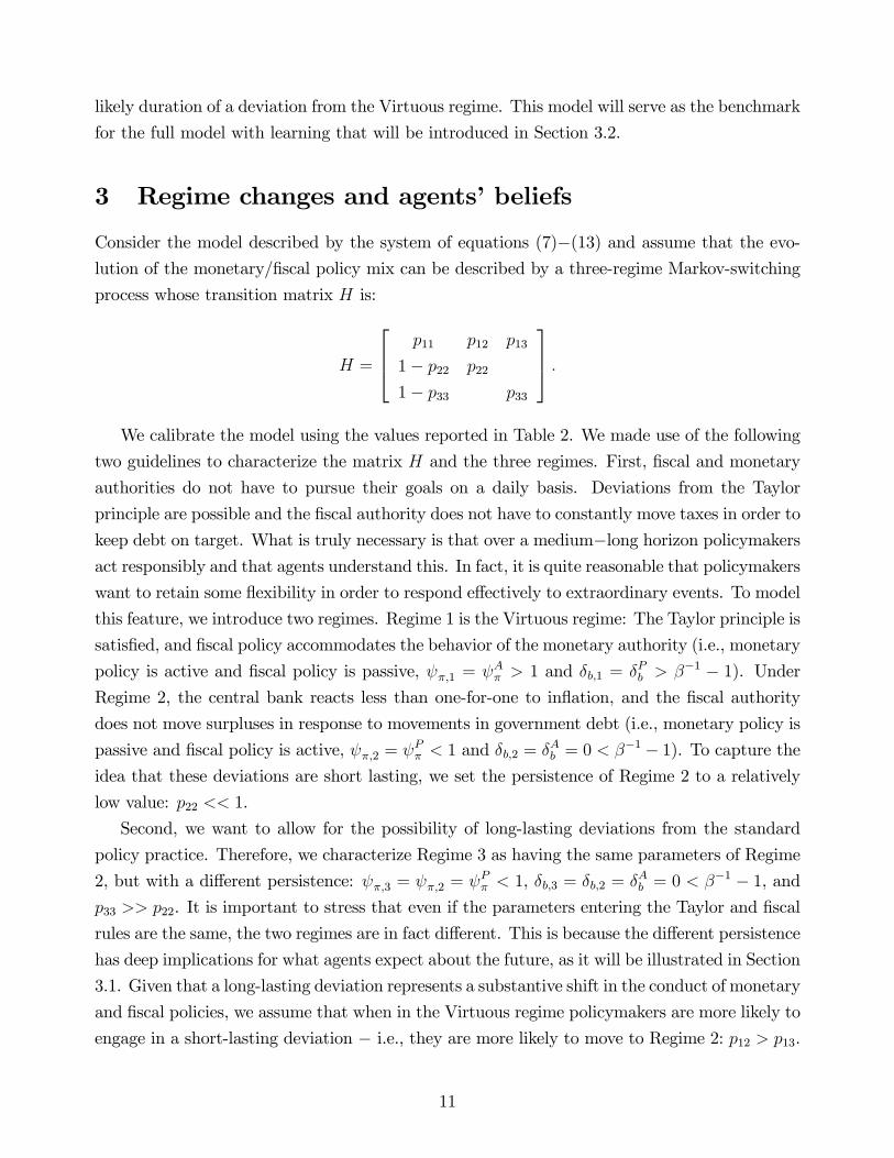
3 Regime changes and agents’beliefs

Consider the model described by the system of equations (7)−(13) and assume that the evo-lution of the monetary/fiscal policy mix can be described by a three-regime Markov-switching

process whose transition matrix H is:

H =

p11 p12 p13

1− p22 p22

1− p33 p33

.We calibrate the model using the values reported in Table 2. We made use of the following

two guidelines to characterize the matrix H and the three regimes. First, fiscal and monetary

authorities do not have to pursue their goals on a daily basis. Deviations from the Taylor

principle are possible and the fiscal authority does not have to constantly move taxes in order to

keep debt on target. What is truly necessary is that over a medium−long horizon policymakersact responsibly and that agents understand this. In fact, it is quite reasonable that policymakers

want to retain some flexibility in order to respond effectively to extraordinary events. To model

this feature, we introduce two regimes. Regime 1 is the Virtuous regime: The Taylor principle is

satisfied, and fiscal policy accommodates the behavior of the monetary authority (i.e., monetary

policy is active and fiscal policy is passive, ψπ,1 = ψAπ > 1 and δb,1 = δPb > β−1 − 1). Under

Regime 2, the central bank reacts less than one-for-one to inflation, and the fiscal authority

does not move surpluses in response to movements in government debt (i.e., monetary policy is

passive and fiscal policy is active, ψπ,2 = ψPπ < 1 and δb,2 = δAb = 0 < β−1 − 1). To capture the

idea that these deviations are short lasting, we set the persistence of Regime 2 to a relatively

low value: p22 << 1.

Second, we want to allow for the possibility of long-lasting deviations from the standard

policy practice. Therefore, we characterize Regime 3 as having the same parameters of Regime

2, but with a different persistence: ψπ,3 = ψπ,2 = ψPπ < 1, δb,3 = δb,2 = δAb = 0 < β−1 − 1, and

p33 >> p22. It is important to stress that even if the parameters entering the Taylor and fiscal

rules are the same, the two regimes are in fact different. This is because the different persistence

has deep implications for what agents expect about the future, as it will be illustrated in Section

3.1. Given that a long-lasting deviation represents a substantive shift in the conduct of monetary

and fiscal policies, we assume that when in the Virtuous regime policymakers are more likely to

engage in a short-lasting deviation − i.e., they are more likely to move to Regime 2: p12 > p13.

11

Parameter Value Parameter Value Parameter Value

ψAπ 0.80 ρs 0.90 100σR 0.20ψPπ 2.00 ρz 0.90 100σs 0.50ψAy 0.10 ρd 0.90 100σz 0.70

ψPy 0.10 b 1.00 100σd 0.40ρAR 0.75 κ 0.05 p11 95%ρPR 0.75 β 0.99 p12 4.95%δAb 0 p22 70%δPb 0.03 p33 99%

Table 2: Parameter choices of the DSGE parameters and of the transition matrix elements.

3.1 Perfect information

Before moving to the full model with learning, we will analyze the properties of the companion

model in which agents can observe all aspects of the economy, including the regime that is

in place at each point in time. When agents are aware of regime changes, standard solution

methods do not apply. Instead, we need to use one of the solution methods developed to handle

Markov-switching general equilibrium models. The solution algorithm employed in this paper

is based on the work of Farmer et al. (2010). The authors show that it is possible to reduce the

task of finding a Minimal State Variable solution to that of computing the roots of a quadratic

polynomial in several variables. When a solution exists, it can be characterized as a regime

switching vector-autoregression, of the kind studied by Hamilton (1989), Chib (1996), and Sims

and Zha (2006):

St = T (ξt, θ,H)St−1 +R (ξt, θ,H) εt. (14)

It is worth emphasizing that the law of motion of the DSGE states depends on the model

parameters (θ), the regime in place (ξt), and the probability of moving across regimes (H).

This means that what happens under regime i depends not only on the structural parameters

describing that particular regime, but also on what agents expect is going to happen under

alternative regimes and on how likely it is that a regime change will occur in the future.

The simplest way to understand the properties of the different regimes is to analyze the

impulse responses. We shall focus on a primary surplus shock to isolate the effects of fiscal

discipline. Under the assumption of nondistortionary taxation such a shock does not have any

impact on the macroeconomy if agents anticipate that policymakers will make the necessary

fiscal adjustments in order to repay the resulting increase in debt. Therefore, any detected

effect on the macroeconomy will be due to the lack of confidence that such adjustments will

be made. On the other hand, it is important to keep in mind that fiscal discipline affects the

propagation of all shocks. However, for the other shocks, we would need to separate the direct

impact of the shock from the effect due to the lack fiscal discipline (see Appendix B).

12

5 10 15 20 25 30 35 400

1

2

3

4

  GDP

5 10 15 20 25 30 35 40

2

4

6

8

Inflation

5 10 15 20 25 30 35 40

1

2

3

4

5

  FFR

5 10 15 20 25 30 35 40­5

0

5

10

  B/GDP

Virtuous (AM/PF)Short lasting deviationLong lasting deviation

Figure 1: Impulse responses to a two standard deviation primary deficit shock under perfect information. FFRstands for federal funds rate and B/GDP stands for public-debt-to-GDP ratio.

Figure 1 reports the impulse responses to a large primary deficit shock. The difference

between the long-lasting deviation and the other two regimes is particularly striking. Under

the Virtuous regime and the short-lasting deviation, we do not observe any effect on inflation

and output from this shock, whereas under the long-lasting deviation we observe a large and

persistent increase in inflation and an expansion in output. Under the Virtuous regime and the

short-lasting deviation, the debt-to-GDP ratio starts increasing slowly and steadily in response

to the increase in expenditure. The two paths differ only to the extent that under the Virtuous

regime, the government is adjusting primary surpluses in response to the increase in debt.

Under the long-lasting deviation, the debt-to-GDP ratio experiences a sudden drop, because of

the increases in inflation and GDP, followed by a smooth return to the steady state from below,

because of the increased level of expenditure and the slowdown in growth.

From these impulse responses, it should be clear that compared with a long-lasting deviation

from the Virtuous regime, a short-lasting deviation has very different implications. The inter-

esting fact here is that the behavior of the two authorities is identical across the two regimes.

However, the two regimes differ to the extent that they induce different expectations about the

policymakers’ future behavior. To illustrate this point, for each regime, Figure 2 reports the

one-step-ahead probability of observing a deviation from the Virtuous regime and the expected

number of consecutive deviations. When the economy is under the Virtuous regime, agents

are confident of staying there for a while, and the expected number of consecutive deviations

is very low. When under the short-lasting deviation, the one-step-ahead probability increases

13

Virtuous (AM/PF) Short lasting deviation Long lasting deviation0

0.2

0.4

0.6

0.8

1Probability of PM/AF for the next period

Virtuous (AM/PF) Short lasting deviation Long lasting deviation0

20

40

60

80

100Expected number of consecutive deviations

Figure 2: The two panels report respectively the one-step-ahead probability of a deviation from the Virtuousregime and the expected number of consecutive deviations under the different regimes under the assumptionthat agents have perfect information.

substantially, but the expected number of consecutive deviations is still very low (2.33). Finally

and most importantly, when policymakers engage in a long-lasting deviation, the number of ex-

pected consecutive periods of PM/AF policy mix increases substantially. Therefore, under the

short-lasting deviation, agents are confident that in the near future the government will run a

sequence of primary surpluses to balance the debt-to-GDP ratio. Instead, when a long -lasting

deviation occurs, agents are discouraged about a prompt return to the Virtuous regime. In this

case, the fiscal imbalance generated by the increase in primary deficits calls for an increase in

inflation. Given that the Taylor principle does not hold, the monetary authority accommodates

such a rise in inflation. This determines a drop in real interest rates, and output increases. High

inflation and the jump in output cause the drop in the debt-to-GDP ratio.

These results allow us to make a first important point: In a model with recurrent regime

changes, the policy mix is not enough to establish if a regime is Ricardian or not. Instead, the

persistence of the regime becomes a key ingredient given that it affects agents’expectations

about the conduct of fiscal and monetary policies in the medium-long run. When agents

are confident about a prompt return to the virtuous policy mix, a fiscal imbalance is not

inflationary even if policymakers do not immediately take care of it. Agents understand that

with high probability the necessary adjustments will occur in the future. Instead, when the

regime change is perceived to be too far into the future, inflation starts moving in response to

the fiscal imbalance.

3.2 Bayesian Learning

We are now ready to analyze the case in which agents cannot observe the regime they are in.

Let Ft be the agents’ information set. It is assumed that agents observe the history of theendogenous variables as well as the history of all shocks. However, agents do not observe the

14

history of regimes. Instead, they need to conduct Bayesian learning in order to infer the regime

that they are in. Regime changes are modeled as the three-regime Markov-switching process

described earlier. In this context, the transition matrix also reflects agents’priors about the

evolution of the monetary/fiscal policy mix.

Since agents know the history of endogenous variables and shocks, they can exactly infer

the policy mix that is in place at each point in time. However, while the Virtuous regime is

fully revealing, when the PM/AF mix is prevailing, agents do not know whether policymakers

are engaging in a short-lasting deviation or a long-lasting one. Agents have to learn the nature

of the deviation in order to form expectations over the endogenous variables of the economy.

An important result is then the following: Agents will grow more and more pessimistic about

moving back to the Virtuous regime, the longer the time spent under the alternative policy mix.

To see this, note that after having observed τ ≥ 1 consecutive deviations from the Virtuous

regime, agents believe that policymakers will keep deviating in the next period with the following

probability:4

prob {st+1 6= 1|Ft} =p22 (p12/p13) (p22/p33)τ−1 + p33

(p12/p13) (p22/p33)τ−1 + 1. (15)

The probability prob {st+1 6= 1|Ft} has a number of properties that shed light on the keyfeatures of the learning mechanism. Since p22 < p33, this probability is monotonically increasing

with respect to the number of last consecutive deviations τ . As the number of periods τ in

which the PM/AF policy mix has prevailed increases, agents become more and more pessimistic

about the odds of switching to the Virtuous regime in the next period. The reason is that as

policymakers keep deviating from the Virtuous regime, agents get increasingly convinced that

the two authorities are engaging in a long-lasting deviation (Regime 3) and are, therefore, more

unlikely to switch to the Virtuous regime (p22 < p33).

Furthermore, agents’pessimism admits an upper and lower bound. The intuition goes as

follows. For a given number of consecutive deviations τ , equation (15) shows that the probability

of observing another deviation next period will be a weighted average of p22 and p33. When

agents observe policymakers deviating from the Virtuous regime for the first time (τ = 1),

the weights are p12/ (p12 + p13) and p13/ (p12 + p13). This weighted average is the lower bound

for agents’ pessimism. The smaller the conditional probability of a long-lasting deviation,

p13/ (p12 + p13), the closer the lower bound will be to p22. As policymakers keep deviating,

agents get increasingly convinced that the economy has entered a long-lasting deviation, given

that under this regime long deviations are more likely. As the weight assigned to the long-lasting

deviation increases, the probability of observing an additional deviation increases, given that

p33 > p22. If policymakers deviate from the Virtuous regime for a very long time, agents will

4This result can be derived by applying Bayes’theorem and then combining the resulting probabilities withthe transition matrix H. See Bianchi and Melosi (2012b) for a detailed derivation.

15

0 5 10 15 20 25 300

0.2

0.4

0.6

0.8

1

τ

Beliefs: Regime probabilities

Virtuous (AM/PF)Short lasting deviationLong lasting deviation

0 5 10 15 20 25 300

0.2

0.4

0.6

0.8

1Probability PM/AF for next period

τ0 5 10 15 20 25 30

0

20

40

60

80

100

τ

Expected number of consecutive deviations

Figure 3: From left to right, the three panels describe, as a function of the number of consecutive deviationsτ , the evolution of agents’beliefs, the one-step-ahead probability of observing the PM/AF policy mix, and theexpected number of consecutive deviations from the Virtuous regime.

eventually become convinced of being in the long-lasting PM/AF regime, and the probability

of observing an additional deviation in the next period degenerates to the persistence of such

a regime:

limτ→∞

prob {st+1 6= 1|Ft} = p33. (16)

Hence, p33 is the upper bound for agents’pessimism. This implies that for each ε > 0, there

exists an integer τ ∗ such that:

p33 − prob {st+1 6= 1|τ = τ ∗} < ε, (17)

with the important result that for any τ > τ ∗, agents’beliefs can be effectively approximated

using the properties of the long-lasting PM/AF regime. In other words, agents cannot be more

pessimistic than when they are convinced of being in the long-lasting PM/AF regime.

These ideas are summarized in Figure 3. The first panel describes the evolution of agents’

beliefs as a function of the number of observed deviations from the Virtuous regime. The Virtu-

ous regime is fully revealing, therefore agents do not face any uncertainty.5 When agents observe

the first deviation, they are relatively confident that the prevailing regime is the short-lasting

PM/AF regime, given the assumption p12 > p13. However, as the number of deviations grows,

agents become more and more convinced that the economy has entered a long-lasting devia-

tion. Initially the probability attached to the long-lasting PM/AF regime increases slowly, but

it eventually accelerates as agents become less and less optimistic about a return to the Virtuous

regime. This has important implications on agents’expectations regarding the policymakers’

future behavior. The second and third panels of Figure 3 report the one-step-ahead probability

of observing the PM/AF policy mix and the expected number of consecutive deviations implied

5It is not hard to extend the model to allow for a short lasting and a long lasting AM/PF regime. Bianchiand Melosi (2012b) consider this case.

16

by the drift in beliefs. As agents observe more and more deviations, they become more and

more pessimistic and the expected number of consecutive deviations increases. As agents go

from being relatively optimistic to being relatively pessimistic, the expected number of con-

secutive deviations accelerates. Finally, as agents become convinced of being in a long-lasting

deviation, the expected number of consecutive deviations converges to the one prevailing under

the long-lasting PM/AF regime. This drift in beliefs about the future conduct of fiscal and

monetary policies has deep implications for the way shocks propagate through the economy.

However, we will first describe the solution method for the model with learning.

3.2.1 Solving the model with learning

It is very important to emphasize that the evolution of agents’beliefs about the future conduct

of fiscal and monetary policies plays a critical role in the Markov-switching model with learn-

ing. In fact, unlike the perfect-information model described in Section 3.1, the dynamics of

the endogenous variables in the model with learning cannot be fully captured by the three pol-

icy regimes. Instead, agents expect different dynamics for next period’s endogenous variables

depending on their beliefs about a return to the Virtuous regime.

Therefore, accounting for agents learning requires expanding the number of regimes and

redefining them as a combination between policymakers’behavior and agents’beliefs. Such new

regimes reflect different degrees of pessimism while agents are learning about the persistence

of the deviation from the Virtuous regime. Bianchi and Melosi (2012b) show that the Markov-

switching model with learning described previously can be recast in terms of an expanded set

of (τ ∗ + 1) > 3 new regimes, where τ ∗ > 0 is defined by the condition (17). The increased

number of regimes captures the degree of pessimism associated with observing deviations from

the Virtuous regime for τ = 1...τ ∗ periods. The τ ∗ + 1 regimes are given by

[(ξt = 1, τ t = 0) , (ξt 6= 1, τ t = 1) , (ξt 6= 1, τ t = 2) , ..., (ξt 6= 1, τ t = τ ∗)] ,

and the transition matrix H is defined as

H =

p11 p12 + p13 0 . . . 0 0

1− p12p22+p13p33p12+p13

0 p12p22+p13p33p12+p13

. . . 0 0

1− p12p222+p13p233p12p22+p13p33

0 0 . . . 0 0...

......

. . ....

...

1− p12p(τ∗−1)22 +p13p

(τ∗−1)33

p12p(τ∗−2)22 +p13p

(τ∗−2)33

0 0 0 0p12p

(τ∗−1)22 +p13p

(τ∗−1)33

p12p(τ∗−2)22 +p13p

(τ∗−2)33

1− p12pτ∗22+p13pτ

∗33

p12p(τ∗−1)22 +p13p

(τ∗−1)33

0 0 0 0p12pτ

∗22+p13pτ

∗33

p12p(τ∗−1)22 +p13p

(τ∗−1)33

.

Hence, one can recast the Markov-switching DSGE model with learning as a Markov-

17

switching Rational Expectations system, in which the regimes are redefined in terms of the

realized duration of the passive regimes, τ t. This result allows us to solve the model with regime

switches and learning by applying any of the methods developed to solve Markov-switching ra-

tional expectations models.

It is worth emphasizing that this way of recasting the learning process allows us to easily

model the behavior of agents that know that they do not know. In other words, agents are aware

of the fact that their beliefs will change in the future according to what they observe in the

economy. This represents a substantial difference with the anticipated utility approach, in which

agents form expectations without taking into account that their beliefs about the economy will

change over time. Furthermore, our approach differs from the one traditionally used in the

literature about learning in which agents form expectations according to a reduced form law

of motion that is updated recursively (for example, using discounted least squares regressions).

The advantage of adaptive learning is the extreme flexibility given that, at least in principle, no

restrictions need to be imposed on the type of parameter instability characterizing the model.

However, such flexibility does not come without a cost, given that agents are not really aware

of the model they live in, but only of the implied law of motion. Instead, in this paper, agents

fully understand the model and they are aware of the trade-offs that characterize it. However,

they are uncertain about the policymakers’future behavior, and this uncertainty has important

consequences for the law of motion of the economy.

3.2.2 Impulse responses

In order to understand the properties of the model, we will start illustrating how learning affects

the propagation of the shocks. Figure 4 contains impulse responses to a negative primary surplus

shock conditional on different starting values of the number of consecutive deviations, τ , under

the assumption that the PM/AF policy mix is in place over the entire horizon. The dark areas

correspond to large starting values for τ , while as the colors become lighter and lighter, the

starting number of deviations falls to 1 (i.e., at the time of the shock, agents observe the first

deviation from the Virtuous regime). We do not report here the response under the Virtuous

regime because this would look very similar to the one prevailing under perfect information, as

the regime is fully revealing.6

Before proceeding, it is worth stressing an important point. The assumption that the

PM/AF policy mix prevails over the entire horizon implies that the number of observed devi-

ations grows over time. This in turn determines a progressive change in the law of motion as

agents become more and more convinced that the economy has entered a long-lasting deviation.

The law of motion then stabilizes in the moment that agents become certain that they entered

6Nevertheless the impulse responses would not be identical because the uncertainty that prevails under thePM/AF regime also affects the law of motion under the Virtuous regime.

18

Figure 4: Impulse responses to a two standard deviation primary deficit shock under learning assuming thatthe PM/AF rule prevails over the relevant horizon. When moving from the light blue lines to the dark redlines, the time horizon increases from one year to five years. The impulse responses under the Virtuous regimeare very similar, although not identical, to the ones that prevail under perfect information, and are thereforeomitted. FFR stands for federal funds rate and B/GDP stands for public-debt-to-GDP ratio.

a long-lasting deviation (τ = τ ∗). The law of motion would change again if agents were to

observe a return to the Virtuous regime. This case will be analyzed in the Section 5.1.

Consider the case in which agents have observed a large number of consecutive deviations,

implying that agents are already convinced of being in the long-lasting PM/AF regime. As a

result, the impulse responses resemble very closely the ones implied by the same regime under

perfect information.7 Following the shock, inflation increases immediately, and then it slowly

declines. At the same time, the debt-to-GDP ratio experiences a large drop as a result of higher

growth and larger inflation, despite the increase in the primary deficit. As it was for the perfect

information case, these dynamics reflect the expectation that the government will not increase

future surpluses in order to cover the current deficits.

When the starting number of deviations is low, these effects are initially mitigated because

agents are confident about a prompt return to the Virtuous regime. During the first few periods,

inflation and GDP barely move, even if the current policymakers’behavior is still characterized

by the PM/AF policy mix. Consequently, we do not observe the drop in the debt-to-GDP

ratio, which instead starts increasing because of the primary deficits. However, as agents

7However, even when agents think that they are in the long-lasting PM/AF regime with probability one, thelaw of motion still slightly differs from the one implied by the model with perfect information because agents’expectations about the future reflect the additional uncertainty that derived from the learning mechanism.

19

Figure 5: The two sets of panels report the evolution of the endogenous variables and the correspondentexpected volatilities assuming a large primary surplus shock occurring at time 0 under the Virtuous regime.After five years, policymakers start deviating from the Virtuous regime (dashed vertical line). In the panels onthe right, when moving from the light blue lines to the dark red lines, the time horizon increases from one yearto five years. Expected volatilities are computed taking into account the possibility of regime changes. FFRstands for federal funds rate and B/GDP stands for public-debt-to-GDP ratio.

observe more and more deviations, their expectations start drifting, the law of motion evolves,

and the non-Ricardian dynamics start arising. Inflation starts to increase smoothly, then it

accelerates in the moment that agents become relatively pessimistic, and it finally reaches its

peak after approximately seven years. Symmetrically, real interest rates decline because the

Taylor principle does not hold, output starts growing, and the debt-to-GDP ratio falls.

4 Dormant shocks and Fiscal Virtue

As shown in Section 3.2.2, when learning is introduced in the model with regime changes, the

economy responds gradually to the shocks as agents update their beliefs about policymakers’

future behavior. The response to a fiscal shock is particularly interesting given that the learning

mechanism can substantially prolong its effects and move the peak of the responses further into

the future. In this section, we will analyze these features more in detail introducing the notion

of dormant shocks and characterizing their effects as a function of fiscal virtue.

20

4.1 Dormant shocks

Figure 5 considers a large negative shock to primary surpluses occurring at time 0 under the

Virtuous regime. After five years policymakers start deviating from the Virtuous regime and

they keep deviating for twenty years. The panels on the left report the impulse responses, while

the panels on the right contain the evolution of expected volatility at different horizons, from

1 year (light areas) to 5 years (dark areas). This measure of uncertainty is computed taking

into account the possibility of regime changes and the evolution of agents’beliefs, using the

methods described in Bianchi (2012a). For a variable Xt and an horizon T , it corresponds to√V (Xt+T |Ft).Notice that as long as the Virtuous regime prevails, the effects on inflation, output, and

federal funds rate (FFR) are basically undetectable as agents expect taxes to be raised in order

to repay the growing debt. However, as soon the policy mix changes, the learning process begins.

At this point an external observer focusing exclusively on the three standard macroeconomic

variables would be observing a slow moving increase in inflation and an acceleration in output

growth (and a positive output gap), along with a weak response of the FFR. All of these changes

would be without any apparent explanation, as no new shocks have occurred. Fiscal shocks

have therefore an interesting property in this environment: They can manifest themselves many

years after they occurred. In the meantime, they are just dormant shocks, given that they do

not have any apparent effect on the three standard macroeconomic variables. Notice that this

aspect makes them very hard to identify. If an econometrician were trying to understand the

causes of the slow-moving increase in inflation, he might be tempted to conclude that a change

in the target for inflation occurred. Alternatively, he might want to include fiscal variables

in order to estimate the model under the assumption that a non-Ricardian regime is in place.

However, if he happens to exclude the early years of the sample, he might have a very hard time

trying to recover any movement in the fiscal variables that could in fact explain the slow-moving

increase in inflation.

The increase in inflation is not the only effect of the changed economic environment. As

outlined in panels on the right of Figure 5, agents also face an increase in uncertainty. The

expected volatilities of the macroeconomic variables start increasing smoothly and reach a peak

in the moment that agents change from being relatively optimistic about a prompt return to

the Virtuous regime to being relatively pessimistic about this happening. These beliefs coincide

with the peak of uncertainty because agents attach similar probabilities to two very different

scenarios: (i) a large spur of inflation to cover the large debt and (ii) a return to the Virtuous

regime with a subsequent drop in inflation. This also explains why uncertainty is larger at

short horizons than at long horizons: In the long run, debt is expected to be closer to the

steady state, regardless of the path taken by policymakers, while in the short run, the large

21

stock of debt can have pervasive effects on the macroeconomy. Dormant shocks have therefore

another interesting effect: After many years they can cause an increase in the volatility of the

endogenous variables and consequently in agents’uncertainty. Once again, these effects are

dormant as long as the economy is under the Virtuous regime.

As agents become convinced that debt will be inflated away, the volatilities approach the

values associated with the long-lasting PM/AF regime. Under this regime, macroeconomic

uncertainty is larger than under the Virtuous regime for three reasons. First, given that the

Federal Reserve reacts less strongly to deviations of inflation from the target, any shock has

a larger direct impact on the dynamics of inflation. Second, any shock that moves the debt-

to-GDP ratio is also going to have an indirect impact on all the macroeconomic variables.

Third, the fiscal shocks that are dormant under the Virtuous regime, affect the macroeconomic

variables under the long-lasting PM/AF regime.

Based on these results, it should be clear that the Virtuous regime leads to a more stable

macroeconomic environment. Both inflation and output volatilities are smaller when policy-

makers refrain from long-lasting deviations from the Virtuous regime. However, it is worth

pointing out that this result might change in the moment more shocks are introduced in the

analysis. Bianchi and Melosi (2013) consider a particularly topical case: a large contraction in

aggregate demand that forces monetary policy to the zero lower bound. In this case, policy-

makers understand that a large recession and deflation can be avoided by abandoning fiscal

discipline, but this decision would also result in a sharp increase in macroeconomic instability

once out of the recession. On the other hand, announcing a period of fiscal austerity is detri-

mental in the short run, but it preserves macroeconomic stability in the long run. Therefore,

the moment that monetary policy is constrained, it is not clear anymore that sticking to fiscal

discipline is always preferable. We show that the policymakers’dilemma can be resolved by

committing to inflate away only the portion of debt resulting from the unusually large recession.

This determines an increase in short-run inflation expectations that mitigates the recession. At

the same time, long-run inflation expectations and uncertainty remain anchored as policymak-

ers’rules in response to other shocks are unchanged and the pre-crisis debt is still backed by

future fiscal adjustments.

In summarizing, an external observer monitoring the evolution of our hypothetical economy

would detect

a progressive increase in volatility and uncertainty, measured by expected volatility. At the

same time, she would observe an increase in inflation that seems to gain momentum over time.

Our external observer would probably conclude that the target for inflation has changed and

that the volatility of the exogenous shocks has increased.

22

100p13/ (p12 + p13) p22 τ ∗ 100p13/ (p12 + p13) p22 τ ∗

.04 0.70 40 1.00 .90 97

.20 0.70 36 1.00 .80 481.00 0.70 31 1.00 .70 315.00 0.70 26 1.00 .60 23

Table 3: Parameter values used in the study of dormant shocks. The persistences of the long-lasting PM/AFregime and of the AM/PF regime are fixed at .99 and .95, respectively.

4.2 Fiscal Virtue

The previous section has emphasized that dormant shocks can have effects many years after

they occurred. In this section, we will elaborate more on this point, trying to understand what

determines the lag between the time of the regime change and the peak of the inflation increase

that such a regime change triggers. We will show that two margins are important to understand

how quickly these events unfold. The first margin is represented by the relative probability of

entering a short-lasting deviation versus a long-lasting deviation and controls agents’a-priori

beliefs following a first deviation from the Virtuous regime. The second margin is given by the

relative persistence of the short- and long-lasting deviations and reflects agents’confidence in

ultimately responsible fiscal behavior.

Figure 6 considers the same exercise of the previous subsection for different values of the

ratio p13/ (p12 + p13). Recall that this ratio controls agents’a-priori beliefs of entering a long-

lasting versus a short-lasting deviation. In other words, it determines the probability attached

to the long-lasting deviation once agents observe the first realization of the PM/AF policy mix.

As this ratio declines, agents are a-priori more and more optimistic about the possibility of

facing only a temporary deviation from the Virtuous regime. Consequently, it takes longer for

agents to become convinced that they entered a long-lasting deviation. To capture this idea,

the different curves are labelled according to the implied τ ∗, i.e., the number of deviations

required for agents’beliefs to approximately coincide with the ones implied by the long-lasting

PM/AF regime. As explained in Section 3.2, this value represents an upper bound on agents’

pessimism about a prompt return to the Virtuous regime. The dotted line corresponds to the

benchmark case in which p13/ (p12 + p13) = 1% and τ ∗ = 31. Table 3 summarizes the mapping

for the other three curves.

As the ratio p13/ (p12 + p13) declines and τ ∗ increases, the peak of the inflation spur moves to

the right. When agents attach a conditional probability of .04% to the long-lasting regime, the

peak in inflation occurs thirteen years after the shock took place and eight years after the regime

change occurred. When instead agents are relatively pessimistic and p13/ (p12 + p13) = 5%,

the learning process is faster and the peak of inflation occurs only six years after the regime

change. Given that the ratio p13/ (p12 + p13) controls a-priori agents’beliefs, it is capturing the

23

20 40 60 80 1000

2

4

6

8

  GDP

20 40 60 80 100

5

10

15

20

25

30Inflation

20 40 60 80 100

5

10

15

20

25  FFR

20 40 60 80 100

10

20

30

40

  B/GDP

τ*=40τ*=36τ*=31τ*=26

Figure 6: The figure considers the effects of large a "dormant shock" to primary surplus for transition matricesthat differ according to the a-priori relative probability of a short-lasting deviation. The shock occurs at time 0,while the regime change occurs after 20 periods (red vertical bar). The different a-priori beliefs are captured bythe different periods necessary to convince agents that they entered a long-lasting deviation (τ∗). FFR standsfor federal funds rate and B/GDP stands for public-debt-to-GDP ratio.

20 40 60 80 1000

2

4

6

8

  GDP

20 40 60 80 100

5

10

15

20

25

Inflation

20 40 60 80 100

5

10

15

20

  FFR

20 40 60 80 100

10

20

30

40

  B/GDP

τ*=97

τ*=48

τ*=31

τ*=23

Figure 7: The figure considers the effects of a large "dormant shock" to primary surplus for transition matricesthat differ according to the relative persistence of the two PM/AF regimes. The shock occurs at time 0, while theregime change occurs after 20 periods (red vertical bar). The different values for the relative persistence of thedeviations are captured by the number of periods necessary to convince agents that they entered a long-lastingdeviation (τ∗). FFR stands for federal funds rate and B/GDP stands for public-debt-to-GDP ratio.

24

credibility of policymakers in agents’eyes. Agents’beliefs are likely to reflect some historical

evidence, in which case the matrix H would be pinned down by the relative frequencies of both

short-lasting and long-lasting deviations. Alternatively, we could imagine that agents form

subjective conjectures about how likely it is that the government will engage in a persistent

deviation from the Virtuous regime. In other words, agents could believe the occurrence of a

long-lasting deviation is more or less likely according to the policymakers’reputation. However,

no matter what agents’a-priori beliefs are, as long as agents update them according to what

they observe, the government cannot indefinitely avoid increasing taxes. In other words, no

matter how optimistic agents are, if the government deviates from the Virtuous regime for a

long period of time, eventually it will induce a change in expectations leading to an increase in

inflation and uncertainty. At the same time, if the government has been virtuous in the past,

it has probably built some reputation for avoiding long-lasting deviations. This translates into

a low value for p13/ (p12 + p13) and implies that policymakers can deviate for a longer period of

time without losing control of inflation expectations.

However, the a-priori relative probability of the two deviations is not the only margin that

affects the timing of the peak of inflation. The relative persistence of both the short- and

long-lasting deviations, p22/p33, is also important. When p22/p33 is low, the learning process

is faster as agents need only a few consecutive observations to conclude that they entered

a long-lasting deviation. In the limiting case in which the ratio is zero, agents just need

two consecutive deviations to conclude that they entered a long-lasting regime and that with

very high probability they will face a long series of PM/AF realizations. In contrast, when

p22/p33 is large, the learning process unfolds very slowly, and consequently the peak of inflation

occurs later (i.e., moves further to the right when plotted). Figure 7 illustrates this point.

The benchmark case is once again represented by the dotted line and the parameter choices are

summarized in Table 3. Notice that when p22/p33 = .9/.99 = 0.4762, the peak of inflation occurs

more than twenty years after the shock occurred and more than fifteen years after the regime

took place. Even in this case, the ratio can be interpreted as characterizing policymakers’

credibility, but for a different aspect. Specifically, agents might have different views about

what it means for a deviation to be short lasting. When, for a given persistence of the long-

lasting regime, this ratio increases, it means that agents remain confident about a return to

the Virtuous regime even after a relatively long sequence of deviations. Even in this case, the

relative persistence of the two regimes can be the result of some past evidence or determined by

an arbitrary conjecture about what it means for a regime to be short lasting. What matters is

that the persistences of the two regimes differ largely enough to make the distinction meaningful.

Furthermore, it is important to keep in mind that the characterization of one regime affects

the laws of motion of all the others. This implies that for a given set of parameters, there is

a limit to how large the ratio p22/p33 can be made without causing the short-lasting regime −

25

and possibly the Virtuous regime − to be inflationary.Fiscal Virtue can make the unfolding of the effects of dormant shocks smooth − a property

that seems appropriate to characterize inflation dynamics in economies in which policymakers

have strong reputation, such as the US economy. Countries for which the commitment to fiscal

responsibility is less clear are more likely to be subject to sudden shifts in agents’expectations

as agents need only a few deviations in order to decide that the economy has entered a long-

lasting deviation. This suggests an interesting interpretation of the different impulse responses

considered in this subsection: Following a shock of the same magnitude, countries with different

levels of fiscal virtue might experience similar levels of inflation as long a Virtuous regime is

in place. However, once they experience a deviation from the Virtuous regime, substantial

inflation differentials would arise as the speed of learning greatly differs across countries.

5 The History and Future of US Inflation

In this last part of the paper, we conduct a quantitative analysis based on a richer model aug-

mented with external habits, government purchases, inflation indexation to past inflation, and

a maturity structure for government debt, as well as a richer fiscal block in which government

expenditure and taxation are modeled separately. These features make the model more realistic

and allow us to calibrate the model using the estimates obtained by Bianchi and Ilut (2012).

Bianchi and Ilut (2012) estimate a DSGE model subject to a structural break from a PM/AF

regime to an AM/PF regime, and show that such break can account for the rise and fall of

US inflation and the change in the reduced form properties of the macroeconomy. Here we

expand the number of regimes to allow for a short-lasting and a long-lasting PM/AF regime

and introduce the learning mechanism while relying on the estimates to pin down the timing

of the switch to the Virtuous regime. A fully specified estimation exercise is beyond the scope

of this paper and, although feasible, poses some significant computational challenges that we

plan to take up in future research (Bianchi et al. (2012)). Appendix B contains an accurate de-

scription of the model, the parameter values, and impulse responses under perfect information

and learning.

5.1 A look at the past...

In the previous section, we introduced the concept of dormant shocks and showed how they

can propagate slowly over time and have the largest impact many years after they took place.

We will now put the theory to work showing how a few shocks, combined with the learning

mechanism, can go a long way in explaining the historical dynamics of inflation. Specifically,

we will show that three events could be central to understanding the run-up of inflation in the

26

’70s. The first event is a prolonged deviation from the Virtuous regime that lasted from the ’60s

until the appointment of Paul Volcker as Federal Reserve Chairman in 1979. The second event

is a large shock to the long-term component of government expenditure coinciding with the first

reference to the "Great Society" made by President Lyndon Johnson in May 1964. Following

Bianchi and Ilut (2012), we model this as a large and persistent increase in government transfers.

The third event is the tax cuts made by President Gerald Ford’s administration in the mid-’70s.

We choose a transition matrix in order to satisfy two criteria. First, we make the learning

process substantially slower, making the persistences of the short-lasting and long-lasting de-

viations more similar. Second, we make the ex ante conditional probability of a long-lasting

deviation very low. We then consider the following parameterization for the transition matrix:

H =

.9750 .0249 .0001

.0700 .9300

.0100 .9900

.The a-priori beliefs that agents assign to the policymakers having engaged in a long-lasting

deviation are very low (0.4%), and agents tolerate relatively long deviations as the ratio p22/p33

is relatively high. Therefore it takes around 37 years for agents to become convinced that they

entered a long-lasting deviation from the Virtuous regime (τ ∗ = 148).

We initialize the economy using the level of debt that was in place in 1955 and set all

the other variables to their respective steady states. We then assume a path for tax revenues

and total government expenditure that approximates the actual ones. These are reported in

the second and third panels of Figure 8. Given these paths and a sequence for policymakers’

behavior to be described later, we reconstruct a path for inflation. This is reported in the first

panel of Figure 8. We assume that policymakers started deviating during the late ’50s, and we

use the estimates of Bianchi and Ilut (2012) to pin down the return to the Virtuous regime,

occurring in mid-1980, a few quarters after the appointment of Volcker as Federal Reserve

Chairman (August 1979). These two events are marked by two vertical dashed lines, and the

gray area represents the period during which policymakers deviated from the Virtuous regime.

The two solid vertical lines mark the key shocks that are used to explain the increase in trend

inflation of the ’70s: The first reference made to the Great Society plans by President Johnson

and the Ford administration’s tax cuts. Finally, the dotted line in the fist panel represents the

path of inflation under the assumption that policymakers always follow the Virtuous regime.

Several aspects of this simulation are worth being mentioned. Following the Great Society

shock, inflation starts to rise, but very smoothly. In the short run, such low-frequency move-

ments are probably hard to detect. However, inflation keeps increasing, slowly but steadily,

even if in the simulated fiscal series there are no other shocks until the mid-’70s. By the time

27

1955 1960 1965 1970 1975 1980 1985 1990 1995 2000 20050

5

10In

flatio

n NonvirtuousActualThe theory

1955 1960 1965 1970 1975 1980 1985 1990 1995 2000 2005

16

18

20

Tax­

to­G

DP

1955 1960 1965 1970 1975 1980 1985 1990 1995 2000 2005

1618202224

Exp­

to­G

DP

Figure 8: The figure shows the results for a simulation meant to illustrate the properties of the model withlearning. Four events are key: 1) policymakers start deviating from the Virtuous regime in the late ’50s (firstdashed vertical line); 2) a large shock to the long-term component of expenditure assumed to coincide with thefirst reference to the Great Society made by President Johnson (first solid vertical line); 3) the Ford’s tax cut(second solid vertical line); and 4) the return to the Virtuous regime a few quarters after the appointment ofVolcker as Fed Chairman (second dashed vertical line). The solid lines correspond to the simulated data, thedashed line corresponds to the actual data, and the dotted line in the first panel shows the behavior of inflationunder the assumption that policymakers always follow the Virtuous regime.

the Ford tax cuts hit, inflation has already gained some momentum because of the acceleration

in agents’pessimism. Agents are now more pessimistic about the possibility of a quick return to

the Virtuous regime. Consequently, inflation rises faster following this second fiscal shock and

accelerates. It is worth pointing out that none of these events would have caused movements in

inflation if policymakers had always followed the Virtuous regime, as exemplified by the dotted

horizontal line in the first panel: All fiscal shocks are dormant when policymakers follow the

Virtuous regime. This inflationary spiral comes to an end with the appointment of Volcker as

Federal Reserve Chairman that can be regarded as a strong signal about the future conduct of

monetary and fiscal policies. The switch to the Virtuous regime determines a sudden drop in

inflation as agents’beliefs about policymakers’future behavior are subject to a drastic swing.

Fiscal shocks are now neutralized as agents revise their expectations about the way the debt

will be financed. As a result, all the movements in taxation and expenditure that follow the

return to the Virtuous regime have a negligible effect on inflation.

In summary, we have taken a historical perspective in this subsection to show how dormant

shocks can be used to explain low-frequency movements in the process for inflation. An impor-

tant lesson is that it might take a long time to see significant effects of these shocks on inflation,

which may give a false sense of security to policymakers. Finally, it is worth emphasizing that

28

the shocks by themselves would not have any impact on the macroeconomy. It is the interaction

between policymakers’behavior and the shocks that determines inflation dynamics.

5.2 ...to understand today and the future

Having shown that the model can account for the events of the past, we now use the same

calibration to analyze the current situation. Is the US economy heading toward a prolonged

period of high inflation? Should policymakers feel assured that long-term interest rates and

inflation expectations seem to be under control? In order to answer these questions, we will

compute forecasts conditional on two different scenarios about policymakers’future behavior.

For each forecast, we will use the state of the economy during the third quarter of 2009. For

each simulation, we compute the path for 5-year-ahead inflation expectations and the 5-year

bond yield. Both of them are computed taking into account the possibility of regime changes

using the methods developed in Bianchi (2012a).

Policymakers announce that the economy will be at the zero lower bound for one year. We

approximate such an announcement using a third regime that has the same characteristics of

the PM/AF regime, but for which the response to the output gap is set to zero. We believe

this is a convenient and potentially appropriate way to model the zero lower bound, given that

the Central Bank would probably react if inflation started rising substantially.

In the first scenario, the zero-lower-bound period is followed by the PM/AF policy mix, while

in the second case, the virtuous policy mix prevails. Furthermore, we assume that policymakers

do not make any announcement regarding the exit strategy, so agents do not know how the

economy will evolve after the zero-lower-bound period. Therefore, it is very important to specify

what agents expect is going to happen once the deviation is over. We assume that in the last

period of the announced deviation, the probability that agents attach to going back to the

Virtuous regime is equal to the one that would prevail if they had observed one year of PM/AF

policy. Notice that agents anticipate that this is the way they will think one year from the time

of the announcement.

Figure 9 reports the results. The first aspect that is worth noting is that long-term inflation

expectations are initially very well anchored regardless of policymakers’behavior. In a similar

fashion, the five-year bond yield is very low, in line with what is observed in the data. This is

because even if the PM/AF policy mix prevails, agents are initially optimistic about the prob-

ability of moving back to the virtuous combination. However, as time goes by, policymakers’

behavior starts making a difference. If policymakers insist in following the PM/AF combination,

agents get increasingly convinced that the economy has entered a long-lasting deviation from

the Virtuous regime. Accordingly, inflation and inflation expectations start drifting. Eventu-

ally inflation gets to levels that are comparable to the ones observed in the ’70s. If instead the

29

2010 2015 2020 2025 2030 20350

5

10

15Inflation

2010 2015 2020 2025 2030 203520

30

40

50

60Debt­to­GDP ratio

2010 2015 2020 2025 2030 20350

5

10

15Five­Year­Ahead Expected Inflation

2010 2015 2020 2025 2030 20350

5

10

15Five­Year Yield

VirtuousNonvirtuous

Figure 9: Conditional forecasts based on a transition matrix that implies high reputation of policymakers inpreventing large fluctuations in inflation. The zero lower bound is announced for one year. After that, twoscenarios are considered: always PM/AF or always AM/PF. In both cases, no announcement is made about theexit strategy from the zero lower bound. Five-year-ahead inflation expectations and the five-year bond yield arecomputed taking into account the possibility of regime changes.

virtuous policy mix is in place, this pattern is absent, as agents observe taxes being raised in

order to stabilize debt. In both cases, GDP growth experiences an acceleration in the short

run that reflects the fact that the economy is going back to the steady state. Interestingly, the

first spur of inflation that is associated with the recovery dies out very quickly, indicating that

an external observer could be induced to think that in both cases the central bank has still full

control of inflation dynamics. But this is just an illusion, as the run-up of inflation that follows

makes clear.

These conditional forecasts highlight the perils associated with trying to infer the risk of

high inflation looking at current inflation expectations or long-term interest rates. If it takes

time for agents to learn about the nature of the deviation that they are currently experiencing,

then their expectations are likely to be initially very well anchored. This is likely to be especially

true for an economy like that of the US that has experienced a prolonged period of monetary

dominated policy mix. In such an economy, the a-priori beliefs about the possibility of entering

a long-lasting deviation are arguably very low. Furthermore, it is worth pointing out that short-

lasting interventions that do not resolve the long-run problems of debt sustainability cannot be

interpreted as changes in policy mix. These are only shocks that do not move agents’beliefs

about the resolution of the long-term sustainability of government debt.

30

6 Conclusions

When agents are uncertain about the way debt will be stabilized the strict distinction between

Ricardian and non-Ricardian regimes typical of the literature on the fiscal theory of price level

breaks down. In its stead, a continuum of regimes reflecting agents’beliefs about the future

conduct of fiscal and monetary policies arises. As agents observe more and more deviations

from a Virtuous regime in which the central bank has full control of inflation, they become

increasingly convinced that debt will be inflated away. This implies that the law of motion

characterizing the economy evolves over time in response to what agents observe.

We introduced the notion of dormant shocks. These are shocks that move the debt-to-

GDP ratio and that have no effects on the macroeconomic variables when policymakers behave

according to a Virtuous regime. However, as policymakers start deviating from such a regime

and agents become more and more discouraged about the possibility of moving back to the

Virtuous regime, the effects of the dormant shocks arise, with a progressive increase in inflation

and uncertainty. Therefore, the model is able to generate a persistent and accelerating run-up

in inflation as relatively optimistic agents become more and more pessimistic.

We used the model to point out that currently low inflation expectations and low long-term

interest rates are likely to reflect the reputation US policymakers have built over the years.

This means that the true risk of inflation might be higher than what it appears and crucially

related to the way policymakers will behave in the future. If policymakers keep deviating

from the policies that have characterized their behavior in the three decades before the most

recent financial crisis, agents’pessimism about policymakers’ future behavior will eventually

accelerate, and so will inflation. At that point, only an immediate change in both fiscal and

monetary policies will be able to cut the inflationary spiral.

31

References

Atkeson, A., Chari, V. and Kehoe, P.: 2009, Sophisticated Monetary Policies, Quarterly Journal

of Economics 125(1), 47—89.Barro, R. J.: 1974, Are Government Bonds Net Wealth?, Journal of Political Economy

82(6), 1095—1117.Bassetto, M.: 2002, A game-theoretic view of the fiscal theory of the price level, Econometrica

70(6), 2167—2195.Benati, L.: 2008, Investigating inflation persistence across monetary regimes, The Quarterly

Journal of Economics 123(3), 1005—1060.Bianchi, F.: 2012a, Methods for Markov-switching Models, Duke University, working paper.

Bianchi, F.: 2012b, Regime Switches, Agents’Beliefs, and Post-World War II U.S. Macroeco-

nomic Dynamics, Review of Economic Studies, forthcoming.

Bianchi, F. and Ilut, C.: 2012, Monetary/Fiscal Policy Mix and Agents’Beliefs, Duke Univer-

sity, working paper.

Bianchi, F. and Melosi, L.: 2012a, Constrained Discretion and Central Bank Transparency,

working paper.

Bianchi, F. and Melosi, L.: 2012b, Modeling the Evolution of Public Expectations and Uncer-

tainty in General Equilibrium, Duke University, working paper.

Bianchi, F. and Melosi, L.: 2013, Escaping the Great Recession, working paper.

Bianchi, F., Melosi, L. and Ohanian, L.: 2012, Global Inflation, Duke University, working

paper.

Chib, S.: 1996, Calculating Posterior Distributions and Model Estimates in Markov Mixture

Models, Journal of Econometrics 75, 79—97.Clarida, R., Gali, J. and Gertler, M.: 2000, Monetary Policy Rules and Macroeconomic Stabil-

ity: Evidence and Some Theory, Quarterly Journal of Economics 115, 147—180.Cochrane, J. H.: 1998, A Frictionless Model of U.S. Inflation, in B. S. Bernanke and J. J.

Rotemberg (eds), NBERMacroeconomics Annual 1998, MIT Press, Cambridge, MA, pp. 323—

384.

Cochrane, J. H.: 2001, Long Term Debt and Optimal Policy in the Fiscal Theory of Price Level,

Econometrica 69, 69—116.Cochrane, J. H.: 2011, Understanding Policy in the Great Recession: Some Unpleasant Fiscal

Arithmetic, European Economic Review 55, 2—30.Cogley, T., Primiceri, G. and Sargent, T. J.: 2010, Inflation-Gap Persistence in the U.S, AEJ

Macroeconomics 2(1), 43—69.Cogley, T., Sargent, T. J. and Surico, P.: 2011, The Return of the Gibson Paradox. mimeo.

Coibion, O. and Gorodichenko, Y.: 2011, Monetary Policy, Trend Inflation, and the Great

32

Moderation: An Alternative Interpretation, American Economic Review 101(1), 341—370.Davig, T. and Doh, T.: 2008, Monetary Policy Regime Shifts and Inflation Persistence, Federal

Reserve Bank of Kansas City working paper.

Davig, T. and Leeper, E. M.: 2007, Generalizing the Taylor Principle, American Economic

Review 97(3), 607—635.Del Negro, M. and Eusepi, S.: 2011, Fitting Observed Inflation Expectations, Journal of Eco-

nomic Dynamics and Control 35(12), 2105—2131.Eusepi, S. and Preston, B.: 2010, The Maturity Structure of Debt, Monetary Policy and

Expectations Stabilization, Working Paper.

Farmer, R. E. A., Waggoner, D. and Zha, T.: 2010, Minimal State Variable Solutions to

Markov-Switching Rational Expectations Models, Federal Reserve Bank of Atlanta, mimeo.

Fernï£ ¡ndez-Villaverde, J., Rubio-Ramï£ ¡rez, J. F. and Guerrï£ ¡n-Quintana, P.: 2010, Fortune

or Virtue: Time-variant Volatilities versus Parameter Drifting in U.S. Data, Duke University

working paper.

Hall, G. J. and Sargent, T. J.: 2011, Interest Rate Risk and Other Determinants of Post-

WWII U.S. Government Debt/GDP Dynamics, American Economic Journal: Macroeco-

nomics 3(3), 192—214.Hamilton, J. D.: 1989, A New Approach to the Economic Analysis of Nonstationary Time

Series and the Business Cycle, Econometrica 57, 357—384.Ireland, P.: 2007, Changes in the Federal Reserve’s Inflation Target: Causes and Consequences.

Justiniano, A. and Primiceri, G.: 2008, The Time Varying Volatility of Macroeconomic Fluc-

tuations, American Economic Review 98(3), 604—41.Leeper, E. M.: 1991, Equilibria Under Active and Passive Monetary and Fiscal Policies, Journal

of Monetary Economics 27, 129—147.Liu, Z., Waggoner, D. and Zha, T.: 2011, Sources of the Great Moderation: A Regime-Switching

DSGE Approach, Quantitative Economics 2(2), 251—301.Lubik, T. and Schorfheide, F.: 2004, Testing for Indeterminacy: An Application to U.S. Mon-

etary Policy, American Economic Review 94(1), 190—217.Mankiw, N. G., Reis, R. and Wolfers, J.: 2004, Disagreement about Inflation Expectations,

NBER Macroeconomics Annual 2003, Volume 18, National Bureau of Economic Research,

Inc, pp. 209—270.

Melosi, L.: 2012, Signaling effects of monetary policy, Working Paper Series WP-2012-05,

Federal Reserve Bank of Chicago.

Melosi, L.: 2013, Estimating Models with Dispersed Information, American Economic Journal:

Macroeconomics, forthcoming.

Nimark, K.: 2008, Dynamic pricing and imperfect common knowledge, Journal of Monetary

Economics 55(8), 365—382.

33

Sargent, T. and Wallace, N.: 1981, Some Unpleasant Monetarist Arithmetic, Federal Reserve

Bank of Minneapolis Quarterly Review Fall, 1—17.Schmitt-Grohe, S. and Uribe, M.: 2000, Price level determinacy and monetary policy under a

balanced-budget requirement, Journal of Monetary Economics 45(1), 211—246.Schorfheide, F.: 2005, Learning and Monetary Policy Shifts, Review of Economic Dynamics

8(2), 392—419.Sims, C. A.: 1994, A Simple Model for Study of the Determination of the Price Level and the

Interaction of Monetary and Fiscal Policy, Economic Theory 4, 381—399.Sims, C. A.: 2011, Stepping on a Rake: The Role of Fiscal Policy in the Inflation of the 1970’s,

European Economic Review 55(1), 48—56.Sims, C. A. and Zha, T.: 2006, Were There Regime Switches in US Monetary Policy?, American

Economic Review 91(1), 54—81.Woodford, M.: 1994, Monetary Policy and Price Level Determinacy in a Cash-in-Advance

Economy, Economic Theory 4, 345—389.Woodford, M.: 1995, Price Level Determinacy without Control of a Monetary Aggregate,

Carnegie-Rochester Series of Public Policy 43, 1—46.Woodford, M.: 2001, Fiscal Requirements of Price Stability, Journal of Money, Credit, and

Banking 33, 669—728.Woodford, M.: 2003, Interest and prices: Foundations of a theory of monetary policy, Princeton

University Press, Princeton, New Jersey.

A Impulse responses for benchmark model

Figure 10 reports the impulse responses for the benchmark model under perfect information.

In the main text, we have already described how agents’expectations affect the propagation

of a fiscal shocks. Agents’expectations also affect the response of the economy to the other

shocks. The first row reports the responses to a monetary policy shock. Under all regimes,

the Federal Reserve retains the ability to generate a recession. However, under the long-lasting

PM/AF regime, inflation increases instead of declining. This "stepping on a rake" effect (Sims

(2011)) implies that the Central Bank loses its ability of controlling inflation the moment that

its actions are not adequately supported by the fiscal authority. Notice that the inflation

dynamics under the short-lasting deviation are very similar to the ones implied by the Virtuous

regime. This occurs despite the fact that the fiscal rule in place at the time of the shock

determines an increase in the debt-to-GDP ratio that could appear to be permanent to an

external observer. In the short run, given the presence of nominal rigidities, the increase in

the FFR determines an increase in the real interest that makes the cost of debt larger. Under

34

the short-lasting deviation, agents are confident that a return to the Virtuous regime will soon

occur. This is why the increase in debt is not inflationary. Under the long-lasting deviation

agents anticipate that the government will not increase primary surpluses in the near future

and inflation increases in order to stabilize debt. The Central Bank accommodates the increase

of inflation, and debt slowly declines because of negative real interest rates.8

The first row of Figure 11 illustrates that the stepping on a rake effect also arises when

introducing learning. When the initial number of deviations is small, in response to a monetary

policy shock inflation declines on impact and stays below the steady state for several periods.

However, as agents become aware of the possibility that the economy entered a long-lasting

deviation, inflation starts increasing and the stepping on a rake effect appears. If agents have

already observed a large number of deviations, the entire sequence of events occurs more quickly

and inflation immediately increases. These dynamics have two important implications. First,

when the initial number of deviations is small, a central bank might be initially induced to

believe that it is still able to control inflation, given that the stepping on a rake effect does

not immediately manifest itself. Second, as policymakers keep deviating and the ability of the

central bank to control inflation deteriorates, central bankers might erroneously be induced to

think that structural changes are occurring in the economy that are making the sacrifice ratio

less favorable.

B Extended model

In this appendix, we describe the model used in the quantitative analysis of Section 5. The

model is a simplified version of the one used in Bianchi and Ilut (2012).

B.1 Model description

Households. The representative household maximizes the following utility function:

E0

[∑∞s=0 β

seds[log(Cs − ΦCA

s−1

)− hs

]], (18)

subject to the budget constraint

PtCt + Pmt B

mt + P s

t Bst = PtWtht +Bs

t−1 + (1 + ρPmt )Bm

t−1 + PtDt −NTt,8The stepping on a rake effect is a robust finding, and it holds also in the richer model considered by Bianchi

and Ilut (2012). However, the short-run inflation dynamics can differ depending on the exact features of themodel.

35

1020

3040

­1

­0.50

Monetary Policy

  GD

P

1020

3040

­0.50

0.5

Infla

tion

1020

3040

0.51

1.5

  FFR

1020

3040

12  B

/GD

P

1020

3040

0.1

0.2

0.3

0.4

0.5

  Preference

1020

3040

0.1

0.2

0.3

0.4

0.5

1020

3040

0.1

0.2

0.3

1020

3040

­0.6

­0.4

­0.20

0.2

0.4

1020

3040

­0.8

­0.6

­0.4

­0.2

      TFP

1020

3040

0.2

0.4

0.6

0.81

1020

3040

0.2

0.4

0.6

1020

3040

0.2

0.4

0.6

0.8

1020

3040

024     Surplus

1020

3040

2468

1020

3040

12345

1020

3040

­50510Vi

rtuou

s (A

M/P

F)S

hort 

last

ing 

devi

atio

nLo

ng la

stin

g de

viat

ion

Figure10:Impulseresponsesforthebenchmarkmodelunderperfectinformation.FFRstandsforfederalfundsrateandB/GDPstandsforpublic-

debt-to-GDPratio.

36

Figure11:ImpulseresponsesforthebenchmarkmodelunderlearningassumingthatthePM/AFregimeprevailsovertherelevanthorizon.Movingfrom

thelight-bluetothedark-red,theinitialnumberofobserveddeviationsincreases.TheimpulseresponsesundertheVirtuousregimeareverysimilar,

althoughnotidentical,totheonesthatprevailunderperfectinformation.FFRstandsforfederalfundsrateandB/GDPstandsforpublic-debt-to-GDP

ratio.

37

where Dt stands for real dividends paid by the firms, Ct is consumption, Pt is the aggregate

price level, ht is hours, Wt is the real wage, NTt stands for net taxes, and CAt represents the

average level of consumption in the economy. The parameter Φ captures the degree of external

habit. The preference shock ds has a mean of zero and the following time series representation:

dt = ρddt−1 + σdεd,t. In line with Cochrane (2001), we recognize the importance of allowing

for a maturity structure of government debt. Longer maturities imply important fluctuations

in the return of bonds and consequently in the present value of debt. News about future

surpluses can then translate into smooth changes in inflation, as opposed to a discrete jump in

the current price level, even in absence of any additional friction. Hall and Sargent (2011) show

that revaluation effects explain a significant fraction of the fluctuations of the debt-to-GDP

ratio. Following Eusepi and Preston (2010) and Woodford (2001), we assume that there are

two types of government bonds: one-period government debt, Bst , in zero net supply with price

P st and a more general portfolio of government debt, B

mt , in non zero net supply with price P

mt .

The former debt instrument satisfies P st = R−1

t . The latter debt instrument has the payment

structure ρT−(t+1) for T > t and 0 < ρ < 1. The value of such an instrument issued in period

t in any future period t + j is Pm−jt+j = ρjPm

t+j. The asset can be interpreted as a portfolio of

infinitely many bonds, with weights along the maturity structure given by ρT−(t+1). Varying

the parameter ρ varies the average maturity of debt.

Firms. Each of the monopolistically competitive firms faces a downward-sloping demandcurve:

Yt(j) = (Pt(j)/Pt)−1/υ Yt, (19)

where the parameter 1/υ is the elasticity of substitution between two differentiated goods. The

firms take as given the general price level, Pt, and the level of real activity, Yt. Whenever a

firm changes its price, it faces quadratic adjustment costs represented by an output loss:

ACt(j) = .5ϕ (Pt(j)/Pt−1(j)− Πt−1)2 Yt(j)Pt(j)/Pt, (20)

where Πt = Pt/Pt−1 is gross inflation at time t.

The firm chooses the price Pt(j) to maximize the present value of future profits:

Et [∑∞

s=tQs ([Ps(j)/Ps]Ys(j)−Wshs (j)− ACs(j))] ,

where Qs is the marginal value of a unit of the consumption good. Labor is the only input

in a linear production function, Yt(j) = Atht (j), where total factor productivity At evolves

according to an exogenous process: ln (At/At−1) = γ + at, at = ρaat−1 + σaεa,t, εa,t ∼ N (0, 1) .

Government. Imposing the restriction that one-period debt is in zero net supply, the flow

38

budget constraint of the federal government is given by

Pmt B

mt = Bm

t−1 (1 + ρPmt )− Tt + Et + TPt,

where Pmt B

mt is the market value of debt and Tt and Et represent federal tax revenues and

federal expenditures, respectively. The term TPt is a shock that is meant to capture a series

of features that are not explicitly modeled here, such as changes in the maturity structure and

the term premium. This shock is necessary to avoid stochastic singularity when estimating the

model given that we treat debt, taxes, and expenditures as observables.9 We rewrite the federal

government budget constraint in terms of debt-to-GDP ratio bmt = (Pmt B

mt ) / (PtYt):

bmt =(bmt−1R

mt−1,t

)/ (ΠtYt/Yt−1)− τ t + et + tpt,

where all the variables are now expressed as a fraction of GDP and Rmt−1,t = (1 + ρPm

t ) /Pmt−1 is

the realized return of the maturity bond. We assume tpt = ρtptpt−1 + σtpεtp,t, εtp,t ∼ N (0, 1) .

The (linearized) federal government expenditure as a fraction of GDP, et, is the sum of a

short-term component eSt and a long-term component eLt (et = eLt + eSt ):10

eLt = ρeL eLt−1 + σeLεeL,t, εeL,t ∼ N (0, 1) ,

eSt = ρeS eSt−1 + (1− ρeS)φy (yt − ynt ) + σeSεeS ,t, εeS ,t ∼ N (0, 1) .

The long-term component is assumed to be completely exogenous, and it is meant to capture

the large programs that arise as the result of a political process that is not modeled here. Con-

sistently with this interpretation, we assume that this component of government expenditure

is known one year ahead. Instead, the short-term component is meant to capture the response

of government expenditure to the business cycle and responds to the (log-linearized) output

gap (yt − ynt ), where ynt is the natural output, i.e., the level of output that would prevail under

flexible prices. Notice that government expenditure is the sum of federal transfers and good

purchases.

The federal and local/state governments buy a fraction ζt of total output, equally divided

among the J different goods. We define gt = 1/(1 − ζt), and we assume that gt = ln(gt/g∗)

9An alternative approach consists of excluding one of the fiscal components, for example, the series for debt.Our results are robust to this alternative specification. We also considered an alternative specification in whichan observation error for the series of debt is included and the term premium shock is eliminated. The resultsare virtually identical.10In what follows, for a given variable Xt, xt ≡ log ((Xt/At) / (X/A)) represents the percentage deviation of

a detrended variable from its own steady stade. For all the variables normalized with respect to GDP (debt,expenditure, and taxes), xt denotes a linear deviation (xt = Xt−X), while for all the other variables, xt denotesa percentage deviation (xt = log (Xt/X)). This distinction avoids having the percentage change of a percentage.

39

follows the process

gt = ρggt−1 +(1− ρg

)φeS e

St−1 + σgεg,t, εg,t ∼ N (0, 1) . (21)

Before proceeding it is important to point out that we assume that local and state govern-

ments participate in purchasing goods and that they are supposed to run a balanced budget.

Therefore, changes in net taxes at the state level are neutral as agents understand that they will

be offset by future changes in the opposite direction. We believe this is a reasonable assumption

as it is quite unlikely that in the United States local governments can exercise influence on the

conduct of monetary policy.

Monetary and Fiscal Rules. The Central Bank moves the FFR according to the rule:

Rt

R=

(Rt−1

R

)ρR(ξt)[(

Πt

Π

)ψπ(ξt)(YtY nt

)ψy(ξt)](1−ρR(ξt))

σReεR,t , εR,t ∼ N (0, 1) , (22)

where R is the steady-state (gross) nominal interest rate, Y nt is natural output, and Π is gross

steady-state inflation. The federal fiscal authority moves taxes according to the rule

τ t = ρτ (ξt) τ t−1 + (1− ρτ (ξt))[δb (ξt) b

mt−1 + δeet

]+ δy

(yt−1 − ynt−1

)+ στετ ,t, ετ ,t ∼ N (0, 1) ,

(23)

where τ t denotes (linearized) tax revenues with respect to GDP.

In equations (6) and (5), ξt is an unobserved state variable capturing the monetary/fiscal

policy combination that is in place at time t. The unobserved state takes on a finite number of

values j = 1, ...,m and follows a Markov chain that evolves according to a transition matrix H.

The targets for inflation and debt are assumed to be constant over time.11 What changes is the

strength with which the government tries to pursue its goals, not the goals themselves. This is

in line with the idea that policymakers might find high inflation or high debt acceptable under

some circumstances (perhaps in order to preserve output stability) but not desirable in itself.

B.2 The linearized model

Once the model is solved, the variables can be rescaled in order to induce stationarity. The

model is then linearized with respect to taxes, government expenditure, and debt, whereas

it is log-linearized with respect to all the other variables. We obtain the following system of

equations:

11See Ireland (2007), Liu et al. (2011), and Schorfheide (2005) for models that allow for a time-varying target.

40

1. IS curve:

(1 + Φγ−1

)yt = gt

(1 + Φγ−1 − ρg

)+ Φγ−1 (yt−1 − gt−1)

−(1− Φγ−1

) [Rt − Et [πt+1] + (ρd − 1) dt

]+ Et [yt+1] +

(ρa − Φγ−1

)at;

2. Phillips curve:

(1 + β) πt = κ(1− Φγ−1

)−1 [yt − gt − Φγ−1 [yt−1 − gt−1 − at]

]+ κµt + πt−1 + βEt [πt+1] ,

where κ ≡ 1−υυϕΠ2 ;

3. Monetary policy rule:

Rt = ρRRt−1 + (1− ρR)[ψππt + ψy (yt − ynt )

]+ σRεR,t;

4. Total Government purchases:

gt = ρggt−1 +(1− ρg

)φeS e

St−1 + σgεg,t;

5. Fiscal rule:

τ t = ρτ (ξt) τ t−1 + (1− ρτ (ξt))[δb (ξt) b

mt−1 + δeet

]+ δy

(yt−1 − ynt−1

)+ στετ ,t;

6. Debt:

bmt = β−1bmt−1 + bmβ−1(Rmt−1,t − yt + yt−1 − at − πt

)− τ t + eSt + eLt + tpt;

7. Return long term bond:

Rmt,t+1 = R−1ρPm

t+1 − Pmt ;

8. No arbitrage:

Rt = Et

[Rmt,t+1

];

9. Expenditure, short-term component:

eSt = ρeS eSt−1 + (1− ρeS)φy (yt − ynt ) + σeSεeS ,t;

41

Parameter Value Parameter Value Parameter Valueψπ (ξt = 1) 0.6244 δe 0.7045 100σR 0.1972ψπ (ξt = 2) 2.3522 δy 0.0869 100στ 0.4564ψy (ξt = 1) 0.3716 ρe 0.9950 100σa 0.6518ψy (ξt = 2) 0.1527 Φ 0.7779 100σe 0.3653ρR (ξt = 1) 0.8480 ρa 0.4540 100σd 6.9498ρR (ξt = 2) 0.8132 ρd 0.6125δτ ,b (ξt = 1) 0 κ 0.0128 p11 0.9000δτ ,b (ξt = 2) 0.0327 100 ln (γ) 0.4896 p12 0.0990ρτ (ξt = 1) 0.7306 b∗ 0.9644 p22 0.7000ρτ (ξt = 2) 0.8921 τ ∗ 0.1846 p33 0.9900

Table 4: Parameter choices of the DSGE parameters and of the transition matrix diagonal elements based onBianchi and Ilut (2011).

10. Expenditure, long-term component (assumed to be known four periods in advance):

eLt = ρeL eLt−1 + σeLεeL,t;

11. Term premium/maturity shock:

tpt = ρtptpt−1 + σtpεtp,t;

12. Technology:

at = ρaat−1 + σaεa,t;

13. Demand shock:

dt = ρddt−1 + σdεd,t.

B.3 Impulse responses

Figures 12 and 13 report the impulse responses for the extended model under perfect information

and under learning, respectively.

42

1020

3040

­0.1

5­0

.1­0

.050

  MP

∆G

DP

1020

3040

­0.10

0.1

   In

fl

1020

3040

00.

20.

40.

6

   FF

R

1020

3040

­0.500.

511.

5  

 B/G

DP

1020

3040

­0.8

­0.6

­0.4

­0.20

   P

m

1020

3040

0

0.1

0.2

 TECH

1020

3040

­0.1

5­0

.1­0

.050

1020

3040

­0.1

­0.0

500.

05

1020

3040

­1.5­1

­0.50

1020

3040

0

0.2

0.4

1020

3040

­0.0

8­0

.06

­0.0

4­0

.020

 TAX

1020

3040

­0.4

­0.2

1020

3040

­0.4

­0.2

1020

3040

­4­20

1020

3040

0.2

0.4

0.6

0.81

1.2

1020

3040

00.

020.

040.

06

 DEM

1020

3040

­0.0

20

0.02

1020

3040

­0.0

200.

020.

04

1020

3040

­0.2

­0.10

1020

3040

­0.0

50

0.05

1020

3040

00.

020.

040.

060.

08

LTEXP

1020

3040

0.1

0.2

0.3

0.4

0.5

1020

3040

0.2

0.4

1020

3040

­202

1020

3040

­1.5­1

­0.5

AM

/PF

SL 

PM

/AF

LL P

M/A

F

Figure12:Impulseresponsesfortheextendedmodelunderperfectinformation.

MP,TECH,TAX,DEM,andLTEXPstandformonetarypolicy,

technology,tax,demand,andlongterm

expenditureshock,respectively.FFRandB/GDPstandforFederalFundsrateandpublic-debt-to-GDPratio.

43

Figure13:ImpulseresponsesfortheextendedmodelunderlearningassumingthatthePM/AFregimeprevailsovertherelevanthorizon.Whenmoving

from

thelightbluelinestothedarkredlines,theinitialnumberofobserveddeviationsincreases.TheimpulseresponsesundertheAM/PFarevery

similar,althoughnotidentical,totheonesthatprevailunderperfectinformation.MP,TECH,TAX,DEM,andLTEXPstandformonetarypolicy,

technology,tax,demand,andlongterm

expenditureshock,respectively.FFRandB/GDPstandforFederalFundsrateandpublic-debt-to-GDPratio.

44