PIC for Accelerator Science

James Amundson Fermilab

For the ComPASS Collaboration

ComPASS

ComPASS ComPASS

The ComPASS Collaboration

• To enable scientific discovery in HEP, high-fidelity simulations are necessary to develop new designs, concepts and technologies for particle accelerators

• Under SciDAC3, ComPASS is developing and deploying state-of-the-art accelerator modeling tools that utilize – the most advanced algorithms on

the latest most powerful supercomputers

– cutting-edge non-linear parameter optimization and uncertainty quantification methods.

Community Project for Accelerator Science and Simulation

ComPASS ComPASS

This talk

• PIC methods • Two closely related application areas

– Beam Dynamics – Advanced Accelerators – Require tracking particles interacting with fields

calculated on grids • HEP (Fermilab, UCLA) working with ASCR

[FastMATH (LBNL), Fermilab, UCLA] • Only one sub-topic of the ComPASS project. For a

comprehensive overview, see SciDAC PI 2012 talk by Panagiotis Spentzouris

ComPASS ComPASS

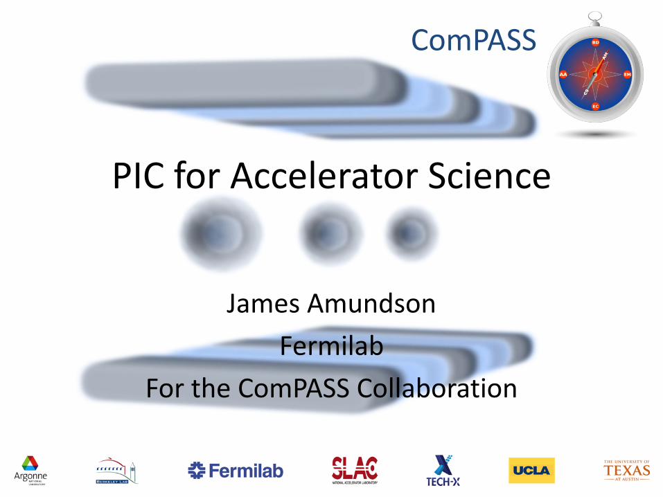
Application areas: Beam Dynamics and Advanced Accelerators

• Beam Dynamics – Existing and planned accelerators – Complex devices that need to be

simulated for long times • Accelerators can have 1000s of elements • 1000s to 1000000s of revolutions

• Advanced Accelerators

– Next-generation acceleration technology • Huge field gradients promise dramatically

smaller/cheaper accelerators • Two types

– Plasma-wakefield acceleration (PWFA) – Laser-wakefield acceleration (LWFA)

– Complex fields, short time scales

ComPASS ComPASS

Application areas: Beam Dynamics and Advanced Accelerators

• Beam Dynamics – Internal + External fields

• External field calculations trivially parallelizable

– All P, no IC • Internal field calculations

same as AA – Minimal bunch/field

structure

• Advanced Accelerators – Pure PIC – Complicated

bunch/field structure

ComPASS ComPASS

Scaling

Scaling achievements to date in beam dynamics and

advanced accelerators

ComPASS ComPASS

Beam Dynamics: scaling achievements

• Synergia – Single- and multiple-bunch simulations

Single-bunch strong scaling from 16 to 16,384 cores 32x32x1024 grid, 105M particles

Weak scaling from 1M to 256M particles 128 to 32,768 cores

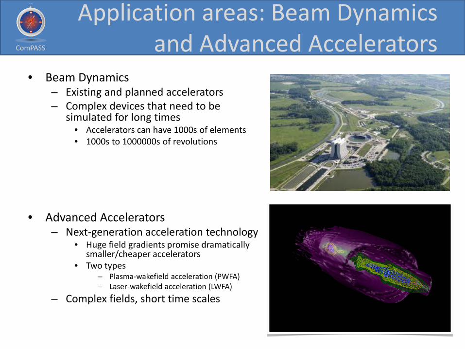
Weak scaling from 64 to 1024 bunches 8192 to 131,072 cores Up to over 1010

particles

Scaling results on ALCF machines: Mira (BG/Q) and

Intrepid (BG/P)

ComPASS ComPASS

Synergia in production

ComPASS ComPASS

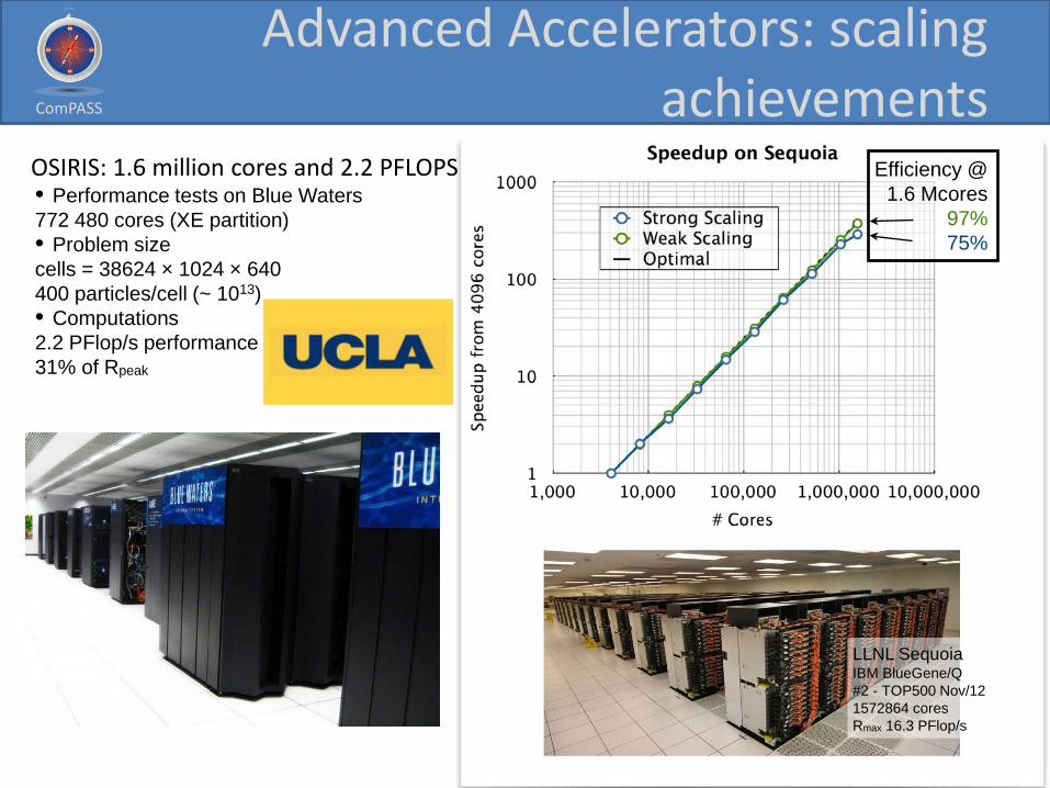
LLNL Sequoia IBM BlueGene/Q #2 - TOP500 Nov/12 1572864 cores Rmax 16.3 PFlop/s

Efficiency @ 1.6 Mcores

97% 75%

OSIRIS: 1.6 million cores and 2.2 PFLOPS • Performance tests on Blue Waters 772 480 cores (XE partition) • Problem size cells = 38624 × 1024 × 640 400 particles/cell (~ 1013) • Computations 2.2 PFlop/s performance 31% of Rpeak

Advanced Accelerators: scaling achievements

ComPASS ComPASS

How we achieved scaling in Synergia

• Challenge: beam dynamics simulations are big problems requiring many small solves – Typically 643 – 1283 (2e5 – 2e6 degrees of freedom)

• Compare with 2.5e10 in OSIRIS scaling benchmark – Will never scale to 1e6 cores – Need to do many time steps (1e5 to 1e8)

• All “scaling” advice we received was with respect to grid size – Included decomposing particles by grid location – In beam dynamics, external fields can cause particles to move

over many grid cells in a single step • Communication required to maintain decomposition and load

balancing – Point-to-point communication – Complicated for both programmer and end user

» Change in physical parameters can change communication time by x100

ComPASS ComPASS

Synergia: first scaling advances

• Eliminate particle decomposition – Requires collective communication

• But not point-to-point • Big machines are optimized for collectives

– Simpler for programmer and end-user – Helps a little, but leads to…

• Breakthrough: Redundant field solves (communication avoidance) – Field solves are a fixed-size problem

• Scale to 1/nth of problem

ComPASS ComPASS

Synergia: communication avoidance

• Communication avoidance – Used to have two global communications

• collect charge density • broadcast calculated field (x3 dimensions)

– Fields are now limited to a small set of cores, so the latter is greatly reduced

• Allows scaling in number of particles – Not limited by the scalability of the field solves – Excellent (i.e., easy) scaling

ComPASS ComPASS

Synergia: large numbers of particles

• Many reasons to use more particles and/or more complex particle calculations – Accuracy of long-term simulations

• Statistical errors in field calculations become more important as the number of steps increases

– Detailed external field calculations • Significant feature of Synergia • Application-dependent

– Accurate calculation of small losses • High-intensity accelerators require very small losses

– Calculating 1e-5 losses at 1% requires 1e9 particles

ComPASS ComPASS

Synergia: new scaling opportunities • Multi-bunch wakefield

calculations – Excellent scaling

• Bunch-to-bunch communications scale as O(1)

– Also relatively small

– Already discovered multi-bunch instabilities in the Fermilab Booster

• Not accessible with “fake” multi-bunch

• Parallel sub-jobs

– Parameter scans, optimization – Part of our workflow system

• Makes it easier on end user • Avoids error-prone end user

editing of job scripts

ComPASS ComPASS

Synergia: scaling final

• Scaling advances are the product of many factors – Redundant solves (communication avoidance) (x4-

x10) • Every simulation

– Large statistics (x1-x1000) • Some simulations

– Multiple bunches (x1-x1000) • Some simulations

– Parallel sub-jobs (x1 – x100) • Some simulations

• Product can be huge (x4 – x1e8)

ComPASS ComPASS

Emerging technology research

GPUs and multicore architectures

ComPASS ComPASS

Emerging technology research

• GPUs and Multicore • Shared memory is back! • Some things get easier, some harder

• Charge deposition in shared memory systems is the key challenge

• Multi-level parallelism very compatible with our communication avoidance approach

ComPASS ComPASS

Advanced Accelerator simulations on GPUs and multicore

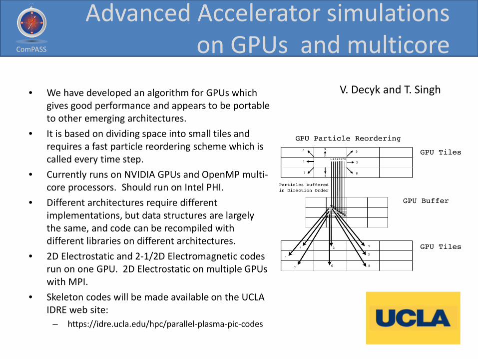
• We have developed an algorithm for GPUs which gives good performance and appears to be portable to other emerging architectures.

• It is based on dividing space into small tiles and requires a fast particle reordering scheme which is called every time step.

• Currently runs on NVIDIA GPUs and OpenMP multi-core processors. Should run on Intel PHI.

• Different architectures require different implementations, but data structures are largely the same, and code can be recompiled with different libraries on different architectures.

• 2D Electrostatic and 2-1/2D Electromagnetic codes run on one GPU. 2D Electrostatic on multiple GPUs with MPI.

• Skeleton codes will be made available on the UCLA IDRE web site:

– https://idre.ucla.edu/hpc/parallel-plasma-pic-codes

V. Decyk and T. Singh

ComPASS ComPASS

AA: GPU-accelerated results • Benchmark with 2048x2048 grid, 150,994,944 particles, 36 particles/cell • optimal block size = 128, optimal tile size = 16x16. Single precision • GPU algorithm also implemented in OpenMP

CPU:Inteli7 GPU:M2090 OpenMP(12 cores)

Push 22.1 ns 0.532 ns 1.678 ns

Deposit 8.5 ns 0.227 ns 0.818 ns

Reorder 0.4 ns 0.115 ns 0.113 ns

Total Particle 31.0 ns 0.874 ns 2.608 ns

CPU:Inteli7 GPU:M2090 OpenMP (12 cores)

Push 66.5 ns 0.426 ns 5.645 ns

Deposit 36.7 ns 0.918 ns 3.362 ns

Reorder 0.4 ns 0.698 ns 0.056 ns

Total Particle 103.6 ns 2.042 ns 9.062 ns

• Electrostatic • mx=16, my=16, dt=0.1 • Total speedup was

about 35 compared to 1 CPU, and about 3 compared to 12 CPUs.

• Electromagnetic • mx=16, my=16,

dt=0.04, c/vth=10 • Total speedup was

about 51 compared to 1 CPU, and about 4 compared to 12 CPUs.

ComPASS ComPASS

Beam dynamics simulations on GPUs and multicore

• Nearly the same problem as in AA – Particles can move many cells in between steps

• Optimal decomposition/deposition schemes differ

Q. Lu, JFA

ComPASS ComPASS

Charge deposition in shared memory

One macro particle contributes up to 8 grid cells in a 3D regular grid

Collaborative updating in shared memory needs proper synchronization or critical region protection

CUDA

• No mutex, no lock, no global sync

• Atomic add – yes, but not for double precision types

OpenMP

• #pragma omp critical • #pragma omp atomic

• Both very slow

ComPASS ComPASS

Charge deposition in shared memory – solution 1

Each thread has a duplicated spatial grid, and charges will be deposited to that grid only

T 1 T 2 T 3 T 4 T n

Parallel reduction

CUDA • Concurrency be an issue for GPU • Memory bottleneck at final reduction

OpenMP • Works well at 4 or 8 threads • Scales poorly at higher thread counts

Parallel reduction among all n-copy of spatial grids

ComPASS ComPASS

Charge deposition in shared memory – solution 2

Sort particles into their corresponding cells using parallel bucket sort

Deposit based on color-coded cells in an interleaved pattern (red-black)

List of particles Grid cells

CUDA • High thread concurrency • Good scalability, even the overhead shows

reasonable scaling • No memory bottleneck • Better data locality at pushing particles

OpenMP • Non-trivial sorting overhead for low

thread counts

ComPASS ComPASS

Charge deposition in shared memory – solution 2

Grid level interleaving Iteration_1 Iteration_2

Iteration_3 Iteration_4

ComPASS ComPASS

Charge deposition in shared memory – solution 2

Step 1: Deposit at x=thread_id

Step 2: Deposit at x=thread_id+1

Sync-barrier

Thread level interleaving

ComPASS ComPASS

BD: GPU and multicore results

OpenMP results GPU results

Scheme 1

Scheme 2

Node boundary

ComPASS ComPASS

Advanced algorithms: two-grid schemes for PIC

• Using the same domain decomposition for the field solve grids and for the particle deposition results in load imbalance.

• For simulations for which the are a

large number of particles per grid cell, we perform field solves and field-particle transfers with different grids.

• Particles handled with sorted space-

filling curve, transfers to local “covering set” grids (distributed sorting can be hard!)

• The transfer between the two sets of

grids is done efficiently, since the amount of field data is small relative to the particle data.

ComPASS ComPASS

Advanced algorithms: method of local corrections

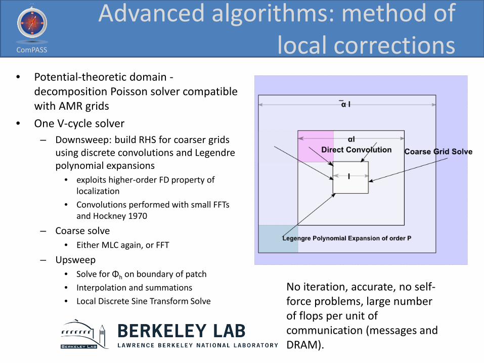
• Potential-theoretic domain -decomposition Poisson solver compatible with AMR grids

• One V-cycle solver – Downsweep: build RHS for coarser grids

using discrete convolutions and Legendre polynomial expansions

• exploits higher-order FD property of localization

• Convolutions performed with small FFTs and Hockney 1970

– Coarse solve • Either MLC again, or FFT

– Upsweep • Solve for Φh on boundary of patch • Interpolation and summations • Local Discrete Sine Transform Solve

No iteration, accurate, no self-force problems, large number of flops per unit of communication (messages and DRAM).

ComPASS ComPASS

Conclusions

• PIC methods for accelerators now scale to the size of the biggest available machines – Multiple factors make this practical in production

runs

• Working implementation of GPU/multicore-optimized algorithms

• Advanced algorithmic research underway