Phytoplankton  Composition  

Under  Resource  Limitations  

     

 42  EC  

(20th  Feb  2013  –  30th  September  2014)    

Emma  Greenwell  :  10407995  MSc  Biological  sciences:    

Limnology  and  oceanography  Supervisor:  Amanda  Burson  Examiner:  Maayke  Stomp  

IBED,  UvA  March  28th  2014  

     

  2  

Table  of  Contents  

I.  Abstract  ..............................................................................................................  3  

II.  Introduction  .......................................................................................................  4  2.1  Nutrient  limitations  ...................................................................................................................................  4  2.1.1  previous  research  ....................................................................................................................................  5  2.1.2  Management  ..............................................................................................................................................  5  

2.2  Competition  ...................................................................................................................................................  7  2.2.1  nutrient  limitations  ................................................................................................................................  7  2.2.2  light  limitation  ..........................................................................................................................................  8  

2.3  Aims  ..................................................................................................................................................................  9  

III.  Materials  and  methods  ...................................................................................  10  3.1  Analysis  ........................................................................................................................................................  12  3.2  Dissolved  inorganic  nutrients  ............................................................................................................  14  3.2.1  DIN  ..............................................................................................................................................................  14  3.2.2  DIP  ...............................................................................................................................................................  14  3.2.3  DISi  ..............................................................................................................................................................  14  

IV.  Results  ............................................................................................................  15  4.  1  Low  Nitrogen:  Low  Phosphate  Chemostat  ..................................................................................  17  4.1.1  Phytoplankton  population  ................................................................................................................  17  4.1.2  Abiotic  parameters  ..............................................................................................................................  17  

4.  2  Mid-­‐Nitrate:  Mid-­‐Phosphate  Chemostat  .......................................................................................  17  4.2.1  Phytoplankton  population  ................................................................................................................  17  4.2.2  Abiotic  parameters  ..............................................................................................................................  17  

4.3  High  Nitrate:  High  Phosphate  Chemostat  .....................................................................................  18  4.3.1  Phytoplankton  population  ................................................................................................................  18  4.3.2  Abiotic  parameters  ..............................................................................................................................  18  

4.4  Low  Nitrate:  High  Phosphate  Chemostat  ......................................................................................  20  4.4.1  Phytoplankton  population  ................................................................................................................  20  4.4.2  Abiotic  parameters  ..............................................................................................................................  21  

4.5  High  Nitrate:  Low  Phosphate  Chemostat  ......................................................................................  21  4.5.1  Phytoplankton  population  ................................................................................................................  21  4.5.2  Abiotic  parameters  ..............................................................................................................................  21  

4.6  Mid-­‐Nitrate:  High  Phosphate  Chemostat  .......................................................................................  23  4.6.1  Phytoplankton  population  ................................................................................................................  23  4.6.2  Abiotic  factors  ........................................................................................................................................  24  

4.7  High  Nitrate:  Mid-­‐Phosphate  chemostat  .......................................................................................  24  4.7.1  Phytoplankton  population  ................................................................................................................  24  4.7.2  Abiotic  parameters  ..............................................................................................................................  24  

4.9  All  chemostats:  Summary  .....................................................................................................................  25  4.9.1  Beginning  .................................................................................................................................................  25  4.9.2  final  states  ................................................................................................................................................  26  

V.  Discussion  ........................................................................................................  28  5.1  Species  and  their  limiting  nutrients  ................................................................................................  28  5.1.1  ‘pushing’  nutrient  environments  ....................................................................................................  29  

5.2  Species  dominance  (beginning  and  end  state)  ...........................................................................  30  5.3  Summary  of  end  state  species  ............................................................................................................  33  5.3  Limitations  ..................................................................................................................................................  34  5.4  conclusion  ...................................................................................................................................................  35  

VI.  Reference  list  ..................................................................................................  35  

  3  

 

I.  Abstract    Phytoplankton   are   the   basis   of   the   pelagic   food  web,   therefore   any  alterations   in   their   composition   can  affect  higher   trophic   levels  and  the   economic   value   of   marine   products.   Marine   waters   have  traditionally  been  known  to  be  nitrogen  (N)  limited  while  freshwater  was   phosphorous   (P)   limited.   De-­‐eutrophication   measures   have  begun   to   alter   this   standard   of   thought   as   the   reduction   of  phosphorus   entering   coastal   seas   has   been   much   more   successful  when  compared  to  nitrogen.  Thus,  the  CHARLET  project  is  looking  at  the  recent  change  from  nitrogen  to  phosphorous  limitation  in  coastal  seas.   Does   this   change   in   nutrient   limitation   alter   phytoplankton  composition  (through  competition)  in  a  positive  or  negative  way,  or  not   at   all?   Competition   for   resources   can   occur   when   the   ratio   of  availability   of   N   to   P   is   skewed,   or   due   to   light   limitation   when  nutrient   loads   are   replete.   To   test   this   nutrient-­‐ratio   hypothesis,  North  Sea  inoculum  was  gathered  and  placed  into  chemostats  with  7  different   nutrient   ratios   and   varying   loads   (LowN:LowP,  LowN:HighP,   HighN:HighP,   HighN:MidP,   HighN:LowP,   MidN:MidP  and   MidN:HighP).   Lugols   and   flow   cytometry   samples   were   taken  consistently   for   3   months   for   further   species   identification   and  species   counts.   Results   showed   that   diatoms   (Nitschia   agnita   and  Nitschia   pusilla)  were   the   best   competitors   in   low   to   mid   nutrient  loads   of   16:1   N:P   ,   the   diatom   N.   pusilla   was   best   suited   to  phosphorous   limited   conditions   (LowN:LowP   and   HighN:LowP),  Chlorella   sp.   was   the   best   competitor   for   low   light   situations  while  potentially   nitrogen   fixing   cyanobacteria   “2”  was   able   to   utilize   the  extremely  low  nitrogen  levels.  In  conclusion  changes  in  nutrient  ratio  and   load   do   allow   predictions   of   phytoplankton   composition  however  only  at  group  level  (green  algae,  cyanobacteria,  diatom  etc.).        

  4  

II.  Introduction    Autotrophic   phytoplankton   are   the   base   of   the   entire   pelagic   food  web.  Therefore  changes  in  phytoplankton  dominance  can  disrupt  the  functions   interacting  within   the  aquatic  ecosystem  (Henriksen  et  al.  2002).    Shifts  in  phytoplankton  community  composition  can  produce  changes  in  higher  trophic  species  (Tilman  et  al.  1986,  Phillipart  et  al.  2007  and  Navarro  and  Lobbam  2009).  Further  shown  by  Beaugrand  et   al.     in   2003   where   long   term   changes   in   Atlantic   cod   (Gadus  morhua   L.)  were   shown   to   be   not   only   a   result   of   over   fishing,   but  also   by   changes   and   fluctuations   of   phytoplankton   species   and  abundance.   The   economic   value   of   plankton/marine   products   can  also   suffer,   such   as   the   seaweed   (Nori)   aquaculture   in   Japan  which  has   been   negatively   impacted   by   undesired   phytoplankton   blooms  (Imai   et   al.   2006).     Understanding   the   key   factors   responsible   for  changes   in   phytoplankton   communities   is   of   interest   to   many  different  stake  holders.        

2.1  Nutrient  limitations    As  a  driving   factor   in  phytoplankton  productivity  nutrients,   such  as  nitrogen   and   phosphorus,   are   extensively   investigated,   especially  with   respect   to   which   is   limiting   growth.   Nutrient   limitation  continuously   shapes   phytoplankton   communities   as   shown   by  Philippart  et  al.  (2000)   in  a  strong   longitudinal  high-­‐resolution  time  series   study   of   20   years   (1974-­‐1994).     A   causal   relationship   was  found   between   phytoplankton   and   nutrient   concentrations   on   the  Wadden   Sea.   It   showed   drastic   changes   in   phytoplankton  communities  that  coincided  with  changes  in  nutrient  concentrations.  Weekly  sampling  (1962-­‐1984)  in  the  German  Bight  showed  increases  in  N  concentration  reducing  the  Si:N  ratio  to  <0.1  resulting  in  a  shift  from   a   high   diatom   abundance   to   high   flagellates   (Radach   et   al.,  1990).   Nutrient   limitation   has   been   the   focus   of   many  marine   and  freshwater  research  over  the  years,  and  rightly  so.  The  importance  of  understanding   phytoplankton   composition   in   relation   to   nutrient  uptake  and  availability  is  paramount  as  this  may  allow  for  prediction  

  5  

of   toxic   algal   blooms,   among   other   management   related   issues  (Brauer  et  al.  2012).    

2.1.1  previous  research    Research  has  repeatedly  shown  marine  environments  to  be  nitrogen  limited  (Hecky  1988;  Elser  et  al  2007  and  Phillipart  et  al.  2007)  due  to  strong  de-­‐nitrification,  low  amounts  of  N-­‐fixing  cyanobacteria  and  high   rates   of   SO4   reduction   (through   microbes)   that   consequently  makes  it  harder  for  Fe  ions  to  isolate  phosphorous  which  is  bound  to  the   sea   floor   (Ekholm  2008).  This  makes  phosphorous  unattainable  in  the  water  column  rendering  it  the  limiting  nutrient.  Phosphorous,  on   the   other   hand,   is   the   most   common   limiting   nutrient   in  freshwater   environments   (Hecky   1988   and   Elser   et   al   2007).    However,   recent   studies   have   shown   phosphorous   to   be   the   main  limiting  nutrient  in  regards  to  phytoplankton  primary  production  in  the   western   Wadden   Sea   (Philippart   et   al.,   2007   and   Ly   et   al.,   in  prep.).   While   this   is   contradictory   to   the   previous   theories   as   the  Wadden  Sea  is  a  highly  dynamic  water  body  (Van  Raaphorst  and  De  Jonge,  2004)  with  high   input  of   freshwater   from  surface   runoff   and  nearby   estuaries   (Graneli   and   Sundback   1985).   This,   as   with   some  other   coastal   waters   in   close   proximity   with   large   rivers   and  estuaries,   hint   that   the   high   freshwater   input   in   coastal   areas   can  result   in   areas   of   phosphorous   limitation,   even   in   marine  environments.  In  some  cases,  such  as  the  southern  area  of  the  North  Sea,  nutrient   input   from   freshwater   can  account   for  around  75%  of  the  water  body  (Skogen  et  al.,  2004).  

2.1.2  Management    This  decrease  in  phosphorus  is  not  strictly  due  to  naturally  occurring  P-­‐limitations  in  the  freshwater  inputs,  but  rather  is  in  part  a  result  of  de-­‐eutrophication  efforts.    Due  to  increased  occurrences  of  toxic  algal  blooms  pre-­‐1987  (Cadee  1986),  during  a  international  conference  in  early   1980’s   European   countries   developed   a   target   to   reduce  amounts   of   nutrients   in   their   major   rivers   (mainly   nitrogen   and  phosphorous)  and  therefor  entering  the  coastal  zones.  Phosphorous,  due   to   municipal   improvements,   was   decreased   by   50%   (target  

  6  

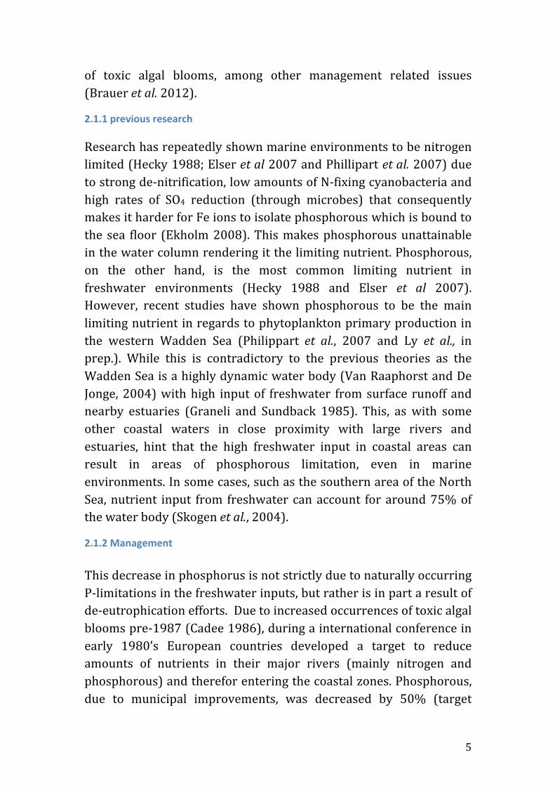
achieved)  while  nitrogen  was  decreased  by   the   lesser  30%  (Skogen  et  al.  2004).  Figure  1  shows  the  phosphorous  decrease  This  uneven  decrease  in  the  N  and  P  loads  in  freshwater  inputs  have  also  brought  a   decrease   in   the   retention  of   Si,  which   then   also   flushes   to   coastal  zones,   increasing   the   coastal   Si   load.   The   increase   in   Si   is   key   to  producing   increased   diatom  blooms   in  Dutch   coastal  waters  within  the   North   Sea   (Prins   et   al.   2012).   Some   might   say   this   could   be  beneficially,   as   it   is   known   that   diatoms   carry   a   greater   capacity   to  take   up   carbon   (Prins   et   al.  2012   and   Smetacek   1999)   providing   a  greater  energy  transfer  towards  higher  trophic  levels  (Litchman  et  al.  2009   and   Prins   et   al.   2012)   or   alternatively   transporting   carbon  towards  the  ocean  floor  when  sinking  (Smetacek  1999).  On  the  other  hand   there   is   a   choice   to   be   made   whether   this   increased   energy  transfer  outweighs  the  occurrences  of  harmful  diatom  blooms  (Prins  et  al.  2012).  Different  outcomes  have  been  recorded,  some  showing  a  decrease   in   biomass   within   already   low   phosphorous   water  environments   (Skogen   et   al.   2004),   while   others   have   documented  that   even   with   the   decreases   in   phosphorous   and   nitrogen,   net  increases   in   both   concentrations   can   be   seen   over   the   last   century  (Cloern,  2001).                      

Still  there  have  been  recent  cases  of  harmful  algal  blooms  (Philippart  et  al.  2007;  Schindler  2006;  Anderson  2002  and  Cloern  2001),  which  have   researchers   even   more   invested   in   the   ‘nutrient   load  hypothesis/nutrient   resource   ratio’  put   forward  by  Tilman   in  1986.  This  theory  states  that  total  nutrient  load  may  not  be  the  only  factor  

Figure  1:  Decreasing  phosphorous  concentrations  from  sea’s  around  the  Netherlands.  Decreases  in  phosphorus  can  be  seen  in  1985  (implementation  of  phosphorus  reduction  (Ecomare,  undated)  

  7  

in   species   competition  and   therefore   composition,  but   that  nutrient  ratio   also   is   important   in   determining   species   composition   (Tilman  1986,  Miller  et  al.  2005).  There  is  much  and  equal  evidence  for  both  ratio   (e.g.  Vrede  et  al.,   2009)  and  absolute  amount   (e.g.  Downing  et  al.,   2001)   being   the   predecessor   of   composition   with   absolute  amount  being  more  important  in  eutrophic  conditions  (Brauer  et  al.,  2012).   A   few   have   proposed   the   theory   that   nutrient   enrichment  causes   the   competition   for   nutrients   to   shift   to   light   (Brauer   et   al.,  2012;  Passarge  et  al.,  2006;  Kilham  1986  and  Huisman  et  al.,  2002).      

2.2  Competition    In   order   to   understand   why   certain   species   are   dominant   over  others,   competition  experiments  and  models  are   implemented.  Best  described   by   Brauer   et   al.   (2012)   when   looking   at   competition  between  two  species:  If  both  species  are  limited  by  the  same  nutrient  then   the   species   with   the   lowest   R*   value   for   said   nutrient   will  outcompete   the   other   (seen   in   figure   2A).   R*   value   refers   to   the  minimum  amount  of  the  resource  needed  to  produce  positive  growth  (Miller  et  al.  2005).  Limiting  nutrients  are  taken  up  faster  than  others  allowing   species   to   push   their   environment   to   favor   their   limiting  conditions.  However,  when   two   species   are   competing   for   different  limiting  nutrients,  a  trade  off  can  exist  where  stable  coexistence  and  alternative  stables  states  may  arise  (seen  in  figure  2B)  (Litchman  et  al.  2007).    

2.2.1  nutrient  limitations    Here  species  A  has  the  lowest  R*  for  phosphorous  while  species  B  has  the   lowest  R*   for  nitrogen.  From  this  we  can  say   that  species  A   is  a  good   competitor   for   phosphorous   and   species   B   for   nitrogen.  However   the   nutrient   supply   point   and   consumption   vectors  determine  the  species  composition.  When  the  initial  nutrient  supply  point   is  within   the  consumption  vectors  stable  coexistence  between  both  species  is  possible.  When  the  nutrient  supply  point  is  outside  of  these  vectors,  both  species  may  be  present  although  consumption  of  their   nutrients   will   soon   push   the   initial   conditions   towards   a  

  8  

limitation   (by  quick   consumption  of   limiting  nutrient)   (represented  by   bold   arrows   in   figure   2B)   that   ultimately   eliminates   one   of   the  species.  Alternative   stables   states,   although  difficult   to   prove   in   the  field,   is   still   a   possible   outcome   of   competition.   Seen   in   figure   2C,  alternative   stable   states   are  determined  by   the   initial   abundance  of  species  A  and  B  and  the  time  of  the  initial  nutrient  supply  (Brauer  et  al.  2012).   If   it   is  able   to  monopolize   the   limiting  resource,   the  more  abundant  species  will  exclude  others.                                            

2.2.2  light  limitation    When  nutrients  are  plentiful,   the  composition  of  phytoplankton  will  not   be   dictated   by   competition   for   nutrients   but   rather   a   third  resource  becomes  limiting;  light.  At  a  certain  point  species  will  start  

A   B  

C   D  

Figure   2:   competition  models   for   competitive  exclusion   (A),   co-­‐existence   (B),   alternative   stable  states  (C)  and  addition  of   light  (D).  Green  dotted   line  represents  consumption  vectors,  blue  and  red  isocline  represents  species  A  and  B,  orange  circles  represent  initial  nutrient  supply  points  and  bold  arrows  represent  ‘pushing  the  environment’  (made  by  author,  based  off  of  Tilmans  work).    

  9  

to   self-­‐shade   each   other   and   therefor   cause   light   limitation  (Anderson   et   al.   2002).   When   light   limitation   is   added   into  competition  models  (figure  2D)  we  can  see  that  a  third  species  (C)  is  present.  This  is  because  for  species  C,  light  is  the  limiting  resource  for  which  it  is  the  best  competitor.    Alternatively  it  could  be  that  species  A  for  example  also  happened  to  be  the  best  competitor  for  light  and  therefore  would  outcompete  in  both  environments,  this  is  a  situation  where  there  is  no  tradeoff.        

2.3  Aims    This  study  was  carried  out  alongside  the  CHARLET  project  (CHanges  in  Resource  Limitation  and  Energy  Transfer).  The  project  started   in  January  2011  and  is  focusing  their  research  on  three  main  criteria:  1.  The  recent  changes  from  nitrogen  to  phosphorous  limitation  in  the  coastal  North  Sea.    2.  Whether  these  changes  can  affect  the  phytoplankton  composition?  3.Whether   these   changes   create   positive   or   negative   impacts   in   the  aquatic   environment.   Positive   referring   to   an   increase   of   the  nutritional   value   of   phytoplankton   thus   increasing   the   energy   to  higher  trophic  levels,  or  negative  leading  to  unhealthy  cells  prone  to  viral   lysis   and   therefore   energy   remaining   trapped   within   the  microbial  loop  (NWO).    This   study   focuses  on   criterion  number  2;  will   changes   in  N:P   ratio  impact   the  phytoplankton  community  of   the  North  Sea?  To  address  this,   we   worked   with   chemostats,   which   are   used   as   a   model   of   a  marine   ecosystem   (Groove   2000)   to   investigate   phytoplankton  composition  changes.    Using  an   inoculum   taken   from   the  North  Sea  during  an  early  spring  cruise  and  growing  under  different  N:P  ratios  and   loads   we   can   see   how   these   impact   community   composition.    Applying   the   theory   of   Brauer   et   al.   (2012),   Tilman   (1985),   and  Huisman   &  Weissing   (1994,   1995)   to   the   observed   results   we   can  begin  to  understand  the  potential   impact  the  increasing  N:P  ratio  of  the  North  Sea  will  have  on  its  phytoplankton  composition.  

  10  

III.  Materials  and  methods    The   research   cruise   was   carried  out  during  15-­‐22nd  March  2013  on  the  North  Sea.  Niskin  bottles  were  attached   to   a   conductivity,  temperature  and  depth  device  and  2.5   L   of   seawater   was   collected  from   a   depth   of   7   meters.   The  water  was   then  used   to   rinse  and  fill  a  container.  This  was  repeated  for   seven   different   stations   along   the   transect   (figure   3).   At   each  station,  water  collected  was  filtered  through  a  200-­‐micrometer  sieve  to  eliminate  zooplankton.  After  which,  CO2  gas  was  bubbled  through  the   filtered   seawater   for   30   minutes   to   eliminate   any   leftover  zooplankton.   All   seawater   samples   were   then   mixed   together   in  equal   proportions,   to   account   for   preconditioning,   and   transported  back  in  one  10  L  carboy  to  the  lab  and  stored  at  4oc.    In  the  laboratory,  seven  chemostats  were  constructed  as  in  Huisman  et  al.  2002  (Figure  4)  using  full-­‐spectra  white  fluorescent  bulbs  as  the  light   source.   Magnetic   stirrers   were   placed   in   each   chemostat   to  avoid   accumulation   of   sticky   and   heavy   species.   Chemostats   were  

positioned   for   an   average   Iin   (light  entering   the   chemostat)   of   40μmol  photons   m-­‐2   s-­‐1  and   flow-­‐through   rate  was   adjusted   to   allow   for   a   0.20   day-­‐1  dilution  period.      Seawater   inoculum   was   added   to   fill  half   the   volume   of   the   chemostats   to  which   nutrient   medium   (Table   1A)  with   seven   different   nitrogen  

(NaNO3):Phosphorous  (K2HPO4•3H2O)  ratios  (Figure  1B)  was  added  through   peristaltic   pumps   set   to   a   steady   flow   rate.   Overflow   was  passed   into  sterile  waste   tanks.  Required  volume  of  sample  per  day  

9

The CHARLET-2 cruise 2012 We studied during late spring the biology of plankton (with a major focus on phytoplankton) in the North Sea, along a transect from coastal waters to central North Sea water. This cruise was undertaken as part of larger integrated study with the main merit of assessing the production, composition and losses of phytoplankton in order to determine the limiting factors for phytoplankton growth in the North Sea and study how these limiting factors affect the food quality and species composition of the phytoplankton. This is the first of four cruises, during spring and summer. The cruise track is shown in Figure 2. Station details in Table 1 and the participant and crew list in Table 2.

Fig. 2. Cruise track CHARLET-1, summer 2011. This cruise was longer in duration. During the present CHARLET-2 cruise, May 2012, we have sampled from south to north stations 13, 11, 10, 8, 7, 4, 2, and 1.

Figure  3:  satellite  image  of  stations    (transect).  Water  samples  taken  from  station  1,  2,  4,  7,  8,  10,  11  and  13  (REF).  

Figure  4:    skematic  side  view  diagram  of  the  chemostat  arrangement  Huisman  et  al.  (2002)  

  11  

were  calculated  so  that  minimum  +10  ml  were  taken  from  the  vessel  to   insure   minimal   disruption   to   chemostat   and   phytoplankton  conditions.  

Table  1:  A)  list  of  solutions  used  for  the  nutrient  medium.  B)  Chemostat,  N  :  P  ratio  and  corresponding  concentrations  of  nitrogen  and  phosphorous  solutions.    

B  ! !

Concentration!(µM)!Chemostat! Ratio! NaNO3! K2HPO4•3H2O!LowN:LowP' 16:1' 64' 6'MidN:MidP' 16:1' 160' 10'HighN:HighP' 16:1' 2000' 125'LowN:HighP' 0.521:1' 64' 125'HighN:LowP' 500:1' 2000' 4'MidN:HighP' 1.28:1' 160' 125'HighN:MidP' 200:1' 2000' 10'

!

A   Compound:

Concentration (µmol/L)

Mol. Wgt.of Compound

Salts/Buffers: MgSO4•7H20 2.0x104 246

KCl 8.0x103 74 CaCl2•2H2O 2.5x103 146

NaCl 4.3x105 58 NaHCO3 500 84

Macro nutrients: NaNO3 2000; 160; 64 85

K2HPO4•3H2O 125; 10; 4 229 Na2SiO3•5H2O 160 261

H3BO3 550 62 Micro nutrients:

FeSO4•7H20 14 278 Na2EDTA 35 338

MnCl2•4H2O 22 197 ZnCl2 2.4 135

Na2MoO4•2H2O 5.4 242 CuSO4•5H2O 0.2 249 CoCl2•4H2O 0.5 201 Vitamins:

Thiamine•HCl (B1) 0.6 337 Biotin 4.0x10-3 244

Cyanocobalamin (B12) 7.4x10-3 1355

  12  

The   Iout   (light  exiting   the  chemostat)  and  pH  were  measured  daily,  making  sure  pH  was  measured  straight  after  the  sample  was  taken  to  allow  for  the  most  accurate  reading.  -­‐  Iout  using  a  light  meter  and  a  template  with  10  wholes  an  average  was  calculated.  -­‐  pH  using  a  pH  meter  (SCHOTT  instruments  lab  860)  recorded  only  after  a  constant  reading  for  5  seconds.    When  necessary,  adjustments  to  the  CO2  quantity  inputted  to  the  bubbling  system  were  performed  to  maintain  a  pH  of  approximately  8.        Three   times   per   week   flow   cytometery   and   Lugol   iodine   samples  were  taken  for  species  composition  analysis.  Flow   cytometery   samples   were   taken   by   pipetting   4   ml   of   each  samples   into   two  5  ml  cryogenic  vials   labeled  accordingly  and   fixed  with   0.5   ml   formaldehyde   hexamine,   placed   in   the   refrigerator   for  half  an  hour  then  flash  frozen  and  stored  at  -­‐800C.  Lugol   iodine   samples  were   taken   by   pouring   14  ml   of   each   sample  into  a  15  ml  centrifuge  vial  labeled  according.  Then  0.5  ml  of  Lugol’s  iodine  solution  were  added,  mixed  thoroughly  and  stored  in  the  dark.    Once  per  week  dissolved   inorganic   nutrients  were   taken   (nitrogen-­‐  DIN,  phosphate-­‐  DIP  and  silicate-­‐  DISi).  -­‐   Dissolved   inorganic   nutrients:   20  ml   (of   each   sample  was   filtered  through  a  25  mm  Whatman  GF/F  filter(s)  (pore  size  0.45  µm)  into  2  acid   washed   and   labeled   scintillation   vials   using   the   first   5   ml   to  double  rinse  the  vials  and  stored  at  -­‐200C.    

3.1  Analysis    Microscopy   was   used   to   identify   and   count   cells   larger   than   10μm  (magnification   limitations).   For   this   the   Lugol   iodine   samples  collected  were  transferred  to  10  ml  Utermöhl  settling  chambers  that  were   left   over   night   in   the   dark   to   settle.   The   entire   chamber   was  studied  under  an  inverted  microscope  (Leica  DMIRB)  where  species  and   total   counts   were   recorded.  When   samples   became   too   dense,  dilutions   were   carried   out   and   then   read   on   a   Sedgwick   –   rafter  

  13  

gridded  counting  S50  microliter  slide.    Complete  rows  were  analyzed  until  200  counts  were  recorded  per  species.  After  all  dates  had  been  viewed  under   the  microscope  a   second   look  was   taken   (at   a  higher  concentrations)   to  dates  where  certain  species  were  expected   to  be  seen  (ie.  were  present  before  and  after  missing  dates).      For  cells  that  were  less  than  10μm,  abundance  was  determined  using  a   flow   cytometer   (FCM).   All   FCM   samples   were   pre-­‐filtered   using  10μm   Whatman   Nuclepore   membrane   filters   to   make   sure   that  nothing  counted  on  the  microscope  was  recounted.  These  were  then  placed   into   the  FCM  machine  and   set   for   a  maximum   total   count  of  20000   to   reduce  noise.  For   samples   that  had   low  abundance  a   flow  through  time  of  5  minutes  was  set.  When  all  samples  were  run,  using  fluorescence   of   chlorophyll   and   phycocyanin   and   size   of   cells   as  guides,   three   counting   gates   (Chlorella   sp.,   cyanobacteria   1   and  cyanobacteria  2)  were  determined  and  cells  within  those  gates  were  recorded.  All   species   counts  were   converted   to   counts/ml   and   then  further  to  biovolume  using  the  approximate  average  geometric  shape  of   each   species.  The  penultimate   five  days  of   counts  were  averaged  for  stable  state  species  composition.      For  graphical  purposes  all  diatoms  were  placed  in  shades  of  brown,  dinoflagellates   shades   of   red,   green   algae   in   shades   of   green   and  cyanobacteria   in   shades   of   blue   and   transformed   to   a   logarithmic  scale.    Stable   state   species   composition   was   tested   for   species   similarity  (presence/absence)  using  the  Sorensen  similarity  index  (below).                  

Sorenson  presence/absence  equation                                                    2  (#  of  species  in  common)  S  =  #  of  species  in  x  +  #  of  species  in  y  

  14  

3.2  Dissolved  inorganic  nutrients  

3.2.1  DIN    For  nitrate  +  nitrite  analysis  (the  only  added  nitrogen  source)  2.5  ml  of  sample  were  added  to  20  ml  scintillation  vials  with  8  vials  used  for  standards.  To  all  vials  0.5  ml  ammonium  chloride  buffer  were  added.  Cadmium  pellets  (previously  activated  by  6M  HCL)  were  then  added  to  each,  capped  and  placed  on  a  shaker  (150  rpm)  for  2.5  hours.    One   ml   of   each   vial   was   then   pipetted   into   2   ml   eppendorf   tubes  along  with  50μl  of  Reagent  2  and  3  (appendix)  (in  consecutive  order),  capped,  inverted  and  left  to  develop  for  10  minutes.  Once  developed,  310μl  were   then  pipetted   into  wells   on   a  96  well   plate   and   read   at  540   nm   on   a   micro   plate   reader   (Molecular   devices   Versa   max  tunable   micro   plate   reader).     Calculations   of   concentrations   were  determined   using   the   linear   regression   of   the   standard   curve   to  absorbtion.    

3.2.2  DIP    For   phosphate   analysis,   300μl   of   each   sample   and   standard   were  pipetted   into   wells   in   a   96   well   plate   along   with   30μl   of   mixed  reagent   (Ammonium   molybdate,   sulfuric   acid,   ascorbic   acid   and  antimonyl   potassium   tartare).   Well   plates   were   left   for   1   hour   to  develop  color  and  then  read  at  850  nm  (Molecular  devices  Versa  max  tunable   micro   plate   reader).     Calculations   of   concentrations   were  determined   using   the   linear   regression   of   the   standard   curve   to  absorbtion.  

3.2.3  DISi    Dissolved  inorganic  silicate  was  analyses  to  make  sure  silicate  wasn’t  limiting.        

  15  

IV.  Results      

Figure  5:  species  composition  in  biovolume  (μm3)  of  increased  load  scenario  chemostats.  LN:LP  (a),  MN:MP  (b)  and  HN:HP  (c).  Text  at  bottom  right  of  each  graph  refers  to  chemostat  ID.  Brown  lines  –  diatoms,  orange  line  –  dinoflagellate,  green  line  –  green  algae,  blue  lines–  cyanobacteria.  Dark  colours  represent  the  highest  biovolume  within  that  group.  

C  

1"

10"

100"

1000"

10000"

100000"

1000000"

10000000"

100000000"

1E+09"

0" 10" 20" 30" 40" 50" 60" 70" 80" 90" 100"

Biovolum

e)(μm

3))

Days)Pseudonitzschia.delica0ssima. Thalassiosira.angulata. Asterionellopsis.glacialis. Cylindrotheca.closterium. Pseudonitzschia.seriata.Skeletonema.costatum. Chaetoceros.affinis. Navicula.delicatula. Navicula.transitrans. Dinoflagellete.sp..Tryblionella.sp.. Thallassorias.longissima. Navicula.directa. Nitzschia)agnita) Coscinodiscus.sp..(s).Coscinodiscus.sp..(l). Ditylum.sp.. Melosira.nummoloides. Delphinies.minu0ssima. Chaetoceros.atlan0cus.Cocconies.sp.. Nitzschia)pusilla) Chlorella)sp.) Cyanobacteria)"1") Cyanobateriac)"2")

A  

LowN  :  LowP  

1"

10"

100"

1000"

10000"

100000"

1000000"

10000000"

100000000"

0" 10" 20" 30" 40" 50" 60" 70" 80" 90" 100"

Biovolum

e)(μm3))

Days)Navicula(directa( Skeletonema(costatum( Pseudonitzchia(delica6ssima( Cylindrotheca(closterium( Pseudonitzchia(seriata( Thallassitrix(longissima(Dinoflagellate(sp.( Coscinodiscus(sp.((l)( Coscinodiscus(sp.((s)( Asterionellopsis(glacialis( Thallassiosira(angulata( Bellerochea(malleus(Triblionella(sp.( Chaetoceros(laciniosus( Atheya(sp.( Nitzschia)agnita) Nitzschia)pusilla) Cocconies(sp.(Chlorella)sp.) Cyanobacteria)"1") Cyanobacteria)"2")

MidN  :  MidP  

B  

1"

10"

100"

1000"

10000"

100000"

1000000"

10000000"

100000000"

1E+09"

0" 10" 20" 30" 40" 50" 60" 70" 80" 90" 100"

Biovolum

e)(μm

3))

Days)Thallassiotrix+longissima+ Skeletonema+costatum+ Cylindrotheca+closterium+ Pseudonitzchia+delica9ssima+ Asterionellopsis+glacialis+ Pseudonitzchia+seriata+Thallassiosira+angulata+ Navicula+delicutula+ Coscinodiscus+sp.+(s)+ Coscinodiscus+sp.+(l)+ Chaetoceros+affinis+ Thallassiosira+sp.+Bellerochea+malleus+ Tryblionella+sp.+ Dinoflagellete+sp.+ Melosirus+nummoloides+ Guinardia+sp.+ Atheya+sp+Nitzschia)agnita) Delphinies+minu9ssima+ Cocconies+sp.+ Pleurosigma+directa+ Nitzschia+pusilla+ Chlorella)sp.)Cyanobacteria)"1") Cyanbacoteria)"2")

HighN  :  HighP  

C  

  16  

   

Figure  6:  Light  and  dissolved  inorganic  nutrients  (DINuts)  nitrogen  (DIN)  and  phosphorous  (DIP)    for  increased  load  scenario  chemostats.  LowN:LowP  light  –A  and  DINuts  –B,  MidN:MidP  light  –C  and   DINuts   –D   and   HighN:HighP   light   –E   and   DINuts   –F.   Text   in   middle   of   each   graph   group  represents   chemostat   ID.   X   axis   for   DINuts   apply   to   corresponding   light   graphs.   Take   note   of  secondary  axis   in  B.  Legend  applies   to  all   graphs.  Red   line  –  Phosphorous,  blue   line  –  nitrogen  and  green  line  –  Iout.    

0"

1"

2"

3"

4"

5"

6"

7"

8"

9"

10"

0"

20"

40"

60"

80"

100"

120"

140"

160"

180"

0" 10" 20" 30" 40" 50" 60" 70" 80" 90" 100"

DIP$concen

tra,

on$(μ

g/l)$$

DIN$con

centra,o

n$(μg/l)$

Days$

0"5"10"15"20"25"30"35"

0" 10" 20" 30" 40" 50" 60" 70" 80" 90" 100"

Micro&Einsteins&(μ

E)& A  

LN  :  LP  B  

0"

50"

100"

150"

200"

250"

0" 10" 20" 30" 40" 50" 60" 70" 80" 90" 100"

DINut.'con

centra.o

n'(μg/l)'

Days'

0"5"

10"15"20"25"30"35"

0" 10" 20" 30" 40" 50" 60" 70" 80" 90" 100"

Micro&Einsteins&(μ

E)& E  

HN  :  HP  F  

0"

10"

20"

30"

40"

50"

60"

70"

80"

90"

0" 10" 20" 30" 40" 50" 60" 70" 80" 90" 100"

DINut.'con

centra.o

n'(μ'g/l)'

Days'

0"5"10"15"20"25"30"35"

0" 10" 20" 30" 40" 50" 60" 70" 80" 90" 100"

Micro&Einsteins&(μ

E)&

C  

MN  :  MP  D  

  17  

4.  1  Low  Nitrogen:  Low  Phosphate  Chemostat  

4.1.1  Phytoplankton  population    17   species   identified   in   the   inoculum   of   chemostat   LowN:LowP  (Figure   6A)   declined   to   five   (N.   agnita,   N.   pusilla,   Chlorella   sp.,  Cyanobacteria  1  and  2)   in   the   final  days  of   the  experiment.  Day  81,  four   species   increased   in   biovolume   (N.   pusilla,   Chlorella   sp.,  Cyanobacteria   1   and  2)  while  N.  agnita   showed   signs   of   a   lowering  biovolume.   During   days   51-­‐63   Cocconies   sp.   was   recorded.   This  particular  species  increased  from  6.97x104  to  4.86x109μm3/l  in  seven  days  (51-­‐58  days)  and  subsequently  decreased.  At  the  same  time  N.  pusilla,  N.  agnita   and  D.  minutissima   decreased.  N.  agnita   showed   a  rapid   increase   (day   49)   and   decrease   (day   51)   from   7.31x105   to  8.32x107   and   back   to   3.61x106μm3/l.   Triblionella   sp.   (yellow   line)  increased  steadily  until  day  23  where  it  decreased  to  6.64x105μm3/l  by  day  44  to  where  numbers  were  to  low  to  be  detected.      

4.1.2  Abiotic  parameters    In   the   LowN:LowP   chemostat   (figure   6A)   the   Iout   (light)   remained  level  with  a  slight  decrease.  Both  DIN  and  DIP  (figure  6B)  increased  in   the   first   two  weeks   followed  by   a   decrease   at  week   three.  Week  four  (day  29)  onwards  DIN  remained  constant  at  <10  μg/l.  After  day  29  DIP  stayed  on  average  at  around  3.8μg/l  with  a  1.4μg/l   increase  between  days  43  and  50.  Both  nutrients  remained  steady  with   final  DIN  and  DIP  concentrations  at  5.6  and  3.0µg/l  respectively.    

4.  2  Mid-­‐Nitrate:  Mid-­‐Phosphate  Chemostat    

4.2.1  Phytoplankton  population    In   the  MidN:  MidP   chemostat   (Figure  5B),   species   richness  was   the  highest  at  day  seven  (13  species)  which  then  rapidly  dropped  to  five  by   week   two.   By   day   39   the   five   species   that   remained   were   N.  agnita,  N.  pusilla,  Chlorella  sp.  and  Cyanobacteria  1  and  2.  From  day  25  Cyanobacteria  1  had  the   lowest  biovolume  until  day  81  where   it  outcompeted  Cyanobacteria  2,  N.  pusilla  and  Chlorella   sp.   in   the   last  10  days.    

4.2.2  Abiotic  parameters    Looking   at   the   MidN:MidP   chemostat   (figure   6C)   Iout   shows  fluctuations  with  an  overall  decrease   from  29  to  18.6μE’s.  Both  DIN  

  18  

and  DIP   showed   the   same   trend   throughout   the   experiment   (figure  6D),  a  large  increase  during  the  first  week  (23.3  to  74.4μg/l  and  7.6  to   18.9μg/l   respectively)   and   a   subsequent   decrease   during   week  two.   Both   remained   level   ending   at   concentrations   of   2.8μg/l   (DIP)  and  8.2μg/l  (DIN).      

4.3  High  Nitrate:  High  Phosphate  Chemostat  

4.3.1  Phytoplankton  population    Only   nine   species   were   recorded   in   the   HighN:HighP   with   a  maximum  of  19  by  day  seven.  At  the  end  of  the  experiment  only  four  species  were   recorded   (N.  agnita,  Chlorella   sp.   and  Cyanobacteria  1  and  2.  N.  pusilla  remained  the  dominant  species  from  day  28.  At  days  44–72  N.  pusilla   decreased   (1.33x108   to   5.70x105μm3/l)  while   both  Chlorella   sp.   and   Cyanobacteria   1   increased   until   numbers   of   N.  pusilla  suddenly  were  below  detection  (Figure  5C).    

4.3.2  Abiotic  parameters    Chemostat  HighN:HighP  showed  a  steady  decrease  in  Iout  from  29.6  to  0.4  µE’s  (figure  6E)  with  a  brisk  increase  day  16-­‐23.  At  day  70,  Iout  remained   constant   between  0.3   -­‐0.7µE’s.  DIN   remained   (with   slight  fluctuations)  at  233.5μg/L  until  day  57  where  it  decreased  (209.2  to  85.5μg/l)   ending   on   a   concentration   of   81.3   (Figure   6F).   DIP  increased   (38.1   to   62.2μg/l)   in   the   first   week   and   then   remained  leveled   at   around   60μg/l   (+/-­‐   10μg/l).   At   day   50   DIP   decreased  steadily  ending  on  a  concentration  of  7.9μg/l.      

  19  

           

 Figure   7:   Species   composition   in   boivolume   (μm3)   of   extreme   limitation   scenario   chemostats.  LN:HP  (a)  and  HN:LP  (b).  Text  at  bottom  right  of  each  graph  refers  to  chemostat  ID.  Brown  lines  –  diatoms,   orange   line   –   dinoflagelatte,   green   line   –   green   algae,   blue   lines–   cyanobacteria.  Dark  colours  represent  the  highest  biovolume  within  that  group.              

1"

10"

100"

1000"

10000"

100000"

1000000"

10000000"

100000000"

1E+09"

0" 10" 20" 30" 40" 50" 60" 70" 80" 90" 100"

Biovolum

e)(μm

3))

Days)Pseudonitzschia.delica0ssima. Pseudonitzschia.seriata. Asterionellopsis.glacialis. Thalassiosira.angulata. Skeletonema.costatum. Dinoflagellete.sp..Cylindrotheca.closterium. Chaetoceros.affinis. Coscinodiscus.sp..(s). Pleurosigma.normani. Bellerochea.malleus. Thallassiothrix.longisima.Meliosira.nummoloides. Delphinies.minu0ssima. Coscinodiscus.sp..(l). Tryblionella.sp.. Atheya.sp.. Nitzchia(agnita(Cocconies.sp.. Nitzschia(pusilla( Chlorella(sp.( Cyanobacteria("1"( Cyanobacteria("2"(

HighN  :  LowP  

B  

1"

10"

100"

1000"

10000"

100000"

1000000"

10000000"

100000000"

0" 10" 20" 30" 40" 50" 60" 70" 80" 90" 100"

Biovolum

e)(μm

3))

Days)Thallassiotrix+longissima+ Navicula+transitrans+ Navicula+delicutala+ Pseudonitzchia+delica7ssima+ Cylindrotheca+closterium+ Chaetoceros+tor7ssimus+Asterionellopsis+glacialis+ Pseudonitzchia+seriata+ Melosira+nummoloides+ Thallassiotrix+angulata+ Skeletonema+costatum+ Dinflagellate+sp.+Chaetoceros+affinis+ Coscinodiscus+sp.+(s)+ Coscinodiscus+sp.+(l)+ Bellerochea+malleus+ Tryblionella+sp.+ Navicula+directa+Nitzschia)agnita) Thalossiosira+delicatula+ Delphinies+minu7ssima+ Chaetoceros+lacinosus+ Atheya+sp.+ Cocconies+sp.+Nitzschia)pusilla) Chlorella)sp.) Cyanobacteria)"1") Cyanobacteria)"2")

LowN  :  HighP  

A  

  20  

 

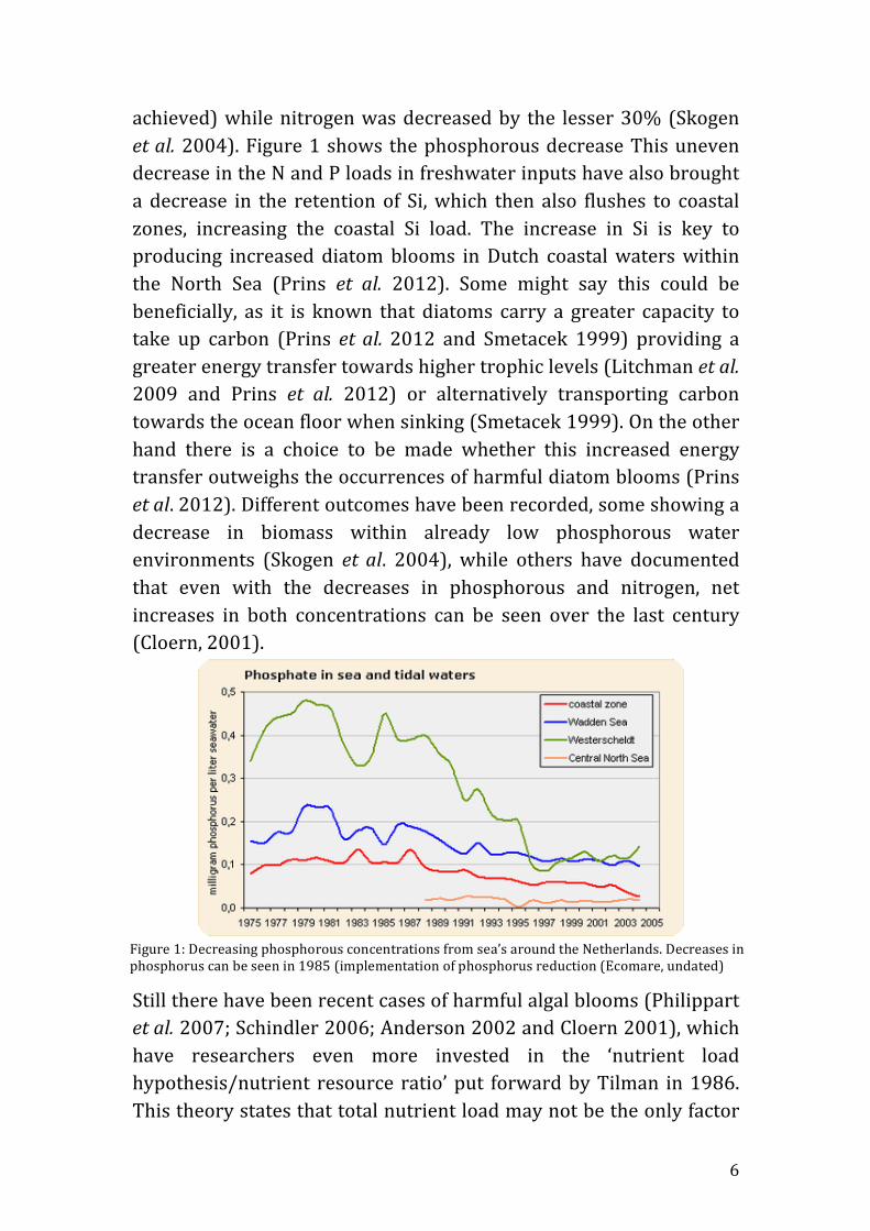
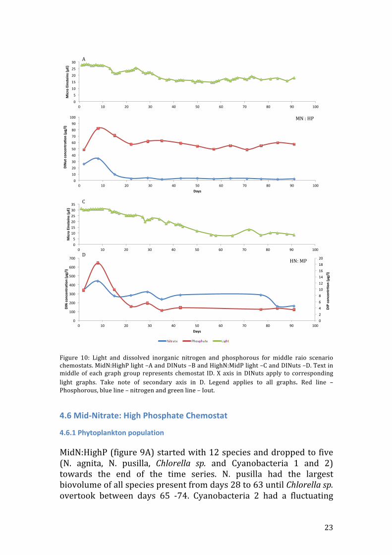
 Figure   8:   Light   and   dissolved   inorganic   nitrogen   and   phosphorous   for   extreme   limitation  scenario  chemostats  LowN:HighP  light  –A  and  DINuts  –B  and  HighN:LowP  light  –C  and  DINuts  –D.   Text   in   middle   of   each   graph   group   represents   chemostat   ID.   X   axis   in   DINuts   apply   to  corresponding   light  graphs.  Take  note  of  secondary  axis   in  D.  Legend  applies  to  all  graphs.  Red  line  –  Phosphorous,  blue  line  –  nitrogen  and  green  line  –  Iout.    

4.4  Low  Nitrate:  High  Phosphate  Chemostat  

4.4.1  Phytoplankton  population    Chemostat   LowN:HighP   (Figure   7A)   started   with   20   species   and  decreased   towards  11  by   the   start  of   the   third  week.  At   this   time  a  rapid  increase  in  biovolume  for  species  D.  minutissima,  N.  agnita,  N.  pusilla,  Chlorella  sp.  and  both  cyanbacteria  species  can  be  seen.  With  the   exclusion   of   D.   minutissima   these   five   species   constituted   the  

0"2"4"6"8"10"12"14"16"18"20"

0"

100"

200"

300"

400"

500"

600"

700"

0" 10" 20" 30" 40" 50" 60" 70" 80" 90" 100"DIP$concen

tra,

on$(μ

g/l)$

DIN$con

centra,o

n$(μg/l)$

Days$

0"

5"

10"

15"

20"

25"

30"

35"

0" 10" 20" 30" 40" 50" 60" 70" 80" 90" 100"

Micro&Einsteins&(μ

E)&

D  

C  

HN  :  LP  

0"

5"

10"

15"

20"

25"

30"

0" 10" 20" 30" 40" 50" 60" 70" 80" 90" 100"

Micro&Einsteins&(μ

E)&

0"

20"

40"

60"

80"

100"

120"

140"

160"

180"

0" 10" 20" 30" 40" 50" 60" 70" 80" 90" 100"

DINu

t.'concen

tra.o

n'(μg/l)'

Days'

B  

A  

LN  :  HP  

  21  

final  species  composition.  Species  D.  minutissima  increased  at  day  45  where  N.  pusilla,  Cyanobacteria  2  and  Chlorella  sp.  showed  opposite  trends.    

4.4.2  Abiotic  parameters    In   chemostat   LowN:HighP   (Figure   8A)   Iout   decrease   throughout  (26.8  to  23.9μE’s).  In  regards  to  nutrients  (Figure  8B)  DIP  remained  at  a  higher  concentration  then  DIN  from  the  second  week.  DIN  had  a  high  concentration  of  112.9μg/l  and  decreased  to  85.7μg/l  within  the  first   week.   It   remained   constant   until   the   fourth   week   where   DIN  decrease   suddenly   from   30.4   to   4.1μg/l   where   it   then   remained  under  10μg/l  with  the  exception  of  day  64  (tenth  week).  DIP  and  DIN  had  final  concentration  of  55.6  and  3.9μg/l,  respectively.    

4.5  High  Nitrate:  Low  Phosphate  Chemostat  

4.5.1  Phytoplankton  population    The   widest   range   of   species   were   present   at   the   start   (18)   of  HighN:LowP   (Figure   7B),   which   fell   to   five   towards   the   end   (N.  agnita,  N.  pusilla,  Chlorella  sp.  and  Cyanobacteria  1  and  2).  Cocconies  sp.   were   detected   during   days   53-­‐60   with   the   highest   overall  biovolume  at  day  60  of  3.53x108μm3/l  after  which  abundance  rapidly  dropped  to  below  detection.  Cyanobacteria  2  had  many  fluctuations  throughout  and  from  day  45  onwards  had  the  lowest  biovolume  of  all  five  species  until  day  70  where  an   increased  to  around  1x106μm3/l,  where  it  remained  constant  until  the  end.    

4.5.2  Abiotic  parameters    Chemostat   HighN:LowP   Iout   stayed   steady   until   day   23   where  numbers  fell  to  14μE’s  at  day  37  reaching  the  minimum  value  (figure  8C).   It   then   remained   constant  until   day  58  where   it   increased   and  leveled   out   at   around   22μE’s.   Looking   at   figure   8D,   DIN   remained  between   270.8   and   344.4μg/l   until   the   seventh   week   (day   35-­‐45)  where   the  concentration  rose   to  627.9  (DIN  maximum).  Two  weeks  after,   it   had   decreased   to   280μg/l   where   it   undulated   +/-­‐100μg/l  ending   on   a   concentration   of   605.2μg/l.   DIP   started   at   a  concentration   of   8μg/l   where   it   increased   to   12.4μg/l   by   day   15.  After   its   decrease   by   day   22   DIP   fluctuated   between   5.6   and   3μg/l  until  the  end  where  it  reached  a  final  concentration  of  2.5μg/l.      

  22  

           

   Figure   9:   Species   composition   in   boivolume   (μm3)   of   middle   ratio   scenario   chemostats.  MidN:HighP  (a)  and  HighN:MidP  (b).  Text  at  bottom  right  of  each  graph  refers  to  chemostat  ID.  Brown   lines   –   diatoms,   orange   line   –   dinoflagelatte,   green   line   –   Chlorella   sp.,   blue   lines–  cyanobacteria.  Dark  colours  represent  the  highest  biovolume  within  that  group.          

1"

10"

100"

1000"

10000"

100000"

1000000"

10000000"

100000000"

1E+09"

0" 10" 20" 30" 40" 50" 60" 70" 80" 90" 100"

Biovolum

e)(μm

3))

)

Days)

Skeletonema*costatum* Pseudonitzschia*delica3ssima* Cylindeotheca*closterium* Thallassiosira*angulata* Thallassiothrix*longissima* Navicula*directa*Pseudonitzschia*seriata* Coscinodiscus*sp.*(s)* Coscinodiscus*sp.*(l)* Tryblionella*sp.* Atheya*sp.* Bellerochea*malleus*Dinoflagellate*sp.* Thalassiosira*delicatula* Asterionellopsis*glacialis* Chaetoceros*affinis* Nitzschia)agnita) Pleurosigma*directa*Melosira*nummoloides* Nitschia)pusilla) Cocconies*sp.* Chlorella)sp.) Cyanobacteria)"1") Cyanobacteria)"2")

MidN  :  HighP  

A  

1"

10"

100"

1000"

10000"

100000"

1000000"

10000000"

100000000"

1E+09"

0" 10" 20" 30" 40" 50" 60" 70" 80" 90" 100"

Biovolum

e)(μm

3))

Days)Navicula(directa( Skeletonema(costatum( Cylindrotheca(closterium( Thallassiotrix(angulata( Dinoflagellate(sp.( Pseudonitzschia(seriata(Asterionellopsis(glacialis( Pseudonitzschia(delica@ssima( Atheya(sp.( Coscinodiscus(sp.((s)( Coscinodiscus(sp.((l)( Bellerochea(malleus(Cheatoceros(affinis( Dictyocha(sp.( Tryblionella(sp.( Chaetoceros(tor@ssimus( Nitzschia)agnita) Cocconies(sp.(Delphinies(minu@ssima( Navicula)pusilla) Chlorella)sp.) Cyanobacteria)"1") Cyanobacteria)"2")

B  

HighN  :  MidP  

  23  

 

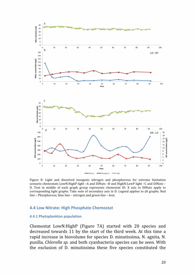
 Figure   10:   Light   and   dissolved   inorganic   nitrogen   and   phosphorous   for   middle   raio   scenario  chemostats.  MidN:HighP  light  –A  and  DINuts  –B  and  HighN:MidP  light  –C  and  DINuts  –D.  Text  in  middle   of   each   graph   group   represents   chemostat   ID.   X   axis   in  DINuts   apply   to   corresponding  light   graphs.   Take   note   of   secondary   axis   in   D.   Legend   applies   to   all   graphs.   Red   line   –  Phosphorous,  blue  line  –  nitrogen  and  green  line  –  Iout.    

4.6  Mid-­‐Nitrate:  High  Phosphate  Chemostat  

4.6.1  Phytoplankton  population    MidN:HighP  (figure  9A)  started  with  12  species  and  dropped  to  five  (N.   agnita,   N.   pusilla,   Chlorella   sp.   and   Cyanobacteria   1   and   2)  towards   the   end   of   the   time   series.   N.   pusilla   had   the   largest  biovolume  of  all  species  present  from  days  28  to  63  until  Chlorella  sp.  overtook   between   days   65   -­‐74.   Cyanobacteria   2   had   a   fluctuating  

0"

10"

20"

30"

40"

50"

60"

70"

80"

90"

100"

0" 10" 20" 30" 40" 50" 60" 70" 80" 90" 100"

DINut&con

centra-o

n&(μg/l)&

Days&

0"

5"

10"

15"

20"

25"

30"

0" 10" 20" 30" 40" 50" 60" 70" 80" 90" 100"

Micro&Einsteins&(μ

E)&

A  

MN  :  HP  

0"5"10"15"20"25"30"35"

0" 10" 20" 30" 40" 50" 60" 70" 80" 90" 100"

Micro&Einsteins&(μ

E)&

0"2"4"6"8"10"12"14"16"18"20"

0"

100"

200"

300"

400"

500"

600"

700"

0" 10" 20" 30" 40" 50" 60" 70" 80" 90" 100"DIP$concen

tr+o

n$(μg/l)$

DIN$con

centra+o

n$(μg/l)$

Days$

D  

C  

HN:  MP  

  24  

biovolume  throughout,  and  at  day  18  became  one  of  the  lowest  three  biovolumes.   It   then   drastically   increased   from   4114μm3/l   to  1x108μm3/l   outcompeting   all   species   for   the   largest   biovolume   for  the  last  two  days.  

4.6.2  Abiotic  factors    In  MidN:HighP   Iout     started   at   27.9μE’s   and   remained   steady   until  day   10  where   it   decreased   and   reached   21.4μE’s   by   day   16   (figure  10A).   It   then   proceeded   to   increase   again   to   25.5μE’s   by   day   24   to  which   it  decreased  steadily   to  day  56  (14.6μE’s).  From  here  on  Iout  fluctuated   until   the   end   ranging   between   14.6   and   18.1μE’s.   From  weeks  one  to  two  (days  2  to  8)  both  DIN  and  DIP  increased,  DIN  from  26.1  to  34.7μg/l  and  DIP  from  48.9  to  almost  double  at  82.5μg/l.  DIN  and  DIP  stayed  at  a  constant  level  further  on  the  time  series  (with  a  slight   fluctuation   in  DIP  during  day  60-­‐91)  ending  on  concentration  of  2.3  and  57.4μg/l  respectively  (Figure  10B).      

4.7  High  Nitrate:  Mid-­‐Phosphate  chemostat  

4.7.1  Phytoplankton  population    In   the   HighN:MidP   (figure   9B)   nine   species   were   recorded   at   day  three  which   increased   to  16  by  day  nine   to  which   species  diversity  declined  until  5   species   left   (day  30)   (N.   agnita,  N.  pusilla,  Chlorella  sp.   and   Cyanobacteria   1   and   2),   with   the   exception   of   Cocconies   sp  appearing  at  day  58.  Chlorella  sp.  dominated   in  biovolume  from  day  42   until   the   end   with   Cyanobacteria   1   and   N.   agnita   switching  between   second   and   third.   Cyanobacteria   2   had   the   lowest  biovolume.    

4.7.2  Abiotic  parameters    The   HighN:MidP   chemostat   (figure   10C)   showed   a   steady   decrease  throughout   with   the   exception   of   day   71   where   the   alternative  chemostat  was  measured   (due   to  breakage).  Overall   Iout  decreased  from   a   value   of   31.4μE’s   to   8.5μE’s.   Both   DIN   and   DIP   showed   a  similar  trend  throughout  (figure  10D).  DIN  started  at  a  concentration  of  341μg/l  and  increased  to  442.5  in  the  first  week  then  decreased  to  277.2μg/l   where   it   stayed   constant   throughout   and   decreased   to  158.8μg/l   in   the   last   2   weeks.   DIP   started   at   9.6μg/l   where   it  increased  2-­‐fold  in  the  first  week  (18.4μg/l).  During  the  third  week  it  decreased  to  4.5μg/l  and  remained  constant  between  5.5  and  3μg/l.    

  25  

 Figure  11:  Comparing  diversity  (A)  and  dominance  (B)  between  chemostats  at  day  one.  Diversity  calculated  by  quarter  root  of  day  one  counts.  

Table   2:   Sorensen   index   comparing   similarity   (presence   or   absence   of   species)   of   the   start  composition   between   each   chemostat   (equation   in   method   section).   A   Sorensen   index   of   1  indicates  100%  similarity,  0  means  100%  dissimilar    

4.9  All  chemostats:  Summary  

4.9.1  Beginning    The   beginning   composition   of   all   chemostats   was   varied.   The  extreme   conditions   and   low   load   (LowN:HighP,   HighN:LowP   and  LowN:LowP)   contained   the   largest   diversity   with   18,   17   and   14  species   respectively   (Figure   11A).   The   remaining   chemostats  contained   eight   species   while   MidN:HighP   contained   nine.   The  chemostats   LowN:LowP,   MidN:HighP   and   MidN:MidP   showed   a  dominance   by   Chlorella   sp.   (Figure   11B).   In   HighN:HighP  Thallasiothrix  angulata  seems  to  be  the  most  dominant  at  70%.    The  

!! LH! LL! HH! HM! HL! MH! MM!LH! !! 0.81! 0.62! 0.64! 0.80! 0.52! 0.54!LL! 0.81! !! 0.64! 0.55! 0.77! 0.52! 0.64!HH! 0.62! 0.64! !! 0.38! 0.56! 0.71! 0.50!HM! 0.64! 0.55! 0.38! !! 0.56! 0.47! 0.75!HL! 0.80! 0.77! 0.56! 0.56! !! 0.54! 0.56!MH! 0.52! 0.52! 0.71! 0.47! 0.54! !! 0.71!MM! 0.54! 0.64! 0.50! 0.75! 0.56! 0.71! !!!

  26  

Sorensen  index  in  table  2  shows  that  all  chemostats  were  dissimilar  at  the  onset.  The  most  similar  was  LowN:HighP  and  LowN:LowP  with  81%   similarity   in   species.   MidN:HighP   and   HighN:MidP   were   the  least   similar  with  a   score  of  47%  similarity.  All   chemostats   showed  low  species  population  with  high  species  diversity.  

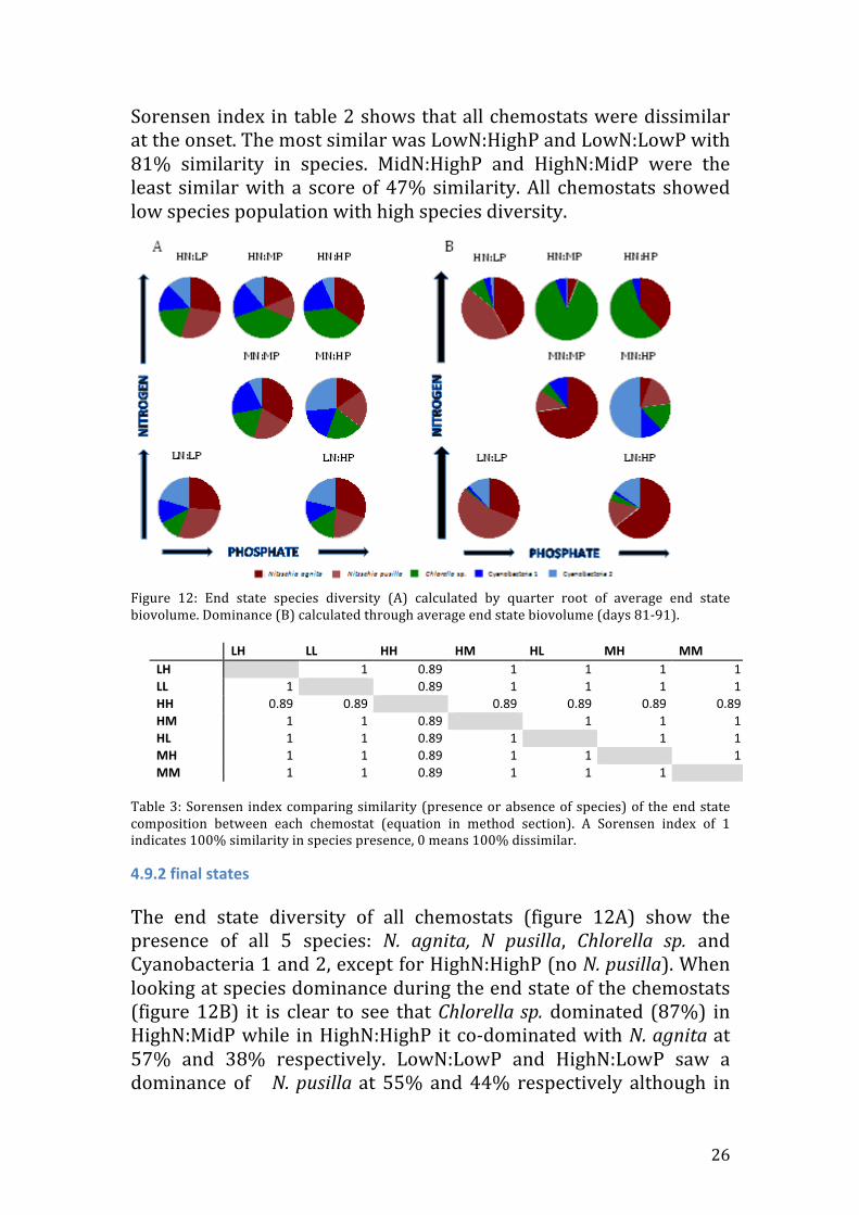
 Figure   12:   End   state   species   diversity   (A)   calculated   by   quarter   root   of   average   end   state  biovolume.  Dominance  (B)  calculated  through  average  end  state  biovolume  (days  81-­‐91).    

Table  3:  Sorensen   index  comparing  similarity  (presence  or  absence  of  species)  of   the  end  state  composition   between   each   chemostat   (equation   in   method   section).   A   Sorensen   index   of   1  indicates  100%  similarity  in  species  presence,  0  means  100%  dissimilar.  

4.9.2  final  states    The   end   state   diversity   of   all   chemostats   (figure   12A)   show   the  presence   of   all   5   species:   N.   agnita,   N   pusilla,   Chlorella   sp.   and  Cyanobacteria  1  and  2,  except  for  HighN:HighP  (no  N.  pusilla).  When  looking  at  species  dominance  during  the  end  state  of  the  chemostats  (figure  12B)   it   is   clear   to   see   that  Chlorella  sp.   dominated   (87%)   in  HighN:MidP  while   in  HighN:HighP   it  co-­‐dominated  with  N.  agnita  at  57%   and   38%   respectively.   LowN:LowP   and   HighN:LowP   saw   a  dominance   of      N.  pusilla  at   55%  and  44%   respectively   although   in  

!! LH# LL# HH# HM# HL# MH# MM#LH# !! 1! 0.89! 1! 1! 1! 1!LL# 1! !! 0.89! 1! 1! 1! 1!HH# 0.89! 0.89! !! 0.89! 0.89! 0.89! 0.89!HM# 1! 1! 0.89! !! 1! 1! 1!HL# 1! 1! 0.89! 1! !! 1! 1!MH# 1! 1! 0.89! 1! 1! !! 1!MM# 1! 1! 0.89! 1! 1! 1! !!!

  27  

the   HighN:LowP   N.   agnita   co-­‐dominated   contributing   42%   of   the  total  biomass.   In   the  cases  of  MidN:MidP  and  LowN:HighP  N.  agnita  dominated   in   both   cases   with   73%   and   65%   respectively.  Cyanobacteria   2   dominated   50%   of   the   species   biovolume   in  MidN:HighP.  The  Sorensen  index  in  table  3  shows  that  all  chemostats  are   100%   similar   (values   of   1)   while   that   of   the   HighN:HighP   was  different  from  the  rest  with  89%  similarity.  

                                 

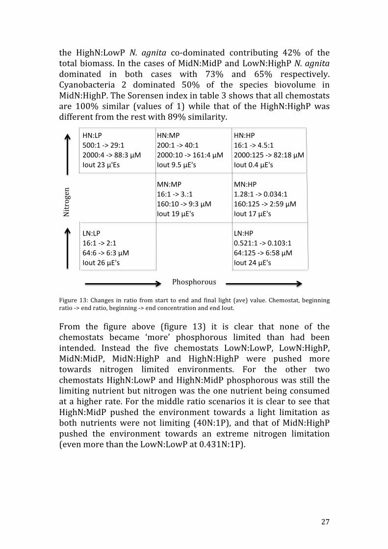
   Figure  13:  Changes   in   ratio   from   start   to   end   and   final   light   (ave)   value.   Chemostat,   beginning  ratio  -­‐>  end  ratio,  beginning  -­‐>  end  concentration  and  end  Iout.    From   the   figure   above   (figure   13)   it   is   clear   that   none   of   the  chemostats   became   ‘more’   phosphorous   limited   than   had   been  intended.   Instead   the   five   chemostats   LowN:LowP,   LowN:HighP,  MidN:MidP,   MidN:HighP   and   HighN:HighP   were   pushed   more  towards   nitrogen   limited   environments.   For   the   other   two  chemostats  HighN:LowP  and  HighN:MidP  phosphorous  was   still   the  limiting  nutrient  but  nitrogen  was  the  one  nutrient  being  consumed  at  a  higher  rate.  For  the  middle  ratio  scenarios  it   is  clear  to  see  that  HighN:MidP   pushed   the   environment   towards   a   light   limitation   as  both   nutrients  were   not   limiting   (40N:1P),   and   that   of  MidN:HighP  pushed   the   environment   towards   an   extreme   nitrogen   limitation  (even  more  than  the  LowN:LowP  at  0.431N:1P).      

Phosphorous  

Nitrogen  

HN:LP HN:MP HN:HP500:1*+>*29:1 200:1*+>*40:1 16:1*+>*4.5:12000:4*+>*88:3*μM 2000:10*+>*161:4*μM 2000:125*+>*82:18*μMIout*23*μ'Es Iout*9.5*μE's Iout*0.4*μE's

MN:MP MN:HP16:1*+>*3.:1 1.28:1*+>*0.034:1160:10*+>*9:3*μM 160:125*+>*2:59*μMIout*19*μE's Iout*17*μE's

LN:LP LN:HP16:1*+>*2:1 0.521:1*+>*0.103:164:6*+>*6:3*μM 64:125*+>*6:58*μMIout*26*μE's Iout*24*μE's

  28  

V.  Discussion      Looking   at   both   the   biovolume   and   dissolved   nutrient/light   graphs  correlations  between  the  two  can  be  seen.  The  beginning  of  all  seven  chemostats  shows  a  high  diversity  but  relatively  low  biovolume.  Due  to  the  low  abundance  (low  biovolume)  but  relatively  high  diversity  of  species,   the   flow-­‐through   rate   of   nutrients   was   quicker   than   the  consumption   rates,   especially   by   small,   low   storage   capacity   cells  such   as   Chlorella   sp.   and   cyanobacteria   2.   After   a   couple   of   weeks  competition  was   strong  which   can   be   seen   by   the   species   diversity  decreased   and   the   subsequent   shifted   in   composition   towards   one  dominated   with   diatoms   and   dinoflagellates   such   as   in   the   case   of  LowN:LowP.   This   increase   in   size   (diatoms/dinoflagellates)   and  abundance   cause   nutrient   consumption   to   increase,   which   is  reflected  in  the  prominent  decreases  (around  day  20)  in  all  DIN  and  DIP   graphs   except   HighN:HighP   due   to   its   extremely   high   load  meeting  no  match  of  consumption  until  around  day  50.    

5.1  Species  and  their  limiting  nutrients    When   looking   at   species   and   their   effect   on   nutrients   (DIN/DIN)  more   correlations   can  be   found.   For   example   in   LowN:LowP  where  the  slight  increase  in  DIP  during  days  43-­‐49  show  a  correlation  with  species  N.  pusilla,  Triblionella  sp.  and  Cocconies  sp.  When  comparing  graphs  (5A  and  8A)  at  day  49  N.  pusilla  biovolume  decreased  where  DIP   increased.  This  could  be  due   to  N.  pusilla  previously  consuming  more  phosphorous  than  other  species  present,  thus  when  biovolume  (abundance)   decreases   the   phosphorous   within   the   chemostat  increases.  Triblionella  sp.  was  not  recorded  after  day  44,  which,  if  like  N.  pusilla,  also  had  a  high  affinity  for  phosphorous  could  contribute  to  the   increase   in   phosphorous   availability.   At   day   77,   N.   agnita  decreased   while   all   other   four   species   increased   causing   a   slight  increase  in  the  DIP  availability  within  the  system.  This  gives  evidence  of   a   low  R*  value   for  diatoms   in   regards   to  phosphorous   leading   to  diatoms   being   the   best   competitors   for   phosphorous   which  corresponds   to   previous   research   (Tilman   et   al.,  1986)  where   they  

  29  

too   found   diatoms   to   be   superior   competitors   in   phosphorous  limitation   which   may   be   due   to   the   eradication   of   predation   from  dinoflagellates  (Hu  et  al.,  2011).    HighN:HighP,  due  to  the  extreme  high  load  of  nutrient  input,  showed  no   change   in   DIN   or   DIP  when   the   biovolume   increased,   even   at   a  biovolume  of  approximately  1.0  X  107  which  can  be  seen  by  the  large  decrease   in   light   (high   abundance   of   species)   in   figures   4C,   8E   and  8F).  During  days  50-­‐72   a   large  decrease   in  DIN  occurred   (142μg/l)  which   coincided   with   Chlorella   sp.   and   cyanobacteria   2   increase,  giving   evidence   to   the   notion   that   both   species   are   nitrogen  competitors   (Wang   et  al.,   2013).   This  may   also   be   due   to   the   small  size   cyanobacteria   and  Chlorella   sp.   share,   compared   to   diatoms,   as  these  tend  to  require  more  nitrogen  than  phosphorous  (Maranon  et  al.,  2013)   therefore   through  the   increased  consumption  of  nitrogen,  reduced  the  nitrogen  within  the  chemostat.      Within   all   three   load   scenarios,   the   onset   of   final   state   species  diversity   appeared   earlier   as   load   increased.   In   HighN:HighP   the  onset  appeared  at  day  29,  MidN:MidP  on  day  35  and  in  LowN:LowP  on   day   43.   This   shows   that   increased   load   invoke   a   more   intense  competition   therefore   producing   dominance   earlier.   Tubay   et   al.,  (2013)  reported  that  low  levels  of  nutrients  produce  a  lower  level  of  competition.   This   coheres  with   other   studies   that   have   shown   that  eutrophication   (increase   in   nutrient   load)   can   lead   to   an   increased  biomass   of   phytoplankton   (blooms)   which   lead   to   diversity   loss  (Tubay  et  al.,  2013  and  Anderson  et  al.,  2002).  These  blooms  can  be  toxic/harmful   although   not   all   HABs   are   linked   with   nutrient  enrichment  (Anderson  et  al.,  2002).  

5.1.1  ‘pushing’  nutrient  environments    When  looking  at  how  the  species  composition  push  the  environments  in   MidN:HighP   and   HighN:MidP,   figure   13   showed   that   limitations  were   pushed   to   extremes.   MidN:HighP   was   pushed   towards   an  extreme   nitrogen   limitation   (0.034:1)   even   more   extreme   than  LowN:HighP  (0.103:1).  Similarly  HighN:MidP  was  pushed  towards  a  light   limitation,  as  both  nutrients  were  not   limiting  enough  to  cause  

  30  

nutrient  limitation.    HighN:HighP  although  having  a  lower  Iout  value  then  HighN:MidP  also  produced  an  end  ratio  of  4.5N:1P  showing  the  chemostat   to   be   co-­‐limited   (Nitrogen   and   light).   This   particularly  shows   that   species   composition   is   important   as   the   species   most  competitive   will   reduce   their   limiting   resources   to   their   lowest   R*  (Tilman,   1982)   present   in   the   environment   as   said   in   the  introduction,   therefor   unavailable   to   other   species   (Litchman   et  al.,  2012).   In   the   cases  of   the  other   five   chemostats,   all   appeared   to  be  ‘more’  nitrogen  limited  then  phosphorous  limited  which  correlates  to  Anderson  et  al.,  2002  which  showed  a   relationship  between  marine  phytoplankton   production   and   nitrogen.   HighN:LowP   and  HighN:MidP   were   the   only   two   chemostats   to   show   signs   of  phosphorous   limitation   (29N:1P   and   40N:1P   respectively).   This   fits  previous   consensus   showing   nitrogen   to   be   the   limiting   nutrient  (Howarth  and  Marino,  2006).    

5.2  Species  dominance  (beginning  and  end  state)  To  understand  why  certain  species  dominated  or  why  environments  were   pushed   figure   11B,   12B   and   13   must   be   taken   into  consideration.  N.  pusilla   clearly   is   favorable   towards   low  phosphate  environment   which   would   grant  N.   pusilla   the   lowest   R*   value   for  phosphorous  therefore  outcompeting    all  other  species  (competitive  exclusion)  (Tilman  et  al.,  1986).  In  HighN:LowP  however  N.  agnita  is  co-­‐dominating  proposing  that  is  has  broader  N:P  tolerance  rage.  Due  to  both  having  similar  biovolume  it  can  be  assume  N.  agnita  has  the  lowest   R*   for   nitrogen   therefor   both   species   are   able   to   co-­‐exist  together  (trade  offs).  To  further  the  statement  that  N.  agnita  has  the  lowest  R*  for  nitrogen  we  can  look  at  HighN:MidP  and  HighN:HighP.  Here  the  light  limitation  predicted  turned  out  to  be  a  co-­‐limitation  of  nitrogen   and   light   while   chemostat   HighN:MidP   was   clearly   light  limiting   as   both   nutrients   were   not   limiting.   The   N:P   ratio   shifted  towards   N   limitation   rather   than   exasperating   P   limitation,   which  would   have   been   the   predicted   nutrient   to   become   limiting.   If  Chlorella  sp.  was  dominant   in   low   light   conditions   it  must   have   the  lowest  R*   for   light  resources.  This   implies  successful  competition   in  

  31  

HighN:HighP  for  the   light  which  fits   theory  that  Chlorella  sp.  are  the  best  competitors  for  light  (Tilman  et  al.,  1986).      Stole  et  al.,  (1994)  stated  that  in  eutrophic  conditions  phytoplankton  of   larger   sizes   would   dominate   due   to   their   increased   storage  availability,   but   when   compared   to   the   light   limiting   –   eutrophic  (HighN:MidP)  conditions  it  is  clear  that  Chlorella  sp.  dominated  even  though  much  smaller  than  all  diatoms.  While  N.  agnita  is  not  present  in   low   light   conditions   (HighN:MidP)   it   is   present   in   low   light   and  nitrogen   limited   conditions   (HighN:HighP).  This   gives  evidence   that  N.  agnita  may  be  the  source  of  the  nitrogen  limitation  in  HighN:HighP  due  to  its  high  affinity  for  nitrogen.  This  also  connects  to  MidN:MidP  and   LowN:HighP    where  N.  agnita   is   a   stronger   competitor   (strong  grower)  in  condition  that  are  initially  16N:1P,  but  is  able  to  skew  the  availability   of   nutrient   towards   N   limitation   and   still   thrive,   thus  outgrowing  its  competitors.      

       

   However   in   extremely   low   nitrate   conditions   cyanobacteria   2  were  able   to   survive   (LowN:LowP   and   LowN:HighP).   Although   not  dominating   like   N.   pusilla   or   N.   agnita   most   likely   due   to   species  biovolume   (Maranon  et  al.,   2013   and   Irwin  et  al.,   2006)   as  diatoms  are  larger  and  therefore  able  to  take  up  more  nutrients  than  required  (as   well   as   have   a   larger   storage   capacity)   than   smaller  phytoplankton.  As  a  trade-­‐off  larger  phytoplankton  growth  is  limited  by   biomass.     When   nitrogen   limitation   is   extreme   (MidN:HighP   -­‐  

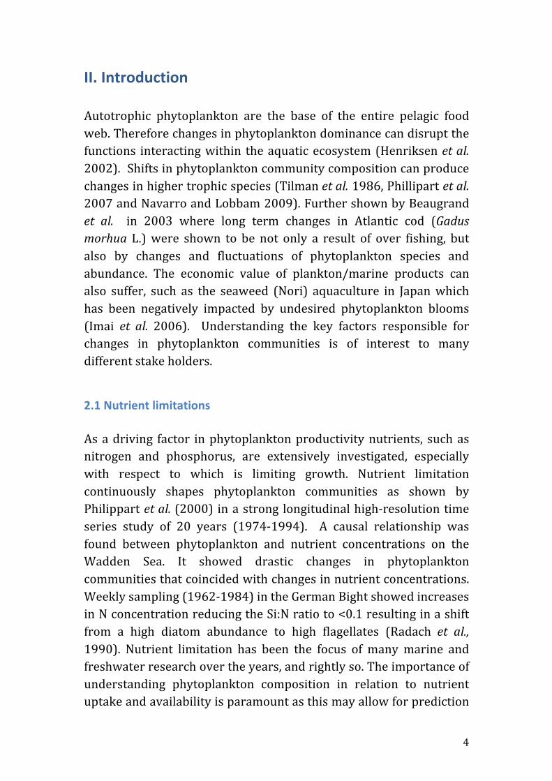
Figure  14:  Pictures  of  final  state  species  A)  Cyanobacteria  1,  B)  Cyanobacteria  2,  C)  Chlorella  sp.,  D)  Nitzschia  pusilla,  E)  Nitzschia  agnita.  All  photos  at  50X  using  water  immersion  lense.  Scale  bar  in  E  applies  to  all.  

A   B   C  

D   E  

  32  

0.034N:1P)   the   diatom’s   need   for   nitrogen   isn’t   met   therefore  allowing  cyanobacteria  2  to  over-­‐take  and  out  compete.      In   low   nutrient   oceanic  waters  mutualistic   relationships   have   been  found  between  diatoms   and  nitrogen   fixing  bacteria   (heterocystous  cyanobacteria)  where  heterocystous  cyanobacteria  provide  nitrogen  to   the  diatoms   in   close  proximity   sometimes  even  30  minutes   after  fixation   (Foster   et   al.     2011).   In   some   cases   as   with   Richelia   and  Calothrix   (heterocystic   cyanobacteria)   an   overload   of   nitrogen  fixation   was   encountered   and   more   than   90%   of   the   total   fixed  nitrogen  is  transferred  to  the  diatom  partner.      After  biochemical  analysis  performed  by  a  colleague  on  the  CHARLET  cruise  (Julia  Grosse)  the  low  nitrogen  chemostats  showed  evidence  of  nitrogen   fixation.   This   suggests   that   cyanobacteria   2   is   a   nitrogen  fixating   cyanobacteria   capable   of   withstanding   low   nitrogen  environments,  which  explains  the  51%  dominance  of  cyanobacteria  2  within   the   MidN:HighP   chemostat.   This   finding   also   coincides   with  Michard   et   al.   (1996)   where   he   too   concluded   through   water  observations   of   the   French   reservoir   that   cyanobacteria   blooms   (in  this  case  Microcystis  aeruginosa)  were  forming  when  the  ratio  of  N:P  was  less  than  5  (such  as  our  MidN:HighP)  therefore  concluding  that  cyanobacteria   would   dominant   in   low   nitrogen   environments.   This  study   however   looked   at   a   reservoir   where   water   stratification  would  be   imminent  due   to   low  or  no   turbulence  making  conditions  perfect   for   cyanobacteria   to   float   to   the   top   of   the   water   column  through   gaseous   vesicles   within   their   cells   (Huisman   et   al.,   2004).  Using   Huiman   et   al   2004   findings   of   low   turbulence   favoring  cyanobacteria   and   turbulent   environments   favoring   diatoms   and  Chlorella  sp.,   perhaps   if   this   study  was   repeated  with  no   turbulence  (air   mixing)   a   different   composition   would   arise   favoring  cyanobacteria.        

  33  

5.3  Summary  of  end  state  species    In  summary  it  can  be  said  that  N.  pusilla  is  the  best  competitor  in  low  phosphorous   conditions,   Chlorella   sp.   for   low   light   conditions,   N.  agnita  and  cyanobacteria  2  for  low  and  very  low  nitrogen  conditions,  respectively   and   cyanobacteria   1   is   able   to   withstand   exclusion.  Overall  diatoms  are  better  competitors  in  low  nutrient  loads  and  low  phosphorous  environments  while  Chlorella  sp.  thrive  in  high  nutrient  and  low  light  conditions  (Potapova  and  Charles  2002;  Kilham  1986)  while  nitrogen  fixing  cyanobacteria  are  superior  in  extreme  nitrogen  limitations  (Vrede  et  al.,  2009;  Ekhom,  2008  and  Tilman  et  al.,  1986).        Species   diversity   may   shift   (through   competition)   by   changing  nutrient   ratios   in   low   nutrient   conditions   (Anderson   et   al.,   2002).  Nutrient  ratio  (N:P)  can  also  be  a  good  predictor  for  the  presence  of  nitrogen  fixing  cyanobacteria  in  ratio’s  less  than  16N:1P  (Vrede  et  al.,  2009).  On  the  other  hand  nutrient  load  (LowN:LowP,  MidN:MidP  and  HighN:MidP)   becomes   a   better   predictor   for   species   dominance  especially   in   high   nutrient   conditions   producing   a   stronger  competition  (resulting  diversity  loss).      From   the   results   we   can   say   that   the   North   Sea   shows   signs   of  nitrogen  limitation  due  to  the  increased  nitrogen  consumption  in  all  chemostats.  Both  ratio  and   load  are   important   in  predicting  species  composition   where   load   is   more   important   in   light   limiting  conditions  and  in  phytoplankton  dominance.  If  nutrient  ratio  and  or  load   change   in   controlled   environments   then   phytoplankton  composition   changes.   The   change,   as   to   whether   the   composition  diversity  or  dominance  will  change  all  depends  on  what  the  nutrient  change  will   alter,   ratio   or   load.   For   the  North   Sea   this   still   remains  uncertain   due   to   its   dynamic   system   but   perhaps   small   changes   in  either  direction   (dominance  or  diversity)  may  appear  with  nutrient  changes   in   the   North   Sea.     From   the   study   one   could   accept   an  increased  load  (during  pre-­‐spring  bloom)  to  increase  the  likely  hood  of  green  algae  blooms.      

  34  

Care  must  be   taken  when  dealing  with  management  of  nutrients  as  nitrogen   and   phosphorous   are   linked  meaning   that   changes   in   one  may   effect   the   other   such   as   in   the   Baltic   Sea   where   depletions   of  nitrogen   could   stimulate   nitrogen   fixing   cyanobacteria   causing   an  increased   risk  of   blooms   (Ekholm  2008).  Alternatively   this   reduced  nitrogen   load   could   decrease   phytoplankton   biomass   therefore  contributing   towards   the   release   of   phosphorous   from   sediments  therefore   lowering   the   chance   of   cyanobacteria   blooms   (Ekholm,  2008)  therefore  shifting  toward  diatom  dominated  waters.  

5.3  Limitations    With   controlled   environments   however   come   disadvantages   when  applying  to  the  field,  as  stable  states  are  rare  to  come  across  due  to  intermittent   nutrient   fluxes   favoring   larger   diatoms   than   constant  supply   (Litchman   et   al.   2009)   and   constant   changing   physical  environments   such   as   temperature   dependence   which   has   been  shown   to  have   an   effect   on   species  dominance   (Tilman  et  al  1986).  Perhaps   the   temperature   of   the   chemostats   during   this   experiment  altered   the   original   composition   as   different   seasons   would  (Anderson   et   al.,   2002   and   Potapova   2002).   Predation   is   also   an  important   factor   where   in   this   experiment   dinoflagellates   were  eliminated   by   week   two   allowing   other   species   to   compete   where  otherwise  not  (Anderson  et  al.,  2002  and  Elser  et  al.  1988).  Research  conducted   on   the   role   of   grazers   (zooplankton)   also   showed  interesting   findings.   It   has   been   suggested   that   grazers   alter   the  nutrient  limitation  patters  and  therefore  communities  receiving  their  nutrients   through   grazers   are   either   to   become   nitrogen   or  phosphorous  limited  but  not  both  (Sterner  1990).  The  study  used  pre  spring  bloom   inoculum  where  abundance  was  very   low  at   the   start  giving  no  prior  nutrient  limitation  or  adaptive  species  a  head  start.      In   the   future   comparing  mid/post   spring   bloom   inoculum  with   the  results   of   the   present   study   would   prove   beneficial.   Would   the  diversity  of  mid/post  end  states  prove  a  similar  diversity  (in  respect  to  number  and  similarity  of  diversity)  and  would   they  show  similar  dominance  in  regards  to  species?  

  35  

 

5.4  conclusion      To  answer  the  questions  of  this  paper  ‘will  changes  in  N:P  ratio  impact  the  phytoplankton  community  of  the  North  Sea?’  from  the  results  it  can  be  said  that  changes  in  nutrient  ratio  and  load  have  the  potential  to  change  phytoplankton  composition.  The  maximum  degree  to  which  these  change  in  composition  can  be  predicted  only  lies  within  the  different  groups  of  phytoplankton  (diatom,  dinoflagellate,  green  algae,  cyanobacteria  etc.).    

VI.  Reference  list    Anderson  D.  M,  Glibert  P.  M  ad  Burkholder  J.  M  (2002)  ‘Harmful  alfal  blooms  and  eutrophication:  nutrient  sources,  composition,  and  consequences’  Estuaties.  25  (4b)  :  704-­‐726    Beaugrand  G,  Brander  K.M,  Lindley  J.  A,  Souissi  S  and  Reid  P.  C  (2003)  ‘Plankton  effect  on  cod  recruitment  in  the  North  Sea’  Nature.  426  :  661-­‐664    Brauer  V.  S,  Stomp  M,  Huisman  J  (2012)  ‘The  nutrient-­‐load  hypothesis:  Patterns  of  resource  limitation  and  community  structure  driven  by  competition  for  nutrients  and  light’  The  American  naturalist.  127  (6)  :  179-­‐740      Bulgakov  N.  G  and  Levich  A.  (undated)  ‘The  nitrogen:phosphorus  ratio  as  a  factor  regulating  phytoplankton  community  structure’  [online]  http://www.chronos.msu.ru/EREPORTS/levich_the_nitrogen/levich_the_nitrogen.htm    Cadee  G.  C  (1986)  ‘Recurrent  and  changing  seasonal  patterns  in  phytoplankton  of  the  westernmost  inlet  of  the  Dutch  Wadden  Sea  from  1969  to  1985’  Marine  biology.  93  :  281-­‐289    

  36  

Cloern  J.  E  (2001)  ‘Our  evolving  conceptual  model  of  the  coastal  eutrophication  problem’  Marine  ecology  progress  series.  210  :  223-­‐253    Dow  A.  R,  Gilliand  J.  L,  Raymond  R.  A  and  Shiring  J.  J  (2006)  ‘Competition  between  Chlorella  sp.  and  Chlorococcum  sp.:  a  study  in  nutrient  limitation’  Journal  of  ecological  research.  8  :  20-­‐25    Downing  J.  A,  Watson  S.  B  and  McCauley  E  (2001)  ‘Predicting  cyanobacteria  dominance  in  lakes’  Candaian  journal  of  fisheries  and  aquatic  sciences.  58  (10)  :  1905-­‐1908    Ecomare  (undated)  http://www.ecomare.nl/en/encyclopedia/natural-­‐environment/matter-­‐and-­‐materials/nutrients/phosphoric-­‐compounds/  [accessed  on  3/3/2014]    Ekholm  (2008)  [online]  http://www.cost869.alterra.nl/FS/FS_NPratio.pdf  [accessed  on  19/12/2013]    Elser  J.  J,  Bracken  M.  E.  S,  Cleland  E.  E,  Gruner  D.  S,  Harpole  W.  S,  Hillebrand  H,  Ngai  J.  T,  Seabloom  E.  W,  Shurin  J.  B  and  Smith  J.  E  (2007)  ‘Global  analysis  of  nitrogen  and  phosphorous  limitation  of  primary  producers  in  freshwater,  marine  and  terrestrial  ecostystems’  Ecology  letters.    10  :  1135-­‐1142    Elser  J.  J,  Elser  M.  M,  sMackay  N  and  Carpenter  S.  R  (1988)  ‘Zooplankton-­‐mediated  transitions  between  N-­‐  and  P-­‐limited  algal  growth’  Limnology  and  oceanography.    33  (1)  :  1-­‐14    Fisher  T.  R,  Carlson  P.  R  and  Barber  R.  T  (1982)  ‘Carbon  and  nitrogen  primary  productivity  in  three  North  Carolina  estuaries’  Estuarine,  coastal  and  shelf  science.  15  (6)  :  621-­‐644    Foster  R.  A,  Kuypers  M.  M.  M,  Vagner  T,  Paerl  R.  W,  Musat  N  and  Zehr  J.  P  (2011)  ‘Nitrogen  fixation  and  transfer  I  nopen  ocean  diatom-­‐cyanobacterial  symbioses’  Multidisciplinary  journal  of  microbial  ecology.  5  (9)  :  1484-­‐1493    

  37  

Fukuyo  Y,  Imai  I,  Kodama  M  and  Tamai  K  (undated)  [online]  http://www.pices.int/publications/scientific_reports/report23/HAB_Japan.pdf    Groove  J.  P  (2000)  ‘Resource  competition  and  community  structure  in  aquatic  micro-­‐organisms:  experimental  studies  of  algae  and  bacteria  along  a  gradient  of  organic  carbon  to  inorganic  phosphorous  supply’  Journal  of  plankton  research.  22  98)  :  1591-­‐1610    Graneli  E  and  Sundback  K  (1985)  ‘The  response  of  planktonic  and  microbenthi  algal  assemblages  to  nutrient  enrichment  in  shallow  coastal  waters,  southwest  Sweden’  Journal  of  experimental  marine  biology  and  ecology.  85  (3)  :  253-­‐268    Hecky  R.  E  and  Kilham  P  (1988)  ‘Nutrient  limitation  on  phytoplankton  freshwater  and  marine  environments:  a  review  of  recent  evidence  on  the  effects  of  enrichment’  Limnology  and  oceangrapthy.  33  :  786-­‐822    Henriksen  P,  Riemann  B,  Kaas  H,  Sorensen  H.  M  and  Sorensen  H.  L  (2002)  ‘Effects  of  nutreitn-­‐limitation  and  irradiance  on  marine  phytoplankton  pigments’  Journal  of  plankton  research.  24  (9)  :  835-­‐858    Howarth  R.  W  and  Marino  R  (2006)  ‘Nitrogen  as  the  limiting  nutrient  for  eutrophication  in  coastal  marine  ecosystems:  evolving  views  over  three  decades’  Limnology  and  oceanography.    51  (1  pt.2)  :  364-­‐376    Hu  H,  Zhang  J  and  Chen  W  (2011)  ‘Competition  of  bloom-­‐forming  marine  phytoplankton  at  low  nutrient  concentrations’  Journal  of  environmental  science.  23  (4)  :  656-­‐663    Huisman  J,  Sharples  J,  Stroom  J.  M,  Visser  P.  M,  Kardinaal  W.  E.  A,  Verspagen  J.  M.  H  and  Sommeijer  B  (2004)  ‘Changes  in  turbulent  mixing  shift  competition  for  light  between  phytoplankton  species’  ecological  society  of  America.  85  (11)  :  2960-­‐2970    Huisman  J,  Matthijs  H.  C.  P,  Visser  P.  M,  Balke  H,  Signon  C.  A.  M,  Passarge  J,  Weissing  F.  J  and  Mur  L.  R  (2002)  ‘Principles  of  the  light-­‐limited  chemostat:  theory  and  ecological  application’  Antonie  can  leeuwenhoek.  81  :  117-­‐13    

  38  

Huisman  J  and  Weissing  F.  J  (1995)  ‘Competition  for  nutrients  and  ight  in  a  mixed  water  column:  a  theoretical  analysis’  The  ecological  society  of  america.  72  (2)  :  507-­‐520    Huisman  J  and  Weissing  F.  J  (1994)  ‘Light-­‐limited  growth  and  competition  for  light  in  well-­‐mixed  aquatic  environments:  an  elementary  model’  American  naturalist.  146  (4)  :  536-­‐564    Imai  I,  Yamagughi  M  and  Hori  Y  (2006)  ‘Eutrophication  and  occurrences  of  harmful  algal  blooms  in  the  Seto  Inland  Sea,  Japan’  Plankton  benthos  research.    1  (2)  :  71-­‐84    Irwin  A.  J,  Finkel  Z.  V,  Schofield  O.  M  and  Falkowski  P.  G  (2006)  ‘Scaling-­‐up  from  nutrient  physiology  to  the  size-­‐structre  of  phytiplaknton  cimmunties’  Journal  of  plankton  research.  28  (5)  :  459-­‐471    Kilham  S.  S  (1986)  ‘Dynamics  of  lake  Michigan  natural  phytoplankton  communities  in  continuous  cultures  along  a  Si:P  loading  gradtient’  Candaian  journal  of  fisheries  and  aquatic  science.  43  (2)  :  351-­‐360    Litchman  E,  Edwards  K.  F,  Klausmeier  C.  A  and  Thomas  M.  K  (2012)  ‘Phytoplankton  niches,  traits  and  eco-­‐evolutionary  responses  to  global  environmental  changes’  Marnie  evology  progress  series.  470  :  235-­‐248    Litchman  E,  Klausmeier  C.  A  and  Yoshiyama  K  (2009)  ‘Contrasting  size  evolution  in  marine  and  freshwater  diatoms’  Proceedings  of  the  national  academy  of  science.  106  (8)  :  2665-­‐2670    Litchman  E,  Klausmeier  C.  A,  Schofield  O.  M  and  Falkowski  P.  G  (2007)  ‘The  role  of  functional  traits  and  trade-­‐offs  in  structuring  phytoplankton  communities:  scaling  from  cellular  to  ecosystem  level’  Ecology  letters.  10  (2)  :  1170-­‐1181M    Maranon  E,  Cermeno  P,  Lopez-­‐Sandoval  D.  C,  Todriguesz-­‐Ramos  T,  Sobrino  C,  Huete-­‐Ortega  M,  Blanco  J.  M  and  Rodriguez  J  (2013)  ‘Unimodal  size  scaling  of  phytoplankton  growth  and  the  size  dependence  of  nutrient  uptake  and  use’  Ecology  letters.  16  (3)  :  371-­‐379    

  39  

Menzel  D.  W  and  Corwin  N  (1965)  ‘The  measurement  of  total  phosphorous  in  seawater  based  on  the  liberation  of  organically  bound  fraction  by  persulfate  oxidation’  Limnology  and  oceanography.  10  :  280  -­‐  282      Michard  M,  Aleya  L  and  Verneaux  J  (1996)  ‘Mass  occurrence  of  cyanobacteria  Microcystis  aeruginosa  in  the  hypertrophic  Villerest  reservoir  (Roanne,  France):  usefulness  of  biyearly  examination  of  N/P  and  P/C  couplings’  Archieve  for  hydrobiology.  135  (3)  :  337-­‐359    Miller  T.  E,  Burns  J.  H,  Munguia  P,  Walters  E.  L,  Kneitel  J.M,  Richards  P.M,  Mouquet  N  and  Buckley  H.  L  (2005)  ‘A  critical  review  of  twenty  years’  use  of  the  resource-­‐ratio  theory’  The  American  naturalist.    126  (4)  :  439-­‐448    Navarro  J.  N  and  Lobbam  C.  S  (2009)  ‘Freshwater  and  marine  diatoms  from  the  western  pacific  islands  of  Yap  and  Guan,  with  notes  on  some  diatoms  in  damselfish  territories’  Diatom  research.  24  (1)  :  123-­‐157    NWO  (undated)  [online]  http://www.nwo.nl/en/research-­‐and-­‐results/research-­‐projects/82/2300158382.html  [accessed  on  19/12/2013]    Passarge  J,  Hol  S,  Escher  M  and  Huisman  J  (2006)  ‘Competition  for  nutrients  and  light:  stable  coexcistene,  alternative  stable  states  or  competitive  exclusion?’  Ecologial  monographs.  76  (1)  :  57-­‐72    Philippart  C.  J.  M,  Beukema  J.  J,  Cadee  G  C,  Dekker.R,  Goedhart  P.  W,  Van  Iperen  J.  M,  Leopold  M.  F  and  Herman  P.  M.  J  (2007)  ‘Impacts  of  nutrient  reduction  on  coastal  communities’  Ecosystems.  10  :  95-­‐118    Philippart  C.  J.  M,  Cadee  G.  C,  Van  Raaphorst  W  and  Riegman  R  (2000)  ‘Long  term  phytoplankton  nutrient  interactions  in  shallow  coastal  sea:  algal  community  structure,  nutrient  budgets  and  denitrification  potential’  Limnology  and  oceanography.  45  :  131-­‐144    Potapova  M.  G  and  Charles  D.  F  (2002)  ‘Benthic  diatoms  in  USA  rivers:  distribution  along  spatial  and  environemtnal  gradients’  Jounal  of  biogeography.  29  (2)  :  167-­‐187    

  40  

Prins  T.  C,  Desmit  X  and  Baretta-­‐Bekker  J.  G  (2012)  ‘Phytoplankton  composition  in  Dutch  coastal  waters  responds  to  changes  in  riverine  nutrient  loads’  Journal  of  sea  research.  73  :  49-­‐62    Radach  G,  Berg  J,  Hagmeier  E  (1990)  ‘Long  term  changes  of  the  annual  cycles  of  meterologial,  hydrigraphc,  nutrient  and  phytoplankton  time  series  at  Helgoland  and  at  LV  eLEBE  1  in  the  German  Bight’  CONT  SHELF  RESS.  10  :  305-­‐328    Roelke  D.  L,  Eldridge  P.  M  and  Cifuenter  L.  A  (1999)  ‘A  model  of  phytoplankton  completion  for  limiting  and  nonlimiting  mutrients:  Implications  for  development  of  estuarine  and  nearshore  management  schemes’  Estuaries.  22  :  92-­‐104    Ryther  H.  J  and  Dunstan  W.  M  (1971)  ‘Nitrogen,  phosphorous  and  eutrophication  in  the  coastal  marine  environment’  science.  171  (3975)  :  1008-­‐1113    Schindler  D.  W  (2006)  ‘Recent  advances  in  understanding  and  management  of  europhication’  limnology  and  oceanography.  51  :  356-­‐363    Skogen  M.  D,  Soiland  H,  Svendsen  E  (2004)  ‘Effects  of  changing  nutrient  loads  to  the  North  Sea’  Journal  of  marine  ecosystems.  46  :  23-­‐38    Smetacek  V  (1999)  ‘Diatoms  and  the  coean  carbon  cycle’  Protist.  150  (1)  :  25-­‐32    Stephen-­‐Bishop  S,  Emmanuele  K.  A  and  Joder  J.  A  (1984)  ‘Nutrient  limitation  on  phytoplankton  growth  in  Georgia  nearshore  waters’  Estuaries  7  (4)  :  506-­‐512      Sterner  R.  W  (1990)  ‘The  ratio  of  nitrogen  to  phosphorous  resupplied  by  herbivores:  zooplankton  and  the  algal  competitive  arena’  The  American  naturalist.  136  (2)  :  209-­‐229    Stolte  W,  McCollin  T,  Noordeloos  A.A.M  and  Riegman  R  (1994)  ‘Effect  of  nitrogen  source  on  the  size  distribution  within  marine  phytoplankton  populations’  Experimental  marine  biology  and  ecology  184  (1)  :  83-­‐97    

  41  

Tilman  D,  Kiesling  R,  Sterner  R,  Kilham  S.  S  and  Johnson  F.  A  (1986)  ‘Green,  bluegreen  and  diatom  algae:  taxonomic  differences  in  competitive  ability  for  phosphorous,  silicon  and  nitrogen’  archieve  of  hydrobiology.  106  (4)  :  473-­‐485    Tilman  D  (1985)  ‘the  resource-­‐ratio  hypothesis  of  plant  succession’  The  American  naturalist.  125  (6)  :  827-­‐852    Tilman  D  (1982)  ‘Resource  competition  and  community  structure’  Princeton,  New  Jersey.  Princeton  university  press      Trommer  G,  Leynaert  A,  Klein  C,  Naegelen  A  and  Beker  B  (2013)  ‘Phytiplankton  phosphorous  limitation  in  North  Atlantic  coastal  ecosystem  not  predicted  by  nutrient  load’  Journal  of  plankton  research.  35  (6)  :  1207-­‐1219    Tubay  J.  M,  Ito  H,  Uehara  T,  Kakishima  S,  Morita  S,  Togashi  T,  Tainaka  K,  Niraula  M.  P,  Casareto  B.  E,  Suzuki  Y  and  Yoshimura  J  (2013)  ‘The  paradox  of  enrichment  in  phytoplankton  by  incudced  competitive  interactions’  Scientific  reports.  3  no.  2835    Van  Raaphorst  W  and  De  Jonge  V.  N  (2004)  ‘Reconstruction  of  the  total  N  and  P  inputs  from  the  Ijsselmeer  into  the  western  Wadden  Sea  between  1935-­‐1998’  Journal  of  sea  research.  51  :  109-­‐131    Van  Ruth  P.  D,  Qin  J.  G  and  Branford  A.  J  (2012)  ‘Size  dependant  competition  in  centric  diatoms  as  a  function  of  nitrogen  and  silicon  availablility’  Journal  of  marine  science.  2  :  33-­‐42      Vrede  T,  Ballantyne  A,  Mille-­‐Lindblom  C,  Algesten  Gm  Gudasz  C,  Lindahl  A  and  Brunberg  A.  K  (2009)  ‘Effects  of  N:P  loading  ratios  on  phytoplankton  community  composition,  primary  production  and  N  fixation  in  eutrophic  lake’  .Freshwater  biology.  54  (2)  :  331-­‐344    Wang  C,  Yu  X,  Lv  H  and  Yan  g  J  (2013)  ‘Nitrogen  and  phosphorous  removal  from  municipal  wastewater  by  the  green  algae  Chlorella  sp.’  Journal  of  environmental  biology.  34    :  421-­‐425    Wang  P,  Shen  H  and  Zie  P  (2012)  ‘Can  hydrodynamics  change  phosphorous  strategies  of  diatoms?  –  Nitrate  levels  and  diatom  blooms  in  lotic  and  lentic  ecosystems’  Microbial  ecology.    63  :  369-­‐382