PHYSICS - Galgotias College of Engineering and Technology
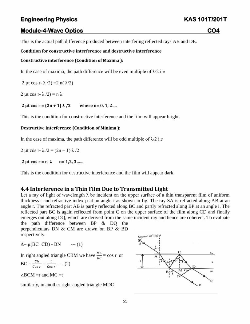
105
PHYSICS Module - 1 Relativistic Mechanics: [8] Frame of reference, Inertial & non-inertial frames, Galilean transformations, Michelson- Morley experiment, Postulates of special theory of relativity, Lorentz transformations, Length contraction, Time dilation, Velocity addition theorem, Variation of mass with velocity, Einstein‟s mass energy relation, Relativistic relation between energy and momentum, Massless particle. Module- 2 Electromagnetic Field Theory: [8] Continuity equation for current density, Displacement current, Modifying equation for the curl of magnetic field to satisfy continuity equation, Maxwell‟s equations in vacuum and in non conducting medium, Energy in an electromagnetic field, Poynting vector and Poynting theorem, Plane electromagnetic waves in vacuum and their transverse nature. Relation between electric and magnetic fields of an electromagnetic wave, Energy and momentum carried by electromagnetic waves, Resultant pressure, Skin depth. Module- 3 Quantum Mechanics: [8] Black body radiation, Stefan‟s law, Wien‟s law, Rayleigh-Jeans law and Planck‟s law, Wave particle duality, Matter waves, Time-dependent and time-independent Schrodinger wave equation, Born interpretation of wave function, Solution to stationary state Schrodinger wave equation for one-Dimensional particle in a box, Compton effect. Module- 4 Wave Optics: [10] Coherent sources, Interference in uniform and wedge shaped thin films, Necessity of extended sources, Newton‟s Rings and its applications. Fraunhoffer diffraction at single slit and at double slit, absent spectra, Diffraction grating, Spectra with grating, Dispersive power, Resolving power of grating, Rayleigh‟s criterion of resolution, Resolving power of grating. Module- 5Fibre Optics & Laser: [10] Fibre Optics: Introduction to fibre optics, Acceptance angle, Numerical aperture, Normalized frequency, Classification of fibre, Attenuation and Dispersion in optical fibres. Laser: Absorption of radiation, Spontaneous and stimulated emission of radiation, Einstein‟s coefficients, Population inversion, Various levels of Laser, Ruby Laser, He-Ne Laser, Laser applications. Course Outcomes: 1. To solve the classical and wave mechanics problems 2. To develop the understanding of laws of thermodynamics and their application in various processes 3. To formulate and solve the engineering problems on Electromagnetism & Electromagnetic Field Theory 4. To aware of limits of classical physics & to apply the ideas in solving the problems in their parent streams Reference Books: 1. Concepts of Modern Physics - AurthurBeiser (Mc-Graw Hill)
Transcript of PHYSICS - Galgotias College of Engineering and Technology

PHYSICS
Module - 1 Relativistic Mechanics [8] Frame of reference Inertial amp non-inertial frames Galilean transformations Michelson-
Morley experiment Postulates of special theory of relativity Lorentz transformations
Length contraction Time dilation Velocity addition theorem Variation of mass with
velocity Einstein‟s mass energy relation Relativistic relation between energy and
momentum Massless particle
Module- 2 Electromagnetic Field Theory [8] Continuity equation for current density Displacement current Modifying equation for the curl of magnetic field to satisfy continuity equation Maxwell‟s equations in vacuum and in non conducting medium Energy in an electromagnetic field Poynting vector and Poynting theorem Plane electromagnetic waves in vacuum and their transverse nature Relation between electric and magnetic fields of an electromagnetic wave Energy and momentum carried by electromagnetic waves Resultant pressure Skin depth
Module- 3 Quantum Mechanics [8] Black body radiation Stefan‟s law Wien‟s law Rayleigh-Jeans law and Planck‟s law Wave particle duality Matter waves Time-dependent and time-independent Schrodinger wave equation Born interpretation of wave function Solution to stationary state Schrodinger wave equation for one-Dimensional particle in a box Compton effect
Module- 4 Wave Optics [10] Coherent sources Interference in uniform and wedge shaped thin films Necessity of extended sources Newton‟s Rings and its applications Fraunhoffer diffraction at single slit and at double slit absent spectra Diffraction grating Spectra with grating Dispersive power Resolving power of grating Rayleigh‟s criterion of resolution Resolving power of grating
Module- 5Fibre Optics amp Laser [10] Fibre Optics Introduction to fibre optics Acceptance angle Numerical aperture Normalized frequency Classification of fibre Attenuation and Dispersion in optical fibres Laser Absorption of radiation Spontaneous and stimulated emission of radiation Einstein‟s coefficients Population inversion Various levels of Laser Ruby Laser He-Ne Laser Laser applications
Course Outcomes
1 To solve the classical and wave mechanics problems 2 To develop the understanding of laws of thermodynamics and their application
in various processes 3 To formulate and solve the engineering problems on Electromagnetism
amp Electromagnetic Field Theory 4 To aware of limits of classical physics amp to apply the ideas in solving the problems in
their parent streams
Reference Books 1 Concepts of Modern Physics - AurthurBeiser (Mc-Graw Hill)
user
Textbox
ENGINEERING PHYSICS13 (KAS 101T201T)
Program Outcomes (POrsquos) relevant to the course
PO1 Engineering knowledge Apply the knowledge of mathematics science engineering fundamentals
and an engineering specialization to the solution of complex engineering problems
PO2 Problem analysis Identify formulate review research literature and analyze complex engineering
problems reaching substantiated conclusions using first principles of mathematics natural sciences
and engineering sciences
PO3 Designdevelopment of solutions Design solutions for complex engineering problems and design
system components or processes that meet the specified needs with appropriate consideration for
the public health and safety and the cultural societal and environmental considerations
PO4 Conduct investigations of complex problems Use research-based knowledge and research
methods including design of experiments analysis and interpretation of data and synthesis of the
information to provide valid conclusions
PO5 Modern tool usage Create select and apply appropriate techniques resources and modern
engineering and it tools including prediction and modeling to complex engineering activities with an
understanding of the limitations
PO6 The engineer and society Apply reasoning informed by the contextual knowledge to assess
societal health safety legal and cultural issues and the consequent responsibilities relevant to the
professional engineering practice
PO7 Environment and sustainability Understand the impact of the professional engineering solutions
in societal and environmental contexts and demonstrate the knowledge of and need for
sustainable development
PO8 Ethics Apply ethical principles and commit to professional ethics and responsibilities and norms of
the engineering practice
PO9 Individual and team work Function effectively as an individual and as a member or leader in
diverse teams and in multidisciplinary settings
PO10 Communications Communicate effectively on complex engineering activities with the engineering
community and with society at large such as being able to comprehend and write effective reports
and design documentation make effective presentations and give and receive clear instructions
PO11 Project management and finance Demonstrate knowledge and understanding of the engineering
and management principles and apply these to onersquos own work as a member and leader in a team
to manage projects and in multidisciplinary environments
PO12 Life-long learning Recognize the need for and have the preparation and ability to engage in
independent and life-long learning in the broadest context of technological change
COURSE OUTCOMES (COs) Engineering Physics (KAS-101T201T)
YEAR OF STUDY 2020-21
Course
outcomes Statement (On completion of this course the student will be able to -)
CO1 Understand the basics of relativistic mechanics(K2)
CO2 Develop EM-wave equations using Maxwellrsquos equations(K1)
CO3 Understand the concepts of quantum mechanics(K2)
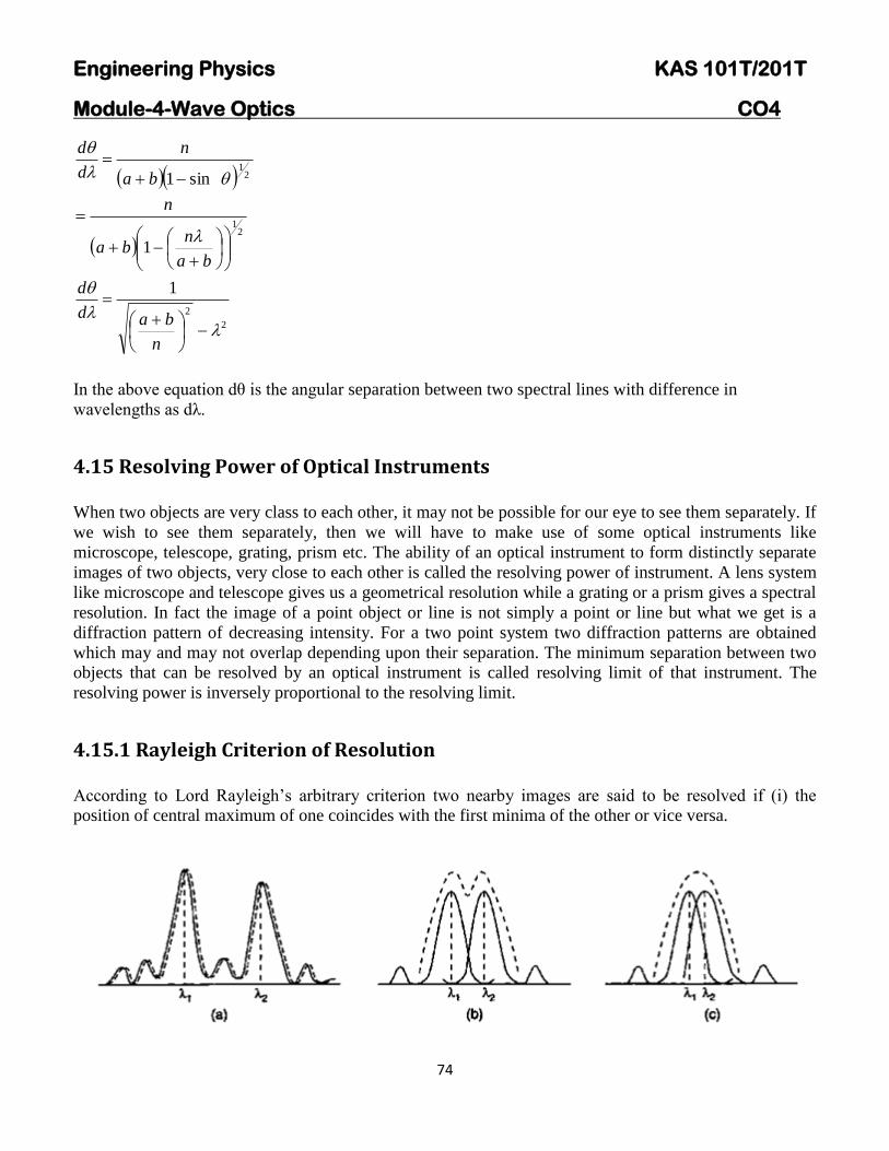
CO4 Describe the various phenomena of light and its applications in different fields(K1)
CO5 Comprehend the concepts and applications of fiber optics and LASER(K2)
Mapping of Course Outcomes with Program Outcomes (CO-PO Mapping)
1 Slight ( low) 2 Moderate ( medium) 3 Substantial (high)
COsPOs PO1 PO2 PO3 PO4 PO5 PO6 PO7 PO8 PO9 PO10 PO11 PO12
CO1 3 3 3
CO2 3 3 3 3
CO3 3 3 3
CO4 2 3
CO5 3 3 3
KAS-
101T201T
3 3 3 3
Engineering Physics KAS 101T201T
Module-1-Relativistic Mechanics CO1
1
11 Introduction of Newtonian Mechanics The universe in which we live is full of dynamic objects Nothing is static here Starting from giant stars
to tiny electrons everything is dynamic This dynamicity of universal objects leads to variety of
interactions events and happenings The curiosity of human beingscientist to know about these events
and laws which governs them Mechanics is the branch of Physics which is mainly concerned with the
study of mobile bodies and their interactions
A real breakthrough in this direction was made my Newton in 1664 by presenting the law of linear motion
of bodies Over two hundred years these laws were considered to be perfect and capable of explaining
everything of nature
12 Frames of Reference The dynamicity of universal objects leads to variety of interactions between these objects leading to
various happenings These happenings are termed as events The relevant data about an event is recorded
by some person or instrument which is known as ldquoObserverrdquo
The motion of material body can only described relative to some other object As such to locate the
position of a particle or event we need a coordinate system which is at rest with respect to the observer
Such a coordinate system is referred as frame of reference or observers frame of reference
ldquoA reference frame is a space or region in which we are making observation and measuring
physical(dynamical) quantities such as velocity and
acceleration of an object(event)rdquo or
ldquoA frame of reference is a three dimensional coordinate
system relative to which described the position and
motion(velocity and acceleration) of a body(object)rdquo
Fig11 represents a frame of reference(S) an object be
situated at point P have co-ordinate ie
P( ) measured by an Observer(O) Where be the time
of measurement of the co-ordinate of an object Observers in
different frame of references may describe same event in
different way
Example- takes a point on the rim of a moving wheel of cycle for an observer sitting at the center of the
wheel the path of the point will be a circle However For an observer standing on the ground the path of
the point will appear as cycloid
Fig 11 frame of reference
Engineering Physics KAS 101T201T
Module-1-Relativistic Mechanics CO1
2
There are two types of frames of reference
1 Inertial or non-accelerating frames of reference
2 Non-inertial or accelerating frames of reference
The frame of reference in which Newtons laws of motion hold good is treated as inertial frame of
reference However the frame of reference in which Newtons laws of motion not hold good is treated as
non-inertial frame of reference Earth is non-inertial frame of reference because it has acceleration due
to spin motion about its axis and orbital motion around the sun
13 Galilean Transformations The Galilean transformations equations are used to transform the coordinates of position and time from
one inertial frame to the other The equations relating the coordinates of a particle in two inertial frames
are called as Galilean transformations Consider the two inertial frames of reference F and F Let the
frame F is moving with constant velocity v with reference to frame F The frames F and F are shown in
Fig1
Let some event occurs at the point P at any instant of time t The coordinates of point P with respect to
frame F are x y z t and with respect to frame F are x y z t Let at t = t= 0 the origin O of frame F
and O of frame F coincides with one another Also axes x and x are parallel to v Let y and z are parallel
to y and z respectively
From Fig
x=x+ vthelliphelliphelliphelliphelliphelliphelliphelliphelliphelliphellip(1)
x= x - vthelliphelliphelliphelliphelliphelliphelliphelliphelliphelliphellip(2)
As there is no relative motion along y and z-
axes we can writ
y=yhelliphellip(3)
z=zhelliphellip(4) and t=thelliphellip(5)
These equations are called as Galilean
transformation equations The inverse Galilean transformation can be written as
x=x + vt y=y z=z and t=t
Hence transformation in position is variant only along the direction of motion of the frame and remaining
dimensions( y and z) are unchanged under Galilean Transformation At that era scientist were assumed
time should be absolute
Engineering Physics KAS 101T201T
Module-1-Relativistic Mechanics CO1
3
b) Transformation in velocities components The conversion of velocity components measured in frame F into their equivalent components in the
frame F can be known by differential Equation (1) with respect to time we get
ux=
=
( )
hence ux= ux-V
Similarly from Equation (3) and (4) we can write
uy= uy and uz= uz
In vector form
Hence transformation in velocity is variant only along the direction of motion of the frame and remaining
dimensions( along y and z) are unchanged under Galilean Transformation
c) Transformation in acceleration components
The acceleration components can be derived by differentiating velocity equations with respect to
time
ax=
( )
ax= ax
In vector form a = a
This shows that in all inertial reference frames a body will be observed to have the same acceleration
Hence acceleration are invariant under Galilean Transformation
Failures of Galilean transformation According to Galilean transformations the laws of mechanics are invariant But under Galilean
transformations the fundamental equations of electricity and magnetism have very different
forms
Also if we measure the speed of light c along x-direction in the frame F and then in the frame F
the value comes to be c = c ndash vx But according to special theory of relativity the speed of light c
is same in all inertial frames
14 Michelson-Morley Experiment ldquoThe objective of Michelson - Morley experiment was to detect the existence of stationary medium ether
(stationary frame of reference ie ether frame)rdquo which was assumed to be required for the propagation of
the light in the space
u=u ndash v
Engineering Physics KAS 101T201T
Module-1-Relativistic Mechanics CO1
4
In order to detect the change in velocity of light due to relative motion between earth and hypothetical
medium ether Michelson and Morley performed an experiment which is discussed below The
experimental arrangement is shown in Fig
Light from a monochromatic source S falls on the semi-silvered glass plate G inclined at an angle 45deg to
the beam It is divided into two parts by the semi silvered surface one ray 1 which travels towards mirror
M1 and other is transmitted ray 2 towards mirror M2 These two rays fall normally on mirrors M1 and M2
respectively and are reflected back along their original paths and meet at point G and enter in telescope In
telescope interference pattern is obtained
If the apparatus is at rest in ether the two reflected rays would take equal time to return the glass plate G
But actually the whole apparatus is moving along with the earth with a velocity say v Due to motion of
earth the optical path traversed by both the rays are not the same Thus the time taken by the two rays to
travel to the mirrors and back to G will be different in this case
Let the mirrors M1 and M2 are at equal distance l from the glass plate G Further let c and v be the
velocities at light and apparatus or earth respectively It is clear from Fig that the reflected ray 1 from
glass plate G strikes the mirror M1at A and not at A due to the motion of the earth
The total path of the ray from G to A and back will be GAG
there4 From Δ GAD (GA)2=(AA)
2+ (AD)
2(1) As (GD =AA)
If t be the time taken by the ray to move from G to A then from Equation (1) we have
(c t)2=(v t)
2 + (l)
2
Hence t=
radic
If t1 be the time taken by the ray to travel the whole path GAG then
Engineering Physics KAS 101T201T
Module-1-Relativistic Mechanics CO1
5
t1= 2t =
radic =
(
)
t1=
((
)) helliphelliphelliphelliphelliphellip(2) Using Binomial Theorem
Now in case of transmitted ray 2 which is moving longitudinally towards mirror M2 It has a velocity (c ndash
v) relative to the apparatus when it is moving from G to B During its return journey its velocity relative
to apparatus is (c + v) If t2 be the total time taken by the longitudinal ray to reach G then
T2=
( )
( ) after solving
t2=
((
)) helliphelliphelliphelliphelliphellip(3)
Thus the difference in times of travel of longitudinal and transverse journeys is
Δt = t2-t1 = =
((
))
((
))
Δt =
helliphelliphelliphelliphelliphellip(4)
The optical path difference between two rays is given as
Optical path difference (Δ) =Velocity times t = c x Δt
= c x =
Δ =
helliphelliphelliphelliphelliphellip(5)
If λ is the wavelength of light used then path difference in terms of wavelength is =
λ
Michelson-Morley perform the experiment in two steps First by setting as shown in fig and secondly by
turning the apparatus through 900 Now the path difference is in opposite direction ie path difference is
-
λ
Hence total fringe shift ΔN =
Michelson and Morley using l=11 m λ= 5800 x 10-10
m v= 3 x 10⁴ msec and c= 3 x 10
8 msec
there4 Change in fringe shift ΔN =
λ substitute all these values
=037 fringe
Engineering Physics KAS 101T201T
Module-1-Relativistic Mechanics CO1
6
But the experimental were detecting no fringe shift So there was some problem in theory calculation and
is a negative result The conclusion drawn from the Michelson-Morley experiment is that there is no
existence of stationary medium ether in space
Negative results of Michelson - Morley experiment 1 Ether drag hypothesis In Michelson - Morley experiment it is explained that there is no relative
motion between the ether and earth Whereas the moving earth drags ether alone with its motion
so the relative velocity of ether and earth will be zero
2 Lorentz-Fitzgerald Hypothesis Lorentz told that the length of the arm (distance between the pale
and the mirror M2) towards the transmitted side should be L(radic1 ndash v2c
2) but not L If this is taken
then theory and experimental will get matched But this hypothesis is discarded as there was no
proof for this
3 Constancy of Velocity of light In Michelson - Morley experiment the null shift in fringes was
observed According to Einstein the velocity of light is constant it is independent of frame of
reference source and observer
Einstein special theory of Relativity (STR)
Einstein gave his special theory of relativity (STR) on the basis of M-M experiment
Einsteinrsquos First Postulate of theory of relativity
All the laws of physics are same (or have the same form) in all the inertial frames of reference
moving with uniform velocity with respect to each other (This postulate is also called the law of
equivalence)
Einsteinrsquos second Postulate of theory of relativity
The speed of light is constant in free space or in vacuum in all the inertial frames of reference
moving with uniform velocity with respect to each other (This postulate is also called the law of
constancy)
15 Lorentz Transformation Equations
Consider the two observers O and O at the origin of the inertial frame of reference F and F respectively
as shown in Fig Let at time t = t = 0 the two coordinate systems coincide initially Let a pulse of light is
flashed at time t = 0 from the origin which spreads out in the space and at the same time the frame F starts
moving with constant velocity v along positive X-direction relative to the frame F This pulse of light
reaches at point P whose coordinates of position and time are (x y z t) and (xy z t) measured by the
observer O and O respectively Therefore the transformation
equations of x and x can be given as
x=k (x ndash v t)helliphelliphelliphelliphelliphelliphelliphelliphellip(1)
Where k is the proportionality constant and is independent of
x and t
Engineering Physics KAS 101T201T
Module-1-Relativistic Mechanics CO1
7
The inverse relation can be given as
x=k (x + v t) helliphelliphelliphelliphelliphelliphellip (2)
As t and t are not equal substitute the value of x from Equation (1) in Equation (2)
x=k [k (x ndash vt) + vt] or
=( )
t=
or t=
(
) helliphelliphelliphelliphelliphelliphelliphelliphellip(3)
According to second postulate of special theory of relativity the speed of light c remains constant
Therefore the velocity of pulse of light which spreads out from the common origin observed by observer
O and O should be same
there4 x=c t and x = cthelliphelliphelliphelliphelliphelliphelliphelliphelliphelliphelliphelliphelliphelliphellip(4)
Substitute the values of x and x from Equation (4) in Equation (1) and (2) we get
ct=k (x ndash v t) = k (ct ndash v t) or ct=kt (c ndash v) (5)
and similarly ct=k t (c + v) (6)
Multiplying Equation (5) and (6) we get
c2 t t=k
2t t (c
2 ndash v
2) hence
after solving k=
radic
(7)
Hence equation (7) substitute in equation (1) then Lorentz transformation in position will be
x=
radic
y=y z=z
Calculation of Time equation (7) substitute in equation (3)
t=
(
)
From equation ( 7)
or
then above equation becomes
t=
=
or t= (
)
Engineering Physics KAS 101T201T
Module-1-Relativistic Mechanics CO1
8
Therefore t=
radic
Hence the Lorentz transformation equations becomes
x=
radic
y=y z=z and t=
radic
Under the condition Lorentz transformation equation can be converted in to Galilean
Transformation
x=x -vt y=y z=z and t=t
16 Applications of Lorentz Transformation
161 Length contraction Consider a rod at rest in a moving frame of reference F moving along x-direction with constant velocity
v relative to the fixed frame of reference F as shown in Fig
The observer in the frame F measures the length
of rod AB at any instant of time t This length Lo
measured in the system in which the rod is at rest
is called proper length therefore Lo is given as
Lo= x2- x1 helliphelliphelliphelliphelliphelliphelliphelliphelliphelliphellip(1)
Where x1 and x2 are the coordinates of the two
ends of the rod at any instant At the same time
the length of the rod is measured by an observer
O in his frame say L then
L= x2- x1 helliphelliphelliphelliphelliphelliphelliphelliphelliphelliphellip(2)
Where x1 and x2 are the coordinates of the rod AB
respectively with respect to the frame F According to Lorentz transformation equation
x1=
radic
and x2=
radic
Hence x2- x1=
radic
By using Equations (1) and (2) we can write
Lo=
radic
Engineering Physics KAS 101T201T
Module-1-Relativistic Mechanics CO1
9
Hence L=Lo radic
helliphelliphelliphelliphelliphelliphellip(3)
From this equation Thus the length of the rod is contracted by a factor radic
as measured by observer in
stationary frame F
Special Case
If v ltltlt c then v2c
2 will be negligible in Loradic
and it can be neglected
Then equation (3) becomes L = LO
Percentage of length contraction=
162 Time dilation Let there are two inertial frames of references F and F F is the stationary frame of reference and F is the
moving frame of reference At time t=trsquo=0 that is in the start they are at the same position that is
Observers O and Orsquo coincides After that F frame starts moving with a uniform velocity v along x axis
Let a clock is placed in the frame F The time coordinate of the initial time of the clock will be t1
according to the observer in S and the time coordinate of the final tick (time) will be will be t2 according
to same observer
The time coordinate of the initial time of the clock will be t1 according to the observer in F and the time
coordinate of the final tick (time) will be will be t2 according to same observer
Therefore the time of the object as seen by
observer O in F at the position xrsquo will be
to = trsquo2 ndash trsquo1 helliphelliphelliphelliphelliphelliphelliphelliphelliphelliphelliphellip(1)
The time trsquo is called the proper time of the event
The apparent or dilated time of the same event
from frame S at the same position x will be
t = t2 ndash t1 helliphelliphelliphelliphelliphelliphelliphelliphelliphelliphelliphellip(2)
Now use Lorentz inverse transformation
equations for that is
t1 =
radic
helliphelliphelliphelliphelliphelliphelliphellip (3)
t2 =
radic
helliphelliphelliphelliphelliphelliphelliphellip (3)
Engineering Physics KAS 101T201T
Module-1-Relativistic Mechanics CO1
10
By putting equations (3) and (4) in equation (2) and solving we get
t =
radic
Substitute equation (1) in above equation
t =
radic
This is the relation of the time dilation
Special Case
If v ltltlt c then v2c
2 will be negligible in
radic
and it can be neglected
Then t = to
Experimental evidence The time dilation is real effect can be verified by the following experiment In
1971 NASA conducted one experiment in which JC Hafele as astronomer and RF Keating a physicist
circled the earth twice in a jet plane once from east to west for two days and then from west to east for
two days carrying two cesium-beam atomic clocks capable of measuring time to a nanosecond After the
trip the clocks were compared with identical clocks The clocks on the plane lost 59 10 ns during their
eastward trip and gained 273 7 ns during the westward tripThis results shows that time dilation is real
effect
163 Relativistic Addition of Velocities One of the consequences of the Lorentz transformation equations is the counter-intuitive ldquovelocity
addition theoremrdquo Consider an inertial frame Srsquo moving with uniform velocity v relative to stationary
observer S along the positive direction of X- axis Suppose a particle is also moving along the positive
direction of X-axis If the particle moves through a distance dx in time interval dt in frame S then
velocity of the particle as measured by an observer in this frame is given by
(1)
To an observer in Srsquo frame let the velocity be (by definition)
(2)
Now we have the Lorentz transformation equations
radic(
)
and
radic(
)
(3)
Taking differentials of above equations we get
Engineering Physics KAS 101T201T
Module-1-Relativistic Mechanics CO1
11
and
radic( ) (4)
Using eq (4) in eq(2) we get
(
)
( ) (5)
Or
( ) (6)
This is the the relativistic velocity addition formula If the speeds u and v are small compared to the speed
of light above formula reduces to Newtonian velocity addition formula
Inverse of the formula (6) enables us to find velocity of a particle in S frame if it is given in Srsquo frame
(6)
17 Variation of Mass with Velocity In Newtonian physics mass of an object used to be an absolute entity same in all frames One of the
major unusual consequences of relativity was relativity of mass In the framework of relativity it can be
shown that mass of an object increases with its velocity We have the following equation expressing the
variation of mass with velocity
radic( ) (1)
Where is the mass of the object at rest known as rest mass and is its velocity relative to observer
As it is clear from above equation if in agreement with common experience
Derivation
We use relativistic law of momentum conservation to arrive at eq (1) Consider two inertial frames S and
Srsquo Srsquo moving with respect to S with velocity v along positive X-axis Let two masses and are
moving with velocities ursquo and ndashursquo with respect to moving frame Srsquo
Now let us analyse the collision between two bodies with respect to frame S If u1 and u2
are velocities of two masses with respect to frame S then from velocity addition theorem
and
(2)
Engineering Physics KAS 101T201T
Module-1-Relativistic Mechanics CO1
12
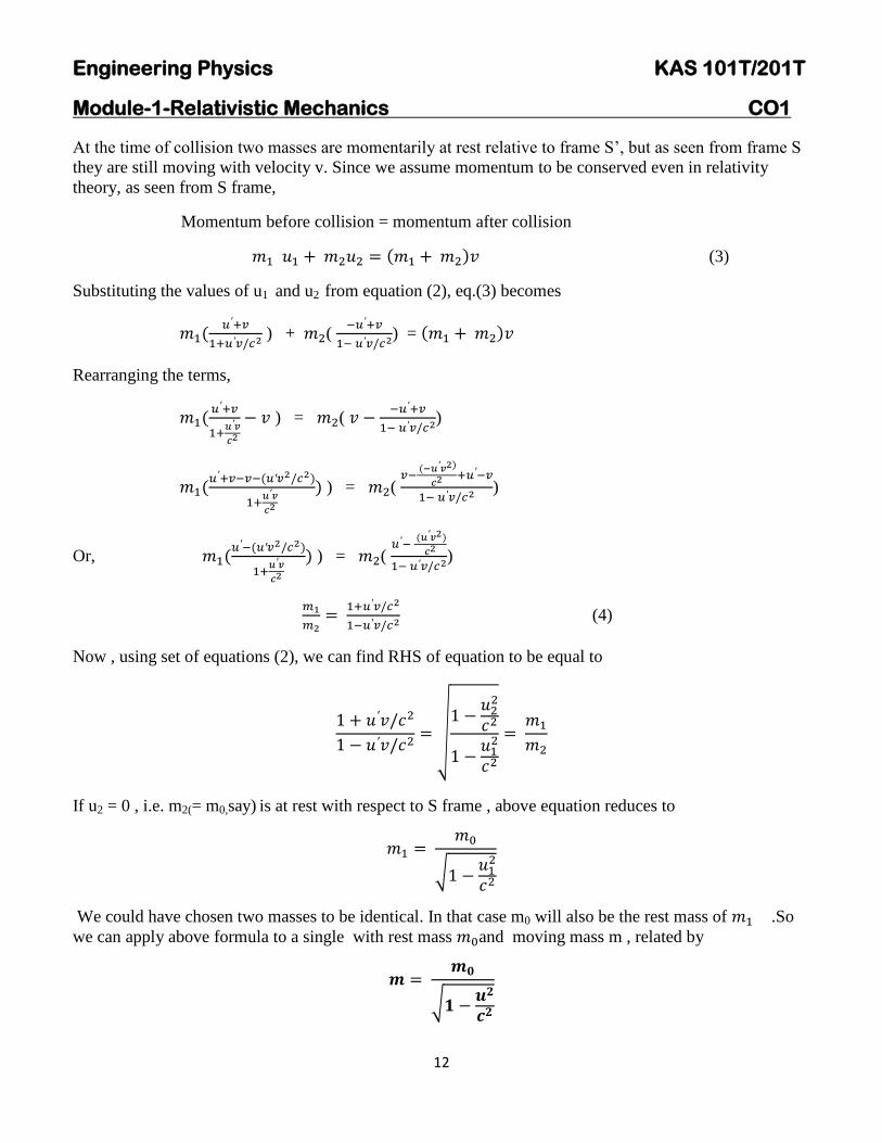
At the time of collision two masses are momentarily at rest relative to frame Srsquo but as seen from frame S
they are still moving with velocity v Since we assume momentum to be conserved even in relativity
theory as seen from S frame
Momentum before collision = momentum after collision
( ) (3)
Substituting the values of u1 and u2 from equation (2) eq(3) becomes
(
) + (
) = ( )
Rearranging the terms
(
) = (
)
( ( )
) ) = (
( )
)
Or ( ( )
) ) = (
( )
)
(4)
Now using set of equations (2) we can find RHS of equation to be equal to
radic
If u2 = 0 ie m2(= m0say) is at rest with respect to S frame above equation reduces to
radic
We could have chosen two masses to be identical In that case m0 will also be the rest mass of So
we can apply above formula to a single with rest mass and moving mass m related by
radic
Engineering Physics KAS 101T201T
Module-1-Relativistic Mechanics CO1
13
This shows that mass of a body increases with its velocity
18 Mass- Energy Equivalence In Newtonian Physics mass and energy are assumed to be quite different entities There is no mechanism
in Newtonian set up how mass and energy can be converted into each other Like many other it is one of
unusual consequences of special relativity that mass and energy are inter-convertible into each other and
hence are equivalent
Einsteinrsquos Mass- energy relation ( ) (Derivation)
Consider a particle of mass m acted upon by a force F in the same direction as its velocity v If F
displaces the particle through distance ds then work done dW is stored as kinetic energy of the particle
dK therefore
(1)
But from Newtonrsquos law
( )
(2)
Using (2) in (1)
Or (3)
Now we have
radic
(
) (4)
Taking the differential
( )(
) (
)
(
)
But ( )
( )
(
)
Or
( )
or ( ) (5)
Using eq (5) in eq (3)
Engineering Physics KAS 101T201T
Module-1-Relativistic Mechanics CO1
14
( )
Let the change in kinetic energy of the particle be K as its mass changes from rest mass to to
effective mass m then
int int
( ) = (
radic
)
This is the relativistic expression for kinetic energy of a particle It says that kinetic energy of a particle is
due to the increase in mass of the particle on account of its relative motion and is equal to the product of
the gain in mass and square of the velocity of light can be regarded as the rest energy of the
particle of rest mass The total energy E of a moving particle is the sum of kinetic energy and its rest
mass energy
( )
Or
This is the celebrated mass- energy equivalence relation This equation is so famous that even common
men identify Einstein with it
Significance This equation represents that energy can neither be created nor be destroyed but it can
change its form
Evidence show its validity
First verification of the was made by Cock-croft and Walton
(70166 amu) (10076 amu) (40026 amu)
Mass defect = (70166 amu+10076 amu) -2x (40028 amu)
=00186 amu
= 00186 x 166 X 10-27
kg
= 00186 x 166 X 10-27
x ( )
=
=( )
( )
=
Engineering Physics KAS 101T201T
Module-1-Relativistic Mechanics CO1
15
( a huge amount of energy release)
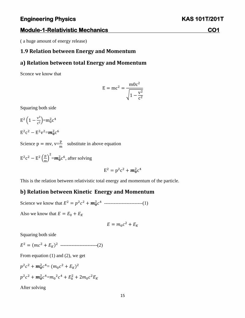
19 Relation between Energy and Momentum
a) Relation between total Energy and Momentum
Sconce we know that
radic
Squaring both side
(
)=
=
Science =
substitute in above equation
(
)
= after solving
This is the relation between relativistic total energy and momentum of the particle
b) Relation between Kinetic Energy and Momentum
Science we know that ------------------------(1)
Also we know that
Squaring both side
( ) -----------------------(2)
From equation (1) and (2) we get
= (
)
=
After solving
Engineering Physics KAS 101T201T
Module-1-Relativistic Mechanics CO1
16
radic
Where = kinetic energy
110 Mass-less Particle Zero Rest Mass Particles A particle which has zero rest mass( ) is called massless particle
We have the energy-momentum relation
radic ( ) (1)
For a massless particle
Therefore or (2)
But therefore
Which implies
This says that a massless particles always move with the speed of light Energy and momentum of a
massless particle is given by equation (2) Massless particles can exist only as long as the move at the
speed of light Examples are photon neutrinos and theoretically predicted gravitons
Numerical Problems
Question 1 Show that the distance between any two points in two inertial frame is invariant under
Galilean transformation
Answer Consider two frame of reference S and frame moving with constant velocity relative
to frame S in positive X-direction
Point A and B placed in frame S and their co-ordinate relative O are ( ) and ( )
After time the coordinate of A and B relative to observer from frame will be ( )
and( )
Using Galilean Transformation
and
and
Engineering Physics KAS 101T201T
Module-1-Relativistic Mechanics CO1
17
Now distance between two points from frame will be
=radic( ) ( ) ( )
Substitute all values then
=radic( ) ( ) ( )
After simplification
=radic( ) ( ) ( ) ie
=
This show that distance between two points is invariant under Galilean Transformation
Question 2 Show that the relativistic form of Newtonrsquos second law when is parallel to
=
(
)
Answer Science we know that
=
(
radic
)=[ ( (
)
)]
= [
(
)
(
) (
)
(
)]
=
[(
)
(
)
]
=
(
)
+
=
(
)
it is relativistic Newtonrsquos second law
Engineering Physics KAS 101T201T
Module-1-Relativistic Mechanics CO1
18
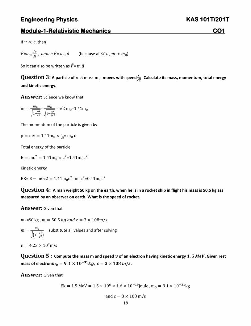
If then
=
= (because at )
So it can also be written as =
Question 3 A particle of rest mass moves with speed
radic Calculate its mass momentum total energy
and kinetic energy
Answer Science we know that
radic
=
radic
= radic =141
The momentum of the particle is given by
radic =
Total energy of the particle
=
Kinetic energy
= -
=
Question 4 A man weight 50 kg on the earth when he is in a rocket ship in flight his mass is 505 kg ass
measured by an observer on earth What is the speed of rocket
Answer Given that
=50 kg
radic(
)
substitute all values and after solving
ms
Question 5 Compute the mass m and speed of an electron having kinetic energy Given rest
mass of electron
Answer Given that
Engineering Physics KAS 101T201T
Module-1-Relativistic Mechanics CO1
19
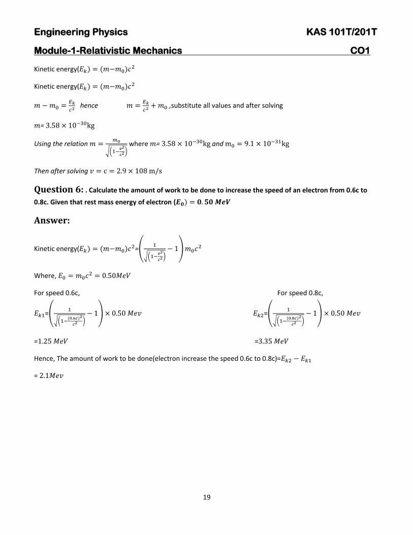
Kinetic energy( ) ( )
Kinetic energy( ) ( )
hence
substitute all values and after solving
=
Using the relation
radic(
)
where = and
Then after solving
Question 6 Calculate the amount of work to be done to increase the speed of an electron from 06c to
08c Given that rest mass energy of electron ( )
Answer
Kinetic energy( ) ( ) =(
radic(
)
)
Where
For speed 06c For speed 08c
=(
radic( ( )
)
) =(
radic( ( )
)
)
= =
Hence The amount of work to be done(electron increase the speed 06c to 08c)=
=
Engineering Physics KAS 101T201T
Module-2-Electromagnetic Field Theory CO2
20
21 Continuity equation for current density Statement Equation of continuity represents the law of conservation of charge The charge flowing out
through a closed surface from some volume is equal to the rate of decrease of charge within the volume
hellip (1)
Where I is current flowing out through the surface of a volume and
is the rate of decrease of charge
within the volume
Again we know ∯ and q= intintintρdv
where J is the Conduction current density an ρ is the volume charge density
Substituting the expression of I and q in equation (1)
∯ ∭
hellip (2)
Now applying Gaussrsquos Divergence Theorem to LHS of above equation
∭ ∭
As the two volume integrals are equal so their integrands are also equal
Thus
This is continuity equation for time varying fields
Equation of Continuity for Steady Currents As ρ does not vary with time for steady currents that is
So
This is the continuity equation for steady currents
Engineering Physics KAS 101T201T
Module-2-Electromagnetic Field Theory CO2
21
22 Differential form of Maxwellrsquos equations
221 First equation (Gauss Law of Electrostatic)
Gauss law of electrostatic states that the total electric flux E coming out from a closed surface is equal to
1ε0 times the net charge enclosed by the surface ie ∯
∯ =intintintρdv hellip (1)
Applying Gaussrsquos Divergence theorem to change LHS of equation (1) ∯ =intv (nablaD) dv
Using this equation in equation (1) we will get
intintint (nablaD)dv=intintintρdv
As two volume integrals are equal so their integrands are also equal
Thus nablaD=ρ hellip (2)
The above equation is the Differential form of Maxwellrsquos first equation
222 Second equation(Gauss Law of Magnetostatic)
Gauss law of magnetostatic states that the total magnetic flux φm coming out through surface of a volume
is always equal to zero
φm=∯ hellip(3)
Applying Gaussrsquos Divergence theorem ∯ =intintint(nablaB)dv
Putting this in equation (3) intintint (nablaB)dv =0
Thus nablaB=0 hellip(4)
This equation (4) is differential form of Maxwellrsquos second equation
223 Third Equation(Faradayrsquos Law of Electromagnetic Induction)
1 It states that if there is a change of magnetic flux linked with a circuit then electromotive force (emf) is
induced in the circuit This induced emf lasts as long as the change in magnetic flux continues
Engineering Physics KAS 101T201T
Module-2-Electromagnetic Field Theory CO2
22
2 The magnitude of induced emf is equal to the rate of change of magnetic flux linked with the circuit
Therefore induced emf
hellip(5)
Where φm= intintBds hellip(6)
Here negative sign indicates the induced emf set up a current in such a direction that the magnetic effect
produced by it opposes the cause producing it
Again we know emf is the closed line integral of the non-conservative electric field generated by the
battery
That is emf=∮ hellip(7)
Putting equations (6) and (7) in equation (5) we get
∮ = ndash intint
ds hellip(8)
Using Stokersquos theorem to the LHS of equations (8) ∮ = intint (nabla x E)ds
Substituting above equation in equation (8) we get
intint (nabla x E)dS = -intint
ds
Two surface integral are equal only when their integrands are equal
Thus nabla x E = ndash
hellip(9)
This is the differential form of Maxwellrsquos 3rd
equation
224 Forth Equation (Modified Amperersquos Circuital Law)
To come to the Maxwellrsquos 4th
equation let us first discuss Amperersquos circuital law
Amperersquos circuital law This law states that the line integral of the magnetic field H around any closed
path or circuit is equal to the current enclosed by that path
That is ∮ =I
Engineering Physics KAS 101T201T
Module-2-Electromagnetic Field Theory CO2
23
If J is the current density then I=intintJds
This implies that ∮ =intintJds hellip(10)
Applying Stokersquos theorem to LHS of above equation ∮ =intint(nablaxH)ds
Substituting above equation in equation (10) we will get intint(nablaxH)ds =intintJds
Two surface integrals are equal only if their integrands are equal
Thus nablax H=J hellip(11)
This is the differential form of Amperersquos circuital Law for steady currents
Now taking divergence on both side of equation (10) nabla(nablaxH)= nablaJ
As divergence of the curl of a vector is always zero therefore nabla(nablaxH)=0
It means nablaJ=0
Now this is continuity equation for steady current but not for time varying fields as equation of
continuity for time varying fields is
So Amperersquos circuital law is incomplete valid only for steady state current This is the reason that led
Maxwell to modify Amperersquos circuital law
Modification of Amperersquos circuital law Maxwell modified Amperersquos law by giving the concept of
displacement current and displacement current density for time varying fields
He considered that equation (10) for time varying fields can be written as nablaxH=J + Jd hellip (12)
By taking divergence on both side of equation (12) we will get nabla (nabla xH)= nablaJ+ nablaJd
As the divergence of curl of a vector is always zero therefore nabla (nabla xH)= 0
So nabla (J+Jd)=0 Or nabla J= -nablaJd
But from equation of continuity for time varying fields
Engineering Physics KAS 101T201T
Module-2-Electromagnetic Field Theory CO2
24
From the above two equations of j we get
nabla Jd = ( )
hellip (13)
As from Maxwellrsquos first equation nablaD=ρ
Now from equation (13) we can write
Using the above equation in equation (12) we get
nabla x H=J +
hellip(14)
Here
=Displacement current density
The equation (14) is the Differential form of Maxwellrsquos fourth equation or Modified Amperersquos circuital
law
23 Integral form of Maxwellrsquos equations
231 First Equation
Gauss law of electrostatic states that the total electric flux E coming out from a closed surface is
equal to 1ε0 times the net charge enclosed by the surface ie
∯ hellip(1)
Let ρ is the volume charge density distributed over a volume V
Therefore q=int ρ dv
So ∯
hellip(2)
This equation is the integral form of Maxwellrsquos first equation or Gaussrsquos law in electrostatics
232 Second equation
Gauss law of magnetostatic states that the total magnetic flux φm coming out through surface of a volume
is always equal to zero ie
φm=∯ hellip(3)
Engineering Physics KAS 101T201T
Module-2-Electromagnetic Field Theory CO2
25
The above equation is the intergal form of Maxwellrsquos second equation
The above equation also suggest that magnetic monopole does not exist
233 Third Equation
1 It states that if there is a change of magnetic flux linked with a circuit then electromotive force (emf) is
induced in the circuit This induced emf lasts as long as the change in magnetic flux continues
2 The magnitude of induced emf is equal to the rate of change of magnetic flux linked with the circuit
Therefore induced emf
hellip(4)
Where φm= intintBds hellip(5)
Here negative sign indicates the induced emf set up a current in such a direction that the magnetic effect
produced by it opposes the cause producing it
Again we know emf is the closed line integral of the non-conservative electric field generated by the
battery
That is emf=∮ hellip(6)
Using equations (5) and (6) in equation (4) we get
∮ = ndash intint
ds hellip(7)
The above equation is the integral form of Maxwellrsquos third Equation or Faradayrsquos law of
electromagnetic induction
234 Fourth equation
The line integration of the magnetic field H around a closed path or circuit is equal to the conductions
current plus the time derivative of electric displacement through the surface bounded by the closed path
ie
∮ =∬(
) (8)
The above equation is the integral form of Maxwellrsquos fourth equation
Engineering Physics KAS 101T201T
Module-2-Electromagnetic Field Theory CO2
26
25 Displacement Current
According to Maxwell not only conduction current produces magnetic field but also time varying electric
field produces magnetic field This means that a changing electric field is equivalent to a current which
flows as long as electric filed is changing This is current only in the sense that it produces same magnetic
effect as conduction current does there is no actual flow of electron
If E is the electric field developed between the plates of surface area A Then the displacement current is
given by
26 Electromagnetic wave Equation in Free Space
Now in free space there is no charge so charge density ρ=0 and current will also be zero Thus current
density J is also equal to zero
Hence Maxwellrsquos equation in free space is given by
hellip(1) where ( )
hellip(2)
hellip(3) where ( )
hellip(4) where ( )
261 Maxwellrsquos Electromagnetic wave Equation in Free Space for the field vector E
we take curl on both side of Maxwellrsquos 3rd
equation represented in equation (3)
( )
( ) ( )
[(using vector identity ( ) ( ) ]
Now from equation (1) and (4) in the above equation
Engineering Physics KAS 101T201T
Module-2-Electromagnetic Field Theory CO2
27
(
)
Or
hellip(5)
Similarly we can find an equation for the field vector B when we take the Maxwellrsquos 4th
and repeat the
process of field vector E
hellip(6)
Equation (5) and (6) is the guiding equation for field vector E and B respectively in free space
Thus we can see that time varying electric field produces magnetic field and time varying magnetic field
produces electric filed and follow the above guiding equation Comparing the above equation with the
standard wave equation
-------(7)
Compare equation (6) and (7) we get
radic radic
radic
Because
Hence = c
Hence this field vectors propagates in free space with the speed of light So from here Maxwell
concluded that light is an electromagnetic wave
27 Electromagnetic wave Equation in non-conducting medium
Now in non-conducting medium there is no free charge so current density J and total charge inside the
material is zero so charge density ρ is also equal to zero Maxwellrsquos equation in a non-conducting
medium of permittivity and permeability is reduces to
Engineering Physics KAS 101T201T
Module-2-Electromagnetic Field Theory CO2
28
hellip(1) where ( )
hellip(2)
hellip(3) where ( )
hellip(4) where ( )
271 Maxwellrsquos Electromagnetic wave Equation in Free Space for the field vector E
we take curl on both side of Maxwellrsquos 3rd
equation represented in equation (3)
( )
( ) ( )
[(using vector identity ( ) ( ) ]
Now using equation (1) and (4) in the above equation
(
)
Or
hellip(5)
Similarly we can find an equation for the field vector B when we take the Maxwellrsquos 4th
and repeat the
process of field vector E
hellip(6)
Equation (5) and (6) is the guiding equation for field vector E and B respectively in non-conducting
medium
Comparing the above equation with the standard wave equation
----------(7)
Engineering Physics KAS 101T201T
Module-2-Electromagnetic Field Theory CO2
29
we can see that this field vectors propagate in non-conducting medium with a speed
radic
radic
radic As 119888
radic
For non-magnetic medium 119903=1
So
radic
here radic 119903 119899 is the refractive index of the medium
Hence electromagnetic wave propagate in non-conducting medium with a speed
times the speed of
electromagnetic wave in free space
28 Transverse nature of electromagnetic wave
Science we know that the plane electromagnetic wave equation are
---(1)
---(2)
Solution of these wave equation considering the propagation of the wave in any arbitrary direction of
three dimensional space is given by
( 119903 ) (3)
( 119903 ) hellip(4)
Where E0 and B0 are the amplitudes of electric and magnetic field respectively and is propagation vector
given by = 2πλ = 2πνc = ωc
Now Maxwellrsquos first and second equation in free space is
nabla =0 hellip(5)
nabla hellip(6)
Engineering Physics KAS 101T201T
Module-2-Electromagnetic Field Theory CO2
30
Where nabla
and = 119910 119911
Putting the above expressions in L H S of equation (5)
nabla = (
) ( 119903 ) ------ (7)
Where k ky kz
and 119903 = y
So 119903 = k yky kz
Thus equation (7) can be written as
= (
)( 119910 119911
) exp ί( k yky kz )- +
=
[ exp ί ( k yky k
z )
- +]+
[ 119910exp ί ( k yky k
z )
- +]+
[ 119911
exp ί ( k yky kz )
- +]
=(ί k ) exp ί ( k yky kz )
- + +(ίky) 119910exp ί ( k yky k
z) - + +(ίk
z )
119911 exp ί ( k yky k
z )
- +
= ί[ k + 119910ky+ 119911 k
z] exp ί ( k yky k
z) - +
= ί[( k ky kz )( 119910 119911
)] exp ί ( k yky k
z )
- +
= ί( )exp(( 119903 )= ί
= ί using equation (3)
Now putting the value of in equation (5)
= ί
Or helliphellip (8)
Similarly putting equation (4) in equation (6) we will get hellip(9)
Equation (8) amp (9) suggest that electric and magnetic field vectors are perpendicular to propagation
vector So we can say that electromagnetic waves are transverse in nature
Again using Maxwellrsquos 3rd
and 4th
equations in free space are
hellip(10)
Engineering Physics KAS 101T201T
Module-2-Electromagnetic Field Theory CO2
31
hellip(11)
Now if we put the expression of from equation (3) in above Maxwellrsquos equation (equation No 10) then
we can write
ί [ ] =
( 119903 )]
= -(- ) ( 119903 )
= hellip(12)
Similarly putting the expression of from equation (4) in equation (12) we will get
= - -----(13)
From equation (12) we can say magnetic field vector is perpendicular to both amp and from (13) we
can say Electric field vector is perpendicular to both Thus electric field vector magnetic field
vector and propagation vector are mutually perpendicular to each other
Characteristic Impedance
As amp are perpendicular to each other and amp are mutually perpendicular so from
equation (12)
=
Or
Or
=
νλ = c
Thus
= c
Or
= micro
0 c and 119888
radic
Or
=
radic
= radic
= 37672 Ω
The quantity
= Z
0 = 37672Ω is known as characteristic Impedance or Intrinsic Impedance of free
space
Engineering Physics KAS 101T201T
Module-2-Electromagnetic Field Theory CO2
32
29 Energy in an electromagnetic field
The Energy of electromagnetic Wave is the sum of electric (E) and magnetic (B) field energy
The electric energy per unit volume is given by UE
The magnetic energy per unit volume is given by UB
So the total energy per unit volume in electromagnetic wave is
U =
As
and
radic So U =
+
=
+
= Ɛ0E
2
Therefore energy per unit volume in electromagnetic wave is U = Ɛ0E2
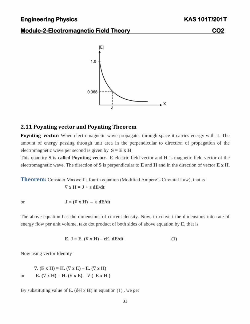
210 Skin Depth
Skin depth or depth of penetration is defined as the depth in which the strength of electric field associated
with electromagnetic wave reduces to 1e times of its initial value The figure below shows the variation
of field vector E with distance of electromagnetic wave inside a conducting medium and the value of skin
depth inside a good conductor is given by radic
Here is the conductivity of the medium and
is angular frequency of the electromagnetic wave
Engineering Physics KAS 101T201T
Module-2-Electromagnetic Field Theory CO2
33
211 Poynting vector and Poynting Theorem
Poynting vector When electromagnetic wave propagates through space it carries energy with it The
amount of energy passing through unit area in the perpendicular to direction of propagation of the
electromagnetic wave per second is given by S = E x H
This quantity S is called Poynting vector E electric field vector and H is magnetic field vector of the
electromagnetic wave The direction of S is perpendicular to E and H and in the direction of vector E x H
Theorem Consider Maxwellrsquos fourth equation (Modified Amperersquos Circuital Law) that is
nabla x H = J + ε dEdt
or J = (nabla x H) ndash ε dEdt
The above equation has the dimensions of current density Now to convert the dimensions into rate of
energy flow per unit volume take dot product of both sides of above equation by E that is
E J = E (nabla x H) ndash εE dEdt (1)
Now using vector Identity
nabla (E x H) = H (nabla x E) ndash E (nabla x H)
or E (nabla x H) = H (nabla x E) ndash nabla ( E x H )
By substituting value of E (del x H) in equation (1) we get
Engineering Physics KAS 101T201T
Module-2-Electromagnetic Field Theory CO2
34
E J =H(nabla x E) ndash nabla(E x H) ndash εEdEdt (2)
Also from Maxwellrsquos third equation (Faradayrsquos law of electromagnetic induction)
nabla x E = μdHdt
By substituting value of nabla x E in equation (2) we get
E J =μHdHdt ndash εE dEdt ndash nabla (E x H) (3)
We can write
H dHdt = 12 dH2dt (4a)
E dEdt = 12 dE2dt (4b)
By substituting equations 4a and 4b in equation 3 we get
E J = -μ2 dH2dt ndash ε2 dE
2dt ndash nabla (E x H)
E J = -d(μH22 + εE
2 2)dt ndash nabla (E x H)
By taking volume integral on both sides we get
intintintE JdV = -d[intintint (μH22 + εE
2 2)dV]dt ndash intintint nabla (E H) dV (5)
Applying Gaussrsquos Divergence theorem to second term of RHS to change volume integral into surface
integral that is
intintint nabla(E H) dV = ∯( )
Substitute above equation in equation (5)
intintintE JdV = -d[intintint (μH22 + εE
2 2)dV]dt ndash ∯ (6)
Engineering Physics KAS 101T201T
Module-2-Electromagnetic Field Theory CO2
35
or ∯ = -intintint[d(μH22 + εE
2 2)dt] dV ndashintintintE J dV
Interpretation of above equation
LHS Term
∯ rarr It represents the rate of outward flow of energy through the surface of a volume V and
the integral is over the closed surface surrounding the volume This rate of outward flow of power from a
volume V is represented by
∯ ∯
where Poynting vector S = E H
Inward flow of power is represented by ∯ ∯
RHS First Term
-intintint[d(μH22 + εE
2 2)dt] dV rarr If the energy is flowing out of the region there must be a
corresponding decrease of electromagnetic energy So here negative sign indicates decrease
Electromagnetic energy is the sum of magnetic energy μH22 and electric energy εE
2 2 So first term of
RHS represents rate of decrease of stored electromagnetic energy
RHS Second Term
ndashintintintE J dV rarrTotal ohmic power dissipated within the volume
So from the law of conservation of energy equation (6) can be written in words as
Rate of energy dissipation in volume V = Rate at which stored electromagnetic energy is decreasing in V
+ Inward rate of flow of energy through the surface of the volume
212 Radiation Pressure
The electromagnetic waves exert a ldquoRadiation Pressurerdquo on a surface due to absorption and reflection of
the electromagnetic wave An object absorbing an electromagnetic wave would experience a force in the
direction of propagation of the wave During these processes momentum is exchanged between the
surface and the electromagnetic wave
Engineering Physics KAS 101T201T
Module-2-Electromagnetic Field Theory CO2
36
Consider an em wave of average energy density ltugt and average poynting vector ltSgt be incident
normally on a surface then the radiation pressure P exerted by em waves on this surface is
hellip (1)
where ltFgt is the average force exerted by the em waves
Now using Newtonrsquos Second Law
hellip(2)
Where ltPgt is the momentum of incident em waves
For electromagnetic wave we know that
hellip(3)
Putting equation ( 3 ) in ( 2 )
hellip(4)
Since S= PowerArea and Power = EnergyTime
Therefore S=
So we can write
hellip(5)
Now using equation ( 5 ) in ( 4 )
119888 hellip(6)
Using equation ( 6 ) in ( 1 ) radiation pressure due to absorption of electromagnetic wave is
Engineering Physics KAS 101T201T
Unit-III-Quantum Mechanics CO3
BLACKBODY RADIATION SPECTRUM
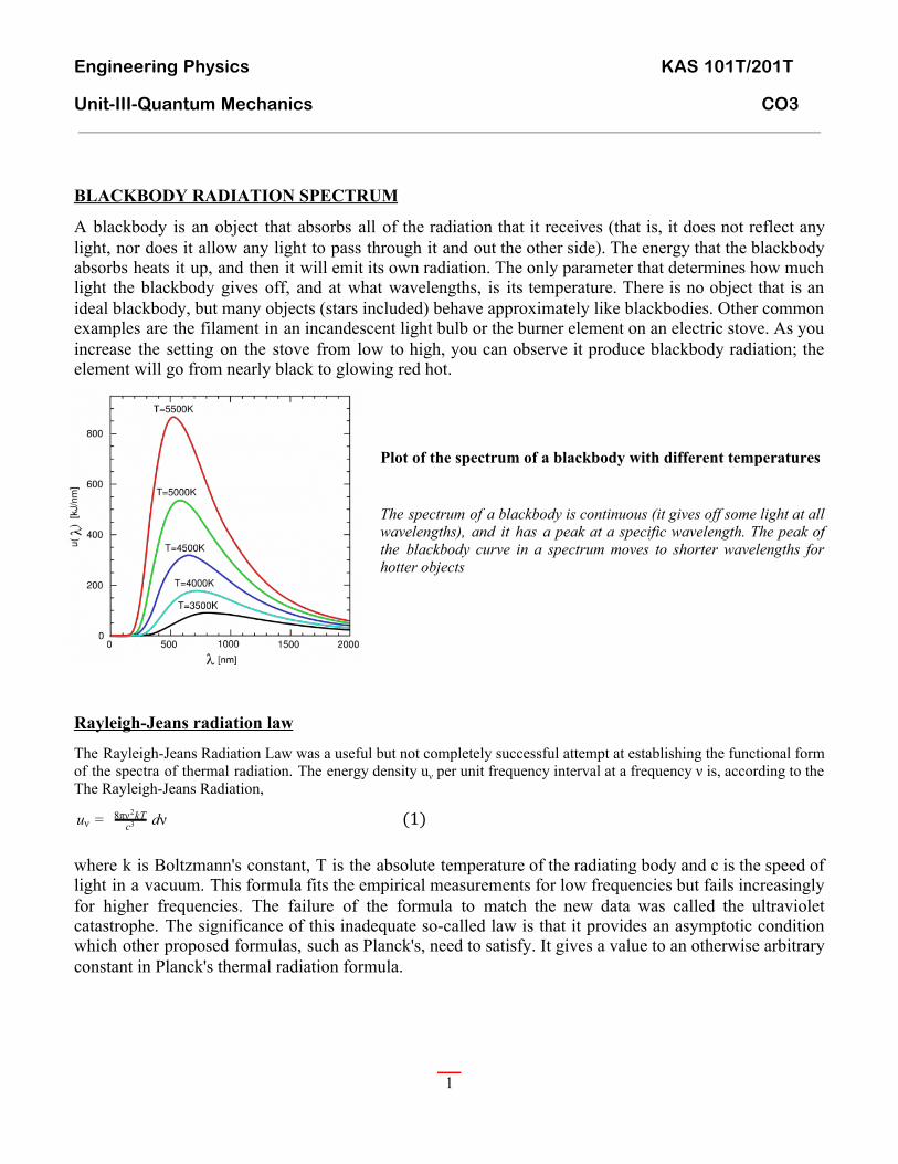
A blackbody is an object that absorbs all of the radiation that it receives (that is it does not reflect any light nor does it allow any light to pass through it and out the other side) The energy that the blackbody absorbs heats it up and then it will emit its own radiation The only parameter that determines how much light the blackbody gives off and at what wavelengths is its temperature There is no object that is an ideal blackbody but many objects (stars included) behave approximately like blackbodies Other common examples are the filament in an incandescent light bulb or the burner element on an electric stove As you increase the setting on the stove from low to high you can observe it produce blackbody radiation the element will go from nearly black to glowing red hot
Plot of the spectrum of a blackbody with different temperatures
The spectrum of a blackbody is continuous (it gives off some light at all wavelengths) and it has a peak at a specific wavelength The peak of the blackbody curve in a spectrum moves to shorter wavelengths for hotter objects
Rayleigh-Jeans radiation law
The Rayleigh-Jeans Radiation Law was a useful but not completely successful attempt at establishing the functional form of the spectra of thermal radiation The energy density uν per unit frequency interval at a frequency ν is according to the The Rayleigh-Jeans Radiation
(1) dνuν = c38πν kT2
where k is Boltzmanns constant T is the absolute temperature of the radiating body and c is the speed of light in a vacuum This formula fits the empirical measurements for low frequencies but fails increasingly for higher frequencies The failure of the formula to match the new data was called the ultraviolet catastrophe The significance of this inadequate so-called law is that it provides an asymptotic condition which other proposed formulas such as Plancks need to satisfy It gives a value to an otherwise arbitrary constant in Plancks thermal radiation formula
1
user
Textbox
37
Engineering Physics KAS 101T201T
Unit-III-Quantum Mechanics CO3
Stefanrsquos Law
The spectrum of radiation emitted by a solid material is a continuous spectrum unlike the line spectrum emitted by the same material in gaseous form The peak frequency of the emitted spectrum increases with the temperature of the solid body as does the total power radiated
Definition According to the Stefan-Boltzmann law the total power radiated by an ideal emitter (perfect blackbody) is proportional to the fourth power of the absolute temperature
P = AσT4
Where P = total power radiated from the blackbody
A = surface area of the blackbody σ = Stefan-Boltzmann constant
T = Absolute temperature of the blackbody To generalize
P = 120692AσT4
Where 120692 is the emissivity And
120692 = 1 for black body 120692 lt 1 for grey bodies (not perfect blackbody
Wienrsquos Displacement Law
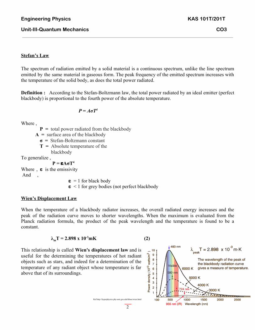
When the temperature of a blackbody radiator increases the overall radiated energy increases and the peak of the radiation curve moves to shorter wavelengths When the maximum is evaluated from the Planck radiation formula the product of the peak wavelength and the temperature is found to be a constant
λmT = 2898 x 10-3mK (2)
This relationship is called Wiens displacement law and is useful for the determining the temperatures of hot radiant objects such as stars and indeed for a determination of the temperature of any radiant object whose temperature is far above that of its surroundings
Refhttphyperphysicsphy-astrgsueduhbasewienhtml
2
user
Textbox
38
Engineering Physics KAS 101T201T
Unit-III-Quantum Mechanics CO3
Wienrsquos Distribution law
William Wien used thermodynamics to show that the spectral energy density of a blackbody between the wavelength range 120524 and 120524+d120524 is given by
E120582119889120582 = 119860 119891(120582119931) 119889120582 hellip (1)
1205825
Wien found using the Maxwell-Boltzmann distribution law for the speed of atoms (or molecules) in a gas that the form of the function f (120524T) was
119891(120582119931) = 119942 -120572 120582119931 hellip (2) And therefore
E120582119889120582 = 119860 120582-5 119942 -120572 120582119931119889120582 hellip (3) Where A and 120514 are constants to be determined Equation (3) is known as Wienrsquos Distribution Law Assumption of Quantum Theory of Radiation
The distribution of energy in the spectrum of radiations of a hot body cannot be explained by applying the classical concepts of physics Max Planck gave an explanation to this observation by his Quantum Theory of Radiation His theory says
a) The radiant energy is always in the form of tiny bundles of light called quanta ie the energy is absorbed or emitted discontinuously
b) Each quantum has some definite energy E=hν which depends upon the frequency (ν) of the radiations where h = Planckrsquos constant = 6626 x10-34Js
c) The energy emitted or absorbed by a body is always a whole multiple of a quantum ie nhνThis concept is known as quantization of energy
Planckrsquos Law(or Planckrsquos Radiation Law)
Plancks radiation law is derived by assuming that each radiation mode can be described by a quantized harmonic oscillator with energy En = nhν
Let N0 be the number of oscillators with zero energy ie E0 (in the so-called ground-state) then the numbers in the 1st 2nd 3rd etc levels (N1 N2 N3hellip) are given by
N exp N 1 = 0 ( kTminusE1 ) N exp N exp N 2 = 0 ( kT
minusE2 )N 3 = 0 ( kTminusE3 )
3
user
Textbox
39
Engineering Physics KAS 101T201T
Unit-III-Quantum Mechanics CO3
But since En = nhν
N exp N 1 = 0 ( kTminushν) N exp N exp N 2 = 0 ( kT
minus2hν) N 3 = 0 ( kTminus3hν)
The total number of oscillators N = N0 + N1 + N2 + N3helliphelliphelliphelliphellip
The total energy E = + + +hellipνN xp h 0 exp e ( kTminushν) exp 2hνN 0 ( kT
minus2hν) exp 3hνN 0 ( kTminus3hν)
The avg energy lt E gt = EN
lt E gt = N 1+exp xp ( ) +exp xp ( ) +hellip0[ e kTminushν e kT
minus2hν ]hνN exp xp ( ) + ( ) + ( ) +hellip0[ e kT
minushνkT
minus2hνkT
minus3hν ]
lt E gt = hν xp ( ) exp e kTminushν
1minusexp xp ( ) [ e kTminushν ]
(4)lt E gt = hν exp xp ( )minus1 [ e hν
kT ]
According to Rayleigh-Jeans law using classical physics the energy density uνper frequency interval was given by
(5)dνuν = c38πν kT 2
where kT was the energy of each mode of the electromagnetic radiation We need to replace the kT in this equation with the average energy for the harmonic oscillators that we have just derived above So we re-write the energy density as
(6)dνuν = c38πν2 hν
exp xp ( )minus1 [ e hνkT ]
Comparison of Rayleigh Jeans Wienrsquos amp Planckrsquos Radiation Laws for the blackbody radiation spectrum
4
user
Textbox
40
Engineering Physics KAS 101T201T
Unit-III-Quantum Mechanics CO3
WAVE PARTICLE DUALITY
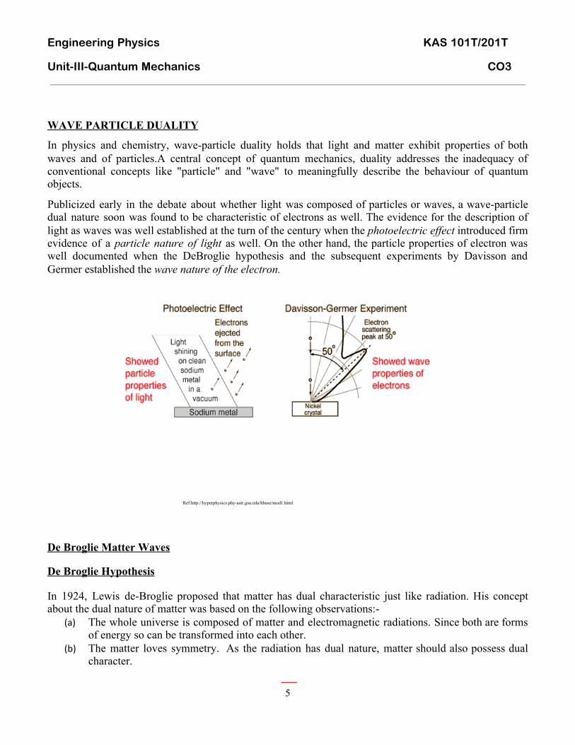
In physics and chemistry wave-particle duality holds that light and matter exhibit properties of both waves and of particlesA central concept of quantum mechanics duality addresses the inadequacy of conventional concepts like particle and wave to meaningfully describe the behaviour of quantum objects
Publicized early in the debate about whether light was composed of particles or waves a wave-particle dual nature soon was found to be characteristic of electrons as well The evidence for the description of light as waves was well established at the turn of the century when the photoelectric effect introduced firm evidence of a particle nature of light as well On the other hand the particle properties of electron was well documented when the DeBroglie hypothesis and the subsequent experiments by Davisson and Germer established the wave nature of the electron
Refhttphyperphysicsphy-astrgsueduhbasemod1html
De Broglie Matter Waves
De Broglie Hypothesis
In 1924 Lewis de-Broglie proposed that matter has dual characteristic just like radiation His concept about the dual nature of matter was based on the following observations-
(a) The whole universe is composed of matter and electromagnetic radiations Since both are forms of energy so can be transformed into each other
(b) The matter loves symmetry As the radiation has dual nature matter should also possess dual character
5
user
Textbox
41
Engineering Physics KAS 101T201T
Unit-III-Quantum Mechanics CO3
According to the de Broglie concept of matter waves the matter has dual nature It means when the matter is moving it shows the wave properties (like interference diffraction etc) are associated with it and when it is in the state of rest then it shows particle properties Thus the matter has dual nature The waves associated with moving particles are matter waves or de-Broglie waves
(7)λ = hmv
where λ = de Broglie wavelength associated with the particle h = Planckrsquos constant m = relativistic mass of the particle and v = velocity of the particle
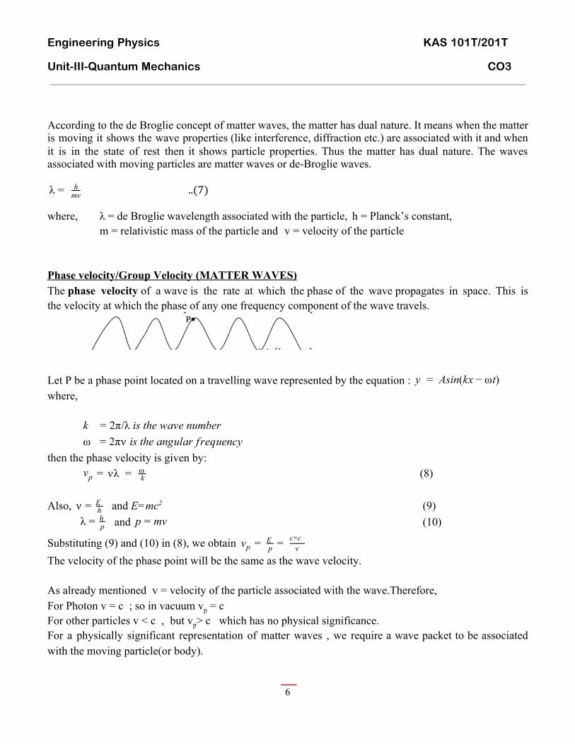
Phase velocityGroup Velocity (MATTER WAVES) The phase velocity of a wave is the rate at which the phase of the wave propagates in space This is the velocity at which the phase of any one frequency component of the wave travels Let P be a phase point located on a travelling wave represented by the equation Asin(kx t) y = minus ω where πλ is the wave number k = 2 ω πν is the angular f requency = 2
then the phase velocity is given by = vp λ ν = k
ω (8) Also and E=mc2ν = h
E (9) and λ = p
h v p = m (10)
Substituting (9) and (10) in (8) we obtain = = vp pE
vctimesc
The velocity of the phase point will be the same as the wave velocity As already mentioned v = velocity of the particle associated with the waveTherefore For Photon v = c so in vacuum vp = c For other particles v lt c but vpgt c which has no physical significance For a physically significant representation of matter waves we require a wave packet to be associated with the moving particle(or body)
6
user
Textbox
42
Engineering Physics KAS 101T201T
Unit-III-Quantum Mechanics CO3
The velocity of the wave packet is called Group Velocity 119907119892 = 119889120596 = 119889119864 (11)
119889119896 119889119901
BORN INTERPRETATION OF THE WAVE FUNCTION AND ITS SIGNIFICANCE Matter waves are represented by a complex function Ψ (xt) which is called a wave function The wave function is not directly associated with any physical quantity but the square of the wave function represents the probability density in a given region The wave function should satisfy the following conditions (i) Ψ should be finite (ii)Ψ should be single valued (iii) Ψ and its first derivative should be continuous (iv) Ψ should be normalizable
2 dV = 1 where V = volume in which the particle is expected to be foundint
VΨ| |
SCHRODINGERrsquoS WAVE EQUATION
TIME INDEPENDENT SCHRODINGERrsquoS EQUATION
The classical wave equation that describes any type of wave motion can be given as
= partx2part y(xt) 2 1
v2 partt2part y(xt)2
Where y is a variable quantity that propagates in lsquox lsquo direction with a velocity lsquovrsquo Matter waves should also satisfy a similar equation and we can write the equation for matter waves as
= (17)partx2part ψ(xt) 2 1
v2 partt2part ψ(xt)2
We can eliminate the time dependence from the above equation by assuming a suitable form of the wave function and making appropriate substitutions
7
user
Textbox
43
Engineering Physics KAS 101T201T
Unit-III-Quantum Mechanics CO3
(x ) ψ (x)e ψ t = 0minusiωt (18)
Differentiate eqn (18) wrt lsquoxrsquo successively to obtain
= (19)partx2part ψ(xt) 2
partx2part ψ (x) 2
0 eminusiωt
Differentiate eqn (18) wrt lsquotrsquo successively to obtain
= (20)partt2part ψ(xt) 2
minus ω) ψ (x)( i 20 eminusiωt
Substituting (19) and (20) in equation (17)
= = (21)partx2part ψ (x) 2
0 minus v2ω2 (x) ψ0 ψ (x) minus k2
0
= 0partx2part ψ (x) 2
0 ψ (x) + k20 (22)
Now we know the total energy lsquoE of the particle is the sum of its kinetic energy and potential energy
ie + V rArr (23)E = 2mp2
2m(E ) p2 = minus V
Also and rArr (24)k = λ2π λ = p
h k2 = h24π p2 2
Substituting (23) in (24) in then substituting result in (22) we get
= 0partx2part ψ (x) 2
0 ψ (x)+ h28mπ (EminusV )2
0 (25)
Replacing Ψ0(x )by Ψ (x) in eqn(vii) we obtain the Schrodingerrsquos time independent wave equation in one dimension as
= 0partx2part ψ(x) 2
ψ(x)+ h28mπ (EminusV )2
(26)
The above equation can be solved for different cases to obtain the allowed values of energy and the allowed wave functions
TIME DEPENDENT SCHRODINGERrsquoS EQUATION
In the discussion of the particle in an infinite potential well it was observed that the wave function of a particle of fixed energy E could most naturally be written as a linear combination of wave functions of the form
(x ) Ae ψ t = i(kxminusωt)
8
user
Textbox
44
Engineering Physics KAS 101T201T
Unit-III-Quantum Mechanics CO3
representing a wave travelling in the positive x direction and a corresponding wave travelling in the opposite direction so giving rise to a standing wave this being necessary in order to satisfy the boundary conditions This corresponds intuitively to our classical notion of a particle bouncing back and forth between the walls of the potential well which suggests that we adopt the wave function above as being the appropriate wave function for a free particle of momentum p = ℏk and energy E = ℏω With this in mind we can then note that
(27)partx2part ψ(x) 2
ψ(x) = minus k2
which can be written using = (28)E = p2
2m 2mℏ k2 2
From (28) and (27) we get
= (29) 2mminus ℏ 2
partx2 part ψ(x) 2
2m p ψ(x) 2
Similarly
= parttpartψ ωψ minus i (30)
which can be written using ω E = ℏ (31)
From (30) and (31)
= ℏ i parttpartψ ψ E (32)
We now generalize this to the situation in which there is both a kinetic energy and a potential energy present then E = p22m + V (x) so that
+ ψ E = 2mp ψ 2
(x)ψ V (33)
where Ψ is now the wave function of a particle moving in the presence of a potential V (x) But if we assume that the results above still apply in this case then we have by substituting (29) and (32) in (33)
+ 2mminus ℏ2
partx2 part ψ(x) 2
(x)ψ ℏ V = i parttpartψ (34)
which is the famous time dependent Schrodinger wave equation It is setting up and solving this equation then analyzing the physical contents of its solutions that form the basis of that branch of quantum mechanics known as wave mechanicsEven though this equation does not look like the familiar wave equation that describes for instance waves on a stretched string it is nevertheless referred to as a lsquowave equationrsquoas it can have solutions that represent waves propagating through space We have seen an example of this the harmonic wave function for a free particle of energy E and momentum p ieis a solution of this equation with as appropriate for a free particle V (x) = 0 But this equation can have distinctly non-wave like solutions whose form depends amongst other things on the nature of the potential V (x) experienced by the particle
9
user
Textbox
45
Engineering Physics KAS 101T201T
Unit-III-Quantum Mechanics CO3
(x ) Ae ψ t = i(pxminusEt)ℏ
In general the solutions to the time dependent Schrodinger equation will describe the dynamical behaviour of the particle in some sense similar to the way that Newtonrsquos equation F = ma describes the dynamics of a particle in classical physics However there is an important difference By solving Newtonrsquos equation we can determine the position of a particle as a function of time whereas by solving Schrodingerrsquos equation what we get is a wave function Ψ(x t) which tells us (after we square the wave function) how the probability of finding the particle in some region in space varies as a function of time
PARTICLE IN AN INFINITE POTENTIAL BOX
Consider a particle of mass lsquomrsquo confined to a one dimensional potential well of dimension lsquoLrsquo The potential energy V = infin at x=0 and x= L and V = 0 for 0le x le L The walls are perfectly rigid and the probability of finding the particle is zero at the wallsHence the boundary conditions are Ψ(x ) = 0 at x=0 and x= L The one dimensional time independent wave equation is
ψ(x) 0partx2part ψ(x) 2
+ℏ2
2m(EminusV ) = (35)
We can substitute V=0 since the particle is free to move inside the potential well
ψ(x) 0partx 2part ψ(x) 2
+ℏ2
2mE = (36)
Let and the wave equation (36) can be written isℏ2
2mE
= k2
ψ(x) 0 partx2part ψ(x) 2
+ k2 =
The above equation represents simple harmonic motion and the general solution is
(x) A sin kx B cos kx ψ = +
Applying the condition we get rArr B=0(x) at x ψ = 0 = 0 0 B 0 = A +
Applying the condition we get rArr k=(n120587) L(x) at x ψ = 0 = L sin kL 0 = A
where n = 0123hellip positive integer
Eigen values of energy
= = En = 2mk ℏ 2 2 n π h2 2 2
8π mL2 2n h2 2
8mL2 (37)
10
user
Textbox
46
Engineering Physics KAS 101T201T
Unit-III-Quantum Mechanics CO3
lsquonrsquo is the quantum number corresponding to a given energy level n=1 corresponds to the ground state n=2 corresponds to the first excited state and so on
Eigen functions
The allowed wavefunctions are
(x) ψn = A in (nπxL) s (38)
The constant A can be evaluated from normalization condition
sin (nπxL) intx=L
x=0A2 2 = 1
A = radic2L (39)
hence the eigen functions from(38) and (39) are
(x) ψn = radic2L in (nπxL) s (40)
Graphical representation of En Pn(x) and Ψn(x)for n = 12 and 3 quantum states
11
user
Textbox
47
Engineering Physics KAS 101T201T
Unit-III-Quantum Mechanics CO3
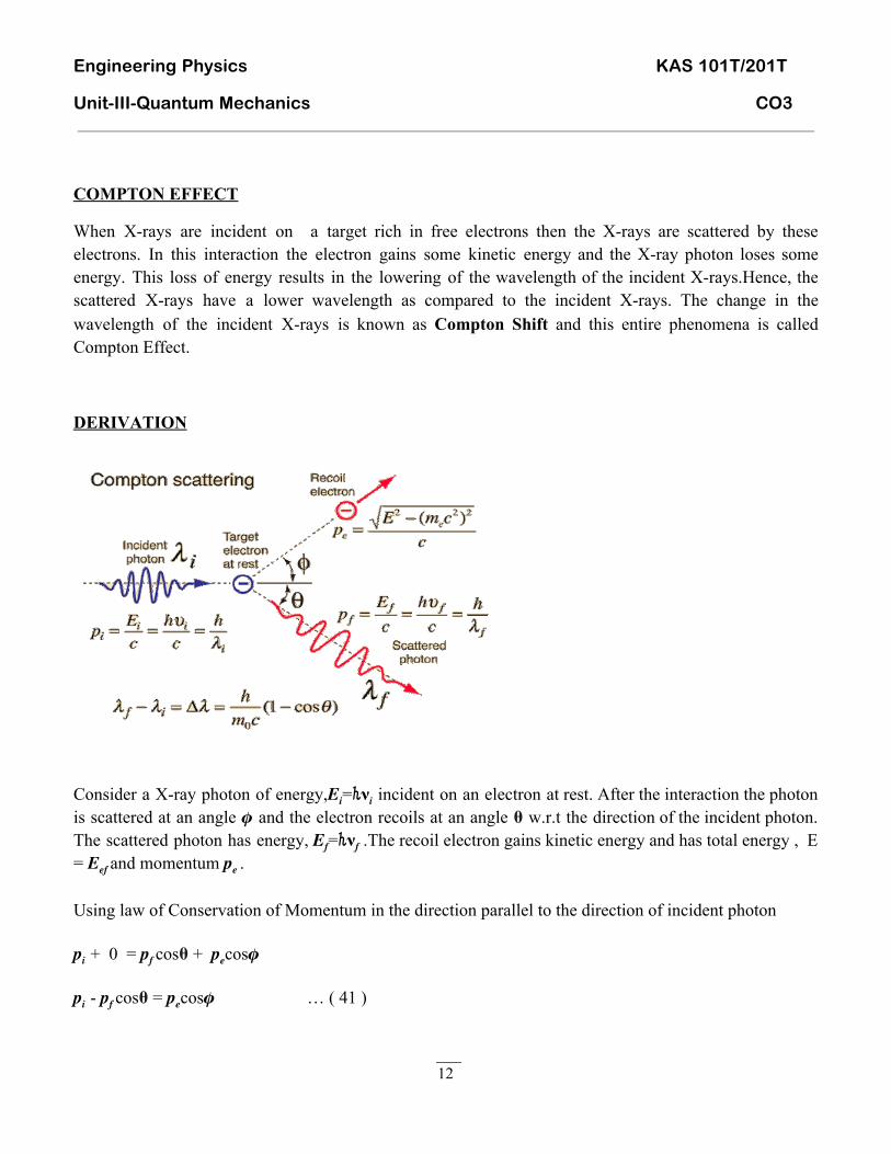
COMPTON EFFECT
When X-rays are incident on a target rich in free electrons then the X-rays are scattered by these electrons In this interaction the electron gains some kinetic energy and the X-ray photon loses some energy This loss of energy results in the lowering of the wavelength of the incident X-raysHence the scattered X-rays have a lower wavelength as compared to the incident X-rays The change in the wavelength of the incident X-rays is known as Compton Shift and this entire phenomena is called Compton Effect
DERIVATION
Consider a X-ray photon of energy119916 119946=ℎ120526119946 incident on an electron at rest After the interaction the photon is scattered at an angle 120659 and the electron recoils at an angle 120521 wrt the direction of the incident photon The scattered photon has energy 119916 119943=ℎ120526119943 The recoil electron gains kinetic energy and has total energy E = 119916 119942119943 and momentum 119953119942
Using law of Conservation of Momentum in the direction parallel to the direction of incident photon
119953 119946 + 0 = 119953 119943 cos120521 + 119953119942cos120659
119953 119946 - 119953 119943 cos120521 = 119953 119942cos120659 hellip ( 41 )
12
user
Textbox
48
Engineering Physics KAS 101T201T
Unit-III-Quantum Mechanics CO3
Using law of Conservation of Momentum in the direction perpendicular to the direction of incident photon
0 + 0 = 119953 119943 sin120521 - 119953 119942sin120659
119953 119943 sin120521 = 119953 119942sin120659 hellip ( 42 )
Squaring and adding eq( 41 ) and ( 42 ) we get
119953 119946 2 + 119953 1199432 cos2120521 - 2119953119946 119953119943 cos120521 + 119953 1199432 sin2120521 = 119953 1199422 (cos2120659 + sin2120659) hellip( 43 )
Simplifying eq(43) we get
119953 119946 2 + 119953 1199432 - 2119953 119946 119953 119943 cos120521 = 119953 1199422 hellip( 44 )
Using law of Conservation of Energy
119916 119946 + 119916 119942119946 =119916 119943 + 119916 119942119943
ℎ120526 119946 + 119950 0119940 2 = ℎ120526 119943 + 119916 119942119943 hellip( 45 )
Rearranging and squaring eq (45) we get
(ℎ120526 119946- ℎ120526 119943)2 + 119950 02119940 4 + 2(ℎ120526 119946-ℎ120526 119943)119950 01199402 = 119916 1199421199432 hellip( 46 )
We know that
119916 1199421199432 = 119953 1199422 119940 2 + 119950 02119940 4 hellip(47 )
Putting (47) in (46) we get
(ℎ120526 119946- ℎ120526 119943)2 + 119950 02119940 4 + 2(ℎ120526 119946-ℎ120526 119943)119950 01199402 = 1199531199422 1199402 + 119950 02119940 4
(ℎ120526 119946)2+ (ℎ120526 119943)2 - 2ℎ120526 119946ℎ120526 119943 + 2(ℎ120526 119946-ℎ120526119943)119950 01199402 = 119953 1199422 119940 2 hellip( 47a )
Putting (44) in (47a) (ℎ120526 119946)2+ (ℎ120526 119943)2 - 2ℎ120526 119946ℎ120526 119943 + 2(ℎ120526 119946-ℎ120526119943)119950 01199402 = ( 119953 1199462 + 1199531199432 - 2119953119946 119953119943 cos120521 )119940 2 hellip( 48 )
13
user
Textbox
49
Engineering Physics KAS 101T201T
Unit-III-Quantum Mechanics CO3
We know that
120526 119946 = 119940 120526 119943 = 119940 119953 119946 = ℎ 119953119943 = ℎ hellip( 49 )
120524 119946 120524 119943 120524119946 120524119943 Putting the eq(49) in eq(48 )
(ℎ119940)2 + (ℎ119940)2 - 2ℎ119940ℎ119940 + 2 (ℎ119940 - ℎ119940)119950 01199402 = (ℎ119940)2 + (ℎ119940)2 - 2ℎℎ cos120521 1199402
(120524 119946)2 (120524 119943)2 120524 119946120524 119943 120524 119946 120524119943 (120524119946)2 (120524119943)2 120524119946120524119943
-2ℎ119940ℎ119940 + 2ℎ119940(1 -1) 119950 01199402 = -119940 2 2ℎℎ cos120521 120524 119946 120524 119943 120524 119946 120524 119943 120524119946 120524119943 - ℎ + 119940(1 -1) 119950 0 = - ℎ cos120521
120524 119946120524 119943 120524 119946 120524 119943 120524 119946 120524119943
ℎ ( 1 - cos120521 ) = 119940 (1 -1) 119950 0
120524 119946120524 119943 120524 119946 120524119943
ℎ ( 1 - cos120521 ) = 119940 (120524119943 - 120524119946) 119950 0
120524 119946120524 119943 120524 119946120524119943
120524 119943 - 120524 119946 = ℎ ( 1 - cos120521 ) (50) 119950 0119940 Compton Shift ie Change in wavelength ∆120524 = 120524119943 - 120524119946 = ℎ ( 1 - cos120521 ) 119950 0119940 Maximum Compton Shift In eq(50) if 120521 = 180o then
∆120524 = ℎ ( 1 - (-1)) ) = 2ℎ = 2x663x10-34 = 00485Å (51) 119950 0119940 119950 0119940 91x10-31x3x108
14
user
Textbox
50
Engineering Physics KAS 101T201T
Unit-III-Quantum Mechanics CO3
Presence of Unmodified Radiation at non-zero scattering angles At times it happens that the X-ray photon interacts with bound electrons rather than with loosely held outer shell electrons In this case the photon does not have enough energy to knock out the tightly bound electron therefore the whole atom absorbs the energy transferred by the photon and then re-emits a photon of the same energy but in a different direction Hence we see a scattered photon having the same energy as that of the incident photon but travelling in a different direction Mathematically this means that in the equation for Compton Shift the mass of the electron m0 should be replaced by the mass of the atom M0 ie ∆120524 = 120524 119943 - 120524 119946 = ℎ ( 1 - cos120521 ) (52) M0119940 For example in case of Aluminium whose mass number is 27 M0 = 27x1836xm0 Maximum compton shift will be ∆120524 = 2ℎ = 00485Å = 98 x 10-17m which is negligible 27x1836xm0119940 27x1836 Kinetic Energy of recoil electron
The amount of energy lost by the photon equals the kinetic energy gained by the electron
KE of recoil electron = ℎ120526119946 - ℎ120526119943 (53)
KE of recoil electron = ℎc - ℎc 120524119946 120524119943
= ℎc( 120524 119943 - 120524 119946) 120524119943120524 i From (50)
= ℎc ℎ( 1 - cos120521) 119950 0119940 120524 119943120524i
15
user
Textbox
51
Engineering Physics KAS 101T201T
Unit-III-Quantum Mechanics CO3
= ℎ2( 1 - cos120521) (54) 119950 0120524 119943120524 i
Absence of Compton Scattering in the visible range of electromagnetic radiation The wavelength of visible light lies between 3800 Å - 7400 Å and the maximum compton shift is 00485Å Therefore as compared to the visible range this shift is negligible Hence if visible light is scattered from an electron-rich target the wavelength of the scattered light is the same as that of the incident For Your Information If a photon of wavelength 3800Å is scattered by a free election then a maximum compton shift of 00485Å can occur If we calculate then we see that 00485Å is just 0001 of 3800Å and such a small change can be neglected Whereas in the case of X-rays whose range lies between (01 Å - 10 Å) a change of 00485 Å is significant For example 00485 is 485 of 01Å and 0485 of 10Å and hence will be prominently observed
16
user
Textbox
52
Engineering Physics KAS 101T201T
Module-4-Wave Optics CO4
53
INTERFERENCE
41 Coherent Sources
It is found that it is not possible to show interference due to two independent sources of light because a
large number of difficulties are involved Two sources may emit light wave of different amplitude and
wavelength and the phase difference between the two may change with time The fundamental
requirement to get will defined interference pattern is that the phase difference between the two waves
should be constant The two sources are said to be coherent if they emit light waves of same
frequency nearly the same amplitude and are always in phase with each other
There are two type of coherence
1 Temporal coherence (Coherence in time) Longitudinal coherence is also known as temporal
coherence It is a measure of phase relation of a wave reaching at given points at two different
times Example- In Michelson-Morley experiment waves reaching at a given point at the same
time
2 Spatial coherence (Coherence in space) Transverse coherence or lateral coherence is also known
as spatial coherence It is a measure of phase relation between the waves reaching at two different
points in space at same time Example- In Young double slit experiment waves reaching at two
different points in space at the same time
In actual practice it is not possible to have two independent sources which are coherent But for
experimental purpose two virtual sources formed from a single source can act as coherent sources
A coherent source forms sustained interference patterns when superimposition of waves occur and the
positions of maxima and minima are fixed
Methods for producing interference pattern It is divided in following two classes for obtaining
interference
Division of wave front interference of light take place between waves from two sources formed due to
single source Example ndash interference by Young double slit
Division of amplitude interference takes place between the waves from the real source and virtual
source Example ndash interference by thin film
42 Interference in thin film An optical medium of thickness in the range of 05 to 10 may be considered as thin film
Interference can take place in a thin film by
i) Interference due to reflected light
ii) Interference due to transmitted light
Engineering Physics KAS 101T201T
Module-4-Wave Optics CO4
54
43 Interference in a Thin Film Due to Reflected Light Consider a ray SA of monochromatic light of wavelength λ be incident on the upper surface of a thin
transparent film of uniform thickness t as shown in the fig The ray SA is partly reflected along AB and
partly refracted along AC at an angle r The refracted ray AC is reflected from point C on the lower
surface of the film along CD and finally emerges out along DE To evaluate the path difference between
AB amp DE draw perpendiculars DL amp CN on AB amp DE respectively As the paths of the rays AB amp DE
beyond DL are equal so the optical path difference between these two rays is given by
Δ= micro(AC+CD)-AL -------------- (1)
In right angled triangle CNA we have
= cos r or
Ac =
=
-------------- (2)
angACN =r and CN =t
similarly in another right-angled triangle CND
we have
= cos r or CD =
=
-- --(3)
where angNCD =r
In right angled triangle ADL sin i =
or AL = AD Sin i = (AN+ND)Sin i ------- (4)
Again in triangles CNA amp CND
= tan r and
= tan r
AN = NC tan r and ND= NC tan r
AN = t tanr and ND = t tan r
From equation (4) AL= 2t tan r (Sin i)
AL = 2t tan r (micro Sin r ) [from Snellrsquos Law]
AL = 2 microt
------------ (5)
Substituting the values in equation (1)
Δ= micro (
+
) - 2 microt
Hence Δ= 2 micro t Cos r -------------------- (6)
As the ray AB is reflected from the denser medium therefore there occurs an additional path difference of
λ2 or a phase change of π between AB and DE
Total Path difference Δ= 2 micro t Cos r - λ2 ------------------- (7)
Engineering Physics KAS 101T201T
Module-4-Wave Optics CO4
55
This is the actual path difference produced between interfering reflected rays AB and DE
Condition for constructive interference and destructive interference
Constructive interference (Condition of Maxima )
In the case of maxima the path difference will be even multiple of λ2 ie
2 microt cos r- λ 2) =2 n( λ2)
2 microt cos r- λ 2) = n λ
2 microt cos r = (2n + 1) λ 2 where n= 0 1 2hellip
This is the condition for constructive interference and the film will appear bright
Destructive interference (Condition of Minima )
In the case of maxima the path difference will be odd multiple of λ2 ie
2 microt cos r- λ 2 = (2n + 1) λ 2
2 microt cos r = n λ n= 12 3helliphellip
This is the condition for destructive interference and the film will appear dark
44 Interference in a Thin Film Due to Transmitted Light Let a ray of light of wavelength λ be incident on the upper surface of a thin transparent film of uniform
thickness t and refractive index micro at an angle i as shown in fig The ray SA is refracted along AB at an
angle r The refracted part AB is partly reflected along BC and partly refracted along BP at an angle i The
reflected part BC is again reflected from point C on the upper surface of the film along CD and finally
emerges out along DQ which are derived from the same incident ray and hence are coherent To evaluate
the path difference between BP amp DQ the
perpendiculars DN amp CM are drawn on BP amp BD
respectively
Δ= micro(BC+CD) - BN --- (1)
In right angled triangle CBM we have
= cos r or
BC =
=
----(2)
angBCM =r and MC =t
similarly in another right-angled triangle MDC
Engineering Physics KAS 101T201T
Module-4-Wave Optics CO4
56
we have
= cos r or CD =
=
-- --(3) where angMCD =r
In right angled triangle BND sin i =
or BN = BD Sin i = (BM+MD) Sin i ---- (4)
Again in triangles BMC amp CDM
= tan r and
= tan r
BM = CM tan r and MD= CM tan r
BM = t tan r and MD = t tan r
From equation (4) BN= 2t tan r (Sin i)
BN = 2t tan r (micro Sin r) [from Snellrsquos Law]
BN = 2 microt
---- (5)
Substituting the values in equation (1)
Δ= micro (
+
) - 2 microt
Δ= 2 micro t Cos r ------ (6)
This is the path difference produced between interfering refracted rays BP and DQ
Condition for constructive interference and destructive interference
Constructive interference (Condition of Maxima )
In the case of maxima the path difference will be even multiple of λ2 ie
2 microt cos r =2 n( λ2)
2 microt cos r = n λ where n= 0 1 2hellip
This is the condition for constructive interference and the film will appear bright
Destructive interference (Condition of Minima )
In the case of maxima the path difference will be odd multiple of λ2 ie
2 microt cos r = (2n + 1) λ 2
2 microt cos r = (2n + 1) λ 2 n= 12 3helliphellip
This is the condition for destructive interference and the film will appear dark Hence the conditions of
maxima and minima in transmitted light are just opposite to the reflected light
Engineering Physics KAS 101T201T
Module-4-Wave Optics CO4
57
Colours of thin films When white light is incident on a thin film only few wavelengths will satisfy
the condition of maxima and therefore corresponding colours will seen in the pattern For other
wavelengths condition of minima is satisfied and so corresponding colours will be missing in the pattern
The coloration of film varies with t and r Therefore if one varies either t or r a different set of colours
will be observed Since the condition for maxima and minima are opposite in case of reflected and
transmitted pattern So the colours found in two patterns will be complimentary to each other
45 Necessity of broad source or extended Source When point source is used only a small
portion of the film can be seen through eye and as a result the whole interference pattern cannot be seen
But when a broad source is used rays of light are incident at different angles and reflected parallel beam
reach the eye and whole beam and complete pattern is
visible
46 Interference Due to non-uniform Thin film (Wedge shaped thin film)
The wedge-shaped film as shown in Figure 45 Let a ray
from S is falling on the film and after deflections produce
interference pattern The path difference between PQ and EH
∆= [(PF + FE)film - (PK)air]
= micro (PF + FE) ndash (PK)
= micro (PN + NF + FE) ndash PK
= micro (PN + NF + FE ndash PN)
= micro (NF +FE)
∆ = micro (NF + FL)
∆ = micro (NL)
In Triangle ENL
= Cos(r+Ɵ)
NL = EL Cos(r+Ɵ) = 2t Cos(r+Ɵ)
Therefore ∆ = 2 micro t cos (r +θ)
Then total path difference considering refraction from denser medium is taking place
∆ = 2 microt cos (r+θ) ndash λ2
In triangle PKE 119878119894119899 119894 =119875119870
119875119864
In triangle PNE 119878119894119899 119903 =119875119873
119875119864
119878119894119899 119894
119878119894119899 119903 = micro
119875119870
119875119864119875119864
119875119873 = micro then PK = microPN
In triangles EFR amp FRL FR is common ER= RL=t
angFER=angFLR =r+Ɵ
So both are congruent triangles therefore EF=FL
Engineering Physics KAS 101T201T
Module-4-Wave Optics CO4
58
Condition for maxima
2microcos (r + θ) = (2n + 1) λ2 where n = 0 1 2 hellip
This is the condition for constructive interference and the film will appear bright
Condition for minima
2microcos (r + θ) = nλ where n = 0 1 2 hellip
This is the condition for destructive interference and the film will appear dark
47 Newtonrsquos Ring Experiment
Newtonrsquos rings It is a special case of interference in a film of variable thickness such as that formed
between a plane glass plate and a convex lens in contact with it When monochromatic light falls over it
normally we get a central dark spot surrounded by alternatively bright and dark circular rings When
white light is used the rings would be coloured
Experimental Arrangement Let S be the extended
source of light rays from which after passing through a
lens L falls upon a glass plate Gat 45deg After partial
reflection these rays fall on a plano convex lens P placed
on the glass plate E The interference occurs between the
rays reflected from the two surfaces of the air film and
viewed through microscope M as shown Figure
Theory The air film formed is of wedge shape so the
path difference produced will be
∆= 2 microt cos (r+θ) ndash λ2
For normal incident r = 0 and θ is very small because of large radius of curvature So neglecting r and θ
the path difference will be
So ∆= 2 microt-λ2
At the point of contact t = 0
So ∆=λ2 The central fringe will be dark
Condition for maxima
2 microt = (2n + 1) λ2 where n = 0 1 2
Engineering Physics KAS 101T201T
Module-4-Wave Optics CO4
59
This is the condition for constructive interference and the film will appear bright
Condition for minima
2 microt = nλ where n = 0 1 2
This is the condition for constructive interference and the film will appear bright we get alternatively
bright and dark rings
Diameter of the rings
NP x NQ = ND x NO
NP= NQ= r radius of ring under consideration
NO =t ND= OD-ON OD= 2R
Then r2= t (2R- t) = 2Rt- t
2 = 2Rt
t = r22R
Diameter of bright rings From the condition of maxima put the
value of t we get
=
( )
r2
n = ( )
= (
)
Dn2
= ( )
Dn2 =
2(2n + 1) λR (For air micro = 1)
Dn =radic(2λR) radic(2n + 1)
Dn radic( + )
Thus the diameter of bright rings are proportional to the square root of the odd natural numbers
Diameter of dark ring Using the condition for minimum and put the value of t
= nλ
Engineering Physics KAS 101T201T
Module-4-Wave Optics CO4
60
which gives
(Dn)2 = 4nλR
Or Dn = radic R
Dn radic
Thus the diameter of dark rings are proportional to the square root of natural numbers
48 Application of Newtonrsquos Ring
481 Measurement of Wavelength of sodium light by Newtonrsquos Rings
For dark rings we know that
=
To avoid any mistake one can consider two clear fringes nth
and (n + p)th
So (Dn)2 = 4nλR --------(1)
(Dn+p)2 = 4(n+p) λR ------(2)
Subtracting these two equation we get ((Dn+p)2 - (Dn)
2) = 4p λR
Or λ =( )
( )
Wavelength can be calculated if you know diameters of the rings order of the ring and radius of curvature
(R)
482 Measurement of Refractive Index of Liquid by Newtonrsquos Rings
For this purpose liquid film is formed between the lens and glass plate
For dark rings we know that =
To avoid any mistake one can consider two clear fringes nth
and (n + p)th
So (Dn)2 =
and (Dn+p)
2 =
( )
Engineering Physics KAS 101T201T
Module-4-Wave Optics CO4
61
Subtracting these two we get [(Dn+p)2 - (Dn)
2)]liquid =
-----(1)
For air micro=1 equation (1) can be written as [(Dn+p)2 - (Dn)
2)]air = 4pλR -----(2)
Divide equation (2) by equation (1)
= ( )
( )
( ) ( )
One can see that rings contract with the introduction of liquid
Engineering Physics KAS 101T201T
Module-4-Wave Optics CO4
62
DIFFRACTION
The phenomenon of bending of light round the corners of an obstacle and their spreading into the
geometrical shadow (of an object) is called diffraction and the distribution of light intensity resulting in
dark and bright fringes (that is with alternate maxima and minima) is called a diffraction pattern
This phenomenon was first discovered in 1665 by an Italian scientist named Grimaldi and was studied by
Newton Fresnel was able to explain successfully the phenomenon of diffraction by considering that the
diffraction phenomenon is caused by the interference of innumerable secondary wavelets produced by the
unobstructed portions of the same wave front
The diffraction phenomenon is usually divided into two categories
(i) Fresnelrsquos diffraction In this class either the source of light or screen or both are in general at a finite
distance from the diffracting element but no lenses are needed for rendering the rays parallel or
convergent Therefore the incident wave front is either spherical or cylindrical instead of being plane
(ii) Fraunhoferrsquos diffraction In this class both the source and the screen are effectively at infinite
distance from the diffracting element It is observed by employing two convergent lenses one to render
the incoming light parallel and the other to focus the parallel diffracted rays on the screen Therefore the
incident wave front is plane
49 Fraunhofer diffraction at a single Slit
Let S is a source of monochromatic light of wavelength lsquoλrsquo L is collimating lens AB is a slit of width a
Lrsquo is another converging lens and XY is the screen light coming out from source and passing through slit
is focused at the screen A diffraction pattern is obtained on the screen which consists of central bright
band having alternate dark and bright bands of decreasing intensity on both the sides The complete
arrangement is shown in Figure
Analysis and Explanation According to
Huygenrsquos theory a point in AB send out secondary
waves in all directions The diffracted ray along
the direction of incident ray is focussed at C and
those at an angle θ are focused at P and Prsquo Being
at equidistant from all slits points secondary wave
will reach in same phase at point C and so the
intensity will be maximum there For the intensity
at P let AN is normal to BN then path difference
between the rays emanating from extreme points
A and B of the slit AB is given by
Engineering Physics KAS 101T201T
Module-4-Wave Optics CO4
63
∆ = BN = AN sin θ = a sin θ
Corresponding phase difference is
sin
2a
which is zero for the ray from A and maximum for the ray from B Let AB consists of n secondary
sources then the phase difference between any two consecutive source will be
sin
21a
n = δ (say)
According to the theory of composition of n simple harmonic motions of equal amplitude (a) and
common phase difference between successive vibrations the resultant amplitude at P is given by
na
a
a
n
aRsinsin
sinsin
2sin
2sin
)1(sin
sin
sin
sin
sin
AR
naR
n
a
n
aR
The resultant intensity at P which is the square of the resultant amplitude R is given by
I = R2 = A
2 sin
2 α α
2 (2)
Condition of Maxima and Minima
Principal Maximum(central maxima)
The resultant amplitude given by equation (1) can be expanded as
1206
sin 53
AAR
Where α = πa sinθ λ
Where A= nα
Engineering Physics KAS 101T201T
Module-4-Wave Optics CO4
64
R will be maximum if the negative term vanish This is possible only when α= πa sinθ λ =0 or θ=0 Thus
the maximum value of resultant amplitude R at C is A and the corresponding maximum intensity is
proportional to 2A
Positions of Minima
From equation (2) it is clear that the intensity is minimum when sinα=0
Then
na
na
n
sin
sin
32
Where n=123 gives the directions of first second third minima
Secondary Maxima
from equation (2) secondary maxima will be
= 0 =gt
[A
2 sin
2 α α
2] = 0
A2
( )
ie either ( )
the equation gives the value of (except ) for which the
intensity is zero on the screen Hence position of secondary maxima are given by the roots of the equation
The value of satisfying the above equation are obtained
graphically by plotting the curves
The point of intersection of two curves give the value of
which satisfy the above equation
The point of intersection will give
α = 0 plusmn 3π2 plusmn 5 π 2 plusmn 7 π 2
Engineering Physics KAS 101T201T
Module-4-Wave Optics CO4
65
=0 plusmn 143 π plusmn 2462 π plusmn 3471 π
The first value α = 0 correspond point to central maximum The remaining value of α gives secondary
maxima
α = plusmn 3π2 plusmn 5 π 2 plusmn 7 π 2hellip
α = ( )
where n= 1 23hellip
Intensity Distribution
a) Intensity of Central Maxima at α = 0
I= Lt A2 [ sin
2 α α
2 ]= A
2 = I0
b) Intensity of First Secondary Maxima for first(n=1) secondary maxima α = 3π2 Then equation
(2) will be
I1 = A 2 (sin 3π2)
2(3π2)
2= 4 I0 9π
2 = I0 22
c) Intensity of second Secondary Maxima for second(n=1) secondary maxima α = 5π2 Then
equation (2) will be
I2 = A 2 (sin 5π2)
2(5π2)
2= 4 I0 25π
2 = I0 62
The diffraction pattern consists of a bright central maximum surrounded by minima and the intensity of
secondary maxima goes on decreasing very rapidly
410 Fraunhoferrsquos diffraction at a double slit
Let us suppose two parallel slits AB and DE each of width lsquoarsquo and separated by opaque distance lsquobrsquo Let a
plane wave front of monochromatic light of wavelength λ be incident normally upon the slits Suppose the
light diffracted by the slits be focused by a convex lens L on the screen XY situated in the focal plane of
the lens The diffraction pattern obtained on the screen is characterized by a number of equally spaced
interference maxima and minima in the region normally occupied by the central maximum in the single
slit diffraction
Engineering Physics KAS 101T201T
Module-4-Wave Optics CO4
66
Explanation According to the theory of diffraction at a single slit the resultant amplitude due to all the
wavelets from each slit is given by
sinAR (1)
where α = πa sinθ λ (2)
We can replace all secondary waves from the slit AB by a
single wave of amplitude R and phase α originating from its
middle point S1 Similarly all the secondary wavelets in the
second slit DE can also be replaced by the similar wave originating from its middle point S2 Hence the
resultant amplitude at a point P on the screen will be due to
the interference between the two waves of same amplitude
R and a phase difference φ originating from S1 and S2
Let us drop a perpendicular S1M on S2M The path
difference between the two wave originating from S1 and
S2 and reaching at P after travelling in the direction θ will
be
S2M= (a+b) sin θ (3)
Therefore the corresponding phase difference between
them is
sin
2ba (4)
The resultant amplitude at P can be obtained by the vector amplitude diagram QR and RS represent the
amplitude of the two waves originating from S1 and S2 and angle φ as phase difference between them
2cos4
)cos1(2
cos2
cos))((2
22
2
222
222
R
R
RRRRR
RSQRRSQRQS
(5)
Substituting the values of R and φ from equations (1) and (4) in equation (5) we get
Engineering Physics KAS 101T201T
Module-4-Wave Optics CO4
67
)7(sin)2
)6(cossin
4 2
2
222
ba
AR
Therefore the resultant intensity at P is
2
2
222 cos
sin4ARI (8)
This is the required expression for the intensity distribution due to a Fraunhoferrsquos diffraction at a double
slit
It is clear from equation (8) that the resultant intensity at any point on the screen depends on two factors
1 2
2sin
which gives diffraction pattern due to each single slit
2 2cos which gives the interference pattern due to two waves of same amplitude (R) originating
from the mid-points of their respective slits
Hence the resultant intensity due to double slit of equal width at any point on the screen is given by
the product of 2
2sin
and 2cos If either of these factor is zero the resultant intensity will also be
zero Let us now consider the effect of each factor
(i) Principal maxima is given by 2
22 sin
A θ=0
Position of minima are given by
Sinα=0 α is non-zero
m m=123
a
m
ma
sin
sin
m=123
Position of secondary maxima approach to
Engineering Physics KAS 101T201T
Module-4-Wave Optics CO4
68
2
7
2
5
2
3
(ii) According to interference term 2cos I is maximum when 2cos =1
n n=0123
nba
nba
sin
sin
n=0123
Intensity is minimum when 2cos =0 β=(2n+1)π2
sinba =(2n+1)π2
Thus the entire pattern due to double slit may be considered as consisting of interference fringes due
to light from both slits The intensities of these fringes being governed by diffraction occurring at the
individual slits
Engineering Physics KAS 101T201T
Module-4-Wave Optics CO4
69
411 Plane Transmission Diffraction Grating (N-Slits DiffractionDiffraction due
to double slits)
A plane diffraction grating is an arrangement consisting of a large number of close parallel straight
transparent and equidistant slits each of equal width a with neighbouring slits being separated by an
opaque region of width b A grating is made by drawing a series of very fine equidistant and parallel lines
on an optically plane glass plate by means of a fine diamond pen The light cannot pass through the lines
drawn by diamond while the spacing between the lines is transparent to the light There can be 15000
lines per inch or more is such a grating to produce a diffraction of visible light The spacing (a + b)
between adjacent slits is called the diffraction element or
grating element If the lines are drawn on a silvered surface of
the mirror (plane or concave) then light is reflected from the
positions of mirrors in between any two lines and it forms a
plane concave reflection grating Since the original gratings
are quite expensive for practical purposes their photographic
reproductions are generally used
The commercial gratings are produced by taking the
cast of an actual grating on a transparent film such as cellulose
acetate A thin layer of collodin solution (celluloid dissolved in a volatile solvent) is poured on the surface
of ruled grating and allowed to dry Thin colluding film is stripped off from grating surface This film
which retains the impressions of the original grating is preserved by mounting the film between two glass
sheets Now-a-days holographic gratings are also produced Holograpic gratings have a much large
number of lines per cm than a ruled grating Theory of Grating Suppose a plane diffraction grating
consisting of large number of N parallel slits each of width a and separation b is illuminated normally by
a plane wave front of monochromatic light of wavelength A as shown in Figure The light diffracted
through N slits is focused by a convex lens on screen XY placed in the focal plane of the lens L The
diffraction pattern obtained on the screen with very large number of slit consists of extremely sharp
principle interference maximum while the intensity of secondary maxima becomes negligibly small so
that these are not visible in the diffraction pattern Thus if we increase the number of slits (N) the
intensity of principal maxima increases
Explanation
According to Huygenrsquos principle all points within each slit become the source of secondary wavelets
which spread out in all directions From the theory of Fraunhofer diffraction at a single slit the resultant
amplitude R due to all waves diffracted from each slit in the direction θ is given by
sinAR where A
is a constant and α = πa sinθ λ Thus the resultant of all secondary waves may be treated as a single wave
of amplitude R and phase α starting from the middle point of each slit and travelling at an angle θ with
the normal Thus the waves diffracted from all the N slits in direction θ are equivalent to N parallel
waves each starting from the middle points S1 S2 S3 Sn-1 Sn of slits Draw perpendicular S1Kn-1 from
S1 on SnKn-1 then the path difference between the waves originating from the slits S1 and S2 is
Engineering Physics KAS 101T201T
Module-4-Wave Optics CO4
70
S2K1=S1S2 sin θ= (a+b) sin θ
Similarly between rays from S2 and S3 will be
S3K2=S2S3 sin θ=(a+b) sin θ
Thus the path difference between the waves from any two consecutive slits is (a+b) sin θ Therefore the
corresponding phase difference is 2πλ(a+b) sin θ=2β Therefore as we pass from one vibration to another
the path goes on increasing by an amount (a+b) sin θ and corresponding phase goes on increasing by an
amount 2πλ(a+b) sin θ Thus phase increases in arithmetical progression therefor the problem reduces to
find the resultant amplitude of N waves of equal amplitude
sinAR and period but the phase
increasing in AP In this case the resultant amplitude in the direction θ is given by
sin
sin
sin
sin
sin NA
NRR
The corresponding intensity at P is given by
2
2
2
222
sin
sin
sin NARI (1)
The first factor of equation (1) that is 2
22 sin
A represents intensity distribution due to diffraction at a
single slit whereas the second factor That is
2
2
sin
sin N gives the distribution of intensity in the
diffraction pattern due to the interference in the waves from all the N slits
Principal maxima
The condition for principal maxima is
sin β = 0 ie β = plusmn nπ where n = 0 1 2 3 hellip middot
πλ (a + b) sin θ = plusmn nπ =gt (a + b) sin θ = plusmn n λ hellip (1)
If we put n = 0 in equation (1) we get θ = 0 and equation (1) gives the direction of zero
order principal maximum The first second third hellip order principal maxima may be obtained
by putting n = 1 2 3 in equation (1)
Minima The intensity is minimum when
Engineering Physics KAS 101T201T
Module-4-Wave Optics CO4
71
sin Nβ = 0 but sin β 0
Therefore Nβ = plusmn mπ
N πλ (a + b) sin θ = plusmn mπ
N (a + b) sin θ = plusmn mλ (2)
Here can have all integral values except 0 N 2N 3N hellip because for these values of m sin 13 = 0 which
gives the positions of principal maxima Positive and negative signs show that the minima lie
symmetrically on both sides of the central principal maximum It is clear from equation (2) that form= 0
we get zero order principal maximum m = 1 2 34 = (N -1) gives minima governed by equation (2) and
then at m = N we get principal maxima of first order This indicates that there are (N -1) equispaced
minima between zero and first orders maxima Thus there are (N ndash 1) minimum between two successive
principal maxima
Secondary Maxima The above study reveals that there are (N- 1) minima between two successive
principal maxima Hence there are (N -2) other maxima coming alternatively with the minima between
two successive principal maxima These maxima are called secondary maxima To find the positions of
the secondary maxima we first differentiate equation with respect to β and equating to zero
dIdβ = A 2
sin2 a a
2 2 [sin Nβsin β ] N cos Nβ sin β- sin N cos βsin 2β =0
N cos Nβ sin β = sin Nβ cos β = 0
tan Nβ N tan β
To find the intensity of secondary maximum we make
these of the triangle shown in Figure We have sin Nβ = N
tan βradic (1+N 2 tan
2 β)
Therefore sin 2β sin
2β =(n
2 tan
2β sin
2β (1+n
2 tan
2β )
sin 2Nβ sin
2β =(n
2 tan
2β(1+N tan
2) sin
2β
= N 2(1+n
2 sin
2β )
Putting this value of sin 2 Nβ sin
2 β we get
IS =A2 sin
2α α
2 =N
2[1+(N
2-1) SIN
2 β
This indicates the intensity of secondary maxima is
proportional to
N 2 [1+(N2-1) sin 2 β] whereas the intensity of principal maxima is proportional to N2
Engineering Physics KAS 101T201T
Module-4-Wave Optics CO4
72
412 Absent Spectra with a Diffraction Grating
It may be possible that while the first order spectra is clearly visible second order may be not be visible at
all and the third order may again be visible It happen when for again angle of diffraction 0 the path
difference between the diffracted ray from the two extreme ends of one slit is equal to an integral multiple
of A if the path difference between the secondary waves from the corresponding point in the two halves
will be A2 and they will can all one another effect resulting is zero intensity Thus the mining of single
slit pattern are obtained in the direction given by
a sin θ= mλ hellip(1 )
where m = 1 2 3 helliphellip excluding zero but the condition for nth order principles maximum in
the grating spectrum is (a + b) sin θ = nλ hellip (2)
If the two conditions given by equation (2) are simultaneously satisfied then the direction in which the
grating spectrum should give us a maximum every slit by itself will produce darkness in that direction and
hence the most favourable phase for reinforcement will not be able to produce an illumination ie the
resultant intensity will be zero and hence the absent spectrum Therefore dividing equation (2) by
equation (1)
(a+ b) sine θa sin θ =n m
(a+ b) a =nm
This is the condition for the absent spectra in the diffraction pattern
If a= b ie the width of transparent portion is equal to the width of opaque portion then
from equation (3) n = 2m ie 2nd 4th 6th etc orders of the spectra will be absent corresponds to the
minima due to single slit given by m = 1 2 3 etc
b = 2a amp n=3m
ie 3rd 6th 9th etc order of the spectra will be absent corresponding to a minima due to a
single slit given by m = 1 2 3 etc
413 Number of Orders of Spectra with a Grating
The number of spectra that are visible in a given grating can be easily calculated with the help
of the equation
Engineering Physics KAS 101T201T
Module-4-Wave Optics CO4
73
(a + b) sin θ = n λ
n=(a+b) sin θλ
Here (a+ b) is the grating element and is equal to 1N = 254 N cm N being number of lines per inch in
the grating Maximum possible value of the angle of diffraction e is 90deg Therefore sin θ = 1 and the
maximum possible order of spectra
N max=(a+b)λ
If (a + b) is between λ and 2 λ ie grating element (a + b) lt 2 λ then
n maxlt2 λ λ lt 2
and hence only the first order of spectrum is seen
414 Dispersive Power of a plane diffraction grating
The dispersive power of a diffraction grating is defined as the rate of change of the angle of diffraction
with the change in the wavelength of light used
Thus if the wavelength changes from λ to (λ+dλ) and corresponding angle of diffraction changes from θ
to (θ+dθ) then the ratio dθdλ is called the dispersive power of the grating
For plane diffraction grating we have the grating equation for normal incidence as
(a + b) sin θ = n λ (10
Where (a+b) is the grating element and θ the angle of diffraction for nth
order spectrum
Differentiating eqn (1) with respect to λ we get nd
dba
cos)(
Therefore the dispersive power
cosba
n
d
d
(2)
Engineering Physics KAS 101T201T
Module-4-Wave Optics CO4
74
2
2
21
21
1
1
sin1
n
bad
d
ba
nba
n
ba
n
d
d
In the above equation dθ is the angular separation between two spectral lines with difference in
wavelengths as dλ
415 Resolving Power of Optical Instruments
When two objects are very class to each other it may not be possible for our eye to see them separately If
we wish to see them separately then we will have to make use of some optical instruments like
microscope telescope grating prism etc The ability of an optical instrument to form distinctly separate
images of two objects very close to each other is called the resolving power of instrument A lens system
like microscope and telescope gives us a geometrical resolution while a grating or a prism gives a spectral
resolution In fact the image of a point object or line is not simply a point or line but what we get is a
diffraction pattern of decreasing intensity For a two point system two diffraction patterns are obtained
which may and may not overlap depending upon their separation The minimum separation between two
objects that can be resolved by an optical instrument is called resolving limit of that instrument The
resolving power is inversely proportional to the resolving limit
4151 Rayleigh Criterion of Resolution
According to Lord Rayleighrsquos arbitrary criterion two nearby images are said to be resolved if (i) the
position of central maximum of one coincides with the first minima of the other or vice versa
Engineering Physics KAS 101T201T
Module-4-Wave Optics CO4
75
To illustrate this let us consider the diffraction patterns due to two wavelengths λ1and λ 2 There may be
three possibilities First let the difference (λ1 -λ 2) is sufficiently large so that central maximum are quite
separate this situation is called well resolved Secondly consider that (λ) is such that central maximum
due to one falls on the first minima of the other The resultant intensity curve shows a distinct dip in the
middle of two central maxima This situation is called just resolved as the intensity of the dip can be
resolved by our eyes
ldip = 081 Imax hellip (1)
Thirdly let the (λ1-λ2) is very small such that they come still closes as shown in Figure The intensity
curves have sufficient overlapping and two images cannot be distinguished separately The resultant curve
almost appears as one maxima This case is known as unsolved Thus the minimum limit of resolution is
that when two patterns are just resolved
4152 Resolving Power of Plane Diffraction Grating
We know that the diffraction grating has ability to produce spectrum ie to separate the lines of nearly
equal wavelengths and therefore it has resolving capability The resolving power of a grating may be
defined as its ability to form separate diffraction maxima of two wavelengths which are very close to each
other If A is the mean value of the two wavelengths and dλ is the difference between two then resolving
power may be defined as resolving power = λ dλ
Expression for resolving power Let a beam of light having two wavelengths λ1 and λ2 is falling
normally on a grating AB which has (a + b) grating element and N number of slits as shown in Figuremiddot
After passing through grating rays forms the diffraction patterns which can be seen through telescope
Now if these patterns are very close together they overlap and cannot be seen separately However if
they satisfy the Rayleigh criterion that is the wavelengths can be just resolved when central maxima due
to one falls on the first minima of the other
Let the direction of nth principal maxima for wavelength
A1 is given by
(a + b) sin θn = nλl Or N (a + b) sin θn = Nnλ1
and the first minima will be in the direction given by
N (a+b)sin (θn +dθn) =mλ1
where m is an integer except 0 N 2N hellip because at
these values condition of maxima will be
satisfied The first minima adjacent to the nth maxima will be in the direction (θn +dθn ) only
when m = (nN + 1) Thus
Engineering Physics KAS 101T201T
Module-4-Wave Optics CO4
76
N (a + b) sin (θn + dθn) = (nN + 1) λ1
Therefore (a +b) sin (θn + dθn) = nλ2 or N (a + b) sin (θn + dθn) = Nnλ2
Now equating the two equations
(nN + 1) λ1 = Nn λ2 or (nN + 1) λ =Nn (λ + dλ)
λ = Nndλ
λ1 = λ λ2 -λ1 = dλ λ2 = λ + dλ
Thus resolving power of grating is found as
RP = λdλ = nN
Resolving power = order of spectrum x total number of lines on grating which can also be written as
N (a+ b) sin θλ = w sin θnλ
where m= N(a +b) is the total width of lined space in grating
R P MAX =N (a+b)λ wλ when θn= 90deg
Relation between Resolving Power and Dispersive Power of a Grating
We know that resolving power RP = λd λ nN
and dispersive power Dpdθ D λ =n (a+b) cos θ n
Therefore λ d λ= nN= N (a+b ) cos θn n (a+b) cos θn
λ d λ =Axdθ d λ
Resolving power = total aperture of telescope objective x dispersive power
The resolving power of a grating can be increased by
(i) Increasing the number of lines on the grating N
(ii) Increasing the sides of spectrum n
(iii) Increasing the total width of grating lsquowrsquo for which one has to make use of whole aperture of
telescopes objective
Engineering Physics KAS 101201
Unit-V-Fiber Optics and Laser CO5
77
51 Introduction to fiber optics
An optical fiber is a hair thin cylindrical fiber made of glass or any transparent dielectric material It is
used for optical communication as a waveguide It transmits signals in form of light The optical fiber
optical communication system is shown in Fig 51
Fig51 optical fiber optical communication system
Optical fiber is backbone of communication system it carry a signal with a speed up to 1Tbitsec or 100
million conversation simultaneously
511 Structure of optical fiber
Core- Central tube of very thin size made up of optically transparent dielectric medium and carries the
light form transmitter to receiver
Cladding- Outer optical material surrounding the core having refractive index lower than core It helps to
keep the light within the core throughout the phenomena of total internal reflection
Fig 51 Structure of optical fiber
Engineering Physics KAS 101201
Unit-V-Fiber Optics and Laser CO5
78
Jacket- Plastic coating that protects the fiber from external interference is made of silicon rubber
512 Propagation Mechanism and communication in optical fiber
Optical fiber is a wave guide used for optical communication It is made of transparent dielectric materials
whose function is to guide the light wave An optical fiber consists of an inner cylindrical portion of glass
called core The function of core is to carry the light from one end to another end by the principle of total
internal reflection When an ray of light travels from a denser to a rarer medium such that the angle of
incidence is greater than the critical angle the ray reflects back into the same medium this phenomena is
called TIR The core is surrounded by another cylindrical covering called cladding The refractive index
of core is greater than the refractive index of cladding Cladding helps to keep the light within the core In
the optical fiber the rays undergo repeated total number of reflections until it emerges out of the other end
of the fiber even if fiber is bending The propagation of light inside the optical fiber is shown in Fig52
Fig 52 Propagation Mechanism in optical fiber
Let i be the angle of incidence of the light ray with the axis and r the angle of refraction If θ be the angle
at which the ray is incident on the fiber boundary then θ = (90 ndash r)
Let n1 and n2 be the refractive index of the core and clad of fiber If θ θc critical angle
then the ray is totally internally reflected where
52 Acceptance angle acceptance cone and numerical aperture
521 Acceptance angle
The acceptance angle is the maximum angle from the fiber axis at which light may enter the fiber so that
it will propagate in the core by total internal reflection If a ray is rotated around the fibre axis keeping i
acceptance angle same then it describes a conical surface called cone as shown in Fig2 Now only those
1
21sinn
nc
Engineering Physics KAS 101201
Unit-V-Fiber Optics and Laser CO5
79
rays which are coming into the fiber within this cone having a full angle 2 i will only be totally internally
reflected and this confined within the fiber for propagations Therefore this cone is called as acceptance
cone Consider a cylindrical optical fiber wire which consists of inner core of refractive index n1 and an
outer cladding of refractive index n2 where n1gt n2 The typical propagations of light in optical fiber are
shown in figure 53
Fig 53 Propagation Mechanism in optical fiber
Now we will calculate the angle of incidence i for which θgtθc (critical angle) so that the light rebounds
within the fiber Applying Snell‟s law of refraction at entry point of the ray AB
rnin sinsin 10 helliphelliphelliphelliphelliphelliphelliphelliphelliphelliphelliphelliphelliphelliphelliphelliphelliphelliphellip(1)
Where n0 is the refractive index of medium from which the light enters in the fiber From triangle BCE
)90( r
there4 )90sin(sin r
cossin r helliphelliphelliphelliphelliphelliphelliphelliphelliphelliphelliphelliphelliphelliphelliphelliphelliphelliphellip (2)
Substituting the value of sin r from Equation (2) in Equation (1) We get
cossin 10 nin
cossin0
1
n
ni helliphelliphelliphelliphelliphelliphelliphelliphelliphelliphelliphelliphelliphelliphelliphelliphelliphelliphellip (3)
If i is increased beyond a limit θ will drop below the critical value θc and the ray will escape from the
side walls of the fiber The largest value of i which is imax occurs when θ = θc Applying this condition in
Equation (3)
Engineering Physics KAS 101201
Unit-V-Fiber Optics and Laser CO5
80
cn
ni cossin
0
1max helliphelliphelliphelliphelliphelliphelliphelliphelliphelliphelliphelliphelliphelliphelliphelliphelliphelliphellip (4)
where 1
21sincosn
nc
1
22
212sin1cosn
nncc
there4 Equation (4) we have
1
22
21
0
1maxsin
n
nn
n
ni
0
22
21
maxsinn
nni
helliphelliphelliphelliphelliphelliphelliphelliphelliphelliphelliphelliphelliphelliphelliphelliphelliphelliphellip (5)
Almost all the time the ray is launched from air medium then n0 = 1 and imax = i
sin i = radic(
)
Where i is called acceptance angle of the fiber
there4 )sin( 22
21 nni Hence the acceptance angle is defined as the maximum angle from the fiber axis at
which light may enter the fiber so that it will propagate in the core by total internal reflection
Now the light contained within the cone having a full angle 2i are accepted and transmitted through fiber
The cone associated with the angle 2i is called acceptance cone as shown in Fig52
522 Numerical aperture Numerical aperture (NA) is a measure of the amount of light rays that
can be accepted by the fiber and is more generally used term in optical fiber Numerical aperture bdquoNA‟
determines the light gathering ability of the fiber So it is a measure of the amount of light that can be
accepted by the fiber This is also defined as
NA=sin i
there4 22
21 nnNA helliphelliphelliphelliphelliphelliphelliphelliphelliphelliphelliphelliphelliphelliphelliphelliphelliphelliphellip (6)
The NA may also be derived in terms of relative refractive index difference Δ as
1
21
n
nn
Engineering Physics KAS 101201
Unit-V-Fiber Optics and Laser CO5
81
1
21n
n
Hence 11
2
n
n Now From Equation (6)
there4
2
1
222
21 1
n
nnnNA
Now substitute the value of 1
2
n
nthen after solving above equation will be
there4 21nNA
Hence the numerical aperture is depends upon the relative refractive index
523 ParameterV-Number
The number of modes of multimode fiber cable depends on the wavelength of light core diameter and
material composition This can be determined by the normalized frequency parameter (V) express as
)(22
21 NA
dnn
dV
Where d is diameter of fiber core diameter and is wavelength of light and NA is numerical aperture For
a single mode fiber V less than 204 and for multimode it is greater than 204Mathematically the numbers
of modes are related to V-number
(a)For steps index optical fiber
2
2VN si
(b) Graded index optical fiber is
4
2VN di
53 Classification of optical fiber
Optical fiber is classified into two categories based on-
1) The number of modes-
bull Single mode fiber(SMF) and
bull Multi-mode fiber(MMF)
2) The refractive index-
Engineering Physics KAS 101201
Unit-V-Fiber Optics and Laser CO5
82
bull Step index optical fiber
bull Graded- index optical fiber
531 Types of optical fiber on basis of number of modes
i) Single mode fiber-
In single mode fiber only one mode can propagate through the fiber shown in fig54 It has small core
diameter (5um) and cladding diameter is up to 70um The difference in refractive index between the core
and clad are very small Because of this the number of light reflections created as the light passes through
the core decreases lowering attenuation and creating the ability for the signal to travel further Due to
negligible dispersion it is typically used in long distance higher bandwidth applications
Fig 54 Single mode optical fiber
(ii) Multi-mode fiber
It allows a large number of modes for light ray travelling through it The core diameter is 40um and that
of cladding is 70um The relative refractive index difference is also large than single mode fiber shown in
fig55
Fig 55 Multi mode fiber
Engineering Physics KAS 101201
Unit-V-Fiber Optics and Laser CO5
83
532 Types of optical fiber on the basis of refractive index
bull There are two type of optical fiber-
1) Step index optical fiber
bull Single Mode
bull Multi Mode
2) Graded- index optical fiber
i) Step Index fiber- Step-index optical fiber-the refractive index of core and cladding are constant These
types of fibers have sharp boundaries between core and cladding with defined indices of refraction shown
in fig56 a The entire core uses single index of refraction The light ray propagates through it in the form
of Zig Zag path which cross the fiber axis during every reflection at the core cladding boundary
Fig 56 (a)Multi mode step index fiber (b)graded index multimode optical fiber (c)single mode step
index optical fiber
ii) Multimode graded Index Fiber
Engineering Physics KAS 101201
Unit-V-Fiber Optics and Laser CO5
84
In this type of fiber core has a non uniform refractive index that gradually decrease from the center
towards the core cladding interface The cladding has a uniform refractive index The light rays propagate
through it in the form of helical rays They never cross the fiber axis In Graded-index fiber‟s refractive
index decreases gradually away from its center finally dropping to the same value as the cladding at the
edge of the core the propagation mechanism are shown in Fig 56 b
Fig 56 Propagation in graded index multimode optical fiber
The rays in graded index light signals travels helical path instead of zigzag The ray near to the core axis
travels small distance with less velocity as compared to those who are far away from the core axis The
higher refractive index of core reduced the velocity of signal as compare to the other region away from
the core Therefore arrival timing at output end of different signals are almost equal Hence the model
dispersion minimizes
54 Losses in optical fiber
The information carrying capacity of optical fiber are dependents upon the losses in the optical fiber A
beam of light carrying signals travels through the core of fiber optics and the strength of the light will
become lower leads to signal strength becomes weaker This loss of light power is generally called fiber
optic loss It is basically comes in the form of
1) Attenuation
2) Dispersion
541 Attenuation
The reduction in amplitude of signal as it is guided through the fiber known as attenuation It is expressed
in decibel (dB)
Engineering Physics KAS 101201
Unit-V-Fiber Optics and Laser CO5
85
in
out
in
out
P
P
LL
dB
P
PdB
10
10
log101
log10
Where L=in Km
α=attenuation coefficients of fiber in dBKm Since attenuation is lossthere for it is expressed as
10log10
L
inout PP
Attenuation in optical fiber communication is due to following way
i) Absorption
Absorption is the most prominent factor causing the attenuation in optical fiber The absorption of light
may be because of interaction of light with one or more major components of glass or caused by
impurities within the glass Following are the three main sources of absorption of light
a)Impurities in fiber material
from transition metal ions amp particularly from OH ions with absorption peaks at wavelengths 2700 nm
400 nm 950 nm amp 725nm
b)Intrinsic absorption
Electronic absorption band (UV region) amp atomic bond vibration band (IR region) in basic SiO2
Radiation defects
ii) Scattering Losses
The variation in material density chemical composition and structural inhomogeneity scatter light in
other directions and absorb energy from guided optical wave The random variation of molecular position
of glass create the random inhomogenties of refractive index that act as a tiny center of scattering The
amplitude of scattering field is proportional to the square of frequency The essential mechanism is the
Rayleigh scattering
iii) Bending Loss (Macro bending amp Micro bending)
Bending losses occur due to imperfection and deformation present in the fiber structure These are of two
types
Engineering Physics KAS 101201
Unit-V-Fiber Optics and Laser CO5
86
a)Micro bending If microscopic bends of the fiber axis that can arise when the fibers are incorporated
into cables The power is dissipated through the micro bended fiber There is repetitive coupling of energy
between guided modes amp the leaky or radiation modes in the fiber
b)Macrobending Loss These types of loss are due to excessive bending and crushing of fiber The
curvature of the bend is much larger than fiber diameter Light wave suffers sever loss due to radiation of
the evanescent field in the cladding region As the radius of the curvature decreases the loss increases
exponentially until it reaches at a certain critical radius For any radius a bit smaller than this point the
losses suddenly become extremely large The higher order modes radiate away faster than lower order
modes
55 Dispersion
When an optical signal or pulse is sent into the fiber the pulse spreads broadens as it propagates through
the fiber called dispersion It is also defined as the distortion of light wave or pulse as it travels from one
end of the fiber to the other end of fiber The data or information to be transmitted through fiber is first
coded in the forms of pulse after these pulses are transmitted through the optical fiber Finally these
pulses are received at the receiver and decoded The light pulses entering at different angles at input of
fiber take different times to reach at the output end Consequently the pulses are broadening at the output
end The pulses at input end output ends are shown in Fig 57 ldquoThe deformation in the pulse is called
pulse dispersionrdquo
Fig 57 Dispersion in optical fiber
In communication dispersion is used to describe any process by which any electromagnetic signal
propagating in a physical medium is degraded because the various wave characteristics (ie frequencies)
of the signal have different propagation velocities within the physical medium The pulse dispersion is of
following types
Engineering Physics KAS 101201
Unit-V-Fiber Optics and Laser CO5
87
(1)Intermodal dispersion or modal dispersion
(2)Interamodal dispersion or chromatic dispersion
511 Intermodal dispersion or modal dispersion
Modal dispersion exists in multimode fibers When a ray of light is launched into the fiber the pulse is
dispersed in all possible paths through the core so called different modes Each mode will be different
wavelength and has different velocity as shown in the figure Hence they reach the end of the fiber at
different time This results in the elongation or stretching of data in the pulse The higher order modes
travel a long distance and arrive at the receiver end later than the lower order modes In this way one
mode travel more slowly than other mode shown in Fig 58 Thus causes the distorted pulse This is
called intermodal dispersion The mechanism of modal dispersion is when light incident the fiber it
propagates in different mode
Fig 58 Intermodal dispersion or modal dispersion in optical fiber
Hence in multi mode fiber many signals travel at same time These signals enter the fiber with different
angles to the fiber axis these signals travels different distance with same velocity A ray of light OA be
incident at angle i on the entrance aperture of the fiber The rays is refracted in to core along AB and
makes an angle r with the axis of core and make an angle θ with the axis of core Now the ray is strike at
the upper core cladding at B After the ray is totally internally reflected back inside the core and strikes
at C and DLet t be the time taken by the light ray to cover the distance B to C and than C to D with
velocity v
v
CDBCt
Engineering Physics KAS 101201
Unit-V-Fiber Optics and Laser CO5
88
Fig 59 signal propagation in step index multimode optical fiber
If n1 be the core and c is the speed of light in vacuum
r
l
r
GDBGCDBC
r
GDCD
r
BGBC
coscos
cos
cos
c
n
r
lt 1
cos
When the angle of incident in core clad interface is equal to the critical angle than the maximum time
taken by the ray to reach is equal to the
c
n
n
lt
c
nlt
nn
r
C
C
C
2
1
2
max1
max
12
cos
sin
The minimum time to reach the signal to come outside when the incident angle at the core air
interface is
The total time differences between two rays are minmax ttt
c
lnt
r
1min
0
Engineering Physics KAS 101201
Unit-V-Fiber Optics and Laser CO5
89
c
ln
n
n
c
lnt
c
ln
c
n
n
lt
1
2
11
1
2
1
2
]1[
The relative refractive index between core and clad are related to numerical aperture are
cn
NAlt
nNA
1
2
1
2
)(
2
From Fig The arrival timing are different for different signals As a result output pulse broadens The
broadening of output pulse by travelling in multimode fiber is called model dispersion It is not suitable
for long distance communication due to large dispersion
(2)Material dispersion or spectral dispersion This is wavelength based effect Also we know the
refractive index of core depends upon wavelength or frequency of light when a input pulse with different
components travels with different velocities inside the fiber the pulse broadens This is known as material
dispersion shown in Fig59
Fig 59 Material dispersion in step index multimode optical fiber
(3)Wave guide dispersion Due to wave guide structure the light rays in the fiber follow different paths
Therefore they take different time interval to travel these paths This dispersion is called as waveguide
dispersion
56 Applications of optical fiber
The important applications of optical fiber are
(1)Optical fibre communication has large bandwidth it is capable of handling a number of channels
Hence it has wide applications in communication
(2)The optical fibre system is used in defence services because high security is maintained
Engineering Physics KAS 101201
Unit-V-Fiber Optics and Laser CO5
90
(3)Optical fibre systems are particularly suitable for transmission of digital data generated by computers
(4)It is used for signaling purpose
(5)Optical fibres are used in medical endoscopy
Engineering Physics KAS 101201
Unit-V-Fiber Optics and Laser CO5
91
57 LASER
A laser is a device that emits light through a process of optical amplification based on the stimulated
emission of electromagnetic radiation Laser is light amplification by stimulated emission of
radiation
571 Laser Characteristics
The light emitted from a laser has a very high degree of coherence whereas the light emitted from
conventional light source is incoherent because the radiation emitted from different atoms do not
bear any definite phase relationship with each other
The light emitted from a laser is highly monochromatic
Degree of non-monochromaticity is 0
Lasers emit light that is highly directional that is laser light is emitted as a relatively narrow beam
in a specific direction Ordinary light such as from a light bulb is emitted in many directions
away from the source
The intensity of Laser light is tremendously high as the energy is concentrated in a very narrow
region and stays nearly constant with distance The intensity of light from conventional source
decreases rapidly with distance
572 Einsteinrsquos AB Coefficients
In 1916 Einstein considered the various transition rates between molecular states (say 1 amp 2)
a) Absorption When an atom encounters a photon of light it can absorb the photon‟s energy and jump
to an excited state An atom in a lower level absorbs a photon of frequency hν and moves to an upper
level
Energy
1E
2E
Engineering Physics KAS 101201
Unit-V-Fiber Optics and Laser CO5
92
Fig 510 Stimulated Absorption
Number of Absorption per unit time per unit volume is B12 N1 u(ν) where Ni is the number of atoms (per
unit volume) in the ith
state U(ν) dν radiation energy per unit volume within frequency range ν and ν+dν
B12 the coefficient of proportionality and is a characteristic of the energy levels
b) Spontaneous emission Spontaneous emission is the process in which a quantum mechanical system
(such as a molecule an atom or a subatomic particle) transits from an excited energy state to a lower
energy state (eg its ground state) and emits a quantized amount of energy in the form of a photon An
atom in an upper level can decay spontaneously to the lower level and emit a photon of frequency hν if
the transition between E2 and E1 is radiative This photon has a random direction and phase The rate of
Spontaneous emission (per unit volume) = A21 N2 where A21 is the proportionality constant
Fig 511 Spontaneous emission
Molecules typically remain excited for no longer than a few nanoseconds
c)Stimulated Emission
When a photon encounters an atom in an excited state the photon can induce the atom to emit its energy
as another photon of light resulting in two photons An incident photon causes an upper level atom to
decay emitting a ldquostimulatedrdquo photon whose properties are identical to those of the incident photon The
term ldquostimulatedrdquo underlines the fact that this kind of radiation only occurs if an incident photon is
present The schematic diagram of process is shown in fig512The amplification arises due to the
similarities between the incident and emitted photons
Ground level
Excited level
2E
1E
Engineering Physics KAS 101201
Unit-V-Fiber Optics and Laser CO5
93
Fig 512 Stimulated emission
The rate of stimulated emission are B21 N2 u(ν)
573 Relation between Einsteinrsquos A B Coefficient Einstein first proposed stimulated
emission in 1916 In thermal equilibrium the rate of upward transitions equals the rate of downward
transitions
B12 N1 u(ν) = A21 N2 + B21 N2 u(ν)
)1(
1
)(
2
1
21
12
2121
212121
212
N
N
B
B
BA
BNBN
ANu
In equilibrium the ratio of the populations of two states is given by the Maxwell- Boltzman distribution
N2 N1 = exp(-ΔEkT ) where ΔE = E2 ndash E1 = hv k is the Boltzmann Constant As a result higher-
energy states are always less populated than the ground state Acc to Planckrsquos blackbody radiation
formula
)2(
1
18)(
3
3
TK
h
ec
hu
Comparing equation 1 and (2)
)4(8
)3(
21213
3
2112
ABc
h
BB
Energy
Gro
un
d le
ve
l
Excited level
2E
2E
Engineering Physics KAS 101201
Unit-V-Fiber Optics and Laser CO5
94
The number of spontaneous emission to the number of stimulated emission can be written as
Case 1 If TKh
The number of spontaneous emission to the number of stimulated emission KT
h
Case 2 If TKh The number of spontaneous emission to the number of stimulated emission 1 KT
h
e
For normal source at 23Aring600010~ 3 kT
hKT
The number of spontaneous emission to the number of stimulated emission ~ 1010
The spontaneous emission are
dominant
574 Components of Lasers
1) Active Medium
The active medium may be solid crystals such as ruby or NdYAG liquid dyes gases like CO2 or
HeliumNeon or semiconductors such as GaAs Active mediums contain atoms whose electrons may be
excited to a metastable energy level by an energy source shown in Fig 513
Fig 513 Component of Laser
2 ExcitationPumping Mechanism
Excitation of the lasing atoms or molecules by an external source of light (such as a lamp) or another
laserExcitation mechanisms pump energy into the active medium by one or more of three basic methods
optical electrical or chemical
1)(21
21 KT
h
euB
A
Engineering Physics KAS 101201
Unit-V-Fiber Optics and Laser CO5
95
3 Optical resonator cavity
a)High Reflectance Mirror
A mirror which reflects essentially 100 of the laser light
b) Partially Transmissive Mirror
A mirror which reflects less than 100 of the laser light and transmits the remainder
Gas lasers consist of a gas filled tube placed in the laser cavity A voltage (the external pump source) is
applied to the tube to excite the atoms in the gas to a population inversion The number of atoms in any
level at a given time is called the population of that level Normally when the material is not excited
externally the population of the lower level or ground state is greater than that of the upper level When
the population of the upper level exceeds that of the lower level which is a reversal of the normal
occupancy the process is called population inversion The light emitted from this type of laser is
normally continuous wave (CW)
Lasing Action
1 Energy is applied to a medium raising electrons to an unstable energy level
2 These atoms spontaneously decay to a relatively long-lived lower energy metastable state
3 A population inversion is achieved when the majority of atoms have reached this metastable state
4 Lasing action occurs when an electron spontaneously returns to its ground state and produces a
photon
58 Population Inversion
In physics the redistribution of atomic energy levels that takes place in a system so that Laser action can
occur Normally a system of atoms is in temperature equilibrium and there are always more atoms in low
energy states(E1) than in higher ones(E2) Although absorption and emission of energy is a continuous
process the statistical distribution (population) of atoms in the various energy states is constant When
this distribution is disturbed by pumping energy into the system a population inversion will take place in
which more atoms will exist in the higher energy states than in the lower Normally when the material is
not excited externally the population of the lower level or ground state (N1) is greater than that of the
upper level (N2)When the population of the upper level exceeds that of the lower level which is a
reversal of the normal occupancy the process is called Population inversion shown in Fig 513
Engineering Physics KAS 101201
Unit-V-Fiber Optics and Laser CO5
96
Fig 513 Population Inversion
To understand the concept of a population inversion it is necessary to understand
some thermodynamics and the way that light interacts with matter To do so it is useful to consider a very
simple assembly of atoms forming a laser medium Assume there are a group of N atoms each of which
is capable of being in one of two energy state either
1 The ground state with energy E1 or
2 The excited state with energy E2 with E2 gt E1
3 The number of these atoms which are in the ground state is given by N1 and the number in the
excited N2 Since there are N atoms in total ie N=N1+N2
4 The energy difference between the two states given by 1212 EEE
5 which determines the characteristic frequency 12 of light which will interact with the atoms
This is given by the relation 121212 hEEE
where h being Plank‟s constant If the group of atoms is in thermal equlibrium the ratio of the number of
atoms in each state is given by Maxwell Boltzman
))12exp((1
2 KTEEN
N
where T is the thermodynamic temperature of the group of atoms and k is Boltzmanns constant
59 Three-level Laser
In a three-level system the laser transition ends on the ground state The unpumped gain medium
exhibits strong absorption on the laser transition A population inversion and consequently net
laser gain result only when more than half of the ions (or atoms) are pumped into the upper laser level
the threshold pump power is thus fairly high The schematic diagram of three levels laser are shown as
Fig 514
Engineering Physics KAS 101201
Unit-V-Fiber Optics and Laser CO5
97
Fig 514 Diagram of Three Level Laser
The population inversion can be achieved only by pumping into a higher-lying level followed by
a rapid radiative or non-radiative transfer into the upper laser level
Avoids stimulated emission caused by the pump wave (For transitions between only two levels
simultaneous pump absorption and signal amplification cannot occur) hence we can say in three
level laser
Initially excited to a short-lived high-energy state
Then quickly decay to the intermediate metastable level
Population inversion is created between lower ground state and a higher-energy metastable state An
example of a three-level laser medium is ruby (Cr3+
Al2O3) as used by Maiman for the first laser
510 Four-level laser
A lower threshold pump power can be achieved with a four-level laser medium where the lower laser
level is well above the ground state and is quickly depopulated eg by multi-phonon transitions Ideally
no appreciable population density in the lower laser level can occur even during laser operation
Reabsorption of the laser radiation is avoided (provided that there is no absorption on other transitions)
This means that there is no absorption of the gain medium in the unpumped state and the gain usually
rises linearly with the absorbed pump power
Engineering Physics KAS 101201
Unit-V-Fiber Optics and Laser CO5
98
Fig 515 Diagram of Four Level Laser
The most popular four-level solid-state gain medium is NdYAG All lasers based on neodymium-doped
gain media except those operated on the ground-state transition around 09ndash095 μm are four-level
lasersNeodymium ions can also be directly pumped into the upper laser level eg with pump light
around 880 nm for NdYAG Even though effectively only three levels are involved the term three-level
system would not be used here
511 Types of Laser
The Laser are classified
According to the state of laser medium solid liquid or gas
According to the wavelength Infra-red visible ultra-violet (UV) or x-ray lasers
According to the nature of output Pulsed or Continuous (direct) wave lasers
According to the energy level system Two level lasers(eg semi-conductor lasers) three level
lasers(eg Ruby laser) four level lasers(Nd YAG He-Ne CO2 lasers)
According to the manner of pumping eg electric discharge optical pumping chemical reaction
direct conversion
5111 Ruby laser
First laser to be operated successfully
Lasing medium Matrix of Aluminum oxide doped with chromium ions
Energy levels of the chromium ions take part in lasing action
A three level laser system
Engineering Physics KAS 101201
Unit-V-Fiber Optics and Laser CO5
99
The construction of ruby Laser is shown in Fig 516
Fig 516 Construction of Ruby Laser
Working Ruby is pumped optically by an intense flash lamp This causes Chromium ions to be excited
by absorption of radiation around 055 microm and 040microm
Fig 517 Energy level Diagram of chromium ions in Ruby Laser
Chromium ions are excited from ground levels to energy levels E1 and E2 shown in Fig517Than the
excited ions decay non-radiatively to the level M ndash upper lasing level M- metastable level with a lifetime
of ~ 3msThe Laser emission occurs between level M and ground state G at an output wavelength of
6943 nmRuby laser is one of the important practical lasers which has long lifetime and narrow linewidth
(Linewidth ndash width of the optical spectrum or width of the power Spectral density ) The output lies in the
visible region where photographic emulsions and photodetectors are much more sensitive than they are in
infrared region It has applications in holography and laser ranging Due to flash lamp operation leads to a
Engineering Physics KAS 101201
Unit-V-Fiber Optics and Laser CO5
100
pulsed output of the laser In between flashes the lasing action stops then the output is highly irregular
function of time leads to Laser spiking The Intensity of Ruby Laser has random amplitude fluctuations of
varying duration
5112 He-Ne laser
A heliumndashneon laser or HeNe laser is a type of gas laser whose gain medium consists of a mixture of
helium and neon(101) inside of a small bore capillary tube usually excited by a DC electrical discharge
It is four level laser give the continuous laser output The construction of He-Ne Laser is shown in
Fig518 The best-known and most widely used He-Ne laser operates at a wavelength of 6328 nm in the
red part of the visible spectrum The first He-Ne lasers emitted light at 115 μm in the infrared spectrum
and were the first gas lasers
Schematic diagram of a HeliumndashNeon laser
Fig 518 Construction of He-Ne Laser
The gain medium of the laser is a mixture of helium and neon gases in approximately a 101 ratio
contained at low pressure in a glass envelope The gas mixture is mostly helium so that helium atoms can
be excited The excited helium atoms collide with neon atoms exciting some of them to the state that
radiates 6328 nm Without helium the neon atoms would be excited mostly to lower excited states
responsible for non-laser lines A neon laser with no helium can be constructed but it is much more
difficult without this means of energy coupling Therefore a HeNe laser that has lost enough of its helium
(eg due to diffusion through the seals or glass) will lose its laser functionality since the pumping
efficiency will be too low The energy or pump source of the laser is provided by a high
voltage electrical discharge passed through the gas between electrodes (anode and cathode) within the
tube A DC current of 3 to 20 mA is typically required for CW operation The optical cavity of the laser
Engineering Physics KAS 101201
Unit-V-Fiber Optics and Laser CO5
101
usually consists of two concave mirrors or one plane and one concave mirror one having very high
(typically 999) reflectance and the output coupler mirror allowing approximately 1 transmission
Commercial HeNe lasers are relatively small devices among gas lasers having cavity lengths usually
ranging from 15 cm to 50 cm (but sometimes up to about 1 metre to achieve the highest powers) and
optical output power levels ranging from 05 to 50 mW
Fig 519 Energy level Diagram of He-Ne Laser
The mechanism producing population inversion and light amplification in a He-Ne laser plasma originates
with inelastic collision of energetic electrons with ground state helium atoms in the gas mixture As
shown in the accompanying energy level diagram in Fig519 these collisions excite helium atoms from
the ground state to higher energy excited states among them the 23S1 and 2
1S0 long-lived metastable
states Because of a fortuitous near coincidence between the energy levels of the two He metastable states
and the 3s2 and 2s
2 (Paschen notation ) levels of neon collisions between these helium metastable atoms
and ground state neon atoms results in a selective and efficient transfer of excitation energy from the
helium to neon
Applications of laser
1 Scientific aSpectroscopy bLunar laser ranging
cPhotochemistry d Laser cooling
e Nuclear fusion
Engineering Physics KAS 101201
Unit-V-Fiber Optics and Laser CO5
102
2 Military a Death ray b Defensive applications
c Strategic defense initiative d Laser sight
e Illuminator f Target designator
- 11 Introduction of Newtonian Mechanics
- 12 Frames of Reference
- 13 Galilean Transformations
-
- b) Transformation in velocities components
- Failures of Galilean transformation
-
- 14 Michelson-Morley Experiment
-
- Negative results of Michelson - Morley experiment
-
- Einstein special theory of Relativity (STR)
-
- Einsteinrsquos First Postulate of theory of relativity
- Einsteinrsquos second Postulate of theory of relativity
-
- 15 Lorentz Transformation Equations
- 16 Applications of Lorentz Transformation
-
- 161 Length contraction
-
- From this equation LltltLo Thus the length of the rod is contracted by a factor 1minusv-2-c-2 as measured by observer in stationary frame F
-
- 162 Time dilation
-
- The time coordinate of the initial time of the clock will be t1 according to the observer in F and the time coordinate of the final tick (time) will be will be t2 according to same observer
- Therefore the time of the object as seen by observer O in F at the position xrsquo will be
-
- 163 Relativistic Addition of Velocities
-
- 17 Variation of Mass with Velocity
- 18 Mass- Energy Equivalence
-
- Einsteinrsquos Mass- energy relation (119812=119846119836-120784) (Derivation)
- Evidence show its validity
-
- 110 Mass-less Particle Zero Rest Mass Particles
- Numerical Problems
- Question 1 Show that the distance between any two points in two inertial frame is invariant under Galilean transformation
- Question 2 Show that the relativistic form of Newtonrsquos second law when 119813 is parallel to 119855 119842119852
- Answer Science we know that
- F=dp-dt=dmv-dt
- F=d-dtm0 v-1minusv-2-c-2=m-0v1minusv-2-c-2-minus12-
- =m-0dv-dt1minusv-2-c-2-minus12+minus1-21minusv-2-c-2-minus320minus2v-c-2dv-dt
- =m-0dv-dt1minusv-2-c-2-minus12+v-2-c-21minusv-2-c-2-minus32
- 21 Continuity equation for current density
- 22 Differential form of Maxwellrsquos equations
-
- 222 Second equation(Gauss Law of Magnetostatic)
-
- 25 Displacement Current
- 26 Electromagnetic wave Equation in Free Space
- 27 Electromagnetic wave Equation in non-conducting medium
- 28 Transverse nature of electromagnetic wave
-
- Characteristic Impedance
-
- 29 Energy in an electromagnetic field
- 210 Skin Depth
- 211 Poynting vector and Poynting Theorem
-
- Interpretation of above equation
-
- 212 Radiation Pressure
- INTERFERENCE
- 41 Coherent Sources
-
- 1 Temporal coherence (Coherence in time) Longitudinal coherence is also known as temporal coherence It is a measure of phase relation of a wave reaching at given points at two different times Example- In Michelson-Morley experiment waves reaching at a
- 2 Spatial coherence (Coherence in space) Transverse coherence or lateral coherence is also known as spatial coherence It is a measure of phase relation between the waves reaching at two different points in space at same time Example- In Young double s
- Methods for producing interference pattern It is divided in following two classes for obtaining interference
-
- 42 Interference in thin film
- 43 Interference in a Thin Film Due to Reflected Light
-
- Condition for constructive interference and destructive interference
- Constructive interference (Condition of Maxima )
- 2 microt cos r = (2n + 1) λ 2 where n= 0 1 2hellip
- Destructive interference (Condition of Minima )
- 2 microt cos r = n λ n= 12 3helliphellip
-
- 44 Interference in a Thin Film Due to Transmitted Light
-
- Condition for constructive interference and destructive interference
- Constructive interference (Condition of Maxima )
- 2 microt cos r = n λ where n= 0 1 2hellip
- Destructive interference (Condition of Minima )
- 2 microt cos r = (2n + 1) λ 2 n= 12 3helliphellip
-
- 46 Interference Due to non-uniform Thin film (Wedge shaped thin film)
- 47 Newtonrsquos Ring Experiment
-
- Condition for maxima
- Condition for minima
- Diameter of the rings
-
- 48 Application of Newtonrsquos Ring
-
- 481 Measurement of Wavelength of sodium light by Newtonrsquos Rings
- 482 Measurement of Refractive Index of Liquid by Newtonrsquos Rings
-
- DIFFRACTION
- 49 Fraunhofer diffraction at a single Slit
-
- Condition of Maxima and Minima
- Secondary Maxima
- from equation (2) secondary maxima will be
- Intensity Distribution
-
- 410 Fraunhoferrsquos diffraction at a double slit
- 411 Plane Transmission Diffraction Grating (N-Slits DiffractionDiffraction due to double slits)
-
- Explanation
- Principal maxima
-
- 412 Absent Spectra with a Diffraction Grating
- 413 Number of Orders of Spectra with a Grating
- 414 Dispersive Power of a plane diffraction grating
- 415 Resolving Power of Optical Instruments
- 4151 Rayleigh Criterion of Resolution
- 4152 Resolving Power of Plane Diffraction Grating
-
- Relation between Resolving Power and Dispersive Power of a Grating
-

Program Outcomes (POrsquos) relevant to the course
PO1 Engineering knowledge Apply the knowledge of mathematics science engineering fundamentals
and an engineering specialization to the solution of complex engineering problems
PO2 Problem analysis Identify formulate review research literature and analyze complex engineering
problems reaching substantiated conclusions using first principles of mathematics natural sciences
and engineering sciences
PO3 Designdevelopment of solutions Design solutions for complex engineering problems and design
system components or processes that meet the specified needs with appropriate consideration for
the public health and safety and the cultural societal and environmental considerations
PO4 Conduct investigations of complex problems Use research-based knowledge and research
methods including design of experiments analysis and interpretation of data and synthesis of the
information to provide valid conclusions
PO5 Modern tool usage Create select and apply appropriate techniques resources and modern
engineering and it tools including prediction and modeling to complex engineering activities with an
understanding of the limitations
PO6 The engineer and society Apply reasoning informed by the contextual knowledge to assess
societal health safety legal and cultural issues and the consequent responsibilities relevant to the
professional engineering practice
PO7 Environment and sustainability Understand the impact of the professional engineering solutions
in societal and environmental contexts and demonstrate the knowledge of and need for
sustainable development
PO8 Ethics Apply ethical principles and commit to professional ethics and responsibilities and norms of
the engineering practice
PO9 Individual and team work Function effectively as an individual and as a member or leader in
diverse teams and in multidisciplinary settings
PO10 Communications Communicate effectively on complex engineering activities with the engineering
community and with society at large such as being able to comprehend and write effective reports
and design documentation make effective presentations and give and receive clear instructions
PO11 Project management and finance Demonstrate knowledge and understanding of the engineering
and management principles and apply these to onersquos own work as a member and leader in a team
to manage projects and in multidisciplinary environments
PO12 Life-long learning Recognize the need for and have the preparation and ability to engage in
independent and life-long learning in the broadest context of technological change
COURSE OUTCOMES (COs) Engineering Physics (KAS-101T201T)
YEAR OF STUDY 2020-21
Course
outcomes Statement (On completion of this course the student will be able to -)
CO1 Understand the basics of relativistic mechanics(K2)
CO2 Develop EM-wave equations using Maxwellrsquos equations(K1)
CO3 Understand the concepts of quantum mechanics(K2)
CO4 Describe the various phenomena of light and its applications in different fields(K1)
CO5 Comprehend the concepts and applications of fiber optics and LASER(K2)
Mapping of Course Outcomes with Program Outcomes (CO-PO Mapping)
1 Slight ( low) 2 Moderate ( medium) 3 Substantial (high)
COsPOs PO1 PO2 PO3 PO4 PO5 PO6 PO7 PO8 PO9 PO10 PO11 PO12
CO1 3 3 3
CO2 3 3 3 3
CO3 3 3 3
CO4 2 3
CO5 3 3 3
KAS-
101T201T
3 3 3 3
Engineering Physics KAS 101T201T
Module-1-Relativistic Mechanics CO1
1
11 Introduction of Newtonian Mechanics The universe in which we live is full of dynamic objects Nothing is static here Starting from giant stars
to tiny electrons everything is dynamic This dynamicity of universal objects leads to variety of
interactions events and happenings The curiosity of human beingscientist to know about these events
and laws which governs them Mechanics is the branch of Physics which is mainly concerned with the
study of mobile bodies and their interactions
A real breakthrough in this direction was made my Newton in 1664 by presenting the law of linear motion
of bodies Over two hundred years these laws were considered to be perfect and capable of explaining
everything of nature
12 Frames of Reference The dynamicity of universal objects leads to variety of interactions between these objects leading to
various happenings These happenings are termed as events The relevant data about an event is recorded
by some person or instrument which is known as ldquoObserverrdquo
The motion of material body can only described relative to some other object As such to locate the
position of a particle or event we need a coordinate system which is at rest with respect to the observer
Such a coordinate system is referred as frame of reference or observers frame of reference
ldquoA reference frame is a space or region in which we are making observation and measuring
physical(dynamical) quantities such as velocity and
acceleration of an object(event)rdquo or
ldquoA frame of reference is a three dimensional coordinate
system relative to which described the position and
motion(velocity and acceleration) of a body(object)rdquo
Fig11 represents a frame of reference(S) an object be
situated at point P have co-ordinate ie
P( ) measured by an Observer(O) Where be the time
of measurement of the co-ordinate of an object Observers in
different frame of references may describe same event in
different way
Example- takes a point on the rim of a moving wheel of cycle for an observer sitting at the center of the
wheel the path of the point will be a circle However For an observer standing on the ground the path of
the point will appear as cycloid
Fig 11 frame of reference
Engineering Physics KAS 101T201T
Module-1-Relativistic Mechanics CO1
2
There are two types of frames of reference
1 Inertial or non-accelerating frames of reference
2 Non-inertial or accelerating frames of reference
The frame of reference in which Newtons laws of motion hold good is treated as inertial frame of
reference However the frame of reference in which Newtons laws of motion not hold good is treated as
non-inertial frame of reference Earth is non-inertial frame of reference because it has acceleration due
to spin motion about its axis and orbital motion around the sun
13 Galilean Transformations The Galilean transformations equations are used to transform the coordinates of position and time from
one inertial frame to the other The equations relating the coordinates of a particle in two inertial frames
are called as Galilean transformations Consider the two inertial frames of reference F and F Let the
frame F is moving with constant velocity v with reference to frame F The frames F and F are shown in
Fig1
Let some event occurs at the point P at any instant of time t The coordinates of point P with respect to
frame F are x y z t and with respect to frame F are x y z t Let at t = t= 0 the origin O of frame F
and O of frame F coincides with one another Also axes x and x are parallel to v Let y and z are parallel
to y and z respectively
From Fig
x=x+ vthelliphelliphelliphelliphelliphelliphelliphelliphelliphelliphellip(1)
x= x - vthelliphelliphelliphelliphelliphelliphelliphelliphelliphelliphellip(2)
As there is no relative motion along y and z-
axes we can writ
y=yhelliphellip(3)
z=zhelliphellip(4) and t=thelliphellip(5)
These equations are called as Galilean
transformation equations The inverse Galilean transformation can be written as
x=x + vt y=y z=z and t=t
Hence transformation in position is variant only along the direction of motion of the frame and remaining
dimensions( y and z) are unchanged under Galilean Transformation At that era scientist were assumed
time should be absolute
Engineering Physics KAS 101T201T
Module-1-Relativistic Mechanics CO1
3
b) Transformation in velocities components The conversion of velocity components measured in frame F into their equivalent components in the
frame F can be known by differential Equation (1) with respect to time we get
ux=
=
( )
hence ux= ux-V
Similarly from Equation (3) and (4) we can write
uy= uy and uz= uz
In vector form
Hence transformation in velocity is variant only along the direction of motion of the frame and remaining
dimensions( along y and z) are unchanged under Galilean Transformation
c) Transformation in acceleration components
The acceleration components can be derived by differentiating velocity equations with respect to
time
ax=
( )
ax= ax
In vector form a = a
This shows that in all inertial reference frames a body will be observed to have the same acceleration
Hence acceleration are invariant under Galilean Transformation
Failures of Galilean transformation According to Galilean transformations the laws of mechanics are invariant But under Galilean
transformations the fundamental equations of electricity and magnetism have very different
forms
Also if we measure the speed of light c along x-direction in the frame F and then in the frame F
the value comes to be c = c ndash vx But according to special theory of relativity the speed of light c
is same in all inertial frames
14 Michelson-Morley Experiment ldquoThe objective of Michelson - Morley experiment was to detect the existence of stationary medium ether
(stationary frame of reference ie ether frame)rdquo which was assumed to be required for the propagation of
the light in the space
u=u ndash v
Engineering Physics KAS 101T201T
Module-1-Relativistic Mechanics CO1
4
In order to detect the change in velocity of light due to relative motion between earth and hypothetical
medium ether Michelson and Morley performed an experiment which is discussed below The
experimental arrangement is shown in Fig
Light from a monochromatic source S falls on the semi-silvered glass plate G inclined at an angle 45deg to
the beam It is divided into two parts by the semi silvered surface one ray 1 which travels towards mirror
M1 and other is transmitted ray 2 towards mirror M2 These two rays fall normally on mirrors M1 and M2
respectively and are reflected back along their original paths and meet at point G and enter in telescope In
telescope interference pattern is obtained
If the apparatus is at rest in ether the two reflected rays would take equal time to return the glass plate G
But actually the whole apparatus is moving along with the earth with a velocity say v Due to motion of
earth the optical path traversed by both the rays are not the same Thus the time taken by the two rays to
travel to the mirrors and back to G will be different in this case
Let the mirrors M1 and M2 are at equal distance l from the glass plate G Further let c and v be the
velocities at light and apparatus or earth respectively It is clear from Fig that the reflected ray 1 from
glass plate G strikes the mirror M1at A and not at A due to the motion of the earth
The total path of the ray from G to A and back will be GAG
there4 From Δ GAD (GA)2=(AA)
2+ (AD)
2(1) As (GD =AA)
If t be the time taken by the ray to move from G to A then from Equation (1) we have
(c t)2=(v t)
2 + (l)
2
Hence t=
radic
If t1 be the time taken by the ray to travel the whole path GAG then
Engineering Physics KAS 101T201T
Module-1-Relativistic Mechanics CO1
5
t1= 2t =
radic =
(
)
t1=
((
)) helliphelliphelliphelliphelliphellip(2) Using Binomial Theorem
Now in case of transmitted ray 2 which is moving longitudinally towards mirror M2 It has a velocity (c ndash
v) relative to the apparatus when it is moving from G to B During its return journey its velocity relative
to apparatus is (c + v) If t2 be the total time taken by the longitudinal ray to reach G then
T2=
( )
( ) after solving
t2=
((
)) helliphelliphelliphelliphelliphellip(3)
Thus the difference in times of travel of longitudinal and transverse journeys is
Δt = t2-t1 = =
((
))
((
))
Δt =
helliphelliphelliphelliphelliphellip(4)
The optical path difference between two rays is given as
Optical path difference (Δ) =Velocity times t = c x Δt
= c x =
Δ =
helliphelliphelliphelliphelliphellip(5)
If λ is the wavelength of light used then path difference in terms of wavelength is =
λ
Michelson-Morley perform the experiment in two steps First by setting as shown in fig and secondly by
turning the apparatus through 900 Now the path difference is in opposite direction ie path difference is
-
λ
Hence total fringe shift ΔN =
Michelson and Morley using l=11 m λ= 5800 x 10-10
m v= 3 x 10⁴ msec and c= 3 x 10
8 msec
there4 Change in fringe shift ΔN =
λ substitute all these values
=037 fringe
Engineering Physics KAS 101T201T
Module-1-Relativistic Mechanics CO1
6
But the experimental were detecting no fringe shift So there was some problem in theory calculation and
is a negative result The conclusion drawn from the Michelson-Morley experiment is that there is no
existence of stationary medium ether in space
Negative results of Michelson - Morley experiment 1 Ether drag hypothesis In Michelson - Morley experiment it is explained that there is no relative
motion between the ether and earth Whereas the moving earth drags ether alone with its motion
so the relative velocity of ether and earth will be zero
2 Lorentz-Fitzgerald Hypothesis Lorentz told that the length of the arm (distance between the pale
and the mirror M2) towards the transmitted side should be L(radic1 ndash v2c
2) but not L If this is taken
then theory and experimental will get matched But this hypothesis is discarded as there was no
proof for this
3 Constancy of Velocity of light In Michelson - Morley experiment the null shift in fringes was
observed According to Einstein the velocity of light is constant it is independent of frame of
reference source and observer
Einstein special theory of Relativity (STR)
Einstein gave his special theory of relativity (STR) on the basis of M-M experiment
Einsteinrsquos First Postulate of theory of relativity
All the laws of physics are same (or have the same form) in all the inertial frames of reference
moving with uniform velocity with respect to each other (This postulate is also called the law of
equivalence)
Einsteinrsquos second Postulate of theory of relativity
The speed of light is constant in free space or in vacuum in all the inertial frames of reference
moving with uniform velocity with respect to each other (This postulate is also called the law of
constancy)
15 Lorentz Transformation Equations
Consider the two observers O and O at the origin of the inertial frame of reference F and F respectively
as shown in Fig Let at time t = t = 0 the two coordinate systems coincide initially Let a pulse of light is
flashed at time t = 0 from the origin which spreads out in the space and at the same time the frame F starts
moving with constant velocity v along positive X-direction relative to the frame F This pulse of light
reaches at point P whose coordinates of position and time are (x y z t) and (xy z t) measured by the
observer O and O respectively Therefore the transformation
equations of x and x can be given as
x=k (x ndash v t)helliphelliphelliphelliphelliphelliphelliphelliphellip(1)
Where k is the proportionality constant and is independent of
x and t
Engineering Physics KAS 101T201T
Module-1-Relativistic Mechanics CO1
7
The inverse relation can be given as
x=k (x + v t) helliphelliphelliphelliphelliphelliphellip (2)
As t and t are not equal substitute the value of x from Equation (1) in Equation (2)
x=k [k (x ndash vt) + vt] or
=( )
t=
or t=
(
) helliphelliphelliphelliphelliphelliphelliphelliphellip(3)
According to second postulate of special theory of relativity the speed of light c remains constant
Therefore the velocity of pulse of light which spreads out from the common origin observed by observer
O and O should be same
there4 x=c t and x = cthelliphelliphelliphelliphelliphelliphelliphelliphelliphelliphelliphelliphelliphelliphellip(4)
Substitute the values of x and x from Equation (4) in Equation (1) and (2) we get
ct=k (x ndash v t) = k (ct ndash v t) or ct=kt (c ndash v) (5)
and similarly ct=k t (c + v) (6)
Multiplying Equation (5) and (6) we get
c2 t t=k
2t t (c
2 ndash v
2) hence
after solving k=
radic
(7)
Hence equation (7) substitute in equation (1) then Lorentz transformation in position will be
x=
radic
y=y z=z
Calculation of Time equation (7) substitute in equation (3)
t=
(
)
From equation ( 7)
or
then above equation becomes
t=
=
or t= (
)
Engineering Physics KAS 101T201T
Module-1-Relativistic Mechanics CO1
8
Therefore t=
radic
Hence the Lorentz transformation equations becomes
x=
radic
y=y z=z and t=
radic
Under the condition Lorentz transformation equation can be converted in to Galilean
Transformation
x=x -vt y=y z=z and t=t
16 Applications of Lorentz Transformation
161 Length contraction Consider a rod at rest in a moving frame of reference F moving along x-direction with constant velocity
v relative to the fixed frame of reference F as shown in Fig
The observer in the frame F measures the length
of rod AB at any instant of time t This length Lo
measured in the system in which the rod is at rest
is called proper length therefore Lo is given as
Lo= x2- x1 helliphelliphelliphelliphelliphelliphelliphelliphelliphelliphellip(1)
Where x1 and x2 are the coordinates of the two
ends of the rod at any instant At the same time
the length of the rod is measured by an observer
O in his frame say L then
L= x2- x1 helliphelliphelliphelliphelliphelliphelliphelliphelliphelliphellip(2)
Where x1 and x2 are the coordinates of the rod AB
respectively with respect to the frame F According to Lorentz transformation equation
x1=
radic
and x2=
radic
Hence x2- x1=
radic
By using Equations (1) and (2) we can write
Lo=
radic
Engineering Physics KAS 101T201T
Module-1-Relativistic Mechanics CO1
9
Hence L=Lo radic
helliphelliphelliphelliphelliphelliphellip(3)
From this equation Thus the length of the rod is contracted by a factor radic
as measured by observer in
stationary frame F
Special Case
If v ltltlt c then v2c
2 will be negligible in Loradic
and it can be neglected
Then equation (3) becomes L = LO
Percentage of length contraction=
162 Time dilation Let there are two inertial frames of references F and F F is the stationary frame of reference and F is the
moving frame of reference At time t=trsquo=0 that is in the start they are at the same position that is
Observers O and Orsquo coincides After that F frame starts moving with a uniform velocity v along x axis
Let a clock is placed in the frame F The time coordinate of the initial time of the clock will be t1
according to the observer in S and the time coordinate of the final tick (time) will be will be t2 according
to same observer
The time coordinate of the initial time of the clock will be t1 according to the observer in F and the time
coordinate of the final tick (time) will be will be t2 according to same observer
Therefore the time of the object as seen by
observer O in F at the position xrsquo will be
to = trsquo2 ndash trsquo1 helliphelliphelliphelliphelliphelliphelliphelliphelliphelliphelliphellip(1)
The time trsquo is called the proper time of the event
The apparent or dilated time of the same event
from frame S at the same position x will be
t = t2 ndash t1 helliphelliphelliphelliphelliphelliphelliphelliphelliphelliphelliphellip(2)
Now use Lorentz inverse transformation
equations for that is
t1 =
radic
helliphelliphelliphelliphelliphelliphelliphellip (3)
t2 =
radic
helliphelliphelliphelliphelliphelliphelliphellip (3)
Engineering Physics KAS 101T201T
Module-1-Relativistic Mechanics CO1
10
By putting equations (3) and (4) in equation (2) and solving we get
t =
radic
Substitute equation (1) in above equation
t =
radic
This is the relation of the time dilation
Special Case
If v ltltlt c then v2c
2 will be negligible in
radic
and it can be neglected
Then t = to
Experimental evidence The time dilation is real effect can be verified by the following experiment In
1971 NASA conducted one experiment in which JC Hafele as astronomer and RF Keating a physicist
circled the earth twice in a jet plane once from east to west for two days and then from west to east for
two days carrying two cesium-beam atomic clocks capable of measuring time to a nanosecond After the
trip the clocks were compared with identical clocks The clocks on the plane lost 59 10 ns during their
eastward trip and gained 273 7 ns during the westward tripThis results shows that time dilation is real
effect
163 Relativistic Addition of Velocities One of the consequences of the Lorentz transformation equations is the counter-intuitive ldquovelocity
addition theoremrdquo Consider an inertial frame Srsquo moving with uniform velocity v relative to stationary
observer S along the positive direction of X- axis Suppose a particle is also moving along the positive
direction of X-axis If the particle moves through a distance dx in time interval dt in frame S then
velocity of the particle as measured by an observer in this frame is given by
(1)
To an observer in Srsquo frame let the velocity be (by definition)
(2)
Now we have the Lorentz transformation equations
radic(
)
and
radic(
)
(3)
Taking differentials of above equations we get
Engineering Physics KAS 101T201T
Module-1-Relativistic Mechanics CO1
11
and
radic( ) (4)
Using eq (4) in eq(2) we get
(
)
( ) (5)
Or
( ) (6)
This is the the relativistic velocity addition formula If the speeds u and v are small compared to the speed
of light above formula reduces to Newtonian velocity addition formula
Inverse of the formula (6) enables us to find velocity of a particle in S frame if it is given in Srsquo frame
(6)
17 Variation of Mass with Velocity In Newtonian physics mass of an object used to be an absolute entity same in all frames One of the
major unusual consequences of relativity was relativity of mass In the framework of relativity it can be
shown that mass of an object increases with its velocity We have the following equation expressing the
variation of mass with velocity
radic( ) (1)
Where is the mass of the object at rest known as rest mass and is its velocity relative to observer
As it is clear from above equation if in agreement with common experience
Derivation
We use relativistic law of momentum conservation to arrive at eq (1) Consider two inertial frames S and
Srsquo Srsquo moving with respect to S with velocity v along positive X-axis Let two masses and are
moving with velocities ursquo and ndashursquo with respect to moving frame Srsquo
Now let us analyse the collision between two bodies with respect to frame S If u1 and u2
are velocities of two masses with respect to frame S then from velocity addition theorem
and
(2)
Engineering Physics KAS 101T201T
Module-1-Relativistic Mechanics CO1
12
At the time of collision two masses are momentarily at rest relative to frame Srsquo but as seen from frame S
they are still moving with velocity v Since we assume momentum to be conserved even in relativity
theory as seen from S frame
Momentum before collision = momentum after collision
( ) (3)
Substituting the values of u1 and u2 from equation (2) eq(3) becomes
(
) + (
) = ( )
Rearranging the terms
(
) = (
)
( ( )
) ) = (
( )
)
Or ( ( )
) ) = (
( )
)
(4)
Now using set of equations (2) we can find RHS of equation to be equal to
radic
If u2 = 0 ie m2(= m0say) is at rest with respect to S frame above equation reduces to
radic
We could have chosen two masses to be identical In that case m0 will also be the rest mass of So
we can apply above formula to a single with rest mass and moving mass m related by
radic
Engineering Physics KAS 101T201T
Module-1-Relativistic Mechanics CO1
13
This shows that mass of a body increases with its velocity
18 Mass- Energy Equivalence In Newtonian Physics mass and energy are assumed to be quite different entities There is no mechanism
in Newtonian set up how mass and energy can be converted into each other Like many other it is one of
unusual consequences of special relativity that mass and energy are inter-convertible into each other and
hence are equivalent
Einsteinrsquos Mass- energy relation ( ) (Derivation)
Consider a particle of mass m acted upon by a force F in the same direction as its velocity v If F
displaces the particle through distance ds then work done dW is stored as kinetic energy of the particle
dK therefore
(1)
But from Newtonrsquos law
( )
(2)
Using (2) in (1)
Or (3)
Now we have
radic
(
) (4)
Taking the differential
( )(
) (
)
(
)
But ( )
( )
(
)
Or
( )
or ( ) (5)
Using eq (5) in eq (3)
Engineering Physics KAS 101T201T
Module-1-Relativistic Mechanics CO1
14
( )
Let the change in kinetic energy of the particle be K as its mass changes from rest mass to to
effective mass m then
int int
( ) = (
radic
)
This is the relativistic expression for kinetic energy of a particle It says that kinetic energy of a particle is
due to the increase in mass of the particle on account of its relative motion and is equal to the product of
the gain in mass and square of the velocity of light can be regarded as the rest energy of the
particle of rest mass The total energy E of a moving particle is the sum of kinetic energy and its rest
mass energy
( )
Or
This is the celebrated mass- energy equivalence relation This equation is so famous that even common
men identify Einstein with it
Significance This equation represents that energy can neither be created nor be destroyed but it can
change its form
Evidence show its validity
First verification of the was made by Cock-croft and Walton
(70166 amu) (10076 amu) (40026 amu)
Mass defect = (70166 amu+10076 amu) -2x (40028 amu)
=00186 amu
= 00186 x 166 X 10-27
kg
= 00186 x 166 X 10-27
x ( )
=
=( )
( )
=
Engineering Physics KAS 101T201T
Module-1-Relativistic Mechanics CO1
15
( a huge amount of energy release)
19 Relation between Energy and Momentum
a) Relation between total Energy and Momentum
Sconce we know that
radic
Squaring both side
(
)=
=
Science =
substitute in above equation
(
)
= after solving
This is the relation between relativistic total energy and momentum of the particle
b) Relation between Kinetic Energy and Momentum
Science we know that ------------------------(1)
Also we know that
Squaring both side
( ) -----------------------(2)
From equation (1) and (2) we get
= (
)
=
After solving
Engineering Physics KAS 101T201T
Module-1-Relativistic Mechanics CO1
16
radic
Where = kinetic energy
110 Mass-less Particle Zero Rest Mass Particles A particle which has zero rest mass( ) is called massless particle
We have the energy-momentum relation
radic ( ) (1)
For a massless particle
Therefore or (2)
But therefore
Which implies
This says that a massless particles always move with the speed of light Energy and momentum of a
massless particle is given by equation (2) Massless particles can exist only as long as the move at the
speed of light Examples are photon neutrinos and theoretically predicted gravitons
Numerical Problems
Question 1 Show that the distance between any two points in two inertial frame is invariant under
Galilean transformation
Answer Consider two frame of reference S and frame moving with constant velocity relative
to frame S in positive X-direction
Point A and B placed in frame S and their co-ordinate relative O are ( ) and ( )
After time the coordinate of A and B relative to observer from frame will be ( )
and( )
Using Galilean Transformation
and
and
Engineering Physics KAS 101T201T
Module-1-Relativistic Mechanics CO1
17
Now distance between two points from frame will be
=radic( ) ( ) ( )
Substitute all values then
=radic( ) ( ) ( )
After simplification
=radic( ) ( ) ( ) ie
=
This show that distance between two points is invariant under Galilean Transformation
Question 2 Show that the relativistic form of Newtonrsquos second law when is parallel to
=
(
)
Answer Science we know that
=
(
radic
)=[ ( (
)
)]
= [
(
)
(
) (
)
(
)]
=
[(
)
(
)
]
=
(
)
+
=
(
)
it is relativistic Newtonrsquos second law
Engineering Physics KAS 101T201T
Module-1-Relativistic Mechanics CO1
18
If then
=
= (because at )
So it can also be written as =
Question 3 A particle of rest mass moves with speed
radic Calculate its mass momentum total energy
and kinetic energy
Answer Science we know that
radic
=
radic
= radic =141
The momentum of the particle is given by
radic =
Total energy of the particle
=
Kinetic energy
= -
=
Question 4 A man weight 50 kg on the earth when he is in a rocket ship in flight his mass is 505 kg ass
measured by an observer on earth What is the speed of rocket
Answer Given that
=50 kg
radic(
)
substitute all values and after solving
ms
Question 5 Compute the mass m and speed of an electron having kinetic energy Given rest
mass of electron
Answer Given that
Engineering Physics KAS 101T201T
Module-1-Relativistic Mechanics CO1
19
Kinetic energy( ) ( )
Kinetic energy( ) ( )
hence
substitute all values and after solving
=
Using the relation
radic(
)
where = and
Then after solving
Question 6 Calculate the amount of work to be done to increase the speed of an electron from 06c to
08c Given that rest mass energy of electron ( )
Answer
Kinetic energy( ) ( ) =(
radic(
)
)
Where
For speed 06c For speed 08c
=(
radic( ( )
)
) =(
radic( ( )
)
)
= =
Hence The amount of work to be done(electron increase the speed 06c to 08c)=
=
Engineering Physics KAS 101T201T
Module-2-Electromagnetic Field Theory CO2
20
21 Continuity equation for current density Statement Equation of continuity represents the law of conservation of charge The charge flowing out
through a closed surface from some volume is equal to the rate of decrease of charge within the volume
hellip (1)
Where I is current flowing out through the surface of a volume and
is the rate of decrease of charge
within the volume
Again we know ∯ and q= intintintρdv
where J is the Conduction current density an ρ is the volume charge density
Substituting the expression of I and q in equation (1)
∯ ∭
hellip (2)
Now applying Gaussrsquos Divergence Theorem to LHS of above equation
∭ ∭
As the two volume integrals are equal so their integrands are also equal
Thus
This is continuity equation for time varying fields
Equation of Continuity for Steady Currents As ρ does not vary with time for steady currents that is
So
This is the continuity equation for steady currents
Engineering Physics KAS 101T201T
Module-2-Electromagnetic Field Theory CO2
21
22 Differential form of Maxwellrsquos equations
221 First equation (Gauss Law of Electrostatic)
Gauss law of electrostatic states that the total electric flux E coming out from a closed surface is equal to
1ε0 times the net charge enclosed by the surface ie ∯
∯ =intintintρdv hellip (1)
Applying Gaussrsquos Divergence theorem to change LHS of equation (1) ∯ =intv (nablaD) dv
Using this equation in equation (1) we will get
intintint (nablaD)dv=intintintρdv
As two volume integrals are equal so their integrands are also equal
Thus nablaD=ρ hellip (2)
The above equation is the Differential form of Maxwellrsquos first equation
222 Second equation(Gauss Law of Magnetostatic)
Gauss law of magnetostatic states that the total magnetic flux φm coming out through surface of a volume
is always equal to zero
φm=∯ hellip(3)
Applying Gaussrsquos Divergence theorem ∯ =intintint(nablaB)dv
Putting this in equation (3) intintint (nablaB)dv =0
Thus nablaB=0 hellip(4)
This equation (4) is differential form of Maxwellrsquos second equation
223 Third Equation(Faradayrsquos Law of Electromagnetic Induction)
1 It states that if there is a change of magnetic flux linked with a circuit then electromotive force (emf) is
induced in the circuit This induced emf lasts as long as the change in magnetic flux continues
Engineering Physics KAS 101T201T
Module-2-Electromagnetic Field Theory CO2
22
2 The magnitude of induced emf is equal to the rate of change of magnetic flux linked with the circuit
Therefore induced emf
hellip(5)
Where φm= intintBds hellip(6)
Here negative sign indicates the induced emf set up a current in such a direction that the magnetic effect
produced by it opposes the cause producing it
Again we know emf is the closed line integral of the non-conservative electric field generated by the
battery
That is emf=∮ hellip(7)
Putting equations (6) and (7) in equation (5) we get
∮ = ndash intint
ds hellip(8)
Using Stokersquos theorem to the LHS of equations (8) ∮ = intint (nabla x E)ds
Substituting above equation in equation (8) we get
intint (nabla x E)dS = -intint
ds
Two surface integral are equal only when their integrands are equal
Thus nabla x E = ndash
hellip(9)
This is the differential form of Maxwellrsquos 3rd
equation
224 Forth Equation (Modified Amperersquos Circuital Law)
To come to the Maxwellrsquos 4th
equation let us first discuss Amperersquos circuital law
Amperersquos circuital law This law states that the line integral of the magnetic field H around any closed
path or circuit is equal to the current enclosed by that path
That is ∮ =I
Engineering Physics KAS 101T201T
Module-2-Electromagnetic Field Theory CO2
23
If J is the current density then I=intintJds
This implies that ∮ =intintJds hellip(10)
Applying Stokersquos theorem to LHS of above equation ∮ =intint(nablaxH)ds
Substituting above equation in equation (10) we will get intint(nablaxH)ds =intintJds
Two surface integrals are equal only if their integrands are equal
Thus nablax H=J hellip(11)
This is the differential form of Amperersquos circuital Law for steady currents
Now taking divergence on both side of equation (10) nabla(nablaxH)= nablaJ
As divergence of the curl of a vector is always zero therefore nabla(nablaxH)=0
It means nablaJ=0
Now this is continuity equation for steady current but not for time varying fields as equation of
continuity for time varying fields is
So Amperersquos circuital law is incomplete valid only for steady state current This is the reason that led
Maxwell to modify Amperersquos circuital law
Modification of Amperersquos circuital law Maxwell modified Amperersquos law by giving the concept of
displacement current and displacement current density for time varying fields
He considered that equation (10) for time varying fields can be written as nablaxH=J + Jd hellip (12)
By taking divergence on both side of equation (12) we will get nabla (nabla xH)= nablaJ+ nablaJd
As the divergence of curl of a vector is always zero therefore nabla (nabla xH)= 0
So nabla (J+Jd)=0 Or nabla J= -nablaJd
But from equation of continuity for time varying fields
Engineering Physics KAS 101T201T
Module-2-Electromagnetic Field Theory CO2
24
From the above two equations of j we get
nabla Jd = ( )
hellip (13)
As from Maxwellrsquos first equation nablaD=ρ
Now from equation (13) we can write
Using the above equation in equation (12) we get
nabla x H=J +
hellip(14)
Here
=Displacement current density
The equation (14) is the Differential form of Maxwellrsquos fourth equation or Modified Amperersquos circuital
law
23 Integral form of Maxwellrsquos equations
231 First Equation
Gauss law of electrostatic states that the total electric flux E coming out from a closed surface is
equal to 1ε0 times the net charge enclosed by the surface ie
∯ hellip(1)
Let ρ is the volume charge density distributed over a volume V
Therefore q=int ρ dv
So ∯
hellip(2)
This equation is the integral form of Maxwellrsquos first equation or Gaussrsquos law in electrostatics
232 Second equation
Gauss law of magnetostatic states that the total magnetic flux φm coming out through surface of a volume
is always equal to zero ie
φm=∯ hellip(3)
Engineering Physics KAS 101T201T
Module-2-Electromagnetic Field Theory CO2
25
The above equation is the intergal form of Maxwellrsquos second equation
The above equation also suggest that magnetic monopole does not exist
233 Third Equation
1 It states that if there is a change of magnetic flux linked with a circuit then electromotive force (emf) is
induced in the circuit This induced emf lasts as long as the change in magnetic flux continues
2 The magnitude of induced emf is equal to the rate of change of magnetic flux linked with the circuit
Therefore induced emf
hellip(4)
Where φm= intintBds hellip(5)
Here negative sign indicates the induced emf set up a current in such a direction that the magnetic effect
produced by it opposes the cause producing it
Again we know emf is the closed line integral of the non-conservative electric field generated by the
battery
That is emf=∮ hellip(6)
Using equations (5) and (6) in equation (4) we get
∮ = ndash intint
ds hellip(7)
The above equation is the integral form of Maxwellrsquos third Equation or Faradayrsquos law of
electromagnetic induction
234 Fourth equation
The line integration of the magnetic field H around a closed path or circuit is equal to the conductions
current plus the time derivative of electric displacement through the surface bounded by the closed path
ie
∮ =∬(
) (8)
The above equation is the integral form of Maxwellrsquos fourth equation
Engineering Physics KAS 101T201T
Module-2-Electromagnetic Field Theory CO2
26
25 Displacement Current
According to Maxwell not only conduction current produces magnetic field but also time varying electric
field produces magnetic field This means that a changing electric field is equivalent to a current which
flows as long as electric filed is changing This is current only in the sense that it produces same magnetic
effect as conduction current does there is no actual flow of electron
If E is the electric field developed between the plates of surface area A Then the displacement current is
given by
26 Electromagnetic wave Equation in Free Space
Now in free space there is no charge so charge density ρ=0 and current will also be zero Thus current
density J is also equal to zero
Hence Maxwellrsquos equation in free space is given by
hellip(1) where ( )
hellip(2)
hellip(3) where ( )
hellip(4) where ( )
261 Maxwellrsquos Electromagnetic wave Equation in Free Space for the field vector E
we take curl on both side of Maxwellrsquos 3rd
equation represented in equation (3)
( )
( ) ( )
[(using vector identity ( ) ( ) ]
Now from equation (1) and (4) in the above equation
Engineering Physics KAS 101T201T
Module-2-Electromagnetic Field Theory CO2
27
(
)
Or
hellip(5)
Similarly we can find an equation for the field vector B when we take the Maxwellrsquos 4th
and repeat the
process of field vector E
hellip(6)
Equation (5) and (6) is the guiding equation for field vector E and B respectively in free space
Thus we can see that time varying electric field produces magnetic field and time varying magnetic field
produces electric filed and follow the above guiding equation Comparing the above equation with the
standard wave equation
-------(7)
Compare equation (6) and (7) we get
radic radic
radic
Because
Hence = c
Hence this field vectors propagates in free space with the speed of light So from here Maxwell
concluded that light is an electromagnetic wave
27 Electromagnetic wave Equation in non-conducting medium
Now in non-conducting medium there is no free charge so current density J and total charge inside the
material is zero so charge density ρ is also equal to zero Maxwellrsquos equation in a non-conducting
medium of permittivity and permeability is reduces to
Engineering Physics KAS 101T201T
Module-2-Electromagnetic Field Theory CO2
28
hellip(1) where ( )
hellip(2)
hellip(3) where ( )
hellip(4) where ( )
271 Maxwellrsquos Electromagnetic wave Equation in Free Space for the field vector E
we take curl on both side of Maxwellrsquos 3rd
equation represented in equation (3)
( )
( ) ( )
[(using vector identity ( ) ( ) ]
Now using equation (1) and (4) in the above equation
(
)
Or
hellip(5)
Similarly we can find an equation for the field vector B when we take the Maxwellrsquos 4th
and repeat the
process of field vector E
hellip(6)
Equation (5) and (6) is the guiding equation for field vector E and B respectively in non-conducting
medium
Comparing the above equation with the standard wave equation
----------(7)
Engineering Physics KAS 101T201T
Module-2-Electromagnetic Field Theory CO2
29
we can see that this field vectors propagate in non-conducting medium with a speed
radic
radic
radic As 119888
radic
For non-magnetic medium 119903=1
So
radic
here radic 119903 119899 is the refractive index of the medium
Hence electromagnetic wave propagate in non-conducting medium with a speed
times the speed of
electromagnetic wave in free space
28 Transverse nature of electromagnetic wave
Science we know that the plane electromagnetic wave equation are
---(1)
---(2)
Solution of these wave equation considering the propagation of the wave in any arbitrary direction of
three dimensional space is given by
( 119903 ) (3)
( 119903 ) hellip(4)
Where E0 and B0 are the amplitudes of electric and magnetic field respectively and is propagation vector
given by = 2πλ = 2πνc = ωc
Now Maxwellrsquos first and second equation in free space is
nabla =0 hellip(5)
nabla hellip(6)
Engineering Physics KAS 101T201T
Module-2-Electromagnetic Field Theory CO2
30
Where nabla
and = 119910 119911
Putting the above expressions in L H S of equation (5)
nabla = (
) ( 119903 ) ------ (7)
Where k ky kz
and 119903 = y
So 119903 = k yky kz
Thus equation (7) can be written as
= (
)( 119910 119911
) exp ί( k yky kz )- +
=
[ exp ί ( k yky k
z )
- +]+
[ 119910exp ί ( k yky k
z )
- +]+
[ 119911
exp ί ( k yky kz )
- +]
=(ί k ) exp ί ( k yky kz )
- + +(ίky) 119910exp ί ( k yky k
z) - + +(ίk
z )
119911 exp ί ( k yky k
z )
- +
= ί[ k + 119910ky+ 119911 k
z] exp ί ( k yky k
z) - +
= ί[( k ky kz )( 119910 119911
)] exp ί ( k yky k
z )
- +
= ί( )exp(( 119903 )= ί
= ί using equation (3)
Now putting the value of in equation (5)
= ί
Or helliphellip (8)
Similarly putting equation (4) in equation (6) we will get hellip(9)
Equation (8) amp (9) suggest that electric and magnetic field vectors are perpendicular to propagation
vector So we can say that electromagnetic waves are transverse in nature
Again using Maxwellrsquos 3rd
and 4th
equations in free space are
hellip(10)
Engineering Physics KAS 101T201T
Module-2-Electromagnetic Field Theory CO2
31
hellip(11)
Now if we put the expression of from equation (3) in above Maxwellrsquos equation (equation No 10) then
we can write
ί [ ] =
( 119903 )]
= -(- ) ( 119903 )
= hellip(12)
Similarly putting the expression of from equation (4) in equation (12) we will get
= - -----(13)
From equation (12) we can say magnetic field vector is perpendicular to both amp and from (13) we
can say Electric field vector is perpendicular to both Thus electric field vector magnetic field
vector and propagation vector are mutually perpendicular to each other
Characteristic Impedance
As amp are perpendicular to each other and amp are mutually perpendicular so from
equation (12)
=
Or
Or
=
νλ = c
Thus
= c
Or
= micro
0 c and 119888
radic
Or
=
radic
= radic
= 37672 Ω
The quantity
= Z
0 = 37672Ω is known as characteristic Impedance or Intrinsic Impedance of free
space
Engineering Physics KAS 101T201T
Module-2-Electromagnetic Field Theory CO2
32
29 Energy in an electromagnetic field
The Energy of electromagnetic Wave is the sum of electric (E) and magnetic (B) field energy
The electric energy per unit volume is given by UE
The magnetic energy per unit volume is given by UB
So the total energy per unit volume in electromagnetic wave is
U =
As
and
radic So U =
+
=
+
= Ɛ0E
2
Therefore energy per unit volume in electromagnetic wave is U = Ɛ0E2
210 Skin Depth
Skin depth or depth of penetration is defined as the depth in which the strength of electric field associated
with electromagnetic wave reduces to 1e times of its initial value The figure below shows the variation
of field vector E with distance of electromagnetic wave inside a conducting medium and the value of skin
depth inside a good conductor is given by radic
Here is the conductivity of the medium and
is angular frequency of the electromagnetic wave
Engineering Physics KAS 101T201T
Module-2-Electromagnetic Field Theory CO2
33
211 Poynting vector and Poynting Theorem
Poynting vector When electromagnetic wave propagates through space it carries energy with it The
amount of energy passing through unit area in the perpendicular to direction of propagation of the
electromagnetic wave per second is given by S = E x H
This quantity S is called Poynting vector E electric field vector and H is magnetic field vector of the
electromagnetic wave The direction of S is perpendicular to E and H and in the direction of vector E x H
Theorem Consider Maxwellrsquos fourth equation (Modified Amperersquos Circuital Law) that is
nabla x H = J + ε dEdt
or J = (nabla x H) ndash ε dEdt
The above equation has the dimensions of current density Now to convert the dimensions into rate of
energy flow per unit volume take dot product of both sides of above equation by E that is
E J = E (nabla x H) ndash εE dEdt (1)
Now using vector Identity
nabla (E x H) = H (nabla x E) ndash E (nabla x H)
or E (nabla x H) = H (nabla x E) ndash nabla ( E x H )
By substituting value of E (del x H) in equation (1) we get
Engineering Physics KAS 101T201T
Module-2-Electromagnetic Field Theory CO2
34
E J =H(nabla x E) ndash nabla(E x H) ndash εEdEdt (2)
Also from Maxwellrsquos third equation (Faradayrsquos law of electromagnetic induction)
nabla x E = μdHdt
By substituting value of nabla x E in equation (2) we get
E J =μHdHdt ndash εE dEdt ndash nabla (E x H) (3)
We can write
H dHdt = 12 dH2dt (4a)
E dEdt = 12 dE2dt (4b)
By substituting equations 4a and 4b in equation 3 we get
E J = -μ2 dH2dt ndash ε2 dE
2dt ndash nabla (E x H)
E J = -d(μH22 + εE
2 2)dt ndash nabla (E x H)
By taking volume integral on both sides we get
intintintE JdV = -d[intintint (μH22 + εE
2 2)dV]dt ndash intintint nabla (E H) dV (5)
Applying Gaussrsquos Divergence theorem to second term of RHS to change volume integral into surface
integral that is
intintint nabla(E H) dV = ∯( )
Substitute above equation in equation (5)
intintintE JdV = -d[intintint (μH22 + εE
2 2)dV]dt ndash ∯ (6)
Engineering Physics KAS 101T201T
Module-2-Electromagnetic Field Theory CO2
35
or ∯ = -intintint[d(μH22 + εE
2 2)dt] dV ndashintintintE J dV
Interpretation of above equation
LHS Term
∯ rarr It represents the rate of outward flow of energy through the surface of a volume V and
the integral is over the closed surface surrounding the volume This rate of outward flow of power from a
volume V is represented by
∯ ∯
where Poynting vector S = E H
Inward flow of power is represented by ∯ ∯
RHS First Term
-intintint[d(μH22 + εE
2 2)dt] dV rarr If the energy is flowing out of the region there must be a
corresponding decrease of electromagnetic energy So here negative sign indicates decrease
Electromagnetic energy is the sum of magnetic energy μH22 and electric energy εE
2 2 So first term of
RHS represents rate of decrease of stored electromagnetic energy
RHS Second Term
ndashintintintE J dV rarrTotal ohmic power dissipated within the volume
So from the law of conservation of energy equation (6) can be written in words as
Rate of energy dissipation in volume V = Rate at which stored electromagnetic energy is decreasing in V
+ Inward rate of flow of energy through the surface of the volume
212 Radiation Pressure
The electromagnetic waves exert a ldquoRadiation Pressurerdquo on a surface due to absorption and reflection of
the electromagnetic wave An object absorbing an electromagnetic wave would experience a force in the
direction of propagation of the wave During these processes momentum is exchanged between the
surface and the electromagnetic wave
Engineering Physics KAS 101T201T
Module-2-Electromagnetic Field Theory CO2
36
Consider an em wave of average energy density ltugt and average poynting vector ltSgt be incident
normally on a surface then the radiation pressure P exerted by em waves on this surface is
hellip (1)
where ltFgt is the average force exerted by the em waves
Now using Newtonrsquos Second Law
hellip(2)
Where ltPgt is the momentum of incident em waves
For electromagnetic wave we know that
hellip(3)
Putting equation ( 3 ) in ( 2 )
hellip(4)
Since S= PowerArea and Power = EnergyTime
Therefore S=
So we can write
hellip(5)
Now using equation ( 5 ) in ( 4 )
119888 hellip(6)
Using equation ( 6 ) in ( 1 ) radiation pressure due to absorption of electromagnetic wave is
Engineering Physics KAS 101T201T
Unit-III-Quantum Mechanics CO3
BLACKBODY RADIATION SPECTRUM
A blackbody is an object that absorbs all of the radiation that it receives (that is it does not reflect any light nor does it allow any light to pass through it and out the other side) The energy that the blackbody absorbs heats it up and then it will emit its own radiation The only parameter that determines how much light the blackbody gives off and at what wavelengths is its temperature There is no object that is an ideal blackbody but many objects (stars included) behave approximately like blackbodies Other common examples are the filament in an incandescent light bulb or the burner element on an electric stove As you increase the setting on the stove from low to high you can observe it produce blackbody radiation the element will go from nearly black to glowing red hot
Plot of the spectrum of a blackbody with different temperatures
The spectrum of a blackbody is continuous (it gives off some light at all wavelengths) and it has a peak at a specific wavelength The peak of the blackbody curve in a spectrum moves to shorter wavelengths for hotter objects
Rayleigh-Jeans radiation law
The Rayleigh-Jeans Radiation Law was a useful but not completely successful attempt at establishing the functional form of the spectra of thermal radiation The energy density uν per unit frequency interval at a frequency ν is according to the The Rayleigh-Jeans Radiation
(1) dνuν = c38πν kT2
where k is Boltzmanns constant T is the absolute temperature of the radiating body and c is the speed of light in a vacuum This formula fits the empirical measurements for low frequencies but fails increasingly for higher frequencies The failure of the formula to match the new data was called the ultraviolet catastrophe The significance of this inadequate so-called law is that it provides an asymptotic condition which other proposed formulas such as Plancks need to satisfy It gives a value to an otherwise arbitrary constant in Plancks thermal radiation formula
1
user
Textbox
37
Engineering Physics KAS 101T201T
Unit-III-Quantum Mechanics CO3
Stefanrsquos Law
The spectrum of radiation emitted by a solid material is a continuous spectrum unlike the line spectrum emitted by the same material in gaseous form The peak frequency of the emitted spectrum increases with the temperature of the solid body as does the total power radiated
Definition According to the Stefan-Boltzmann law the total power radiated by an ideal emitter (perfect blackbody) is proportional to the fourth power of the absolute temperature
P = AσT4
Where P = total power radiated from the blackbody
A = surface area of the blackbody σ = Stefan-Boltzmann constant
T = Absolute temperature of the blackbody To generalize
P = 120692AσT4
Where 120692 is the emissivity And
120692 = 1 for black body 120692 lt 1 for grey bodies (not perfect blackbody
Wienrsquos Displacement Law
When the temperature of a blackbody radiator increases the overall radiated energy increases and the peak of the radiation curve moves to shorter wavelengths When the maximum is evaluated from the Planck radiation formula the product of the peak wavelength and the temperature is found to be a constant
λmT = 2898 x 10-3mK (2)
This relationship is called Wiens displacement law and is useful for the determining the temperatures of hot radiant objects such as stars and indeed for a determination of the temperature of any radiant object whose temperature is far above that of its surroundings
Refhttphyperphysicsphy-astrgsueduhbasewienhtml
2
user
Textbox
38
Engineering Physics KAS 101T201T
Unit-III-Quantum Mechanics CO3
Wienrsquos Distribution law
William Wien used thermodynamics to show that the spectral energy density of a blackbody between the wavelength range 120524 and 120524+d120524 is given by
E120582119889120582 = 119860 119891(120582119931) 119889120582 hellip (1)
1205825
Wien found using the Maxwell-Boltzmann distribution law for the speed of atoms (or molecules) in a gas that the form of the function f (120524T) was
119891(120582119931) = 119942 -120572 120582119931 hellip (2) And therefore
E120582119889120582 = 119860 120582-5 119942 -120572 120582119931119889120582 hellip (3) Where A and 120514 are constants to be determined Equation (3) is known as Wienrsquos Distribution Law Assumption of Quantum Theory of Radiation
The distribution of energy in the spectrum of radiations of a hot body cannot be explained by applying the classical concepts of physics Max Planck gave an explanation to this observation by his Quantum Theory of Radiation His theory says
a) The radiant energy is always in the form of tiny bundles of light called quanta ie the energy is absorbed or emitted discontinuously
b) Each quantum has some definite energy E=hν which depends upon the frequency (ν) of the radiations where h = Planckrsquos constant = 6626 x10-34Js
c) The energy emitted or absorbed by a body is always a whole multiple of a quantum ie nhνThis concept is known as quantization of energy
Planckrsquos Law(or Planckrsquos Radiation Law)
Plancks radiation law is derived by assuming that each radiation mode can be described by a quantized harmonic oscillator with energy En = nhν
Let N0 be the number of oscillators with zero energy ie E0 (in the so-called ground-state) then the numbers in the 1st 2nd 3rd etc levels (N1 N2 N3hellip) are given by
N exp N 1 = 0 ( kTminusE1 ) N exp N exp N 2 = 0 ( kT
minusE2 )N 3 = 0 ( kTminusE3 )
3
user
Textbox
39
Engineering Physics KAS 101T201T
Unit-III-Quantum Mechanics CO3
But since En = nhν
N exp N 1 = 0 ( kTminushν) N exp N exp N 2 = 0 ( kT
minus2hν) N 3 = 0 ( kTminus3hν)
The total number of oscillators N = N0 + N1 + N2 + N3helliphelliphelliphelliphellip
The total energy E = + + +hellipνN xp h 0 exp e ( kTminushν) exp 2hνN 0 ( kT
minus2hν) exp 3hνN 0 ( kTminus3hν)
The avg energy lt E gt = EN
lt E gt = N 1+exp xp ( ) +exp xp ( ) +hellip0[ e kTminushν e kT
minus2hν ]hνN exp xp ( ) + ( ) + ( ) +hellip0[ e kT
minushνkT
minus2hνkT
minus3hν ]
lt E gt = hν xp ( ) exp e kTminushν
1minusexp xp ( ) [ e kTminushν ]
(4)lt E gt = hν exp xp ( )minus1 [ e hν
kT ]
According to Rayleigh-Jeans law using classical physics the energy density uνper frequency interval was given by
(5)dνuν = c38πν kT 2
where kT was the energy of each mode of the electromagnetic radiation We need to replace the kT in this equation with the average energy for the harmonic oscillators that we have just derived above So we re-write the energy density as
(6)dνuν = c38πν2 hν
exp xp ( )minus1 [ e hνkT ]
Comparison of Rayleigh Jeans Wienrsquos amp Planckrsquos Radiation Laws for the blackbody radiation spectrum
4
user
Textbox
40
Engineering Physics KAS 101T201T
Unit-III-Quantum Mechanics CO3
WAVE PARTICLE DUALITY
In physics and chemistry wave-particle duality holds that light and matter exhibit properties of both waves and of particlesA central concept of quantum mechanics duality addresses the inadequacy of conventional concepts like particle and wave to meaningfully describe the behaviour of quantum objects
Publicized early in the debate about whether light was composed of particles or waves a wave-particle dual nature soon was found to be characteristic of electrons as well The evidence for the description of light as waves was well established at the turn of the century when the photoelectric effect introduced firm evidence of a particle nature of light as well On the other hand the particle properties of electron was well documented when the DeBroglie hypothesis and the subsequent experiments by Davisson and Germer established the wave nature of the electron
Refhttphyperphysicsphy-astrgsueduhbasemod1html
De Broglie Matter Waves
De Broglie Hypothesis
In 1924 Lewis de-Broglie proposed that matter has dual characteristic just like radiation His concept about the dual nature of matter was based on the following observations-
(a) The whole universe is composed of matter and electromagnetic radiations Since both are forms of energy so can be transformed into each other
(b) The matter loves symmetry As the radiation has dual nature matter should also possess dual character
5
user
Textbox
41
Engineering Physics KAS 101T201T
Unit-III-Quantum Mechanics CO3
According to the de Broglie concept of matter waves the matter has dual nature It means when the matter is moving it shows the wave properties (like interference diffraction etc) are associated with it and when it is in the state of rest then it shows particle properties Thus the matter has dual nature The waves associated with moving particles are matter waves or de-Broglie waves
(7)λ = hmv
where λ = de Broglie wavelength associated with the particle h = Planckrsquos constant m = relativistic mass of the particle and v = velocity of the particle
Phase velocityGroup Velocity (MATTER WAVES) The phase velocity of a wave is the rate at which the phase of the wave propagates in space This is the velocity at which the phase of any one frequency component of the wave travels Let P be a phase point located on a travelling wave represented by the equation Asin(kx t) y = minus ω where πλ is the wave number k = 2 ω πν is the angular f requency = 2
then the phase velocity is given by = vp λ ν = k
ω (8) Also and E=mc2ν = h
E (9) and λ = p
h v p = m (10)
Substituting (9) and (10) in (8) we obtain = = vp pE
vctimesc
The velocity of the phase point will be the same as the wave velocity As already mentioned v = velocity of the particle associated with the waveTherefore For Photon v = c so in vacuum vp = c For other particles v lt c but vpgt c which has no physical significance For a physically significant representation of matter waves we require a wave packet to be associated with the moving particle(or body)
6
user
Textbox
42
Engineering Physics KAS 101T201T
Unit-III-Quantum Mechanics CO3
The velocity of the wave packet is called Group Velocity 119907119892 = 119889120596 = 119889119864 (11)
119889119896 119889119901
BORN INTERPRETATION OF THE WAVE FUNCTION AND ITS SIGNIFICANCE Matter waves are represented by a complex function Ψ (xt) which is called a wave function The wave function is not directly associated with any physical quantity but the square of the wave function represents the probability density in a given region The wave function should satisfy the following conditions (i) Ψ should be finite (ii)Ψ should be single valued (iii) Ψ and its first derivative should be continuous (iv) Ψ should be normalizable
2 dV = 1 where V = volume in which the particle is expected to be foundint
VΨ| |
SCHRODINGERrsquoS WAVE EQUATION
TIME INDEPENDENT SCHRODINGERrsquoS EQUATION
The classical wave equation that describes any type of wave motion can be given as
= partx2part y(xt) 2 1
v2 partt2part y(xt)2
Where y is a variable quantity that propagates in lsquox lsquo direction with a velocity lsquovrsquo Matter waves should also satisfy a similar equation and we can write the equation for matter waves as
= (17)partx2part ψ(xt) 2 1
v2 partt2part ψ(xt)2
We can eliminate the time dependence from the above equation by assuming a suitable form of the wave function and making appropriate substitutions
7
user
Textbox
43
Engineering Physics KAS 101T201T
Unit-III-Quantum Mechanics CO3
(x ) ψ (x)e ψ t = 0minusiωt (18)
Differentiate eqn (18) wrt lsquoxrsquo successively to obtain
= (19)partx2part ψ(xt) 2
partx2part ψ (x) 2
0 eminusiωt
Differentiate eqn (18) wrt lsquotrsquo successively to obtain
= (20)partt2part ψ(xt) 2
minus ω) ψ (x)( i 20 eminusiωt
Substituting (19) and (20) in equation (17)
= = (21)partx2part ψ (x) 2
0 minus v2ω2 (x) ψ0 ψ (x) minus k2
0
= 0partx2part ψ (x) 2
0 ψ (x) + k20 (22)
Now we know the total energy lsquoE of the particle is the sum of its kinetic energy and potential energy
ie + V rArr (23)E = 2mp2
2m(E ) p2 = minus V
Also and rArr (24)k = λ2π λ = p
h k2 = h24π p2 2
Substituting (23) in (24) in then substituting result in (22) we get
= 0partx2part ψ (x) 2
0 ψ (x)+ h28mπ (EminusV )2
0 (25)
Replacing Ψ0(x )by Ψ (x) in eqn(vii) we obtain the Schrodingerrsquos time independent wave equation in one dimension as
= 0partx2part ψ(x) 2
ψ(x)+ h28mπ (EminusV )2
(26)
The above equation can be solved for different cases to obtain the allowed values of energy and the allowed wave functions
TIME DEPENDENT SCHRODINGERrsquoS EQUATION
In the discussion of the particle in an infinite potential well it was observed that the wave function of a particle of fixed energy E could most naturally be written as a linear combination of wave functions of the form
(x ) Ae ψ t = i(kxminusωt)
8
user
Textbox
44
Engineering Physics KAS 101T201T
Unit-III-Quantum Mechanics CO3
representing a wave travelling in the positive x direction and a corresponding wave travelling in the opposite direction so giving rise to a standing wave this being necessary in order to satisfy the boundary conditions This corresponds intuitively to our classical notion of a particle bouncing back and forth between the walls of the potential well which suggests that we adopt the wave function above as being the appropriate wave function for a free particle of momentum p = ℏk and energy E = ℏω With this in mind we can then note that
(27)partx2part ψ(x) 2
ψ(x) = minus k2
which can be written using = (28)E = p2
2m 2mℏ k2 2
From (28) and (27) we get
= (29) 2mminus ℏ 2
partx2 part ψ(x) 2
2m p ψ(x) 2
Similarly
= parttpartψ ωψ minus i (30)
which can be written using ω E = ℏ (31)
From (30) and (31)
= ℏ i parttpartψ ψ E (32)
We now generalize this to the situation in which there is both a kinetic energy and a potential energy present then E = p22m + V (x) so that
+ ψ E = 2mp ψ 2
(x)ψ V (33)
where Ψ is now the wave function of a particle moving in the presence of a potential V (x) But if we assume that the results above still apply in this case then we have by substituting (29) and (32) in (33)
+ 2mminus ℏ2
partx2 part ψ(x) 2
(x)ψ ℏ V = i parttpartψ (34)
which is the famous time dependent Schrodinger wave equation It is setting up and solving this equation then analyzing the physical contents of its solutions that form the basis of that branch of quantum mechanics known as wave mechanicsEven though this equation does not look like the familiar wave equation that describes for instance waves on a stretched string it is nevertheless referred to as a lsquowave equationrsquoas it can have solutions that represent waves propagating through space We have seen an example of this the harmonic wave function for a free particle of energy E and momentum p ieis a solution of this equation with as appropriate for a free particle V (x) = 0 But this equation can have distinctly non-wave like solutions whose form depends amongst other things on the nature of the potential V (x) experienced by the particle
9
user
Textbox
45
Engineering Physics KAS 101T201T
Unit-III-Quantum Mechanics CO3
(x ) Ae ψ t = i(pxminusEt)ℏ
In general the solutions to the time dependent Schrodinger equation will describe the dynamical behaviour of the particle in some sense similar to the way that Newtonrsquos equation F = ma describes the dynamics of a particle in classical physics However there is an important difference By solving Newtonrsquos equation we can determine the position of a particle as a function of time whereas by solving Schrodingerrsquos equation what we get is a wave function Ψ(x t) which tells us (after we square the wave function) how the probability of finding the particle in some region in space varies as a function of time
PARTICLE IN AN INFINITE POTENTIAL BOX
Consider a particle of mass lsquomrsquo confined to a one dimensional potential well of dimension lsquoLrsquo The potential energy V = infin at x=0 and x= L and V = 0 for 0le x le L The walls are perfectly rigid and the probability of finding the particle is zero at the wallsHence the boundary conditions are Ψ(x ) = 0 at x=0 and x= L The one dimensional time independent wave equation is
ψ(x) 0partx2part ψ(x) 2
+ℏ2
2m(EminusV ) = (35)
We can substitute V=0 since the particle is free to move inside the potential well
ψ(x) 0partx 2part ψ(x) 2
+ℏ2
2mE = (36)
Let and the wave equation (36) can be written isℏ2
2mE
= k2
ψ(x) 0 partx2part ψ(x) 2
+ k2 =
The above equation represents simple harmonic motion and the general solution is
(x) A sin kx B cos kx ψ = +
Applying the condition we get rArr B=0(x) at x ψ = 0 = 0 0 B 0 = A +
Applying the condition we get rArr k=(n120587) L(x) at x ψ = 0 = L sin kL 0 = A
where n = 0123hellip positive integer
Eigen values of energy
= = En = 2mk ℏ 2 2 n π h2 2 2
8π mL2 2n h2 2
8mL2 (37)
10
user
Textbox
46
Engineering Physics KAS 101T201T
Unit-III-Quantum Mechanics CO3
lsquonrsquo is the quantum number corresponding to a given energy level n=1 corresponds to the ground state n=2 corresponds to the first excited state and so on
Eigen functions
The allowed wavefunctions are
(x) ψn = A in (nπxL) s (38)
The constant A can be evaluated from normalization condition
sin (nπxL) intx=L
x=0A2 2 = 1
A = radic2L (39)
hence the eigen functions from(38) and (39) are
(x) ψn = radic2L in (nπxL) s (40)
Graphical representation of En Pn(x) and Ψn(x)for n = 12 and 3 quantum states
11
user
Textbox
47
Engineering Physics KAS 101T201T
Unit-III-Quantum Mechanics CO3
COMPTON EFFECT
When X-rays are incident on a target rich in free electrons then the X-rays are scattered by these electrons In this interaction the electron gains some kinetic energy and the X-ray photon loses some energy This loss of energy results in the lowering of the wavelength of the incident X-raysHence the scattered X-rays have a lower wavelength as compared to the incident X-rays The change in the wavelength of the incident X-rays is known as Compton Shift and this entire phenomena is called Compton Effect
DERIVATION
Consider a X-ray photon of energy119916 119946=ℎ120526119946 incident on an electron at rest After the interaction the photon is scattered at an angle 120659 and the electron recoils at an angle 120521 wrt the direction of the incident photon The scattered photon has energy 119916 119943=ℎ120526119943 The recoil electron gains kinetic energy and has total energy E = 119916 119942119943 and momentum 119953119942
Using law of Conservation of Momentum in the direction parallel to the direction of incident photon
119953 119946 + 0 = 119953 119943 cos120521 + 119953119942cos120659
119953 119946 - 119953 119943 cos120521 = 119953 119942cos120659 hellip ( 41 )
12
user
Textbox
48
Engineering Physics KAS 101T201T
Unit-III-Quantum Mechanics CO3
Using law of Conservation of Momentum in the direction perpendicular to the direction of incident photon
0 + 0 = 119953 119943 sin120521 - 119953 119942sin120659
119953 119943 sin120521 = 119953 119942sin120659 hellip ( 42 )
Squaring and adding eq( 41 ) and ( 42 ) we get
119953 119946 2 + 119953 1199432 cos2120521 - 2119953119946 119953119943 cos120521 + 119953 1199432 sin2120521 = 119953 1199422 (cos2120659 + sin2120659) hellip( 43 )
Simplifying eq(43) we get
119953 119946 2 + 119953 1199432 - 2119953 119946 119953 119943 cos120521 = 119953 1199422 hellip( 44 )
Using law of Conservation of Energy
119916 119946 + 119916 119942119946 =119916 119943 + 119916 119942119943
ℎ120526 119946 + 119950 0119940 2 = ℎ120526 119943 + 119916 119942119943 hellip( 45 )
Rearranging and squaring eq (45) we get
(ℎ120526 119946- ℎ120526 119943)2 + 119950 02119940 4 + 2(ℎ120526 119946-ℎ120526 119943)119950 01199402 = 119916 1199421199432 hellip( 46 )
We know that
119916 1199421199432 = 119953 1199422 119940 2 + 119950 02119940 4 hellip(47 )
Putting (47) in (46) we get
(ℎ120526 119946- ℎ120526 119943)2 + 119950 02119940 4 + 2(ℎ120526 119946-ℎ120526 119943)119950 01199402 = 1199531199422 1199402 + 119950 02119940 4
(ℎ120526 119946)2+ (ℎ120526 119943)2 - 2ℎ120526 119946ℎ120526 119943 + 2(ℎ120526 119946-ℎ120526119943)119950 01199402 = 119953 1199422 119940 2 hellip( 47a )
Putting (44) in (47a) (ℎ120526 119946)2+ (ℎ120526 119943)2 - 2ℎ120526 119946ℎ120526 119943 + 2(ℎ120526 119946-ℎ120526119943)119950 01199402 = ( 119953 1199462 + 1199531199432 - 2119953119946 119953119943 cos120521 )119940 2 hellip( 48 )
13
user
Textbox
49
Engineering Physics KAS 101T201T
Unit-III-Quantum Mechanics CO3
We know that
120526 119946 = 119940 120526 119943 = 119940 119953 119946 = ℎ 119953119943 = ℎ hellip( 49 )
120524 119946 120524 119943 120524119946 120524119943 Putting the eq(49) in eq(48 )
(ℎ119940)2 + (ℎ119940)2 - 2ℎ119940ℎ119940 + 2 (ℎ119940 - ℎ119940)119950 01199402 = (ℎ119940)2 + (ℎ119940)2 - 2ℎℎ cos120521 1199402
(120524 119946)2 (120524 119943)2 120524 119946120524 119943 120524 119946 120524119943 (120524119946)2 (120524119943)2 120524119946120524119943
-2ℎ119940ℎ119940 + 2ℎ119940(1 -1) 119950 01199402 = -119940 2 2ℎℎ cos120521 120524 119946 120524 119943 120524 119946 120524 119943 120524119946 120524119943 - ℎ + 119940(1 -1) 119950 0 = - ℎ cos120521
120524 119946120524 119943 120524 119946 120524 119943 120524 119946 120524119943
ℎ ( 1 - cos120521 ) = 119940 (1 -1) 119950 0
120524 119946120524 119943 120524 119946 120524119943
ℎ ( 1 - cos120521 ) = 119940 (120524119943 - 120524119946) 119950 0
120524 119946120524 119943 120524 119946120524119943
120524 119943 - 120524 119946 = ℎ ( 1 - cos120521 ) (50) 119950 0119940 Compton Shift ie Change in wavelength ∆120524 = 120524119943 - 120524119946 = ℎ ( 1 - cos120521 ) 119950 0119940 Maximum Compton Shift In eq(50) if 120521 = 180o then
∆120524 = ℎ ( 1 - (-1)) ) = 2ℎ = 2x663x10-34 = 00485Å (51) 119950 0119940 119950 0119940 91x10-31x3x108
14
user
Textbox
50
Engineering Physics KAS 101T201T
Unit-III-Quantum Mechanics CO3
Presence of Unmodified Radiation at non-zero scattering angles At times it happens that the X-ray photon interacts with bound electrons rather than with loosely held outer shell electrons In this case the photon does not have enough energy to knock out the tightly bound electron therefore the whole atom absorbs the energy transferred by the photon and then re-emits a photon of the same energy but in a different direction Hence we see a scattered photon having the same energy as that of the incident photon but travelling in a different direction Mathematically this means that in the equation for Compton Shift the mass of the electron m0 should be replaced by the mass of the atom M0 ie ∆120524 = 120524 119943 - 120524 119946 = ℎ ( 1 - cos120521 ) (52) M0119940 For example in case of Aluminium whose mass number is 27 M0 = 27x1836xm0 Maximum compton shift will be ∆120524 = 2ℎ = 00485Å = 98 x 10-17m which is negligible 27x1836xm0119940 27x1836 Kinetic Energy of recoil electron
The amount of energy lost by the photon equals the kinetic energy gained by the electron
KE of recoil electron = ℎ120526119946 - ℎ120526119943 (53)
KE of recoil electron = ℎc - ℎc 120524119946 120524119943
= ℎc( 120524 119943 - 120524 119946) 120524119943120524 i From (50)
= ℎc ℎ( 1 - cos120521) 119950 0119940 120524 119943120524i
15
user
Textbox
51
Engineering Physics KAS 101T201T
Unit-III-Quantum Mechanics CO3
= ℎ2( 1 - cos120521) (54) 119950 0120524 119943120524 i
Absence of Compton Scattering in the visible range of electromagnetic radiation The wavelength of visible light lies between 3800 Å - 7400 Å and the maximum compton shift is 00485Å Therefore as compared to the visible range this shift is negligible Hence if visible light is scattered from an electron-rich target the wavelength of the scattered light is the same as that of the incident For Your Information If a photon of wavelength 3800Å is scattered by a free election then a maximum compton shift of 00485Å can occur If we calculate then we see that 00485Å is just 0001 of 3800Å and such a small change can be neglected Whereas in the case of X-rays whose range lies between (01 Å - 10 Å) a change of 00485 Å is significant For example 00485 is 485 of 01Å and 0485 of 10Å and hence will be prominently observed
16
user
Textbox
52
Engineering Physics KAS 101T201T
Module-4-Wave Optics CO4
53
INTERFERENCE
41 Coherent Sources
It is found that it is not possible to show interference due to two independent sources of light because a
large number of difficulties are involved Two sources may emit light wave of different amplitude and
wavelength and the phase difference between the two may change with time The fundamental
requirement to get will defined interference pattern is that the phase difference between the two waves
should be constant The two sources are said to be coherent if they emit light waves of same
frequency nearly the same amplitude and are always in phase with each other
There are two type of coherence
1 Temporal coherence (Coherence in time) Longitudinal coherence is also known as temporal
coherence It is a measure of phase relation of a wave reaching at given points at two different
times Example- In Michelson-Morley experiment waves reaching at a given point at the same
time
2 Spatial coherence (Coherence in space) Transverse coherence or lateral coherence is also known
as spatial coherence It is a measure of phase relation between the waves reaching at two different
points in space at same time Example- In Young double slit experiment waves reaching at two
different points in space at the same time
In actual practice it is not possible to have two independent sources which are coherent But for
experimental purpose two virtual sources formed from a single source can act as coherent sources
A coherent source forms sustained interference patterns when superimposition of waves occur and the
positions of maxima and minima are fixed
Methods for producing interference pattern It is divided in following two classes for obtaining
interference
Division of wave front interference of light take place between waves from two sources formed due to
single source Example ndash interference by Young double slit
Division of amplitude interference takes place between the waves from the real source and virtual
source Example ndash interference by thin film
42 Interference in thin film An optical medium of thickness in the range of 05 to 10 may be considered as thin film
Interference can take place in a thin film by
i) Interference due to reflected light
ii) Interference due to transmitted light
Engineering Physics KAS 101T201T
Module-4-Wave Optics CO4
54
43 Interference in a Thin Film Due to Reflected Light Consider a ray SA of monochromatic light of wavelength λ be incident on the upper surface of a thin
transparent film of uniform thickness t as shown in the fig The ray SA is partly reflected along AB and
partly refracted along AC at an angle r The refracted ray AC is reflected from point C on the lower
surface of the film along CD and finally emerges out along DE To evaluate the path difference between
AB amp DE draw perpendiculars DL amp CN on AB amp DE respectively As the paths of the rays AB amp DE
beyond DL are equal so the optical path difference between these two rays is given by
Δ= micro(AC+CD)-AL -------------- (1)
In right angled triangle CNA we have
= cos r or
Ac =
=
-------------- (2)
angACN =r and CN =t
similarly in another right-angled triangle CND
we have
= cos r or CD =
=
-- --(3)
where angNCD =r
In right angled triangle ADL sin i =
or AL = AD Sin i = (AN+ND)Sin i ------- (4)
Again in triangles CNA amp CND
= tan r and
= tan r
AN = NC tan r and ND= NC tan r
AN = t tanr and ND = t tan r
From equation (4) AL= 2t tan r (Sin i)
AL = 2t tan r (micro Sin r ) [from Snellrsquos Law]
AL = 2 microt
------------ (5)
Substituting the values in equation (1)
Δ= micro (
+
) - 2 microt
Hence Δ= 2 micro t Cos r -------------------- (6)
As the ray AB is reflected from the denser medium therefore there occurs an additional path difference of
λ2 or a phase change of π between AB and DE
Total Path difference Δ= 2 micro t Cos r - λ2 ------------------- (7)
Engineering Physics KAS 101T201T
Module-4-Wave Optics CO4
55
This is the actual path difference produced between interfering reflected rays AB and DE
Condition for constructive interference and destructive interference
Constructive interference (Condition of Maxima )
In the case of maxima the path difference will be even multiple of λ2 ie
2 microt cos r- λ 2) =2 n( λ2)
2 microt cos r- λ 2) = n λ
2 microt cos r = (2n + 1) λ 2 where n= 0 1 2hellip
This is the condition for constructive interference and the film will appear bright
Destructive interference (Condition of Minima )
In the case of maxima the path difference will be odd multiple of λ2 ie
2 microt cos r- λ 2 = (2n + 1) λ 2
2 microt cos r = n λ n= 12 3helliphellip
This is the condition for destructive interference and the film will appear dark
44 Interference in a Thin Film Due to Transmitted Light Let a ray of light of wavelength λ be incident on the upper surface of a thin transparent film of uniform
thickness t and refractive index micro at an angle i as shown in fig The ray SA is refracted along AB at an
angle r The refracted part AB is partly reflected along BC and partly refracted along BP at an angle i The
reflected part BC is again reflected from point C on the upper surface of the film along CD and finally
emerges out along DQ which are derived from the same incident ray and hence are coherent To evaluate
the path difference between BP amp DQ the
perpendiculars DN amp CM are drawn on BP amp BD
respectively
Δ= micro(BC+CD) - BN --- (1)
In right angled triangle CBM we have
= cos r or
BC =
=
----(2)
angBCM =r and MC =t
similarly in another right-angled triangle MDC
Engineering Physics KAS 101T201T
Module-4-Wave Optics CO4
56
we have
= cos r or CD =
=
-- --(3) where angMCD =r
In right angled triangle BND sin i =
or BN = BD Sin i = (BM+MD) Sin i ---- (4)
Again in triangles BMC amp CDM
= tan r and
= tan r
BM = CM tan r and MD= CM tan r
BM = t tan r and MD = t tan r
From equation (4) BN= 2t tan r (Sin i)
BN = 2t tan r (micro Sin r) [from Snellrsquos Law]
BN = 2 microt
---- (5)
Substituting the values in equation (1)
Δ= micro (
+
) - 2 microt
Δ= 2 micro t Cos r ------ (6)
This is the path difference produced between interfering refracted rays BP and DQ
Condition for constructive interference and destructive interference
Constructive interference (Condition of Maxima )
In the case of maxima the path difference will be even multiple of λ2 ie
2 microt cos r =2 n( λ2)
2 microt cos r = n λ where n= 0 1 2hellip
This is the condition for constructive interference and the film will appear bright
Destructive interference (Condition of Minima )
In the case of maxima the path difference will be odd multiple of λ2 ie
2 microt cos r = (2n + 1) λ 2
2 microt cos r = (2n + 1) λ 2 n= 12 3helliphellip
This is the condition for destructive interference and the film will appear dark Hence the conditions of
maxima and minima in transmitted light are just opposite to the reflected light
Engineering Physics KAS 101T201T
Module-4-Wave Optics CO4
57
Colours of thin films When white light is incident on a thin film only few wavelengths will satisfy
the condition of maxima and therefore corresponding colours will seen in the pattern For other
wavelengths condition of minima is satisfied and so corresponding colours will be missing in the pattern
The coloration of film varies with t and r Therefore if one varies either t or r a different set of colours
will be observed Since the condition for maxima and minima are opposite in case of reflected and
transmitted pattern So the colours found in two patterns will be complimentary to each other
45 Necessity of broad source or extended Source When point source is used only a small
portion of the film can be seen through eye and as a result the whole interference pattern cannot be seen
But when a broad source is used rays of light are incident at different angles and reflected parallel beam
reach the eye and whole beam and complete pattern is
visible
46 Interference Due to non-uniform Thin film (Wedge shaped thin film)
The wedge-shaped film as shown in Figure 45 Let a ray
from S is falling on the film and after deflections produce
interference pattern The path difference between PQ and EH
∆= [(PF + FE)film - (PK)air]
= micro (PF + FE) ndash (PK)
= micro (PN + NF + FE) ndash PK
= micro (PN + NF + FE ndash PN)
= micro (NF +FE)
∆ = micro (NF + FL)
∆ = micro (NL)
In Triangle ENL
= Cos(r+Ɵ)
NL = EL Cos(r+Ɵ) = 2t Cos(r+Ɵ)
Therefore ∆ = 2 micro t cos (r +θ)
Then total path difference considering refraction from denser medium is taking place
∆ = 2 microt cos (r+θ) ndash λ2
In triangle PKE 119878119894119899 119894 =119875119870
119875119864
In triangle PNE 119878119894119899 119903 =119875119873
119875119864
119878119894119899 119894
119878119894119899 119903 = micro
119875119870
119875119864119875119864
119875119873 = micro then PK = microPN
In triangles EFR amp FRL FR is common ER= RL=t
angFER=angFLR =r+Ɵ
So both are congruent triangles therefore EF=FL
Engineering Physics KAS 101T201T
Module-4-Wave Optics CO4
58
Condition for maxima
2microcos (r + θ) = (2n + 1) λ2 where n = 0 1 2 hellip
This is the condition for constructive interference and the film will appear bright
Condition for minima
2microcos (r + θ) = nλ where n = 0 1 2 hellip
This is the condition for destructive interference and the film will appear dark
47 Newtonrsquos Ring Experiment
Newtonrsquos rings It is a special case of interference in a film of variable thickness such as that formed
between a plane glass plate and a convex lens in contact with it When monochromatic light falls over it
normally we get a central dark spot surrounded by alternatively bright and dark circular rings When
white light is used the rings would be coloured
Experimental Arrangement Let S be the extended
source of light rays from which after passing through a
lens L falls upon a glass plate Gat 45deg After partial
reflection these rays fall on a plano convex lens P placed
on the glass plate E The interference occurs between the
rays reflected from the two surfaces of the air film and
viewed through microscope M as shown Figure
Theory The air film formed is of wedge shape so the
path difference produced will be
∆= 2 microt cos (r+θ) ndash λ2
For normal incident r = 0 and θ is very small because of large radius of curvature So neglecting r and θ
the path difference will be
So ∆= 2 microt-λ2
At the point of contact t = 0
So ∆=λ2 The central fringe will be dark
Condition for maxima
2 microt = (2n + 1) λ2 where n = 0 1 2
Engineering Physics KAS 101T201T
Module-4-Wave Optics CO4
59
This is the condition for constructive interference and the film will appear bright
Condition for minima
2 microt = nλ where n = 0 1 2
This is the condition for constructive interference and the film will appear bright we get alternatively
bright and dark rings
Diameter of the rings
NP x NQ = ND x NO
NP= NQ= r radius of ring under consideration
NO =t ND= OD-ON OD= 2R
Then r2= t (2R- t) = 2Rt- t
2 = 2Rt
t = r22R
Diameter of bright rings From the condition of maxima put the
value of t we get
=
( )
r2
n = ( )
= (
)
Dn2
= ( )
Dn2 =
2(2n + 1) λR (For air micro = 1)
Dn =radic(2λR) radic(2n + 1)
Dn radic( + )
Thus the diameter of bright rings are proportional to the square root of the odd natural numbers
Diameter of dark ring Using the condition for minimum and put the value of t
= nλ
Engineering Physics KAS 101T201T
Module-4-Wave Optics CO4
60
which gives
(Dn)2 = 4nλR
Or Dn = radic R
Dn radic
Thus the diameter of dark rings are proportional to the square root of natural numbers
48 Application of Newtonrsquos Ring
481 Measurement of Wavelength of sodium light by Newtonrsquos Rings
For dark rings we know that
=
To avoid any mistake one can consider two clear fringes nth
and (n + p)th
So (Dn)2 = 4nλR --------(1)
(Dn+p)2 = 4(n+p) λR ------(2)
Subtracting these two equation we get ((Dn+p)2 - (Dn)
2) = 4p λR
Or λ =( )
( )
Wavelength can be calculated if you know diameters of the rings order of the ring and radius of curvature
(R)
482 Measurement of Refractive Index of Liquid by Newtonrsquos Rings
For this purpose liquid film is formed between the lens and glass plate
For dark rings we know that =
To avoid any mistake one can consider two clear fringes nth
and (n + p)th
So (Dn)2 =
and (Dn+p)
2 =
( )
Engineering Physics KAS 101T201T
Module-4-Wave Optics CO4
61
Subtracting these two we get [(Dn+p)2 - (Dn)
2)]liquid =
-----(1)
For air micro=1 equation (1) can be written as [(Dn+p)2 - (Dn)
2)]air = 4pλR -----(2)
Divide equation (2) by equation (1)
= ( )
( )
( ) ( )
One can see that rings contract with the introduction of liquid
Engineering Physics KAS 101T201T
Module-4-Wave Optics CO4
62
DIFFRACTION
The phenomenon of bending of light round the corners of an obstacle and their spreading into the
geometrical shadow (of an object) is called diffraction and the distribution of light intensity resulting in
dark and bright fringes (that is with alternate maxima and minima) is called a diffraction pattern
This phenomenon was first discovered in 1665 by an Italian scientist named Grimaldi and was studied by
Newton Fresnel was able to explain successfully the phenomenon of diffraction by considering that the
diffraction phenomenon is caused by the interference of innumerable secondary wavelets produced by the
unobstructed portions of the same wave front
The diffraction phenomenon is usually divided into two categories
(i) Fresnelrsquos diffraction In this class either the source of light or screen or both are in general at a finite
distance from the diffracting element but no lenses are needed for rendering the rays parallel or
convergent Therefore the incident wave front is either spherical or cylindrical instead of being plane
(ii) Fraunhoferrsquos diffraction In this class both the source and the screen are effectively at infinite
distance from the diffracting element It is observed by employing two convergent lenses one to render
the incoming light parallel and the other to focus the parallel diffracted rays on the screen Therefore the
incident wave front is plane
49 Fraunhofer diffraction at a single Slit
Let S is a source of monochromatic light of wavelength lsquoλrsquo L is collimating lens AB is a slit of width a
Lrsquo is another converging lens and XY is the screen light coming out from source and passing through slit
is focused at the screen A diffraction pattern is obtained on the screen which consists of central bright
band having alternate dark and bright bands of decreasing intensity on both the sides The complete
arrangement is shown in Figure
Analysis and Explanation According to
Huygenrsquos theory a point in AB send out secondary
waves in all directions The diffracted ray along
the direction of incident ray is focussed at C and
those at an angle θ are focused at P and Prsquo Being
at equidistant from all slits points secondary wave
will reach in same phase at point C and so the
intensity will be maximum there For the intensity
at P let AN is normal to BN then path difference
between the rays emanating from extreme points
A and B of the slit AB is given by
Engineering Physics KAS 101T201T
Module-4-Wave Optics CO4
63
∆ = BN = AN sin θ = a sin θ
Corresponding phase difference is
sin
2a
which is zero for the ray from A and maximum for the ray from B Let AB consists of n secondary
sources then the phase difference between any two consecutive source will be
sin
21a
n = δ (say)
According to the theory of composition of n simple harmonic motions of equal amplitude (a) and
common phase difference between successive vibrations the resultant amplitude at P is given by
na
a
a
n
aRsinsin
sinsin
2sin
2sin
)1(sin
sin
sin
sin
sin
AR
naR
n
a
n
aR
The resultant intensity at P which is the square of the resultant amplitude R is given by
I = R2 = A
2 sin
2 α α
2 (2)
Condition of Maxima and Minima
Principal Maximum(central maxima)
The resultant amplitude given by equation (1) can be expanded as
1206
sin 53
AAR
Where α = πa sinθ λ
Where A= nα
Engineering Physics KAS 101T201T
Module-4-Wave Optics CO4
64
R will be maximum if the negative term vanish This is possible only when α= πa sinθ λ =0 or θ=0 Thus
the maximum value of resultant amplitude R at C is A and the corresponding maximum intensity is
proportional to 2A
Positions of Minima
From equation (2) it is clear that the intensity is minimum when sinα=0
Then
na
na
n
sin
sin
32
Where n=123 gives the directions of first second third minima
Secondary Maxima
from equation (2) secondary maxima will be
= 0 =gt
[A
2 sin
2 α α
2] = 0
A2
( )
ie either ( )
the equation gives the value of (except ) for which the
intensity is zero on the screen Hence position of secondary maxima are given by the roots of the equation
The value of satisfying the above equation are obtained
graphically by plotting the curves
The point of intersection of two curves give the value of
which satisfy the above equation
The point of intersection will give
α = 0 plusmn 3π2 plusmn 5 π 2 plusmn 7 π 2
Engineering Physics KAS 101T201T
Module-4-Wave Optics CO4
65
=0 plusmn 143 π plusmn 2462 π plusmn 3471 π
The first value α = 0 correspond point to central maximum The remaining value of α gives secondary
maxima
α = plusmn 3π2 plusmn 5 π 2 plusmn 7 π 2hellip
α = ( )
where n= 1 23hellip
Intensity Distribution
a) Intensity of Central Maxima at α = 0
I= Lt A2 [ sin
2 α α
2 ]= A
2 = I0
b) Intensity of First Secondary Maxima for first(n=1) secondary maxima α = 3π2 Then equation
(2) will be
I1 = A 2 (sin 3π2)
2(3π2)
2= 4 I0 9π
2 = I0 22
c) Intensity of second Secondary Maxima for second(n=1) secondary maxima α = 5π2 Then
equation (2) will be
I2 = A 2 (sin 5π2)
2(5π2)
2= 4 I0 25π
2 = I0 62
The diffraction pattern consists of a bright central maximum surrounded by minima and the intensity of
secondary maxima goes on decreasing very rapidly
410 Fraunhoferrsquos diffraction at a double slit
Let us suppose two parallel slits AB and DE each of width lsquoarsquo and separated by opaque distance lsquobrsquo Let a
plane wave front of monochromatic light of wavelength λ be incident normally upon the slits Suppose the
light diffracted by the slits be focused by a convex lens L on the screen XY situated in the focal plane of
the lens The diffraction pattern obtained on the screen is characterized by a number of equally spaced
interference maxima and minima in the region normally occupied by the central maximum in the single
slit diffraction
Engineering Physics KAS 101T201T
Module-4-Wave Optics CO4
66
Explanation According to the theory of diffraction at a single slit the resultant amplitude due to all the
wavelets from each slit is given by
sinAR (1)
where α = πa sinθ λ (2)
We can replace all secondary waves from the slit AB by a
single wave of amplitude R and phase α originating from its
middle point S1 Similarly all the secondary wavelets in the
second slit DE can also be replaced by the similar wave originating from its middle point S2 Hence the
resultant amplitude at a point P on the screen will be due to
the interference between the two waves of same amplitude
R and a phase difference φ originating from S1 and S2
Let us drop a perpendicular S1M on S2M The path
difference between the two wave originating from S1 and
S2 and reaching at P after travelling in the direction θ will
be
S2M= (a+b) sin θ (3)
Therefore the corresponding phase difference between
them is
sin
2ba (4)
The resultant amplitude at P can be obtained by the vector amplitude diagram QR and RS represent the
amplitude of the two waves originating from S1 and S2 and angle φ as phase difference between them
2cos4
)cos1(2
cos2
cos))((2
22
2
222
222
R
R
RRRRR
RSQRRSQRQS
(5)
Substituting the values of R and φ from equations (1) and (4) in equation (5) we get
Engineering Physics KAS 101T201T
Module-4-Wave Optics CO4
67
)7(sin)2
)6(cossin
4 2
2
222
ba
AR
Therefore the resultant intensity at P is
2
2
222 cos
sin4ARI (8)
This is the required expression for the intensity distribution due to a Fraunhoferrsquos diffraction at a double
slit
It is clear from equation (8) that the resultant intensity at any point on the screen depends on two factors
1 2
2sin
which gives diffraction pattern due to each single slit
2 2cos which gives the interference pattern due to two waves of same amplitude (R) originating
from the mid-points of their respective slits
Hence the resultant intensity due to double slit of equal width at any point on the screen is given by
the product of 2
2sin
and 2cos If either of these factor is zero the resultant intensity will also be
zero Let us now consider the effect of each factor
(i) Principal maxima is given by 2
22 sin
A θ=0
Position of minima are given by
Sinα=0 α is non-zero
m m=123
a
m
ma
sin
sin
m=123
Position of secondary maxima approach to
Engineering Physics KAS 101T201T
Module-4-Wave Optics CO4
68
2
7
2
5
2
3
(ii) According to interference term 2cos I is maximum when 2cos =1
n n=0123
nba
nba
sin
sin
n=0123
Intensity is minimum when 2cos =0 β=(2n+1)π2
sinba =(2n+1)π2
Thus the entire pattern due to double slit may be considered as consisting of interference fringes due
to light from both slits The intensities of these fringes being governed by diffraction occurring at the
individual slits
Engineering Physics KAS 101T201T
Module-4-Wave Optics CO4
69
411 Plane Transmission Diffraction Grating (N-Slits DiffractionDiffraction due
to double slits)
A plane diffraction grating is an arrangement consisting of a large number of close parallel straight
transparent and equidistant slits each of equal width a with neighbouring slits being separated by an
opaque region of width b A grating is made by drawing a series of very fine equidistant and parallel lines
on an optically plane glass plate by means of a fine diamond pen The light cannot pass through the lines
drawn by diamond while the spacing between the lines is transparent to the light There can be 15000
lines per inch or more is such a grating to produce a diffraction of visible light The spacing (a + b)
between adjacent slits is called the diffraction element or
grating element If the lines are drawn on a silvered surface of
the mirror (plane or concave) then light is reflected from the
positions of mirrors in between any two lines and it forms a
plane concave reflection grating Since the original gratings
are quite expensive for practical purposes their photographic
reproductions are generally used
The commercial gratings are produced by taking the
cast of an actual grating on a transparent film such as cellulose
acetate A thin layer of collodin solution (celluloid dissolved in a volatile solvent) is poured on the surface
of ruled grating and allowed to dry Thin colluding film is stripped off from grating surface This film
which retains the impressions of the original grating is preserved by mounting the film between two glass
sheets Now-a-days holographic gratings are also produced Holograpic gratings have a much large
number of lines per cm than a ruled grating Theory of Grating Suppose a plane diffraction grating
consisting of large number of N parallel slits each of width a and separation b is illuminated normally by
a plane wave front of monochromatic light of wavelength A as shown in Figure The light diffracted
through N slits is focused by a convex lens on screen XY placed in the focal plane of the lens L The
diffraction pattern obtained on the screen with very large number of slit consists of extremely sharp
principle interference maximum while the intensity of secondary maxima becomes negligibly small so
that these are not visible in the diffraction pattern Thus if we increase the number of slits (N) the
intensity of principal maxima increases
Explanation
According to Huygenrsquos principle all points within each slit become the source of secondary wavelets
which spread out in all directions From the theory of Fraunhofer diffraction at a single slit the resultant
amplitude R due to all waves diffracted from each slit in the direction θ is given by
sinAR where A
is a constant and α = πa sinθ λ Thus the resultant of all secondary waves may be treated as a single wave
of amplitude R and phase α starting from the middle point of each slit and travelling at an angle θ with
the normal Thus the waves diffracted from all the N slits in direction θ are equivalent to N parallel
waves each starting from the middle points S1 S2 S3 Sn-1 Sn of slits Draw perpendicular S1Kn-1 from
S1 on SnKn-1 then the path difference between the waves originating from the slits S1 and S2 is
Engineering Physics KAS 101T201T
Module-4-Wave Optics CO4
70
S2K1=S1S2 sin θ= (a+b) sin θ
Similarly between rays from S2 and S3 will be
S3K2=S2S3 sin θ=(a+b) sin θ
Thus the path difference between the waves from any two consecutive slits is (a+b) sin θ Therefore the
corresponding phase difference is 2πλ(a+b) sin θ=2β Therefore as we pass from one vibration to another
the path goes on increasing by an amount (a+b) sin θ and corresponding phase goes on increasing by an
amount 2πλ(a+b) sin θ Thus phase increases in arithmetical progression therefor the problem reduces to
find the resultant amplitude of N waves of equal amplitude
sinAR and period but the phase
increasing in AP In this case the resultant amplitude in the direction θ is given by
sin
sin
sin
sin
sin NA
NRR
The corresponding intensity at P is given by
2
2
2
222
sin
sin
sin NARI (1)
The first factor of equation (1) that is 2
22 sin
A represents intensity distribution due to diffraction at a
single slit whereas the second factor That is
2
2
sin
sin N gives the distribution of intensity in the
diffraction pattern due to the interference in the waves from all the N slits
Principal maxima
The condition for principal maxima is
sin β = 0 ie β = plusmn nπ where n = 0 1 2 3 hellip middot
πλ (a + b) sin θ = plusmn nπ =gt (a + b) sin θ = plusmn n λ hellip (1)
If we put n = 0 in equation (1) we get θ = 0 and equation (1) gives the direction of zero
order principal maximum The first second third hellip order principal maxima may be obtained
by putting n = 1 2 3 in equation (1)
Minima The intensity is minimum when
Engineering Physics KAS 101T201T
Module-4-Wave Optics CO4
71
sin Nβ = 0 but sin β 0
Therefore Nβ = plusmn mπ
N πλ (a + b) sin θ = plusmn mπ
N (a + b) sin θ = plusmn mλ (2)
Here can have all integral values except 0 N 2N 3N hellip because for these values of m sin 13 = 0 which
gives the positions of principal maxima Positive and negative signs show that the minima lie
symmetrically on both sides of the central principal maximum It is clear from equation (2) that form= 0
we get zero order principal maximum m = 1 2 34 = (N -1) gives minima governed by equation (2) and
then at m = N we get principal maxima of first order This indicates that there are (N -1) equispaced
minima between zero and first orders maxima Thus there are (N ndash 1) minimum between two successive
principal maxima
Secondary Maxima The above study reveals that there are (N- 1) minima between two successive
principal maxima Hence there are (N -2) other maxima coming alternatively with the minima between
two successive principal maxima These maxima are called secondary maxima To find the positions of
the secondary maxima we first differentiate equation with respect to β and equating to zero
dIdβ = A 2
sin2 a a
2 2 [sin Nβsin β ] N cos Nβ sin β- sin N cos βsin 2β =0
N cos Nβ sin β = sin Nβ cos β = 0
tan Nβ N tan β
To find the intensity of secondary maximum we make
these of the triangle shown in Figure We have sin Nβ = N
tan βradic (1+N 2 tan
2 β)
Therefore sin 2β sin
2β =(n
2 tan
2β sin
2β (1+n
2 tan
2β )
sin 2Nβ sin
2β =(n
2 tan
2β(1+N tan
2) sin
2β
= N 2(1+n
2 sin
2β )
Putting this value of sin 2 Nβ sin
2 β we get
IS =A2 sin
2α α
2 =N
2[1+(N
2-1) SIN
2 β
This indicates the intensity of secondary maxima is
proportional to
N 2 [1+(N2-1) sin 2 β] whereas the intensity of principal maxima is proportional to N2
Engineering Physics KAS 101T201T
Module-4-Wave Optics CO4
72
412 Absent Spectra with a Diffraction Grating
It may be possible that while the first order spectra is clearly visible second order may be not be visible at
all and the third order may again be visible It happen when for again angle of diffraction 0 the path
difference between the diffracted ray from the two extreme ends of one slit is equal to an integral multiple
of A if the path difference between the secondary waves from the corresponding point in the two halves
will be A2 and they will can all one another effect resulting is zero intensity Thus the mining of single
slit pattern are obtained in the direction given by
a sin θ= mλ hellip(1 )
where m = 1 2 3 helliphellip excluding zero but the condition for nth order principles maximum in
the grating spectrum is (a + b) sin θ = nλ hellip (2)
If the two conditions given by equation (2) are simultaneously satisfied then the direction in which the
grating spectrum should give us a maximum every slit by itself will produce darkness in that direction and
hence the most favourable phase for reinforcement will not be able to produce an illumination ie the
resultant intensity will be zero and hence the absent spectrum Therefore dividing equation (2) by
equation (1)
(a+ b) sine θa sin θ =n m
(a+ b) a =nm
This is the condition for the absent spectra in the diffraction pattern
If a= b ie the width of transparent portion is equal to the width of opaque portion then
from equation (3) n = 2m ie 2nd 4th 6th etc orders of the spectra will be absent corresponds to the
minima due to single slit given by m = 1 2 3 etc
b = 2a amp n=3m
ie 3rd 6th 9th etc order of the spectra will be absent corresponding to a minima due to a
single slit given by m = 1 2 3 etc
413 Number of Orders of Spectra with a Grating
The number of spectra that are visible in a given grating can be easily calculated with the help
of the equation
Engineering Physics KAS 101T201T
Module-4-Wave Optics CO4
73
(a + b) sin θ = n λ
n=(a+b) sin θλ
Here (a+ b) is the grating element and is equal to 1N = 254 N cm N being number of lines per inch in
the grating Maximum possible value of the angle of diffraction e is 90deg Therefore sin θ = 1 and the
maximum possible order of spectra
N max=(a+b)λ
If (a + b) is between λ and 2 λ ie grating element (a + b) lt 2 λ then
n maxlt2 λ λ lt 2
and hence only the first order of spectrum is seen
414 Dispersive Power of a plane diffraction grating
The dispersive power of a diffraction grating is defined as the rate of change of the angle of diffraction
with the change in the wavelength of light used
Thus if the wavelength changes from λ to (λ+dλ) and corresponding angle of diffraction changes from θ
to (θ+dθ) then the ratio dθdλ is called the dispersive power of the grating
For plane diffraction grating we have the grating equation for normal incidence as
(a + b) sin θ = n λ (10
Where (a+b) is the grating element and θ the angle of diffraction for nth
order spectrum
Differentiating eqn (1) with respect to λ we get nd
dba
cos)(
Therefore the dispersive power
cosba
n
d
d
(2)
Engineering Physics KAS 101T201T
Module-4-Wave Optics CO4
74
2
2
21
21
1
1
sin1
n
bad
d
ba
nba
n
ba
n
d
d
In the above equation dθ is the angular separation between two spectral lines with difference in
wavelengths as dλ
415 Resolving Power of Optical Instruments
When two objects are very class to each other it may not be possible for our eye to see them separately If
we wish to see them separately then we will have to make use of some optical instruments like
microscope telescope grating prism etc The ability of an optical instrument to form distinctly separate
images of two objects very close to each other is called the resolving power of instrument A lens system
like microscope and telescope gives us a geometrical resolution while a grating or a prism gives a spectral
resolution In fact the image of a point object or line is not simply a point or line but what we get is a
diffraction pattern of decreasing intensity For a two point system two diffraction patterns are obtained
which may and may not overlap depending upon their separation The minimum separation between two
objects that can be resolved by an optical instrument is called resolving limit of that instrument The
resolving power is inversely proportional to the resolving limit
4151 Rayleigh Criterion of Resolution
According to Lord Rayleighrsquos arbitrary criterion two nearby images are said to be resolved if (i) the
position of central maximum of one coincides with the first minima of the other or vice versa
Engineering Physics KAS 101T201T
Module-4-Wave Optics CO4
75
To illustrate this let us consider the diffraction patterns due to two wavelengths λ1and λ 2 There may be
three possibilities First let the difference (λ1 -λ 2) is sufficiently large so that central maximum are quite
separate this situation is called well resolved Secondly consider that (λ) is such that central maximum
due to one falls on the first minima of the other The resultant intensity curve shows a distinct dip in the
middle of two central maxima This situation is called just resolved as the intensity of the dip can be
resolved by our eyes
ldip = 081 Imax hellip (1)
Thirdly let the (λ1-λ2) is very small such that they come still closes as shown in Figure The intensity
curves have sufficient overlapping and two images cannot be distinguished separately The resultant curve
almost appears as one maxima This case is known as unsolved Thus the minimum limit of resolution is
that when two patterns are just resolved
4152 Resolving Power of Plane Diffraction Grating
We know that the diffraction grating has ability to produce spectrum ie to separate the lines of nearly
equal wavelengths and therefore it has resolving capability The resolving power of a grating may be
defined as its ability to form separate diffraction maxima of two wavelengths which are very close to each
other If A is the mean value of the two wavelengths and dλ is the difference between two then resolving
power may be defined as resolving power = λ dλ
Expression for resolving power Let a beam of light having two wavelengths λ1 and λ2 is falling
normally on a grating AB which has (a + b) grating element and N number of slits as shown in Figuremiddot
After passing through grating rays forms the diffraction patterns which can be seen through telescope
Now if these patterns are very close together they overlap and cannot be seen separately However if
they satisfy the Rayleigh criterion that is the wavelengths can be just resolved when central maxima due
to one falls on the first minima of the other
Let the direction of nth principal maxima for wavelength
A1 is given by
(a + b) sin θn = nλl Or N (a + b) sin θn = Nnλ1
and the first minima will be in the direction given by
N (a+b)sin (θn +dθn) =mλ1
where m is an integer except 0 N 2N hellip because at
these values condition of maxima will be
satisfied The first minima adjacent to the nth maxima will be in the direction (θn +dθn ) only
when m = (nN + 1) Thus
Engineering Physics KAS 101T201T
Module-4-Wave Optics CO4
76
N (a + b) sin (θn + dθn) = (nN + 1) λ1
Therefore (a +b) sin (θn + dθn) = nλ2 or N (a + b) sin (θn + dθn) = Nnλ2
Now equating the two equations
(nN + 1) λ1 = Nn λ2 or (nN + 1) λ =Nn (λ + dλ)
λ = Nndλ
λ1 = λ λ2 -λ1 = dλ λ2 = λ + dλ
Thus resolving power of grating is found as
RP = λdλ = nN
Resolving power = order of spectrum x total number of lines on grating which can also be written as
N (a+ b) sin θλ = w sin θnλ
where m= N(a +b) is the total width of lined space in grating
R P MAX =N (a+b)λ wλ when θn= 90deg
Relation between Resolving Power and Dispersive Power of a Grating
We know that resolving power RP = λd λ nN
and dispersive power Dpdθ D λ =n (a+b) cos θ n
Therefore λ d λ= nN= N (a+b ) cos θn n (a+b) cos θn
λ d λ =Axdθ d λ
Resolving power = total aperture of telescope objective x dispersive power
The resolving power of a grating can be increased by
(i) Increasing the number of lines on the grating N
(ii) Increasing the sides of spectrum n
(iii) Increasing the total width of grating lsquowrsquo for which one has to make use of whole aperture of
telescopes objective
Engineering Physics KAS 101201
Unit-V-Fiber Optics and Laser CO5
77
51 Introduction to fiber optics
An optical fiber is a hair thin cylindrical fiber made of glass or any transparent dielectric material It is
used for optical communication as a waveguide It transmits signals in form of light The optical fiber
optical communication system is shown in Fig 51
Fig51 optical fiber optical communication system
Optical fiber is backbone of communication system it carry a signal with a speed up to 1Tbitsec or 100
million conversation simultaneously
511 Structure of optical fiber
Core- Central tube of very thin size made up of optically transparent dielectric medium and carries the
light form transmitter to receiver
Cladding- Outer optical material surrounding the core having refractive index lower than core It helps to
keep the light within the core throughout the phenomena of total internal reflection
Fig 51 Structure of optical fiber
Engineering Physics KAS 101201
Unit-V-Fiber Optics and Laser CO5
78
Jacket- Plastic coating that protects the fiber from external interference is made of silicon rubber
512 Propagation Mechanism and communication in optical fiber
Optical fiber is a wave guide used for optical communication It is made of transparent dielectric materials
whose function is to guide the light wave An optical fiber consists of an inner cylindrical portion of glass
called core The function of core is to carry the light from one end to another end by the principle of total
internal reflection When an ray of light travels from a denser to a rarer medium such that the angle of
incidence is greater than the critical angle the ray reflects back into the same medium this phenomena is
called TIR The core is surrounded by another cylindrical covering called cladding The refractive index
of core is greater than the refractive index of cladding Cladding helps to keep the light within the core In
the optical fiber the rays undergo repeated total number of reflections until it emerges out of the other end
of the fiber even if fiber is bending The propagation of light inside the optical fiber is shown in Fig52
Fig 52 Propagation Mechanism in optical fiber
Let i be the angle of incidence of the light ray with the axis and r the angle of refraction If θ be the angle
at which the ray is incident on the fiber boundary then θ = (90 ndash r)
Let n1 and n2 be the refractive index of the core and clad of fiber If θ θc critical angle
then the ray is totally internally reflected where
52 Acceptance angle acceptance cone and numerical aperture
521 Acceptance angle
The acceptance angle is the maximum angle from the fiber axis at which light may enter the fiber so that
it will propagate in the core by total internal reflection If a ray is rotated around the fibre axis keeping i
acceptance angle same then it describes a conical surface called cone as shown in Fig2 Now only those
1
21sinn
nc
Engineering Physics KAS 101201
Unit-V-Fiber Optics and Laser CO5
79
rays which are coming into the fiber within this cone having a full angle 2 i will only be totally internally
reflected and this confined within the fiber for propagations Therefore this cone is called as acceptance
cone Consider a cylindrical optical fiber wire which consists of inner core of refractive index n1 and an
outer cladding of refractive index n2 where n1gt n2 The typical propagations of light in optical fiber are
shown in figure 53
Fig 53 Propagation Mechanism in optical fiber
Now we will calculate the angle of incidence i for which θgtθc (critical angle) so that the light rebounds
within the fiber Applying Snell‟s law of refraction at entry point of the ray AB
rnin sinsin 10 helliphelliphelliphelliphelliphelliphelliphelliphelliphelliphelliphelliphelliphelliphelliphelliphelliphelliphellip(1)
Where n0 is the refractive index of medium from which the light enters in the fiber From triangle BCE
)90( r
there4 )90sin(sin r
cossin r helliphelliphelliphelliphelliphelliphelliphelliphelliphelliphelliphelliphelliphelliphelliphelliphelliphelliphellip (2)
Substituting the value of sin r from Equation (2) in Equation (1) We get
cossin 10 nin
cossin0
1
n
ni helliphelliphelliphelliphelliphelliphelliphelliphelliphelliphelliphelliphelliphelliphelliphelliphelliphelliphellip (3)
If i is increased beyond a limit θ will drop below the critical value θc and the ray will escape from the
side walls of the fiber The largest value of i which is imax occurs when θ = θc Applying this condition in
Equation (3)
Engineering Physics KAS 101201
Unit-V-Fiber Optics and Laser CO5
80
cn
ni cossin
0
1max helliphelliphelliphelliphelliphelliphelliphelliphelliphelliphelliphelliphelliphelliphelliphelliphelliphelliphellip (4)
where 1
21sincosn
nc
1
22
212sin1cosn
nncc
there4 Equation (4) we have
1
22
21
0
1maxsin
n
nn
n
ni
0
22
21
maxsinn
nni
helliphelliphelliphelliphelliphelliphelliphelliphelliphelliphelliphelliphelliphelliphelliphelliphelliphelliphellip (5)
Almost all the time the ray is launched from air medium then n0 = 1 and imax = i
sin i = radic(
)
Where i is called acceptance angle of the fiber
there4 )sin( 22
21 nni Hence the acceptance angle is defined as the maximum angle from the fiber axis at
which light may enter the fiber so that it will propagate in the core by total internal reflection
Now the light contained within the cone having a full angle 2i are accepted and transmitted through fiber
The cone associated with the angle 2i is called acceptance cone as shown in Fig52
522 Numerical aperture Numerical aperture (NA) is a measure of the amount of light rays that
can be accepted by the fiber and is more generally used term in optical fiber Numerical aperture bdquoNA‟
determines the light gathering ability of the fiber So it is a measure of the amount of light that can be
accepted by the fiber This is also defined as
NA=sin i
there4 22
21 nnNA helliphelliphelliphelliphelliphelliphelliphelliphelliphelliphelliphelliphelliphelliphelliphelliphelliphelliphellip (6)
The NA may also be derived in terms of relative refractive index difference Δ as
1
21
n
nn
Engineering Physics KAS 101201
Unit-V-Fiber Optics and Laser CO5
81
1
21n
n
Hence 11
2
n
n Now From Equation (6)
there4
2
1
222
21 1
n
nnnNA
Now substitute the value of 1
2
n
nthen after solving above equation will be
there4 21nNA
Hence the numerical aperture is depends upon the relative refractive index
523 ParameterV-Number
The number of modes of multimode fiber cable depends on the wavelength of light core diameter and
material composition This can be determined by the normalized frequency parameter (V) express as
)(22
21 NA
dnn
dV
Where d is diameter of fiber core diameter and is wavelength of light and NA is numerical aperture For
a single mode fiber V less than 204 and for multimode it is greater than 204Mathematically the numbers
of modes are related to V-number
(a)For steps index optical fiber
2
2VN si
(b) Graded index optical fiber is
4
2VN di
53 Classification of optical fiber
Optical fiber is classified into two categories based on-
1) The number of modes-
bull Single mode fiber(SMF) and
bull Multi-mode fiber(MMF)
2) The refractive index-
Engineering Physics KAS 101201
Unit-V-Fiber Optics and Laser CO5
82
bull Step index optical fiber
bull Graded- index optical fiber
531 Types of optical fiber on basis of number of modes
i) Single mode fiber-
In single mode fiber only one mode can propagate through the fiber shown in fig54 It has small core
diameter (5um) and cladding diameter is up to 70um The difference in refractive index between the core
and clad are very small Because of this the number of light reflections created as the light passes through
the core decreases lowering attenuation and creating the ability for the signal to travel further Due to
negligible dispersion it is typically used in long distance higher bandwidth applications
Fig 54 Single mode optical fiber
(ii) Multi-mode fiber
It allows a large number of modes for light ray travelling through it The core diameter is 40um and that
of cladding is 70um The relative refractive index difference is also large than single mode fiber shown in
fig55
Fig 55 Multi mode fiber
Engineering Physics KAS 101201
Unit-V-Fiber Optics and Laser CO5
83
532 Types of optical fiber on the basis of refractive index
bull There are two type of optical fiber-
1) Step index optical fiber
bull Single Mode
bull Multi Mode
2) Graded- index optical fiber
i) Step Index fiber- Step-index optical fiber-the refractive index of core and cladding are constant These
types of fibers have sharp boundaries between core and cladding with defined indices of refraction shown
in fig56 a The entire core uses single index of refraction The light ray propagates through it in the form
of Zig Zag path which cross the fiber axis during every reflection at the core cladding boundary
Fig 56 (a)Multi mode step index fiber (b)graded index multimode optical fiber (c)single mode step
index optical fiber
ii) Multimode graded Index Fiber
Engineering Physics KAS 101201
Unit-V-Fiber Optics and Laser CO5
84
In this type of fiber core has a non uniform refractive index that gradually decrease from the center
towards the core cladding interface The cladding has a uniform refractive index The light rays propagate
through it in the form of helical rays They never cross the fiber axis In Graded-index fiber‟s refractive
index decreases gradually away from its center finally dropping to the same value as the cladding at the
edge of the core the propagation mechanism are shown in Fig 56 b
Fig 56 Propagation in graded index multimode optical fiber
The rays in graded index light signals travels helical path instead of zigzag The ray near to the core axis
travels small distance with less velocity as compared to those who are far away from the core axis The
higher refractive index of core reduced the velocity of signal as compare to the other region away from
the core Therefore arrival timing at output end of different signals are almost equal Hence the model
dispersion minimizes
54 Losses in optical fiber
The information carrying capacity of optical fiber are dependents upon the losses in the optical fiber A
beam of light carrying signals travels through the core of fiber optics and the strength of the light will
become lower leads to signal strength becomes weaker This loss of light power is generally called fiber
optic loss It is basically comes in the form of
1) Attenuation
2) Dispersion
541 Attenuation
The reduction in amplitude of signal as it is guided through the fiber known as attenuation It is expressed
in decibel (dB)
Engineering Physics KAS 101201
Unit-V-Fiber Optics and Laser CO5
85
in
out
in
out
P
P
LL
dB
P
PdB
10
10
log101
log10
Where L=in Km
α=attenuation coefficients of fiber in dBKm Since attenuation is lossthere for it is expressed as
10log10
L
inout PP
Attenuation in optical fiber communication is due to following way
i) Absorption
Absorption is the most prominent factor causing the attenuation in optical fiber The absorption of light
may be because of interaction of light with one or more major components of glass or caused by
impurities within the glass Following are the three main sources of absorption of light
a)Impurities in fiber material
from transition metal ions amp particularly from OH ions with absorption peaks at wavelengths 2700 nm
400 nm 950 nm amp 725nm
b)Intrinsic absorption
Electronic absorption band (UV region) amp atomic bond vibration band (IR region) in basic SiO2
Radiation defects
ii) Scattering Losses
The variation in material density chemical composition and structural inhomogeneity scatter light in
other directions and absorb energy from guided optical wave The random variation of molecular position
of glass create the random inhomogenties of refractive index that act as a tiny center of scattering The
amplitude of scattering field is proportional to the square of frequency The essential mechanism is the
Rayleigh scattering
iii) Bending Loss (Macro bending amp Micro bending)
Bending losses occur due to imperfection and deformation present in the fiber structure These are of two
types
Engineering Physics KAS 101201
Unit-V-Fiber Optics and Laser CO5
86
a)Micro bending If microscopic bends of the fiber axis that can arise when the fibers are incorporated
into cables The power is dissipated through the micro bended fiber There is repetitive coupling of energy
between guided modes amp the leaky or radiation modes in the fiber
b)Macrobending Loss These types of loss are due to excessive bending and crushing of fiber The
curvature of the bend is much larger than fiber diameter Light wave suffers sever loss due to radiation of
the evanescent field in the cladding region As the radius of the curvature decreases the loss increases
exponentially until it reaches at a certain critical radius For any radius a bit smaller than this point the
losses suddenly become extremely large The higher order modes radiate away faster than lower order
modes
55 Dispersion
When an optical signal or pulse is sent into the fiber the pulse spreads broadens as it propagates through
the fiber called dispersion It is also defined as the distortion of light wave or pulse as it travels from one
end of the fiber to the other end of fiber The data or information to be transmitted through fiber is first
coded in the forms of pulse after these pulses are transmitted through the optical fiber Finally these
pulses are received at the receiver and decoded The light pulses entering at different angles at input of
fiber take different times to reach at the output end Consequently the pulses are broadening at the output
end The pulses at input end output ends are shown in Fig 57 ldquoThe deformation in the pulse is called
pulse dispersionrdquo
Fig 57 Dispersion in optical fiber
In communication dispersion is used to describe any process by which any electromagnetic signal
propagating in a physical medium is degraded because the various wave characteristics (ie frequencies)
of the signal have different propagation velocities within the physical medium The pulse dispersion is of
following types
Engineering Physics KAS 101201
Unit-V-Fiber Optics and Laser CO5
87
(1)Intermodal dispersion or modal dispersion
(2)Interamodal dispersion or chromatic dispersion
511 Intermodal dispersion or modal dispersion
Modal dispersion exists in multimode fibers When a ray of light is launched into the fiber the pulse is
dispersed in all possible paths through the core so called different modes Each mode will be different
wavelength and has different velocity as shown in the figure Hence they reach the end of the fiber at
different time This results in the elongation or stretching of data in the pulse The higher order modes
travel a long distance and arrive at the receiver end later than the lower order modes In this way one
mode travel more slowly than other mode shown in Fig 58 Thus causes the distorted pulse This is
called intermodal dispersion The mechanism of modal dispersion is when light incident the fiber it
propagates in different mode
Fig 58 Intermodal dispersion or modal dispersion in optical fiber
Hence in multi mode fiber many signals travel at same time These signals enter the fiber with different
angles to the fiber axis these signals travels different distance with same velocity A ray of light OA be
incident at angle i on the entrance aperture of the fiber The rays is refracted in to core along AB and
makes an angle r with the axis of core and make an angle θ with the axis of core Now the ray is strike at
the upper core cladding at B After the ray is totally internally reflected back inside the core and strikes
at C and DLet t be the time taken by the light ray to cover the distance B to C and than C to D with
velocity v
v
CDBCt
Engineering Physics KAS 101201
Unit-V-Fiber Optics and Laser CO5
88
Fig 59 signal propagation in step index multimode optical fiber
If n1 be the core and c is the speed of light in vacuum
r
l
r
GDBGCDBC
r
GDCD
r
BGBC
coscos
cos
cos
c
n
r
lt 1
cos
When the angle of incident in core clad interface is equal to the critical angle than the maximum time
taken by the ray to reach is equal to the
c
n
n
lt
c
nlt
nn
r
C
C
C
2
1
2
max1
max
12
cos
sin
The minimum time to reach the signal to come outside when the incident angle at the core air
interface is
The total time differences between two rays are minmax ttt
c
lnt
r
1min
0
Engineering Physics KAS 101201
Unit-V-Fiber Optics and Laser CO5
89
c
ln
n
n
c
lnt
c
ln
c
n
n
lt
1
2
11
1
2
1
2
]1[
The relative refractive index between core and clad are related to numerical aperture are
cn
NAlt
nNA
1
2
1
2
)(
2
From Fig The arrival timing are different for different signals As a result output pulse broadens The
broadening of output pulse by travelling in multimode fiber is called model dispersion It is not suitable
for long distance communication due to large dispersion
(2)Material dispersion or spectral dispersion This is wavelength based effect Also we know the
refractive index of core depends upon wavelength or frequency of light when a input pulse with different
components travels with different velocities inside the fiber the pulse broadens This is known as material
dispersion shown in Fig59
Fig 59 Material dispersion in step index multimode optical fiber
(3)Wave guide dispersion Due to wave guide structure the light rays in the fiber follow different paths
Therefore they take different time interval to travel these paths This dispersion is called as waveguide
dispersion
56 Applications of optical fiber
The important applications of optical fiber are
(1)Optical fibre communication has large bandwidth it is capable of handling a number of channels
Hence it has wide applications in communication
(2)The optical fibre system is used in defence services because high security is maintained
Engineering Physics KAS 101201
Unit-V-Fiber Optics and Laser CO5
90
(3)Optical fibre systems are particularly suitable for transmission of digital data generated by computers
(4)It is used for signaling purpose
(5)Optical fibres are used in medical endoscopy
Engineering Physics KAS 101201
Unit-V-Fiber Optics and Laser CO5
91
57 LASER
A laser is a device that emits light through a process of optical amplification based on the stimulated
emission of electromagnetic radiation Laser is light amplification by stimulated emission of
radiation
571 Laser Characteristics
The light emitted from a laser has a very high degree of coherence whereas the light emitted from
conventional light source is incoherent because the radiation emitted from different atoms do not
bear any definite phase relationship with each other
The light emitted from a laser is highly monochromatic
Degree of non-monochromaticity is 0
Lasers emit light that is highly directional that is laser light is emitted as a relatively narrow beam
in a specific direction Ordinary light such as from a light bulb is emitted in many directions
away from the source
The intensity of Laser light is tremendously high as the energy is concentrated in a very narrow
region and stays nearly constant with distance The intensity of light from conventional source
decreases rapidly with distance
572 Einsteinrsquos AB Coefficients
In 1916 Einstein considered the various transition rates between molecular states (say 1 amp 2)
a) Absorption When an atom encounters a photon of light it can absorb the photon‟s energy and jump
to an excited state An atom in a lower level absorbs a photon of frequency hν and moves to an upper
level
Energy
1E
2E
Engineering Physics KAS 101201
Unit-V-Fiber Optics and Laser CO5
92
Fig 510 Stimulated Absorption
Number of Absorption per unit time per unit volume is B12 N1 u(ν) where Ni is the number of atoms (per
unit volume) in the ith
state U(ν) dν radiation energy per unit volume within frequency range ν and ν+dν
B12 the coefficient of proportionality and is a characteristic of the energy levels
b) Spontaneous emission Spontaneous emission is the process in which a quantum mechanical system
(such as a molecule an atom or a subatomic particle) transits from an excited energy state to a lower
energy state (eg its ground state) and emits a quantized amount of energy in the form of a photon An
atom in an upper level can decay spontaneously to the lower level and emit a photon of frequency hν if
the transition between E2 and E1 is radiative This photon has a random direction and phase The rate of
Spontaneous emission (per unit volume) = A21 N2 where A21 is the proportionality constant
Fig 511 Spontaneous emission
Molecules typically remain excited for no longer than a few nanoseconds
c)Stimulated Emission
When a photon encounters an atom in an excited state the photon can induce the atom to emit its energy
as another photon of light resulting in two photons An incident photon causes an upper level atom to
decay emitting a ldquostimulatedrdquo photon whose properties are identical to those of the incident photon The
term ldquostimulatedrdquo underlines the fact that this kind of radiation only occurs if an incident photon is
present The schematic diagram of process is shown in fig512The amplification arises due to the
similarities between the incident and emitted photons
Ground level
Excited level
2E
1E
Engineering Physics KAS 101201
Unit-V-Fiber Optics and Laser CO5
93
Fig 512 Stimulated emission
The rate of stimulated emission are B21 N2 u(ν)
573 Relation between Einsteinrsquos A B Coefficient Einstein first proposed stimulated
emission in 1916 In thermal equilibrium the rate of upward transitions equals the rate of downward
transitions
B12 N1 u(ν) = A21 N2 + B21 N2 u(ν)
)1(
1
)(
2
1
21
12
2121
212121
212
N
N
B
B
BA
BNBN
ANu
In equilibrium the ratio of the populations of two states is given by the Maxwell- Boltzman distribution
N2 N1 = exp(-ΔEkT ) where ΔE = E2 ndash E1 = hv k is the Boltzmann Constant As a result higher-
energy states are always less populated than the ground state Acc to Planckrsquos blackbody radiation
formula
)2(
1
18)(
3
3
TK
h
ec
hu
Comparing equation 1 and (2)
)4(8
)3(
21213
3
2112
ABc
h
BB
Energy
Gro
un
d le
ve
l
Excited level
2E
2E
Engineering Physics KAS 101201
Unit-V-Fiber Optics and Laser CO5
94
The number of spontaneous emission to the number of stimulated emission can be written as
Case 1 If TKh
The number of spontaneous emission to the number of stimulated emission KT
h
Case 2 If TKh The number of spontaneous emission to the number of stimulated emission 1 KT
h
e
For normal source at 23Aring600010~ 3 kT
hKT
The number of spontaneous emission to the number of stimulated emission ~ 1010
The spontaneous emission are
dominant
574 Components of Lasers
1) Active Medium
The active medium may be solid crystals such as ruby or NdYAG liquid dyes gases like CO2 or
HeliumNeon or semiconductors such as GaAs Active mediums contain atoms whose electrons may be
excited to a metastable energy level by an energy source shown in Fig 513
Fig 513 Component of Laser
2 ExcitationPumping Mechanism
Excitation of the lasing atoms or molecules by an external source of light (such as a lamp) or another
laserExcitation mechanisms pump energy into the active medium by one or more of three basic methods
optical electrical or chemical
1)(21
21 KT
h
euB
A
Engineering Physics KAS 101201
Unit-V-Fiber Optics and Laser CO5
95
3 Optical resonator cavity
a)High Reflectance Mirror
A mirror which reflects essentially 100 of the laser light
b) Partially Transmissive Mirror
A mirror which reflects less than 100 of the laser light and transmits the remainder
Gas lasers consist of a gas filled tube placed in the laser cavity A voltage (the external pump source) is
applied to the tube to excite the atoms in the gas to a population inversion The number of atoms in any
level at a given time is called the population of that level Normally when the material is not excited
externally the population of the lower level or ground state is greater than that of the upper level When
the population of the upper level exceeds that of the lower level which is a reversal of the normal
occupancy the process is called population inversion The light emitted from this type of laser is
normally continuous wave (CW)
Lasing Action
1 Energy is applied to a medium raising electrons to an unstable energy level
2 These atoms spontaneously decay to a relatively long-lived lower energy metastable state
3 A population inversion is achieved when the majority of atoms have reached this metastable state
4 Lasing action occurs when an electron spontaneously returns to its ground state and produces a
photon
58 Population Inversion
In physics the redistribution of atomic energy levels that takes place in a system so that Laser action can
occur Normally a system of atoms is in temperature equilibrium and there are always more atoms in low
energy states(E1) than in higher ones(E2) Although absorption and emission of energy is a continuous
process the statistical distribution (population) of atoms in the various energy states is constant When
this distribution is disturbed by pumping energy into the system a population inversion will take place in
which more atoms will exist in the higher energy states than in the lower Normally when the material is
not excited externally the population of the lower level or ground state (N1) is greater than that of the
upper level (N2)When the population of the upper level exceeds that of the lower level which is a
reversal of the normal occupancy the process is called Population inversion shown in Fig 513
Engineering Physics KAS 101201
Unit-V-Fiber Optics and Laser CO5
96
Fig 513 Population Inversion
To understand the concept of a population inversion it is necessary to understand
some thermodynamics and the way that light interacts with matter To do so it is useful to consider a very
simple assembly of atoms forming a laser medium Assume there are a group of N atoms each of which
is capable of being in one of two energy state either
1 The ground state with energy E1 or
2 The excited state with energy E2 with E2 gt E1
3 The number of these atoms which are in the ground state is given by N1 and the number in the
excited N2 Since there are N atoms in total ie N=N1+N2
4 The energy difference between the two states given by 1212 EEE
5 which determines the characteristic frequency 12 of light which will interact with the atoms
This is given by the relation 121212 hEEE
where h being Plank‟s constant If the group of atoms is in thermal equlibrium the ratio of the number of
atoms in each state is given by Maxwell Boltzman
))12exp((1
2 KTEEN
N
where T is the thermodynamic temperature of the group of atoms and k is Boltzmanns constant
59 Three-level Laser
In a three-level system the laser transition ends on the ground state The unpumped gain medium
exhibits strong absorption on the laser transition A population inversion and consequently net
laser gain result only when more than half of the ions (or atoms) are pumped into the upper laser level
the threshold pump power is thus fairly high The schematic diagram of three levels laser are shown as
Fig 514
Engineering Physics KAS 101201
Unit-V-Fiber Optics and Laser CO5
97
Fig 514 Diagram of Three Level Laser
The population inversion can be achieved only by pumping into a higher-lying level followed by
a rapid radiative or non-radiative transfer into the upper laser level
Avoids stimulated emission caused by the pump wave (For transitions between only two levels
simultaneous pump absorption and signal amplification cannot occur) hence we can say in three
level laser
Initially excited to a short-lived high-energy state
Then quickly decay to the intermediate metastable level
Population inversion is created between lower ground state and a higher-energy metastable state An
example of a three-level laser medium is ruby (Cr3+
Al2O3) as used by Maiman for the first laser
510 Four-level laser
A lower threshold pump power can be achieved with a four-level laser medium where the lower laser
level is well above the ground state and is quickly depopulated eg by multi-phonon transitions Ideally
no appreciable population density in the lower laser level can occur even during laser operation
Reabsorption of the laser radiation is avoided (provided that there is no absorption on other transitions)
This means that there is no absorption of the gain medium in the unpumped state and the gain usually
rises linearly with the absorbed pump power
Engineering Physics KAS 101201
Unit-V-Fiber Optics and Laser CO5
98
Fig 515 Diagram of Four Level Laser
The most popular four-level solid-state gain medium is NdYAG All lasers based on neodymium-doped
gain media except those operated on the ground-state transition around 09ndash095 μm are four-level
lasersNeodymium ions can also be directly pumped into the upper laser level eg with pump light
around 880 nm for NdYAG Even though effectively only three levels are involved the term three-level
system would not be used here
511 Types of Laser
The Laser are classified
According to the state of laser medium solid liquid or gas
According to the wavelength Infra-red visible ultra-violet (UV) or x-ray lasers
According to the nature of output Pulsed or Continuous (direct) wave lasers
According to the energy level system Two level lasers(eg semi-conductor lasers) three level
lasers(eg Ruby laser) four level lasers(Nd YAG He-Ne CO2 lasers)
According to the manner of pumping eg electric discharge optical pumping chemical reaction
direct conversion
5111 Ruby laser
First laser to be operated successfully
Lasing medium Matrix of Aluminum oxide doped with chromium ions
Energy levels of the chromium ions take part in lasing action
A three level laser system
Engineering Physics KAS 101201
Unit-V-Fiber Optics and Laser CO5
99
The construction of ruby Laser is shown in Fig 516
Fig 516 Construction of Ruby Laser
Working Ruby is pumped optically by an intense flash lamp This causes Chromium ions to be excited
by absorption of radiation around 055 microm and 040microm
Fig 517 Energy level Diagram of chromium ions in Ruby Laser
Chromium ions are excited from ground levels to energy levels E1 and E2 shown in Fig517Than the
excited ions decay non-radiatively to the level M ndash upper lasing level M- metastable level with a lifetime
of ~ 3msThe Laser emission occurs between level M and ground state G at an output wavelength of
6943 nmRuby laser is one of the important practical lasers which has long lifetime and narrow linewidth
(Linewidth ndash width of the optical spectrum or width of the power Spectral density ) The output lies in the
visible region where photographic emulsions and photodetectors are much more sensitive than they are in
infrared region It has applications in holography and laser ranging Due to flash lamp operation leads to a
Engineering Physics KAS 101201
Unit-V-Fiber Optics and Laser CO5
100
pulsed output of the laser In between flashes the lasing action stops then the output is highly irregular
function of time leads to Laser spiking The Intensity of Ruby Laser has random amplitude fluctuations of
varying duration
5112 He-Ne laser
A heliumndashneon laser or HeNe laser is a type of gas laser whose gain medium consists of a mixture of
helium and neon(101) inside of a small bore capillary tube usually excited by a DC electrical discharge
It is four level laser give the continuous laser output The construction of He-Ne Laser is shown in
Fig518 The best-known and most widely used He-Ne laser operates at a wavelength of 6328 nm in the
red part of the visible spectrum The first He-Ne lasers emitted light at 115 μm in the infrared spectrum
and were the first gas lasers
Schematic diagram of a HeliumndashNeon laser
Fig 518 Construction of He-Ne Laser
The gain medium of the laser is a mixture of helium and neon gases in approximately a 101 ratio
contained at low pressure in a glass envelope The gas mixture is mostly helium so that helium atoms can
be excited The excited helium atoms collide with neon atoms exciting some of them to the state that
radiates 6328 nm Without helium the neon atoms would be excited mostly to lower excited states
responsible for non-laser lines A neon laser with no helium can be constructed but it is much more
difficult without this means of energy coupling Therefore a HeNe laser that has lost enough of its helium
(eg due to diffusion through the seals or glass) will lose its laser functionality since the pumping
efficiency will be too low The energy or pump source of the laser is provided by a high
voltage electrical discharge passed through the gas between electrodes (anode and cathode) within the
tube A DC current of 3 to 20 mA is typically required for CW operation The optical cavity of the laser
Engineering Physics KAS 101201
Unit-V-Fiber Optics and Laser CO5
101
usually consists of two concave mirrors or one plane and one concave mirror one having very high
(typically 999) reflectance and the output coupler mirror allowing approximately 1 transmission
Commercial HeNe lasers are relatively small devices among gas lasers having cavity lengths usually
ranging from 15 cm to 50 cm (but sometimes up to about 1 metre to achieve the highest powers) and
optical output power levels ranging from 05 to 50 mW
Fig 519 Energy level Diagram of He-Ne Laser
The mechanism producing population inversion and light amplification in a He-Ne laser plasma originates
with inelastic collision of energetic electrons with ground state helium atoms in the gas mixture As
shown in the accompanying energy level diagram in Fig519 these collisions excite helium atoms from
the ground state to higher energy excited states among them the 23S1 and 2
1S0 long-lived metastable
states Because of a fortuitous near coincidence between the energy levels of the two He metastable states
and the 3s2 and 2s
2 (Paschen notation ) levels of neon collisions between these helium metastable atoms
and ground state neon atoms results in a selective and efficient transfer of excitation energy from the
helium to neon
Applications of laser
1 Scientific aSpectroscopy bLunar laser ranging
cPhotochemistry d Laser cooling
e Nuclear fusion
Engineering Physics KAS 101201
Unit-V-Fiber Optics and Laser CO5
102
2 Military a Death ray b Defensive applications
c Strategic defense initiative d Laser sight
e Illuminator f Target designator
- 11 Introduction of Newtonian Mechanics
- 12 Frames of Reference
- 13 Galilean Transformations
-
- b) Transformation in velocities components
- Failures of Galilean transformation
-
- 14 Michelson-Morley Experiment
-
- Negative results of Michelson - Morley experiment
-
- Einstein special theory of Relativity (STR)
-
- Einsteinrsquos First Postulate of theory of relativity
- Einsteinrsquos second Postulate of theory of relativity
-
- 15 Lorentz Transformation Equations
- 16 Applications of Lorentz Transformation
-
- 161 Length contraction
-
- From this equation LltltLo Thus the length of the rod is contracted by a factor 1minusv-2-c-2 as measured by observer in stationary frame F
-
- 162 Time dilation
-
- The time coordinate of the initial time of the clock will be t1 according to the observer in F and the time coordinate of the final tick (time) will be will be t2 according to same observer
- Therefore the time of the object as seen by observer O in F at the position xrsquo will be
-
- 163 Relativistic Addition of Velocities
-
- 17 Variation of Mass with Velocity
- 18 Mass- Energy Equivalence
-
- Einsteinrsquos Mass- energy relation (119812=119846119836-120784) (Derivation)
- Evidence show its validity
-
- 110 Mass-less Particle Zero Rest Mass Particles
- Numerical Problems
- Question 1 Show that the distance between any two points in two inertial frame is invariant under Galilean transformation
- Question 2 Show that the relativistic form of Newtonrsquos second law when 119813 is parallel to 119855 119842119852
- Answer Science we know that
- F=dp-dt=dmv-dt
- F=d-dtm0 v-1minusv-2-c-2=m-0v1minusv-2-c-2-minus12-
- =m-0dv-dt1minusv-2-c-2-minus12+minus1-21minusv-2-c-2-minus320minus2v-c-2dv-dt
- =m-0dv-dt1minusv-2-c-2-minus12+v-2-c-21minusv-2-c-2-minus32
- 21 Continuity equation for current density
- 22 Differential form of Maxwellrsquos equations
-
- 222 Second equation(Gauss Law of Magnetostatic)
-
- 25 Displacement Current
- 26 Electromagnetic wave Equation in Free Space
- 27 Electromagnetic wave Equation in non-conducting medium
- 28 Transverse nature of electromagnetic wave
-
- Characteristic Impedance
-
- 29 Energy in an electromagnetic field
- 210 Skin Depth
- 211 Poynting vector and Poynting Theorem
-
- Interpretation of above equation
-
- 212 Radiation Pressure
- INTERFERENCE
- 41 Coherent Sources
-
- 1 Temporal coherence (Coherence in time) Longitudinal coherence is also known as temporal coherence It is a measure of phase relation of a wave reaching at given points at two different times Example- In Michelson-Morley experiment waves reaching at a
- 2 Spatial coherence (Coherence in space) Transverse coherence or lateral coherence is also known as spatial coherence It is a measure of phase relation between the waves reaching at two different points in space at same time Example- In Young double s
- Methods for producing interference pattern It is divided in following two classes for obtaining interference
-
- 42 Interference in thin film
- 43 Interference in a Thin Film Due to Reflected Light
-
- Condition for constructive interference and destructive interference
- Constructive interference (Condition of Maxima )
- 2 microt cos r = (2n + 1) λ 2 where n= 0 1 2hellip
- Destructive interference (Condition of Minima )
- 2 microt cos r = n λ n= 12 3helliphellip
-
- 44 Interference in a Thin Film Due to Transmitted Light
-
- Condition for constructive interference and destructive interference
- Constructive interference (Condition of Maxima )
- 2 microt cos r = n λ where n= 0 1 2hellip
- Destructive interference (Condition of Minima )
- 2 microt cos r = (2n + 1) λ 2 n= 12 3helliphellip
-
- 46 Interference Due to non-uniform Thin film (Wedge shaped thin film)
- 47 Newtonrsquos Ring Experiment
-
- Condition for maxima
- Condition for minima
- Diameter of the rings
-
- 48 Application of Newtonrsquos Ring
-
- 481 Measurement of Wavelength of sodium light by Newtonrsquos Rings
- 482 Measurement of Refractive Index of Liquid by Newtonrsquos Rings
-
- DIFFRACTION
- 49 Fraunhofer diffraction at a single Slit
-
- Condition of Maxima and Minima
- Secondary Maxima
- from equation (2) secondary maxima will be
- Intensity Distribution
-
- 410 Fraunhoferrsquos diffraction at a double slit
- 411 Plane Transmission Diffraction Grating (N-Slits DiffractionDiffraction due to double slits)
-
- Explanation
- Principal maxima
-
- 412 Absent Spectra with a Diffraction Grating
- 413 Number of Orders of Spectra with a Grating
- 414 Dispersive Power of a plane diffraction grating
- 415 Resolving Power of Optical Instruments
- 4151 Rayleigh Criterion of Resolution
- 4152 Resolving Power of Plane Diffraction Grating
-
- Relation between Resolving Power and Dispersive Power of a Grating
-

Engineering Physics KAS 101T201T
Module-1-Relativistic Mechanics CO1
1
11 Introduction of Newtonian Mechanics The universe in which we live is full of dynamic objects Nothing is static here Starting from giant stars
to tiny electrons everything is dynamic This dynamicity of universal objects leads to variety of
interactions events and happenings The curiosity of human beingscientist to know about these events
and laws which governs them Mechanics is the branch of Physics which is mainly concerned with the
study of mobile bodies and their interactions
A real breakthrough in this direction was made my Newton in 1664 by presenting the law of linear motion
of bodies Over two hundred years these laws were considered to be perfect and capable of explaining
everything of nature
12 Frames of Reference The dynamicity of universal objects leads to variety of interactions between these objects leading to
various happenings These happenings are termed as events The relevant data about an event is recorded
by some person or instrument which is known as ldquoObserverrdquo
The motion of material body can only described relative to some other object As such to locate the
position of a particle or event we need a coordinate system which is at rest with respect to the observer
Such a coordinate system is referred as frame of reference or observers frame of reference
ldquoA reference frame is a space or region in which we are making observation and measuring
physical(dynamical) quantities such as velocity and
acceleration of an object(event)rdquo or
ldquoA frame of reference is a three dimensional coordinate
system relative to which described the position and
motion(velocity and acceleration) of a body(object)rdquo
Fig11 represents a frame of reference(S) an object be
situated at point P have co-ordinate ie
P( ) measured by an Observer(O) Where be the time
of measurement of the co-ordinate of an object Observers in
different frame of references may describe same event in
different way
Example- takes a point on the rim of a moving wheel of cycle for an observer sitting at the center of the
wheel the path of the point will be a circle However For an observer standing on the ground the path of
the point will appear as cycloid
Fig 11 frame of reference
Engineering Physics KAS 101T201T
Module-1-Relativistic Mechanics CO1
2
There are two types of frames of reference
1 Inertial or non-accelerating frames of reference
2 Non-inertial or accelerating frames of reference
The frame of reference in which Newtons laws of motion hold good is treated as inertial frame of
reference However the frame of reference in which Newtons laws of motion not hold good is treated as
non-inertial frame of reference Earth is non-inertial frame of reference because it has acceleration due
to spin motion about its axis and orbital motion around the sun
13 Galilean Transformations The Galilean transformations equations are used to transform the coordinates of position and time from
one inertial frame to the other The equations relating the coordinates of a particle in two inertial frames
are called as Galilean transformations Consider the two inertial frames of reference F and F Let the
frame F is moving with constant velocity v with reference to frame F The frames F and F are shown in
Fig1
Let some event occurs at the point P at any instant of time t The coordinates of point P with respect to
frame F are x y z t and with respect to frame F are x y z t Let at t = t= 0 the origin O of frame F
and O of frame F coincides with one another Also axes x and x are parallel to v Let y and z are parallel
to y and z respectively
From Fig
x=x+ vthelliphelliphelliphelliphelliphelliphelliphelliphelliphelliphellip(1)
x= x - vthelliphelliphelliphelliphelliphelliphelliphelliphelliphelliphellip(2)
As there is no relative motion along y and z-
axes we can writ
y=yhelliphellip(3)
z=zhelliphellip(4) and t=thelliphellip(5)
These equations are called as Galilean
transformation equations The inverse Galilean transformation can be written as
x=x + vt y=y z=z and t=t
Hence transformation in position is variant only along the direction of motion of the frame and remaining
dimensions( y and z) are unchanged under Galilean Transformation At that era scientist were assumed
time should be absolute
Engineering Physics KAS 101T201T
Module-1-Relativistic Mechanics CO1
3
b) Transformation in velocities components The conversion of velocity components measured in frame F into their equivalent components in the
frame F can be known by differential Equation (1) with respect to time we get
ux=
=
( )
hence ux= ux-V
Similarly from Equation (3) and (4) we can write
uy= uy and uz= uz
In vector form
Hence transformation in velocity is variant only along the direction of motion of the frame and remaining
dimensions( along y and z) are unchanged under Galilean Transformation
c) Transformation in acceleration components
The acceleration components can be derived by differentiating velocity equations with respect to
time
ax=
( )
ax= ax
In vector form a = a
This shows that in all inertial reference frames a body will be observed to have the same acceleration
Hence acceleration are invariant under Galilean Transformation
Failures of Galilean transformation According to Galilean transformations the laws of mechanics are invariant But under Galilean
transformations the fundamental equations of electricity and magnetism have very different
forms
Also if we measure the speed of light c along x-direction in the frame F and then in the frame F
the value comes to be c = c ndash vx But according to special theory of relativity the speed of light c
is same in all inertial frames
14 Michelson-Morley Experiment ldquoThe objective of Michelson - Morley experiment was to detect the existence of stationary medium ether
(stationary frame of reference ie ether frame)rdquo which was assumed to be required for the propagation of
the light in the space
u=u ndash v
Engineering Physics KAS 101T201T
Module-1-Relativistic Mechanics CO1
4
In order to detect the change in velocity of light due to relative motion between earth and hypothetical
medium ether Michelson and Morley performed an experiment which is discussed below The
experimental arrangement is shown in Fig
Light from a monochromatic source S falls on the semi-silvered glass plate G inclined at an angle 45deg to
the beam It is divided into two parts by the semi silvered surface one ray 1 which travels towards mirror
M1 and other is transmitted ray 2 towards mirror M2 These two rays fall normally on mirrors M1 and M2
respectively and are reflected back along their original paths and meet at point G and enter in telescope In
telescope interference pattern is obtained
If the apparatus is at rest in ether the two reflected rays would take equal time to return the glass plate G
But actually the whole apparatus is moving along with the earth with a velocity say v Due to motion of
earth the optical path traversed by both the rays are not the same Thus the time taken by the two rays to
travel to the mirrors and back to G will be different in this case
Let the mirrors M1 and M2 are at equal distance l from the glass plate G Further let c and v be the
velocities at light and apparatus or earth respectively It is clear from Fig that the reflected ray 1 from
glass plate G strikes the mirror M1at A and not at A due to the motion of the earth
The total path of the ray from G to A and back will be GAG
there4 From Δ GAD (GA)2=(AA)
2+ (AD)
2(1) As (GD =AA)
If t be the time taken by the ray to move from G to A then from Equation (1) we have
(c t)2=(v t)
2 + (l)
2
Hence t=
radic
If t1 be the time taken by the ray to travel the whole path GAG then
Engineering Physics KAS 101T201T
Module-1-Relativistic Mechanics CO1
5
t1= 2t =
radic =
(
)
t1=
((
)) helliphelliphelliphelliphelliphellip(2) Using Binomial Theorem
Now in case of transmitted ray 2 which is moving longitudinally towards mirror M2 It has a velocity (c ndash
v) relative to the apparatus when it is moving from G to B During its return journey its velocity relative
to apparatus is (c + v) If t2 be the total time taken by the longitudinal ray to reach G then
T2=
( )
( ) after solving
t2=
((
)) helliphelliphelliphelliphelliphellip(3)
Thus the difference in times of travel of longitudinal and transverse journeys is
Δt = t2-t1 = =
((
))
((
))
Δt =
helliphelliphelliphelliphelliphellip(4)
The optical path difference between two rays is given as
Optical path difference (Δ) =Velocity times t = c x Δt
= c x =
Δ =
helliphelliphelliphelliphelliphellip(5)
If λ is the wavelength of light used then path difference in terms of wavelength is =
λ
Michelson-Morley perform the experiment in two steps First by setting as shown in fig and secondly by
turning the apparatus through 900 Now the path difference is in opposite direction ie path difference is
-
λ
Hence total fringe shift ΔN =
Michelson and Morley using l=11 m λ= 5800 x 10-10
m v= 3 x 10⁴ msec and c= 3 x 10
8 msec
there4 Change in fringe shift ΔN =
λ substitute all these values
=037 fringe
Engineering Physics KAS 101T201T
Module-1-Relativistic Mechanics CO1
6
But the experimental were detecting no fringe shift So there was some problem in theory calculation and
is a negative result The conclusion drawn from the Michelson-Morley experiment is that there is no
existence of stationary medium ether in space
Negative results of Michelson - Morley experiment 1 Ether drag hypothesis In Michelson - Morley experiment it is explained that there is no relative
motion between the ether and earth Whereas the moving earth drags ether alone with its motion
so the relative velocity of ether and earth will be zero
2 Lorentz-Fitzgerald Hypothesis Lorentz told that the length of the arm (distance between the pale
and the mirror M2) towards the transmitted side should be L(radic1 ndash v2c
2) but not L If this is taken
then theory and experimental will get matched But this hypothesis is discarded as there was no
proof for this
3 Constancy of Velocity of light In Michelson - Morley experiment the null shift in fringes was
observed According to Einstein the velocity of light is constant it is independent of frame of
reference source and observer
Einstein special theory of Relativity (STR)
Einstein gave his special theory of relativity (STR) on the basis of M-M experiment
Einsteinrsquos First Postulate of theory of relativity
All the laws of physics are same (or have the same form) in all the inertial frames of reference
moving with uniform velocity with respect to each other (This postulate is also called the law of
equivalence)
Einsteinrsquos second Postulate of theory of relativity
The speed of light is constant in free space or in vacuum in all the inertial frames of reference
moving with uniform velocity with respect to each other (This postulate is also called the law of
constancy)
15 Lorentz Transformation Equations
Consider the two observers O and O at the origin of the inertial frame of reference F and F respectively
as shown in Fig Let at time t = t = 0 the two coordinate systems coincide initially Let a pulse of light is
flashed at time t = 0 from the origin which spreads out in the space and at the same time the frame F starts
moving with constant velocity v along positive X-direction relative to the frame F This pulse of light
reaches at point P whose coordinates of position and time are (x y z t) and (xy z t) measured by the
observer O and O respectively Therefore the transformation
equations of x and x can be given as
x=k (x ndash v t)helliphelliphelliphelliphelliphelliphelliphelliphellip(1)
Where k is the proportionality constant and is independent of
x and t
Engineering Physics KAS 101T201T
Module-1-Relativistic Mechanics CO1
7
The inverse relation can be given as
x=k (x + v t) helliphelliphelliphelliphelliphelliphellip (2)
As t and t are not equal substitute the value of x from Equation (1) in Equation (2)
x=k [k (x ndash vt) + vt] or
=( )
t=
or t=
(
) helliphelliphelliphelliphelliphelliphelliphelliphellip(3)
According to second postulate of special theory of relativity the speed of light c remains constant
Therefore the velocity of pulse of light which spreads out from the common origin observed by observer
O and O should be same
there4 x=c t and x = cthelliphelliphelliphelliphelliphelliphelliphelliphelliphelliphelliphelliphelliphelliphellip(4)
Substitute the values of x and x from Equation (4) in Equation (1) and (2) we get
ct=k (x ndash v t) = k (ct ndash v t) or ct=kt (c ndash v) (5)
and similarly ct=k t (c + v) (6)
Multiplying Equation (5) and (6) we get
c2 t t=k
2t t (c
2 ndash v
2) hence
after solving k=
radic
(7)
Hence equation (7) substitute in equation (1) then Lorentz transformation in position will be
x=
radic
y=y z=z
Calculation of Time equation (7) substitute in equation (3)
t=
(
)
From equation ( 7)
or
then above equation becomes
t=
=
or t= (
)
Engineering Physics KAS 101T201T
Module-1-Relativistic Mechanics CO1
8
Therefore t=
radic
Hence the Lorentz transformation equations becomes
x=
radic
y=y z=z and t=
radic
Under the condition Lorentz transformation equation can be converted in to Galilean
Transformation
x=x -vt y=y z=z and t=t
16 Applications of Lorentz Transformation
161 Length contraction Consider a rod at rest in a moving frame of reference F moving along x-direction with constant velocity
v relative to the fixed frame of reference F as shown in Fig
The observer in the frame F measures the length
of rod AB at any instant of time t This length Lo
measured in the system in which the rod is at rest
is called proper length therefore Lo is given as
Lo= x2- x1 helliphelliphelliphelliphelliphelliphelliphelliphelliphelliphellip(1)
Where x1 and x2 are the coordinates of the two
ends of the rod at any instant At the same time
the length of the rod is measured by an observer
O in his frame say L then
L= x2- x1 helliphelliphelliphelliphelliphelliphelliphelliphelliphelliphellip(2)
Where x1 and x2 are the coordinates of the rod AB
respectively with respect to the frame F According to Lorentz transformation equation
x1=
radic
and x2=
radic
Hence x2- x1=
radic
By using Equations (1) and (2) we can write
Lo=
radic
Engineering Physics KAS 101T201T
Module-1-Relativistic Mechanics CO1
9
Hence L=Lo radic
helliphelliphelliphelliphelliphelliphellip(3)
From this equation Thus the length of the rod is contracted by a factor radic
as measured by observer in
stationary frame F
Special Case
If v ltltlt c then v2c
2 will be negligible in Loradic
and it can be neglected
Then equation (3) becomes L = LO
Percentage of length contraction=
162 Time dilation Let there are two inertial frames of references F and F F is the stationary frame of reference and F is the
moving frame of reference At time t=trsquo=0 that is in the start they are at the same position that is
Observers O and Orsquo coincides After that F frame starts moving with a uniform velocity v along x axis
Let a clock is placed in the frame F The time coordinate of the initial time of the clock will be t1
according to the observer in S and the time coordinate of the final tick (time) will be will be t2 according
to same observer
The time coordinate of the initial time of the clock will be t1 according to the observer in F and the time
coordinate of the final tick (time) will be will be t2 according to same observer
Therefore the time of the object as seen by
observer O in F at the position xrsquo will be
to = trsquo2 ndash trsquo1 helliphelliphelliphelliphelliphelliphelliphelliphelliphelliphelliphellip(1)
The time trsquo is called the proper time of the event
The apparent or dilated time of the same event
from frame S at the same position x will be
t = t2 ndash t1 helliphelliphelliphelliphelliphelliphelliphelliphelliphelliphelliphellip(2)
Now use Lorentz inverse transformation
equations for that is
t1 =
radic
helliphelliphelliphelliphelliphelliphelliphellip (3)
t2 =
radic
helliphelliphelliphelliphelliphelliphelliphellip (3)
Engineering Physics KAS 101T201T
Module-1-Relativistic Mechanics CO1
10
By putting equations (3) and (4) in equation (2) and solving we get
t =
radic
Substitute equation (1) in above equation
t =
radic
This is the relation of the time dilation
Special Case
If v ltltlt c then v2c
2 will be negligible in
radic
and it can be neglected
Then t = to
Experimental evidence The time dilation is real effect can be verified by the following experiment In
1971 NASA conducted one experiment in which JC Hafele as astronomer and RF Keating a physicist
circled the earth twice in a jet plane once from east to west for two days and then from west to east for
two days carrying two cesium-beam atomic clocks capable of measuring time to a nanosecond After the
trip the clocks were compared with identical clocks The clocks on the plane lost 59 10 ns during their
eastward trip and gained 273 7 ns during the westward tripThis results shows that time dilation is real
effect
163 Relativistic Addition of Velocities One of the consequences of the Lorentz transformation equations is the counter-intuitive ldquovelocity
addition theoremrdquo Consider an inertial frame Srsquo moving with uniform velocity v relative to stationary
observer S along the positive direction of X- axis Suppose a particle is also moving along the positive
direction of X-axis If the particle moves through a distance dx in time interval dt in frame S then
velocity of the particle as measured by an observer in this frame is given by
(1)
To an observer in Srsquo frame let the velocity be (by definition)
(2)
Now we have the Lorentz transformation equations
radic(
)
and
radic(
)
(3)
Taking differentials of above equations we get
Engineering Physics KAS 101T201T
Module-1-Relativistic Mechanics CO1
11
and
radic( ) (4)
Using eq (4) in eq(2) we get
(
)
( ) (5)
Or
( ) (6)
This is the the relativistic velocity addition formula If the speeds u and v are small compared to the speed
of light above formula reduces to Newtonian velocity addition formula
Inverse of the formula (6) enables us to find velocity of a particle in S frame if it is given in Srsquo frame
(6)
17 Variation of Mass with Velocity In Newtonian physics mass of an object used to be an absolute entity same in all frames One of the
major unusual consequences of relativity was relativity of mass In the framework of relativity it can be
shown that mass of an object increases with its velocity We have the following equation expressing the
variation of mass with velocity
radic( ) (1)
Where is the mass of the object at rest known as rest mass and is its velocity relative to observer
As it is clear from above equation if in agreement with common experience
Derivation
We use relativistic law of momentum conservation to arrive at eq (1) Consider two inertial frames S and
Srsquo Srsquo moving with respect to S with velocity v along positive X-axis Let two masses and are
moving with velocities ursquo and ndashursquo with respect to moving frame Srsquo
Now let us analyse the collision between two bodies with respect to frame S If u1 and u2
are velocities of two masses with respect to frame S then from velocity addition theorem
and
(2)
Engineering Physics KAS 101T201T
Module-1-Relativistic Mechanics CO1
12
At the time of collision two masses are momentarily at rest relative to frame Srsquo but as seen from frame S
they are still moving with velocity v Since we assume momentum to be conserved even in relativity
theory as seen from S frame
Momentum before collision = momentum after collision
( ) (3)
Substituting the values of u1 and u2 from equation (2) eq(3) becomes
(
) + (
) = ( )
Rearranging the terms
(
) = (
)
( ( )
) ) = (
( )
)
Or ( ( )
) ) = (
( )
)
(4)
Now using set of equations (2) we can find RHS of equation to be equal to
radic
If u2 = 0 ie m2(= m0say) is at rest with respect to S frame above equation reduces to
radic
We could have chosen two masses to be identical In that case m0 will also be the rest mass of So
we can apply above formula to a single with rest mass and moving mass m related by
radic
Engineering Physics KAS 101T201T
Module-1-Relativistic Mechanics CO1
13
This shows that mass of a body increases with its velocity
18 Mass- Energy Equivalence In Newtonian Physics mass and energy are assumed to be quite different entities There is no mechanism
in Newtonian set up how mass and energy can be converted into each other Like many other it is one of
unusual consequences of special relativity that mass and energy are inter-convertible into each other and
hence are equivalent
Einsteinrsquos Mass- energy relation ( ) (Derivation)
Consider a particle of mass m acted upon by a force F in the same direction as its velocity v If F
displaces the particle through distance ds then work done dW is stored as kinetic energy of the particle
dK therefore
(1)
But from Newtonrsquos law
( )
(2)
Using (2) in (1)
Or (3)
Now we have
radic
(
) (4)
Taking the differential
( )(
) (
)
(
)
But ( )
( )
(
)
Or
( )
or ( ) (5)
Using eq (5) in eq (3)
Engineering Physics KAS 101T201T
Module-1-Relativistic Mechanics CO1
14
( )
Let the change in kinetic energy of the particle be K as its mass changes from rest mass to to
effective mass m then
int int
( ) = (
radic
)
This is the relativistic expression for kinetic energy of a particle It says that kinetic energy of a particle is
due to the increase in mass of the particle on account of its relative motion and is equal to the product of
the gain in mass and square of the velocity of light can be regarded as the rest energy of the
particle of rest mass The total energy E of a moving particle is the sum of kinetic energy and its rest
mass energy
( )
Or
This is the celebrated mass- energy equivalence relation This equation is so famous that even common
men identify Einstein with it
Significance This equation represents that energy can neither be created nor be destroyed but it can
change its form
Evidence show its validity
First verification of the was made by Cock-croft and Walton
(70166 amu) (10076 amu) (40026 amu)
Mass defect = (70166 amu+10076 amu) -2x (40028 amu)
=00186 amu
= 00186 x 166 X 10-27
kg
= 00186 x 166 X 10-27
x ( )
=
=( )
( )
=
Engineering Physics KAS 101T201T
Module-1-Relativistic Mechanics CO1
15
( a huge amount of energy release)
19 Relation between Energy and Momentum
a) Relation between total Energy and Momentum
Sconce we know that
radic
Squaring both side
(
)=
=
Science =
substitute in above equation
(
)
= after solving
This is the relation between relativistic total energy and momentum of the particle
b) Relation between Kinetic Energy and Momentum
Science we know that ------------------------(1)
Also we know that
Squaring both side
( ) -----------------------(2)
From equation (1) and (2) we get
= (
)
=
After solving
Engineering Physics KAS 101T201T
Module-1-Relativistic Mechanics CO1
16
radic
Where = kinetic energy
110 Mass-less Particle Zero Rest Mass Particles A particle which has zero rest mass( ) is called massless particle
We have the energy-momentum relation
radic ( ) (1)
For a massless particle
Therefore or (2)
But therefore
Which implies
This says that a massless particles always move with the speed of light Energy and momentum of a
massless particle is given by equation (2) Massless particles can exist only as long as the move at the
speed of light Examples are photon neutrinos and theoretically predicted gravitons
Numerical Problems
Question 1 Show that the distance between any two points in two inertial frame is invariant under
Galilean transformation
Answer Consider two frame of reference S and frame moving with constant velocity relative
to frame S in positive X-direction
Point A and B placed in frame S and their co-ordinate relative O are ( ) and ( )
After time the coordinate of A and B relative to observer from frame will be ( )
and( )
Using Galilean Transformation
and
and
Engineering Physics KAS 101T201T
Module-1-Relativistic Mechanics CO1
17
Now distance between two points from frame will be
=radic( ) ( ) ( )
Substitute all values then
=radic( ) ( ) ( )
After simplification
=radic( ) ( ) ( ) ie
=
This show that distance between two points is invariant under Galilean Transformation
Question 2 Show that the relativistic form of Newtonrsquos second law when is parallel to
=
(
)
Answer Science we know that
=
(
radic
)=[ ( (
)
)]
= [
(
)
(
) (
)
(
)]
=
[(
)
(
)
]
=
(
)
+
=
(
)
it is relativistic Newtonrsquos second law
Engineering Physics KAS 101T201T
Module-1-Relativistic Mechanics CO1
18
If then
=
= (because at )
So it can also be written as =
Question 3 A particle of rest mass moves with speed
radic Calculate its mass momentum total energy
and kinetic energy
Answer Science we know that
radic
=
radic
= radic =141
The momentum of the particle is given by
radic =
Total energy of the particle
=
Kinetic energy
= -
=
Question 4 A man weight 50 kg on the earth when he is in a rocket ship in flight his mass is 505 kg ass
measured by an observer on earth What is the speed of rocket
Answer Given that
=50 kg
radic(
)
substitute all values and after solving
ms
Question 5 Compute the mass m and speed of an electron having kinetic energy Given rest
mass of electron
Answer Given that
Engineering Physics KAS 101T201T
Module-1-Relativistic Mechanics CO1
19
Kinetic energy( ) ( )
Kinetic energy( ) ( )
hence
substitute all values and after solving
=
Using the relation
radic(
)
where = and
Then after solving
Question 6 Calculate the amount of work to be done to increase the speed of an electron from 06c to
08c Given that rest mass energy of electron ( )
Answer
Kinetic energy( ) ( ) =(
radic(
)
)
Where
For speed 06c For speed 08c
=(
radic( ( )
)
) =(
radic( ( )
)
)
= =
Hence The amount of work to be done(electron increase the speed 06c to 08c)=
=
Engineering Physics KAS 101T201T
Module-2-Electromagnetic Field Theory CO2
20
21 Continuity equation for current density Statement Equation of continuity represents the law of conservation of charge The charge flowing out
through a closed surface from some volume is equal to the rate of decrease of charge within the volume
hellip (1)
Where I is current flowing out through the surface of a volume and
is the rate of decrease of charge
within the volume
Again we know ∯ and q= intintintρdv
where J is the Conduction current density an ρ is the volume charge density
Substituting the expression of I and q in equation (1)
∯ ∭
hellip (2)
Now applying Gaussrsquos Divergence Theorem to LHS of above equation
∭ ∭
As the two volume integrals are equal so their integrands are also equal
Thus
This is continuity equation for time varying fields
Equation of Continuity for Steady Currents As ρ does not vary with time for steady currents that is
So
This is the continuity equation for steady currents
Engineering Physics KAS 101T201T
Module-2-Electromagnetic Field Theory CO2
21
22 Differential form of Maxwellrsquos equations
221 First equation (Gauss Law of Electrostatic)
Gauss law of electrostatic states that the total electric flux E coming out from a closed surface is equal to
1ε0 times the net charge enclosed by the surface ie ∯
∯ =intintintρdv hellip (1)
Applying Gaussrsquos Divergence theorem to change LHS of equation (1) ∯ =intv (nablaD) dv
Using this equation in equation (1) we will get
intintint (nablaD)dv=intintintρdv
As two volume integrals are equal so their integrands are also equal
Thus nablaD=ρ hellip (2)
The above equation is the Differential form of Maxwellrsquos first equation
222 Second equation(Gauss Law of Magnetostatic)
Gauss law of magnetostatic states that the total magnetic flux φm coming out through surface of a volume
is always equal to zero
φm=∯ hellip(3)
Applying Gaussrsquos Divergence theorem ∯ =intintint(nablaB)dv
Putting this in equation (3) intintint (nablaB)dv =0
Thus nablaB=0 hellip(4)
This equation (4) is differential form of Maxwellrsquos second equation
223 Third Equation(Faradayrsquos Law of Electromagnetic Induction)
1 It states that if there is a change of magnetic flux linked with a circuit then electromotive force (emf) is
induced in the circuit This induced emf lasts as long as the change in magnetic flux continues
Engineering Physics KAS 101T201T
Module-2-Electromagnetic Field Theory CO2
22
2 The magnitude of induced emf is equal to the rate of change of magnetic flux linked with the circuit
Therefore induced emf
hellip(5)
Where φm= intintBds hellip(6)
Here negative sign indicates the induced emf set up a current in such a direction that the magnetic effect
produced by it opposes the cause producing it
Again we know emf is the closed line integral of the non-conservative electric field generated by the
battery
That is emf=∮ hellip(7)
Putting equations (6) and (7) in equation (5) we get
∮ = ndash intint
ds hellip(8)
Using Stokersquos theorem to the LHS of equations (8) ∮ = intint (nabla x E)ds
Substituting above equation in equation (8) we get
intint (nabla x E)dS = -intint
ds
Two surface integral are equal only when their integrands are equal
Thus nabla x E = ndash
hellip(9)
This is the differential form of Maxwellrsquos 3rd
equation
224 Forth Equation (Modified Amperersquos Circuital Law)
To come to the Maxwellrsquos 4th
equation let us first discuss Amperersquos circuital law
Amperersquos circuital law This law states that the line integral of the magnetic field H around any closed
path or circuit is equal to the current enclosed by that path
That is ∮ =I
Engineering Physics KAS 101T201T
Module-2-Electromagnetic Field Theory CO2
23
If J is the current density then I=intintJds
This implies that ∮ =intintJds hellip(10)
Applying Stokersquos theorem to LHS of above equation ∮ =intint(nablaxH)ds
Substituting above equation in equation (10) we will get intint(nablaxH)ds =intintJds
Two surface integrals are equal only if their integrands are equal
Thus nablax H=J hellip(11)
This is the differential form of Amperersquos circuital Law for steady currents
Now taking divergence on both side of equation (10) nabla(nablaxH)= nablaJ
As divergence of the curl of a vector is always zero therefore nabla(nablaxH)=0
It means nablaJ=0
Now this is continuity equation for steady current but not for time varying fields as equation of
continuity for time varying fields is
So Amperersquos circuital law is incomplete valid only for steady state current This is the reason that led
Maxwell to modify Amperersquos circuital law
Modification of Amperersquos circuital law Maxwell modified Amperersquos law by giving the concept of
displacement current and displacement current density for time varying fields
He considered that equation (10) for time varying fields can be written as nablaxH=J + Jd hellip (12)
By taking divergence on both side of equation (12) we will get nabla (nabla xH)= nablaJ+ nablaJd
As the divergence of curl of a vector is always zero therefore nabla (nabla xH)= 0
So nabla (J+Jd)=0 Or nabla J= -nablaJd
But from equation of continuity for time varying fields
Engineering Physics KAS 101T201T
Module-2-Electromagnetic Field Theory CO2
24
From the above two equations of j we get
nabla Jd = ( )
hellip (13)
As from Maxwellrsquos first equation nablaD=ρ
Now from equation (13) we can write
Using the above equation in equation (12) we get
nabla x H=J +
hellip(14)
Here
=Displacement current density
The equation (14) is the Differential form of Maxwellrsquos fourth equation or Modified Amperersquos circuital
law
23 Integral form of Maxwellrsquos equations
231 First Equation
Gauss law of electrostatic states that the total electric flux E coming out from a closed surface is
equal to 1ε0 times the net charge enclosed by the surface ie
∯ hellip(1)
Let ρ is the volume charge density distributed over a volume V
Therefore q=int ρ dv
So ∯
hellip(2)
This equation is the integral form of Maxwellrsquos first equation or Gaussrsquos law in electrostatics
232 Second equation
Gauss law of magnetostatic states that the total magnetic flux φm coming out through surface of a volume
is always equal to zero ie
φm=∯ hellip(3)
Engineering Physics KAS 101T201T
Module-2-Electromagnetic Field Theory CO2
25
The above equation is the intergal form of Maxwellrsquos second equation
The above equation also suggest that magnetic monopole does not exist
233 Third Equation
1 It states that if there is a change of magnetic flux linked with a circuit then electromotive force (emf) is
induced in the circuit This induced emf lasts as long as the change in magnetic flux continues
2 The magnitude of induced emf is equal to the rate of change of magnetic flux linked with the circuit
Therefore induced emf
hellip(4)
Where φm= intintBds hellip(5)
Here negative sign indicates the induced emf set up a current in such a direction that the magnetic effect
produced by it opposes the cause producing it
Again we know emf is the closed line integral of the non-conservative electric field generated by the
battery
That is emf=∮ hellip(6)
Using equations (5) and (6) in equation (4) we get
∮ = ndash intint
ds hellip(7)
The above equation is the integral form of Maxwellrsquos third Equation or Faradayrsquos law of
electromagnetic induction
234 Fourth equation
The line integration of the magnetic field H around a closed path or circuit is equal to the conductions
current plus the time derivative of electric displacement through the surface bounded by the closed path
ie
∮ =∬(
) (8)
The above equation is the integral form of Maxwellrsquos fourth equation
Engineering Physics KAS 101T201T
Module-2-Electromagnetic Field Theory CO2
26
25 Displacement Current
According to Maxwell not only conduction current produces magnetic field but also time varying electric
field produces magnetic field This means that a changing electric field is equivalent to a current which
flows as long as electric filed is changing This is current only in the sense that it produces same magnetic
effect as conduction current does there is no actual flow of electron
If E is the electric field developed between the plates of surface area A Then the displacement current is
given by
26 Electromagnetic wave Equation in Free Space
Now in free space there is no charge so charge density ρ=0 and current will also be zero Thus current
density J is also equal to zero
Hence Maxwellrsquos equation in free space is given by
hellip(1) where ( )
hellip(2)
hellip(3) where ( )
hellip(4) where ( )
261 Maxwellrsquos Electromagnetic wave Equation in Free Space for the field vector E
we take curl on both side of Maxwellrsquos 3rd
equation represented in equation (3)
( )
( ) ( )
[(using vector identity ( ) ( ) ]
Now from equation (1) and (4) in the above equation
Engineering Physics KAS 101T201T
Module-2-Electromagnetic Field Theory CO2
27
(
)
Or
hellip(5)
Similarly we can find an equation for the field vector B when we take the Maxwellrsquos 4th
and repeat the
process of field vector E
hellip(6)
Equation (5) and (6) is the guiding equation for field vector E and B respectively in free space
Thus we can see that time varying electric field produces magnetic field and time varying magnetic field
produces electric filed and follow the above guiding equation Comparing the above equation with the
standard wave equation
-------(7)
Compare equation (6) and (7) we get
radic radic
radic
Because
Hence = c
Hence this field vectors propagates in free space with the speed of light So from here Maxwell
concluded that light is an electromagnetic wave
27 Electromagnetic wave Equation in non-conducting medium
Now in non-conducting medium there is no free charge so current density J and total charge inside the
material is zero so charge density ρ is also equal to zero Maxwellrsquos equation in a non-conducting
medium of permittivity and permeability is reduces to
Engineering Physics KAS 101T201T
Module-2-Electromagnetic Field Theory CO2
28
hellip(1) where ( )
hellip(2)
hellip(3) where ( )
hellip(4) where ( )
271 Maxwellrsquos Electromagnetic wave Equation in Free Space for the field vector E
we take curl on both side of Maxwellrsquos 3rd
equation represented in equation (3)
( )
( ) ( )
[(using vector identity ( ) ( ) ]
Now using equation (1) and (4) in the above equation
(
)
Or
hellip(5)
Similarly we can find an equation for the field vector B when we take the Maxwellrsquos 4th
and repeat the
process of field vector E
hellip(6)
Equation (5) and (6) is the guiding equation for field vector E and B respectively in non-conducting
medium
Comparing the above equation with the standard wave equation
----------(7)
Engineering Physics KAS 101T201T
Module-2-Electromagnetic Field Theory CO2
29
we can see that this field vectors propagate in non-conducting medium with a speed
radic
radic
radic As 119888
radic
For non-magnetic medium 119903=1
So
radic
here radic 119903 119899 is the refractive index of the medium
Hence electromagnetic wave propagate in non-conducting medium with a speed
times the speed of
electromagnetic wave in free space
28 Transverse nature of electromagnetic wave
Science we know that the plane electromagnetic wave equation are
---(1)
---(2)
Solution of these wave equation considering the propagation of the wave in any arbitrary direction of
three dimensional space is given by
( 119903 ) (3)
( 119903 ) hellip(4)
Where E0 and B0 are the amplitudes of electric and magnetic field respectively and is propagation vector
given by = 2πλ = 2πνc = ωc
Now Maxwellrsquos first and second equation in free space is
nabla =0 hellip(5)
nabla hellip(6)
Engineering Physics KAS 101T201T
Module-2-Electromagnetic Field Theory CO2
30
Where nabla
and = 119910 119911
Putting the above expressions in L H S of equation (5)
nabla = (
) ( 119903 ) ------ (7)
Where k ky kz
and 119903 = y
So 119903 = k yky kz
Thus equation (7) can be written as
= (
)( 119910 119911
) exp ί( k yky kz )- +
=
[ exp ί ( k yky k
z )
- +]+
[ 119910exp ί ( k yky k
z )
- +]+
[ 119911
exp ί ( k yky kz )
- +]
=(ί k ) exp ί ( k yky kz )
- + +(ίky) 119910exp ί ( k yky k
z) - + +(ίk
z )
119911 exp ί ( k yky k
z )
- +
= ί[ k + 119910ky+ 119911 k
z] exp ί ( k yky k
z) - +
= ί[( k ky kz )( 119910 119911
)] exp ί ( k yky k
z )
- +
= ί( )exp(( 119903 )= ί
= ί using equation (3)
Now putting the value of in equation (5)
= ί
Or helliphellip (8)
Similarly putting equation (4) in equation (6) we will get hellip(9)
Equation (8) amp (9) suggest that electric and magnetic field vectors are perpendicular to propagation
vector So we can say that electromagnetic waves are transverse in nature
Again using Maxwellrsquos 3rd
and 4th
equations in free space are
hellip(10)
Engineering Physics KAS 101T201T
Module-2-Electromagnetic Field Theory CO2
31
hellip(11)
Now if we put the expression of from equation (3) in above Maxwellrsquos equation (equation No 10) then
we can write
ί [ ] =
( 119903 )]
= -(- ) ( 119903 )
= hellip(12)
Similarly putting the expression of from equation (4) in equation (12) we will get
= - -----(13)
From equation (12) we can say magnetic field vector is perpendicular to both amp and from (13) we
can say Electric field vector is perpendicular to both Thus electric field vector magnetic field
vector and propagation vector are mutually perpendicular to each other
Characteristic Impedance
As amp are perpendicular to each other and amp are mutually perpendicular so from
equation (12)
=
Or
Or
=
νλ = c
Thus
= c
Or
= micro
0 c and 119888
radic
Or
=
radic
= radic
= 37672 Ω
The quantity
= Z
0 = 37672Ω is known as characteristic Impedance or Intrinsic Impedance of free
space
Engineering Physics KAS 101T201T
Module-2-Electromagnetic Field Theory CO2
32
29 Energy in an electromagnetic field
The Energy of electromagnetic Wave is the sum of electric (E) and magnetic (B) field energy
The electric energy per unit volume is given by UE
The magnetic energy per unit volume is given by UB
So the total energy per unit volume in electromagnetic wave is
U =
As
and
radic So U =
+
=
+
= Ɛ0E
2
Therefore energy per unit volume in electromagnetic wave is U = Ɛ0E2
210 Skin Depth
Skin depth or depth of penetration is defined as the depth in which the strength of electric field associated
with electromagnetic wave reduces to 1e times of its initial value The figure below shows the variation
of field vector E with distance of electromagnetic wave inside a conducting medium and the value of skin
depth inside a good conductor is given by radic
Here is the conductivity of the medium and
is angular frequency of the electromagnetic wave
Engineering Physics KAS 101T201T
Module-2-Electromagnetic Field Theory CO2
33
211 Poynting vector and Poynting Theorem
Poynting vector When electromagnetic wave propagates through space it carries energy with it The
amount of energy passing through unit area in the perpendicular to direction of propagation of the
electromagnetic wave per second is given by S = E x H
This quantity S is called Poynting vector E electric field vector and H is magnetic field vector of the
electromagnetic wave The direction of S is perpendicular to E and H and in the direction of vector E x H
Theorem Consider Maxwellrsquos fourth equation (Modified Amperersquos Circuital Law) that is
nabla x H = J + ε dEdt
or J = (nabla x H) ndash ε dEdt
The above equation has the dimensions of current density Now to convert the dimensions into rate of
energy flow per unit volume take dot product of both sides of above equation by E that is
E J = E (nabla x H) ndash εE dEdt (1)
Now using vector Identity
nabla (E x H) = H (nabla x E) ndash E (nabla x H)
or E (nabla x H) = H (nabla x E) ndash nabla ( E x H )
By substituting value of E (del x H) in equation (1) we get
Engineering Physics KAS 101T201T
Module-2-Electromagnetic Field Theory CO2
34
E J =H(nabla x E) ndash nabla(E x H) ndash εEdEdt (2)
Also from Maxwellrsquos third equation (Faradayrsquos law of electromagnetic induction)
nabla x E = μdHdt
By substituting value of nabla x E in equation (2) we get
E J =μHdHdt ndash εE dEdt ndash nabla (E x H) (3)
We can write
H dHdt = 12 dH2dt (4a)
E dEdt = 12 dE2dt (4b)
By substituting equations 4a and 4b in equation 3 we get
E J = -μ2 dH2dt ndash ε2 dE
2dt ndash nabla (E x H)
E J = -d(μH22 + εE
2 2)dt ndash nabla (E x H)
By taking volume integral on both sides we get
intintintE JdV = -d[intintint (μH22 + εE
2 2)dV]dt ndash intintint nabla (E H) dV (5)
Applying Gaussrsquos Divergence theorem to second term of RHS to change volume integral into surface
integral that is
intintint nabla(E H) dV = ∯( )
Substitute above equation in equation (5)
intintintE JdV = -d[intintint (μH22 + εE
2 2)dV]dt ndash ∯ (6)
Engineering Physics KAS 101T201T
Module-2-Electromagnetic Field Theory CO2
35
or ∯ = -intintint[d(μH22 + εE
2 2)dt] dV ndashintintintE J dV
Interpretation of above equation
LHS Term
∯ rarr It represents the rate of outward flow of energy through the surface of a volume V and
the integral is over the closed surface surrounding the volume This rate of outward flow of power from a
volume V is represented by
∯ ∯
where Poynting vector S = E H
Inward flow of power is represented by ∯ ∯
RHS First Term
-intintint[d(μH22 + εE
2 2)dt] dV rarr If the energy is flowing out of the region there must be a
corresponding decrease of electromagnetic energy So here negative sign indicates decrease
Electromagnetic energy is the sum of magnetic energy μH22 and electric energy εE
2 2 So first term of
RHS represents rate of decrease of stored electromagnetic energy
RHS Second Term
ndashintintintE J dV rarrTotal ohmic power dissipated within the volume
So from the law of conservation of energy equation (6) can be written in words as
Rate of energy dissipation in volume V = Rate at which stored electromagnetic energy is decreasing in V
+ Inward rate of flow of energy through the surface of the volume
212 Radiation Pressure
The electromagnetic waves exert a ldquoRadiation Pressurerdquo on a surface due to absorption and reflection of
the electromagnetic wave An object absorbing an electromagnetic wave would experience a force in the
direction of propagation of the wave During these processes momentum is exchanged between the
surface and the electromagnetic wave
Engineering Physics KAS 101T201T
Module-2-Electromagnetic Field Theory CO2
36
Consider an em wave of average energy density ltugt and average poynting vector ltSgt be incident
normally on a surface then the radiation pressure P exerted by em waves on this surface is
hellip (1)
where ltFgt is the average force exerted by the em waves
Now using Newtonrsquos Second Law
hellip(2)
Where ltPgt is the momentum of incident em waves
For electromagnetic wave we know that
hellip(3)
Putting equation ( 3 ) in ( 2 )
hellip(4)
Since S= PowerArea and Power = EnergyTime
Therefore S=
So we can write
hellip(5)
Now using equation ( 5 ) in ( 4 )
119888 hellip(6)
Using equation ( 6 ) in ( 1 ) radiation pressure due to absorption of electromagnetic wave is
Engineering Physics KAS 101T201T
Unit-III-Quantum Mechanics CO3
BLACKBODY RADIATION SPECTRUM
A blackbody is an object that absorbs all of the radiation that it receives (that is it does not reflect any light nor does it allow any light to pass through it and out the other side) The energy that the blackbody absorbs heats it up and then it will emit its own radiation The only parameter that determines how much light the blackbody gives off and at what wavelengths is its temperature There is no object that is an ideal blackbody but many objects (stars included) behave approximately like blackbodies Other common examples are the filament in an incandescent light bulb or the burner element on an electric stove As you increase the setting on the stove from low to high you can observe it produce blackbody radiation the element will go from nearly black to glowing red hot
Plot of the spectrum of a blackbody with different temperatures
The spectrum of a blackbody is continuous (it gives off some light at all wavelengths) and it has a peak at a specific wavelength The peak of the blackbody curve in a spectrum moves to shorter wavelengths for hotter objects
Rayleigh-Jeans radiation law
The Rayleigh-Jeans Radiation Law was a useful but not completely successful attempt at establishing the functional form of the spectra of thermal radiation The energy density uν per unit frequency interval at a frequency ν is according to the The Rayleigh-Jeans Radiation
(1) dνuν = c38πν kT2
where k is Boltzmanns constant T is the absolute temperature of the radiating body and c is the speed of light in a vacuum This formula fits the empirical measurements for low frequencies but fails increasingly for higher frequencies The failure of the formula to match the new data was called the ultraviolet catastrophe The significance of this inadequate so-called law is that it provides an asymptotic condition which other proposed formulas such as Plancks need to satisfy It gives a value to an otherwise arbitrary constant in Plancks thermal radiation formula
1
user
Textbox
37
Engineering Physics KAS 101T201T
Unit-III-Quantum Mechanics CO3
Stefanrsquos Law
The spectrum of radiation emitted by a solid material is a continuous spectrum unlike the line spectrum emitted by the same material in gaseous form The peak frequency of the emitted spectrum increases with the temperature of the solid body as does the total power radiated
Definition According to the Stefan-Boltzmann law the total power radiated by an ideal emitter (perfect blackbody) is proportional to the fourth power of the absolute temperature
P = AσT4
Where P = total power radiated from the blackbody
A = surface area of the blackbody σ = Stefan-Boltzmann constant
T = Absolute temperature of the blackbody To generalize
P = 120692AσT4
Where 120692 is the emissivity And
120692 = 1 for black body 120692 lt 1 for grey bodies (not perfect blackbody
Wienrsquos Displacement Law
When the temperature of a blackbody radiator increases the overall radiated energy increases and the peak of the radiation curve moves to shorter wavelengths When the maximum is evaluated from the Planck radiation formula the product of the peak wavelength and the temperature is found to be a constant
λmT = 2898 x 10-3mK (2)
This relationship is called Wiens displacement law and is useful for the determining the temperatures of hot radiant objects such as stars and indeed for a determination of the temperature of any radiant object whose temperature is far above that of its surroundings
Refhttphyperphysicsphy-astrgsueduhbasewienhtml
2
user
Textbox
38
Engineering Physics KAS 101T201T
Unit-III-Quantum Mechanics CO3
Wienrsquos Distribution law
William Wien used thermodynamics to show that the spectral energy density of a blackbody between the wavelength range 120524 and 120524+d120524 is given by
E120582119889120582 = 119860 119891(120582119931) 119889120582 hellip (1)
1205825
Wien found using the Maxwell-Boltzmann distribution law for the speed of atoms (or molecules) in a gas that the form of the function f (120524T) was
119891(120582119931) = 119942 -120572 120582119931 hellip (2) And therefore
E120582119889120582 = 119860 120582-5 119942 -120572 120582119931119889120582 hellip (3) Where A and 120514 are constants to be determined Equation (3) is known as Wienrsquos Distribution Law Assumption of Quantum Theory of Radiation
The distribution of energy in the spectrum of radiations of a hot body cannot be explained by applying the classical concepts of physics Max Planck gave an explanation to this observation by his Quantum Theory of Radiation His theory says
a) The radiant energy is always in the form of tiny bundles of light called quanta ie the energy is absorbed or emitted discontinuously
b) Each quantum has some definite energy E=hν which depends upon the frequency (ν) of the radiations where h = Planckrsquos constant = 6626 x10-34Js
c) The energy emitted or absorbed by a body is always a whole multiple of a quantum ie nhνThis concept is known as quantization of energy
Planckrsquos Law(or Planckrsquos Radiation Law)
Plancks radiation law is derived by assuming that each radiation mode can be described by a quantized harmonic oscillator with energy En = nhν
Let N0 be the number of oscillators with zero energy ie E0 (in the so-called ground-state) then the numbers in the 1st 2nd 3rd etc levels (N1 N2 N3hellip) are given by
N exp N 1 = 0 ( kTminusE1 ) N exp N exp N 2 = 0 ( kT
minusE2 )N 3 = 0 ( kTminusE3 )
3
user
Textbox
39
Engineering Physics KAS 101T201T
Unit-III-Quantum Mechanics CO3
But since En = nhν
N exp N 1 = 0 ( kTminushν) N exp N exp N 2 = 0 ( kT
minus2hν) N 3 = 0 ( kTminus3hν)
The total number of oscillators N = N0 + N1 + N2 + N3helliphelliphelliphelliphellip
The total energy E = + + +hellipνN xp h 0 exp e ( kTminushν) exp 2hνN 0 ( kT
minus2hν) exp 3hνN 0 ( kTminus3hν)
The avg energy lt E gt = EN
lt E gt = N 1+exp xp ( ) +exp xp ( ) +hellip0[ e kTminushν e kT
minus2hν ]hνN exp xp ( ) + ( ) + ( ) +hellip0[ e kT
minushνkT
minus2hνkT
minus3hν ]
lt E gt = hν xp ( ) exp e kTminushν
1minusexp xp ( ) [ e kTminushν ]
(4)lt E gt = hν exp xp ( )minus1 [ e hν
kT ]
According to Rayleigh-Jeans law using classical physics the energy density uνper frequency interval was given by
(5)dνuν = c38πν kT 2
where kT was the energy of each mode of the electromagnetic radiation We need to replace the kT in this equation with the average energy for the harmonic oscillators that we have just derived above So we re-write the energy density as
(6)dνuν = c38πν2 hν
exp xp ( )minus1 [ e hνkT ]
Comparison of Rayleigh Jeans Wienrsquos amp Planckrsquos Radiation Laws for the blackbody radiation spectrum
4
user
Textbox
40
Engineering Physics KAS 101T201T
Unit-III-Quantum Mechanics CO3
WAVE PARTICLE DUALITY
In physics and chemistry wave-particle duality holds that light and matter exhibit properties of both waves and of particlesA central concept of quantum mechanics duality addresses the inadequacy of conventional concepts like particle and wave to meaningfully describe the behaviour of quantum objects
Publicized early in the debate about whether light was composed of particles or waves a wave-particle dual nature soon was found to be characteristic of electrons as well The evidence for the description of light as waves was well established at the turn of the century when the photoelectric effect introduced firm evidence of a particle nature of light as well On the other hand the particle properties of electron was well documented when the DeBroglie hypothesis and the subsequent experiments by Davisson and Germer established the wave nature of the electron
Refhttphyperphysicsphy-astrgsueduhbasemod1html
De Broglie Matter Waves
De Broglie Hypothesis
In 1924 Lewis de-Broglie proposed that matter has dual characteristic just like radiation His concept about the dual nature of matter was based on the following observations-
(a) The whole universe is composed of matter and electromagnetic radiations Since both are forms of energy so can be transformed into each other
(b) The matter loves symmetry As the radiation has dual nature matter should also possess dual character
5
user
Textbox
41
Engineering Physics KAS 101T201T
Unit-III-Quantum Mechanics CO3
According to the de Broglie concept of matter waves the matter has dual nature It means when the matter is moving it shows the wave properties (like interference diffraction etc) are associated with it and when it is in the state of rest then it shows particle properties Thus the matter has dual nature The waves associated with moving particles are matter waves or de-Broglie waves
(7)λ = hmv
where λ = de Broglie wavelength associated with the particle h = Planckrsquos constant m = relativistic mass of the particle and v = velocity of the particle
Phase velocityGroup Velocity (MATTER WAVES) The phase velocity of a wave is the rate at which the phase of the wave propagates in space This is the velocity at which the phase of any one frequency component of the wave travels Let P be a phase point located on a travelling wave represented by the equation Asin(kx t) y = minus ω where πλ is the wave number k = 2 ω πν is the angular f requency = 2
then the phase velocity is given by = vp λ ν = k
ω (8) Also and E=mc2ν = h
E (9) and λ = p
h v p = m (10)
Substituting (9) and (10) in (8) we obtain = = vp pE
vctimesc
The velocity of the phase point will be the same as the wave velocity As already mentioned v = velocity of the particle associated with the waveTherefore For Photon v = c so in vacuum vp = c For other particles v lt c but vpgt c which has no physical significance For a physically significant representation of matter waves we require a wave packet to be associated with the moving particle(or body)
6
user
Textbox
42
Engineering Physics KAS 101T201T
Unit-III-Quantum Mechanics CO3
The velocity of the wave packet is called Group Velocity 119907119892 = 119889120596 = 119889119864 (11)
119889119896 119889119901
BORN INTERPRETATION OF THE WAVE FUNCTION AND ITS SIGNIFICANCE Matter waves are represented by a complex function Ψ (xt) which is called a wave function The wave function is not directly associated with any physical quantity but the square of the wave function represents the probability density in a given region The wave function should satisfy the following conditions (i) Ψ should be finite (ii)Ψ should be single valued (iii) Ψ and its first derivative should be continuous (iv) Ψ should be normalizable
2 dV = 1 where V = volume in which the particle is expected to be foundint
VΨ| |
SCHRODINGERrsquoS WAVE EQUATION
TIME INDEPENDENT SCHRODINGERrsquoS EQUATION
The classical wave equation that describes any type of wave motion can be given as
= partx2part y(xt) 2 1
v2 partt2part y(xt)2
Where y is a variable quantity that propagates in lsquox lsquo direction with a velocity lsquovrsquo Matter waves should also satisfy a similar equation and we can write the equation for matter waves as
= (17)partx2part ψ(xt) 2 1
v2 partt2part ψ(xt)2
We can eliminate the time dependence from the above equation by assuming a suitable form of the wave function and making appropriate substitutions
7
user
Textbox
43
Engineering Physics KAS 101T201T
Unit-III-Quantum Mechanics CO3
(x ) ψ (x)e ψ t = 0minusiωt (18)
Differentiate eqn (18) wrt lsquoxrsquo successively to obtain
= (19)partx2part ψ(xt) 2
partx2part ψ (x) 2
0 eminusiωt
Differentiate eqn (18) wrt lsquotrsquo successively to obtain
= (20)partt2part ψ(xt) 2
minus ω) ψ (x)( i 20 eminusiωt
Substituting (19) and (20) in equation (17)
= = (21)partx2part ψ (x) 2
0 minus v2ω2 (x) ψ0 ψ (x) minus k2
0
= 0partx2part ψ (x) 2
0 ψ (x) + k20 (22)
Now we know the total energy lsquoE of the particle is the sum of its kinetic energy and potential energy
ie + V rArr (23)E = 2mp2
2m(E ) p2 = minus V
Also and rArr (24)k = λ2π λ = p
h k2 = h24π p2 2
Substituting (23) in (24) in then substituting result in (22) we get
= 0partx2part ψ (x) 2
0 ψ (x)+ h28mπ (EminusV )2
0 (25)
Replacing Ψ0(x )by Ψ (x) in eqn(vii) we obtain the Schrodingerrsquos time independent wave equation in one dimension as
= 0partx2part ψ(x) 2
ψ(x)+ h28mπ (EminusV )2
(26)
The above equation can be solved for different cases to obtain the allowed values of energy and the allowed wave functions
TIME DEPENDENT SCHRODINGERrsquoS EQUATION
In the discussion of the particle in an infinite potential well it was observed that the wave function of a particle of fixed energy E could most naturally be written as a linear combination of wave functions of the form
(x ) Ae ψ t = i(kxminusωt)
8
user
Textbox
44
Engineering Physics KAS 101T201T
Unit-III-Quantum Mechanics CO3
representing a wave travelling in the positive x direction and a corresponding wave travelling in the opposite direction so giving rise to a standing wave this being necessary in order to satisfy the boundary conditions This corresponds intuitively to our classical notion of a particle bouncing back and forth between the walls of the potential well which suggests that we adopt the wave function above as being the appropriate wave function for a free particle of momentum p = ℏk and energy E = ℏω With this in mind we can then note that
(27)partx2part ψ(x) 2
ψ(x) = minus k2
which can be written using = (28)E = p2
2m 2mℏ k2 2
From (28) and (27) we get
= (29) 2mminus ℏ 2
partx2 part ψ(x) 2
2m p ψ(x) 2
Similarly
= parttpartψ ωψ minus i (30)
which can be written using ω E = ℏ (31)
From (30) and (31)
= ℏ i parttpartψ ψ E (32)
We now generalize this to the situation in which there is both a kinetic energy and a potential energy present then E = p22m + V (x) so that
+ ψ E = 2mp ψ 2
(x)ψ V (33)
where Ψ is now the wave function of a particle moving in the presence of a potential V (x) But if we assume that the results above still apply in this case then we have by substituting (29) and (32) in (33)
+ 2mminus ℏ2
partx2 part ψ(x) 2
(x)ψ ℏ V = i parttpartψ (34)
which is the famous time dependent Schrodinger wave equation It is setting up and solving this equation then analyzing the physical contents of its solutions that form the basis of that branch of quantum mechanics known as wave mechanicsEven though this equation does not look like the familiar wave equation that describes for instance waves on a stretched string it is nevertheless referred to as a lsquowave equationrsquoas it can have solutions that represent waves propagating through space We have seen an example of this the harmonic wave function for a free particle of energy E and momentum p ieis a solution of this equation with as appropriate for a free particle V (x) = 0 But this equation can have distinctly non-wave like solutions whose form depends amongst other things on the nature of the potential V (x) experienced by the particle
9
user
Textbox
45
Engineering Physics KAS 101T201T
Unit-III-Quantum Mechanics CO3
(x ) Ae ψ t = i(pxminusEt)ℏ
In general the solutions to the time dependent Schrodinger equation will describe the dynamical behaviour of the particle in some sense similar to the way that Newtonrsquos equation F = ma describes the dynamics of a particle in classical physics However there is an important difference By solving Newtonrsquos equation we can determine the position of a particle as a function of time whereas by solving Schrodingerrsquos equation what we get is a wave function Ψ(x t) which tells us (after we square the wave function) how the probability of finding the particle in some region in space varies as a function of time
PARTICLE IN AN INFINITE POTENTIAL BOX
Consider a particle of mass lsquomrsquo confined to a one dimensional potential well of dimension lsquoLrsquo The potential energy V = infin at x=0 and x= L and V = 0 for 0le x le L The walls are perfectly rigid and the probability of finding the particle is zero at the wallsHence the boundary conditions are Ψ(x ) = 0 at x=0 and x= L The one dimensional time independent wave equation is
ψ(x) 0partx2part ψ(x) 2
+ℏ2
2m(EminusV ) = (35)
We can substitute V=0 since the particle is free to move inside the potential well
ψ(x) 0partx 2part ψ(x) 2
+ℏ2
2mE = (36)
Let and the wave equation (36) can be written isℏ2
2mE
= k2
ψ(x) 0 partx2part ψ(x) 2
+ k2 =
The above equation represents simple harmonic motion and the general solution is
(x) A sin kx B cos kx ψ = +
Applying the condition we get rArr B=0(x) at x ψ = 0 = 0 0 B 0 = A +
Applying the condition we get rArr k=(n120587) L(x) at x ψ = 0 = L sin kL 0 = A
where n = 0123hellip positive integer
Eigen values of energy
= = En = 2mk ℏ 2 2 n π h2 2 2
8π mL2 2n h2 2
8mL2 (37)
10
user
Textbox
46
Engineering Physics KAS 101T201T
Unit-III-Quantum Mechanics CO3
lsquonrsquo is the quantum number corresponding to a given energy level n=1 corresponds to the ground state n=2 corresponds to the first excited state and so on
Eigen functions
The allowed wavefunctions are
(x) ψn = A in (nπxL) s (38)
The constant A can be evaluated from normalization condition
sin (nπxL) intx=L
x=0A2 2 = 1
A = radic2L (39)
hence the eigen functions from(38) and (39) are
(x) ψn = radic2L in (nπxL) s (40)
Graphical representation of En Pn(x) and Ψn(x)for n = 12 and 3 quantum states
11
user
Textbox
47
Engineering Physics KAS 101T201T
Unit-III-Quantum Mechanics CO3
COMPTON EFFECT
When X-rays are incident on a target rich in free electrons then the X-rays are scattered by these electrons In this interaction the electron gains some kinetic energy and the X-ray photon loses some energy This loss of energy results in the lowering of the wavelength of the incident X-raysHence the scattered X-rays have a lower wavelength as compared to the incident X-rays The change in the wavelength of the incident X-rays is known as Compton Shift and this entire phenomena is called Compton Effect
DERIVATION
Consider a X-ray photon of energy119916 119946=ℎ120526119946 incident on an electron at rest After the interaction the photon is scattered at an angle 120659 and the electron recoils at an angle 120521 wrt the direction of the incident photon The scattered photon has energy 119916 119943=ℎ120526119943 The recoil electron gains kinetic energy and has total energy E = 119916 119942119943 and momentum 119953119942
Using law of Conservation of Momentum in the direction parallel to the direction of incident photon
119953 119946 + 0 = 119953 119943 cos120521 + 119953119942cos120659
119953 119946 - 119953 119943 cos120521 = 119953 119942cos120659 hellip ( 41 )
12
user
Textbox
48
Engineering Physics KAS 101T201T
Unit-III-Quantum Mechanics CO3
Using law of Conservation of Momentum in the direction perpendicular to the direction of incident photon
0 + 0 = 119953 119943 sin120521 - 119953 119942sin120659
119953 119943 sin120521 = 119953 119942sin120659 hellip ( 42 )
Squaring and adding eq( 41 ) and ( 42 ) we get
119953 119946 2 + 119953 1199432 cos2120521 - 2119953119946 119953119943 cos120521 + 119953 1199432 sin2120521 = 119953 1199422 (cos2120659 + sin2120659) hellip( 43 )
Simplifying eq(43) we get
119953 119946 2 + 119953 1199432 - 2119953 119946 119953 119943 cos120521 = 119953 1199422 hellip( 44 )
Using law of Conservation of Energy
119916 119946 + 119916 119942119946 =119916 119943 + 119916 119942119943
ℎ120526 119946 + 119950 0119940 2 = ℎ120526 119943 + 119916 119942119943 hellip( 45 )
Rearranging and squaring eq (45) we get
(ℎ120526 119946- ℎ120526 119943)2 + 119950 02119940 4 + 2(ℎ120526 119946-ℎ120526 119943)119950 01199402 = 119916 1199421199432 hellip( 46 )
We know that
119916 1199421199432 = 119953 1199422 119940 2 + 119950 02119940 4 hellip(47 )
Putting (47) in (46) we get
(ℎ120526 119946- ℎ120526 119943)2 + 119950 02119940 4 + 2(ℎ120526 119946-ℎ120526 119943)119950 01199402 = 1199531199422 1199402 + 119950 02119940 4
(ℎ120526 119946)2+ (ℎ120526 119943)2 - 2ℎ120526 119946ℎ120526 119943 + 2(ℎ120526 119946-ℎ120526119943)119950 01199402 = 119953 1199422 119940 2 hellip( 47a )
Putting (44) in (47a) (ℎ120526 119946)2+ (ℎ120526 119943)2 - 2ℎ120526 119946ℎ120526 119943 + 2(ℎ120526 119946-ℎ120526119943)119950 01199402 = ( 119953 1199462 + 1199531199432 - 2119953119946 119953119943 cos120521 )119940 2 hellip( 48 )
13
user
Textbox
49
Engineering Physics KAS 101T201T
Unit-III-Quantum Mechanics CO3
We know that
120526 119946 = 119940 120526 119943 = 119940 119953 119946 = ℎ 119953119943 = ℎ hellip( 49 )
120524 119946 120524 119943 120524119946 120524119943 Putting the eq(49) in eq(48 )
(ℎ119940)2 + (ℎ119940)2 - 2ℎ119940ℎ119940 + 2 (ℎ119940 - ℎ119940)119950 01199402 = (ℎ119940)2 + (ℎ119940)2 - 2ℎℎ cos120521 1199402
(120524 119946)2 (120524 119943)2 120524 119946120524 119943 120524 119946 120524119943 (120524119946)2 (120524119943)2 120524119946120524119943
-2ℎ119940ℎ119940 + 2ℎ119940(1 -1) 119950 01199402 = -119940 2 2ℎℎ cos120521 120524 119946 120524 119943 120524 119946 120524 119943 120524119946 120524119943 - ℎ + 119940(1 -1) 119950 0 = - ℎ cos120521
120524 119946120524 119943 120524 119946 120524 119943 120524 119946 120524119943
ℎ ( 1 - cos120521 ) = 119940 (1 -1) 119950 0
120524 119946120524 119943 120524 119946 120524119943
ℎ ( 1 - cos120521 ) = 119940 (120524119943 - 120524119946) 119950 0
120524 119946120524 119943 120524 119946120524119943
120524 119943 - 120524 119946 = ℎ ( 1 - cos120521 ) (50) 119950 0119940 Compton Shift ie Change in wavelength ∆120524 = 120524119943 - 120524119946 = ℎ ( 1 - cos120521 ) 119950 0119940 Maximum Compton Shift In eq(50) if 120521 = 180o then
∆120524 = ℎ ( 1 - (-1)) ) = 2ℎ = 2x663x10-34 = 00485Å (51) 119950 0119940 119950 0119940 91x10-31x3x108
14
user
Textbox
50
Engineering Physics KAS 101T201T
Unit-III-Quantum Mechanics CO3
Presence of Unmodified Radiation at non-zero scattering angles At times it happens that the X-ray photon interacts with bound electrons rather than with loosely held outer shell electrons In this case the photon does not have enough energy to knock out the tightly bound electron therefore the whole atom absorbs the energy transferred by the photon and then re-emits a photon of the same energy but in a different direction Hence we see a scattered photon having the same energy as that of the incident photon but travelling in a different direction Mathematically this means that in the equation for Compton Shift the mass of the electron m0 should be replaced by the mass of the atom M0 ie ∆120524 = 120524 119943 - 120524 119946 = ℎ ( 1 - cos120521 ) (52) M0119940 For example in case of Aluminium whose mass number is 27 M0 = 27x1836xm0 Maximum compton shift will be ∆120524 = 2ℎ = 00485Å = 98 x 10-17m which is negligible 27x1836xm0119940 27x1836 Kinetic Energy of recoil electron
The amount of energy lost by the photon equals the kinetic energy gained by the electron
KE of recoil electron = ℎ120526119946 - ℎ120526119943 (53)
KE of recoil electron = ℎc - ℎc 120524119946 120524119943
= ℎc( 120524 119943 - 120524 119946) 120524119943120524 i From (50)
= ℎc ℎ( 1 - cos120521) 119950 0119940 120524 119943120524i
15
user
Textbox
51
Engineering Physics KAS 101T201T
Unit-III-Quantum Mechanics CO3
= ℎ2( 1 - cos120521) (54) 119950 0120524 119943120524 i
Absence of Compton Scattering in the visible range of electromagnetic radiation The wavelength of visible light lies between 3800 Å - 7400 Å and the maximum compton shift is 00485Å Therefore as compared to the visible range this shift is negligible Hence if visible light is scattered from an electron-rich target the wavelength of the scattered light is the same as that of the incident For Your Information If a photon of wavelength 3800Å is scattered by a free election then a maximum compton shift of 00485Å can occur If we calculate then we see that 00485Å is just 0001 of 3800Å and such a small change can be neglected Whereas in the case of X-rays whose range lies between (01 Å - 10 Å) a change of 00485 Å is significant For example 00485 is 485 of 01Å and 0485 of 10Å and hence will be prominently observed
16
user
Textbox
52
Engineering Physics KAS 101T201T
Module-4-Wave Optics CO4
53
INTERFERENCE
41 Coherent Sources
It is found that it is not possible to show interference due to two independent sources of light because a
large number of difficulties are involved Two sources may emit light wave of different amplitude and
wavelength and the phase difference between the two may change with time The fundamental
requirement to get will defined interference pattern is that the phase difference between the two waves
should be constant The two sources are said to be coherent if they emit light waves of same
frequency nearly the same amplitude and are always in phase with each other
There are two type of coherence
1 Temporal coherence (Coherence in time) Longitudinal coherence is also known as temporal
coherence It is a measure of phase relation of a wave reaching at given points at two different
times Example- In Michelson-Morley experiment waves reaching at a given point at the same
time
2 Spatial coherence (Coherence in space) Transverse coherence or lateral coherence is also known
as spatial coherence It is a measure of phase relation between the waves reaching at two different
points in space at same time Example- In Young double slit experiment waves reaching at two
different points in space at the same time
In actual practice it is not possible to have two independent sources which are coherent But for
experimental purpose two virtual sources formed from a single source can act as coherent sources
A coherent source forms sustained interference patterns when superimposition of waves occur and the
positions of maxima and minima are fixed
Methods for producing interference pattern It is divided in following two classes for obtaining
interference
Division of wave front interference of light take place between waves from two sources formed due to
single source Example ndash interference by Young double slit
Division of amplitude interference takes place between the waves from the real source and virtual
source Example ndash interference by thin film
42 Interference in thin film An optical medium of thickness in the range of 05 to 10 may be considered as thin film
Interference can take place in a thin film by
i) Interference due to reflected light
ii) Interference due to transmitted light
Engineering Physics KAS 101T201T
Module-4-Wave Optics CO4
54
43 Interference in a Thin Film Due to Reflected Light Consider a ray SA of monochromatic light of wavelength λ be incident on the upper surface of a thin
transparent film of uniform thickness t as shown in the fig The ray SA is partly reflected along AB and
partly refracted along AC at an angle r The refracted ray AC is reflected from point C on the lower
surface of the film along CD and finally emerges out along DE To evaluate the path difference between
AB amp DE draw perpendiculars DL amp CN on AB amp DE respectively As the paths of the rays AB amp DE
beyond DL are equal so the optical path difference between these two rays is given by
Δ= micro(AC+CD)-AL -------------- (1)
In right angled triangle CNA we have
= cos r or
Ac =
=
-------------- (2)
angACN =r and CN =t
similarly in another right-angled triangle CND
we have
= cos r or CD =
=
-- --(3)
where angNCD =r
In right angled triangle ADL sin i =
or AL = AD Sin i = (AN+ND)Sin i ------- (4)
Again in triangles CNA amp CND
= tan r and
= tan r
AN = NC tan r and ND= NC tan r
AN = t tanr and ND = t tan r
From equation (4) AL= 2t tan r (Sin i)
AL = 2t tan r (micro Sin r ) [from Snellrsquos Law]
AL = 2 microt
------------ (5)
Substituting the values in equation (1)
Δ= micro (
+
) - 2 microt
Hence Δ= 2 micro t Cos r -------------------- (6)
As the ray AB is reflected from the denser medium therefore there occurs an additional path difference of
λ2 or a phase change of π between AB and DE
Total Path difference Δ= 2 micro t Cos r - λ2 ------------------- (7)
Engineering Physics KAS 101T201T
Module-4-Wave Optics CO4
55
This is the actual path difference produced between interfering reflected rays AB and DE
Condition for constructive interference and destructive interference
Constructive interference (Condition of Maxima )
In the case of maxima the path difference will be even multiple of λ2 ie
2 microt cos r- λ 2) =2 n( λ2)
2 microt cos r- λ 2) = n λ
2 microt cos r = (2n + 1) λ 2 where n= 0 1 2hellip
This is the condition for constructive interference and the film will appear bright
Destructive interference (Condition of Minima )
In the case of maxima the path difference will be odd multiple of λ2 ie
2 microt cos r- λ 2 = (2n + 1) λ 2
2 microt cos r = n λ n= 12 3helliphellip
This is the condition for destructive interference and the film will appear dark
44 Interference in a Thin Film Due to Transmitted Light Let a ray of light of wavelength λ be incident on the upper surface of a thin transparent film of uniform
thickness t and refractive index micro at an angle i as shown in fig The ray SA is refracted along AB at an
angle r The refracted part AB is partly reflected along BC and partly refracted along BP at an angle i The
reflected part BC is again reflected from point C on the upper surface of the film along CD and finally
emerges out along DQ which are derived from the same incident ray and hence are coherent To evaluate
the path difference between BP amp DQ the
perpendiculars DN amp CM are drawn on BP amp BD
respectively
Δ= micro(BC+CD) - BN --- (1)
In right angled triangle CBM we have
= cos r or
BC =
=
----(2)
angBCM =r and MC =t
similarly in another right-angled triangle MDC
Engineering Physics KAS 101T201T
Module-4-Wave Optics CO4
56
we have
= cos r or CD =
=
-- --(3) where angMCD =r
In right angled triangle BND sin i =
or BN = BD Sin i = (BM+MD) Sin i ---- (4)
Again in triangles BMC amp CDM
= tan r and
= tan r
BM = CM tan r and MD= CM tan r
BM = t tan r and MD = t tan r
From equation (4) BN= 2t tan r (Sin i)
BN = 2t tan r (micro Sin r) [from Snellrsquos Law]
BN = 2 microt
---- (5)
Substituting the values in equation (1)
Δ= micro (
+
) - 2 microt
Δ= 2 micro t Cos r ------ (6)
This is the path difference produced between interfering refracted rays BP and DQ
Condition for constructive interference and destructive interference
Constructive interference (Condition of Maxima )
In the case of maxima the path difference will be even multiple of λ2 ie
2 microt cos r =2 n( λ2)
2 microt cos r = n λ where n= 0 1 2hellip
This is the condition for constructive interference and the film will appear bright
Destructive interference (Condition of Minima )
In the case of maxima the path difference will be odd multiple of λ2 ie
2 microt cos r = (2n + 1) λ 2
2 microt cos r = (2n + 1) λ 2 n= 12 3helliphellip
This is the condition for destructive interference and the film will appear dark Hence the conditions of
maxima and minima in transmitted light are just opposite to the reflected light
Engineering Physics KAS 101T201T
Module-4-Wave Optics CO4
57
Colours of thin films When white light is incident on a thin film only few wavelengths will satisfy
the condition of maxima and therefore corresponding colours will seen in the pattern For other
wavelengths condition of minima is satisfied and so corresponding colours will be missing in the pattern
The coloration of film varies with t and r Therefore if one varies either t or r a different set of colours
will be observed Since the condition for maxima and minima are opposite in case of reflected and
transmitted pattern So the colours found in two patterns will be complimentary to each other
45 Necessity of broad source or extended Source When point source is used only a small
portion of the film can be seen through eye and as a result the whole interference pattern cannot be seen
But when a broad source is used rays of light are incident at different angles and reflected parallel beam
reach the eye and whole beam and complete pattern is
visible
46 Interference Due to non-uniform Thin film (Wedge shaped thin film)
The wedge-shaped film as shown in Figure 45 Let a ray
from S is falling on the film and after deflections produce
interference pattern The path difference between PQ and EH
∆= [(PF + FE)film - (PK)air]
= micro (PF + FE) ndash (PK)
= micro (PN + NF + FE) ndash PK
= micro (PN + NF + FE ndash PN)
= micro (NF +FE)
∆ = micro (NF + FL)
∆ = micro (NL)
In Triangle ENL
= Cos(r+Ɵ)
NL = EL Cos(r+Ɵ) = 2t Cos(r+Ɵ)
Therefore ∆ = 2 micro t cos (r +θ)
Then total path difference considering refraction from denser medium is taking place
∆ = 2 microt cos (r+θ) ndash λ2
In triangle PKE 119878119894119899 119894 =119875119870
119875119864
In triangle PNE 119878119894119899 119903 =119875119873
119875119864
119878119894119899 119894
119878119894119899 119903 = micro
119875119870
119875119864119875119864
119875119873 = micro then PK = microPN
In triangles EFR amp FRL FR is common ER= RL=t
angFER=angFLR =r+Ɵ
So both are congruent triangles therefore EF=FL
Engineering Physics KAS 101T201T
Module-4-Wave Optics CO4
58
Condition for maxima
2microcos (r + θ) = (2n + 1) λ2 where n = 0 1 2 hellip
This is the condition for constructive interference and the film will appear bright
Condition for minima
2microcos (r + θ) = nλ where n = 0 1 2 hellip
This is the condition for destructive interference and the film will appear dark
47 Newtonrsquos Ring Experiment
Newtonrsquos rings It is a special case of interference in a film of variable thickness such as that formed
between a plane glass plate and a convex lens in contact with it When monochromatic light falls over it
normally we get a central dark spot surrounded by alternatively bright and dark circular rings When
white light is used the rings would be coloured
Experimental Arrangement Let S be the extended
source of light rays from which after passing through a
lens L falls upon a glass plate Gat 45deg After partial
reflection these rays fall on a plano convex lens P placed
on the glass plate E The interference occurs between the
rays reflected from the two surfaces of the air film and
viewed through microscope M as shown Figure
Theory The air film formed is of wedge shape so the
path difference produced will be
∆= 2 microt cos (r+θ) ndash λ2
For normal incident r = 0 and θ is very small because of large radius of curvature So neglecting r and θ
the path difference will be
So ∆= 2 microt-λ2
At the point of contact t = 0
So ∆=λ2 The central fringe will be dark
Condition for maxima
2 microt = (2n + 1) λ2 where n = 0 1 2
Engineering Physics KAS 101T201T
Module-4-Wave Optics CO4
59
This is the condition for constructive interference and the film will appear bright
Condition for minima
2 microt = nλ where n = 0 1 2
This is the condition for constructive interference and the film will appear bright we get alternatively
bright and dark rings
Diameter of the rings
NP x NQ = ND x NO
NP= NQ= r radius of ring under consideration
NO =t ND= OD-ON OD= 2R
Then r2= t (2R- t) = 2Rt- t
2 = 2Rt
t = r22R
Diameter of bright rings From the condition of maxima put the
value of t we get
=
( )
r2
n = ( )
= (
)
Dn2
= ( )
Dn2 =
2(2n + 1) λR (For air micro = 1)
Dn =radic(2λR) radic(2n + 1)
Dn radic( + )
Thus the diameter of bright rings are proportional to the square root of the odd natural numbers
Diameter of dark ring Using the condition for minimum and put the value of t
= nλ
Engineering Physics KAS 101T201T
Module-4-Wave Optics CO4
60
which gives
(Dn)2 = 4nλR
Or Dn = radic R
Dn radic
Thus the diameter of dark rings are proportional to the square root of natural numbers
48 Application of Newtonrsquos Ring
481 Measurement of Wavelength of sodium light by Newtonrsquos Rings
For dark rings we know that
=
To avoid any mistake one can consider two clear fringes nth
and (n + p)th
So (Dn)2 = 4nλR --------(1)
(Dn+p)2 = 4(n+p) λR ------(2)
Subtracting these two equation we get ((Dn+p)2 - (Dn)
2) = 4p λR
Or λ =( )
( )
Wavelength can be calculated if you know diameters of the rings order of the ring and radius of curvature
(R)
482 Measurement of Refractive Index of Liquid by Newtonrsquos Rings
For this purpose liquid film is formed between the lens and glass plate
For dark rings we know that =
To avoid any mistake one can consider two clear fringes nth
and (n + p)th
So (Dn)2 =
and (Dn+p)
2 =
( )
Engineering Physics KAS 101T201T
Module-4-Wave Optics CO4
61
Subtracting these two we get [(Dn+p)2 - (Dn)
2)]liquid =
-----(1)
For air micro=1 equation (1) can be written as [(Dn+p)2 - (Dn)
2)]air = 4pλR -----(2)
Divide equation (2) by equation (1)
= ( )
( )
( ) ( )
One can see that rings contract with the introduction of liquid
Engineering Physics KAS 101T201T
Module-4-Wave Optics CO4
62
DIFFRACTION
The phenomenon of bending of light round the corners of an obstacle and their spreading into the
geometrical shadow (of an object) is called diffraction and the distribution of light intensity resulting in
dark and bright fringes (that is with alternate maxima and minima) is called a diffraction pattern
This phenomenon was first discovered in 1665 by an Italian scientist named Grimaldi and was studied by
Newton Fresnel was able to explain successfully the phenomenon of diffraction by considering that the
diffraction phenomenon is caused by the interference of innumerable secondary wavelets produced by the
unobstructed portions of the same wave front
The diffraction phenomenon is usually divided into two categories
(i) Fresnelrsquos diffraction In this class either the source of light or screen or both are in general at a finite
distance from the diffracting element but no lenses are needed for rendering the rays parallel or
convergent Therefore the incident wave front is either spherical or cylindrical instead of being plane
(ii) Fraunhoferrsquos diffraction In this class both the source and the screen are effectively at infinite
distance from the diffracting element It is observed by employing two convergent lenses one to render
the incoming light parallel and the other to focus the parallel diffracted rays on the screen Therefore the
incident wave front is plane
49 Fraunhofer diffraction at a single Slit
Let S is a source of monochromatic light of wavelength lsquoλrsquo L is collimating lens AB is a slit of width a
Lrsquo is another converging lens and XY is the screen light coming out from source and passing through slit
is focused at the screen A diffraction pattern is obtained on the screen which consists of central bright
band having alternate dark and bright bands of decreasing intensity on both the sides The complete
arrangement is shown in Figure
Analysis and Explanation According to
Huygenrsquos theory a point in AB send out secondary
waves in all directions The diffracted ray along
the direction of incident ray is focussed at C and
those at an angle θ are focused at P and Prsquo Being
at equidistant from all slits points secondary wave
will reach in same phase at point C and so the
intensity will be maximum there For the intensity
at P let AN is normal to BN then path difference
between the rays emanating from extreme points
A and B of the slit AB is given by
Engineering Physics KAS 101T201T
Module-4-Wave Optics CO4
63
∆ = BN = AN sin θ = a sin θ
Corresponding phase difference is
sin
2a
which is zero for the ray from A and maximum for the ray from B Let AB consists of n secondary
sources then the phase difference between any two consecutive source will be
sin
21a
n = δ (say)
According to the theory of composition of n simple harmonic motions of equal amplitude (a) and
common phase difference between successive vibrations the resultant amplitude at P is given by
na
a
a
n
aRsinsin
sinsin
2sin
2sin
)1(sin
sin
sin
sin
sin
AR
naR
n
a
n
aR
The resultant intensity at P which is the square of the resultant amplitude R is given by
I = R2 = A
2 sin
2 α α
2 (2)
Condition of Maxima and Minima
Principal Maximum(central maxima)
The resultant amplitude given by equation (1) can be expanded as
1206
sin 53
AAR
Where α = πa sinθ λ
Where A= nα
Engineering Physics KAS 101T201T
Module-4-Wave Optics CO4
64
R will be maximum if the negative term vanish This is possible only when α= πa sinθ λ =0 or θ=0 Thus
the maximum value of resultant amplitude R at C is A and the corresponding maximum intensity is
proportional to 2A
Positions of Minima
From equation (2) it is clear that the intensity is minimum when sinα=0
Then
na
na
n
sin
sin
32
Where n=123 gives the directions of first second third minima
Secondary Maxima
from equation (2) secondary maxima will be
= 0 =gt
[A
2 sin
2 α α
2] = 0
A2
( )
ie either ( )
the equation gives the value of (except ) for which the
intensity is zero on the screen Hence position of secondary maxima are given by the roots of the equation
The value of satisfying the above equation are obtained
graphically by plotting the curves
The point of intersection of two curves give the value of
which satisfy the above equation
The point of intersection will give
α = 0 plusmn 3π2 plusmn 5 π 2 plusmn 7 π 2
Engineering Physics KAS 101T201T
Module-4-Wave Optics CO4
65
=0 plusmn 143 π plusmn 2462 π plusmn 3471 π
The first value α = 0 correspond point to central maximum The remaining value of α gives secondary
maxima
α = plusmn 3π2 plusmn 5 π 2 plusmn 7 π 2hellip
α = ( )
where n= 1 23hellip
Intensity Distribution
a) Intensity of Central Maxima at α = 0
I= Lt A2 [ sin
2 α α
2 ]= A
2 = I0
b) Intensity of First Secondary Maxima for first(n=1) secondary maxima α = 3π2 Then equation
(2) will be
I1 = A 2 (sin 3π2)
2(3π2)
2= 4 I0 9π
2 = I0 22
c) Intensity of second Secondary Maxima for second(n=1) secondary maxima α = 5π2 Then
equation (2) will be
I2 = A 2 (sin 5π2)
2(5π2)
2= 4 I0 25π
2 = I0 62
The diffraction pattern consists of a bright central maximum surrounded by minima and the intensity of
secondary maxima goes on decreasing very rapidly
410 Fraunhoferrsquos diffraction at a double slit
Let us suppose two parallel slits AB and DE each of width lsquoarsquo and separated by opaque distance lsquobrsquo Let a
plane wave front of monochromatic light of wavelength λ be incident normally upon the slits Suppose the
light diffracted by the slits be focused by a convex lens L on the screen XY situated in the focal plane of
the lens The diffraction pattern obtained on the screen is characterized by a number of equally spaced
interference maxima and minima in the region normally occupied by the central maximum in the single
slit diffraction
Engineering Physics KAS 101T201T
Module-4-Wave Optics CO4
66
Explanation According to the theory of diffraction at a single slit the resultant amplitude due to all the
wavelets from each slit is given by
sinAR (1)
where α = πa sinθ λ (2)
We can replace all secondary waves from the slit AB by a
single wave of amplitude R and phase α originating from its
middle point S1 Similarly all the secondary wavelets in the
second slit DE can also be replaced by the similar wave originating from its middle point S2 Hence the
resultant amplitude at a point P on the screen will be due to
the interference between the two waves of same amplitude
R and a phase difference φ originating from S1 and S2
Let us drop a perpendicular S1M on S2M The path
difference between the two wave originating from S1 and
S2 and reaching at P after travelling in the direction θ will
be
S2M= (a+b) sin θ (3)
Therefore the corresponding phase difference between
them is
sin
2ba (4)
The resultant amplitude at P can be obtained by the vector amplitude diagram QR and RS represent the
amplitude of the two waves originating from S1 and S2 and angle φ as phase difference between them
2cos4
)cos1(2
cos2
cos))((2
22
2
222
222
R
R
RRRRR
RSQRRSQRQS
(5)
Substituting the values of R and φ from equations (1) and (4) in equation (5) we get
Engineering Physics KAS 101T201T
Module-4-Wave Optics CO4
67
)7(sin)2
)6(cossin
4 2
2
222
ba
AR
Therefore the resultant intensity at P is
2
2
222 cos
sin4ARI (8)
This is the required expression for the intensity distribution due to a Fraunhoferrsquos diffraction at a double
slit
It is clear from equation (8) that the resultant intensity at any point on the screen depends on two factors
1 2
2sin
which gives diffraction pattern due to each single slit
2 2cos which gives the interference pattern due to two waves of same amplitude (R) originating
from the mid-points of their respective slits
Hence the resultant intensity due to double slit of equal width at any point on the screen is given by
the product of 2
2sin
and 2cos If either of these factor is zero the resultant intensity will also be
zero Let us now consider the effect of each factor
(i) Principal maxima is given by 2
22 sin
A θ=0
Position of minima are given by
Sinα=0 α is non-zero
m m=123
a
m
ma
sin
sin
m=123
Position of secondary maxima approach to
Engineering Physics KAS 101T201T
Module-4-Wave Optics CO4
68
2
7
2
5
2
3
(ii) According to interference term 2cos I is maximum when 2cos =1
n n=0123
nba
nba
sin
sin
n=0123
Intensity is minimum when 2cos =0 β=(2n+1)π2
sinba =(2n+1)π2
Thus the entire pattern due to double slit may be considered as consisting of interference fringes due
to light from both slits The intensities of these fringes being governed by diffraction occurring at the
individual slits
Engineering Physics KAS 101T201T
Module-4-Wave Optics CO4
69
411 Plane Transmission Diffraction Grating (N-Slits DiffractionDiffraction due
to double slits)
A plane diffraction grating is an arrangement consisting of a large number of close parallel straight
transparent and equidistant slits each of equal width a with neighbouring slits being separated by an
opaque region of width b A grating is made by drawing a series of very fine equidistant and parallel lines
on an optically plane glass plate by means of a fine diamond pen The light cannot pass through the lines
drawn by diamond while the spacing between the lines is transparent to the light There can be 15000
lines per inch or more is such a grating to produce a diffraction of visible light The spacing (a + b)
between adjacent slits is called the diffraction element or
grating element If the lines are drawn on a silvered surface of
the mirror (plane or concave) then light is reflected from the
positions of mirrors in between any two lines and it forms a
plane concave reflection grating Since the original gratings
are quite expensive for practical purposes their photographic
reproductions are generally used
The commercial gratings are produced by taking the
cast of an actual grating on a transparent film such as cellulose
acetate A thin layer of collodin solution (celluloid dissolved in a volatile solvent) is poured on the surface
of ruled grating and allowed to dry Thin colluding film is stripped off from grating surface This film
which retains the impressions of the original grating is preserved by mounting the film between two glass
sheets Now-a-days holographic gratings are also produced Holograpic gratings have a much large
number of lines per cm than a ruled grating Theory of Grating Suppose a plane diffraction grating
consisting of large number of N parallel slits each of width a and separation b is illuminated normally by
a plane wave front of monochromatic light of wavelength A as shown in Figure The light diffracted
through N slits is focused by a convex lens on screen XY placed in the focal plane of the lens L The
diffraction pattern obtained on the screen with very large number of slit consists of extremely sharp
principle interference maximum while the intensity of secondary maxima becomes negligibly small so
that these are not visible in the diffraction pattern Thus if we increase the number of slits (N) the
intensity of principal maxima increases
Explanation
According to Huygenrsquos principle all points within each slit become the source of secondary wavelets
which spread out in all directions From the theory of Fraunhofer diffraction at a single slit the resultant
amplitude R due to all waves diffracted from each slit in the direction θ is given by
sinAR where A
is a constant and α = πa sinθ λ Thus the resultant of all secondary waves may be treated as a single wave
of amplitude R and phase α starting from the middle point of each slit and travelling at an angle θ with
the normal Thus the waves diffracted from all the N slits in direction θ are equivalent to N parallel
waves each starting from the middle points S1 S2 S3 Sn-1 Sn of slits Draw perpendicular S1Kn-1 from
S1 on SnKn-1 then the path difference between the waves originating from the slits S1 and S2 is
Engineering Physics KAS 101T201T
Module-4-Wave Optics CO4
70
S2K1=S1S2 sin θ= (a+b) sin θ
Similarly between rays from S2 and S3 will be
S3K2=S2S3 sin θ=(a+b) sin θ
Thus the path difference between the waves from any two consecutive slits is (a+b) sin θ Therefore the
corresponding phase difference is 2πλ(a+b) sin θ=2β Therefore as we pass from one vibration to another
the path goes on increasing by an amount (a+b) sin θ and corresponding phase goes on increasing by an
amount 2πλ(a+b) sin θ Thus phase increases in arithmetical progression therefor the problem reduces to
find the resultant amplitude of N waves of equal amplitude
sinAR and period but the phase
increasing in AP In this case the resultant amplitude in the direction θ is given by
sin
sin
sin
sin
sin NA
NRR
The corresponding intensity at P is given by
2
2
2
222
sin
sin
sin NARI (1)
The first factor of equation (1) that is 2
22 sin
A represents intensity distribution due to diffraction at a
single slit whereas the second factor That is
2
2
sin
sin N gives the distribution of intensity in the
diffraction pattern due to the interference in the waves from all the N slits
Principal maxima
The condition for principal maxima is
sin β = 0 ie β = plusmn nπ where n = 0 1 2 3 hellip middot
πλ (a + b) sin θ = plusmn nπ =gt (a + b) sin θ = plusmn n λ hellip (1)
If we put n = 0 in equation (1) we get θ = 0 and equation (1) gives the direction of zero
order principal maximum The first second third hellip order principal maxima may be obtained
by putting n = 1 2 3 in equation (1)
Minima The intensity is minimum when
Engineering Physics KAS 101T201T
Module-4-Wave Optics CO4
71
sin Nβ = 0 but sin β 0
Therefore Nβ = plusmn mπ
N πλ (a + b) sin θ = plusmn mπ
N (a + b) sin θ = plusmn mλ (2)
Here can have all integral values except 0 N 2N 3N hellip because for these values of m sin 13 = 0 which
gives the positions of principal maxima Positive and negative signs show that the minima lie
symmetrically on both sides of the central principal maximum It is clear from equation (2) that form= 0
we get zero order principal maximum m = 1 2 34 = (N -1) gives minima governed by equation (2) and
then at m = N we get principal maxima of first order This indicates that there are (N -1) equispaced
minima between zero and first orders maxima Thus there are (N ndash 1) minimum between two successive
principal maxima
Secondary Maxima The above study reveals that there are (N- 1) minima between two successive
principal maxima Hence there are (N -2) other maxima coming alternatively with the minima between
two successive principal maxima These maxima are called secondary maxima To find the positions of
the secondary maxima we first differentiate equation with respect to β and equating to zero
dIdβ = A 2
sin2 a a
2 2 [sin Nβsin β ] N cos Nβ sin β- sin N cos βsin 2β =0
N cos Nβ sin β = sin Nβ cos β = 0
tan Nβ N tan β
To find the intensity of secondary maximum we make
these of the triangle shown in Figure We have sin Nβ = N
tan βradic (1+N 2 tan
2 β)
Therefore sin 2β sin
2β =(n
2 tan
2β sin
2β (1+n
2 tan
2β )
sin 2Nβ sin
2β =(n
2 tan
2β(1+N tan
2) sin
2β
= N 2(1+n
2 sin
2β )
Putting this value of sin 2 Nβ sin
2 β we get
IS =A2 sin
2α α
2 =N
2[1+(N
2-1) SIN
2 β
This indicates the intensity of secondary maxima is
proportional to
N 2 [1+(N2-1) sin 2 β] whereas the intensity of principal maxima is proportional to N2
Engineering Physics KAS 101T201T
Module-4-Wave Optics CO4
72
412 Absent Spectra with a Diffraction Grating
It may be possible that while the first order spectra is clearly visible second order may be not be visible at
all and the third order may again be visible It happen when for again angle of diffraction 0 the path
difference between the diffracted ray from the two extreme ends of one slit is equal to an integral multiple
of A if the path difference between the secondary waves from the corresponding point in the two halves
will be A2 and they will can all one another effect resulting is zero intensity Thus the mining of single
slit pattern are obtained in the direction given by
a sin θ= mλ hellip(1 )
where m = 1 2 3 helliphellip excluding zero but the condition for nth order principles maximum in
the grating spectrum is (a + b) sin θ = nλ hellip (2)
If the two conditions given by equation (2) are simultaneously satisfied then the direction in which the
grating spectrum should give us a maximum every slit by itself will produce darkness in that direction and
hence the most favourable phase for reinforcement will not be able to produce an illumination ie the
resultant intensity will be zero and hence the absent spectrum Therefore dividing equation (2) by
equation (1)
(a+ b) sine θa sin θ =n m
(a+ b) a =nm
This is the condition for the absent spectra in the diffraction pattern
If a= b ie the width of transparent portion is equal to the width of opaque portion then
from equation (3) n = 2m ie 2nd 4th 6th etc orders of the spectra will be absent corresponds to the
minima due to single slit given by m = 1 2 3 etc
b = 2a amp n=3m
ie 3rd 6th 9th etc order of the spectra will be absent corresponding to a minima due to a
single slit given by m = 1 2 3 etc
413 Number of Orders of Spectra with a Grating
The number of spectra that are visible in a given grating can be easily calculated with the help
of the equation
Engineering Physics KAS 101T201T
Module-4-Wave Optics CO4
73
(a + b) sin θ = n λ
n=(a+b) sin θλ
Here (a+ b) is the grating element and is equal to 1N = 254 N cm N being number of lines per inch in
the grating Maximum possible value of the angle of diffraction e is 90deg Therefore sin θ = 1 and the
maximum possible order of spectra
N max=(a+b)λ
If (a + b) is between λ and 2 λ ie grating element (a + b) lt 2 λ then
n maxlt2 λ λ lt 2
and hence only the first order of spectrum is seen
414 Dispersive Power of a plane diffraction grating
The dispersive power of a diffraction grating is defined as the rate of change of the angle of diffraction
with the change in the wavelength of light used
Thus if the wavelength changes from λ to (λ+dλ) and corresponding angle of diffraction changes from θ
to (θ+dθ) then the ratio dθdλ is called the dispersive power of the grating
For plane diffraction grating we have the grating equation for normal incidence as
(a + b) sin θ = n λ (10
Where (a+b) is the grating element and θ the angle of diffraction for nth
order spectrum
Differentiating eqn (1) with respect to λ we get nd
dba
cos)(
Therefore the dispersive power
cosba
n
d
d
(2)
Engineering Physics KAS 101T201T
Module-4-Wave Optics CO4
74
2
2
21
21
1
1
sin1
n
bad
d
ba
nba
n
ba
n
d
d
In the above equation dθ is the angular separation between two spectral lines with difference in
wavelengths as dλ
415 Resolving Power of Optical Instruments
When two objects are very class to each other it may not be possible for our eye to see them separately If
we wish to see them separately then we will have to make use of some optical instruments like
microscope telescope grating prism etc The ability of an optical instrument to form distinctly separate
images of two objects very close to each other is called the resolving power of instrument A lens system
like microscope and telescope gives us a geometrical resolution while a grating or a prism gives a spectral
resolution In fact the image of a point object or line is not simply a point or line but what we get is a
diffraction pattern of decreasing intensity For a two point system two diffraction patterns are obtained
which may and may not overlap depending upon their separation The minimum separation between two
objects that can be resolved by an optical instrument is called resolving limit of that instrument The
resolving power is inversely proportional to the resolving limit
4151 Rayleigh Criterion of Resolution
According to Lord Rayleighrsquos arbitrary criterion two nearby images are said to be resolved if (i) the
position of central maximum of one coincides with the first minima of the other or vice versa
Engineering Physics KAS 101T201T
Module-4-Wave Optics CO4
75
To illustrate this let us consider the diffraction patterns due to two wavelengths λ1and λ 2 There may be
three possibilities First let the difference (λ1 -λ 2) is sufficiently large so that central maximum are quite
separate this situation is called well resolved Secondly consider that (λ) is such that central maximum
due to one falls on the first minima of the other The resultant intensity curve shows a distinct dip in the
middle of two central maxima This situation is called just resolved as the intensity of the dip can be
resolved by our eyes
ldip = 081 Imax hellip (1)
Thirdly let the (λ1-λ2) is very small such that they come still closes as shown in Figure The intensity
curves have sufficient overlapping and two images cannot be distinguished separately The resultant curve
almost appears as one maxima This case is known as unsolved Thus the minimum limit of resolution is
that when two patterns are just resolved
4152 Resolving Power of Plane Diffraction Grating
We know that the diffraction grating has ability to produce spectrum ie to separate the lines of nearly
equal wavelengths and therefore it has resolving capability The resolving power of a grating may be
defined as its ability to form separate diffraction maxima of two wavelengths which are very close to each
other If A is the mean value of the two wavelengths and dλ is the difference between two then resolving
power may be defined as resolving power = λ dλ
Expression for resolving power Let a beam of light having two wavelengths λ1 and λ2 is falling
normally on a grating AB which has (a + b) grating element and N number of slits as shown in Figuremiddot
After passing through grating rays forms the diffraction patterns which can be seen through telescope
Now if these patterns are very close together they overlap and cannot be seen separately However if
they satisfy the Rayleigh criterion that is the wavelengths can be just resolved when central maxima due
to one falls on the first minima of the other
Let the direction of nth principal maxima for wavelength
A1 is given by
(a + b) sin θn = nλl Or N (a + b) sin θn = Nnλ1
and the first minima will be in the direction given by
N (a+b)sin (θn +dθn) =mλ1
where m is an integer except 0 N 2N hellip because at
these values condition of maxima will be
satisfied The first minima adjacent to the nth maxima will be in the direction (θn +dθn ) only
when m = (nN + 1) Thus
Engineering Physics KAS 101T201T
Module-4-Wave Optics CO4
76
N (a + b) sin (θn + dθn) = (nN + 1) λ1
Therefore (a +b) sin (θn + dθn) = nλ2 or N (a + b) sin (θn + dθn) = Nnλ2
Now equating the two equations
(nN + 1) λ1 = Nn λ2 or (nN + 1) λ =Nn (λ + dλ)
λ = Nndλ
λ1 = λ λ2 -λ1 = dλ λ2 = λ + dλ
Thus resolving power of grating is found as
RP = λdλ = nN
Resolving power = order of spectrum x total number of lines on grating which can also be written as
N (a+ b) sin θλ = w sin θnλ
where m= N(a +b) is the total width of lined space in grating
R P MAX =N (a+b)λ wλ when θn= 90deg
Relation between Resolving Power and Dispersive Power of a Grating
We know that resolving power RP = λd λ nN
and dispersive power Dpdθ D λ =n (a+b) cos θ n
Therefore λ d λ= nN= N (a+b ) cos θn n (a+b) cos θn
λ d λ =Axdθ d λ
Resolving power = total aperture of telescope objective x dispersive power
The resolving power of a grating can be increased by
(i) Increasing the number of lines on the grating N
(ii) Increasing the sides of spectrum n
(iii) Increasing the total width of grating lsquowrsquo for which one has to make use of whole aperture of
telescopes objective
Engineering Physics KAS 101201
Unit-V-Fiber Optics and Laser CO5
77
51 Introduction to fiber optics
An optical fiber is a hair thin cylindrical fiber made of glass or any transparent dielectric material It is
used for optical communication as a waveguide It transmits signals in form of light The optical fiber
optical communication system is shown in Fig 51
Fig51 optical fiber optical communication system
Optical fiber is backbone of communication system it carry a signal with a speed up to 1Tbitsec or 100
million conversation simultaneously
511 Structure of optical fiber
Core- Central tube of very thin size made up of optically transparent dielectric medium and carries the
light form transmitter to receiver
Cladding- Outer optical material surrounding the core having refractive index lower than core It helps to
keep the light within the core throughout the phenomena of total internal reflection
Fig 51 Structure of optical fiber
Engineering Physics KAS 101201
Unit-V-Fiber Optics and Laser CO5
78
Jacket- Plastic coating that protects the fiber from external interference is made of silicon rubber
512 Propagation Mechanism and communication in optical fiber
Optical fiber is a wave guide used for optical communication It is made of transparent dielectric materials
whose function is to guide the light wave An optical fiber consists of an inner cylindrical portion of glass
called core The function of core is to carry the light from one end to another end by the principle of total
internal reflection When an ray of light travels from a denser to a rarer medium such that the angle of
incidence is greater than the critical angle the ray reflects back into the same medium this phenomena is
called TIR The core is surrounded by another cylindrical covering called cladding The refractive index
of core is greater than the refractive index of cladding Cladding helps to keep the light within the core In
the optical fiber the rays undergo repeated total number of reflections until it emerges out of the other end
of the fiber even if fiber is bending The propagation of light inside the optical fiber is shown in Fig52
Fig 52 Propagation Mechanism in optical fiber
Let i be the angle of incidence of the light ray with the axis and r the angle of refraction If θ be the angle
at which the ray is incident on the fiber boundary then θ = (90 ndash r)
Let n1 and n2 be the refractive index of the core and clad of fiber If θ θc critical angle
then the ray is totally internally reflected where
52 Acceptance angle acceptance cone and numerical aperture
521 Acceptance angle
The acceptance angle is the maximum angle from the fiber axis at which light may enter the fiber so that
it will propagate in the core by total internal reflection If a ray is rotated around the fibre axis keeping i
acceptance angle same then it describes a conical surface called cone as shown in Fig2 Now only those
1
21sinn
nc
Engineering Physics KAS 101201
Unit-V-Fiber Optics and Laser CO5
79
rays which are coming into the fiber within this cone having a full angle 2 i will only be totally internally
reflected and this confined within the fiber for propagations Therefore this cone is called as acceptance
cone Consider a cylindrical optical fiber wire which consists of inner core of refractive index n1 and an
outer cladding of refractive index n2 where n1gt n2 The typical propagations of light in optical fiber are
shown in figure 53
Fig 53 Propagation Mechanism in optical fiber
Now we will calculate the angle of incidence i for which θgtθc (critical angle) so that the light rebounds
within the fiber Applying Snell‟s law of refraction at entry point of the ray AB
rnin sinsin 10 helliphelliphelliphelliphelliphelliphelliphelliphelliphelliphelliphelliphelliphelliphelliphelliphelliphelliphellip(1)
Where n0 is the refractive index of medium from which the light enters in the fiber From triangle BCE
)90( r
there4 )90sin(sin r
cossin r helliphelliphelliphelliphelliphelliphelliphelliphelliphelliphelliphelliphelliphelliphelliphelliphelliphelliphellip (2)
Substituting the value of sin r from Equation (2) in Equation (1) We get
cossin 10 nin
cossin0
1
n
ni helliphelliphelliphelliphelliphelliphelliphelliphelliphelliphelliphelliphelliphelliphelliphelliphelliphelliphellip (3)
If i is increased beyond a limit θ will drop below the critical value θc and the ray will escape from the
side walls of the fiber The largest value of i which is imax occurs when θ = θc Applying this condition in
Equation (3)
Engineering Physics KAS 101201
Unit-V-Fiber Optics and Laser CO5
80
cn
ni cossin
0
1max helliphelliphelliphelliphelliphelliphelliphelliphelliphelliphelliphelliphelliphelliphelliphelliphelliphelliphellip (4)
where 1
21sincosn
nc
1
22
212sin1cosn
nncc
there4 Equation (4) we have
1
22
21
0
1maxsin
n
nn
n
ni
0
22
21
maxsinn
nni
helliphelliphelliphelliphelliphelliphelliphelliphelliphelliphelliphelliphelliphelliphelliphelliphelliphelliphellip (5)
Almost all the time the ray is launched from air medium then n0 = 1 and imax = i
sin i = radic(
)
Where i is called acceptance angle of the fiber
there4 )sin( 22
21 nni Hence the acceptance angle is defined as the maximum angle from the fiber axis at
which light may enter the fiber so that it will propagate in the core by total internal reflection
Now the light contained within the cone having a full angle 2i are accepted and transmitted through fiber
The cone associated with the angle 2i is called acceptance cone as shown in Fig52
522 Numerical aperture Numerical aperture (NA) is a measure of the amount of light rays that
can be accepted by the fiber and is more generally used term in optical fiber Numerical aperture bdquoNA‟
determines the light gathering ability of the fiber So it is a measure of the amount of light that can be
accepted by the fiber This is also defined as
NA=sin i
there4 22
21 nnNA helliphelliphelliphelliphelliphelliphelliphelliphelliphelliphelliphelliphelliphelliphelliphelliphelliphelliphellip (6)
The NA may also be derived in terms of relative refractive index difference Δ as
1
21
n
nn
Engineering Physics KAS 101201
Unit-V-Fiber Optics and Laser CO5
81
1
21n
n
Hence 11
2
n
n Now From Equation (6)
there4
2
1
222
21 1
n
nnnNA
Now substitute the value of 1
2
n
nthen after solving above equation will be
there4 21nNA
Hence the numerical aperture is depends upon the relative refractive index
523 ParameterV-Number
The number of modes of multimode fiber cable depends on the wavelength of light core diameter and
material composition This can be determined by the normalized frequency parameter (V) express as
)(22
21 NA
dnn
dV
Where d is diameter of fiber core diameter and is wavelength of light and NA is numerical aperture For
a single mode fiber V less than 204 and for multimode it is greater than 204Mathematically the numbers
of modes are related to V-number
(a)For steps index optical fiber
2
2VN si
(b) Graded index optical fiber is
4
2VN di
53 Classification of optical fiber
Optical fiber is classified into two categories based on-
1) The number of modes-
bull Single mode fiber(SMF) and
bull Multi-mode fiber(MMF)
2) The refractive index-
Engineering Physics KAS 101201
Unit-V-Fiber Optics and Laser CO5
82
bull Step index optical fiber
bull Graded- index optical fiber
531 Types of optical fiber on basis of number of modes
i) Single mode fiber-
In single mode fiber only one mode can propagate through the fiber shown in fig54 It has small core
diameter (5um) and cladding diameter is up to 70um The difference in refractive index between the core
and clad are very small Because of this the number of light reflections created as the light passes through
the core decreases lowering attenuation and creating the ability for the signal to travel further Due to
negligible dispersion it is typically used in long distance higher bandwidth applications
Fig 54 Single mode optical fiber
(ii) Multi-mode fiber
It allows a large number of modes for light ray travelling through it The core diameter is 40um and that
of cladding is 70um The relative refractive index difference is also large than single mode fiber shown in
fig55
Fig 55 Multi mode fiber
Engineering Physics KAS 101201
Unit-V-Fiber Optics and Laser CO5
83
532 Types of optical fiber on the basis of refractive index
bull There are two type of optical fiber-
1) Step index optical fiber
bull Single Mode
bull Multi Mode
2) Graded- index optical fiber
i) Step Index fiber- Step-index optical fiber-the refractive index of core and cladding are constant These
types of fibers have sharp boundaries between core and cladding with defined indices of refraction shown
in fig56 a The entire core uses single index of refraction The light ray propagates through it in the form
of Zig Zag path which cross the fiber axis during every reflection at the core cladding boundary
Fig 56 (a)Multi mode step index fiber (b)graded index multimode optical fiber (c)single mode step
index optical fiber
ii) Multimode graded Index Fiber
Engineering Physics KAS 101201
Unit-V-Fiber Optics and Laser CO5
84
In this type of fiber core has a non uniform refractive index that gradually decrease from the center
towards the core cladding interface The cladding has a uniform refractive index The light rays propagate
through it in the form of helical rays They never cross the fiber axis In Graded-index fiber‟s refractive
index decreases gradually away from its center finally dropping to the same value as the cladding at the
edge of the core the propagation mechanism are shown in Fig 56 b
Fig 56 Propagation in graded index multimode optical fiber
The rays in graded index light signals travels helical path instead of zigzag The ray near to the core axis
travels small distance with less velocity as compared to those who are far away from the core axis The
higher refractive index of core reduced the velocity of signal as compare to the other region away from
the core Therefore arrival timing at output end of different signals are almost equal Hence the model
dispersion minimizes
54 Losses in optical fiber
The information carrying capacity of optical fiber are dependents upon the losses in the optical fiber A
beam of light carrying signals travels through the core of fiber optics and the strength of the light will
become lower leads to signal strength becomes weaker This loss of light power is generally called fiber
optic loss It is basically comes in the form of
1) Attenuation
2) Dispersion
541 Attenuation
The reduction in amplitude of signal as it is guided through the fiber known as attenuation It is expressed
in decibel (dB)
Engineering Physics KAS 101201
Unit-V-Fiber Optics and Laser CO5
85
in
out
in
out
P
P
LL
dB
P
PdB
10
10
log101
log10
Where L=in Km
α=attenuation coefficients of fiber in dBKm Since attenuation is lossthere for it is expressed as
10log10
L
inout PP
Attenuation in optical fiber communication is due to following way
i) Absorption
Absorption is the most prominent factor causing the attenuation in optical fiber The absorption of light
may be because of interaction of light with one or more major components of glass or caused by
impurities within the glass Following are the three main sources of absorption of light
a)Impurities in fiber material
from transition metal ions amp particularly from OH ions with absorption peaks at wavelengths 2700 nm
400 nm 950 nm amp 725nm
b)Intrinsic absorption
Electronic absorption band (UV region) amp atomic bond vibration band (IR region) in basic SiO2
Radiation defects
ii) Scattering Losses
The variation in material density chemical composition and structural inhomogeneity scatter light in
other directions and absorb energy from guided optical wave The random variation of molecular position
of glass create the random inhomogenties of refractive index that act as a tiny center of scattering The
amplitude of scattering field is proportional to the square of frequency The essential mechanism is the
Rayleigh scattering
iii) Bending Loss (Macro bending amp Micro bending)
Bending losses occur due to imperfection and deformation present in the fiber structure These are of two
types
Engineering Physics KAS 101201
Unit-V-Fiber Optics and Laser CO5
86
a)Micro bending If microscopic bends of the fiber axis that can arise when the fibers are incorporated
into cables The power is dissipated through the micro bended fiber There is repetitive coupling of energy
between guided modes amp the leaky or radiation modes in the fiber
b)Macrobending Loss These types of loss are due to excessive bending and crushing of fiber The
curvature of the bend is much larger than fiber diameter Light wave suffers sever loss due to radiation of
the evanescent field in the cladding region As the radius of the curvature decreases the loss increases
exponentially until it reaches at a certain critical radius For any radius a bit smaller than this point the
losses suddenly become extremely large The higher order modes radiate away faster than lower order
modes
55 Dispersion
When an optical signal or pulse is sent into the fiber the pulse spreads broadens as it propagates through
the fiber called dispersion It is also defined as the distortion of light wave or pulse as it travels from one
end of the fiber to the other end of fiber The data or information to be transmitted through fiber is first
coded in the forms of pulse after these pulses are transmitted through the optical fiber Finally these
pulses are received at the receiver and decoded The light pulses entering at different angles at input of
fiber take different times to reach at the output end Consequently the pulses are broadening at the output
end The pulses at input end output ends are shown in Fig 57 ldquoThe deformation in the pulse is called
pulse dispersionrdquo
Fig 57 Dispersion in optical fiber
In communication dispersion is used to describe any process by which any electromagnetic signal
propagating in a physical medium is degraded because the various wave characteristics (ie frequencies)
of the signal have different propagation velocities within the physical medium The pulse dispersion is of
following types
Engineering Physics KAS 101201
Unit-V-Fiber Optics and Laser CO5
87
(1)Intermodal dispersion or modal dispersion
(2)Interamodal dispersion or chromatic dispersion
511 Intermodal dispersion or modal dispersion
Modal dispersion exists in multimode fibers When a ray of light is launched into the fiber the pulse is
dispersed in all possible paths through the core so called different modes Each mode will be different
wavelength and has different velocity as shown in the figure Hence they reach the end of the fiber at
different time This results in the elongation or stretching of data in the pulse The higher order modes
travel a long distance and arrive at the receiver end later than the lower order modes In this way one
mode travel more slowly than other mode shown in Fig 58 Thus causes the distorted pulse This is
called intermodal dispersion The mechanism of modal dispersion is when light incident the fiber it
propagates in different mode
Fig 58 Intermodal dispersion or modal dispersion in optical fiber
Hence in multi mode fiber many signals travel at same time These signals enter the fiber with different
angles to the fiber axis these signals travels different distance with same velocity A ray of light OA be
incident at angle i on the entrance aperture of the fiber The rays is refracted in to core along AB and
makes an angle r with the axis of core and make an angle θ with the axis of core Now the ray is strike at
the upper core cladding at B After the ray is totally internally reflected back inside the core and strikes
at C and DLet t be the time taken by the light ray to cover the distance B to C and than C to D with
velocity v
v
CDBCt
Engineering Physics KAS 101201
Unit-V-Fiber Optics and Laser CO5
88
Fig 59 signal propagation in step index multimode optical fiber
If n1 be the core and c is the speed of light in vacuum
r
l
r
GDBGCDBC
r
GDCD
r
BGBC
coscos
cos
cos
c
n
r
lt 1
cos
When the angle of incident in core clad interface is equal to the critical angle than the maximum time
taken by the ray to reach is equal to the
c
n
n
lt
c
nlt
nn
r
C
C
C
2
1
2
max1
max
12
cos
sin
The minimum time to reach the signal to come outside when the incident angle at the core air
interface is
The total time differences between two rays are minmax ttt
c
lnt
r
1min
0
Engineering Physics KAS 101201
Unit-V-Fiber Optics and Laser CO5
89
c
ln
n
n
c
lnt
c
ln
c
n
n
lt
1
2
11
1
2
1
2
]1[
The relative refractive index between core and clad are related to numerical aperture are
cn
NAlt
nNA
1
2
1
2
)(
2
From Fig The arrival timing are different for different signals As a result output pulse broadens The
broadening of output pulse by travelling in multimode fiber is called model dispersion It is not suitable
for long distance communication due to large dispersion
(2)Material dispersion or spectral dispersion This is wavelength based effect Also we know the
refractive index of core depends upon wavelength or frequency of light when a input pulse with different
components travels with different velocities inside the fiber the pulse broadens This is known as material
dispersion shown in Fig59
Fig 59 Material dispersion in step index multimode optical fiber
(3)Wave guide dispersion Due to wave guide structure the light rays in the fiber follow different paths
Therefore they take different time interval to travel these paths This dispersion is called as waveguide
dispersion
56 Applications of optical fiber
The important applications of optical fiber are
(1)Optical fibre communication has large bandwidth it is capable of handling a number of channels
Hence it has wide applications in communication
(2)The optical fibre system is used in defence services because high security is maintained
Engineering Physics KAS 101201
Unit-V-Fiber Optics and Laser CO5
90
(3)Optical fibre systems are particularly suitable for transmission of digital data generated by computers
(4)It is used for signaling purpose
(5)Optical fibres are used in medical endoscopy
Engineering Physics KAS 101201
Unit-V-Fiber Optics and Laser CO5
91
57 LASER
A laser is a device that emits light through a process of optical amplification based on the stimulated
emission of electromagnetic radiation Laser is light amplification by stimulated emission of
radiation
571 Laser Characteristics
The light emitted from a laser has a very high degree of coherence whereas the light emitted from
conventional light source is incoherent because the radiation emitted from different atoms do not
bear any definite phase relationship with each other
The light emitted from a laser is highly monochromatic
Degree of non-monochromaticity is 0
Lasers emit light that is highly directional that is laser light is emitted as a relatively narrow beam
in a specific direction Ordinary light such as from a light bulb is emitted in many directions
away from the source
The intensity of Laser light is tremendously high as the energy is concentrated in a very narrow
region and stays nearly constant with distance The intensity of light from conventional source
decreases rapidly with distance
572 Einsteinrsquos AB Coefficients
In 1916 Einstein considered the various transition rates between molecular states (say 1 amp 2)
a) Absorption When an atom encounters a photon of light it can absorb the photon‟s energy and jump
to an excited state An atom in a lower level absorbs a photon of frequency hν and moves to an upper
level
Energy
1E
2E
Engineering Physics KAS 101201
Unit-V-Fiber Optics and Laser CO5
92
Fig 510 Stimulated Absorption
Number of Absorption per unit time per unit volume is B12 N1 u(ν) where Ni is the number of atoms (per
unit volume) in the ith
state U(ν) dν radiation energy per unit volume within frequency range ν and ν+dν
B12 the coefficient of proportionality and is a characteristic of the energy levels
b) Spontaneous emission Spontaneous emission is the process in which a quantum mechanical system
(such as a molecule an atom or a subatomic particle) transits from an excited energy state to a lower
energy state (eg its ground state) and emits a quantized amount of energy in the form of a photon An
atom in an upper level can decay spontaneously to the lower level and emit a photon of frequency hν if
the transition between E2 and E1 is radiative This photon has a random direction and phase The rate of
Spontaneous emission (per unit volume) = A21 N2 where A21 is the proportionality constant
Fig 511 Spontaneous emission
Molecules typically remain excited for no longer than a few nanoseconds
c)Stimulated Emission
When a photon encounters an atom in an excited state the photon can induce the atom to emit its energy
as another photon of light resulting in two photons An incident photon causes an upper level atom to
decay emitting a ldquostimulatedrdquo photon whose properties are identical to those of the incident photon The
term ldquostimulatedrdquo underlines the fact that this kind of radiation only occurs if an incident photon is
present The schematic diagram of process is shown in fig512The amplification arises due to the
similarities between the incident and emitted photons
Ground level
Excited level
2E
1E
Engineering Physics KAS 101201
Unit-V-Fiber Optics and Laser CO5
93
Fig 512 Stimulated emission
The rate of stimulated emission are B21 N2 u(ν)
573 Relation between Einsteinrsquos A B Coefficient Einstein first proposed stimulated
emission in 1916 In thermal equilibrium the rate of upward transitions equals the rate of downward
transitions
B12 N1 u(ν) = A21 N2 + B21 N2 u(ν)
)1(
1
)(
2
1
21
12
2121
212121
212
N
N
B
B
BA
BNBN
ANu
In equilibrium the ratio of the populations of two states is given by the Maxwell- Boltzman distribution
N2 N1 = exp(-ΔEkT ) where ΔE = E2 ndash E1 = hv k is the Boltzmann Constant As a result higher-
energy states are always less populated than the ground state Acc to Planckrsquos blackbody radiation
formula
)2(
1
18)(
3
3
TK
h
ec
hu
Comparing equation 1 and (2)
)4(8
)3(
21213
3
2112
ABc
h
BB
Energy
Gro
un
d le
ve
l
Excited level
2E
2E
Engineering Physics KAS 101201
Unit-V-Fiber Optics and Laser CO5
94
The number of spontaneous emission to the number of stimulated emission can be written as
Case 1 If TKh
The number of spontaneous emission to the number of stimulated emission KT
h
Case 2 If TKh The number of spontaneous emission to the number of stimulated emission 1 KT
h
e
For normal source at 23Aring600010~ 3 kT
hKT
The number of spontaneous emission to the number of stimulated emission ~ 1010
The spontaneous emission are
dominant
574 Components of Lasers
1) Active Medium
The active medium may be solid crystals such as ruby or NdYAG liquid dyes gases like CO2 or
HeliumNeon or semiconductors such as GaAs Active mediums contain atoms whose electrons may be
excited to a metastable energy level by an energy source shown in Fig 513
Fig 513 Component of Laser
2 ExcitationPumping Mechanism
Excitation of the lasing atoms or molecules by an external source of light (such as a lamp) or another
laserExcitation mechanisms pump energy into the active medium by one or more of three basic methods
optical electrical or chemical
1)(21
21 KT
h
euB
A
Engineering Physics KAS 101201
Unit-V-Fiber Optics and Laser CO5
95
3 Optical resonator cavity
a)High Reflectance Mirror
A mirror which reflects essentially 100 of the laser light
b) Partially Transmissive Mirror
A mirror which reflects less than 100 of the laser light and transmits the remainder
Gas lasers consist of a gas filled tube placed in the laser cavity A voltage (the external pump source) is
applied to the tube to excite the atoms in the gas to a population inversion The number of atoms in any
level at a given time is called the population of that level Normally when the material is not excited
externally the population of the lower level or ground state is greater than that of the upper level When
the population of the upper level exceeds that of the lower level which is a reversal of the normal
occupancy the process is called population inversion The light emitted from this type of laser is
normally continuous wave (CW)
Lasing Action
1 Energy is applied to a medium raising electrons to an unstable energy level
2 These atoms spontaneously decay to a relatively long-lived lower energy metastable state
3 A population inversion is achieved when the majority of atoms have reached this metastable state
4 Lasing action occurs when an electron spontaneously returns to its ground state and produces a
photon
58 Population Inversion
In physics the redistribution of atomic energy levels that takes place in a system so that Laser action can
occur Normally a system of atoms is in temperature equilibrium and there are always more atoms in low
energy states(E1) than in higher ones(E2) Although absorption and emission of energy is a continuous
process the statistical distribution (population) of atoms in the various energy states is constant When
this distribution is disturbed by pumping energy into the system a population inversion will take place in
which more atoms will exist in the higher energy states than in the lower Normally when the material is
not excited externally the population of the lower level or ground state (N1) is greater than that of the
upper level (N2)When the population of the upper level exceeds that of the lower level which is a
reversal of the normal occupancy the process is called Population inversion shown in Fig 513
Engineering Physics KAS 101201
Unit-V-Fiber Optics and Laser CO5
96
Fig 513 Population Inversion
To understand the concept of a population inversion it is necessary to understand
some thermodynamics and the way that light interacts with matter To do so it is useful to consider a very
simple assembly of atoms forming a laser medium Assume there are a group of N atoms each of which
is capable of being in one of two energy state either
1 The ground state with energy E1 or
2 The excited state with energy E2 with E2 gt E1
3 The number of these atoms which are in the ground state is given by N1 and the number in the
excited N2 Since there are N atoms in total ie N=N1+N2
4 The energy difference between the two states given by 1212 EEE
5 which determines the characteristic frequency 12 of light which will interact with the atoms
This is given by the relation 121212 hEEE
where h being Plank‟s constant If the group of atoms is in thermal equlibrium the ratio of the number of
atoms in each state is given by Maxwell Boltzman
))12exp((1
2 KTEEN
N
where T is the thermodynamic temperature of the group of atoms and k is Boltzmanns constant
59 Three-level Laser
In a three-level system the laser transition ends on the ground state The unpumped gain medium
exhibits strong absorption on the laser transition A population inversion and consequently net
laser gain result only when more than half of the ions (or atoms) are pumped into the upper laser level
the threshold pump power is thus fairly high The schematic diagram of three levels laser are shown as
Fig 514
Engineering Physics KAS 101201
Unit-V-Fiber Optics and Laser CO5
97
Fig 514 Diagram of Three Level Laser
The population inversion can be achieved only by pumping into a higher-lying level followed by
a rapid radiative or non-radiative transfer into the upper laser level
Avoids stimulated emission caused by the pump wave (For transitions between only two levels
simultaneous pump absorption and signal amplification cannot occur) hence we can say in three
level laser
Initially excited to a short-lived high-energy state
Then quickly decay to the intermediate metastable level
Population inversion is created between lower ground state and a higher-energy metastable state An
example of a three-level laser medium is ruby (Cr3+
Al2O3) as used by Maiman for the first laser
510 Four-level laser
A lower threshold pump power can be achieved with a four-level laser medium where the lower laser
level is well above the ground state and is quickly depopulated eg by multi-phonon transitions Ideally
no appreciable population density in the lower laser level can occur even during laser operation
Reabsorption of the laser radiation is avoided (provided that there is no absorption on other transitions)
This means that there is no absorption of the gain medium in the unpumped state and the gain usually
rises linearly with the absorbed pump power
Engineering Physics KAS 101201
Unit-V-Fiber Optics and Laser CO5
98
Fig 515 Diagram of Four Level Laser
The most popular four-level solid-state gain medium is NdYAG All lasers based on neodymium-doped
gain media except those operated on the ground-state transition around 09ndash095 μm are four-level
lasersNeodymium ions can also be directly pumped into the upper laser level eg with pump light
around 880 nm for NdYAG Even though effectively only three levels are involved the term three-level
system would not be used here
511 Types of Laser
The Laser are classified
According to the state of laser medium solid liquid or gas
According to the wavelength Infra-red visible ultra-violet (UV) or x-ray lasers
According to the nature of output Pulsed or Continuous (direct) wave lasers
According to the energy level system Two level lasers(eg semi-conductor lasers) three level
lasers(eg Ruby laser) four level lasers(Nd YAG He-Ne CO2 lasers)
According to the manner of pumping eg electric discharge optical pumping chemical reaction
direct conversion
5111 Ruby laser
First laser to be operated successfully
Lasing medium Matrix of Aluminum oxide doped with chromium ions
Energy levels of the chromium ions take part in lasing action
A three level laser system
Engineering Physics KAS 101201
Unit-V-Fiber Optics and Laser CO5
99
The construction of ruby Laser is shown in Fig 516
Fig 516 Construction of Ruby Laser
Working Ruby is pumped optically by an intense flash lamp This causes Chromium ions to be excited
by absorption of radiation around 055 microm and 040microm
Fig 517 Energy level Diagram of chromium ions in Ruby Laser
Chromium ions are excited from ground levels to energy levels E1 and E2 shown in Fig517Than the
excited ions decay non-radiatively to the level M ndash upper lasing level M- metastable level with a lifetime
of ~ 3msThe Laser emission occurs between level M and ground state G at an output wavelength of
6943 nmRuby laser is one of the important practical lasers which has long lifetime and narrow linewidth
(Linewidth ndash width of the optical spectrum or width of the power Spectral density ) The output lies in the
visible region where photographic emulsions and photodetectors are much more sensitive than they are in
infrared region It has applications in holography and laser ranging Due to flash lamp operation leads to a
Engineering Physics KAS 101201
Unit-V-Fiber Optics and Laser CO5
100
pulsed output of the laser In between flashes the lasing action stops then the output is highly irregular
function of time leads to Laser spiking The Intensity of Ruby Laser has random amplitude fluctuations of
varying duration
5112 He-Ne laser
A heliumndashneon laser or HeNe laser is a type of gas laser whose gain medium consists of a mixture of
helium and neon(101) inside of a small bore capillary tube usually excited by a DC electrical discharge
It is four level laser give the continuous laser output The construction of He-Ne Laser is shown in
Fig518 The best-known and most widely used He-Ne laser operates at a wavelength of 6328 nm in the
red part of the visible spectrum The first He-Ne lasers emitted light at 115 μm in the infrared spectrum
and were the first gas lasers
Schematic diagram of a HeliumndashNeon laser
Fig 518 Construction of He-Ne Laser
The gain medium of the laser is a mixture of helium and neon gases in approximately a 101 ratio
contained at low pressure in a glass envelope The gas mixture is mostly helium so that helium atoms can
be excited The excited helium atoms collide with neon atoms exciting some of them to the state that
radiates 6328 nm Without helium the neon atoms would be excited mostly to lower excited states
responsible for non-laser lines A neon laser with no helium can be constructed but it is much more
difficult without this means of energy coupling Therefore a HeNe laser that has lost enough of its helium
(eg due to diffusion through the seals or glass) will lose its laser functionality since the pumping
efficiency will be too low The energy or pump source of the laser is provided by a high
voltage electrical discharge passed through the gas between electrodes (anode and cathode) within the
tube A DC current of 3 to 20 mA is typically required for CW operation The optical cavity of the laser
Engineering Physics KAS 101201
Unit-V-Fiber Optics and Laser CO5
101
usually consists of two concave mirrors or one plane and one concave mirror one having very high
(typically 999) reflectance and the output coupler mirror allowing approximately 1 transmission
Commercial HeNe lasers are relatively small devices among gas lasers having cavity lengths usually
ranging from 15 cm to 50 cm (but sometimes up to about 1 metre to achieve the highest powers) and
optical output power levels ranging from 05 to 50 mW
Fig 519 Energy level Diagram of He-Ne Laser
The mechanism producing population inversion and light amplification in a He-Ne laser plasma originates
with inelastic collision of energetic electrons with ground state helium atoms in the gas mixture As
shown in the accompanying energy level diagram in Fig519 these collisions excite helium atoms from
the ground state to higher energy excited states among them the 23S1 and 2
1S0 long-lived metastable
states Because of a fortuitous near coincidence between the energy levels of the two He metastable states
and the 3s2 and 2s
2 (Paschen notation ) levels of neon collisions between these helium metastable atoms
and ground state neon atoms results in a selective and efficient transfer of excitation energy from the
helium to neon
Applications of laser
1 Scientific aSpectroscopy bLunar laser ranging
cPhotochemistry d Laser cooling
e Nuclear fusion
Engineering Physics KAS 101201
Unit-V-Fiber Optics and Laser CO5
102
2 Military a Death ray b Defensive applications
c Strategic defense initiative d Laser sight
e Illuminator f Target designator
- 11 Introduction of Newtonian Mechanics
- 12 Frames of Reference
- 13 Galilean Transformations
-
- b) Transformation in velocities components
- Failures of Galilean transformation
-
- 14 Michelson-Morley Experiment
-
- Negative results of Michelson - Morley experiment
-
- Einstein special theory of Relativity (STR)
-
- Einsteinrsquos First Postulate of theory of relativity
- Einsteinrsquos second Postulate of theory of relativity
-
- 15 Lorentz Transformation Equations
- 16 Applications of Lorentz Transformation
-
- 161 Length contraction
-
- From this equation LltltLo Thus the length of the rod is contracted by a factor 1minusv-2-c-2 as measured by observer in stationary frame F
-
- 162 Time dilation
-
- The time coordinate of the initial time of the clock will be t1 according to the observer in F and the time coordinate of the final tick (time) will be will be t2 according to same observer
- Therefore the time of the object as seen by observer O in F at the position xrsquo will be
-
- 163 Relativistic Addition of Velocities
-
- 17 Variation of Mass with Velocity
- 18 Mass- Energy Equivalence
-
- Einsteinrsquos Mass- energy relation (119812=119846119836-120784) (Derivation)
- Evidence show its validity
-
- 110 Mass-less Particle Zero Rest Mass Particles
- Numerical Problems
- Question 1 Show that the distance between any two points in two inertial frame is invariant under Galilean transformation
- Question 2 Show that the relativistic form of Newtonrsquos second law when 119813 is parallel to 119855 119842119852
- Answer Science we know that
- F=dp-dt=dmv-dt
- F=d-dtm0 v-1minusv-2-c-2=m-0v1minusv-2-c-2-minus12-
- =m-0dv-dt1minusv-2-c-2-minus12+minus1-21minusv-2-c-2-minus320minus2v-c-2dv-dt
- =m-0dv-dt1minusv-2-c-2-minus12+v-2-c-21minusv-2-c-2-minus32
- 21 Continuity equation for current density
- 22 Differential form of Maxwellrsquos equations
-
- 222 Second equation(Gauss Law of Magnetostatic)
-
- 25 Displacement Current
- 26 Electromagnetic wave Equation in Free Space
- 27 Electromagnetic wave Equation in non-conducting medium
- 28 Transverse nature of electromagnetic wave
-
- Characteristic Impedance
-
- 29 Energy in an electromagnetic field
- 210 Skin Depth
- 211 Poynting vector and Poynting Theorem
-
- Interpretation of above equation
-
- 212 Radiation Pressure
- INTERFERENCE
- 41 Coherent Sources
-
- 1 Temporal coherence (Coherence in time) Longitudinal coherence is also known as temporal coherence It is a measure of phase relation of a wave reaching at given points at two different times Example- In Michelson-Morley experiment waves reaching at a
- 2 Spatial coherence (Coherence in space) Transverse coherence or lateral coherence is also known as spatial coherence It is a measure of phase relation between the waves reaching at two different points in space at same time Example- In Young double s
- Methods for producing interference pattern It is divided in following two classes for obtaining interference
-
- 42 Interference in thin film
- 43 Interference in a Thin Film Due to Reflected Light
-
- Condition for constructive interference and destructive interference
- Constructive interference (Condition of Maxima )
- 2 microt cos r = (2n + 1) λ 2 where n= 0 1 2hellip
- Destructive interference (Condition of Minima )
- 2 microt cos r = n λ n= 12 3helliphellip
-
- 44 Interference in a Thin Film Due to Transmitted Light
-
- Condition for constructive interference and destructive interference
- Constructive interference (Condition of Maxima )
- 2 microt cos r = n λ where n= 0 1 2hellip
- Destructive interference (Condition of Minima )
- 2 microt cos r = (2n + 1) λ 2 n= 12 3helliphellip
-
- 46 Interference Due to non-uniform Thin film (Wedge shaped thin film)
- 47 Newtonrsquos Ring Experiment
-
- Condition for maxima
- Condition for minima
- Diameter of the rings
-
- 48 Application of Newtonrsquos Ring
-
- 481 Measurement of Wavelength of sodium light by Newtonrsquos Rings
- 482 Measurement of Refractive Index of Liquid by Newtonrsquos Rings
-
- DIFFRACTION
- 49 Fraunhofer diffraction at a single Slit
-
- Condition of Maxima and Minima
- Secondary Maxima
- from equation (2) secondary maxima will be
- Intensity Distribution
-
- 410 Fraunhoferrsquos diffraction at a double slit
- 411 Plane Transmission Diffraction Grating (N-Slits DiffractionDiffraction due to double slits)
-
- Explanation
- Principal maxima
-
- 412 Absent Spectra with a Diffraction Grating
- 413 Number of Orders of Spectra with a Grating
- 414 Dispersive Power of a plane diffraction grating
- 415 Resolving Power of Optical Instruments
- 4151 Rayleigh Criterion of Resolution
- 4152 Resolving Power of Plane Diffraction Grating
-
- Relation between Resolving Power and Dispersive Power of a Grating
-
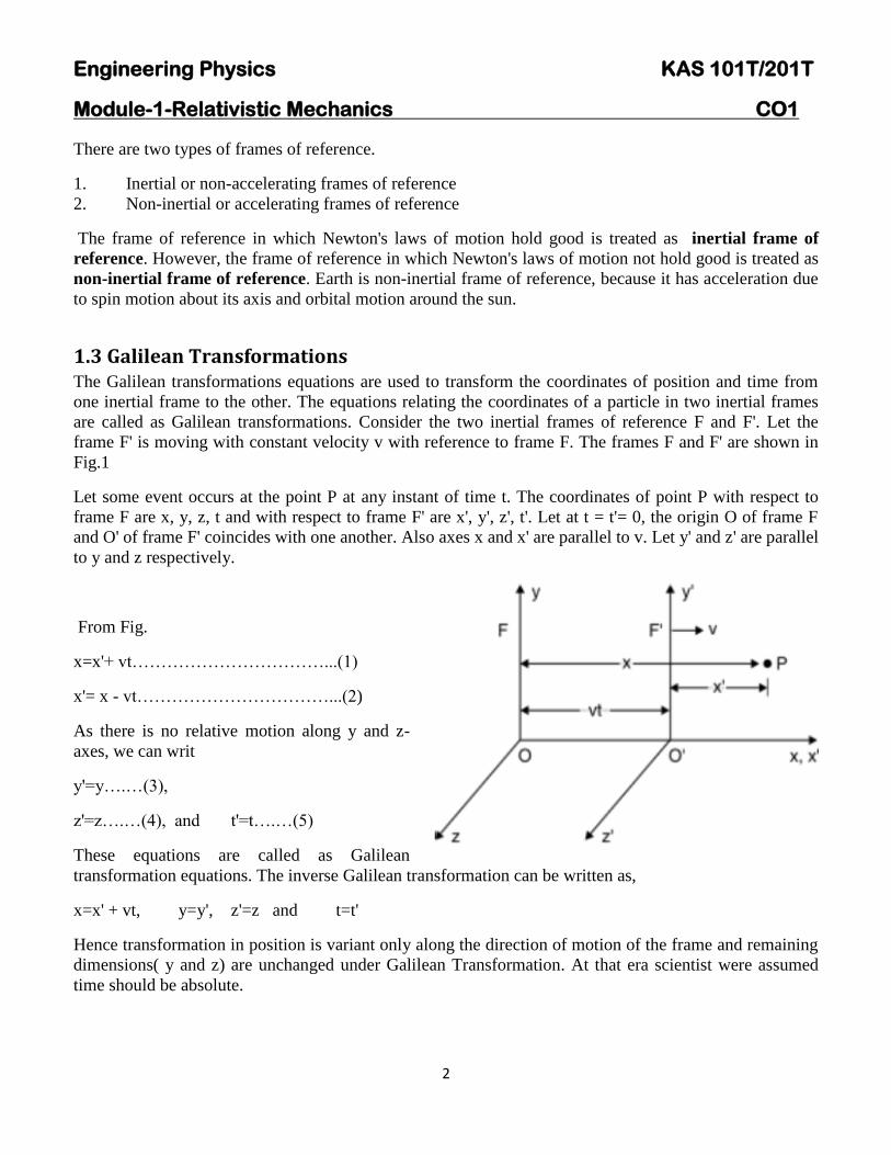
Engineering Physics KAS 101T201T
Module-1-Relativistic Mechanics CO1
2
There are two types of frames of reference
1 Inertial or non-accelerating frames of reference
2 Non-inertial or accelerating frames of reference
The frame of reference in which Newtons laws of motion hold good is treated as inertial frame of
reference However the frame of reference in which Newtons laws of motion not hold good is treated as
non-inertial frame of reference Earth is non-inertial frame of reference because it has acceleration due
to spin motion about its axis and orbital motion around the sun
13 Galilean Transformations The Galilean transformations equations are used to transform the coordinates of position and time from
one inertial frame to the other The equations relating the coordinates of a particle in two inertial frames
are called as Galilean transformations Consider the two inertial frames of reference F and F Let the
frame F is moving with constant velocity v with reference to frame F The frames F and F are shown in
Fig1
Let some event occurs at the point P at any instant of time t The coordinates of point P with respect to
frame F are x y z t and with respect to frame F are x y z t Let at t = t= 0 the origin O of frame F
and O of frame F coincides with one another Also axes x and x are parallel to v Let y and z are parallel
to y and z respectively
From Fig
x=x+ vthelliphelliphelliphelliphelliphelliphelliphelliphelliphelliphellip(1)
x= x - vthelliphelliphelliphelliphelliphelliphelliphelliphelliphelliphellip(2)
As there is no relative motion along y and z-
axes we can writ
y=yhelliphellip(3)
z=zhelliphellip(4) and t=thelliphellip(5)
These equations are called as Galilean
transformation equations The inverse Galilean transformation can be written as
x=x + vt y=y z=z and t=t
Hence transformation in position is variant only along the direction of motion of the frame and remaining
dimensions( y and z) are unchanged under Galilean Transformation At that era scientist were assumed
time should be absolute
Engineering Physics KAS 101T201T
Module-1-Relativistic Mechanics CO1
3
b) Transformation in velocities components The conversion of velocity components measured in frame F into their equivalent components in the
frame F can be known by differential Equation (1) with respect to time we get
ux=
=
( )
hence ux= ux-V
Similarly from Equation (3) and (4) we can write
uy= uy and uz= uz
In vector form
Hence transformation in velocity is variant only along the direction of motion of the frame and remaining
dimensions( along y and z) are unchanged under Galilean Transformation
c) Transformation in acceleration components
The acceleration components can be derived by differentiating velocity equations with respect to
time
ax=
( )
ax= ax
In vector form a = a
This shows that in all inertial reference frames a body will be observed to have the same acceleration
Hence acceleration are invariant under Galilean Transformation
Failures of Galilean transformation According to Galilean transformations the laws of mechanics are invariant But under Galilean
transformations the fundamental equations of electricity and magnetism have very different
forms
Also if we measure the speed of light c along x-direction in the frame F and then in the frame F
the value comes to be c = c ndash vx But according to special theory of relativity the speed of light c
is same in all inertial frames
14 Michelson-Morley Experiment ldquoThe objective of Michelson - Morley experiment was to detect the existence of stationary medium ether
(stationary frame of reference ie ether frame)rdquo which was assumed to be required for the propagation of
the light in the space
u=u ndash v
Engineering Physics KAS 101T201T
Module-1-Relativistic Mechanics CO1
4
In order to detect the change in velocity of light due to relative motion between earth and hypothetical
medium ether Michelson and Morley performed an experiment which is discussed below The
experimental arrangement is shown in Fig
Light from a monochromatic source S falls on the semi-silvered glass plate G inclined at an angle 45deg to
the beam It is divided into two parts by the semi silvered surface one ray 1 which travels towards mirror
M1 and other is transmitted ray 2 towards mirror M2 These two rays fall normally on mirrors M1 and M2
respectively and are reflected back along their original paths and meet at point G and enter in telescope In
telescope interference pattern is obtained
If the apparatus is at rest in ether the two reflected rays would take equal time to return the glass plate G
But actually the whole apparatus is moving along with the earth with a velocity say v Due to motion of
earth the optical path traversed by both the rays are not the same Thus the time taken by the two rays to
travel to the mirrors and back to G will be different in this case
Let the mirrors M1 and M2 are at equal distance l from the glass plate G Further let c and v be the
velocities at light and apparatus or earth respectively It is clear from Fig that the reflected ray 1 from
glass plate G strikes the mirror M1at A and not at A due to the motion of the earth
The total path of the ray from G to A and back will be GAG
there4 From Δ GAD (GA)2=(AA)
2+ (AD)
2(1) As (GD =AA)
If t be the time taken by the ray to move from G to A then from Equation (1) we have
(c t)2=(v t)
2 + (l)
2
Hence t=
radic
If t1 be the time taken by the ray to travel the whole path GAG then
Engineering Physics KAS 101T201T
Module-1-Relativistic Mechanics CO1
5
t1= 2t =
radic =
(
)
t1=
((
)) helliphelliphelliphelliphelliphellip(2) Using Binomial Theorem
Now in case of transmitted ray 2 which is moving longitudinally towards mirror M2 It has a velocity (c ndash
v) relative to the apparatus when it is moving from G to B During its return journey its velocity relative
to apparatus is (c + v) If t2 be the total time taken by the longitudinal ray to reach G then
T2=
( )
( ) after solving
t2=
((
)) helliphelliphelliphelliphelliphellip(3)
Thus the difference in times of travel of longitudinal and transverse journeys is
Δt = t2-t1 = =
((
))
((
))
Δt =
helliphelliphelliphelliphelliphellip(4)
The optical path difference between two rays is given as
Optical path difference (Δ) =Velocity times t = c x Δt
= c x =
Δ =
helliphelliphelliphelliphelliphellip(5)
If λ is the wavelength of light used then path difference in terms of wavelength is =
λ
Michelson-Morley perform the experiment in two steps First by setting as shown in fig and secondly by
turning the apparatus through 900 Now the path difference is in opposite direction ie path difference is
-
λ
Hence total fringe shift ΔN =
Michelson and Morley using l=11 m λ= 5800 x 10-10
m v= 3 x 10⁴ msec and c= 3 x 10
8 msec
there4 Change in fringe shift ΔN =
λ substitute all these values
=037 fringe
Engineering Physics KAS 101T201T
Module-1-Relativistic Mechanics CO1
6
But the experimental were detecting no fringe shift So there was some problem in theory calculation and
is a negative result The conclusion drawn from the Michelson-Morley experiment is that there is no
existence of stationary medium ether in space
Negative results of Michelson - Morley experiment 1 Ether drag hypothesis In Michelson - Morley experiment it is explained that there is no relative
motion between the ether and earth Whereas the moving earth drags ether alone with its motion
so the relative velocity of ether and earth will be zero
2 Lorentz-Fitzgerald Hypothesis Lorentz told that the length of the arm (distance between the pale
and the mirror M2) towards the transmitted side should be L(radic1 ndash v2c
2) but not L If this is taken
then theory and experimental will get matched But this hypothesis is discarded as there was no
proof for this
3 Constancy of Velocity of light In Michelson - Morley experiment the null shift in fringes was
observed According to Einstein the velocity of light is constant it is independent of frame of
reference source and observer
Einstein special theory of Relativity (STR)
Einstein gave his special theory of relativity (STR) on the basis of M-M experiment
Einsteinrsquos First Postulate of theory of relativity
All the laws of physics are same (or have the same form) in all the inertial frames of reference
moving with uniform velocity with respect to each other (This postulate is also called the law of
equivalence)
Einsteinrsquos second Postulate of theory of relativity
The speed of light is constant in free space or in vacuum in all the inertial frames of reference
moving with uniform velocity with respect to each other (This postulate is also called the law of
constancy)
15 Lorentz Transformation Equations
Consider the two observers O and O at the origin of the inertial frame of reference F and F respectively
as shown in Fig Let at time t = t = 0 the two coordinate systems coincide initially Let a pulse of light is
flashed at time t = 0 from the origin which spreads out in the space and at the same time the frame F starts
moving with constant velocity v along positive X-direction relative to the frame F This pulse of light
reaches at point P whose coordinates of position and time are (x y z t) and (xy z t) measured by the
observer O and O respectively Therefore the transformation
equations of x and x can be given as
x=k (x ndash v t)helliphelliphelliphelliphelliphelliphelliphelliphellip(1)
Where k is the proportionality constant and is independent of
x and t
Engineering Physics KAS 101T201T
Module-1-Relativistic Mechanics CO1
7
The inverse relation can be given as
x=k (x + v t) helliphelliphelliphelliphelliphelliphellip (2)
As t and t are not equal substitute the value of x from Equation (1) in Equation (2)
x=k [k (x ndash vt) + vt] or
=( )
t=
or t=
(
) helliphelliphelliphelliphelliphelliphelliphelliphellip(3)
According to second postulate of special theory of relativity the speed of light c remains constant
Therefore the velocity of pulse of light which spreads out from the common origin observed by observer
O and O should be same
there4 x=c t and x = cthelliphelliphelliphelliphelliphelliphelliphelliphelliphelliphelliphelliphelliphelliphellip(4)
Substitute the values of x and x from Equation (4) in Equation (1) and (2) we get
ct=k (x ndash v t) = k (ct ndash v t) or ct=kt (c ndash v) (5)
and similarly ct=k t (c + v) (6)
Multiplying Equation (5) and (6) we get
c2 t t=k
2t t (c
2 ndash v
2) hence
after solving k=
radic
(7)
Hence equation (7) substitute in equation (1) then Lorentz transformation in position will be
x=
radic
y=y z=z
Calculation of Time equation (7) substitute in equation (3)
t=
(
)
From equation ( 7)
or
then above equation becomes
t=
=
or t= (
)
Engineering Physics KAS 101T201T
Module-1-Relativistic Mechanics CO1
8
Therefore t=
radic
Hence the Lorentz transformation equations becomes
x=
radic
y=y z=z and t=
radic
Under the condition Lorentz transformation equation can be converted in to Galilean
Transformation
x=x -vt y=y z=z and t=t
16 Applications of Lorentz Transformation
161 Length contraction Consider a rod at rest in a moving frame of reference F moving along x-direction with constant velocity
v relative to the fixed frame of reference F as shown in Fig
The observer in the frame F measures the length
of rod AB at any instant of time t This length Lo
measured in the system in which the rod is at rest
is called proper length therefore Lo is given as
Lo= x2- x1 helliphelliphelliphelliphelliphelliphelliphelliphelliphelliphellip(1)
Where x1 and x2 are the coordinates of the two
ends of the rod at any instant At the same time
the length of the rod is measured by an observer
O in his frame say L then
L= x2- x1 helliphelliphelliphelliphelliphelliphelliphelliphelliphelliphellip(2)
Where x1 and x2 are the coordinates of the rod AB
respectively with respect to the frame F According to Lorentz transformation equation
x1=
radic
and x2=
radic
Hence x2- x1=
radic
By using Equations (1) and (2) we can write
Lo=
radic
Engineering Physics KAS 101T201T
Module-1-Relativistic Mechanics CO1
9
Hence L=Lo radic
helliphelliphelliphelliphelliphelliphellip(3)
From this equation Thus the length of the rod is contracted by a factor radic
as measured by observer in
stationary frame F
Special Case
If v ltltlt c then v2c
2 will be negligible in Loradic
and it can be neglected
Then equation (3) becomes L = LO
Percentage of length contraction=
162 Time dilation Let there are two inertial frames of references F and F F is the stationary frame of reference and F is the
moving frame of reference At time t=trsquo=0 that is in the start they are at the same position that is
Observers O and Orsquo coincides After that F frame starts moving with a uniform velocity v along x axis
Let a clock is placed in the frame F The time coordinate of the initial time of the clock will be t1
according to the observer in S and the time coordinate of the final tick (time) will be will be t2 according
to same observer
The time coordinate of the initial time of the clock will be t1 according to the observer in F and the time
coordinate of the final tick (time) will be will be t2 according to same observer
Therefore the time of the object as seen by
observer O in F at the position xrsquo will be
to = trsquo2 ndash trsquo1 helliphelliphelliphelliphelliphelliphelliphelliphelliphelliphelliphellip(1)
The time trsquo is called the proper time of the event
The apparent or dilated time of the same event
from frame S at the same position x will be
t = t2 ndash t1 helliphelliphelliphelliphelliphelliphelliphelliphelliphelliphelliphellip(2)
Now use Lorentz inverse transformation
equations for that is
t1 =
radic
helliphelliphelliphelliphelliphelliphelliphellip (3)
t2 =
radic
helliphelliphelliphelliphelliphelliphelliphellip (3)
Engineering Physics KAS 101T201T
Module-1-Relativistic Mechanics CO1
10
By putting equations (3) and (4) in equation (2) and solving we get
t =
radic
Substitute equation (1) in above equation
t =
radic
This is the relation of the time dilation
Special Case
If v ltltlt c then v2c
2 will be negligible in
radic
and it can be neglected
Then t = to
Experimental evidence The time dilation is real effect can be verified by the following experiment In
1971 NASA conducted one experiment in which JC Hafele as astronomer and RF Keating a physicist
circled the earth twice in a jet plane once from east to west for two days and then from west to east for
two days carrying two cesium-beam atomic clocks capable of measuring time to a nanosecond After the
trip the clocks were compared with identical clocks The clocks on the plane lost 59 10 ns during their
eastward trip and gained 273 7 ns during the westward tripThis results shows that time dilation is real
effect
163 Relativistic Addition of Velocities One of the consequences of the Lorentz transformation equations is the counter-intuitive ldquovelocity
addition theoremrdquo Consider an inertial frame Srsquo moving with uniform velocity v relative to stationary
observer S along the positive direction of X- axis Suppose a particle is also moving along the positive
direction of X-axis If the particle moves through a distance dx in time interval dt in frame S then
velocity of the particle as measured by an observer in this frame is given by
(1)
To an observer in Srsquo frame let the velocity be (by definition)
(2)
Now we have the Lorentz transformation equations
radic(
)
and
radic(
)
(3)
Taking differentials of above equations we get
Engineering Physics KAS 101T201T
Module-1-Relativistic Mechanics CO1
11
and
radic( ) (4)
Using eq (4) in eq(2) we get
(
)
( ) (5)
Or
( ) (6)
This is the the relativistic velocity addition formula If the speeds u and v are small compared to the speed
of light above formula reduces to Newtonian velocity addition formula
Inverse of the formula (6) enables us to find velocity of a particle in S frame if it is given in Srsquo frame
(6)
17 Variation of Mass with Velocity In Newtonian physics mass of an object used to be an absolute entity same in all frames One of the
major unusual consequences of relativity was relativity of mass In the framework of relativity it can be
shown that mass of an object increases with its velocity We have the following equation expressing the
variation of mass with velocity
radic( ) (1)
Where is the mass of the object at rest known as rest mass and is its velocity relative to observer
As it is clear from above equation if in agreement with common experience
Derivation
We use relativistic law of momentum conservation to arrive at eq (1) Consider two inertial frames S and
Srsquo Srsquo moving with respect to S with velocity v along positive X-axis Let two masses and are
moving with velocities ursquo and ndashursquo with respect to moving frame Srsquo
Now let us analyse the collision between two bodies with respect to frame S If u1 and u2
are velocities of two masses with respect to frame S then from velocity addition theorem
and
(2)
Engineering Physics KAS 101T201T
Module-1-Relativistic Mechanics CO1
12
At the time of collision two masses are momentarily at rest relative to frame Srsquo but as seen from frame S
they are still moving with velocity v Since we assume momentum to be conserved even in relativity
theory as seen from S frame
Momentum before collision = momentum after collision
( ) (3)
Substituting the values of u1 and u2 from equation (2) eq(3) becomes
(
) + (
) = ( )
Rearranging the terms
(
) = (
)
( ( )
) ) = (
( )
)
Or ( ( )
) ) = (
( )
)
(4)
Now using set of equations (2) we can find RHS of equation to be equal to
radic
If u2 = 0 ie m2(= m0say) is at rest with respect to S frame above equation reduces to
radic
We could have chosen two masses to be identical In that case m0 will also be the rest mass of So
we can apply above formula to a single with rest mass and moving mass m related by
radic
Engineering Physics KAS 101T201T
Module-1-Relativistic Mechanics CO1
13
This shows that mass of a body increases with its velocity
18 Mass- Energy Equivalence In Newtonian Physics mass and energy are assumed to be quite different entities There is no mechanism
in Newtonian set up how mass and energy can be converted into each other Like many other it is one of
unusual consequences of special relativity that mass and energy are inter-convertible into each other and
hence are equivalent
Einsteinrsquos Mass- energy relation ( ) (Derivation)
Consider a particle of mass m acted upon by a force F in the same direction as its velocity v If F
displaces the particle through distance ds then work done dW is stored as kinetic energy of the particle
dK therefore
(1)
But from Newtonrsquos law
( )
(2)
Using (2) in (1)
Or (3)
Now we have
radic
(
) (4)
Taking the differential
( )(
) (
)
(
)
But ( )
( )
(
)
Or
( )
or ( ) (5)
Using eq (5) in eq (3)
Engineering Physics KAS 101T201T
Module-1-Relativistic Mechanics CO1
14
( )
Let the change in kinetic energy of the particle be K as its mass changes from rest mass to to
effective mass m then
int int
( ) = (
radic
)
This is the relativistic expression for kinetic energy of a particle It says that kinetic energy of a particle is
due to the increase in mass of the particle on account of its relative motion and is equal to the product of
the gain in mass and square of the velocity of light can be regarded as the rest energy of the
particle of rest mass The total energy E of a moving particle is the sum of kinetic energy and its rest
mass energy
( )
Or
This is the celebrated mass- energy equivalence relation This equation is so famous that even common
men identify Einstein with it
Significance This equation represents that energy can neither be created nor be destroyed but it can
change its form
Evidence show its validity
First verification of the was made by Cock-croft and Walton
(70166 amu) (10076 amu) (40026 amu)
Mass defect = (70166 amu+10076 amu) -2x (40028 amu)
=00186 amu
= 00186 x 166 X 10-27
kg
= 00186 x 166 X 10-27
x ( )
=
=( )
( )
=
Engineering Physics KAS 101T201T
Module-1-Relativistic Mechanics CO1
15
( a huge amount of energy release)
19 Relation between Energy and Momentum
a) Relation between total Energy and Momentum
Sconce we know that
radic
Squaring both side
(
)=
=
Science =
substitute in above equation
(
)
= after solving
This is the relation between relativistic total energy and momentum of the particle
b) Relation between Kinetic Energy and Momentum
Science we know that ------------------------(1)
Also we know that
Squaring both side
( ) -----------------------(2)
From equation (1) and (2) we get
= (
)
=
After solving
Engineering Physics KAS 101T201T
Module-1-Relativistic Mechanics CO1
16
radic
Where = kinetic energy
110 Mass-less Particle Zero Rest Mass Particles A particle which has zero rest mass( ) is called massless particle
We have the energy-momentum relation
radic ( ) (1)
For a massless particle
Therefore or (2)
But therefore
Which implies
This says that a massless particles always move with the speed of light Energy and momentum of a
massless particle is given by equation (2) Massless particles can exist only as long as the move at the
speed of light Examples are photon neutrinos and theoretically predicted gravitons
Numerical Problems
Question 1 Show that the distance between any two points in two inertial frame is invariant under
Galilean transformation
Answer Consider two frame of reference S and frame moving with constant velocity relative
to frame S in positive X-direction
Point A and B placed in frame S and their co-ordinate relative O are ( ) and ( )
After time the coordinate of A and B relative to observer from frame will be ( )
and( )
Using Galilean Transformation
and
and
Engineering Physics KAS 101T201T
Module-1-Relativistic Mechanics CO1
17
Now distance between two points from frame will be
=radic( ) ( ) ( )
Substitute all values then
=radic( ) ( ) ( )
After simplification
=radic( ) ( ) ( ) ie
=
This show that distance between two points is invariant under Galilean Transformation
Question 2 Show that the relativistic form of Newtonrsquos second law when is parallel to
=
(
)
Answer Science we know that
=
(
radic
)=[ ( (
)
)]
= [
(
)
(
) (
)
(
)]
=
[(
)
(
)
]
=
(
)
+
=
(
)
it is relativistic Newtonrsquos second law
Engineering Physics KAS 101T201T
Module-1-Relativistic Mechanics CO1
18
If then
=
= (because at )
So it can also be written as =
Question 3 A particle of rest mass moves with speed
radic Calculate its mass momentum total energy
and kinetic energy
Answer Science we know that
radic
=
radic
= radic =141
The momentum of the particle is given by
radic =
Total energy of the particle
=
Kinetic energy
= -
=
Question 4 A man weight 50 kg on the earth when he is in a rocket ship in flight his mass is 505 kg ass
measured by an observer on earth What is the speed of rocket
Answer Given that
=50 kg
radic(
)
substitute all values and after solving
ms
Question 5 Compute the mass m and speed of an electron having kinetic energy Given rest
mass of electron
Answer Given that
Engineering Physics KAS 101T201T
Module-1-Relativistic Mechanics CO1
19
Kinetic energy( ) ( )
Kinetic energy( ) ( )
hence
substitute all values and after solving
=
Using the relation
radic(
)
where = and
Then after solving
Question 6 Calculate the amount of work to be done to increase the speed of an electron from 06c to
08c Given that rest mass energy of electron ( )
Answer
Kinetic energy( ) ( ) =(
radic(
)
)
Where
For speed 06c For speed 08c
=(
radic( ( )
)
) =(
radic( ( )
)
)
= =
Hence The amount of work to be done(electron increase the speed 06c to 08c)=
=
Engineering Physics KAS 101T201T
Module-2-Electromagnetic Field Theory CO2
20
21 Continuity equation for current density Statement Equation of continuity represents the law of conservation of charge The charge flowing out
through a closed surface from some volume is equal to the rate of decrease of charge within the volume
hellip (1)
Where I is current flowing out through the surface of a volume and
is the rate of decrease of charge
within the volume
Again we know ∯ and q= intintintρdv
where J is the Conduction current density an ρ is the volume charge density
Substituting the expression of I and q in equation (1)
∯ ∭
hellip (2)
Now applying Gaussrsquos Divergence Theorem to LHS of above equation
∭ ∭
As the two volume integrals are equal so their integrands are also equal
Thus
This is continuity equation for time varying fields
Equation of Continuity for Steady Currents As ρ does not vary with time for steady currents that is
So
This is the continuity equation for steady currents
Engineering Physics KAS 101T201T
Module-2-Electromagnetic Field Theory CO2
21
22 Differential form of Maxwellrsquos equations
221 First equation (Gauss Law of Electrostatic)
Gauss law of electrostatic states that the total electric flux E coming out from a closed surface is equal to
1ε0 times the net charge enclosed by the surface ie ∯
∯ =intintintρdv hellip (1)
Applying Gaussrsquos Divergence theorem to change LHS of equation (1) ∯ =intv (nablaD) dv
Using this equation in equation (1) we will get
intintint (nablaD)dv=intintintρdv
As two volume integrals are equal so their integrands are also equal
Thus nablaD=ρ hellip (2)
The above equation is the Differential form of Maxwellrsquos first equation
222 Second equation(Gauss Law of Magnetostatic)
Gauss law of magnetostatic states that the total magnetic flux φm coming out through surface of a volume
is always equal to zero
φm=∯ hellip(3)
Applying Gaussrsquos Divergence theorem ∯ =intintint(nablaB)dv
Putting this in equation (3) intintint (nablaB)dv =0
Thus nablaB=0 hellip(4)
This equation (4) is differential form of Maxwellrsquos second equation
223 Third Equation(Faradayrsquos Law of Electromagnetic Induction)
1 It states that if there is a change of magnetic flux linked with a circuit then electromotive force (emf) is
induced in the circuit This induced emf lasts as long as the change in magnetic flux continues
Engineering Physics KAS 101T201T
Module-2-Electromagnetic Field Theory CO2
22
2 The magnitude of induced emf is equal to the rate of change of magnetic flux linked with the circuit
Therefore induced emf
hellip(5)
Where φm= intintBds hellip(6)
Here negative sign indicates the induced emf set up a current in such a direction that the magnetic effect
produced by it opposes the cause producing it
Again we know emf is the closed line integral of the non-conservative electric field generated by the
battery
That is emf=∮ hellip(7)
Putting equations (6) and (7) in equation (5) we get
∮ = ndash intint
ds hellip(8)
Using Stokersquos theorem to the LHS of equations (8) ∮ = intint (nabla x E)ds
Substituting above equation in equation (8) we get
intint (nabla x E)dS = -intint
ds
Two surface integral are equal only when their integrands are equal
Thus nabla x E = ndash
hellip(9)
This is the differential form of Maxwellrsquos 3rd
equation
224 Forth Equation (Modified Amperersquos Circuital Law)
To come to the Maxwellrsquos 4th
equation let us first discuss Amperersquos circuital law
Amperersquos circuital law This law states that the line integral of the magnetic field H around any closed
path or circuit is equal to the current enclosed by that path
That is ∮ =I
Engineering Physics KAS 101T201T
Module-2-Electromagnetic Field Theory CO2
23
If J is the current density then I=intintJds
This implies that ∮ =intintJds hellip(10)
Applying Stokersquos theorem to LHS of above equation ∮ =intint(nablaxH)ds
Substituting above equation in equation (10) we will get intint(nablaxH)ds =intintJds
Two surface integrals are equal only if their integrands are equal
Thus nablax H=J hellip(11)
This is the differential form of Amperersquos circuital Law for steady currents
Now taking divergence on both side of equation (10) nabla(nablaxH)= nablaJ
As divergence of the curl of a vector is always zero therefore nabla(nablaxH)=0
It means nablaJ=0
Now this is continuity equation for steady current but not for time varying fields as equation of
continuity for time varying fields is
So Amperersquos circuital law is incomplete valid only for steady state current This is the reason that led
Maxwell to modify Amperersquos circuital law
Modification of Amperersquos circuital law Maxwell modified Amperersquos law by giving the concept of
displacement current and displacement current density for time varying fields
He considered that equation (10) for time varying fields can be written as nablaxH=J + Jd hellip (12)
By taking divergence on both side of equation (12) we will get nabla (nabla xH)= nablaJ+ nablaJd
As the divergence of curl of a vector is always zero therefore nabla (nabla xH)= 0
So nabla (J+Jd)=0 Or nabla J= -nablaJd
But from equation of continuity for time varying fields
Engineering Physics KAS 101T201T
Module-2-Electromagnetic Field Theory CO2
24
From the above two equations of j we get
nabla Jd = ( )
hellip (13)
As from Maxwellrsquos first equation nablaD=ρ
Now from equation (13) we can write
Using the above equation in equation (12) we get
nabla x H=J +
hellip(14)
Here
=Displacement current density
The equation (14) is the Differential form of Maxwellrsquos fourth equation or Modified Amperersquos circuital
law
23 Integral form of Maxwellrsquos equations
231 First Equation
Gauss law of electrostatic states that the total electric flux E coming out from a closed surface is
equal to 1ε0 times the net charge enclosed by the surface ie
∯ hellip(1)
Let ρ is the volume charge density distributed over a volume V
Therefore q=int ρ dv
So ∯
hellip(2)
This equation is the integral form of Maxwellrsquos first equation or Gaussrsquos law in electrostatics
232 Second equation
Gauss law of magnetostatic states that the total magnetic flux φm coming out through surface of a volume
is always equal to zero ie
φm=∯ hellip(3)
Engineering Physics KAS 101T201T
Module-2-Electromagnetic Field Theory CO2
25
The above equation is the intergal form of Maxwellrsquos second equation
The above equation also suggest that magnetic monopole does not exist
233 Third Equation
1 It states that if there is a change of magnetic flux linked with a circuit then electromotive force (emf) is
induced in the circuit This induced emf lasts as long as the change in magnetic flux continues
2 The magnitude of induced emf is equal to the rate of change of magnetic flux linked with the circuit
Therefore induced emf
hellip(4)
Where φm= intintBds hellip(5)
Here negative sign indicates the induced emf set up a current in such a direction that the magnetic effect
produced by it opposes the cause producing it
Again we know emf is the closed line integral of the non-conservative electric field generated by the
battery
That is emf=∮ hellip(6)
Using equations (5) and (6) in equation (4) we get
∮ = ndash intint
ds hellip(7)
The above equation is the integral form of Maxwellrsquos third Equation or Faradayrsquos law of
electromagnetic induction
234 Fourth equation
The line integration of the magnetic field H around a closed path or circuit is equal to the conductions
current plus the time derivative of electric displacement through the surface bounded by the closed path
ie
∮ =∬(
) (8)
The above equation is the integral form of Maxwellrsquos fourth equation
Engineering Physics KAS 101T201T
Module-2-Electromagnetic Field Theory CO2
26
25 Displacement Current
According to Maxwell not only conduction current produces magnetic field but also time varying electric
field produces magnetic field This means that a changing electric field is equivalent to a current which
flows as long as electric filed is changing This is current only in the sense that it produces same magnetic
effect as conduction current does there is no actual flow of electron
If E is the electric field developed between the plates of surface area A Then the displacement current is
given by
26 Electromagnetic wave Equation in Free Space
Now in free space there is no charge so charge density ρ=0 and current will also be zero Thus current
density J is also equal to zero
Hence Maxwellrsquos equation in free space is given by
hellip(1) where ( )
hellip(2)
hellip(3) where ( )
hellip(4) where ( )
261 Maxwellrsquos Electromagnetic wave Equation in Free Space for the field vector E
we take curl on both side of Maxwellrsquos 3rd
equation represented in equation (3)
( )
( ) ( )
[(using vector identity ( ) ( ) ]
Now from equation (1) and (4) in the above equation
Engineering Physics KAS 101T201T
Module-2-Electromagnetic Field Theory CO2
27
(
)
Or
hellip(5)
Similarly we can find an equation for the field vector B when we take the Maxwellrsquos 4th
and repeat the
process of field vector E
hellip(6)
Equation (5) and (6) is the guiding equation for field vector E and B respectively in free space
Thus we can see that time varying electric field produces magnetic field and time varying magnetic field
produces electric filed and follow the above guiding equation Comparing the above equation with the
standard wave equation
-------(7)
Compare equation (6) and (7) we get
radic radic
radic
Because
Hence = c
Hence this field vectors propagates in free space with the speed of light So from here Maxwell
concluded that light is an electromagnetic wave
27 Electromagnetic wave Equation in non-conducting medium
Now in non-conducting medium there is no free charge so current density J and total charge inside the
material is zero so charge density ρ is also equal to zero Maxwellrsquos equation in a non-conducting
medium of permittivity and permeability is reduces to
Engineering Physics KAS 101T201T
Module-2-Electromagnetic Field Theory CO2
28
hellip(1) where ( )
hellip(2)
hellip(3) where ( )
hellip(4) where ( )
271 Maxwellrsquos Electromagnetic wave Equation in Free Space for the field vector E
we take curl on both side of Maxwellrsquos 3rd
equation represented in equation (3)
( )
( ) ( )
[(using vector identity ( ) ( ) ]
Now using equation (1) and (4) in the above equation
(
)
Or
hellip(5)
Similarly we can find an equation for the field vector B when we take the Maxwellrsquos 4th
and repeat the
process of field vector E
hellip(6)
Equation (5) and (6) is the guiding equation for field vector E and B respectively in non-conducting
medium
Comparing the above equation with the standard wave equation
----------(7)
Engineering Physics KAS 101T201T
Module-2-Electromagnetic Field Theory CO2
29
we can see that this field vectors propagate in non-conducting medium with a speed
radic
radic
radic As 119888
radic
For non-magnetic medium 119903=1
So
radic
here radic 119903 119899 is the refractive index of the medium
Hence electromagnetic wave propagate in non-conducting medium with a speed
times the speed of
electromagnetic wave in free space
28 Transverse nature of electromagnetic wave
Science we know that the plane electromagnetic wave equation are
---(1)
---(2)
Solution of these wave equation considering the propagation of the wave in any arbitrary direction of
three dimensional space is given by
( 119903 ) (3)
( 119903 ) hellip(4)
Where E0 and B0 are the amplitudes of electric and magnetic field respectively and is propagation vector
given by = 2πλ = 2πνc = ωc
Now Maxwellrsquos first and second equation in free space is
nabla =0 hellip(5)
nabla hellip(6)
Engineering Physics KAS 101T201T
Module-2-Electromagnetic Field Theory CO2
30
Where nabla
and = 119910 119911
Putting the above expressions in L H S of equation (5)
nabla = (
) ( 119903 ) ------ (7)
Where k ky kz
and 119903 = y
So 119903 = k yky kz
Thus equation (7) can be written as
= (
)( 119910 119911
) exp ί( k yky kz )- +
=
[ exp ί ( k yky k
z )
- +]+
[ 119910exp ί ( k yky k
z )
- +]+
[ 119911
exp ί ( k yky kz )
- +]
=(ί k ) exp ί ( k yky kz )
- + +(ίky) 119910exp ί ( k yky k
z) - + +(ίk
z )
119911 exp ί ( k yky k
z )
- +
= ί[ k + 119910ky+ 119911 k
z] exp ί ( k yky k
z) - +
= ί[( k ky kz )( 119910 119911
)] exp ί ( k yky k
z )
- +
= ί( )exp(( 119903 )= ί
= ί using equation (3)
Now putting the value of in equation (5)
= ί
Or helliphellip (8)
Similarly putting equation (4) in equation (6) we will get hellip(9)
Equation (8) amp (9) suggest that electric and magnetic field vectors are perpendicular to propagation
vector So we can say that electromagnetic waves are transverse in nature
Again using Maxwellrsquos 3rd
and 4th
equations in free space are
hellip(10)
Engineering Physics KAS 101T201T
Module-2-Electromagnetic Field Theory CO2
31
hellip(11)
Now if we put the expression of from equation (3) in above Maxwellrsquos equation (equation No 10) then
we can write
ί [ ] =
( 119903 )]
= -(- ) ( 119903 )
= hellip(12)
Similarly putting the expression of from equation (4) in equation (12) we will get
= - -----(13)
From equation (12) we can say magnetic field vector is perpendicular to both amp and from (13) we
can say Electric field vector is perpendicular to both Thus electric field vector magnetic field
vector and propagation vector are mutually perpendicular to each other
Characteristic Impedance
As amp are perpendicular to each other and amp are mutually perpendicular so from
equation (12)
=
Or
Or
=
νλ = c
Thus
= c
Or
= micro
0 c and 119888
radic
Or
=
radic
= radic
= 37672 Ω
The quantity
= Z
0 = 37672Ω is known as characteristic Impedance or Intrinsic Impedance of free
space
Engineering Physics KAS 101T201T
Module-2-Electromagnetic Field Theory CO2
32
29 Energy in an electromagnetic field
The Energy of electromagnetic Wave is the sum of electric (E) and magnetic (B) field energy
The electric energy per unit volume is given by UE
The magnetic energy per unit volume is given by UB
So the total energy per unit volume in electromagnetic wave is
U =
As
and
radic So U =
+
=
+
= Ɛ0E
2
Therefore energy per unit volume in electromagnetic wave is U = Ɛ0E2
210 Skin Depth
Skin depth or depth of penetration is defined as the depth in which the strength of electric field associated
with electromagnetic wave reduces to 1e times of its initial value The figure below shows the variation
of field vector E with distance of electromagnetic wave inside a conducting medium and the value of skin
depth inside a good conductor is given by radic
Here is the conductivity of the medium and
is angular frequency of the electromagnetic wave
Engineering Physics KAS 101T201T
Module-2-Electromagnetic Field Theory CO2
33
211 Poynting vector and Poynting Theorem
Poynting vector When electromagnetic wave propagates through space it carries energy with it The
amount of energy passing through unit area in the perpendicular to direction of propagation of the
electromagnetic wave per second is given by S = E x H
This quantity S is called Poynting vector E electric field vector and H is magnetic field vector of the
electromagnetic wave The direction of S is perpendicular to E and H and in the direction of vector E x H
Theorem Consider Maxwellrsquos fourth equation (Modified Amperersquos Circuital Law) that is
nabla x H = J + ε dEdt
or J = (nabla x H) ndash ε dEdt
The above equation has the dimensions of current density Now to convert the dimensions into rate of
energy flow per unit volume take dot product of both sides of above equation by E that is
E J = E (nabla x H) ndash εE dEdt (1)
Now using vector Identity
nabla (E x H) = H (nabla x E) ndash E (nabla x H)
or E (nabla x H) = H (nabla x E) ndash nabla ( E x H )
By substituting value of E (del x H) in equation (1) we get
Engineering Physics KAS 101T201T
Module-2-Electromagnetic Field Theory CO2
34
E J =H(nabla x E) ndash nabla(E x H) ndash εEdEdt (2)
Also from Maxwellrsquos third equation (Faradayrsquos law of electromagnetic induction)
nabla x E = μdHdt
By substituting value of nabla x E in equation (2) we get
E J =μHdHdt ndash εE dEdt ndash nabla (E x H) (3)
We can write
H dHdt = 12 dH2dt (4a)
E dEdt = 12 dE2dt (4b)
By substituting equations 4a and 4b in equation 3 we get
E J = -μ2 dH2dt ndash ε2 dE
2dt ndash nabla (E x H)
E J = -d(μH22 + εE
2 2)dt ndash nabla (E x H)
By taking volume integral on both sides we get
intintintE JdV = -d[intintint (μH22 + εE
2 2)dV]dt ndash intintint nabla (E H) dV (5)
Applying Gaussrsquos Divergence theorem to second term of RHS to change volume integral into surface
integral that is
intintint nabla(E H) dV = ∯( )
Substitute above equation in equation (5)
intintintE JdV = -d[intintint (μH22 + εE
2 2)dV]dt ndash ∯ (6)
Engineering Physics KAS 101T201T
Module-2-Electromagnetic Field Theory CO2
35
or ∯ = -intintint[d(μH22 + εE
2 2)dt] dV ndashintintintE J dV
Interpretation of above equation
LHS Term
∯ rarr It represents the rate of outward flow of energy through the surface of a volume V and
the integral is over the closed surface surrounding the volume This rate of outward flow of power from a
volume V is represented by
∯ ∯
where Poynting vector S = E H
Inward flow of power is represented by ∯ ∯
RHS First Term
-intintint[d(μH22 + εE
2 2)dt] dV rarr If the energy is flowing out of the region there must be a
corresponding decrease of electromagnetic energy So here negative sign indicates decrease
Electromagnetic energy is the sum of magnetic energy μH22 and electric energy εE
2 2 So first term of
RHS represents rate of decrease of stored electromagnetic energy
RHS Second Term
ndashintintintE J dV rarrTotal ohmic power dissipated within the volume
So from the law of conservation of energy equation (6) can be written in words as
Rate of energy dissipation in volume V = Rate at which stored electromagnetic energy is decreasing in V
+ Inward rate of flow of energy through the surface of the volume
212 Radiation Pressure
The electromagnetic waves exert a ldquoRadiation Pressurerdquo on a surface due to absorption and reflection of
the electromagnetic wave An object absorbing an electromagnetic wave would experience a force in the
direction of propagation of the wave During these processes momentum is exchanged between the
surface and the electromagnetic wave
Engineering Physics KAS 101T201T
Module-2-Electromagnetic Field Theory CO2
36
Consider an em wave of average energy density ltugt and average poynting vector ltSgt be incident
normally on a surface then the radiation pressure P exerted by em waves on this surface is
hellip (1)
where ltFgt is the average force exerted by the em waves
Now using Newtonrsquos Second Law
hellip(2)
Where ltPgt is the momentum of incident em waves
For electromagnetic wave we know that
hellip(3)
Putting equation ( 3 ) in ( 2 )
hellip(4)
Since S= PowerArea and Power = EnergyTime
Therefore S=
So we can write
hellip(5)
Now using equation ( 5 ) in ( 4 )
119888 hellip(6)
Using equation ( 6 ) in ( 1 ) radiation pressure due to absorption of electromagnetic wave is
Engineering Physics KAS 101T201T
Unit-III-Quantum Mechanics CO3
BLACKBODY RADIATION SPECTRUM
A blackbody is an object that absorbs all of the radiation that it receives (that is it does not reflect any light nor does it allow any light to pass through it and out the other side) The energy that the blackbody absorbs heats it up and then it will emit its own radiation The only parameter that determines how much light the blackbody gives off and at what wavelengths is its temperature There is no object that is an ideal blackbody but many objects (stars included) behave approximately like blackbodies Other common examples are the filament in an incandescent light bulb or the burner element on an electric stove As you increase the setting on the stove from low to high you can observe it produce blackbody radiation the element will go from nearly black to glowing red hot
Plot of the spectrum of a blackbody with different temperatures
The spectrum of a blackbody is continuous (it gives off some light at all wavelengths) and it has a peak at a specific wavelength The peak of the blackbody curve in a spectrum moves to shorter wavelengths for hotter objects
Rayleigh-Jeans radiation law
The Rayleigh-Jeans Radiation Law was a useful but not completely successful attempt at establishing the functional form of the spectra of thermal radiation The energy density uν per unit frequency interval at a frequency ν is according to the The Rayleigh-Jeans Radiation
(1) dνuν = c38πν kT2
where k is Boltzmanns constant T is the absolute temperature of the radiating body and c is the speed of light in a vacuum This formula fits the empirical measurements for low frequencies but fails increasingly for higher frequencies The failure of the formula to match the new data was called the ultraviolet catastrophe The significance of this inadequate so-called law is that it provides an asymptotic condition which other proposed formulas such as Plancks need to satisfy It gives a value to an otherwise arbitrary constant in Plancks thermal radiation formula
1
user
Textbox
37
Engineering Physics KAS 101T201T
Unit-III-Quantum Mechanics CO3
Stefanrsquos Law
The spectrum of radiation emitted by a solid material is a continuous spectrum unlike the line spectrum emitted by the same material in gaseous form The peak frequency of the emitted spectrum increases with the temperature of the solid body as does the total power radiated
Definition According to the Stefan-Boltzmann law the total power radiated by an ideal emitter (perfect blackbody) is proportional to the fourth power of the absolute temperature
P = AσT4
Where P = total power radiated from the blackbody
A = surface area of the blackbody σ = Stefan-Boltzmann constant
T = Absolute temperature of the blackbody To generalize
P = 120692AσT4
Where 120692 is the emissivity And
120692 = 1 for black body 120692 lt 1 for grey bodies (not perfect blackbody
Wienrsquos Displacement Law
When the temperature of a blackbody radiator increases the overall radiated energy increases and the peak of the radiation curve moves to shorter wavelengths When the maximum is evaluated from the Planck radiation formula the product of the peak wavelength and the temperature is found to be a constant
λmT = 2898 x 10-3mK (2)
This relationship is called Wiens displacement law and is useful for the determining the temperatures of hot radiant objects such as stars and indeed for a determination of the temperature of any radiant object whose temperature is far above that of its surroundings
Refhttphyperphysicsphy-astrgsueduhbasewienhtml
2
user
Textbox
38
Engineering Physics KAS 101T201T
Unit-III-Quantum Mechanics CO3
Wienrsquos Distribution law
William Wien used thermodynamics to show that the spectral energy density of a blackbody between the wavelength range 120524 and 120524+d120524 is given by
E120582119889120582 = 119860 119891(120582119931) 119889120582 hellip (1)
1205825
Wien found using the Maxwell-Boltzmann distribution law for the speed of atoms (or molecules) in a gas that the form of the function f (120524T) was
119891(120582119931) = 119942 -120572 120582119931 hellip (2) And therefore
E120582119889120582 = 119860 120582-5 119942 -120572 120582119931119889120582 hellip (3) Where A and 120514 are constants to be determined Equation (3) is known as Wienrsquos Distribution Law Assumption of Quantum Theory of Radiation
The distribution of energy in the spectrum of radiations of a hot body cannot be explained by applying the classical concepts of physics Max Planck gave an explanation to this observation by his Quantum Theory of Radiation His theory says
a) The radiant energy is always in the form of tiny bundles of light called quanta ie the energy is absorbed or emitted discontinuously
b) Each quantum has some definite energy E=hν which depends upon the frequency (ν) of the radiations where h = Planckrsquos constant = 6626 x10-34Js
c) The energy emitted or absorbed by a body is always a whole multiple of a quantum ie nhνThis concept is known as quantization of energy
Planckrsquos Law(or Planckrsquos Radiation Law)
Plancks radiation law is derived by assuming that each radiation mode can be described by a quantized harmonic oscillator with energy En = nhν
Let N0 be the number of oscillators with zero energy ie E0 (in the so-called ground-state) then the numbers in the 1st 2nd 3rd etc levels (N1 N2 N3hellip) are given by
N exp N 1 = 0 ( kTminusE1 ) N exp N exp N 2 = 0 ( kT
minusE2 )N 3 = 0 ( kTminusE3 )
3
user
Textbox
39
Engineering Physics KAS 101T201T
Unit-III-Quantum Mechanics CO3
But since En = nhν
N exp N 1 = 0 ( kTminushν) N exp N exp N 2 = 0 ( kT
minus2hν) N 3 = 0 ( kTminus3hν)
The total number of oscillators N = N0 + N1 + N2 + N3helliphelliphelliphelliphellip
The total energy E = + + +hellipνN xp h 0 exp e ( kTminushν) exp 2hνN 0 ( kT
minus2hν) exp 3hνN 0 ( kTminus3hν)
The avg energy lt E gt = EN
lt E gt = N 1+exp xp ( ) +exp xp ( ) +hellip0[ e kTminushν e kT
minus2hν ]hνN exp xp ( ) + ( ) + ( ) +hellip0[ e kT
minushνkT
minus2hνkT
minus3hν ]
lt E gt = hν xp ( ) exp e kTminushν
1minusexp xp ( ) [ e kTminushν ]
(4)lt E gt = hν exp xp ( )minus1 [ e hν
kT ]
According to Rayleigh-Jeans law using classical physics the energy density uνper frequency interval was given by
(5)dνuν = c38πν kT 2
where kT was the energy of each mode of the electromagnetic radiation We need to replace the kT in this equation with the average energy for the harmonic oscillators that we have just derived above So we re-write the energy density as
(6)dνuν = c38πν2 hν
exp xp ( )minus1 [ e hνkT ]
Comparison of Rayleigh Jeans Wienrsquos amp Planckrsquos Radiation Laws for the blackbody radiation spectrum
4
user
Textbox
40
Engineering Physics KAS 101T201T
Unit-III-Quantum Mechanics CO3
WAVE PARTICLE DUALITY
In physics and chemistry wave-particle duality holds that light and matter exhibit properties of both waves and of particlesA central concept of quantum mechanics duality addresses the inadequacy of conventional concepts like particle and wave to meaningfully describe the behaviour of quantum objects
Publicized early in the debate about whether light was composed of particles or waves a wave-particle dual nature soon was found to be characteristic of electrons as well The evidence for the description of light as waves was well established at the turn of the century when the photoelectric effect introduced firm evidence of a particle nature of light as well On the other hand the particle properties of electron was well documented when the DeBroglie hypothesis and the subsequent experiments by Davisson and Germer established the wave nature of the electron
Refhttphyperphysicsphy-astrgsueduhbasemod1html
De Broglie Matter Waves
De Broglie Hypothesis
In 1924 Lewis de-Broglie proposed that matter has dual characteristic just like radiation His concept about the dual nature of matter was based on the following observations-
(a) The whole universe is composed of matter and electromagnetic radiations Since both are forms of energy so can be transformed into each other
(b) The matter loves symmetry As the radiation has dual nature matter should also possess dual character
5
user
Textbox
41
Engineering Physics KAS 101T201T
Unit-III-Quantum Mechanics CO3
According to the de Broglie concept of matter waves the matter has dual nature It means when the matter is moving it shows the wave properties (like interference diffraction etc) are associated with it and when it is in the state of rest then it shows particle properties Thus the matter has dual nature The waves associated with moving particles are matter waves or de-Broglie waves
(7)λ = hmv
where λ = de Broglie wavelength associated with the particle h = Planckrsquos constant m = relativistic mass of the particle and v = velocity of the particle
Phase velocityGroup Velocity (MATTER WAVES) The phase velocity of a wave is the rate at which the phase of the wave propagates in space This is the velocity at which the phase of any one frequency component of the wave travels Let P be a phase point located on a travelling wave represented by the equation Asin(kx t) y = minus ω where πλ is the wave number k = 2 ω πν is the angular f requency = 2
then the phase velocity is given by = vp λ ν = k
ω (8) Also and E=mc2ν = h
E (9) and λ = p
h v p = m (10)
Substituting (9) and (10) in (8) we obtain = = vp pE
vctimesc
The velocity of the phase point will be the same as the wave velocity As already mentioned v = velocity of the particle associated with the waveTherefore For Photon v = c so in vacuum vp = c For other particles v lt c but vpgt c which has no physical significance For a physically significant representation of matter waves we require a wave packet to be associated with the moving particle(or body)
6
user
Textbox
42
Engineering Physics KAS 101T201T
Unit-III-Quantum Mechanics CO3
The velocity of the wave packet is called Group Velocity 119907119892 = 119889120596 = 119889119864 (11)
119889119896 119889119901
BORN INTERPRETATION OF THE WAVE FUNCTION AND ITS SIGNIFICANCE Matter waves are represented by a complex function Ψ (xt) which is called a wave function The wave function is not directly associated with any physical quantity but the square of the wave function represents the probability density in a given region The wave function should satisfy the following conditions (i) Ψ should be finite (ii)Ψ should be single valued (iii) Ψ and its first derivative should be continuous (iv) Ψ should be normalizable
2 dV = 1 where V = volume in which the particle is expected to be foundint
VΨ| |
SCHRODINGERrsquoS WAVE EQUATION
TIME INDEPENDENT SCHRODINGERrsquoS EQUATION
The classical wave equation that describes any type of wave motion can be given as
= partx2part y(xt) 2 1
v2 partt2part y(xt)2
Where y is a variable quantity that propagates in lsquox lsquo direction with a velocity lsquovrsquo Matter waves should also satisfy a similar equation and we can write the equation for matter waves as
= (17)partx2part ψ(xt) 2 1
v2 partt2part ψ(xt)2
We can eliminate the time dependence from the above equation by assuming a suitable form of the wave function and making appropriate substitutions
7
user
Textbox
43
Engineering Physics KAS 101T201T
Unit-III-Quantum Mechanics CO3
(x ) ψ (x)e ψ t = 0minusiωt (18)
Differentiate eqn (18) wrt lsquoxrsquo successively to obtain
= (19)partx2part ψ(xt) 2
partx2part ψ (x) 2
0 eminusiωt
Differentiate eqn (18) wrt lsquotrsquo successively to obtain
= (20)partt2part ψ(xt) 2
minus ω) ψ (x)( i 20 eminusiωt
Substituting (19) and (20) in equation (17)
= = (21)partx2part ψ (x) 2
0 minus v2ω2 (x) ψ0 ψ (x) minus k2
0
= 0partx2part ψ (x) 2
0 ψ (x) + k20 (22)
Now we know the total energy lsquoE of the particle is the sum of its kinetic energy and potential energy
ie + V rArr (23)E = 2mp2
2m(E ) p2 = minus V
Also and rArr (24)k = λ2π λ = p
h k2 = h24π p2 2
Substituting (23) in (24) in then substituting result in (22) we get
= 0partx2part ψ (x) 2
0 ψ (x)+ h28mπ (EminusV )2
0 (25)
Replacing Ψ0(x )by Ψ (x) in eqn(vii) we obtain the Schrodingerrsquos time independent wave equation in one dimension as
= 0partx2part ψ(x) 2
ψ(x)+ h28mπ (EminusV )2
(26)
The above equation can be solved for different cases to obtain the allowed values of energy and the allowed wave functions
TIME DEPENDENT SCHRODINGERrsquoS EQUATION
In the discussion of the particle in an infinite potential well it was observed that the wave function of a particle of fixed energy E could most naturally be written as a linear combination of wave functions of the form
(x ) Ae ψ t = i(kxminusωt)
8
user
Textbox
44
Engineering Physics KAS 101T201T
Unit-III-Quantum Mechanics CO3
representing a wave travelling in the positive x direction and a corresponding wave travelling in the opposite direction so giving rise to a standing wave this being necessary in order to satisfy the boundary conditions This corresponds intuitively to our classical notion of a particle bouncing back and forth between the walls of the potential well which suggests that we adopt the wave function above as being the appropriate wave function for a free particle of momentum p = ℏk and energy E = ℏω With this in mind we can then note that
(27)partx2part ψ(x) 2
ψ(x) = minus k2
which can be written using = (28)E = p2
2m 2mℏ k2 2
From (28) and (27) we get
= (29) 2mminus ℏ 2
partx2 part ψ(x) 2
2m p ψ(x) 2
Similarly
= parttpartψ ωψ minus i (30)
which can be written using ω E = ℏ (31)
From (30) and (31)
= ℏ i parttpartψ ψ E (32)
We now generalize this to the situation in which there is both a kinetic energy and a potential energy present then E = p22m + V (x) so that
+ ψ E = 2mp ψ 2
(x)ψ V (33)
where Ψ is now the wave function of a particle moving in the presence of a potential V (x) But if we assume that the results above still apply in this case then we have by substituting (29) and (32) in (33)
+ 2mminus ℏ2
partx2 part ψ(x) 2
(x)ψ ℏ V = i parttpartψ (34)
which is the famous time dependent Schrodinger wave equation It is setting up and solving this equation then analyzing the physical contents of its solutions that form the basis of that branch of quantum mechanics known as wave mechanicsEven though this equation does not look like the familiar wave equation that describes for instance waves on a stretched string it is nevertheless referred to as a lsquowave equationrsquoas it can have solutions that represent waves propagating through space We have seen an example of this the harmonic wave function for a free particle of energy E and momentum p ieis a solution of this equation with as appropriate for a free particle V (x) = 0 But this equation can have distinctly non-wave like solutions whose form depends amongst other things on the nature of the potential V (x) experienced by the particle
9
user
Textbox
45
Engineering Physics KAS 101T201T
Unit-III-Quantum Mechanics CO3
(x ) Ae ψ t = i(pxminusEt)ℏ
In general the solutions to the time dependent Schrodinger equation will describe the dynamical behaviour of the particle in some sense similar to the way that Newtonrsquos equation F = ma describes the dynamics of a particle in classical physics However there is an important difference By solving Newtonrsquos equation we can determine the position of a particle as a function of time whereas by solving Schrodingerrsquos equation what we get is a wave function Ψ(x t) which tells us (after we square the wave function) how the probability of finding the particle in some region in space varies as a function of time
PARTICLE IN AN INFINITE POTENTIAL BOX
Consider a particle of mass lsquomrsquo confined to a one dimensional potential well of dimension lsquoLrsquo The potential energy V = infin at x=0 and x= L and V = 0 for 0le x le L The walls are perfectly rigid and the probability of finding the particle is zero at the wallsHence the boundary conditions are Ψ(x ) = 0 at x=0 and x= L The one dimensional time independent wave equation is
ψ(x) 0partx2part ψ(x) 2
+ℏ2
2m(EminusV ) = (35)
We can substitute V=0 since the particle is free to move inside the potential well
ψ(x) 0partx 2part ψ(x) 2
+ℏ2
2mE = (36)
Let and the wave equation (36) can be written isℏ2
2mE
= k2
ψ(x) 0 partx2part ψ(x) 2
+ k2 =
The above equation represents simple harmonic motion and the general solution is
(x) A sin kx B cos kx ψ = +
Applying the condition we get rArr B=0(x) at x ψ = 0 = 0 0 B 0 = A +
Applying the condition we get rArr k=(n120587) L(x) at x ψ = 0 = L sin kL 0 = A
where n = 0123hellip positive integer
Eigen values of energy
= = En = 2mk ℏ 2 2 n π h2 2 2
8π mL2 2n h2 2
8mL2 (37)
10
user
Textbox
46
Engineering Physics KAS 101T201T
Unit-III-Quantum Mechanics CO3
lsquonrsquo is the quantum number corresponding to a given energy level n=1 corresponds to the ground state n=2 corresponds to the first excited state and so on
Eigen functions
The allowed wavefunctions are
(x) ψn = A in (nπxL) s (38)
The constant A can be evaluated from normalization condition
sin (nπxL) intx=L
x=0A2 2 = 1
A = radic2L (39)
hence the eigen functions from(38) and (39) are
(x) ψn = radic2L in (nπxL) s (40)
Graphical representation of En Pn(x) and Ψn(x)for n = 12 and 3 quantum states
11
user
Textbox
47
Engineering Physics KAS 101T201T
Unit-III-Quantum Mechanics CO3
COMPTON EFFECT
When X-rays are incident on a target rich in free electrons then the X-rays are scattered by these electrons In this interaction the electron gains some kinetic energy and the X-ray photon loses some energy This loss of energy results in the lowering of the wavelength of the incident X-raysHence the scattered X-rays have a lower wavelength as compared to the incident X-rays The change in the wavelength of the incident X-rays is known as Compton Shift and this entire phenomena is called Compton Effect
DERIVATION
Consider a X-ray photon of energy119916 119946=ℎ120526119946 incident on an electron at rest After the interaction the photon is scattered at an angle 120659 and the electron recoils at an angle 120521 wrt the direction of the incident photon The scattered photon has energy 119916 119943=ℎ120526119943 The recoil electron gains kinetic energy and has total energy E = 119916 119942119943 and momentum 119953119942
Using law of Conservation of Momentum in the direction parallel to the direction of incident photon
119953 119946 + 0 = 119953 119943 cos120521 + 119953119942cos120659
119953 119946 - 119953 119943 cos120521 = 119953 119942cos120659 hellip ( 41 )
12
user
Textbox
48
Engineering Physics KAS 101T201T
Unit-III-Quantum Mechanics CO3
Using law of Conservation of Momentum in the direction perpendicular to the direction of incident photon
0 + 0 = 119953 119943 sin120521 - 119953 119942sin120659
119953 119943 sin120521 = 119953 119942sin120659 hellip ( 42 )
Squaring and adding eq( 41 ) and ( 42 ) we get
119953 119946 2 + 119953 1199432 cos2120521 - 2119953119946 119953119943 cos120521 + 119953 1199432 sin2120521 = 119953 1199422 (cos2120659 + sin2120659) hellip( 43 )
Simplifying eq(43) we get
119953 119946 2 + 119953 1199432 - 2119953 119946 119953 119943 cos120521 = 119953 1199422 hellip( 44 )
Using law of Conservation of Energy
119916 119946 + 119916 119942119946 =119916 119943 + 119916 119942119943
ℎ120526 119946 + 119950 0119940 2 = ℎ120526 119943 + 119916 119942119943 hellip( 45 )
Rearranging and squaring eq (45) we get
(ℎ120526 119946- ℎ120526 119943)2 + 119950 02119940 4 + 2(ℎ120526 119946-ℎ120526 119943)119950 01199402 = 119916 1199421199432 hellip( 46 )
We know that
119916 1199421199432 = 119953 1199422 119940 2 + 119950 02119940 4 hellip(47 )
Putting (47) in (46) we get
(ℎ120526 119946- ℎ120526 119943)2 + 119950 02119940 4 + 2(ℎ120526 119946-ℎ120526 119943)119950 01199402 = 1199531199422 1199402 + 119950 02119940 4
(ℎ120526 119946)2+ (ℎ120526 119943)2 - 2ℎ120526 119946ℎ120526 119943 + 2(ℎ120526 119946-ℎ120526119943)119950 01199402 = 119953 1199422 119940 2 hellip( 47a )
Putting (44) in (47a) (ℎ120526 119946)2+ (ℎ120526 119943)2 - 2ℎ120526 119946ℎ120526 119943 + 2(ℎ120526 119946-ℎ120526119943)119950 01199402 = ( 119953 1199462 + 1199531199432 - 2119953119946 119953119943 cos120521 )119940 2 hellip( 48 )
13
user
Textbox
49
Engineering Physics KAS 101T201T
Unit-III-Quantum Mechanics CO3
We know that
120526 119946 = 119940 120526 119943 = 119940 119953 119946 = ℎ 119953119943 = ℎ hellip( 49 )
120524 119946 120524 119943 120524119946 120524119943 Putting the eq(49) in eq(48 )
(ℎ119940)2 + (ℎ119940)2 - 2ℎ119940ℎ119940 + 2 (ℎ119940 - ℎ119940)119950 01199402 = (ℎ119940)2 + (ℎ119940)2 - 2ℎℎ cos120521 1199402
(120524 119946)2 (120524 119943)2 120524 119946120524 119943 120524 119946 120524119943 (120524119946)2 (120524119943)2 120524119946120524119943
-2ℎ119940ℎ119940 + 2ℎ119940(1 -1) 119950 01199402 = -119940 2 2ℎℎ cos120521 120524 119946 120524 119943 120524 119946 120524 119943 120524119946 120524119943 - ℎ + 119940(1 -1) 119950 0 = - ℎ cos120521
120524 119946120524 119943 120524 119946 120524 119943 120524 119946 120524119943
ℎ ( 1 - cos120521 ) = 119940 (1 -1) 119950 0
120524 119946120524 119943 120524 119946 120524119943
ℎ ( 1 - cos120521 ) = 119940 (120524119943 - 120524119946) 119950 0
120524 119946120524 119943 120524 119946120524119943
120524 119943 - 120524 119946 = ℎ ( 1 - cos120521 ) (50) 119950 0119940 Compton Shift ie Change in wavelength ∆120524 = 120524119943 - 120524119946 = ℎ ( 1 - cos120521 ) 119950 0119940 Maximum Compton Shift In eq(50) if 120521 = 180o then
∆120524 = ℎ ( 1 - (-1)) ) = 2ℎ = 2x663x10-34 = 00485Å (51) 119950 0119940 119950 0119940 91x10-31x3x108
14
user
Textbox
50
Engineering Physics KAS 101T201T
Unit-III-Quantum Mechanics CO3
Presence of Unmodified Radiation at non-zero scattering angles At times it happens that the X-ray photon interacts with bound electrons rather than with loosely held outer shell electrons In this case the photon does not have enough energy to knock out the tightly bound electron therefore the whole atom absorbs the energy transferred by the photon and then re-emits a photon of the same energy but in a different direction Hence we see a scattered photon having the same energy as that of the incident photon but travelling in a different direction Mathematically this means that in the equation for Compton Shift the mass of the electron m0 should be replaced by the mass of the atom M0 ie ∆120524 = 120524 119943 - 120524 119946 = ℎ ( 1 - cos120521 ) (52) M0119940 For example in case of Aluminium whose mass number is 27 M0 = 27x1836xm0 Maximum compton shift will be ∆120524 = 2ℎ = 00485Å = 98 x 10-17m which is negligible 27x1836xm0119940 27x1836 Kinetic Energy of recoil electron
The amount of energy lost by the photon equals the kinetic energy gained by the electron
KE of recoil electron = ℎ120526119946 - ℎ120526119943 (53)
KE of recoil electron = ℎc - ℎc 120524119946 120524119943
= ℎc( 120524 119943 - 120524 119946) 120524119943120524 i From (50)
= ℎc ℎ( 1 - cos120521) 119950 0119940 120524 119943120524i
15
user
Textbox
51
Engineering Physics KAS 101T201T
Unit-III-Quantum Mechanics CO3
= ℎ2( 1 - cos120521) (54) 119950 0120524 119943120524 i
Absence of Compton Scattering in the visible range of electromagnetic radiation The wavelength of visible light lies between 3800 Å - 7400 Å and the maximum compton shift is 00485Å Therefore as compared to the visible range this shift is negligible Hence if visible light is scattered from an electron-rich target the wavelength of the scattered light is the same as that of the incident For Your Information If a photon of wavelength 3800Å is scattered by a free election then a maximum compton shift of 00485Å can occur If we calculate then we see that 00485Å is just 0001 of 3800Å and such a small change can be neglected Whereas in the case of X-rays whose range lies between (01 Å - 10 Å) a change of 00485 Å is significant For example 00485 is 485 of 01Å and 0485 of 10Å and hence will be prominently observed
16
user
Textbox
52
Engineering Physics KAS 101T201T
Module-4-Wave Optics CO4
53
INTERFERENCE
41 Coherent Sources
It is found that it is not possible to show interference due to two independent sources of light because a
large number of difficulties are involved Two sources may emit light wave of different amplitude and
wavelength and the phase difference between the two may change with time The fundamental
requirement to get will defined interference pattern is that the phase difference between the two waves
should be constant The two sources are said to be coherent if they emit light waves of same
frequency nearly the same amplitude and are always in phase with each other
There are two type of coherence
1 Temporal coherence (Coherence in time) Longitudinal coherence is also known as temporal
coherence It is a measure of phase relation of a wave reaching at given points at two different
times Example- In Michelson-Morley experiment waves reaching at a given point at the same
time
2 Spatial coherence (Coherence in space) Transverse coherence or lateral coherence is also known
as spatial coherence It is a measure of phase relation between the waves reaching at two different
points in space at same time Example- In Young double slit experiment waves reaching at two
different points in space at the same time
In actual practice it is not possible to have two independent sources which are coherent But for
experimental purpose two virtual sources formed from a single source can act as coherent sources
A coherent source forms sustained interference patterns when superimposition of waves occur and the
positions of maxima and minima are fixed
Methods for producing interference pattern It is divided in following two classes for obtaining
interference
Division of wave front interference of light take place between waves from two sources formed due to
single source Example ndash interference by Young double slit
Division of amplitude interference takes place between the waves from the real source and virtual
source Example ndash interference by thin film
42 Interference in thin film An optical medium of thickness in the range of 05 to 10 may be considered as thin film
Interference can take place in a thin film by
i) Interference due to reflected light
ii) Interference due to transmitted light
Engineering Physics KAS 101T201T
Module-4-Wave Optics CO4
54
43 Interference in a Thin Film Due to Reflected Light Consider a ray SA of monochromatic light of wavelength λ be incident on the upper surface of a thin
transparent film of uniform thickness t as shown in the fig The ray SA is partly reflected along AB and
partly refracted along AC at an angle r The refracted ray AC is reflected from point C on the lower
surface of the film along CD and finally emerges out along DE To evaluate the path difference between
AB amp DE draw perpendiculars DL amp CN on AB amp DE respectively As the paths of the rays AB amp DE
beyond DL are equal so the optical path difference between these two rays is given by
Δ= micro(AC+CD)-AL -------------- (1)
In right angled triangle CNA we have
= cos r or
Ac =
=
-------------- (2)
angACN =r and CN =t
similarly in another right-angled triangle CND
we have
= cos r or CD =
=
-- --(3)
where angNCD =r
In right angled triangle ADL sin i =
or AL = AD Sin i = (AN+ND)Sin i ------- (4)
Again in triangles CNA amp CND
= tan r and
= tan r
AN = NC tan r and ND= NC tan r
AN = t tanr and ND = t tan r
From equation (4) AL= 2t tan r (Sin i)
AL = 2t tan r (micro Sin r ) [from Snellrsquos Law]
AL = 2 microt
------------ (5)
Substituting the values in equation (1)
Δ= micro (
+
) - 2 microt
Hence Δ= 2 micro t Cos r -------------------- (6)
As the ray AB is reflected from the denser medium therefore there occurs an additional path difference of
λ2 or a phase change of π between AB and DE
Total Path difference Δ= 2 micro t Cos r - λ2 ------------------- (7)
Engineering Physics KAS 101T201T
Module-4-Wave Optics CO4
55
This is the actual path difference produced between interfering reflected rays AB and DE
Condition for constructive interference and destructive interference
Constructive interference (Condition of Maxima )
In the case of maxima the path difference will be even multiple of λ2 ie
2 microt cos r- λ 2) =2 n( λ2)
2 microt cos r- λ 2) = n λ
2 microt cos r = (2n + 1) λ 2 where n= 0 1 2hellip
This is the condition for constructive interference and the film will appear bright
Destructive interference (Condition of Minima )
In the case of maxima the path difference will be odd multiple of λ2 ie
2 microt cos r- λ 2 = (2n + 1) λ 2
2 microt cos r = n λ n= 12 3helliphellip
This is the condition for destructive interference and the film will appear dark
44 Interference in a Thin Film Due to Transmitted Light Let a ray of light of wavelength λ be incident on the upper surface of a thin transparent film of uniform
thickness t and refractive index micro at an angle i as shown in fig The ray SA is refracted along AB at an
angle r The refracted part AB is partly reflected along BC and partly refracted along BP at an angle i The
reflected part BC is again reflected from point C on the upper surface of the film along CD and finally
emerges out along DQ which are derived from the same incident ray and hence are coherent To evaluate
the path difference between BP amp DQ the
perpendiculars DN amp CM are drawn on BP amp BD
respectively
Δ= micro(BC+CD) - BN --- (1)
In right angled triangle CBM we have
= cos r or
BC =
=
----(2)
angBCM =r and MC =t
similarly in another right-angled triangle MDC
Engineering Physics KAS 101T201T
Module-4-Wave Optics CO4
56
we have
= cos r or CD =
=
-- --(3) where angMCD =r
In right angled triangle BND sin i =
or BN = BD Sin i = (BM+MD) Sin i ---- (4)
Again in triangles BMC amp CDM
= tan r and
= tan r
BM = CM tan r and MD= CM tan r
BM = t tan r and MD = t tan r
From equation (4) BN= 2t tan r (Sin i)
BN = 2t tan r (micro Sin r) [from Snellrsquos Law]
BN = 2 microt
---- (5)
Substituting the values in equation (1)
Δ= micro (
+
) - 2 microt
Δ= 2 micro t Cos r ------ (6)
This is the path difference produced between interfering refracted rays BP and DQ
Condition for constructive interference and destructive interference
Constructive interference (Condition of Maxima )
In the case of maxima the path difference will be even multiple of λ2 ie
2 microt cos r =2 n( λ2)
2 microt cos r = n λ where n= 0 1 2hellip
This is the condition for constructive interference and the film will appear bright
Destructive interference (Condition of Minima )
In the case of maxima the path difference will be odd multiple of λ2 ie
2 microt cos r = (2n + 1) λ 2
2 microt cos r = (2n + 1) λ 2 n= 12 3helliphellip
This is the condition for destructive interference and the film will appear dark Hence the conditions of
maxima and minima in transmitted light are just opposite to the reflected light
Engineering Physics KAS 101T201T
Module-4-Wave Optics CO4
57
Colours of thin films When white light is incident on a thin film only few wavelengths will satisfy
the condition of maxima and therefore corresponding colours will seen in the pattern For other
wavelengths condition of minima is satisfied and so corresponding colours will be missing in the pattern
The coloration of film varies with t and r Therefore if one varies either t or r a different set of colours
will be observed Since the condition for maxima and minima are opposite in case of reflected and
transmitted pattern So the colours found in two patterns will be complimentary to each other
45 Necessity of broad source or extended Source When point source is used only a small
portion of the film can be seen through eye and as a result the whole interference pattern cannot be seen
But when a broad source is used rays of light are incident at different angles and reflected parallel beam
reach the eye and whole beam and complete pattern is
visible
46 Interference Due to non-uniform Thin film (Wedge shaped thin film)
The wedge-shaped film as shown in Figure 45 Let a ray
from S is falling on the film and after deflections produce
interference pattern The path difference between PQ and EH
∆= [(PF + FE)film - (PK)air]
= micro (PF + FE) ndash (PK)
= micro (PN + NF + FE) ndash PK
= micro (PN + NF + FE ndash PN)
= micro (NF +FE)
∆ = micro (NF + FL)
∆ = micro (NL)
In Triangle ENL
= Cos(r+Ɵ)
NL = EL Cos(r+Ɵ) = 2t Cos(r+Ɵ)
Therefore ∆ = 2 micro t cos (r +θ)
Then total path difference considering refraction from denser medium is taking place
∆ = 2 microt cos (r+θ) ndash λ2
In triangle PKE 119878119894119899 119894 =119875119870
119875119864
In triangle PNE 119878119894119899 119903 =119875119873
119875119864
119878119894119899 119894
119878119894119899 119903 = micro
119875119870
119875119864119875119864
119875119873 = micro then PK = microPN
In triangles EFR amp FRL FR is common ER= RL=t
angFER=angFLR =r+Ɵ
So both are congruent triangles therefore EF=FL
Engineering Physics KAS 101T201T
Module-4-Wave Optics CO4
58
Condition for maxima
2microcos (r + θ) = (2n + 1) λ2 where n = 0 1 2 hellip
This is the condition for constructive interference and the film will appear bright
Condition for minima
2microcos (r + θ) = nλ where n = 0 1 2 hellip
This is the condition for destructive interference and the film will appear dark
47 Newtonrsquos Ring Experiment
Newtonrsquos rings It is a special case of interference in a film of variable thickness such as that formed
between a plane glass plate and a convex lens in contact with it When monochromatic light falls over it
normally we get a central dark spot surrounded by alternatively bright and dark circular rings When
white light is used the rings would be coloured
Experimental Arrangement Let S be the extended
source of light rays from which after passing through a
lens L falls upon a glass plate Gat 45deg After partial
reflection these rays fall on a plano convex lens P placed
on the glass plate E The interference occurs between the
rays reflected from the two surfaces of the air film and
viewed through microscope M as shown Figure
Theory The air film formed is of wedge shape so the
path difference produced will be
∆= 2 microt cos (r+θ) ndash λ2
For normal incident r = 0 and θ is very small because of large radius of curvature So neglecting r and θ
the path difference will be
So ∆= 2 microt-λ2
At the point of contact t = 0
So ∆=λ2 The central fringe will be dark
Condition for maxima
2 microt = (2n + 1) λ2 where n = 0 1 2
Engineering Physics KAS 101T201T
Module-4-Wave Optics CO4
59
This is the condition for constructive interference and the film will appear bright
Condition for minima
2 microt = nλ where n = 0 1 2
This is the condition for constructive interference and the film will appear bright we get alternatively
bright and dark rings
Diameter of the rings
NP x NQ = ND x NO
NP= NQ= r radius of ring under consideration
NO =t ND= OD-ON OD= 2R
Then r2= t (2R- t) = 2Rt- t
2 = 2Rt
t = r22R
Diameter of bright rings From the condition of maxima put the
value of t we get
=
( )
r2
n = ( )
= (
)
Dn2
= ( )
Dn2 =
2(2n + 1) λR (For air micro = 1)
Dn =radic(2λR) radic(2n + 1)
Dn radic( + )
Thus the diameter of bright rings are proportional to the square root of the odd natural numbers
Diameter of dark ring Using the condition for minimum and put the value of t
= nλ
Engineering Physics KAS 101T201T
Module-4-Wave Optics CO4
60
which gives
(Dn)2 = 4nλR
Or Dn = radic R
Dn radic
Thus the diameter of dark rings are proportional to the square root of natural numbers
48 Application of Newtonrsquos Ring
481 Measurement of Wavelength of sodium light by Newtonrsquos Rings
For dark rings we know that
=
To avoid any mistake one can consider two clear fringes nth
and (n + p)th
So (Dn)2 = 4nλR --------(1)
(Dn+p)2 = 4(n+p) λR ------(2)
Subtracting these two equation we get ((Dn+p)2 - (Dn)
2) = 4p λR
Or λ =( )
( )
Wavelength can be calculated if you know diameters of the rings order of the ring and radius of curvature
(R)
482 Measurement of Refractive Index of Liquid by Newtonrsquos Rings
For this purpose liquid film is formed between the lens and glass plate
For dark rings we know that =
To avoid any mistake one can consider two clear fringes nth
and (n + p)th
So (Dn)2 =
and (Dn+p)
2 =
( )
Engineering Physics KAS 101T201T
Module-4-Wave Optics CO4
61
Subtracting these two we get [(Dn+p)2 - (Dn)
2)]liquid =
-----(1)
For air micro=1 equation (1) can be written as [(Dn+p)2 - (Dn)
2)]air = 4pλR -----(2)
Divide equation (2) by equation (1)
= ( )
( )
( ) ( )
One can see that rings contract with the introduction of liquid
Engineering Physics KAS 101T201T
Module-4-Wave Optics CO4
62
DIFFRACTION
The phenomenon of bending of light round the corners of an obstacle and their spreading into the
geometrical shadow (of an object) is called diffraction and the distribution of light intensity resulting in
dark and bright fringes (that is with alternate maxima and minima) is called a diffraction pattern
This phenomenon was first discovered in 1665 by an Italian scientist named Grimaldi and was studied by
Newton Fresnel was able to explain successfully the phenomenon of diffraction by considering that the
diffraction phenomenon is caused by the interference of innumerable secondary wavelets produced by the
unobstructed portions of the same wave front
The diffraction phenomenon is usually divided into two categories
(i) Fresnelrsquos diffraction In this class either the source of light or screen or both are in general at a finite
distance from the diffracting element but no lenses are needed for rendering the rays parallel or
convergent Therefore the incident wave front is either spherical or cylindrical instead of being plane
(ii) Fraunhoferrsquos diffraction In this class both the source and the screen are effectively at infinite
distance from the diffracting element It is observed by employing two convergent lenses one to render
the incoming light parallel and the other to focus the parallel diffracted rays on the screen Therefore the
incident wave front is plane
49 Fraunhofer diffraction at a single Slit
Let S is a source of monochromatic light of wavelength lsquoλrsquo L is collimating lens AB is a slit of width a
Lrsquo is another converging lens and XY is the screen light coming out from source and passing through slit
is focused at the screen A diffraction pattern is obtained on the screen which consists of central bright
band having alternate dark and bright bands of decreasing intensity on both the sides The complete
arrangement is shown in Figure
Analysis and Explanation According to
Huygenrsquos theory a point in AB send out secondary
waves in all directions The diffracted ray along
the direction of incident ray is focussed at C and
those at an angle θ are focused at P and Prsquo Being
at equidistant from all slits points secondary wave
will reach in same phase at point C and so the
intensity will be maximum there For the intensity
at P let AN is normal to BN then path difference
between the rays emanating from extreme points
A and B of the slit AB is given by
Engineering Physics KAS 101T201T
Module-4-Wave Optics CO4
63
∆ = BN = AN sin θ = a sin θ
Corresponding phase difference is
sin
2a
which is zero for the ray from A and maximum for the ray from B Let AB consists of n secondary
sources then the phase difference between any two consecutive source will be
sin
21a
n = δ (say)
According to the theory of composition of n simple harmonic motions of equal amplitude (a) and
common phase difference between successive vibrations the resultant amplitude at P is given by
na
a
a
n
aRsinsin
sinsin
2sin
2sin
)1(sin
sin
sin
sin
sin
AR
naR
n
a
n
aR
The resultant intensity at P which is the square of the resultant amplitude R is given by
I = R2 = A
2 sin
2 α α
2 (2)
Condition of Maxima and Minima
Principal Maximum(central maxima)
The resultant amplitude given by equation (1) can be expanded as
1206
sin 53
AAR
Where α = πa sinθ λ
Where A= nα
Engineering Physics KAS 101T201T
Module-4-Wave Optics CO4
64
R will be maximum if the negative term vanish This is possible only when α= πa sinθ λ =0 or θ=0 Thus
the maximum value of resultant amplitude R at C is A and the corresponding maximum intensity is
proportional to 2A
Positions of Minima
From equation (2) it is clear that the intensity is minimum when sinα=0
Then
na
na
n
sin
sin
32
Where n=123 gives the directions of first second third minima
Secondary Maxima
from equation (2) secondary maxima will be
= 0 =gt
[A
2 sin
2 α α
2] = 0
A2
( )
ie either ( )
the equation gives the value of (except ) for which the
intensity is zero on the screen Hence position of secondary maxima are given by the roots of the equation
The value of satisfying the above equation are obtained
graphically by plotting the curves
The point of intersection of two curves give the value of
which satisfy the above equation
The point of intersection will give
α = 0 plusmn 3π2 plusmn 5 π 2 plusmn 7 π 2
Engineering Physics KAS 101T201T
Module-4-Wave Optics CO4
65
=0 plusmn 143 π plusmn 2462 π plusmn 3471 π
The first value α = 0 correspond point to central maximum The remaining value of α gives secondary
maxima
α = plusmn 3π2 plusmn 5 π 2 plusmn 7 π 2hellip
α = ( )
where n= 1 23hellip
Intensity Distribution
a) Intensity of Central Maxima at α = 0
I= Lt A2 [ sin
2 α α
2 ]= A
2 = I0
b) Intensity of First Secondary Maxima for first(n=1) secondary maxima α = 3π2 Then equation
(2) will be
I1 = A 2 (sin 3π2)
2(3π2)
2= 4 I0 9π
2 = I0 22
c) Intensity of second Secondary Maxima for second(n=1) secondary maxima α = 5π2 Then
equation (2) will be
I2 = A 2 (sin 5π2)
2(5π2)
2= 4 I0 25π
2 = I0 62
The diffraction pattern consists of a bright central maximum surrounded by minima and the intensity of
secondary maxima goes on decreasing very rapidly
410 Fraunhoferrsquos diffraction at a double slit
Let us suppose two parallel slits AB and DE each of width lsquoarsquo and separated by opaque distance lsquobrsquo Let a
plane wave front of monochromatic light of wavelength λ be incident normally upon the slits Suppose the
light diffracted by the slits be focused by a convex lens L on the screen XY situated in the focal plane of
the lens The diffraction pattern obtained on the screen is characterized by a number of equally spaced
interference maxima and minima in the region normally occupied by the central maximum in the single
slit diffraction
Engineering Physics KAS 101T201T
Module-4-Wave Optics CO4
66
Explanation According to the theory of diffraction at a single slit the resultant amplitude due to all the
wavelets from each slit is given by
sinAR (1)
where α = πa sinθ λ (2)
We can replace all secondary waves from the slit AB by a
single wave of amplitude R and phase α originating from its
middle point S1 Similarly all the secondary wavelets in the
second slit DE can also be replaced by the similar wave originating from its middle point S2 Hence the
resultant amplitude at a point P on the screen will be due to
the interference between the two waves of same amplitude
R and a phase difference φ originating from S1 and S2
Let us drop a perpendicular S1M on S2M The path
difference between the two wave originating from S1 and
S2 and reaching at P after travelling in the direction θ will
be
S2M= (a+b) sin θ (3)
Therefore the corresponding phase difference between
them is
sin
2ba (4)
The resultant amplitude at P can be obtained by the vector amplitude diagram QR and RS represent the
amplitude of the two waves originating from S1 and S2 and angle φ as phase difference between them
2cos4
)cos1(2
cos2
cos))((2
22
2
222
222
R
R
RRRRR
RSQRRSQRQS
(5)
Substituting the values of R and φ from equations (1) and (4) in equation (5) we get
Engineering Physics KAS 101T201T
Module-4-Wave Optics CO4
67
)7(sin)2
)6(cossin
4 2
2
222
ba
AR
Therefore the resultant intensity at P is
2
2
222 cos
sin4ARI (8)
This is the required expression for the intensity distribution due to a Fraunhoferrsquos diffraction at a double
slit
It is clear from equation (8) that the resultant intensity at any point on the screen depends on two factors
1 2
2sin
which gives diffraction pattern due to each single slit
2 2cos which gives the interference pattern due to two waves of same amplitude (R) originating
from the mid-points of their respective slits
Hence the resultant intensity due to double slit of equal width at any point on the screen is given by
the product of 2
2sin
and 2cos If either of these factor is zero the resultant intensity will also be
zero Let us now consider the effect of each factor
(i) Principal maxima is given by 2
22 sin
A θ=0
Position of minima are given by
Sinα=0 α is non-zero
m m=123
a
m
ma
sin
sin
m=123
Position of secondary maxima approach to
Engineering Physics KAS 101T201T
Module-4-Wave Optics CO4
68
2
7
2
5
2
3
(ii) According to interference term 2cos I is maximum when 2cos =1
n n=0123
nba
nba
sin
sin
n=0123
Intensity is minimum when 2cos =0 β=(2n+1)π2
sinba =(2n+1)π2
Thus the entire pattern due to double slit may be considered as consisting of interference fringes due
to light from both slits The intensities of these fringes being governed by diffraction occurring at the
individual slits
Engineering Physics KAS 101T201T
Module-4-Wave Optics CO4
69
411 Plane Transmission Diffraction Grating (N-Slits DiffractionDiffraction due
to double slits)
A plane diffraction grating is an arrangement consisting of a large number of close parallel straight
transparent and equidistant slits each of equal width a with neighbouring slits being separated by an
opaque region of width b A grating is made by drawing a series of very fine equidistant and parallel lines
on an optically plane glass plate by means of a fine diamond pen The light cannot pass through the lines
drawn by diamond while the spacing between the lines is transparent to the light There can be 15000
lines per inch or more is such a grating to produce a diffraction of visible light The spacing (a + b)
between adjacent slits is called the diffraction element or
grating element If the lines are drawn on a silvered surface of
the mirror (plane or concave) then light is reflected from the
positions of mirrors in between any two lines and it forms a
plane concave reflection grating Since the original gratings
are quite expensive for practical purposes their photographic
reproductions are generally used
The commercial gratings are produced by taking the
cast of an actual grating on a transparent film such as cellulose
acetate A thin layer of collodin solution (celluloid dissolved in a volatile solvent) is poured on the surface
of ruled grating and allowed to dry Thin colluding film is stripped off from grating surface This film
which retains the impressions of the original grating is preserved by mounting the film between two glass
sheets Now-a-days holographic gratings are also produced Holograpic gratings have a much large
number of lines per cm than a ruled grating Theory of Grating Suppose a plane diffraction grating
consisting of large number of N parallel slits each of width a and separation b is illuminated normally by
a plane wave front of monochromatic light of wavelength A as shown in Figure The light diffracted
through N slits is focused by a convex lens on screen XY placed in the focal plane of the lens L The
diffraction pattern obtained on the screen with very large number of slit consists of extremely sharp
principle interference maximum while the intensity of secondary maxima becomes negligibly small so
that these are not visible in the diffraction pattern Thus if we increase the number of slits (N) the
intensity of principal maxima increases
Explanation
According to Huygenrsquos principle all points within each slit become the source of secondary wavelets
which spread out in all directions From the theory of Fraunhofer diffraction at a single slit the resultant
amplitude R due to all waves diffracted from each slit in the direction θ is given by
sinAR where A
is a constant and α = πa sinθ λ Thus the resultant of all secondary waves may be treated as a single wave
of amplitude R and phase α starting from the middle point of each slit and travelling at an angle θ with
the normal Thus the waves diffracted from all the N slits in direction θ are equivalent to N parallel
waves each starting from the middle points S1 S2 S3 Sn-1 Sn of slits Draw perpendicular S1Kn-1 from
S1 on SnKn-1 then the path difference between the waves originating from the slits S1 and S2 is
Engineering Physics KAS 101T201T
Module-4-Wave Optics CO4
70
S2K1=S1S2 sin θ= (a+b) sin θ
Similarly between rays from S2 and S3 will be
S3K2=S2S3 sin θ=(a+b) sin θ
Thus the path difference between the waves from any two consecutive slits is (a+b) sin θ Therefore the
corresponding phase difference is 2πλ(a+b) sin θ=2β Therefore as we pass from one vibration to another
the path goes on increasing by an amount (a+b) sin θ and corresponding phase goes on increasing by an
amount 2πλ(a+b) sin θ Thus phase increases in arithmetical progression therefor the problem reduces to
find the resultant amplitude of N waves of equal amplitude
sinAR and period but the phase
increasing in AP In this case the resultant amplitude in the direction θ is given by
sin
sin
sin
sin
sin NA
NRR
The corresponding intensity at P is given by
2
2
2
222
sin
sin
sin NARI (1)
The first factor of equation (1) that is 2
22 sin
A represents intensity distribution due to diffraction at a
single slit whereas the second factor That is
2
2
sin
sin N gives the distribution of intensity in the
diffraction pattern due to the interference in the waves from all the N slits
Principal maxima
The condition for principal maxima is
sin β = 0 ie β = plusmn nπ where n = 0 1 2 3 hellip middot
πλ (a + b) sin θ = plusmn nπ =gt (a + b) sin θ = plusmn n λ hellip (1)
If we put n = 0 in equation (1) we get θ = 0 and equation (1) gives the direction of zero
order principal maximum The first second third hellip order principal maxima may be obtained
by putting n = 1 2 3 in equation (1)
Minima The intensity is minimum when
Engineering Physics KAS 101T201T
Module-4-Wave Optics CO4
71
sin Nβ = 0 but sin β 0
Therefore Nβ = plusmn mπ
N πλ (a + b) sin θ = plusmn mπ
N (a + b) sin θ = plusmn mλ (2)
Here can have all integral values except 0 N 2N 3N hellip because for these values of m sin 13 = 0 which
gives the positions of principal maxima Positive and negative signs show that the minima lie
symmetrically on both sides of the central principal maximum It is clear from equation (2) that form= 0
we get zero order principal maximum m = 1 2 34 = (N -1) gives minima governed by equation (2) and
then at m = N we get principal maxima of first order This indicates that there are (N -1) equispaced
minima between zero and first orders maxima Thus there are (N ndash 1) minimum between two successive
principal maxima
Secondary Maxima The above study reveals that there are (N- 1) minima between two successive
principal maxima Hence there are (N -2) other maxima coming alternatively with the minima between
two successive principal maxima These maxima are called secondary maxima To find the positions of
the secondary maxima we first differentiate equation with respect to β and equating to zero
dIdβ = A 2
sin2 a a
2 2 [sin Nβsin β ] N cos Nβ sin β- sin N cos βsin 2β =0
N cos Nβ sin β = sin Nβ cos β = 0
tan Nβ N tan β
To find the intensity of secondary maximum we make
these of the triangle shown in Figure We have sin Nβ = N
tan βradic (1+N 2 tan
2 β)
Therefore sin 2β sin
2β =(n
2 tan
2β sin
2β (1+n
2 tan
2β )
sin 2Nβ sin
2β =(n
2 tan
2β(1+N tan
2) sin
2β
= N 2(1+n
2 sin
2β )
Putting this value of sin 2 Nβ sin
2 β we get
IS =A2 sin
2α α
2 =N
2[1+(N
2-1) SIN
2 β
This indicates the intensity of secondary maxima is
proportional to
N 2 [1+(N2-1) sin 2 β] whereas the intensity of principal maxima is proportional to N2
Engineering Physics KAS 101T201T
Module-4-Wave Optics CO4
72
412 Absent Spectra with a Diffraction Grating
It may be possible that while the first order spectra is clearly visible second order may be not be visible at
all and the third order may again be visible It happen when for again angle of diffraction 0 the path
difference between the diffracted ray from the two extreme ends of one slit is equal to an integral multiple
of A if the path difference between the secondary waves from the corresponding point in the two halves
will be A2 and they will can all one another effect resulting is zero intensity Thus the mining of single
slit pattern are obtained in the direction given by
a sin θ= mλ hellip(1 )
where m = 1 2 3 helliphellip excluding zero but the condition for nth order principles maximum in
the grating spectrum is (a + b) sin θ = nλ hellip (2)
If the two conditions given by equation (2) are simultaneously satisfied then the direction in which the
grating spectrum should give us a maximum every slit by itself will produce darkness in that direction and
hence the most favourable phase for reinforcement will not be able to produce an illumination ie the
resultant intensity will be zero and hence the absent spectrum Therefore dividing equation (2) by
equation (1)
(a+ b) sine θa sin θ =n m
(a+ b) a =nm
This is the condition for the absent spectra in the diffraction pattern
If a= b ie the width of transparent portion is equal to the width of opaque portion then
from equation (3) n = 2m ie 2nd 4th 6th etc orders of the spectra will be absent corresponds to the
minima due to single slit given by m = 1 2 3 etc
b = 2a amp n=3m
ie 3rd 6th 9th etc order of the spectra will be absent corresponding to a minima due to a
single slit given by m = 1 2 3 etc
413 Number of Orders of Spectra with a Grating
The number of spectra that are visible in a given grating can be easily calculated with the help
of the equation
Engineering Physics KAS 101T201T
Module-4-Wave Optics CO4
73
(a + b) sin θ = n λ
n=(a+b) sin θλ
Here (a+ b) is the grating element and is equal to 1N = 254 N cm N being number of lines per inch in
the grating Maximum possible value of the angle of diffraction e is 90deg Therefore sin θ = 1 and the
maximum possible order of spectra
N max=(a+b)λ
If (a + b) is between λ and 2 λ ie grating element (a + b) lt 2 λ then
n maxlt2 λ λ lt 2
and hence only the first order of spectrum is seen
414 Dispersive Power of a plane diffraction grating
The dispersive power of a diffraction grating is defined as the rate of change of the angle of diffraction
with the change in the wavelength of light used
Thus if the wavelength changes from λ to (λ+dλ) and corresponding angle of diffraction changes from θ
to (θ+dθ) then the ratio dθdλ is called the dispersive power of the grating
For plane diffraction grating we have the grating equation for normal incidence as
(a + b) sin θ = n λ (10
Where (a+b) is the grating element and θ the angle of diffraction for nth
order spectrum
Differentiating eqn (1) with respect to λ we get nd
dba
cos)(
Therefore the dispersive power
cosba
n
d
d
(2)
Engineering Physics KAS 101T201T
Module-4-Wave Optics CO4
74
2
2
21
21
1
1
sin1
n
bad
d
ba
nba
n
ba
n
d
d
In the above equation dθ is the angular separation between two spectral lines with difference in
wavelengths as dλ
415 Resolving Power of Optical Instruments
When two objects are very class to each other it may not be possible for our eye to see them separately If
we wish to see them separately then we will have to make use of some optical instruments like
microscope telescope grating prism etc The ability of an optical instrument to form distinctly separate
images of two objects very close to each other is called the resolving power of instrument A lens system
like microscope and telescope gives us a geometrical resolution while a grating or a prism gives a spectral
resolution In fact the image of a point object or line is not simply a point or line but what we get is a
diffraction pattern of decreasing intensity For a two point system two diffraction patterns are obtained
which may and may not overlap depending upon their separation The minimum separation between two
objects that can be resolved by an optical instrument is called resolving limit of that instrument The
resolving power is inversely proportional to the resolving limit
4151 Rayleigh Criterion of Resolution
According to Lord Rayleighrsquos arbitrary criterion two nearby images are said to be resolved if (i) the
position of central maximum of one coincides with the first minima of the other or vice versa
Engineering Physics KAS 101T201T
Module-4-Wave Optics CO4
75
To illustrate this let us consider the diffraction patterns due to two wavelengths λ1and λ 2 There may be
three possibilities First let the difference (λ1 -λ 2) is sufficiently large so that central maximum are quite
separate this situation is called well resolved Secondly consider that (λ) is such that central maximum
due to one falls on the first minima of the other The resultant intensity curve shows a distinct dip in the
middle of two central maxima This situation is called just resolved as the intensity of the dip can be
resolved by our eyes
ldip = 081 Imax hellip (1)
Thirdly let the (λ1-λ2) is very small such that they come still closes as shown in Figure The intensity
curves have sufficient overlapping and two images cannot be distinguished separately The resultant curve
almost appears as one maxima This case is known as unsolved Thus the minimum limit of resolution is
that when two patterns are just resolved
4152 Resolving Power of Plane Diffraction Grating
We know that the diffraction grating has ability to produce spectrum ie to separate the lines of nearly
equal wavelengths and therefore it has resolving capability The resolving power of a grating may be
defined as its ability to form separate diffraction maxima of two wavelengths which are very close to each
other If A is the mean value of the two wavelengths and dλ is the difference between two then resolving
power may be defined as resolving power = λ dλ
Expression for resolving power Let a beam of light having two wavelengths λ1 and λ2 is falling
normally on a grating AB which has (a + b) grating element and N number of slits as shown in Figuremiddot
After passing through grating rays forms the diffraction patterns which can be seen through telescope
Now if these patterns are very close together they overlap and cannot be seen separately However if
they satisfy the Rayleigh criterion that is the wavelengths can be just resolved when central maxima due
to one falls on the first minima of the other
Let the direction of nth principal maxima for wavelength
A1 is given by
(a + b) sin θn = nλl Or N (a + b) sin θn = Nnλ1
and the first minima will be in the direction given by
N (a+b)sin (θn +dθn) =mλ1
where m is an integer except 0 N 2N hellip because at
these values condition of maxima will be
satisfied The first minima adjacent to the nth maxima will be in the direction (θn +dθn ) only
when m = (nN + 1) Thus
Engineering Physics KAS 101T201T
Module-4-Wave Optics CO4
76
N (a + b) sin (θn + dθn) = (nN + 1) λ1
Therefore (a +b) sin (θn + dθn) = nλ2 or N (a + b) sin (θn + dθn) = Nnλ2
Now equating the two equations
(nN + 1) λ1 = Nn λ2 or (nN + 1) λ =Nn (λ + dλ)
λ = Nndλ
λ1 = λ λ2 -λ1 = dλ λ2 = λ + dλ
Thus resolving power of grating is found as
RP = λdλ = nN
Resolving power = order of spectrum x total number of lines on grating which can also be written as
N (a+ b) sin θλ = w sin θnλ
where m= N(a +b) is the total width of lined space in grating
R P MAX =N (a+b)λ wλ when θn= 90deg
Relation between Resolving Power and Dispersive Power of a Grating
We know that resolving power RP = λd λ nN
and dispersive power Dpdθ D λ =n (a+b) cos θ n
Therefore λ d λ= nN= N (a+b ) cos θn n (a+b) cos θn
λ d λ =Axdθ d λ
Resolving power = total aperture of telescope objective x dispersive power
The resolving power of a grating can be increased by
(i) Increasing the number of lines on the grating N
(ii) Increasing the sides of spectrum n
(iii) Increasing the total width of grating lsquowrsquo for which one has to make use of whole aperture of
telescopes objective
Engineering Physics KAS 101201
Unit-V-Fiber Optics and Laser CO5
77
51 Introduction to fiber optics
An optical fiber is a hair thin cylindrical fiber made of glass or any transparent dielectric material It is
used for optical communication as a waveguide It transmits signals in form of light The optical fiber
optical communication system is shown in Fig 51
Fig51 optical fiber optical communication system
Optical fiber is backbone of communication system it carry a signal with a speed up to 1Tbitsec or 100
million conversation simultaneously
511 Structure of optical fiber
Core- Central tube of very thin size made up of optically transparent dielectric medium and carries the
light form transmitter to receiver
Cladding- Outer optical material surrounding the core having refractive index lower than core It helps to
keep the light within the core throughout the phenomena of total internal reflection
Fig 51 Structure of optical fiber
Engineering Physics KAS 101201
Unit-V-Fiber Optics and Laser CO5
78
Jacket- Plastic coating that protects the fiber from external interference is made of silicon rubber
512 Propagation Mechanism and communication in optical fiber
Optical fiber is a wave guide used for optical communication It is made of transparent dielectric materials
whose function is to guide the light wave An optical fiber consists of an inner cylindrical portion of glass
called core The function of core is to carry the light from one end to another end by the principle of total
internal reflection When an ray of light travels from a denser to a rarer medium such that the angle of
incidence is greater than the critical angle the ray reflects back into the same medium this phenomena is
called TIR The core is surrounded by another cylindrical covering called cladding The refractive index
of core is greater than the refractive index of cladding Cladding helps to keep the light within the core In
the optical fiber the rays undergo repeated total number of reflections until it emerges out of the other end
of the fiber even if fiber is bending The propagation of light inside the optical fiber is shown in Fig52
Fig 52 Propagation Mechanism in optical fiber
Let i be the angle of incidence of the light ray with the axis and r the angle of refraction If θ be the angle
at which the ray is incident on the fiber boundary then θ = (90 ndash r)
Let n1 and n2 be the refractive index of the core and clad of fiber If θ θc critical angle
then the ray is totally internally reflected where
52 Acceptance angle acceptance cone and numerical aperture
521 Acceptance angle
The acceptance angle is the maximum angle from the fiber axis at which light may enter the fiber so that
it will propagate in the core by total internal reflection If a ray is rotated around the fibre axis keeping i
acceptance angle same then it describes a conical surface called cone as shown in Fig2 Now only those
1
21sinn
nc
Engineering Physics KAS 101201
Unit-V-Fiber Optics and Laser CO5
79
rays which are coming into the fiber within this cone having a full angle 2 i will only be totally internally
reflected and this confined within the fiber for propagations Therefore this cone is called as acceptance
cone Consider a cylindrical optical fiber wire which consists of inner core of refractive index n1 and an
outer cladding of refractive index n2 where n1gt n2 The typical propagations of light in optical fiber are
shown in figure 53
Fig 53 Propagation Mechanism in optical fiber
Now we will calculate the angle of incidence i for which θgtθc (critical angle) so that the light rebounds
within the fiber Applying Snell‟s law of refraction at entry point of the ray AB
rnin sinsin 10 helliphelliphelliphelliphelliphelliphelliphelliphelliphelliphelliphelliphelliphelliphelliphelliphelliphelliphellip(1)
Where n0 is the refractive index of medium from which the light enters in the fiber From triangle BCE
)90( r
there4 )90sin(sin r
cossin r helliphelliphelliphelliphelliphelliphelliphelliphelliphelliphelliphelliphelliphelliphelliphelliphelliphelliphellip (2)
Substituting the value of sin r from Equation (2) in Equation (1) We get
cossin 10 nin
cossin0
1
n
ni helliphelliphelliphelliphelliphelliphelliphelliphelliphelliphelliphelliphelliphelliphelliphelliphelliphelliphellip (3)
If i is increased beyond a limit θ will drop below the critical value θc and the ray will escape from the
side walls of the fiber The largest value of i which is imax occurs when θ = θc Applying this condition in
Equation (3)
Engineering Physics KAS 101201
Unit-V-Fiber Optics and Laser CO5
80
cn
ni cossin
0
1max helliphelliphelliphelliphelliphelliphelliphelliphelliphelliphelliphelliphelliphelliphelliphelliphelliphelliphellip (4)
where 1
21sincosn
nc
1
22
212sin1cosn
nncc
there4 Equation (4) we have
1
22
21
0
1maxsin
n
nn
n
ni
0
22
21
maxsinn
nni
helliphelliphelliphelliphelliphelliphelliphelliphelliphelliphelliphelliphelliphelliphelliphelliphelliphelliphellip (5)
Almost all the time the ray is launched from air medium then n0 = 1 and imax = i
sin i = radic(
)
Where i is called acceptance angle of the fiber
there4 )sin( 22
21 nni Hence the acceptance angle is defined as the maximum angle from the fiber axis at
which light may enter the fiber so that it will propagate in the core by total internal reflection
Now the light contained within the cone having a full angle 2i are accepted and transmitted through fiber
The cone associated with the angle 2i is called acceptance cone as shown in Fig52
522 Numerical aperture Numerical aperture (NA) is a measure of the amount of light rays that
can be accepted by the fiber and is more generally used term in optical fiber Numerical aperture bdquoNA‟
determines the light gathering ability of the fiber So it is a measure of the amount of light that can be
accepted by the fiber This is also defined as
NA=sin i
there4 22
21 nnNA helliphelliphelliphelliphelliphelliphelliphelliphelliphelliphelliphelliphelliphelliphelliphelliphelliphelliphellip (6)
The NA may also be derived in terms of relative refractive index difference Δ as
1
21
n
nn
Engineering Physics KAS 101201
Unit-V-Fiber Optics and Laser CO5
81
1
21n
n
Hence 11
2
n
n Now From Equation (6)
there4
2
1
222
21 1
n
nnnNA
Now substitute the value of 1
2
n
nthen after solving above equation will be
there4 21nNA
Hence the numerical aperture is depends upon the relative refractive index
523 ParameterV-Number
The number of modes of multimode fiber cable depends on the wavelength of light core diameter and
material composition This can be determined by the normalized frequency parameter (V) express as
)(22
21 NA
dnn
dV
Where d is diameter of fiber core diameter and is wavelength of light and NA is numerical aperture For
a single mode fiber V less than 204 and for multimode it is greater than 204Mathematically the numbers
of modes are related to V-number
(a)For steps index optical fiber
2
2VN si
(b) Graded index optical fiber is
4
2VN di
53 Classification of optical fiber
Optical fiber is classified into two categories based on-
1) The number of modes-
bull Single mode fiber(SMF) and
bull Multi-mode fiber(MMF)
2) The refractive index-
Engineering Physics KAS 101201
Unit-V-Fiber Optics and Laser CO5
82
bull Step index optical fiber
bull Graded- index optical fiber
531 Types of optical fiber on basis of number of modes
i) Single mode fiber-
In single mode fiber only one mode can propagate through the fiber shown in fig54 It has small core
diameter (5um) and cladding diameter is up to 70um The difference in refractive index between the core
and clad are very small Because of this the number of light reflections created as the light passes through
the core decreases lowering attenuation and creating the ability for the signal to travel further Due to
negligible dispersion it is typically used in long distance higher bandwidth applications
Fig 54 Single mode optical fiber
(ii) Multi-mode fiber
It allows a large number of modes for light ray travelling through it The core diameter is 40um and that
of cladding is 70um The relative refractive index difference is also large than single mode fiber shown in
fig55
Fig 55 Multi mode fiber
Engineering Physics KAS 101201
Unit-V-Fiber Optics and Laser CO5
83
532 Types of optical fiber on the basis of refractive index
bull There are two type of optical fiber-
1) Step index optical fiber
bull Single Mode
bull Multi Mode
2) Graded- index optical fiber
i) Step Index fiber- Step-index optical fiber-the refractive index of core and cladding are constant These
types of fibers have sharp boundaries between core and cladding with defined indices of refraction shown
in fig56 a The entire core uses single index of refraction The light ray propagates through it in the form
of Zig Zag path which cross the fiber axis during every reflection at the core cladding boundary
Fig 56 (a)Multi mode step index fiber (b)graded index multimode optical fiber (c)single mode step
index optical fiber
ii) Multimode graded Index Fiber
Engineering Physics KAS 101201
Unit-V-Fiber Optics and Laser CO5
84
In this type of fiber core has a non uniform refractive index that gradually decrease from the center
towards the core cladding interface The cladding has a uniform refractive index The light rays propagate
through it in the form of helical rays They never cross the fiber axis In Graded-index fiber‟s refractive
index decreases gradually away from its center finally dropping to the same value as the cladding at the
edge of the core the propagation mechanism are shown in Fig 56 b
Fig 56 Propagation in graded index multimode optical fiber
The rays in graded index light signals travels helical path instead of zigzag The ray near to the core axis
travels small distance with less velocity as compared to those who are far away from the core axis The
higher refractive index of core reduced the velocity of signal as compare to the other region away from
the core Therefore arrival timing at output end of different signals are almost equal Hence the model
dispersion minimizes
54 Losses in optical fiber
The information carrying capacity of optical fiber are dependents upon the losses in the optical fiber A
beam of light carrying signals travels through the core of fiber optics and the strength of the light will
become lower leads to signal strength becomes weaker This loss of light power is generally called fiber
optic loss It is basically comes in the form of
1) Attenuation
2) Dispersion
541 Attenuation
The reduction in amplitude of signal as it is guided through the fiber known as attenuation It is expressed
in decibel (dB)
Engineering Physics KAS 101201
Unit-V-Fiber Optics and Laser CO5
85
in
out
in
out
P
P
LL
dB
P
PdB
10
10
log101
log10
Where L=in Km
α=attenuation coefficients of fiber in dBKm Since attenuation is lossthere for it is expressed as
10log10
L
inout PP
Attenuation in optical fiber communication is due to following way
i) Absorption
Absorption is the most prominent factor causing the attenuation in optical fiber The absorption of light
may be because of interaction of light with one or more major components of glass or caused by
impurities within the glass Following are the three main sources of absorption of light
a)Impurities in fiber material
from transition metal ions amp particularly from OH ions with absorption peaks at wavelengths 2700 nm
400 nm 950 nm amp 725nm
b)Intrinsic absorption
Electronic absorption band (UV region) amp atomic bond vibration band (IR region) in basic SiO2
Radiation defects
ii) Scattering Losses
The variation in material density chemical composition and structural inhomogeneity scatter light in
other directions and absorb energy from guided optical wave The random variation of molecular position
of glass create the random inhomogenties of refractive index that act as a tiny center of scattering The
amplitude of scattering field is proportional to the square of frequency The essential mechanism is the
Rayleigh scattering
iii) Bending Loss (Macro bending amp Micro bending)
Bending losses occur due to imperfection and deformation present in the fiber structure These are of two
types
Engineering Physics KAS 101201
Unit-V-Fiber Optics and Laser CO5
86
a)Micro bending If microscopic bends of the fiber axis that can arise when the fibers are incorporated
into cables The power is dissipated through the micro bended fiber There is repetitive coupling of energy
between guided modes amp the leaky or radiation modes in the fiber
b)Macrobending Loss These types of loss are due to excessive bending and crushing of fiber The
curvature of the bend is much larger than fiber diameter Light wave suffers sever loss due to radiation of
the evanescent field in the cladding region As the radius of the curvature decreases the loss increases
exponentially until it reaches at a certain critical radius For any radius a bit smaller than this point the
losses suddenly become extremely large The higher order modes radiate away faster than lower order
modes
55 Dispersion
When an optical signal or pulse is sent into the fiber the pulse spreads broadens as it propagates through
the fiber called dispersion It is also defined as the distortion of light wave or pulse as it travels from one
end of the fiber to the other end of fiber The data or information to be transmitted through fiber is first
coded in the forms of pulse after these pulses are transmitted through the optical fiber Finally these
pulses are received at the receiver and decoded The light pulses entering at different angles at input of
fiber take different times to reach at the output end Consequently the pulses are broadening at the output
end The pulses at input end output ends are shown in Fig 57 ldquoThe deformation in the pulse is called
pulse dispersionrdquo
Fig 57 Dispersion in optical fiber
In communication dispersion is used to describe any process by which any electromagnetic signal
propagating in a physical medium is degraded because the various wave characteristics (ie frequencies)
of the signal have different propagation velocities within the physical medium The pulse dispersion is of
following types
Engineering Physics KAS 101201
Unit-V-Fiber Optics and Laser CO5
87
(1)Intermodal dispersion or modal dispersion
(2)Interamodal dispersion or chromatic dispersion
511 Intermodal dispersion or modal dispersion
Modal dispersion exists in multimode fibers When a ray of light is launched into the fiber the pulse is
dispersed in all possible paths through the core so called different modes Each mode will be different
wavelength and has different velocity as shown in the figure Hence they reach the end of the fiber at
different time This results in the elongation or stretching of data in the pulse The higher order modes
travel a long distance and arrive at the receiver end later than the lower order modes In this way one
mode travel more slowly than other mode shown in Fig 58 Thus causes the distorted pulse This is
called intermodal dispersion The mechanism of modal dispersion is when light incident the fiber it
propagates in different mode
Fig 58 Intermodal dispersion or modal dispersion in optical fiber
Hence in multi mode fiber many signals travel at same time These signals enter the fiber with different
angles to the fiber axis these signals travels different distance with same velocity A ray of light OA be
incident at angle i on the entrance aperture of the fiber The rays is refracted in to core along AB and
makes an angle r with the axis of core and make an angle θ with the axis of core Now the ray is strike at
the upper core cladding at B After the ray is totally internally reflected back inside the core and strikes
at C and DLet t be the time taken by the light ray to cover the distance B to C and than C to D with
velocity v
v
CDBCt
Engineering Physics KAS 101201
Unit-V-Fiber Optics and Laser CO5
88
Fig 59 signal propagation in step index multimode optical fiber
If n1 be the core and c is the speed of light in vacuum
r
l
r
GDBGCDBC
r
GDCD
r
BGBC
coscos
cos
cos
c
n
r
lt 1
cos
When the angle of incident in core clad interface is equal to the critical angle than the maximum time
taken by the ray to reach is equal to the
c
n
n
lt
c
nlt
nn
r
C
C
C
2
1
2
max1
max
12
cos
sin
The minimum time to reach the signal to come outside when the incident angle at the core air
interface is
The total time differences between two rays are minmax ttt
c
lnt
r
1min
0
Engineering Physics KAS 101201
Unit-V-Fiber Optics and Laser CO5
89
c
ln
n
n
c
lnt
c
ln
c
n
n
lt
1
2
11
1
2
1
2
]1[
The relative refractive index between core and clad are related to numerical aperture are
cn
NAlt
nNA
1
2
1
2
)(
2
From Fig The arrival timing are different for different signals As a result output pulse broadens The
broadening of output pulse by travelling in multimode fiber is called model dispersion It is not suitable
for long distance communication due to large dispersion
(2)Material dispersion or spectral dispersion This is wavelength based effect Also we know the
refractive index of core depends upon wavelength or frequency of light when a input pulse with different
components travels with different velocities inside the fiber the pulse broadens This is known as material
dispersion shown in Fig59
Fig 59 Material dispersion in step index multimode optical fiber
(3)Wave guide dispersion Due to wave guide structure the light rays in the fiber follow different paths
Therefore they take different time interval to travel these paths This dispersion is called as waveguide
dispersion
56 Applications of optical fiber
The important applications of optical fiber are
(1)Optical fibre communication has large bandwidth it is capable of handling a number of channels
Hence it has wide applications in communication
(2)The optical fibre system is used in defence services because high security is maintained
Engineering Physics KAS 101201
Unit-V-Fiber Optics and Laser CO5
90
(3)Optical fibre systems are particularly suitable for transmission of digital data generated by computers
(4)It is used for signaling purpose
(5)Optical fibres are used in medical endoscopy
Engineering Physics KAS 101201
Unit-V-Fiber Optics and Laser CO5
91
57 LASER
A laser is a device that emits light through a process of optical amplification based on the stimulated
emission of electromagnetic radiation Laser is light amplification by stimulated emission of
radiation
571 Laser Characteristics
The light emitted from a laser has a very high degree of coherence whereas the light emitted from
conventional light source is incoherent because the radiation emitted from different atoms do not
bear any definite phase relationship with each other
The light emitted from a laser is highly monochromatic
Degree of non-monochromaticity is 0
Lasers emit light that is highly directional that is laser light is emitted as a relatively narrow beam
in a specific direction Ordinary light such as from a light bulb is emitted in many directions
away from the source
The intensity of Laser light is tremendously high as the energy is concentrated in a very narrow
region and stays nearly constant with distance The intensity of light from conventional source
decreases rapidly with distance
572 Einsteinrsquos AB Coefficients
In 1916 Einstein considered the various transition rates between molecular states (say 1 amp 2)
a) Absorption When an atom encounters a photon of light it can absorb the photon‟s energy and jump
to an excited state An atom in a lower level absorbs a photon of frequency hν and moves to an upper
level
Energy
1E
2E
Engineering Physics KAS 101201
Unit-V-Fiber Optics and Laser CO5
92
Fig 510 Stimulated Absorption
Number of Absorption per unit time per unit volume is B12 N1 u(ν) where Ni is the number of atoms (per
unit volume) in the ith
state U(ν) dν radiation energy per unit volume within frequency range ν and ν+dν
B12 the coefficient of proportionality and is a characteristic of the energy levels
b) Spontaneous emission Spontaneous emission is the process in which a quantum mechanical system
(such as a molecule an atom or a subatomic particle) transits from an excited energy state to a lower
energy state (eg its ground state) and emits a quantized amount of energy in the form of a photon An
atom in an upper level can decay spontaneously to the lower level and emit a photon of frequency hν if
the transition between E2 and E1 is radiative This photon has a random direction and phase The rate of
Spontaneous emission (per unit volume) = A21 N2 where A21 is the proportionality constant
Fig 511 Spontaneous emission
Molecules typically remain excited for no longer than a few nanoseconds
c)Stimulated Emission
When a photon encounters an atom in an excited state the photon can induce the atom to emit its energy
as another photon of light resulting in two photons An incident photon causes an upper level atom to
decay emitting a ldquostimulatedrdquo photon whose properties are identical to those of the incident photon The
term ldquostimulatedrdquo underlines the fact that this kind of radiation only occurs if an incident photon is
present The schematic diagram of process is shown in fig512The amplification arises due to the
similarities between the incident and emitted photons
Ground level
Excited level
2E
1E
Engineering Physics KAS 101201
Unit-V-Fiber Optics and Laser CO5
93
Fig 512 Stimulated emission
The rate of stimulated emission are B21 N2 u(ν)
573 Relation between Einsteinrsquos A B Coefficient Einstein first proposed stimulated
emission in 1916 In thermal equilibrium the rate of upward transitions equals the rate of downward
transitions
B12 N1 u(ν) = A21 N2 + B21 N2 u(ν)
)1(
1
)(
2
1
21
12
2121
212121
212
N
N
B
B
BA
BNBN
ANu
In equilibrium the ratio of the populations of two states is given by the Maxwell- Boltzman distribution
N2 N1 = exp(-ΔEkT ) where ΔE = E2 ndash E1 = hv k is the Boltzmann Constant As a result higher-
energy states are always less populated than the ground state Acc to Planckrsquos blackbody radiation
formula
)2(
1
18)(
3
3
TK
h
ec
hu
Comparing equation 1 and (2)
)4(8
)3(
21213
3
2112
ABc
h
BB
Energy
Gro
un
d le
ve
l
Excited level
2E
2E
Engineering Physics KAS 101201
Unit-V-Fiber Optics and Laser CO5
94
The number of spontaneous emission to the number of stimulated emission can be written as
Case 1 If TKh
The number of spontaneous emission to the number of stimulated emission KT
h
Case 2 If TKh The number of spontaneous emission to the number of stimulated emission 1 KT
h
e
For normal source at 23Aring600010~ 3 kT
hKT
The number of spontaneous emission to the number of stimulated emission ~ 1010
The spontaneous emission are
dominant
574 Components of Lasers
1) Active Medium
The active medium may be solid crystals such as ruby or NdYAG liquid dyes gases like CO2 or
HeliumNeon or semiconductors such as GaAs Active mediums contain atoms whose electrons may be
excited to a metastable energy level by an energy source shown in Fig 513
Fig 513 Component of Laser
2 ExcitationPumping Mechanism
Excitation of the lasing atoms or molecules by an external source of light (such as a lamp) or another
laserExcitation mechanisms pump energy into the active medium by one or more of three basic methods
optical electrical or chemical
1)(21
21 KT
h
euB
A
Engineering Physics KAS 101201
Unit-V-Fiber Optics and Laser CO5
95
3 Optical resonator cavity
a)High Reflectance Mirror
A mirror which reflects essentially 100 of the laser light
b) Partially Transmissive Mirror
A mirror which reflects less than 100 of the laser light and transmits the remainder
Gas lasers consist of a gas filled tube placed in the laser cavity A voltage (the external pump source) is
applied to the tube to excite the atoms in the gas to a population inversion The number of atoms in any
level at a given time is called the population of that level Normally when the material is not excited
externally the population of the lower level or ground state is greater than that of the upper level When
the population of the upper level exceeds that of the lower level which is a reversal of the normal
occupancy the process is called population inversion The light emitted from this type of laser is
normally continuous wave (CW)
Lasing Action
1 Energy is applied to a medium raising electrons to an unstable energy level
2 These atoms spontaneously decay to a relatively long-lived lower energy metastable state
3 A population inversion is achieved when the majority of atoms have reached this metastable state
4 Lasing action occurs when an electron spontaneously returns to its ground state and produces a
photon
58 Population Inversion
In physics the redistribution of atomic energy levels that takes place in a system so that Laser action can
occur Normally a system of atoms is in temperature equilibrium and there are always more atoms in low
energy states(E1) than in higher ones(E2) Although absorption and emission of energy is a continuous
process the statistical distribution (population) of atoms in the various energy states is constant When
this distribution is disturbed by pumping energy into the system a population inversion will take place in
which more atoms will exist in the higher energy states than in the lower Normally when the material is
not excited externally the population of the lower level or ground state (N1) is greater than that of the
upper level (N2)When the population of the upper level exceeds that of the lower level which is a
reversal of the normal occupancy the process is called Population inversion shown in Fig 513
Engineering Physics KAS 101201
Unit-V-Fiber Optics and Laser CO5
96
Fig 513 Population Inversion
To understand the concept of a population inversion it is necessary to understand
some thermodynamics and the way that light interacts with matter To do so it is useful to consider a very
simple assembly of atoms forming a laser medium Assume there are a group of N atoms each of which
is capable of being in one of two energy state either
1 The ground state with energy E1 or
2 The excited state with energy E2 with E2 gt E1
3 The number of these atoms which are in the ground state is given by N1 and the number in the
excited N2 Since there are N atoms in total ie N=N1+N2
4 The energy difference between the two states given by 1212 EEE
5 which determines the characteristic frequency 12 of light which will interact with the atoms
This is given by the relation 121212 hEEE
where h being Plank‟s constant If the group of atoms is in thermal equlibrium the ratio of the number of
atoms in each state is given by Maxwell Boltzman
))12exp((1
2 KTEEN
N
where T is the thermodynamic temperature of the group of atoms and k is Boltzmanns constant
59 Three-level Laser
In a three-level system the laser transition ends on the ground state The unpumped gain medium
exhibits strong absorption on the laser transition A population inversion and consequently net
laser gain result only when more than half of the ions (or atoms) are pumped into the upper laser level
the threshold pump power is thus fairly high The schematic diagram of three levels laser are shown as
Fig 514
Engineering Physics KAS 101201
Unit-V-Fiber Optics and Laser CO5
97
Fig 514 Diagram of Three Level Laser
The population inversion can be achieved only by pumping into a higher-lying level followed by
a rapid radiative or non-radiative transfer into the upper laser level
Avoids stimulated emission caused by the pump wave (For transitions between only two levels
simultaneous pump absorption and signal amplification cannot occur) hence we can say in three
level laser
Initially excited to a short-lived high-energy state
Then quickly decay to the intermediate metastable level
Population inversion is created between lower ground state and a higher-energy metastable state An
example of a three-level laser medium is ruby (Cr3+
Al2O3) as used by Maiman for the first laser
510 Four-level laser
A lower threshold pump power can be achieved with a four-level laser medium where the lower laser
level is well above the ground state and is quickly depopulated eg by multi-phonon transitions Ideally
no appreciable population density in the lower laser level can occur even during laser operation
Reabsorption of the laser radiation is avoided (provided that there is no absorption on other transitions)
This means that there is no absorption of the gain medium in the unpumped state and the gain usually
rises linearly with the absorbed pump power
Engineering Physics KAS 101201
Unit-V-Fiber Optics and Laser CO5
98
Fig 515 Diagram of Four Level Laser
The most popular four-level solid-state gain medium is NdYAG All lasers based on neodymium-doped
gain media except those operated on the ground-state transition around 09ndash095 μm are four-level
lasersNeodymium ions can also be directly pumped into the upper laser level eg with pump light
around 880 nm for NdYAG Even though effectively only three levels are involved the term three-level
system would not be used here
511 Types of Laser
The Laser are classified
According to the state of laser medium solid liquid or gas
According to the wavelength Infra-red visible ultra-violet (UV) or x-ray lasers
According to the nature of output Pulsed or Continuous (direct) wave lasers
According to the energy level system Two level lasers(eg semi-conductor lasers) three level
lasers(eg Ruby laser) four level lasers(Nd YAG He-Ne CO2 lasers)
According to the manner of pumping eg electric discharge optical pumping chemical reaction
direct conversion
5111 Ruby laser
First laser to be operated successfully
Lasing medium Matrix of Aluminum oxide doped with chromium ions
Energy levels of the chromium ions take part in lasing action
A three level laser system
Engineering Physics KAS 101201
Unit-V-Fiber Optics and Laser CO5
99
The construction of ruby Laser is shown in Fig 516
Fig 516 Construction of Ruby Laser
Working Ruby is pumped optically by an intense flash lamp This causes Chromium ions to be excited
by absorption of radiation around 055 microm and 040microm
Fig 517 Energy level Diagram of chromium ions in Ruby Laser
Chromium ions are excited from ground levels to energy levels E1 and E2 shown in Fig517Than the
excited ions decay non-radiatively to the level M ndash upper lasing level M- metastable level with a lifetime
of ~ 3msThe Laser emission occurs between level M and ground state G at an output wavelength of
6943 nmRuby laser is one of the important practical lasers which has long lifetime and narrow linewidth
(Linewidth ndash width of the optical spectrum or width of the power Spectral density ) The output lies in the
visible region where photographic emulsions and photodetectors are much more sensitive than they are in
infrared region It has applications in holography and laser ranging Due to flash lamp operation leads to a
Engineering Physics KAS 101201
Unit-V-Fiber Optics and Laser CO5
100
pulsed output of the laser In between flashes the lasing action stops then the output is highly irregular
function of time leads to Laser spiking The Intensity of Ruby Laser has random amplitude fluctuations of
varying duration
5112 He-Ne laser
A heliumndashneon laser or HeNe laser is a type of gas laser whose gain medium consists of a mixture of
helium and neon(101) inside of a small bore capillary tube usually excited by a DC electrical discharge
It is four level laser give the continuous laser output The construction of He-Ne Laser is shown in
Fig518 The best-known and most widely used He-Ne laser operates at a wavelength of 6328 nm in the
red part of the visible spectrum The first He-Ne lasers emitted light at 115 μm in the infrared spectrum
and were the first gas lasers
Schematic diagram of a HeliumndashNeon laser
Fig 518 Construction of He-Ne Laser
The gain medium of the laser is a mixture of helium and neon gases in approximately a 101 ratio
contained at low pressure in a glass envelope The gas mixture is mostly helium so that helium atoms can
be excited The excited helium atoms collide with neon atoms exciting some of them to the state that
radiates 6328 nm Without helium the neon atoms would be excited mostly to lower excited states
responsible for non-laser lines A neon laser with no helium can be constructed but it is much more
difficult without this means of energy coupling Therefore a HeNe laser that has lost enough of its helium
(eg due to diffusion through the seals or glass) will lose its laser functionality since the pumping
efficiency will be too low The energy or pump source of the laser is provided by a high
voltage electrical discharge passed through the gas between electrodes (anode and cathode) within the
tube A DC current of 3 to 20 mA is typically required for CW operation The optical cavity of the laser
Engineering Physics KAS 101201
Unit-V-Fiber Optics and Laser CO5
101
usually consists of two concave mirrors or one plane and one concave mirror one having very high
(typically 999) reflectance and the output coupler mirror allowing approximately 1 transmission
Commercial HeNe lasers are relatively small devices among gas lasers having cavity lengths usually
ranging from 15 cm to 50 cm (but sometimes up to about 1 metre to achieve the highest powers) and
optical output power levels ranging from 05 to 50 mW
Fig 519 Energy level Diagram of He-Ne Laser
The mechanism producing population inversion and light amplification in a He-Ne laser plasma originates
with inelastic collision of energetic electrons with ground state helium atoms in the gas mixture As
shown in the accompanying energy level diagram in Fig519 these collisions excite helium atoms from
the ground state to higher energy excited states among them the 23S1 and 2
1S0 long-lived metastable
states Because of a fortuitous near coincidence between the energy levels of the two He metastable states
and the 3s2 and 2s
2 (Paschen notation ) levels of neon collisions between these helium metastable atoms
and ground state neon atoms results in a selective and efficient transfer of excitation energy from the
helium to neon
Applications of laser
1 Scientific aSpectroscopy bLunar laser ranging
cPhotochemistry d Laser cooling
e Nuclear fusion
Engineering Physics KAS 101201
Unit-V-Fiber Optics and Laser CO5
102
2 Military a Death ray b Defensive applications
c Strategic defense initiative d Laser sight
e Illuminator f Target designator
- 11 Introduction of Newtonian Mechanics
- 12 Frames of Reference
- 13 Galilean Transformations
-
- b) Transformation in velocities components
- Failures of Galilean transformation
-
- 14 Michelson-Morley Experiment
-
- Negative results of Michelson - Morley experiment
-
- Einstein special theory of Relativity (STR)
-
- Einsteinrsquos First Postulate of theory of relativity
- Einsteinrsquos second Postulate of theory of relativity
-
- 15 Lorentz Transformation Equations
- 16 Applications of Lorentz Transformation
-
- 161 Length contraction
-
- From this equation LltltLo Thus the length of the rod is contracted by a factor 1minusv-2-c-2 as measured by observer in stationary frame F
-
- 162 Time dilation
-
- The time coordinate of the initial time of the clock will be t1 according to the observer in F and the time coordinate of the final tick (time) will be will be t2 according to same observer
- Therefore the time of the object as seen by observer O in F at the position xrsquo will be
-
- 163 Relativistic Addition of Velocities
-
- 17 Variation of Mass with Velocity
- 18 Mass- Energy Equivalence
-
- Einsteinrsquos Mass- energy relation (119812=119846119836-120784) (Derivation)
- Evidence show its validity
-
- 110 Mass-less Particle Zero Rest Mass Particles
- Numerical Problems
- Question 1 Show that the distance between any two points in two inertial frame is invariant under Galilean transformation
- Question 2 Show that the relativistic form of Newtonrsquos second law when 119813 is parallel to 119855 119842119852
- Answer Science we know that
- F=dp-dt=dmv-dt
- F=d-dtm0 v-1minusv-2-c-2=m-0v1minusv-2-c-2-minus12-
- =m-0dv-dt1minusv-2-c-2-minus12+minus1-21minusv-2-c-2-minus320minus2v-c-2dv-dt
- =m-0dv-dt1minusv-2-c-2-minus12+v-2-c-21minusv-2-c-2-minus32
- 21 Continuity equation for current density
- 22 Differential form of Maxwellrsquos equations
-
- 222 Second equation(Gauss Law of Magnetostatic)
-
- 25 Displacement Current
- 26 Electromagnetic wave Equation in Free Space
- 27 Electromagnetic wave Equation in non-conducting medium
- 28 Transverse nature of electromagnetic wave
-
- Characteristic Impedance
-
- 29 Energy in an electromagnetic field
- 210 Skin Depth
- 211 Poynting vector and Poynting Theorem
-
- Interpretation of above equation
-
- 212 Radiation Pressure
- INTERFERENCE
- 41 Coherent Sources
-
- 1 Temporal coherence (Coherence in time) Longitudinal coherence is also known as temporal coherence It is a measure of phase relation of a wave reaching at given points at two different times Example- In Michelson-Morley experiment waves reaching at a
- 2 Spatial coherence (Coherence in space) Transverse coherence or lateral coherence is also known as spatial coherence It is a measure of phase relation between the waves reaching at two different points in space at same time Example- In Young double s
- Methods for producing interference pattern It is divided in following two classes for obtaining interference
-
- 42 Interference in thin film
- 43 Interference in a Thin Film Due to Reflected Light
-
- Condition for constructive interference and destructive interference
- Constructive interference (Condition of Maxima )
- 2 microt cos r = (2n + 1) λ 2 where n= 0 1 2hellip
- Destructive interference (Condition of Minima )
- 2 microt cos r = n λ n= 12 3helliphellip
-
- 44 Interference in a Thin Film Due to Transmitted Light
-
- Condition for constructive interference and destructive interference
- Constructive interference (Condition of Maxima )
- 2 microt cos r = n λ where n= 0 1 2hellip
- Destructive interference (Condition of Minima )
- 2 microt cos r = (2n + 1) λ 2 n= 12 3helliphellip
-
- 46 Interference Due to non-uniform Thin film (Wedge shaped thin film)
- 47 Newtonrsquos Ring Experiment
-
- Condition for maxima
- Condition for minima
- Diameter of the rings
-
- 48 Application of Newtonrsquos Ring
-
- 481 Measurement of Wavelength of sodium light by Newtonrsquos Rings
- 482 Measurement of Refractive Index of Liquid by Newtonrsquos Rings
-
- DIFFRACTION
- 49 Fraunhofer diffraction at a single Slit
-
- Condition of Maxima and Minima
- Secondary Maxima
- from equation (2) secondary maxima will be
- Intensity Distribution
-
- 410 Fraunhoferrsquos diffraction at a double slit
- 411 Plane Transmission Diffraction Grating (N-Slits DiffractionDiffraction due to double slits)
-
- Explanation
- Principal maxima
-
- 412 Absent Spectra with a Diffraction Grating
- 413 Number of Orders of Spectra with a Grating
- 414 Dispersive Power of a plane diffraction grating
- 415 Resolving Power of Optical Instruments
- 4151 Rayleigh Criterion of Resolution
- 4152 Resolving Power of Plane Diffraction Grating
-
- Relation between Resolving Power and Dispersive Power of a Grating
-

Engineering Physics KAS 101T201T
Module-1-Relativistic Mechanics CO1
3
b) Transformation in velocities components The conversion of velocity components measured in frame F into their equivalent components in the
frame F can be known by differential Equation (1) with respect to time we get
ux=
=
( )
hence ux= ux-V
Similarly from Equation (3) and (4) we can write
uy= uy and uz= uz
In vector form
Hence transformation in velocity is variant only along the direction of motion of the frame and remaining
dimensions( along y and z) are unchanged under Galilean Transformation
c) Transformation in acceleration components
The acceleration components can be derived by differentiating velocity equations with respect to
time
ax=
( )
ax= ax
In vector form a = a
This shows that in all inertial reference frames a body will be observed to have the same acceleration
Hence acceleration are invariant under Galilean Transformation
Failures of Galilean transformation According to Galilean transformations the laws of mechanics are invariant But under Galilean
transformations the fundamental equations of electricity and magnetism have very different
forms
Also if we measure the speed of light c along x-direction in the frame F and then in the frame F
the value comes to be c = c ndash vx But according to special theory of relativity the speed of light c
is same in all inertial frames
14 Michelson-Morley Experiment ldquoThe objective of Michelson - Morley experiment was to detect the existence of stationary medium ether
(stationary frame of reference ie ether frame)rdquo which was assumed to be required for the propagation of
the light in the space
u=u ndash v
Engineering Physics KAS 101T201T
Module-1-Relativistic Mechanics CO1
4
In order to detect the change in velocity of light due to relative motion between earth and hypothetical
medium ether Michelson and Morley performed an experiment which is discussed below The
experimental arrangement is shown in Fig
Light from a monochromatic source S falls on the semi-silvered glass plate G inclined at an angle 45deg to
the beam It is divided into two parts by the semi silvered surface one ray 1 which travels towards mirror
M1 and other is transmitted ray 2 towards mirror M2 These two rays fall normally on mirrors M1 and M2
respectively and are reflected back along their original paths and meet at point G and enter in telescope In
telescope interference pattern is obtained
If the apparatus is at rest in ether the two reflected rays would take equal time to return the glass plate G
But actually the whole apparatus is moving along with the earth with a velocity say v Due to motion of
earth the optical path traversed by both the rays are not the same Thus the time taken by the two rays to
travel to the mirrors and back to G will be different in this case
Let the mirrors M1 and M2 are at equal distance l from the glass plate G Further let c and v be the
velocities at light and apparatus or earth respectively It is clear from Fig that the reflected ray 1 from
glass plate G strikes the mirror M1at A and not at A due to the motion of the earth
The total path of the ray from G to A and back will be GAG
there4 From Δ GAD (GA)2=(AA)
2+ (AD)
2(1) As (GD =AA)
If t be the time taken by the ray to move from G to A then from Equation (1) we have
(c t)2=(v t)
2 + (l)
2
Hence t=
radic
If t1 be the time taken by the ray to travel the whole path GAG then
Engineering Physics KAS 101T201T
Module-1-Relativistic Mechanics CO1
5
t1= 2t =
radic =
(
)
t1=
((
)) helliphelliphelliphelliphelliphellip(2) Using Binomial Theorem
Now in case of transmitted ray 2 which is moving longitudinally towards mirror M2 It has a velocity (c ndash
v) relative to the apparatus when it is moving from G to B During its return journey its velocity relative
to apparatus is (c + v) If t2 be the total time taken by the longitudinal ray to reach G then
T2=
( )
( ) after solving
t2=
((
)) helliphelliphelliphelliphelliphellip(3)
Thus the difference in times of travel of longitudinal and transverse journeys is
Δt = t2-t1 = =
((
))
((
))
Δt =
helliphelliphelliphelliphelliphellip(4)
The optical path difference between two rays is given as
Optical path difference (Δ) =Velocity times t = c x Δt
= c x =
Δ =
helliphelliphelliphelliphelliphellip(5)
If λ is the wavelength of light used then path difference in terms of wavelength is =
λ
Michelson-Morley perform the experiment in two steps First by setting as shown in fig and secondly by
turning the apparatus through 900 Now the path difference is in opposite direction ie path difference is
-
λ
Hence total fringe shift ΔN =
Michelson and Morley using l=11 m λ= 5800 x 10-10
m v= 3 x 10⁴ msec and c= 3 x 10
8 msec
there4 Change in fringe shift ΔN =
λ substitute all these values
=037 fringe
Engineering Physics KAS 101T201T
Module-1-Relativistic Mechanics CO1
6
But the experimental were detecting no fringe shift So there was some problem in theory calculation and
is a negative result The conclusion drawn from the Michelson-Morley experiment is that there is no
existence of stationary medium ether in space
Negative results of Michelson - Morley experiment 1 Ether drag hypothesis In Michelson - Morley experiment it is explained that there is no relative
motion between the ether and earth Whereas the moving earth drags ether alone with its motion
so the relative velocity of ether and earth will be zero
2 Lorentz-Fitzgerald Hypothesis Lorentz told that the length of the arm (distance between the pale
and the mirror M2) towards the transmitted side should be L(radic1 ndash v2c
2) but not L If this is taken
then theory and experimental will get matched But this hypothesis is discarded as there was no
proof for this
3 Constancy of Velocity of light In Michelson - Morley experiment the null shift in fringes was
observed According to Einstein the velocity of light is constant it is independent of frame of
reference source and observer
Einstein special theory of Relativity (STR)
Einstein gave his special theory of relativity (STR) on the basis of M-M experiment
Einsteinrsquos First Postulate of theory of relativity
All the laws of physics are same (or have the same form) in all the inertial frames of reference
moving with uniform velocity with respect to each other (This postulate is also called the law of
equivalence)
Einsteinrsquos second Postulate of theory of relativity
The speed of light is constant in free space or in vacuum in all the inertial frames of reference
moving with uniform velocity with respect to each other (This postulate is also called the law of
constancy)
15 Lorentz Transformation Equations
Consider the two observers O and O at the origin of the inertial frame of reference F and F respectively
as shown in Fig Let at time t = t = 0 the two coordinate systems coincide initially Let a pulse of light is
flashed at time t = 0 from the origin which spreads out in the space and at the same time the frame F starts
moving with constant velocity v along positive X-direction relative to the frame F This pulse of light
reaches at point P whose coordinates of position and time are (x y z t) and (xy z t) measured by the
observer O and O respectively Therefore the transformation
equations of x and x can be given as
x=k (x ndash v t)helliphelliphelliphelliphelliphelliphelliphelliphellip(1)
Where k is the proportionality constant and is independent of
x and t
Engineering Physics KAS 101T201T
Module-1-Relativistic Mechanics CO1
7
The inverse relation can be given as
x=k (x + v t) helliphelliphelliphelliphelliphelliphellip (2)
As t and t are not equal substitute the value of x from Equation (1) in Equation (2)
x=k [k (x ndash vt) + vt] or
=( )
t=
or t=
(
) helliphelliphelliphelliphelliphelliphelliphelliphellip(3)
According to second postulate of special theory of relativity the speed of light c remains constant
Therefore the velocity of pulse of light which spreads out from the common origin observed by observer
O and O should be same
there4 x=c t and x = cthelliphelliphelliphelliphelliphelliphelliphelliphelliphelliphelliphelliphelliphelliphellip(4)
Substitute the values of x and x from Equation (4) in Equation (1) and (2) we get
ct=k (x ndash v t) = k (ct ndash v t) or ct=kt (c ndash v) (5)
and similarly ct=k t (c + v) (6)
Multiplying Equation (5) and (6) we get
c2 t t=k
2t t (c
2 ndash v
2) hence
after solving k=
radic
(7)
Hence equation (7) substitute in equation (1) then Lorentz transformation in position will be
x=
radic
y=y z=z
Calculation of Time equation (7) substitute in equation (3)
t=
(
)
From equation ( 7)
or
then above equation becomes
t=
=
or t= (
)
Engineering Physics KAS 101T201T
Module-1-Relativistic Mechanics CO1
8
Therefore t=
radic
Hence the Lorentz transformation equations becomes
x=
radic
y=y z=z and t=
radic
Under the condition Lorentz transformation equation can be converted in to Galilean
Transformation
x=x -vt y=y z=z and t=t
16 Applications of Lorentz Transformation
161 Length contraction Consider a rod at rest in a moving frame of reference F moving along x-direction with constant velocity
v relative to the fixed frame of reference F as shown in Fig
The observer in the frame F measures the length
of rod AB at any instant of time t This length Lo
measured in the system in which the rod is at rest
is called proper length therefore Lo is given as
Lo= x2- x1 helliphelliphelliphelliphelliphelliphelliphelliphelliphelliphellip(1)
Where x1 and x2 are the coordinates of the two
ends of the rod at any instant At the same time
the length of the rod is measured by an observer
O in his frame say L then
L= x2- x1 helliphelliphelliphelliphelliphelliphelliphelliphelliphelliphellip(2)
Where x1 and x2 are the coordinates of the rod AB
respectively with respect to the frame F According to Lorentz transformation equation
x1=
radic
and x2=
radic
Hence x2- x1=
radic
By using Equations (1) and (2) we can write
Lo=
radic
Engineering Physics KAS 101T201T
Module-1-Relativistic Mechanics CO1
9
Hence L=Lo radic
helliphelliphelliphelliphelliphelliphellip(3)
From this equation Thus the length of the rod is contracted by a factor radic
as measured by observer in
stationary frame F
Special Case
If v ltltlt c then v2c
2 will be negligible in Loradic
and it can be neglected
Then equation (3) becomes L = LO
Percentage of length contraction=
162 Time dilation Let there are two inertial frames of references F and F F is the stationary frame of reference and F is the
moving frame of reference At time t=trsquo=0 that is in the start they are at the same position that is
Observers O and Orsquo coincides After that F frame starts moving with a uniform velocity v along x axis
Let a clock is placed in the frame F The time coordinate of the initial time of the clock will be t1
according to the observer in S and the time coordinate of the final tick (time) will be will be t2 according
to same observer
The time coordinate of the initial time of the clock will be t1 according to the observer in F and the time
coordinate of the final tick (time) will be will be t2 according to same observer
Therefore the time of the object as seen by
observer O in F at the position xrsquo will be
to = trsquo2 ndash trsquo1 helliphelliphelliphelliphelliphelliphelliphelliphelliphelliphelliphellip(1)
The time trsquo is called the proper time of the event
The apparent or dilated time of the same event
from frame S at the same position x will be
t = t2 ndash t1 helliphelliphelliphelliphelliphelliphelliphelliphelliphelliphelliphellip(2)
Now use Lorentz inverse transformation
equations for that is
t1 =
radic
helliphelliphelliphelliphelliphelliphelliphellip (3)
t2 =
radic
helliphelliphelliphelliphelliphelliphelliphellip (3)
Engineering Physics KAS 101T201T
Module-1-Relativistic Mechanics CO1
10
By putting equations (3) and (4) in equation (2) and solving we get
t =
radic
Substitute equation (1) in above equation
t =
radic
This is the relation of the time dilation
Special Case
If v ltltlt c then v2c
2 will be negligible in
radic
and it can be neglected
Then t = to
Experimental evidence The time dilation is real effect can be verified by the following experiment In
1971 NASA conducted one experiment in which JC Hafele as astronomer and RF Keating a physicist
circled the earth twice in a jet plane once from east to west for two days and then from west to east for
two days carrying two cesium-beam atomic clocks capable of measuring time to a nanosecond After the
trip the clocks were compared with identical clocks The clocks on the plane lost 59 10 ns during their
eastward trip and gained 273 7 ns during the westward tripThis results shows that time dilation is real
effect
163 Relativistic Addition of Velocities One of the consequences of the Lorentz transformation equations is the counter-intuitive ldquovelocity
addition theoremrdquo Consider an inertial frame Srsquo moving with uniform velocity v relative to stationary
observer S along the positive direction of X- axis Suppose a particle is also moving along the positive
direction of X-axis If the particle moves through a distance dx in time interval dt in frame S then
velocity of the particle as measured by an observer in this frame is given by
(1)
To an observer in Srsquo frame let the velocity be (by definition)
(2)
Now we have the Lorentz transformation equations
radic(
)
and
radic(
)
(3)
Taking differentials of above equations we get
Engineering Physics KAS 101T201T
Module-1-Relativistic Mechanics CO1
11
and
radic( ) (4)
Using eq (4) in eq(2) we get
(
)
( ) (5)
Or
( ) (6)
This is the the relativistic velocity addition formula If the speeds u and v are small compared to the speed
of light above formula reduces to Newtonian velocity addition formula
Inverse of the formula (6) enables us to find velocity of a particle in S frame if it is given in Srsquo frame
(6)
17 Variation of Mass with Velocity In Newtonian physics mass of an object used to be an absolute entity same in all frames One of the
major unusual consequences of relativity was relativity of mass In the framework of relativity it can be
shown that mass of an object increases with its velocity We have the following equation expressing the
variation of mass with velocity
radic( ) (1)
Where is the mass of the object at rest known as rest mass and is its velocity relative to observer
As it is clear from above equation if in agreement with common experience
Derivation
We use relativistic law of momentum conservation to arrive at eq (1) Consider two inertial frames S and
Srsquo Srsquo moving with respect to S with velocity v along positive X-axis Let two masses and are
moving with velocities ursquo and ndashursquo with respect to moving frame Srsquo
Now let us analyse the collision between two bodies with respect to frame S If u1 and u2
are velocities of two masses with respect to frame S then from velocity addition theorem
and
(2)
Engineering Physics KAS 101T201T
Module-1-Relativistic Mechanics CO1
12
At the time of collision two masses are momentarily at rest relative to frame Srsquo but as seen from frame S
they are still moving with velocity v Since we assume momentum to be conserved even in relativity
theory as seen from S frame
Momentum before collision = momentum after collision
( ) (3)
Substituting the values of u1 and u2 from equation (2) eq(3) becomes
(
) + (
) = ( )
Rearranging the terms
(
) = (
)
( ( )
) ) = (
( )
)
Or ( ( )
) ) = (
( )
)
(4)
Now using set of equations (2) we can find RHS of equation to be equal to
radic
If u2 = 0 ie m2(= m0say) is at rest with respect to S frame above equation reduces to
radic
We could have chosen two masses to be identical In that case m0 will also be the rest mass of So
we can apply above formula to a single with rest mass and moving mass m related by
radic
Engineering Physics KAS 101T201T
Module-1-Relativistic Mechanics CO1
13
This shows that mass of a body increases with its velocity
18 Mass- Energy Equivalence In Newtonian Physics mass and energy are assumed to be quite different entities There is no mechanism
in Newtonian set up how mass and energy can be converted into each other Like many other it is one of
unusual consequences of special relativity that mass and energy are inter-convertible into each other and
hence are equivalent
Einsteinrsquos Mass- energy relation ( ) (Derivation)
Consider a particle of mass m acted upon by a force F in the same direction as its velocity v If F
displaces the particle through distance ds then work done dW is stored as kinetic energy of the particle
dK therefore
(1)
But from Newtonrsquos law
( )
(2)
Using (2) in (1)
Or (3)
Now we have
radic
(
) (4)
Taking the differential
( )(
) (
)
(
)
But ( )
( )
(
)
Or
( )
or ( ) (5)
Using eq (5) in eq (3)
Engineering Physics KAS 101T201T
Module-1-Relativistic Mechanics CO1
14
( )
Let the change in kinetic energy of the particle be K as its mass changes from rest mass to to
effective mass m then
int int
( ) = (
radic
)
This is the relativistic expression for kinetic energy of a particle It says that kinetic energy of a particle is
due to the increase in mass of the particle on account of its relative motion and is equal to the product of
the gain in mass and square of the velocity of light can be regarded as the rest energy of the
particle of rest mass The total energy E of a moving particle is the sum of kinetic energy and its rest
mass energy
( )
Or
This is the celebrated mass- energy equivalence relation This equation is so famous that even common
men identify Einstein with it
Significance This equation represents that energy can neither be created nor be destroyed but it can
change its form
Evidence show its validity
First verification of the was made by Cock-croft and Walton
(70166 amu) (10076 amu) (40026 amu)
Mass defect = (70166 amu+10076 amu) -2x (40028 amu)
=00186 amu
= 00186 x 166 X 10-27
kg
= 00186 x 166 X 10-27
x ( )
=
=( )
( )
=
Engineering Physics KAS 101T201T
Module-1-Relativistic Mechanics CO1
15
( a huge amount of energy release)
19 Relation between Energy and Momentum
a) Relation between total Energy and Momentum
Sconce we know that
radic
Squaring both side
(
)=
=
Science =
substitute in above equation
(
)
= after solving
This is the relation between relativistic total energy and momentum of the particle
b) Relation between Kinetic Energy and Momentum
Science we know that ------------------------(1)
Also we know that
Squaring both side
( ) -----------------------(2)
From equation (1) and (2) we get
= (
)
=
After solving
Engineering Physics KAS 101T201T
Module-1-Relativistic Mechanics CO1
16
radic
Where = kinetic energy
110 Mass-less Particle Zero Rest Mass Particles A particle which has zero rest mass( ) is called massless particle
We have the energy-momentum relation
radic ( ) (1)
For a massless particle
Therefore or (2)
But therefore
Which implies
This says that a massless particles always move with the speed of light Energy and momentum of a
massless particle is given by equation (2) Massless particles can exist only as long as the move at the
speed of light Examples are photon neutrinos and theoretically predicted gravitons
Numerical Problems
Question 1 Show that the distance between any two points in two inertial frame is invariant under
Galilean transformation
Answer Consider two frame of reference S and frame moving with constant velocity relative
to frame S in positive X-direction
Point A and B placed in frame S and their co-ordinate relative O are ( ) and ( )
After time the coordinate of A and B relative to observer from frame will be ( )
and( )
Using Galilean Transformation
and
and
Engineering Physics KAS 101T201T
Module-1-Relativistic Mechanics CO1
17
Now distance between two points from frame will be
=radic( ) ( ) ( )
Substitute all values then
=radic( ) ( ) ( )
After simplification
=radic( ) ( ) ( ) ie
=
This show that distance between two points is invariant under Galilean Transformation
Question 2 Show that the relativistic form of Newtonrsquos second law when is parallel to
=
(
)
Answer Science we know that
=
(
radic
)=[ ( (
)
)]
= [
(
)
(
) (
)
(
)]
=
[(
)
(
)
]
=
(
)
+
=
(
)
it is relativistic Newtonrsquos second law
Engineering Physics KAS 101T201T
Module-1-Relativistic Mechanics CO1
18
If then
=
= (because at )
So it can also be written as =
Question 3 A particle of rest mass moves with speed
radic Calculate its mass momentum total energy
and kinetic energy
Answer Science we know that
radic
=
radic
= radic =141
The momentum of the particle is given by
radic =
Total energy of the particle
=
Kinetic energy
= -
=
Question 4 A man weight 50 kg on the earth when he is in a rocket ship in flight his mass is 505 kg ass
measured by an observer on earth What is the speed of rocket
Answer Given that
=50 kg
radic(
)
substitute all values and after solving
ms
Question 5 Compute the mass m and speed of an electron having kinetic energy Given rest
mass of electron
Answer Given that
Engineering Physics KAS 101T201T
Module-1-Relativistic Mechanics CO1
19
Kinetic energy( ) ( )
Kinetic energy( ) ( )
hence
substitute all values and after solving
=
Using the relation
radic(
)
where = and
Then after solving
Question 6 Calculate the amount of work to be done to increase the speed of an electron from 06c to
08c Given that rest mass energy of electron ( )
Answer
Kinetic energy( ) ( ) =(
radic(
)
)
Where
For speed 06c For speed 08c
=(
radic( ( )
)
) =(
radic( ( )
)
)
= =
Hence The amount of work to be done(electron increase the speed 06c to 08c)=
=
Engineering Physics KAS 101T201T
Module-2-Electromagnetic Field Theory CO2
20
21 Continuity equation for current density Statement Equation of continuity represents the law of conservation of charge The charge flowing out
through a closed surface from some volume is equal to the rate of decrease of charge within the volume
hellip (1)
Where I is current flowing out through the surface of a volume and
is the rate of decrease of charge
within the volume
Again we know ∯ and q= intintintρdv
where J is the Conduction current density an ρ is the volume charge density
Substituting the expression of I and q in equation (1)
∯ ∭
hellip (2)
Now applying Gaussrsquos Divergence Theorem to LHS of above equation
∭ ∭
As the two volume integrals are equal so their integrands are also equal
Thus
This is continuity equation for time varying fields
Equation of Continuity for Steady Currents As ρ does not vary with time for steady currents that is
So
This is the continuity equation for steady currents
Engineering Physics KAS 101T201T
Module-2-Electromagnetic Field Theory CO2
21
22 Differential form of Maxwellrsquos equations
221 First equation (Gauss Law of Electrostatic)
Gauss law of electrostatic states that the total electric flux E coming out from a closed surface is equal to
1ε0 times the net charge enclosed by the surface ie ∯
∯ =intintintρdv hellip (1)
Applying Gaussrsquos Divergence theorem to change LHS of equation (1) ∯ =intv (nablaD) dv
Using this equation in equation (1) we will get
intintint (nablaD)dv=intintintρdv
As two volume integrals are equal so their integrands are also equal
Thus nablaD=ρ hellip (2)
The above equation is the Differential form of Maxwellrsquos first equation
222 Second equation(Gauss Law of Magnetostatic)
Gauss law of magnetostatic states that the total magnetic flux φm coming out through surface of a volume
is always equal to zero
φm=∯ hellip(3)
Applying Gaussrsquos Divergence theorem ∯ =intintint(nablaB)dv
Putting this in equation (3) intintint (nablaB)dv =0
Thus nablaB=0 hellip(4)
This equation (4) is differential form of Maxwellrsquos second equation
223 Third Equation(Faradayrsquos Law of Electromagnetic Induction)
1 It states that if there is a change of magnetic flux linked with a circuit then electromotive force (emf) is
induced in the circuit This induced emf lasts as long as the change in magnetic flux continues
Engineering Physics KAS 101T201T
Module-2-Electromagnetic Field Theory CO2
22
2 The magnitude of induced emf is equal to the rate of change of magnetic flux linked with the circuit
Therefore induced emf
hellip(5)
Where φm= intintBds hellip(6)
Here negative sign indicates the induced emf set up a current in such a direction that the magnetic effect
produced by it opposes the cause producing it
Again we know emf is the closed line integral of the non-conservative electric field generated by the
battery
That is emf=∮ hellip(7)
Putting equations (6) and (7) in equation (5) we get
∮ = ndash intint
ds hellip(8)
Using Stokersquos theorem to the LHS of equations (8) ∮ = intint (nabla x E)ds
Substituting above equation in equation (8) we get
intint (nabla x E)dS = -intint
ds
Two surface integral are equal only when their integrands are equal
Thus nabla x E = ndash
hellip(9)
This is the differential form of Maxwellrsquos 3rd
equation
224 Forth Equation (Modified Amperersquos Circuital Law)
To come to the Maxwellrsquos 4th
equation let us first discuss Amperersquos circuital law
Amperersquos circuital law This law states that the line integral of the magnetic field H around any closed
path or circuit is equal to the current enclosed by that path
That is ∮ =I
Engineering Physics KAS 101T201T
Module-2-Electromagnetic Field Theory CO2
23
If J is the current density then I=intintJds
This implies that ∮ =intintJds hellip(10)
Applying Stokersquos theorem to LHS of above equation ∮ =intint(nablaxH)ds
Substituting above equation in equation (10) we will get intint(nablaxH)ds =intintJds
Two surface integrals are equal only if their integrands are equal
Thus nablax H=J hellip(11)
This is the differential form of Amperersquos circuital Law for steady currents
Now taking divergence on both side of equation (10) nabla(nablaxH)= nablaJ
As divergence of the curl of a vector is always zero therefore nabla(nablaxH)=0
It means nablaJ=0
Now this is continuity equation for steady current but not for time varying fields as equation of
continuity for time varying fields is
So Amperersquos circuital law is incomplete valid only for steady state current This is the reason that led
Maxwell to modify Amperersquos circuital law
Modification of Amperersquos circuital law Maxwell modified Amperersquos law by giving the concept of
displacement current and displacement current density for time varying fields
He considered that equation (10) for time varying fields can be written as nablaxH=J + Jd hellip (12)
By taking divergence on both side of equation (12) we will get nabla (nabla xH)= nablaJ+ nablaJd
As the divergence of curl of a vector is always zero therefore nabla (nabla xH)= 0
So nabla (J+Jd)=0 Or nabla J= -nablaJd
But from equation of continuity for time varying fields
Engineering Physics KAS 101T201T
Module-2-Electromagnetic Field Theory CO2
24
From the above two equations of j we get
nabla Jd = ( )
hellip (13)
As from Maxwellrsquos first equation nablaD=ρ
Now from equation (13) we can write
Using the above equation in equation (12) we get
nabla x H=J +
hellip(14)
Here
=Displacement current density
The equation (14) is the Differential form of Maxwellrsquos fourth equation or Modified Amperersquos circuital
law
23 Integral form of Maxwellrsquos equations
231 First Equation
Gauss law of electrostatic states that the total electric flux E coming out from a closed surface is
equal to 1ε0 times the net charge enclosed by the surface ie
∯ hellip(1)
Let ρ is the volume charge density distributed over a volume V
Therefore q=int ρ dv
So ∯
hellip(2)
This equation is the integral form of Maxwellrsquos first equation or Gaussrsquos law in electrostatics
232 Second equation
Gauss law of magnetostatic states that the total magnetic flux φm coming out through surface of a volume
is always equal to zero ie
φm=∯ hellip(3)
Engineering Physics KAS 101T201T
Module-2-Electromagnetic Field Theory CO2
25
The above equation is the intergal form of Maxwellrsquos second equation
The above equation also suggest that magnetic monopole does not exist
233 Third Equation
1 It states that if there is a change of magnetic flux linked with a circuit then electromotive force (emf) is
induced in the circuit This induced emf lasts as long as the change in magnetic flux continues
2 The magnitude of induced emf is equal to the rate of change of magnetic flux linked with the circuit
Therefore induced emf
hellip(4)
Where φm= intintBds hellip(5)
Here negative sign indicates the induced emf set up a current in such a direction that the magnetic effect
produced by it opposes the cause producing it
Again we know emf is the closed line integral of the non-conservative electric field generated by the
battery
That is emf=∮ hellip(6)
Using equations (5) and (6) in equation (4) we get
∮ = ndash intint
ds hellip(7)
The above equation is the integral form of Maxwellrsquos third Equation or Faradayrsquos law of
electromagnetic induction
234 Fourth equation
The line integration of the magnetic field H around a closed path or circuit is equal to the conductions
current plus the time derivative of electric displacement through the surface bounded by the closed path
ie
∮ =∬(
) (8)
The above equation is the integral form of Maxwellrsquos fourth equation
Engineering Physics KAS 101T201T
Module-2-Electromagnetic Field Theory CO2
26
25 Displacement Current
According to Maxwell not only conduction current produces magnetic field but also time varying electric
field produces magnetic field This means that a changing electric field is equivalent to a current which
flows as long as electric filed is changing This is current only in the sense that it produces same magnetic
effect as conduction current does there is no actual flow of electron
If E is the electric field developed between the plates of surface area A Then the displacement current is
given by
26 Electromagnetic wave Equation in Free Space
Now in free space there is no charge so charge density ρ=0 and current will also be zero Thus current
density J is also equal to zero
Hence Maxwellrsquos equation in free space is given by
hellip(1) where ( )
hellip(2)
hellip(3) where ( )
hellip(4) where ( )
261 Maxwellrsquos Electromagnetic wave Equation in Free Space for the field vector E
we take curl on both side of Maxwellrsquos 3rd
equation represented in equation (3)
( )
( ) ( )
[(using vector identity ( ) ( ) ]
Now from equation (1) and (4) in the above equation
Engineering Physics KAS 101T201T
Module-2-Electromagnetic Field Theory CO2
27
(
)
Or
hellip(5)
Similarly we can find an equation for the field vector B when we take the Maxwellrsquos 4th
and repeat the
process of field vector E
hellip(6)
Equation (5) and (6) is the guiding equation for field vector E and B respectively in free space
Thus we can see that time varying electric field produces magnetic field and time varying magnetic field
produces electric filed and follow the above guiding equation Comparing the above equation with the
standard wave equation
-------(7)
Compare equation (6) and (7) we get
radic radic
radic
Because
Hence = c
Hence this field vectors propagates in free space with the speed of light So from here Maxwell
concluded that light is an electromagnetic wave
27 Electromagnetic wave Equation in non-conducting medium
Now in non-conducting medium there is no free charge so current density J and total charge inside the
material is zero so charge density ρ is also equal to zero Maxwellrsquos equation in a non-conducting
medium of permittivity and permeability is reduces to
Engineering Physics KAS 101T201T
Module-2-Electromagnetic Field Theory CO2
28
hellip(1) where ( )
hellip(2)
hellip(3) where ( )
hellip(4) where ( )
271 Maxwellrsquos Electromagnetic wave Equation in Free Space for the field vector E
we take curl on both side of Maxwellrsquos 3rd
equation represented in equation (3)
( )
( ) ( )
[(using vector identity ( ) ( ) ]
Now using equation (1) and (4) in the above equation
(
)
Or
hellip(5)
Similarly we can find an equation for the field vector B when we take the Maxwellrsquos 4th
and repeat the
process of field vector E
hellip(6)
Equation (5) and (6) is the guiding equation for field vector E and B respectively in non-conducting
medium
Comparing the above equation with the standard wave equation
----------(7)
Engineering Physics KAS 101T201T
Module-2-Electromagnetic Field Theory CO2
29
we can see that this field vectors propagate in non-conducting medium with a speed
radic
radic
radic As 119888
radic
For non-magnetic medium 119903=1
So
radic
here radic 119903 119899 is the refractive index of the medium
Hence electromagnetic wave propagate in non-conducting medium with a speed
times the speed of
electromagnetic wave in free space
28 Transverse nature of electromagnetic wave
Science we know that the plane electromagnetic wave equation are
---(1)
---(2)
Solution of these wave equation considering the propagation of the wave in any arbitrary direction of
three dimensional space is given by
( 119903 ) (3)
( 119903 ) hellip(4)
Where E0 and B0 are the amplitudes of electric and magnetic field respectively and is propagation vector
given by = 2πλ = 2πνc = ωc
Now Maxwellrsquos first and second equation in free space is
nabla =0 hellip(5)
nabla hellip(6)
Engineering Physics KAS 101T201T
Module-2-Electromagnetic Field Theory CO2
30
Where nabla
and = 119910 119911
Putting the above expressions in L H S of equation (5)
nabla = (
) ( 119903 ) ------ (7)
Where k ky kz
and 119903 = y
So 119903 = k yky kz
Thus equation (7) can be written as
= (
)( 119910 119911
) exp ί( k yky kz )- +
=
[ exp ί ( k yky k
z )
- +]+
[ 119910exp ί ( k yky k
z )
- +]+
[ 119911
exp ί ( k yky kz )
- +]
=(ί k ) exp ί ( k yky kz )
- + +(ίky) 119910exp ί ( k yky k
z) - + +(ίk
z )
119911 exp ί ( k yky k
z )
- +
= ί[ k + 119910ky+ 119911 k
z] exp ί ( k yky k
z) - +
= ί[( k ky kz )( 119910 119911
)] exp ί ( k yky k
z )
- +
= ί( )exp(( 119903 )= ί
= ί using equation (3)
Now putting the value of in equation (5)
= ί
Or helliphellip (8)
Similarly putting equation (4) in equation (6) we will get hellip(9)
Equation (8) amp (9) suggest that electric and magnetic field vectors are perpendicular to propagation
vector So we can say that electromagnetic waves are transverse in nature
Again using Maxwellrsquos 3rd
and 4th
equations in free space are
hellip(10)
Engineering Physics KAS 101T201T
Module-2-Electromagnetic Field Theory CO2
31
hellip(11)
Now if we put the expression of from equation (3) in above Maxwellrsquos equation (equation No 10) then
we can write
ί [ ] =
( 119903 )]
= -(- ) ( 119903 )
= hellip(12)
Similarly putting the expression of from equation (4) in equation (12) we will get
= - -----(13)
From equation (12) we can say magnetic field vector is perpendicular to both amp and from (13) we
can say Electric field vector is perpendicular to both Thus electric field vector magnetic field
vector and propagation vector are mutually perpendicular to each other
Characteristic Impedance
As amp are perpendicular to each other and amp are mutually perpendicular so from
equation (12)
=
Or
Or
=
νλ = c
Thus
= c
Or
= micro
0 c and 119888
radic
Or
=
radic
= radic
= 37672 Ω
The quantity
= Z
0 = 37672Ω is known as characteristic Impedance or Intrinsic Impedance of free
space
Engineering Physics KAS 101T201T
Module-2-Electromagnetic Field Theory CO2
32
29 Energy in an electromagnetic field
The Energy of electromagnetic Wave is the sum of electric (E) and magnetic (B) field energy
The electric energy per unit volume is given by UE
The magnetic energy per unit volume is given by UB
So the total energy per unit volume in electromagnetic wave is
U =
As
and
radic So U =
+
=
+
= Ɛ0E
2
Therefore energy per unit volume in electromagnetic wave is U = Ɛ0E2
210 Skin Depth
Skin depth or depth of penetration is defined as the depth in which the strength of electric field associated
with electromagnetic wave reduces to 1e times of its initial value The figure below shows the variation
of field vector E with distance of electromagnetic wave inside a conducting medium and the value of skin
depth inside a good conductor is given by radic
Here is the conductivity of the medium and
is angular frequency of the electromagnetic wave
Engineering Physics KAS 101T201T
Module-2-Electromagnetic Field Theory CO2
33
211 Poynting vector and Poynting Theorem
Poynting vector When electromagnetic wave propagates through space it carries energy with it The
amount of energy passing through unit area in the perpendicular to direction of propagation of the
electromagnetic wave per second is given by S = E x H
This quantity S is called Poynting vector E electric field vector and H is magnetic field vector of the
electromagnetic wave The direction of S is perpendicular to E and H and in the direction of vector E x H
Theorem Consider Maxwellrsquos fourth equation (Modified Amperersquos Circuital Law) that is
nabla x H = J + ε dEdt
or J = (nabla x H) ndash ε dEdt
The above equation has the dimensions of current density Now to convert the dimensions into rate of
energy flow per unit volume take dot product of both sides of above equation by E that is
E J = E (nabla x H) ndash εE dEdt (1)
Now using vector Identity
nabla (E x H) = H (nabla x E) ndash E (nabla x H)
or E (nabla x H) = H (nabla x E) ndash nabla ( E x H )
By substituting value of E (del x H) in equation (1) we get
Engineering Physics KAS 101T201T
Module-2-Electromagnetic Field Theory CO2
34
E J =H(nabla x E) ndash nabla(E x H) ndash εEdEdt (2)
Also from Maxwellrsquos third equation (Faradayrsquos law of electromagnetic induction)
nabla x E = μdHdt
By substituting value of nabla x E in equation (2) we get
E J =μHdHdt ndash εE dEdt ndash nabla (E x H) (3)
We can write
H dHdt = 12 dH2dt (4a)
E dEdt = 12 dE2dt (4b)
By substituting equations 4a and 4b in equation 3 we get
E J = -μ2 dH2dt ndash ε2 dE
2dt ndash nabla (E x H)
E J = -d(μH22 + εE
2 2)dt ndash nabla (E x H)
By taking volume integral on both sides we get
intintintE JdV = -d[intintint (μH22 + εE
2 2)dV]dt ndash intintint nabla (E H) dV (5)
Applying Gaussrsquos Divergence theorem to second term of RHS to change volume integral into surface
integral that is
intintint nabla(E H) dV = ∯( )
Substitute above equation in equation (5)
intintintE JdV = -d[intintint (μH22 + εE
2 2)dV]dt ndash ∯ (6)
Engineering Physics KAS 101T201T
Module-2-Electromagnetic Field Theory CO2
35
or ∯ = -intintint[d(μH22 + εE
2 2)dt] dV ndashintintintE J dV
Interpretation of above equation
LHS Term
∯ rarr It represents the rate of outward flow of energy through the surface of a volume V and
the integral is over the closed surface surrounding the volume This rate of outward flow of power from a
volume V is represented by
∯ ∯
where Poynting vector S = E H
Inward flow of power is represented by ∯ ∯
RHS First Term
-intintint[d(μH22 + εE
2 2)dt] dV rarr If the energy is flowing out of the region there must be a
corresponding decrease of electromagnetic energy So here negative sign indicates decrease
Electromagnetic energy is the sum of magnetic energy μH22 and electric energy εE
2 2 So first term of
RHS represents rate of decrease of stored electromagnetic energy
RHS Second Term
ndashintintintE J dV rarrTotal ohmic power dissipated within the volume
So from the law of conservation of energy equation (6) can be written in words as
Rate of energy dissipation in volume V = Rate at which stored electromagnetic energy is decreasing in V
+ Inward rate of flow of energy through the surface of the volume
212 Radiation Pressure
The electromagnetic waves exert a ldquoRadiation Pressurerdquo on a surface due to absorption and reflection of
the electromagnetic wave An object absorbing an electromagnetic wave would experience a force in the
direction of propagation of the wave During these processes momentum is exchanged between the
surface and the electromagnetic wave
Engineering Physics KAS 101T201T
Module-2-Electromagnetic Field Theory CO2
36
Consider an em wave of average energy density ltugt and average poynting vector ltSgt be incident
normally on a surface then the radiation pressure P exerted by em waves on this surface is
hellip (1)
where ltFgt is the average force exerted by the em waves
Now using Newtonrsquos Second Law
hellip(2)
Where ltPgt is the momentum of incident em waves
For electromagnetic wave we know that
hellip(3)
Putting equation ( 3 ) in ( 2 )
hellip(4)
Since S= PowerArea and Power = EnergyTime
Therefore S=
So we can write
hellip(5)
Now using equation ( 5 ) in ( 4 )
119888 hellip(6)
Using equation ( 6 ) in ( 1 ) radiation pressure due to absorption of electromagnetic wave is
Engineering Physics KAS 101T201T
Unit-III-Quantum Mechanics CO3
BLACKBODY RADIATION SPECTRUM
A blackbody is an object that absorbs all of the radiation that it receives (that is it does not reflect any light nor does it allow any light to pass through it and out the other side) The energy that the blackbody absorbs heats it up and then it will emit its own radiation The only parameter that determines how much light the blackbody gives off and at what wavelengths is its temperature There is no object that is an ideal blackbody but many objects (stars included) behave approximately like blackbodies Other common examples are the filament in an incandescent light bulb or the burner element on an electric stove As you increase the setting on the stove from low to high you can observe it produce blackbody radiation the element will go from nearly black to glowing red hot
Plot of the spectrum of a blackbody with different temperatures
The spectrum of a blackbody is continuous (it gives off some light at all wavelengths) and it has a peak at a specific wavelength The peak of the blackbody curve in a spectrum moves to shorter wavelengths for hotter objects
Rayleigh-Jeans radiation law
The Rayleigh-Jeans Radiation Law was a useful but not completely successful attempt at establishing the functional form of the spectra of thermal radiation The energy density uν per unit frequency interval at a frequency ν is according to the The Rayleigh-Jeans Radiation
(1) dνuν = c38πν kT2
where k is Boltzmanns constant T is the absolute temperature of the radiating body and c is the speed of light in a vacuum This formula fits the empirical measurements for low frequencies but fails increasingly for higher frequencies The failure of the formula to match the new data was called the ultraviolet catastrophe The significance of this inadequate so-called law is that it provides an asymptotic condition which other proposed formulas such as Plancks need to satisfy It gives a value to an otherwise arbitrary constant in Plancks thermal radiation formula
1
user
Textbox
37
Engineering Physics KAS 101T201T
Unit-III-Quantum Mechanics CO3
Stefanrsquos Law
The spectrum of radiation emitted by a solid material is a continuous spectrum unlike the line spectrum emitted by the same material in gaseous form The peak frequency of the emitted spectrum increases with the temperature of the solid body as does the total power radiated
Definition According to the Stefan-Boltzmann law the total power radiated by an ideal emitter (perfect blackbody) is proportional to the fourth power of the absolute temperature
P = AσT4
Where P = total power radiated from the blackbody
A = surface area of the blackbody σ = Stefan-Boltzmann constant
T = Absolute temperature of the blackbody To generalize
P = 120692AσT4
Where 120692 is the emissivity And
120692 = 1 for black body 120692 lt 1 for grey bodies (not perfect blackbody
Wienrsquos Displacement Law
When the temperature of a blackbody radiator increases the overall radiated energy increases and the peak of the radiation curve moves to shorter wavelengths When the maximum is evaluated from the Planck radiation formula the product of the peak wavelength and the temperature is found to be a constant
λmT = 2898 x 10-3mK (2)
This relationship is called Wiens displacement law and is useful for the determining the temperatures of hot radiant objects such as stars and indeed for a determination of the temperature of any radiant object whose temperature is far above that of its surroundings
Refhttphyperphysicsphy-astrgsueduhbasewienhtml
2
user
Textbox
38
Engineering Physics KAS 101T201T
Unit-III-Quantum Mechanics CO3
Wienrsquos Distribution law
William Wien used thermodynamics to show that the spectral energy density of a blackbody between the wavelength range 120524 and 120524+d120524 is given by
E120582119889120582 = 119860 119891(120582119931) 119889120582 hellip (1)
1205825
Wien found using the Maxwell-Boltzmann distribution law for the speed of atoms (or molecules) in a gas that the form of the function f (120524T) was
119891(120582119931) = 119942 -120572 120582119931 hellip (2) And therefore
E120582119889120582 = 119860 120582-5 119942 -120572 120582119931119889120582 hellip (3) Where A and 120514 are constants to be determined Equation (3) is known as Wienrsquos Distribution Law Assumption of Quantum Theory of Radiation
The distribution of energy in the spectrum of radiations of a hot body cannot be explained by applying the classical concepts of physics Max Planck gave an explanation to this observation by his Quantum Theory of Radiation His theory says
a) The radiant energy is always in the form of tiny bundles of light called quanta ie the energy is absorbed or emitted discontinuously
b) Each quantum has some definite energy E=hν which depends upon the frequency (ν) of the radiations where h = Planckrsquos constant = 6626 x10-34Js
c) The energy emitted or absorbed by a body is always a whole multiple of a quantum ie nhνThis concept is known as quantization of energy
Planckrsquos Law(or Planckrsquos Radiation Law)
Plancks radiation law is derived by assuming that each radiation mode can be described by a quantized harmonic oscillator with energy En = nhν
Let N0 be the number of oscillators with zero energy ie E0 (in the so-called ground-state) then the numbers in the 1st 2nd 3rd etc levels (N1 N2 N3hellip) are given by
N exp N 1 = 0 ( kTminusE1 ) N exp N exp N 2 = 0 ( kT
minusE2 )N 3 = 0 ( kTminusE3 )
3
user
Textbox
39
Engineering Physics KAS 101T201T
Unit-III-Quantum Mechanics CO3
But since En = nhν
N exp N 1 = 0 ( kTminushν) N exp N exp N 2 = 0 ( kT
minus2hν) N 3 = 0 ( kTminus3hν)
The total number of oscillators N = N0 + N1 + N2 + N3helliphelliphelliphelliphellip
The total energy E = + + +hellipνN xp h 0 exp e ( kTminushν) exp 2hνN 0 ( kT
minus2hν) exp 3hνN 0 ( kTminus3hν)
The avg energy lt E gt = EN
lt E gt = N 1+exp xp ( ) +exp xp ( ) +hellip0[ e kTminushν e kT
minus2hν ]hνN exp xp ( ) + ( ) + ( ) +hellip0[ e kT
minushνkT
minus2hνkT
minus3hν ]
lt E gt = hν xp ( ) exp e kTminushν
1minusexp xp ( ) [ e kTminushν ]
(4)lt E gt = hν exp xp ( )minus1 [ e hν
kT ]
According to Rayleigh-Jeans law using classical physics the energy density uνper frequency interval was given by
(5)dνuν = c38πν kT 2
where kT was the energy of each mode of the electromagnetic radiation We need to replace the kT in this equation with the average energy for the harmonic oscillators that we have just derived above So we re-write the energy density as
(6)dνuν = c38πν2 hν
exp xp ( )minus1 [ e hνkT ]
Comparison of Rayleigh Jeans Wienrsquos amp Planckrsquos Radiation Laws for the blackbody radiation spectrum
4
user
Textbox
40
Engineering Physics KAS 101T201T
Unit-III-Quantum Mechanics CO3
WAVE PARTICLE DUALITY
In physics and chemistry wave-particle duality holds that light and matter exhibit properties of both waves and of particlesA central concept of quantum mechanics duality addresses the inadequacy of conventional concepts like particle and wave to meaningfully describe the behaviour of quantum objects
Publicized early in the debate about whether light was composed of particles or waves a wave-particle dual nature soon was found to be characteristic of electrons as well The evidence for the description of light as waves was well established at the turn of the century when the photoelectric effect introduced firm evidence of a particle nature of light as well On the other hand the particle properties of electron was well documented when the DeBroglie hypothesis and the subsequent experiments by Davisson and Germer established the wave nature of the electron
Refhttphyperphysicsphy-astrgsueduhbasemod1html
De Broglie Matter Waves
De Broglie Hypothesis
In 1924 Lewis de-Broglie proposed that matter has dual characteristic just like radiation His concept about the dual nature of matter was based on the following observations-
(a) The whole universe is composed of matter and electromagnetic radiations Since both are forms of energy so can be transformed into each other
(b) The matter loves symmetry As the radiation has dual nature matter should also possess dual character
5
user
Textbox
41
Engineering Physics KAS 101T201T
Unit-III-Quantum Mechanics CO3
According to the de Broglie concept of matter waves the matter has dual nature It means when the matter is moving it shows the wave properties (like interference diffraction etc) are associated with it and when it is in the state of rest then it shows particle properties Thus the matter has dual nature The waves associated with moving particles are matter waves or de-Broglie waves
(7)λ = hmv
where λ = de Broglie wavelength associated with the particle h = Planckrsquos constant m = relativistic mass of the particle and v = velocity of the particle
Phase velocityGroup Velocity (MATTER WAVES) The phase velocity of a wave is the rate at which the phase of the wave propagates in space This is the velocity at which the phase of any one frequency component of the wave travels Let P be a phase point located on a travelling wave represented by the equation Asin(kx t) y = minus ω where πλ is the wave number k = 2 ω πν is the angular f requency = 2
then the phase velocity is given by = vp λ ν = k
ω (8) Also and E=mc2ν = h
E (9) and λ = p
h v p = m (10)
Substituting (9) and (10) in (8) we obtain = = vp pE
vctimesc
The velocity of the phase point will be the same as the wave velocity As already mentioned v = velocity of the particle associated with the waveTherefore For Photon v = c so in vacuum vp = c For other particles v lt c but vpgt c which has no physical significance For a physically significant representation of matter waves we require a wave packet to be associated with the moving particle(or body)
6
user
Textbox
42
Engineering Physics KAS 101T201T
Unit-III-Quantum Mechanics CO3
The velocity of the wave packet is called Group Velocity 119907119892 = 119889120596 = 119889119864 (11)
119889119896 119889119901
BORN INTERPRETATION OF THE WAVE FUNCTION AND ITS SIGNIFICANCE Matter waves are represented by a complex function Ψ (xt) which is called a wave function The wave function is not directly associated with any physical quantity but the square of the wave function represents the probability density in a given region The wave function should satisfy the following conditions (i) Ψ should be finite (ii)Ψ should be single valued (iii) Ψ and its first derivative should be continuous (iv) Ψ should be normalizable
2 dV = 1 where V = volume in which the particle is expected to be foundint
VΨ| |
SCHRODINGERrsquoS WAVE EQUATION
TIME INDEPENDENT SCHRODINGERrsquoS EQUATION
The classical wave equation that describes any type of wave motion can be given as
= partx2part y(xt) 2 1
v2 partt2part y(xt)2
Where y is a variable quantity that propagates in lsquox lsquo direction with a velocity lsquovrsquo Matter waves should also satisfy a similar equation and we can write the equation for matter waves as
= (17)partx2part ψ(xt) 2 1
v2 partt2part ψ(xt)2
We can eliminate the time dependence from the above equation by assuming a suitable form of the wave function and making appropriate substitutions
7
user
Textbox
43
Engineering Physics KAS 101T201T
Unit-III-Quantum Mechanics CO3
(x ) ψ (x)e ψ t = 0minusiωt (18)
Differentiate eqn (18) wrt lsquoxrsquo successively to obtain
= (19)partx2part ψ(xt) 2
partx2part ψ (x) 2
0 eminusiωt
Differentiate eqn (18) wrt lsquotrsquo successively to obtain
= (20)partt2part ψ(xt) 2
minus ω) ψ (x)( i 20 eminusiωt
Substituting (19) and (20) in equation (17)
= = (21)partx2part ψ (x) 2
0 minus v2ω2 (x) ψ0 ψ (x) minus k2
0
= 0partx2part ψ (x) 2
0 ψ (x) + k20 (22)
Now we know the total energy lsquoE of the particle is the sum of its kinetic energy and potential energy
ie + V rArr (23)E = 2mp2
2m(E ) p2 = minus V
Also and rArr (24)k = λ2π λ = p
h k2 = h24π p2 2
Substituting (23) in (24) in then substituting result in (22) we get
= 0partx2part ψ (x) 2
0 ψ (x)+ h28mπ (EminusV )2
0 (25)
Replacing Ψ0(x )by Ψ (x) in eqn(vii) we obtain the Schrodingerrsquos time independent wave equation in one dimension as
= 0partx2part ψ(x) 2
ψ(x)+ h28mπ (EminusV )2
(26)
The above equation can be solved for different cases to obtain the allowed values of energy and the allowed wave functions
TIME DEPENDENT SCHRODINGERrsquoS EQUATION
In the discussion of the particle in an infinite potential well it was observed that the wave function of a particle of fixed energy E could most naturally be written as a linear combination of wave functions of the form
(x ) Ae ψ t = i(kxminusωt)
8
user
Textbox
44
Engineering Physics KAS 101T201T
Unit-III-Quantum Mechanics CO3
representing a wave travelling in the positive x direction and a corresponding wave travelling in the opposite direction so giving rise to a standing wave this being necessary in order to satisfy the boundary conditions This corresponds intuitively to our classical notion of a particle bouncing back and forth between the walls of the potential well which suggests that we adopt the wave function above as being the appropriate wave function for a free particle of momentum p = ℏk and energy E = ℏω With this in mind we can then note that
(27)partx2part ψ(x) 2
ψ(x) = minus k2
which can be written using = (28)E = p2
2m 2mℏ k2 2
From (28) and (27) we get
= (29) 2mminus ℏ 2
partx2 part ψ(x) 2
2m p ψ(x) 2
Similarly
= parttpartψ ωψ minus i (30)
which can be written using ω E = ℏ (31)
From (30) and (31)
= ℏ i parttpartψ ψ E (32)
We now generalize this to the situation in which there is both a kinetic energy and a potential energy present then E = p22m + V (x) so that
+ ψ E = 2mp ψ 2
(x)ψ V (33)
where Ψ is now the wave function of a particle moving in the presence of a potential V (x) But if we assume that the results above still apply in this case then we have by substituting (29) and (32) in (33)
+ 2mminus ℏ2
partx2 part ψ(x) 2
(x)ψ ℏ V = i parttpartψ (34)
which is the famous time dependent Schrodinger wave equation It is setting up and solving this equation then analyzing the physical contents of its solutions that form the basis of that branch of quantum mechanics known as wave mechanicsEven though this equation does not look like the familiar wave equation that describes for instance waves on a stretched string it is nevertheless referred to as a lsquowave equationrsquoas it can have solutions that represent waves propagating through space We have seen an example of this the harmonic wave function for a free particle of energy E and momentum p ieis a solution of this equation with as appropriate for a free particle V (x) = 0 But this equation can have distinctly non-wave like solutions whose form depends amongst other things on the nature of the potential V (x) experienced by the particle
9
user
Textbox
45
Engineering Physics KAS 101T201T
Unit-III-Quantum Mechanics CO3
(x ) Ae ψ t = i(pxminusEt)ℏ
In general the solutions to the time dependent Schrodinger equation will describe the dynamical behaviour of the particle in some sense similar to the way that Newtonrsquos equation F = ma describes the dynamics of a particle in classical physics However there is an important difference By solving Newtonrsquos equation we can determine the position of a particle as a function of time whereas by solving Schrodingerrsquos equation what we get is a wave function Ψ(x t) which tells us (after we square the wave function) how the probability of finding the particle in some region in space varies as a function of time
PARTICLE IN AN INFINITE POTENTIAL BOX
Consider a particle of mass lsquomrsquo confined to a one dimensional potential well of dimension lsquoLrsquo The potential energy V = infin at x=0 and x= L and V = 0 for 0le x le L The walls are perfectly rigid and the probability of finding the particle is zero at the wallsHence the boundary conditions are Ψ(x ) = 0 at x=0 and x= L The one dimensional time independent wave equation is
ψ(x) 0partx2part ψ(x) 2
+ℏ2
2m(EminusV ) = (35)
We can substitute V=0 since the particle is free to move inside the potential well
ψ(x) 0partx 2part ψ(x) 2
+ℏ2
2mE = (36)
Let and the wave equation (36) can be written isℏ2
2mE
= k2
ψ(x) 0 partx2part ψ(x) 2
+ k2 =
The above equation represents simple harmonic motion and the general solution is
(x) A sin kx B cos kx ψ = +
Applying the condition we get rArr B=0(x) at x ψ = 0 = 0 0 B 0 = A +
Applying the condition we get rArr k=(n120587) L(x) at x ψ = 0 = L sin kL 0 = A
where n = 0123hellip positive integer
Eigen values of energy
= = En = 2mk ℏ 2 2 n π h2 2 2
8π mL2 2n h2 2
8mL2 (37)
10
user
Textbox
46
Engineering Physics KAS 101T201T
Unit-III-Quantum Mechanics CO3
lsquonrsquo is the quantum number corresponding to a given energy level n=1 corresponds to the ground state n=2 corresponds to the first excited state and so on
Eigen functions
The allowed wavefunctions are
(x) ψn = A in (nπxL) s (38)
The constant A can be evaluated from normalization condition
sin (nπxL) intx=L
x=0A2 2 = 1
A = radic2L (39)
hence the eigen functions from(38) and (39) are
(x) ψn = radic2L in (nπxL) s (40)
Graphical representation of En Pn(x) and Ψn(x)for n = 12 and 3 quantum states
11
user
Textbox
47
Engineering Physics KAS 101T201T
Unit-III-Quantum Mechanics CO3
COMPTON EFFECT
When X-rays are incident on a target rich in free electrons then the X-rays are scattered by these electrons In this interaction the electron gains some kinetic energy and the X-ray photon loses some energy This loss of energy results in the lowering of the wavelength of the incident X-raysHence the scattered X-rays have a lower wavelength as compared to the incident X-rays The change in the wavelength of the incident X-rays is known as Compton Shift and this entire phenomena is called Compton Effect
DERIVATION
Consider a X-ray photon of energy119916 119946=ℎ120526119946 incident on an electron at rest After the interaction the photon is scattered at an angle 120659 and the electron recoils at an angle 120521 wrt the direction of the incident photon The scattered photon has energy 119916 119943=ℎ120526119943 The recoil electron gains kinetic energy and has total energy E = 119916 119942119943 and momentum 119953119942
Using law of Conservation of Momentum in the direction parallel to the direction of incident photon
119953 119946 + 0 = 119953 119943 cos120521 + 119953119942cos120659
119953 119946 - 119953 119943 cos120521 = 119953 119942cos120659 hellip ( 41 )
12
user
Textbox
48
Engineering Physics KAS 101T201T
Unit-III-Quantum Mechanics CO3
Using law of Conservation of Momentum in the direction perpendicular to the direction of incident photon
0 + 0 = 119953 119943 sin120521 - 119953 119942sin120659
119953 119943 sin120521 = 119953 119942sin120659 hellip ( 42 )
Squaring and adding eq( 41 ) and ( 42 ) we get
119953 119946 2 + 119953 1199432 cos2120521 - 2119953119946 119953119943 cos120521 + 119953 1199432 sin2120521 = 119953 1199422 (cos2120659 + sin2120659) hellip( 43 )
Simplifying eq(43) we get
119953 119946 2 + 119953 1199432 - 2119953 119946 119953 119943 cos120521 = 119953 1199422 hellip( 44 )
Using law of Conservation of Energy
119916 119946 + 119916 119942119946 =119916 119943 + 119916 119942119943
ℎ120526 119946 + 119950 0119940 2 = ℎ120526 119943 + 119916 119942119943 hellip( 45 )
Rearranging and squaring eq (45) we get
(ℎ120526 119946- ℎ120526 119943)2 + 119950 02119940 4 + 2(ℎ120526 119946-ℎ120526 119943)119950 01199402 = 119916 1199421199432 hellip( 46 )
We know that
119916 1199421199432 = 119953 1199422 119940 2 + 119950 02119940 4 hellip(47 )
Putting (47) in (46) we get
(ℎ120526 119946- ℎ120526 119943)2 + 119950 02119940 4 + 2(ℎ120526 119946-ℎ120526 119943)119950 01199402 = 1199531199422 1199402 + 119950 02119940 4
(ℎ120526 119946)2+ (ℎ120526 119943)2 - 2ℎ120526 119946ℎ120526 119943 + 2(ℎ120526 119946-ℎ120526119943)119950 01199402 = 119953 1199422 119940 2 hellip( 47a )
Putting (44) in (47a) (ℎ120526 119946)2+ (ℎ120526 119943)2 - 2ℎ120526 119946ℎ120526 119943 + 2(ℎ120526 119946-ℎ120526119943)119950 01199402 = ( 119953 1199462 + 1199531199432 - 2119953119946 119953119943 cos120521 )119940 2 hellip( 48 )
13
user
Textbox
49
Engineering Physics KAS 101T201T
Unit-III-Quantum Mechanics CO3
We know that
120526 119946 = 119940 120526 119943 = 119940 119953 119946 = ℎ 119953119943 = ℎ hellip( 49 )
120524 119946 120524 119943 120524119946 120524119943 Putting the eq(49) in eq(48 )
(ℎ119940)2 + (ℎ119940)2 - 2ℎ119940ℎ119940 + 2 (ℎ119940 - ℎ119940)119950 01199402 = (ℎ119940)2 + (ℎ119940)2 - 2ℎℎ cos120521 1199402
(120524 119946)2 (120524 119943)2 120524 119946120524 119943 120524 119946 120524119943 (120524119946)2 (120524119943)2 120524119946120524119943
-2ℎ119940ℎ119940 + 2ℎ119940(1 -1) 119950 01199402 = -119940 2 2ℎℎ cos120521 120524 119946 120524 119943 120524 119946 120524 119943 120524119946 120524119943 - ℎ + 119940(1 -1) 119950 0 = - ℎ cos120521
120524 119946120524 119943 120524 119946 120524 119943 120524 119946 120524119943
ℎ ( 1 - cos120521 ) = 119940 (1 -1) 119950 0
120524 119946120524 119943 120524 119946 120524119943
ℎ ( 1 - cos120521 ) = 119940 (120524119943 - 120524119946) 119950 0
120524 119946120524 119943 120524 119946120524119943
120524 119943 - 120524 119946 = ℎ ( 1 - cos120521 ) (50) 119950 0119940 Compton Shift ie Change in wavelength ∆120524 = 120524119943 - 120524119946 = ℎ ( 1 - cos120521 ) 119950 0119940 Maximum Compton Shift In eq(50) if 120521 = 180o then
∆120524 = ℎ ( 1 - (-1)) ) = 2ℎ = 2x663x10-34 = 00485Å (51) 119950 0119940 119950 0119940 91x10-31x3x108
14
user
Textbox
50
Engineering Physics KAS 101T201T
Unit-III-Quantum Mechanics CO3
Presence of Unmodified Radiation at non-zero scattering angles At times it happens that the X-ray photon interacts with bound electrons rather than with loosely held outer shell electrons In this case the photon does not have enough energy to knock out the tightly bound electron therefore the whole atom absorbs the energy transferred by the photon and then re-emits a photon of the same energy but in a different direction Hence we see a scattered photon having the same energy as that of the incident photon but travelling in a different direction Mathematically this means that in the equation for Compton Shift the mass of the electron m0 should be replaced by the mass of the atom M0 ie ∆120524 = 120524 119943 - 120524 119946 = ℎ ( 1 - cos120521 ) (52) M0119940 For example in case of Aluminium whose mass number is 27 M0 = 27x1836xm0 Maximum compton shift will be ∆120524 = 2ℎ = 00485Å = 98 x 10-17m which is negligible 27x1836xm0119940 27x1836 Kinetic Energy of recoil electron
The amount of energy lost by the photon equals the kinetic energy gained by the electron
KE of recoil electron = ℎ120526119946 - ℎ120526119943 (53)
KE of recoil electron = ℎc - ℎc 120524119946 120524119943
= ℎc( 120524 119943 - 120524 119946) 120524119943120524 i From (50)
= ℎc ℎ( 1 - cos120521) 119950 0119940 120524 119943120524i
15
user
Textbox
51
Engineering Physics KAS 101T201T
Unit-III-Quantum Mechanics CO3
= ℎ2( 1 - cos120521) (54) 119950 0120524 119943120524 i
Absence of Compton Scattering in the visible range of electromagnetic radiation The wavelength of visible light lies between 3800 Å - 7400 Å and the maximum compton shift is 00485Å Therefore as compared to the visible range this shift is negligible Hence if visible light is scattered from an electron-rich target the wavelength of the scattered light is the same as that of the incident For Your Information If a photon of wavelength 3800Å is scattered by a free election then a maximum compton shift of 00485Å can occur If we calculate then we see that 00485Å is just 0001 of 3800Å and such a small change can be neglected Whereas in the case of X-rays whose range lies between (01 Å - 10 Å) a change of 00485 Å is significant For example 00485 is 485 of 01Å and 0485 of 10Å and hence will be prominently observed
16
user
Textbox
52
Engineering Physics KAS 101T201T
Module-4-Wave Optics CO4
53
INTERFERENCE
41 Coherent Sources
It is found that it is not possible to show interference due to two independent sources of light because a
large number of difficulties are involved Two sources may emit light wave of different amplitude and
wavelength and the phase difference between the two may change with time The fundamental
requirement to get will defined interference pattern is that the phase difference between the two waves
should be constant The two sources are said to be coherent if they emit light waves of same
frequency nearly the same amplitude and are always in phase with each other
There are two type of coherence
1 Temporal coherence (Coherence in time) Longitudinal coherence is also known as temporal
coherence It is a measure of phase relation of a wave reaching at given points at two different
times Example- In Michelson-Morley experiment waves reaching at a given point at the same
time
2 Spatial coherence (Coherence in space) Transverse coherence or lateral coherence is also known
as spatial coherence It is a measure of phase relation between the waves reaching at two different
points in space at same time Example- In Young double slit experiment waves reaching at two
different points in space at the same time
In actual practice it is not possible to have two independent sources which are coherent But for
experimental purpose two virtual sources formed from a single source can act as coherent sources
A coherent source forms sustained interference patterns when superimposition of waves occur and the
positions of maxima and minima are fixed
Methods for producing interference pattern It is divided in following two classes for obtaining
interference
Division of wave front interference of light take place between waves from two sources formed due to
single source Example ndash interference by Young double slit
Division of amplitude interference takes place between the waves from the real source and virtual
source Example ndash interference by thin film
42 Interference in thin film An optical medium of thickness in the range of 05 to 10 may be considered as thin film
Interference can take place in a thin film by
i) Interference due to reflected light
ii) Interference due to transmitted light
Engineering Physics KAS 101T201T
Module-4-Wave Optics CO4
54
43 Interference in a Thin Film Due to Reflected Light Consider a ray SA of monochromatic light of wavelength λ be incident on the upper surface of a thin
transparent film of uniform thickness t as shown in the fig The ray SA is partly reflected along AB and
partly refracted along AC at an angle r The refracted ray AC is reflected from point C on the lower
surface of the film along CD and finally emerges out along DE To evaluate the path difference between
AB amp DE draw perpendiculars DL amp CN on AB amp DE respectively As the paths of the rays AB amp DE
beyond DL are equal so the optical path difference between these two rays is given by
Δ= micro(AC+CD)-AL -------------- (1)
In right angled triangle CNA we have
= cos r or
Ac =
=
-------------- (2)
angACN =r and CN =t
similarly in another right-angled triangle CND
we have
= cos r or CD =
=
-- --(3)
where angNCD =r
In right angled triangle ADL sin i =
or AL = AD Sin i = (AN+ND)Sin i ------- (4)
Again in triangles CNA amp CND
= tan r and
= tan r
AN = NC tan r and ND= NC tan r
AN = t tanr and ND = t tan r
From equation (4) AL= 2t tan r (Sin i)
AL = 2t tan r (micro Sin r ) [from Snellrsquos Law]
AL = 2 microt
------------ (5)
Substituting the values in equation (1)
Δ= micro (
+
) - 2 microt
Hence Δ= 2 micro t Cos r -------------------- (6)
As the ray AB is reflected from the denser medium therefore there occurs an additional path difference of
λ2 or a phase change of π between AB and DE
Total Path difference Δ= 2 micro t Cos r - λ2 ------------------- (7)
Engineering Physics KAS 101T201T
Module-4-Wave Optics CO4
55
This is the actual path difference produced between interfering reflected rays AB and DE
Condition for constructive interference and destructive interference
Constructive interference (Condition of Maxima )
In the case of maxima the path difference will be even multiple of λ2 ie
2 microt cos r- λ 2) =2 n( λ2)
2 microt cos r- λ 2) = n λ
2 microt cos r = (2n + 1) λ 2 where n= 0 1 2hellip
This is the condition for constructive interference and the film will appear bright
Destructive interference (Condition of Minima )
In the case of maxima the path difference will be odd multiple of λ2 ie
2 microt cos r- λ 2 = (2n + 1) λ 2
2 microt cos r = n λ n= 12 3helliphellip
This is the condition for destructive interference and the film will appear dark
44 Interference in a Thin Film Due to Transmitted Light Let a ray of light of wavelength λ be incident on the upper surface of a thin transparent film of uniform
thickness t and refractive index micro at an angle i as shown in fig The ray SA is refracted along AB at an
angle r The refracted part AB is partly reflected along BC and partly refracted along BP at an angle i The
reflected part BC is again reflected from point C on the upper surface of the film along CD and finally
emerges out along DQ which are derived from the same incident ray and hence are coherent To evaluate
the path difference between BP amp DQ the
perpendiculars DN amp CM are drawn on BP amp BD
respectively
Δ= micro(BC+CD) - BN --- (1)
In right angled triangle CBM we have
= cos r or
BC =
=
----(2)
angBCM =r and MC =t
similarly in another right-angled triangle MDC
Engineering Physics KAS 101T201T
Module-4-Wave Optics CO4
56
we have
= cos r or CD =
=
-- --(3) where angMCD =r
In right angled triangle BND sin i =
or BN = BD Sin i = (BM+MD) Sin i ---- (4)
Again in triangles BMC amp CDM
= tan r and
= tan r
BM = CM tan r and MD= CM tan r
BM = t tan r and MD = t tan r
From equation (4) BN= 2t tan r (Sin i)
BN = 2t tan r (micro Sin r) [from Snellrsquos Law]
BN = 2 microt
---- (5)
Substituting the values in equation (1)
Δ= micro (
+
) - 2 microt
Δ= 2 micro t Cos r ------ (6)
This is the path difference produced between interfering refracted rays BP and DQ
Condition for constructive interference and destructive interference
Constructive interference (Condition of Maxima )
In the case of maxima the path difference will be even multiple of λ2 ie
2 microt cos r =2 n( λ2)
2 microt cos r = n λ where n= 0 1 2hellip
This is the condition for constructive interference and the film will appear bright
Destructive interference (Condition of Minima )
In the case of maxima the path difference will be odd multiple of λ2 ie
2 microt cos r = (2n + 1) λ 2
2 microt cos r = (2n + 1) λ 2 n= 12 3helliphellip
This is the condition for destructive interference and the film will appear dark Hence the conditions of
maxima and minima in transmitted light are just opposite to the reflected light
Engineering Physics KAS 101T201T
Module-4-Wave Optics CO4
57
Colours of thin films When white light is incident on a thin film only few wavelengths will satisfy
the condition of maxima and therefore corresponding colours will seen in the pattern For other
wavelengths condition of minima is satisfied and so corresponding colours will be missing in the pattern
The coloration of film varies with t and r Therefore if one varies either t or r a different set of colours
will be observed Since the condition for maxima and minima are opposite in case of reflected and
transmitted pattern So the colours found in two patterns will be complimentary to each other
45 Necessity of broad source or extended Source When point source is used only a small
portion of the film can be seen through eye and as a result the whole interference pattern cannot be seen
But when a broad source is used rays of light are incident at different angles and reflected parallel beam
reach the eye and whole beam and complete pattern is
visible
46 Interference Due to non-uniform Thin film (Wedge shaped thin film)
The wedge-shaped film as shown in Figure 45 Let a ray
from S is falling on the film and after deflections produce
interference pattern The path difference between PQ and EH
∆= [(PF + FE)film - (PK)air]
= micro (PF + FE) ndash (PK)
= micro (PN + NF + FE) ndash PK
= micro (PN + NF + FE ndash PN)
= micro (NF +FE)
∆ = micro (NF + FL)
∆ = micro (NL)
In Triangle ENL
= Cos(r+Ɵ)
NL = EL Cos(r+Ɵ) = 2t Cos(r+Ɵ)
Therefore ∆ = 2 micro t cos (r +θ)
Then total path difference considering refraction from denser medium is taking place
∆ = 2 microt cos (r+θ) ndash λ2
In triangle PKE 119878119894119899 119894 =119875119870
119875119864
In triangle PNE 119878119894119899 119903 =119875119873
119875119864
119878119894119899 119894
119878119894119899 119903 = micro
119875119870
119875119864119875119864
119875119873 = micro then PK = microPN
In triangles EFR amp FRL FR is common ER= RL=t
angFER=angFLR =r+Ɵ
So both are congruent triangles therefore EF=FL
Engineering Physics KAS 101T201T
Module-4-Wave Optics CO4
58
Condition for maxima
2microcos (r + θ) = (2n + 1) λ2 where n = 0 1 2 hellip
This is the condition for constructive interference and the film will appear bright
Condition for minima
2microcos (r + θ) = nλ where n = 0 1 2 hellip
This is the condition for destructive interference and the film will appear dark
47 Newtonrsquos Ring Experiment
Newtonrsquos rings It is a special case of interference in a film of variable thickness such as that formed
between a plane glass plate and a convex lens in contact with it When monochromatic light falls over it
normally we get a central dark spot surrounded by alternatively bright and dark circular rings When
white light is used the rings would be coloured
Experimental Arrangement Let S be the extended
source of light rays from which after passing through a
lens L falls upon a glass plate Gat 45deg After partial
reflection these rays fall on a plano convex lens P placed
on the glass plate E The interference occurs between the
rays reflected from the two surfaces of the air film and
viewed through microscope M as shown Figure
Theory The air film formed is of wedge shape so the
path difference produced will be
∆= 2 microt cos (r+θ) ndash λ2
For normal incident r = 0 and θ is very small because of large radius of curvature So neglecting r and θ
the path difference will be
So ∆= 2 microt-λ2
At the point of contact t = 0
So ∆=λ2 The central fringe will be dark
Condition for maxima
2 microt = (2n + 1) λ2 where n = 0 1 2
Engineering Physics KAS 101T201T
Module-4-Wave Optics CO4
59
This is the condition for constructive interference and the film will appear bright
Condition for minima
2 microt = nλ where n = 0 1 2
This is the condition for constructive interference and the film will appear bright we get alternatively
bright and dark rings
Diameter of the rings
NP x NQ = ND x NO
NP= NQ= r radius of ring under consideration
NO =t ND= OD-ON OD= 2R
Then r2= t (2R- t) = 2Rt- t
2 = 2Rt
t = r22R
Diameter of bright rings From the condition of maxima put the
value of t we get
=
( )
r2
n = ( )
= (
)
Dn2
= ( )
Dn2 =
2(2n + 1) λR (For air micro = 1)
Dn =radic(2λR) radic(2n + 1)
Dn radic( + )
Thus the diameter of bright rings are proportional to the square root of the odd natural numbers
Diameter of dark ring Using the condition for minimum and put the value of t
= nλ
Engineering Physics KAS 101T201T
Module-4-Wave Optics CO4
60
which gives
(Dn)2 = 4nλR
Or Dn = radic R
Dn radic
Thus the diameter of dark rings are proportional to the square root of natural numbers
48 Application of Newtonrsquos Ring
481 Measurement of Wavelength of sodium light by Newtonrsquos Rings
For dark rings we know that
=
To avoid any mistake one can consider two clear fringes nth
and (n + p)th
So (Dn)2 = 4nλR --------(1)
(Dn+p)2 = 4(n+p) λR ------(2)
Subtracting these two equation we get ((Dn+p)2 - (Dn)
2) = 4p λR
Or λ =( )
( )
Wavelength can be calculated if you know diameters of the rings order of the ring and radius of curvature
(R)
482 Measurement of Refractive Index of Liquid by Newtonrsquos Rings
For this purpose liquid film is formed between the lens and glass plate
For dark rings we know that =
To avoid any mistake one can consider two clear fringes nth
and (n + p)th
So (Dn)2 =
and (Dn+p)
2 =
( )
Engineering Physics KAS 101T201T
Module-4-Wave Optics CO4
61
Subtracting these two we get [(Dn+p)2 - (Dn)
2)]liquid =
-----(1)
For air micro=1 equation (1) can be written as [(Dn+p)2 - (Dn)
2)]air = 4pλR -----(2)
Divide equation (2) by equation (1)
= ( )
( )
( ) ( )
One can see that rings contract with the introduction of liquid
Engineering Physics KAS 101T201T
Module-4-Wave Optics CO4
62
DIFFRACTION
The phenomenon of bending of light round the corners of an obstacle and their spreading into the
geometrical shadow (of an object) is called diffraction and the distribution of light intensity resulting in
dark and bright fringes (that is with alternate maxima and minima) is called a diffraction pattern
This phenomenon was first discovered in 1665 by an Italian scientist named Grimaldi and was studied by
Newton Fresnel was able to explain successfully the phenomenon of diffraction by considering that the
diffraction phenomenon is caused by the interference of innumerable secondary wavelets produced by the
unobstructed portions of the same wave front
The diffraction phenomenon is usually divided into two categories
(i) Fresnelrsquos diffraction In this class either the source of light or screen or both are in general at a finite
distance from the diffracting element but no lenses are needed for rendering the rays parallel or
convergent Therefore the incident wave front is either spherical or cylindrical instead of being plane
(ii) Fraunhoferrsquos diffraction In this class both the source and the screen are effectively at infinite
distance from the diffracting element It is observed by employing two convergent lenses one to render
the incoming light parallel and the other to focus the parallel diffracted rays on the screen Therefore the
incident wave front is plane
49 Fraunhofer diffraction at a single Slit
Let S is a source of monochromatic light of wavelength lsquoλrsquo L is collimating lens AB is a slit of width a
Lrsquo is another converging lens and XY is the screen light coming out from source and passing through slit
is focused at the screen A diffraction pattern is obtained on the screen which consists of central bright
band having alternate dark and bright bands of decreasing intensity on both the sides The complete
arrangement is shown in Figure
Analysis and Explanation According to
Huygenrsquos theory a point in AB send out secondary
waves in all directions The diffracted ray along
the direction of incident ray is focussed at C and
those at an angle θ are focused at P and Prsquo Being
at equidistant from all slits points secondary wave
will reach in same phase at point C and so the
intensity will be maximum there For the intensity
at P let AN is normal to BN then path difference
between the rays emanating from extreme points
A and B of the slit AB is given by
Engineering Physics KAS 101T201T
Module-4-Wave Optics CO4
63
∆ = BN = AN sin θ = a sin θ
Corresponding phase difference is
sin
2a
which is zero for the ray from A and maximum for the ray from B Let AB consists of n secondary
sources then the phase difference between any two consecutive source will be
sin
21a
n = δ (say)
According to the theory of composition of n simple harmonic motions of equal amplitude (a) and
common phase difference between successive vibrations the resultant amplitude at P is given by
na
a
a
n
aRsinsin
sinsin
2sin
2sin
)1(sin
sin
sin
sin
sin
AR
naR
n
a
n
aR
The resultant intensity at P which is the square of the resultant amplitude R is given by
I = R2 = A
2 sin
2 α α
2 (2)
Condition of Maxima and Minima
Principal Maximum(central maxima)
The resultant amplitude given by equation (1) can be expanded as
1206
sin 53
AAR
Where α = πa sinθ λ
Where A= nα
Engineering Physics KAS 101T201T
Module-4-Wave Optics CO4
64
R will be maximum if the negative term vanish This is possible only when α= πa sinθ λ =0 or θ=0 Thus
the maximum value of resultant amplitude R at C is A and the corresponding maximum intensity is
proportional to 2A
Positions of Minima
From equation (2) it is clear that the intensity is minimum when sinα=0
Then
na
na
n
sin
sin
32
Where n=123 gives the directions of first second third minima
Secondary Maxima
from equation (2) secondary maxima will be
= 0 =gt
[A
2 sin
2 α α
2] = 0
A2
( )
ie either ( )
the equation gives the value of (except ) for which the
intensity is zero on the screen Hence position of secondary maxima are given by the roots of the equation
The value of satisfying the above equation are obtained
graphically by plotting the curves
The point of intersection of two curves give the value of
which satisfy the above equation
The point of intersection will give
α = 0 plusmn 3π2 plusmn 5 π 2 plusmn 7 π 2
Engineering Physics KAS 101T201T
Module-4-Wave Optics CO4
65
=0 plusmn 143 π plusmn 2462 π plusmn 3471 π
The first value α = 0 correspond point to central maximum The remaining value of α gives secondary
maxima
α = plusmn 3π2 plusmn 5 π 2 plusmn 7 π 2hellip
α = ( )
where n= 1 23hellip
Intensity Distribution
a) Intensity of Central Maxima at α = 0
I= Lt A2 [ sin
2 α α
2 ]= A
2 = I0
b) Intensity of First Secondary Maxima for first(n=1) secondary maxima α = 3π2 Then equation
(2) will be
I1 = A 2 (sin 3π2)
2(3π2)
2= 4 I0 9π
2 = I0 22
c) Intensity of second Secondary Maxima for second(n=1) secondary maxima α = 5π2 Then
equation (2) will be
I2 = A 2 (sin 5π2)
2(5π2)
2= 4 I0 25π
2 = I0 62
The diffraction pattern consists of a bright central maximum surrounded by minima and the intensity of
secondary maxima goes on decreasing very rapidly
410 Fraunhoferrsquos diffraction at a double slit
Let us suppose two parallel slits AB and DE each of width lsquoarsquo and separated by opaque distance lsquobrsquo Let a
plane wave front of monochromatic light of wavelength λ be incident normally upon the slits Suppose the
light diffracted by the slits be focused by a convex lens L on the screen XY situated in the focal plane of
the lens The diffraction pattern obtained on the screen is characterized by a number of equally spaced
interference maxima and minima in the region normally occupied by the central maximum in the single
slit diffraction
Engineering Physics KAS 101T201T
Module-4-Wave Optics CO4
66
Explanation According to the theory of diffraction at a single slit the resultant amplitude due to all the
wavelets from each slit is given by
sinAR (1)
where α = πa sinθ λ (2)
We can replace all secondary waves from the slit AB by a
single wave of amplitude R and phase α originating from its
middle point S1 Similarly all the secondary wavelets in the
second slit DE can also be replaced by the similar wave originating from its middle point S2 Hence the
resultant amplitude at a point P on the screen will be due to
the interference between the two waves of same amplitude
R and a phase difference φ originating from S1 and S2
Let us drop a perpendicular S1M on S2M The path
difference between the two wave originating from S1 and
S2 and reaching at P after travelling in the direction θ will
be
S2M= (a+b) sin θ (3)
Therefore the corresponding phase difference between
them is
sin
2ba (4)
The resultant amplitude at P can be obtained by the vector amplitude diagram QR and RS represent the
amplitude of the two waves originating from S1 and S2 and angle φ as phase difference between them
2cos4
)cos1(2
cos2
cos))((2
22
2
222
222
R
R
RRRRR
RSQRRSQRQS
(5)
Substituting the values of R and φ from equations (1) and (4) in equation (5) we get
Engineering Physics KAS 101T201T
Module-4-Wave Optics CO4
67
)7(sin)2
)6(cossin
4 2
2
222
ba
AR
Therefore the resultant intensity at P is
2
2
222 cos
sin4ARI (8)
This is the required expression for the intensity distribution due to a Fraunhoferrsquos diffraction at a double
slit
It is clear from equation (8) that the resultant intensity at any point on the screen depends on two factors
1 2
2sin
which gives diffraction pattern due to each single slit
2 2cos which gives the interference pattern due to two waves of same amplitude (R) originating
from the mid-points of their respective slits
Hence the resultant intensity due to double slit of equal width at any point on the screen is given by
the product of 2
2sin
and 2cos If either of these factor is zero the resultant intensity will also be
zero Let us now consider the effect of each factor
(i) Principal maxima is given by 2
22 sin
A θ=0
Position of minima are given by
Sinα=0 α is non-zero
m m=123
a
m
ma
sin
sin
m=123
Position of secondary maxima approach to
Engineering Physics KAS 101T201T
Module-4-Wave Optics CO4
68
2
7
2
5
2
3
(ii) According to interference term 2cos I is maximum when 2cos =1
n n=0123
nba
nba
sin
sin
n=0123
Intensity is minimum when 2cos =0 β=(2n+1)π2
sinba =(2n+1)π2
Thus the entire pattern due to double slit may be considered as consisting of interference fringes due
to light from both slits The intensities of these fringes being governed by diffraction occurring at the
individual slits
Engineering Physics KAS 101T201T
Module-4-Wave Optics CO4
69
411 Plane Transmission Diffraction Grating (N-Slits DiffractionDiffraction due
to double slits)
A plane diffraction grating is an arrangement consisting of a large number of close parallel straight
transparent and equidistant slits each of equal width a with neighbouring slits being separated by an
opaque region of width b A grating is made by drawing a series of very fine equidistant and parallel lines
on an optically plane glass plate by means of a fine diamond pen The light cannot pass through the lines
drawn by diamond while the spacing between the lines is transparent to the light There can be 15000
lines per inch or more is such a grating to produce a diffraction of visible light The spacing (a + b)
between adjacent slits is called the diffraction element or
grating element If the lines are drawn on a silvered surface of
the mirror (plane or concave) then light is reflected from the
positions of mirrors in between any two lines and it forms a
plane concave reflection grating Since the original gratings
are quite expensive for practical purposes their photographic
reproductions are generally used
The commercial gratings are produced by taking the
cast of an actual grating on a transparent film such as cellulose
acetate A thin layer of collodin solution (celluloid dissolved in a volatile solvent) is poured on the surface
of ruled grating and allowed to dry Thin colluding film is stripped off from grating surface This film
which retains the impressions of the original grating is preserved by mounting the film between two glass
sheets Now-a-days holographic gratings are also produced Holograpic gratings have a much large
number of lines per cm than a ruled grating Theory of Grating Suppose a plane diffraction grating
consisting of large number of N parallel slits each of width a and separation b is illuminated normally by
a plane wave front of monochromatic light of wavelength A as shown in Figure The light diffracted
through N slits is focused by a convex lens on screen XY placed in the focal plane of the lens L The
diffraction pattern obtained on the screen with very large number of slit consists of extremely sharp
principle interference maximum while the intensity of secondary maxima becomes negligibly small so
that these are not visible in the diffraction pattern Thus if we increase the number of slits (N) the
intensity of principal maxima increases
Explanation
According to Huygenrsquos principle all points within each slit become the source of secondary wavelets
which spread out in all directions From the theory of Fraunhofer diffraction at a single slit the resultant
amplitude R due to all waves diffracted from each slit in the direction θ is given by
sinAR where A
is a constant and α = πa sinθ λ Thus the resultant of all secondary waves may be treated as a single wave
of amplitude R and phase α starting from the middle point of each slit and travelling at an angle θ with
the normal Thus the waves diffracted from all the N slits in direction θ are equivalent to N parallel
waves each starting from the middle points S1 S2 S3 Sn-1 Sn of slits Draw perpendicular S1Kn-1 from
S1 on SnKn-1 then the path difference between the waves originating from the slits S1 and S2 is
Engineering Physics KAS 101T201T
Module-4-Wave Optics CO4
70
S2K1=S1S2 sin θ= (a+b) sin θ
Similarly between rays from S2 and S3 will be
S3K2=S2S3 sin θ=(a+b) sin θ
Thus the path difference between the waves from any two consecutive slits is (a+b) sin θ Therefore the
corresponding phase difference is 2πλ(a+b) sin θ=2β Therefore as we pass from one vibration to another
the path goes on increasing by an amount (a+b) sin θ and corresponding phase goes on increasing by an
amount 2πλ(a+b) sin θ Thus phase increases in arithmetical progression therefor the problem reduces to
find the resultant amplitude of N waves of equal amplitude
sinAR and period but the phase
increasing in AP In this case the resultant amplitude in the direction θ is given by
sin
sin
sin
sin
sin NA
NRR
The corresponding intensity at P is given by
2
2
2
222
sin
sin
sin NARI (1)
The first factor of equation (1) that is 2
22 sin
A represents intensity distribution due to diffraction at a
single slit whereas the second factor That is
2
2
sin
sin N gives the distribution of intensity in the
diffraction pattern due to the interference in the waves from all the N slits
Principal maxima
The condition for principal maxima is
sin β = 0 ie β = plusmn nπ where n = 0 1 2 3 hellip middot
πλ (a + b) sin θ = plusmn nπ =gt (a + b) sin θ = plusmn n λ hellip (1)
If we put n = 0 in equation (1) we get θ = 0 and equation (1) gives the direction of zero
order principal maximum The first second third hellip order principal maxima may be obtained
by putting n = 1 2 3 in equation (1)
Minima The intensity is minimum when
Engineering Physics KAS 101T201T
Module-4-Wave Optics CO4
71
sin Nβ = 0 but sin β 0
Therefore Nβ = plusmn mπ
N πλ (a + b) sin θ = plusmn mπ
N (a + b) sin θ = plusmn mλ (2)
Here can have all integral values except 0 N 2N 3N hellip because for these values of m sin 13 = 0 which
gives the positions of principal maxima Positive and negative signs show that the minima lie
symmetrically on both sides of the central principal maximum It is clear from equation (2) that form= 0
we get zero order principal maximum m = 1 2 34 = (N -1) gives minima governed by equation (2) and
then at m = N we get principal maxima of first order This indicates that there are (N -1) equispaced
minima between zero and first orders maxima Thus there are (N ndash 1) minimum between two successive
principal maxima
Secondary Maxima The above study reveals that there are (N- 1) minima between two successive
principal maxima Hence there are (N -2) other maxima coming alternatively with the minima between
two successive principal maxima These maxima are called secondary maxima To find the positions of
the secondary maxima we first differentiate equation with respect to β and equating to zero
dIdβ = A 2
sin2 a a
2 2 [sin Nβsin β ] N cos Nβ sin β- sin N cos βsin 2β =0
N cos Nβ sin β = sin Nβ cos β = 0
tan Nβ N tan β
To find the intensity of secondary maximum we make
these of the triangle shown in Figure We have sin Nβ = N
tan βradic (1+N 2 tan
2 β)
Therefore sin 2β sin
2β =(n
2 tan
2β sin
2β (1+n
2 tan
2β )
sin 2Nβ sin
2β =(n
2 tan
2β(1+N tan
2) sin
2β
= N 2(1+n
2 sin
2β )
Putting this value of sin 2 Nβ sin
2 β we get
IS =A2 sin
2α α
2 =N
2[1+(N
2-1) SIN
2 β
This indicates the intensity of secondary maxima is
proportional to
N 2 [1+(N2-1) sin 2 β] whereas the intensity of principal maxima is proportional to N2
Engineering Physics KAS 101T201T
Module-4-Wave Optics CO4
72
412 Absent Spectra with a Diffraction Grating
It may be possible that while the first order spectra is clearly visible second order may be not be visible at
all and the third order may again be visible It happen when for again angle of diffraction 0 the path
difference between the diffracted ray from the two extreme ends of one slit is equal to an integral multiple
of A if the path difference between the secondary waves from the corresponding point in the two halves
will be A2 and they will can all one another effect resulting is zero intensity Thus the mining of single
slit pattern are obtained in the direction given by
a sin θ= mλ hellip(1 )
where m = 1 2 3 helliphellip excluding zero but the condition for nth order principles maximum in
the grating spectrum is (a + b) sin θ = nλ hellip (2)
If the two conditions given by equation (2) are simultaneously satisfied then the direction in which the
grating spectrum should give us a maximum every slit by itself will produce darkness in that direction and
hence the most favourable phase for reinforcement will not be able to produce an illumination ie the
resultant intensity will be zero and hence the absent spectrum Therefore dividing equation (2) by
equation (1)
(a+ b) sine θa sin θ =n m
(a+ b) a =nm
This is the condition for the absent spectra in the diffraction pattern
If a= b ie the width of transparent portion is equal to the width of opaque portion then
from equation (3) n = 2m ie 2nd 4th 6th etc orders of the spectra will be absent corresponds to the
minima due to single slit given by m = 1 2 3 etc
b = 2a amp n=3m
ie 3rd 6th 9th etc order of the spectra will be absent corresponding to a minima due to a
single slit given by m = 1 2 3 etc
413 Number of Orders of Spectra with a Grating
The number of spectra that are visible in a given grating can be easily calculated with the help
of the equation
Engineering Physics KAS 101T201T
Module-4-Wave Optics CO4
73
(a + b) sin θ = n λ
n=(a+b) sin θλ
Here (a+ b) is the grating element and is equal to 1N = 254 N cm N being number of lines per inch in
the grating Maximum possible value of the angle of diffraction e is 90deg Therefore sin θ = 1 and the
maximum possible order of spectra
N max=(a+b)λ
If (a + b) is between λ and 2 λ ie grating element (a + b) lt 2 λ then
n maxlt2 λ λ lt 2
and hence only the first order of spectrum is seen
414 Dispersive Power of a plane diffraction grating
The dispersive power of a diffraction grating is defined as the rate of change of the angle of diffraction
with the change in the wavelength of light used
Thus if the wavelength changes from λ to (λ+dλ) and corresponding angle of diffraction changes from θ
to (θ+dθ) then the ratio dθdλ is called the dispersive power of the grating
For plane diffraction grating we have the grating equation for normal incidence as
(a + b) sin θ = n λ (10
Where (a+b) is the grating element and θ the angle of diffraction for nth
order spectrum
Differentiating eqn (1) with respect to λ we get nd
dba
cos)(
Therefore the dispersive power
cosba
n
d
d
(2)
Engineering Physics KAS 101T201T
Module-4-Wave Optics CO4
74
2
2
21
21
1
1
sin1
n
bad
d
ba
nba
n
ba
n
d
d
In the above equation dθ is the angular separation between two spectral lines with difference in
wavelengths as dλ
415 Resolving Power of Optical Instruments
When two objects are very class to each other it may not be possible for our eye to see them separately If
we wish to see them separately then we will have to make use of some optical instruments like
microscope telescope grating prism etc The ability of an optical instrument to form distinctly separate
images of two objects very close to each other is called the resolving power of instrument A lens system
like microscope and telescope gives us a geometrical resolution while a grating or a prism gives a spectral
resolution In fact the image of a point object or line is not simply a point or line but what we get is a
diffraction pattern of decreasing intensity For a two point system two diffraction patterns are obtained
which may and may not overlap depending upon their separation The minimum separation between two
objects that can be resolved by an optical instrument is called resolving limit of that instrument The
resolving power is inversely proportional to the resolving limit
4151 Rayleigh Criterion of Resolution
According to Lord Rayleighrsquos arbitrary criterion two nearby images are said to be resolved if (i) the
position of central maximum of one coincides with the first minima of the other or vice versa
Engineering Physics KAS 101T201T
Module-4-Wave Optics CO4
75
To illustrate this let us consider the diffraction patterns due to two wavelengths λ1and λ 2 There may be
three possibilities First let the difference (λ1 -λ 2) is sufficiently large so that central maximum are quite
separate this situation is called well resolved Secondly consider that (λ) is such that central maximum
due to one falls on the first minima of the other The resultant intensity curve shows a distinct dip in the
middle of two central maxima This situation is called just resolved as the intensity of the dip can be
resolved by our eyes
ldip = 081 Imax hellip (1)
Thirdly let the (λ1-λ2) is very small such that they come still closes as shown in Figure The intensity
curves have sufficient overlapping and two images cannot be distinguished separately The resultant curve
almost appears as one maxima This case is known as unsolved Thus the minimum limit of resolution is
that when two patterns are just resolved
4152 Resolving Power of Plane Diffraction Grating
We know that the diffraction grating has ability to produce spectrum ie to separate the lines of nearly
equal wavelengths and therefore it has resolving capability The resolving power of a grating may be
defined as its ability to form separate diffraction maxima of two wavelengths which are very close to each
other If A is the mean value of the two wavelengths and dλ is the difference between two then resolving
power may be defined as resolving power = λ dλ
Expression for resolving power Let a beam of light having two wavelengths λ1 and λ2 is falling
normally on a grating AB which has (a + b) grating element and N number of slits as shown in Figuremiddot
After passing through grating rays forms the diffraction patterns which can be seen through telescope
Now if these patterns are very close together they overlap and cannot be seen separately However if
they satisfy the Rayleigh criterion that is the wavelengths can be just resolved when central maxima due
to one falls on the first minima of the other
Let the direction of nth principal maxima for wavelength
A1 is given by
(a + b) sin θn = nλl Or N (a + b) sin θn = Nnλ1
and the first minima will be in the direction given by
N (a+b)sin (θn +dθn) =mλ1
where m is an integer except 0 N 2N hellip because at
these values condition of maxima will be
satisfied The first minima adjacent to the nth maxima will be in the direction (θn +dθn ) only
when m = (nN + 1) Thus
Engineering Physics KAS 101T201T
Module-4-Wave Optics CO4
76
N (a + b) sin (θn + dθn) = (nN + 1) λ1
Therefore (a +b) sin (θn + dθn) = nλ2 or N (a + b) sin (θn + dθn) = Nnλ2
Now equating the two equations
(nN + 1) λ1 = Nn λ2 or (nN + 1) λ =Nn (λ + dλ)
λ = Nndλ
λ1 = λ λ2 -λ1 = dλ λ2 = λ + dλ
Thus resolving power of grating is found as
RP = λdλ = nN
Resolving power = order of spectrum x total number of lines on grating which can also be written as
N (a+ b) sin θλ = w sin θnλ
where m= N(a +b) is the total width of lined space in grating
R P MAX =N (a+b)λ wλ when θn= 90deg
Relation between Resolving Power and Dispersive Power of a Grating
We know that resolving power RP = λd λ nN
and dispersive power Dpdθ D λ =n (a+b) cos θ n
Therefore λ d λ= nN= N (a+b ) cos θn n (a+b) cos θn
λ d λ =Axdθ d λ
Resolving power = total aperture of telescope objective x dispersive power
The resolving power of a grating can be increased by
(i) Increasing the number of lines on the grating N
(ii) Increasing the sides of spectrum n
(iii) Increasing the total width of grating lsquowrsquo for which one has to make use of whole aperture of
telescopes objective
Engineering Physics KAS 101201
Unit-V-Fiber Optics and Laser CO5
77
51 Introduction to fiber optics
An optical fiber is a hair thin cylindrical fiber made of glass or any transparent dielectric material It is
used for optical communication as a waveguide It transmits signals in form of light The optical fiber
optical communication system is shown in Fig 51
Fig51 optical fiber optical communication system
Optical fiber is backbone of communication system it carry a signal with a speed up to 1Tbitsec or 100
million conversation simultaneously
511 Structure of optical fiber
Core- Central tube of very thin size made up of optically transparent dielectric medium and carries the
light form transmitter to receiver
Cladding- Outer optical material surrounding the core having refractive index lower than core It helps to
keep the light within the core throughout the phenomena of total internal reflection
Fig 51 Structure of optical fiber
Engineering Physics KAS 101201
Unit-V-Fiber Optics and Laser CO5
78
Jacket- Plastic coating that protects the fiber from external interference is made of silicon rubber
512 Propagation Mechanism and communication in optical fiber
Optical fiber is a wave guide used for optical communication It is made of transparent dielectric materials
whose function is to guide the light wave An optical fiber consists of an inner cylindrical portion of glass
called core The function of core is to carry the light from one end to another end by the principle of total
internal reflection When an ray of light travels from a denser to a rarer medium such that the angle of
incidence is greater than the critical angle the ray reflects back into the same medium this phenomena is
called TIR The core is surrounded by another cylindrical covering called cladding The refractive index
of core is greater than the refractive index of cladding Cladding helps to keep the light within the core In
the optical fiber the rays undergo repeated total number of reflections until it emerges out of the other end
of the fiber even if fiber is bending The propagation of light inside the optical fiber is shown in Fig52
Fig 52 Propagation Mechanism in optical fiber
Let i be the angle of incidence of the light ray with the axis and r the angle of refraction If θ be the angle
at which the ray is incident on the fiber boundary then θ = (90 ndash r)
Let n1 and n2 be the refractive index of the core and clad of fiber If θ θc critical angle
then the ray is totally internally reflected where
52 Acceptance angle acceptance cone and numerical aperture
521 Acceptance angle
The acceptance angle is the maximum angle from the fiber axis at which light may enter the fiber so that
it will propagate in the core by total internal reflection If a ray is rotated around the fibre axis keeping i
acceptance angle same then it describes a conical surface called cone as shown in Fig2 Now only those
1
21sinn
nc
Engineering Physics KAS 101201
Unit-V-Fiber Optics and Laser CO5
79
rays which are coming into the fiber within this cone having a full angle 2 i will only be totally internally
reflected and this confined within the fiber for propagations Therefore this cone is called as acceptance
cone Consider a cylindrical optical fiber wire which consists of inner core of refractive index n1 and an
outer cladding of refractive index n2 where n1gt n2 The typical propagations of light in optical fiber are
shown in figure 53
Fig 53 Propagation Mechanism in optical fiber
Now we will calculate the angle of incidence i for which θgtθc (critical angle) so that the light rebounds
within the fiber Applying Snell‟s law of refraction at entry point of the ray AB
rnin sinsin 10 helliphelliphelliphelliphelliphelliphelliphelliphelliphelliphelliphelliphelliphelliphelliphelliphelliphelliphellip(1)
Where n0 is the refractive index of medium from which the light enters in the fiber From triangle BCE
)90( r
there4 )90sin(sin r
cossin r helliphelliphelliphelliphelliphelliphelliphelliphelliphelliphelliphelliphelliphelliphelliphelliphelliphelliphellip (2)
Substituting the value of sin r from Equation (2) in Equation (1) We get
cossin 10 nin
cossin0
1
n
ni helliphelliphelliphelliphelliphelliphelliphelliphelliphelliphelliphelliphelliphelliphelliphelliphelliphelliphellip (3)
If i is increased beyond a limit θ will drop below the critical value θc and the ray will escape from the
side walls of the fiber The largest value of i which is imax occurs when θ = θc Applying this condition in
Equation (3)
Engineering Physics KAS 101201
Unit-V-Fiber Optics and Laser CO5
80
cn
ni cossin
0
1max helliphelliphelliphelliphelliphelliphelliphelliphelliphelliphelliphelliphelliphelliphelliphelliphelliphelliphellip (4)
where 1
21sincosn
nc
1
22
212sin1cosn
nncc
there4 Equation (4) we have
1
22
21
0
1maxsin
n
nn
n
ni
0
22
21
maxsinn
nni
helliphelliphelliphelliphelliphelliphelliphelliphelliphelliphelliphelliphelliphelliphelliphelliphelliphelliphellip (5)
Almost all the time the ray is launched from air medium then n0 = 1 and imax = i
sin i = radic(
)
Where i is called acceptance angle of the fiber
there4 )sin( 22
21 nni Hence the acceptance angle is defined as the maximum angle from the fiber axis at
which light may enter the fiber so that it will propagate in the core by total internal reflection
Now the light contained within the cone having a full angle 2i are accepted and transmitted through fiber
The cone associated with the angle 2i is called acceptance cone as shown in Fig52
522 Numerical aperture Numerical aperture (NA) is a measure of the amount of light rays that
can be accepted by the fiber and is more generally used term in optical fiber Numerical aperture bdquoNA‟
determines the light gathering ability of the fiber So it is a measure of the amount of light that can be
accepted by the fiber This is also defined as
NA=sin i
there4 22
21 nnNA helliphelliphelliphelliphelliphelliphelliphelliphelliphelliphelliphelliphelliphelliphelliphelliphelliphelliphellip (6)
The NA may also be derived in terms of relative refractive index difference Δ as
1
21
n
nn
Engineering Physics KAS 101201
Unit-V-Fiber Optics and Laser CO5
81
1
21n
n
Hence 11
2
n
n Now From Equation (6)
there4
2
1
222
21 1
n
nnnNA
Now substitute the value of 1
2
n
nthen after solving above equation will be
there4 21nNA
Hence the numerical aperture is depends upon the relative refractive index
523 ParameterV-Number
The number of modes of multimode fiber cable depends on the wavelength of light core diameter and
material composition This can be determined by the normalized frequency parameter (V) express as
)(22
21 NA
dnn
dV
Where d is diameter of fiber core diameter and is wavelength of light and NA is numerical aperture For
a single mode fiber V less than 204 and for multimode it is greater than 204Mathematically the numbers
of modes are related to V-number
(a)For steps index optical fiber
2
2VN si
(b) Graded index optical fiber is
4
2VN di
53 Classification of optical fiber
Optical fiber is classified into two categories based on-
1) The number of modes-
bull Single mode fiber(SMF) and
bull Multi-mode fiber(MMF)
2) The refractive index-
Engineering Physics KAS 101201
Unit-V-Fiber Optics and Laser CO5
82
bull Step index optical fiber
bull Graded- index optical fiber
531 Types of optical fiber on basis of number of modes
i) Single mode fiber-
In single mode fiber only one mode can propagate through the fiber shown in fig54 It has small core
diameter (5um) and cladding diameter is up to 70um The difference in refractive index between the core
and clad are very small Because of this the number of light reflections created as the light passes through
the core decreases lowering attenuation and creating the ability for the signal to travel further Due to
negligible dispersion it is typically used in long distance higher bandwidth applications
Fig 54 Single mode optical fiber
(ii) Multi-mode fiber
It allows a large number of modes for light ray travelling through it The core diameter is 40um and that
of cladding is 70um The relative refractive index difference is also large than single mode fiber shown in
fig55
Fig 55 Multi mode fiber
Engineering Physics KAS 101201
Unit-V-Fiber Optics and Laser CO5
83
532 Types of optical fiber on the basis of refractive index
bull There are two type of optical fiber-
1) Step index optical fiber
bull Single Mode
bull Multi Mode
2) Graded- index optical fiber
i) Step Index fiber- Step-index optical fiber-the refractive index of core and cladding are constant These
types of fibers have sharp boundaries between core and cladding with defined indices of refraction shown
in fig56 a The entire core uses single index of refraction The light ray propagates through it in the form
of Zig Zag path which cross the fiber axis during every reflection at the core cladding boundary
Fig 56 (a)Multi mode step index fiber (b)graded index multimode optical fiber (c)single mode step
index optical fiber
ii) Multimode graded Index Fiber
Engineering Physics KAS 101201
Unit-V-Fiber Optics and Laser CO5
84
In this type of fiber core has a non uniform refractive index that gradually decrease from the center
towards the core cladding interface The cladding has a uniform refractive index The light rays propagate
through it in the form of helical rays They never cross the fiber axis In Graded-index fiber‟s refractive
index decreases gradually away from its center finally dropping to the same value as the cladding at the
edge of the core the propagation mechanism are shown in Fig 56 b
Fig 56 Propagation in graded index multimode optical fiber
The rays in graded index light signals travels helical path instead of zigzag The ray near to the core axis
travels small distance with less velocity as compared to those who are far away from the core axis The
higher refractive index of core reduced the velocity of signal as compare to the other region away from
the core Therefore arrival timing at output end of different signals are almost equal Hence the model
dispersion minimizes
54 Losses in optical fiber
The information carrying capacity of optical fiber are dependents upon the losses in the optical fiber A
beam of light carrying signals travels through the core of fiber optics and the strength of the light will
become lower leads to signal strength becomes weaker This loss of light power is generally called fiber
optic loss It is basically comes in the form of
1) Attenuation
2) Dispersion
541 Attenuation
The reduction in amplitude of signal as it is guided through the fiber known as attenuation It is expressed
in decibel (dB)
Engineering Physics KAS 101201
Unit-V-Fiber Optics and Laser CO5
85
in
out
in
out
P
P
LL
dB
P
PdB
10
10
log101
log10
Where L=in Km
α=attenuation coefficients of fiber in dBKm Since attenuation is lossthere for it is expressed as
10log10
L
inout PP
Attenuation in optical fiber communication is due to following way
i) Absorption
Absorption is the most prominent factor causing the attenuation in optical fiber The absorption of light
may be because of interaction of light with one or more major components of glass or caused by
impurities within the glass Following are the three main sources of absorption of light
a)Impurities in fiber material
from transition metal ions amp particularly from OH ions with absorption peaks at wavelengths 2700 nm
400 nm 950 nm amp 725nm
b)Intrinsic absorption
Electronic absorption band (UV region) amp atomic bond vibration band (IR region) in basic SiO2
Radiation defects
ii) Scattering Losses
The variation in material density chemical composition and structural inhomogeneity scatter light in
other directions and absorb energy from guided optical wave The random variation of molecular position
of glass create the random inhomogenties of refractive index that act as a tiny center of scattering The
amplitude of scattering field is proportional to the square of frequency The essential mechanism is the
Rayleigh scattering
iii) Bending Loss (Macro bending amp Micro bending)
Bending losses occur due to imperfection and deformation present in the fiber structure These are of two
types
Engineering Physics KAS 101201
Unit-V-Fiber Optics and Laser CO5
86
a)Micro bending If microscopic bends of the fiber axis that can arise when the fibers are incorporated
into cables The power is dissipated through the micro bended fiber There is repetitive coupling of energy
between guided modes amp the leaky or radiation modes in the fiber
b)Macrobending Loss These types of loss are due to excessive bending and crushing of fiber The
curvature of the bend is much larger than fiber diameter Light wave suffers sever loss due to radiation of
the evanescent field in the cladding region As the radius of the curvature decreases the loss increases
exponentially until it reaches at a certain critical radius For any radius a bit smaller than this point the
losses suddenly become extremely large The higher order modes radiate away faster than lower order
modes
55 Dispersion
When an optical signal or pulse is sent into the fiber the pulse spreads broadens as it propagates through
the fiber called dispersion It is also defined as the distortion of light wave or pulse as it travels from one
end of the fiber to the other end of fiber The data or information to be transmitted through fiber is first
coded in the forms of pulse after these pulses are transmitted through the optical fiber Finally these
pulses are received at the receiver and decoded The light pulses entering at different angles at input of
fiber take different times to reach at the output end Consequently the pulses are broadening at the output
end The pulses at input end output ends are shown in Fig 57 ldquoThe deformation in the pulse is called
pulse dispersionrdquo
Fig 57 Dispersion in optical fiber
In communication dispersion is used to describe any process by which any electromagnetic signal
propagating in a physical medium is degraded because the various wave characteristics (ie frequencies)
of the signal have different propagation velocities within the physical medium The pulse dispersion is of
following types
Engineering Physics KAS 101201
Unit-V-Fiber Optics and Laser CO5
87
(1)Intermodal dispersion or modal dispersion
(2)Interamodal dispersion or chromatic dispersion
511 Intermodal dispersion or modal dispersion
Modal dispersion exists in multimode fibers When a ray of light is launched into the fiber the pulse is
dispersed in all possible paths through the core so called different modes Each mode will be different
wavelength and has different velocity as shown in the figure Hence they reach the end of the fiber at
different time This results in the elongation or stretching of data in the pulse The higher order modes
travel a long distance and arrive at the receiver end later than the lower order modes In this way one
mode travel more slowly than other mode shown in Fig 58 Thus causes the distorted pulse This is
called intermodal dispersion The mechanism of modal dispersion is when light incident the fiber it
propagates in different mode
Fig 58 Intermodal dispersion or modal dispersion in optical fiber
Hence in multi mode fiber many signals travel at same time These signals enter the fiber with different
angles to the fiber axis these signals travels different distance with same velocity A ray of light OA be
incident at angle i on the entrance aperture of the fiber The rays is refracted in to core along AB and
makes an angle r with the axis of core and make an angle θ with the axis of core Now the ray is strike at
the upper core cladding at B After the ray is totally internally reflected back inside the core and strikes
at C and DLet t be the time taken by the light ray to cover the distance B to C and than C to D with
velocity v
v
CDBCt
Engineering Physics KAS 101201
Unit-V-Fiber Optics and Laser CO5
88
Fig 59 signal propagation in step index multimode optical fiber
If n1 be the core and c is the speed of light in vacuum
r
l
r
GDBGCDBC
r
GDCD
r
BGBC
coscos
cos
cos
c
n
r
lt 1
cos
When the angle of incident in core clad interface is equal to the critical angle than the maximum time
taken by the ray to reach is equal to the
c
n
n
lt
c
nlt
nn
r
C
C
C
2
1
2
max1
max
12
cos
sin
The minimum time to reach the signal to come outside when the incident angle at the core air
interface is
The total time differences between two rays are minmax ttt
c
lnt
r
1min
0
Engineering Physics KAS 101201
Unit-V-Fiber Optics and Laser CO5
89
c
ln
n
n
c
lnt
c
ln
c
n
n
lt
1
2
11
1
2
1
2
]1[
The relative refractive index between core and clad are related to numerical aperture are
cn
NAlt
nNA
1
2
1
2
)(
2
From Fig The arrival timing are different for different signals As a result output pulse broadens The
broadening of output pulse by travelling in multimode fiber is called model dispersion It is not suitable
for long distance communication due to large dispersion
(2)Material dispersion or spectral dispersion This is wavelength based effect Also we know the
refractive index of core depends upon wavelength or frequency of light when a input pulse with different
components travels with different velocities inside the fiber the pulse broadens This is known as material
dispersion shown in Fig59
Fig 59 Material dispersion in step index multimode optical fiber
(3)Wave guide dispersion Due to wave guide structure the light rays in the fiber follow different paths
Therefore they take different time interval to travel these paths This dispersion is called as waveguide
dispersion
56 Applications of optical fiber
The important applications of optical fiber are
(1)Optical fibre communication has large bandwidth it is capable of handling a number of channels
Hence it has wide applications in communication
(2)The optical fibre system is used in defence services because high security is maintained
Engineering Physics KAS 101201
Unit-V-Fiber Optics and Laser CO5
90
(3)Optical fibre systems are particularly suitable for transmission of digital data generated by computers
(4)It is used for signaling purpose
(5)Optical fibres are used in medical endoscopy
Engineering Physics KAS 101201
Unit-V-Fiber Optics and Laser CO5
91
57 LASER
A laser is a device that emits light through a process of optical amplification based on the stimulated
emission of electromagnetic radiation Laser is light amplification by stimulated emission of
radiation
571 Laser Characteristics
The light emitted from a laser has a very high degree of coherence whereas the light emitted from
conventional light source is incoherent because the radiation emitted from different atoms do not
bear any definite phase relationship with each other
The light emitted from a laser is highly monochromatic
Degree of non-monochromaticity is 0
Lasers emit light that is highly directional that is laser light is emitted as a relatively narrow beam
in a specific direction Ordinary light such as from a light bulb is emitted in many directions
away from the source
The intensity of Laser light is tremendously high as the energy is concentrated in a very narrow
region and stays nearly constant with distance The intensity of light from conventional source
decreases rapidly with distance
572 Einsteinrsquos AB Coefficients
In 1916 Einstein considered the various transition rates between molecular states (say 1 amp 2)
a) Absorption When an atom encounters a photon of light it can absorb the photon‟s energy and jump
to an excited state An atom in a lower level absorbs a photon of frequency hν and moves to an upper
level
Energy
1E
2E
Engineering Physics KAS 101201
Unit-V-Fiber Optics and Laser CO5
92
Fig 510 Stimulated Absorption
Number of Absorption per unit time per unit volume is B12 N1 u(ν) where Ni is the number of atoms (per
unit volume) in the ith
state U(ν) dν radiation energy per unit volume within frequency range ν and ν+dν
B12 the coefficient of proportionality and is a characteristic of the energy levels
b) Spontaneous emission Spontaneous emission is the process in which a quantum mechanical system
(such as a molecule an atom or a subatomic particle) transits from an excited energy state to a lower
energy state (eg its ground state) and emits a quantized amount of energy in the form of a photon An
atom in an upper level can decay spontaneously to the lower level and emit a photon of frequency hν if
the transition between E2 and E1 is radiative This photon has a random direction and phase The rate of
Spontaneous emission (per unit volume) = A21 N2 where A21 is the proportionality constant
Fig 511 Spontaneous emission
Molecules typically remain excited for no longer than a few nanoseconds
c)Stimulated Emission
When a photon encounters an atom in an excited state the photon can induce the atom to emit its energy
as another photon of light resulting in two photons An incident photon causes an upper level atom to
decay emitting a ldquostimulatedrdquo photon whose properties are identical to those of the incident photon The
term ldquostimulatedrdquo underlines the fact that this kind of radiation only occurs if an incident photon is
present The schematic diagram of process is shown in fig512The amplification arises due to the
similarities between the incident and emitted photons
Ground level
Excited level
2E
1E
Engineering Physics KAS 101201
Unit-V-Fiber Optics and Laser CO5
93
Fig 512 Stimulated emission
The rate of stimulated emission are B21 N2 u(ν)
573 Relation between Einsteinrsquos A B Coefficient Einstein first proposed stimulated
emission in 1916 In thermal equilibrium the rate of upward transitions equals the rate of downward
transitions
B12 N1 u(ν) = A21 N2 + B21 N2 u(ν)
)1(
1
)(
2
1
21
12
2121
212121
212
N
N
B
B
BA
BNBN
ANu
In equilibrium the ratio of the populations of two states is given by the Maxwell- Boltzman distribution
N2 N1 = exp(-ΔEkT ) where ΔE = E2 ndash E1 = hv k is the Boltzmann Constant As a result higher-
energy states are always less populated than the ground state Acc to Planckrsquos blackbody radiation
formula
)2(
1
18)(
3
3
TK
h
ec
hu
Comparing equation 1 and (2)
)4(8
)3(
21213
3
2112
ABc
h
BB
Energy
Gro
un
d le
ve
l
Excited level
2E
2E
Engineering Physics KAS 101201
Unit-V-Fiber Optics and Laser CO5
94
The number of spontaneous emission to the number of stimulated emission can be written as
Case 1 If TKh
The number of spontaneous emission to the number of stimulated emission KT
h
Case 2 If TKh The number of spontaneous emission to the number of stimulated emission 1 KT
h
e
For normal source at 23Aring600010~ 3 kT
hKT
The number of spontaneous emission to the number of stimulated emission ~ 1010
The spontaneous emission are
dominant
574 Components of Lasers
1) Active Medium
The active medium may be solid crystals such as ruby or NdYAG liquid dyes gases like CO2 or
HeliumNeon or semiconductors such as GaAs Active mediums contain atoms whose electrons may be
excited to a metastable energy level by an energy source shown in Fig 513
Fig 513 Component of Laser
2 ExcitationPumping Mechanism
Excitation of the lasing atoms or molecules by an external source of light (such as a lamp) or another
laserExcitation mechanisms pump energy into the active medium by one or more of three basic methods
optical electrical or chemical
1)(21
21 KT
h
euB
A
Engineering Physics KAS 101201
Unit-V-Fiber Optics and Laser CO5
95
3 Optical resonator cavity
a)High Reflectance Mirror
A mirror which reflects essentially 100 of the laser light
b) Partially Transmissive Mirror
A mirror which reflects less than 100 of the laser light and transmits the remainder
Gas lasers consist of a gas filled tube placed in the laser cavity A voltage (the external pump source) is
applied to the tube to excite the atoms in the gas to a population inversion The number of atoms in any
level at a given time is called the population of that level Normally when the material is not excited
externally the population of the lower level or ground state is greater than that of the upper level When
the population of the upper level exceeds that of the lower level which is a reversal of the normal
occupancy the process is called population inversion The light emitted from this type of laser is
normally continuous wave (CW)
Lasing Action
1 Energy is applied to a medium raising electrons to an unstable energy level
2 These atoms spontaneously decay to a relatively long-lived lower energy metastable state
3 A population inversion is achieved when the majority of atoms have reached this metastable state
4 Lasing action occurs when an electron spontaneously returns to its ground state and produces a
photon
58 Population Inversion
In physics the redistribution of atomic energy levels that takes place in a system so that Laser action can
occur Normally a system of atoms is in temperature equilibrium and there are always more atoms in low
energy states(E1) than in higher ones(E2) Although absorption and emission of energy is a continuous
process the statistical distribution (population) of atoms in the various energy states is constant When
this distribution is disturbed by pumping energy into the system a population inversion will take place in
which more atoms will exist in the higher energy states than in the lower Normally when the material is
not excited externally the population of the lower level or ground state (N1) is greater than that of the
upper level (N2)When the population of the upper level exceeds that of the lower level which is a
reversal of the normal occupancy the process is called Population inversion shown in Fig 513
Engineering Physics KAS 101201
Unit-V-Fiber Optics and Laser CO5
96
Fig 513 Population Inversion
To understand the concept of a population inversion it is necessary to understand
some thermodynamics and the way that light interacts with matter To do so it is useful to consider a very
simple assembly of atoms forming a laser medium Assume there are a group of N atoms each of which
is capable of being in one of two energy state either
1 The ground state with energy E1 or
2 The excited state with energy E2 with E2 gt E1
3 The number of these atoms which are in the ground state is given by N1 and the number in the
excited N2 Since there are N atoms in total ie N=N1+N2
4 The energy difference between the two states given by 1212 EEE
5 which determines the characteristic frequency 12 of light which will interact with the atoms
This is given by the relation 121212 hEEE
where h being Plank‟s constant If the group of atoms is in thermal equlibrium the ratio of the number of
atoms in each state is given by Maxwell Boltzman
))12exp((1
2 KTEEN
N
where T is the thermodynamic temperature of the group of atoms and k is Boltzmanns constant
59 Three-level Laser
In a three-level system the laser transition ends on the ground state The unpumped gain medium
exhibits strong absorption on the laser transition A population inversion and consequently net
laser gain result only when more than half of the ions (or atoms) are pumped into the upper laser level
the threshold pump power is thus fairly high The schematic diagram of three levels laser are shown as
Fig 514
Engineering Physics KAS 101201
Unit-V-Fiber Optics and Laser CO5
97
Fig 514 Diagram of Three Level Laser
The population inversion can be achieved only by pumping into a higher-lying level followed by
a rapid radiative or non-radiative transfer into the upper laser level
Avoids stimulated emission caused by the pump wave (For transitions between only two levels
simultaneous pump absorption and signal amplification cannot occur) hence we can say in three
level laser
Initially excited to a short-lived high-energy state
Then quickly decay to the intermediate metastable level
Population inversion is created between lower ground state and a higher-energy metastable state An
example of a three-level laser medium is ruby (Cr3+
Al2O3) as used by Maiman for the first laser
510 Four-level laser
A lower threshold pump power can be achieved with a four-level laser medium where the lower laser
level is well above the ground state and is quickly depopulated eg by multi-phonon transitions Ideally
no appreciable population density in the lower laser level can occur even during laser operation
Reabsorption of the laser radiation is avoided (provided that there is no absorption on other transitions)
This means that there is no absorption of the gain medium in the unpumped state and the gain usually
rises linearly with the absorbed pump power
Engineering Physics KAS 101201
Unit-V-Fiber Optics and Laser CO5
98
Fig 515 Diagram of Four Level Laser
The most popular four-level solid-state gain medium is NdYAG All lasers based on neodymium-doped
gain media except those operated on the ground-state transition around 09ndash095 μm are four-level
lasersNeodymium ions can also be directly pumped into the upper laser level eg with pump light
around 880 nm for NdYAG Even though effectively only three levels are involved the term three-level
system would not be used here
511 Types of Laser
The Laser are classified
According to the state of laser medium solid liquid or gas
According to the wavelength Infra-red visible ultra-violet (UV) or x-ray lasers
According to the nature of output Pulsed or Continuous (direct) wave lasers
According to the energy level system Two level lasers(eg semi-conductor lasers) three level
lasers(eg Ruby laser) four level lasers(Nd YAG He-Ne CO2 lasers)
According to the manner of pumping eg electric discharge optical pumping chemical reaction
direct conversion
5111 Ruby laser
First laser to be operated successfully
Lasing medium Matrix of Aluminum oxide doped with chromium ions
Energy levels of the chromium ions take part in lasing action
A three level laser system
Engineering Physics KAS 101201
Unit-V-Fiber Optics and Laser CO5
99
The construction of ruby Laser is shown in Fig 516
Fig 516 Construction of Ruby Laser
Working Ruby is pumped optically by an intense flash lamp This causes Chromium ions to be excited
by absorption of radiation around 055 microm and 040microm
Fig 517 Energy level Diagram of chromium ions in Ruby Laser
Chromium ions are excited from ground levels to energy levels E1 and E2 shown in Fig517Than the
excited ions decay non-radiatively to the level M ndash upper lasing level M- metastable level with a lifetime
of ~ 3msThe Laser emission occurs between level M and ground state G at an output wavelength of
6943 nmRuby laser is one of the important practical lasers which has long lifetime and narrow linewidth
(Linewidth ndash width of the optical spectrum or width of the power Spectral density ) The output lies in the
visible region where photographic emulsions and photodetectors are much more sensitive than they are in
infrared region It has applications in holography and laser ranging Due to flash lamp operation leads to a
Engineering Physics KAS 101201
Unit-V-Fiber Optics and Laser CO5
100
pulsed output of the laser In between flashes the lasing action stops then the output is highly irregular
function of time leads to Laser spiking The Intensity of Ruby Laser has random amplitude fluctuations of
varying duration
5112 He-Ne laser
A heliumndashneon laser or HeNe laser is a type of gas laser whose gain medium consists of a mixture of
helium and neon(101) inside of a small bore capillary tube usually excited by a DC electrical discharge
It is four level laser give the continuous laser output The construction of He-Ne Laser is shown in
Fig518 The best-known and most widely used He-Ne laser operates at a wavelength of 6328 nm in the
red part of the visible spectrum The first He-Ne lasers emitted light at 115 μm in the infrared spectrum
and were the first gas lasers
Schematic diagram of a HeliumndashNeon laser
Fig 518 Construction of He-Ne Laser
The gain medium of the laser is a mixture of helium and neon gases in approximately a 101 ratio
contained at low pressure in a glass envelope The gas mixture is mostly helium so that helium atoms can
be excited The excited helium atoms collide with neon atoms exciting some of them to the state that
radiates 6328 nm Without helium the neon atoms would be excited mostly to lower excited states
responsible for non-laser lines A neon laser with no helium can be constructed but it is much more
difficult without this means of energy coupling Therefore a HeNe laser that has lost enough of its helium
(eg due to diffusion through the seals or glass) will lose its laser functionality since the pumping
efficiency will be too low The energy or pump source of the laser is provided by a high
voltage electrical discharge passed through the gas between electrodes (anode and cathode) within the
tube A DC current of 3 to 20 mA is typically required for CW operation The optical cavity of the laser
Engineering Physics KAS 101201
Unit-V-Fiber Optics and Laser CO5
101
usually consists of two concave mirrors or one plane and one concave mirror one having very high
(typically 999) reflectance and the output coupler mirror allowing approximately 1 transmission
Commercial HeNe lasers are relatively small devices among gas lasers having cavity lengths usually
ranging from 15 cm to 50 cm (but sometimes up to about 1 metre to achieve the highest powers) and
optical output power levels ranging from 05 to 50 mW
Fig 519 Energy level Diagram of He-Ne Laser
The mechanism producing population inversion and light amplification in a He-Ne laser plasma originates
with inelastic collision of energetic electrons with ground state helium atoms in the gas mixture As
shown in the accompanying energy level diagram in Fig519 these collisions excite helium atoms from
the ground state to higher energy excited states among them the 23S1 and 2
1S0 long-lived metastable
states Because of a fortuitous near coincidence between the energy levels of the two He metastable states
and the 3s2 and 2s
2 (Paschen notation ) levels of neon collisions between these helium metastable atoms
and ground state neon atoms results in a selective and efficient transfer of excitation energy from the
helium to neon
Applications of laser
1 Scientific aSpectroscopy bLunar laser ranging
cPhotochemistry d Laser cooling
e Nuclear fusion
Engineering Physics KAS 101201
Unit-V-Fiber Optics and Laser CO5
102
2 Military a Death ray b Defensive applications
c Strategic defense initiative d Laser sight
e Illuminator f Target designator
- 11 Introduction of Newtonian Mechanics
- 12 Frames of Reference
- 13 Galilean Transformations
-
- b) Transformation in velocities components
- Failures of Galilean transformation
-
- 14 Michelson-Morley Experiment
-
- Negative results of Michelson - Morley experiment
-
- Einstein special theory of Relativity (STR)
-
- Einsteinrsquos First Postulate of theory of relativity
- Einsteinrsquos second Postulate of theory of relativity
-
- 15 Lorentz Transformation Equations
- 16 Applications of Lorentz Transformation
-
- 161 Length contraction
-
- From this equation LltltLo Thus the length of the rod is contracted by a factor 1minusv-2-c-2 as measured by observer in stationary frame F
-
- 162 Time dilation
-
- The time coordinate of the initial time of the clock will be t1 according to the observer in F and the time coordinate of the final tick (time) will be will be t2 according to same observer
- Therefore the time of the object as seen by observer O in F at the position xrsquo will be
-
- 163 Relativistic Addition of Velocities
-
- 17 Variation of Mass with Velocity
- 18 Mass- Energy Equivalence
-
- Einsteinrsquos Mass- energy relation (119812=119846119836-120784) (Derivation)
- Evidence show its validity
-
- 110 Mass-less Particle Zero Rest Mass Particles
- Numerical Problems
- Question 1 Show that the distance between any two points in two inertial frame is invariant under Galilean transformation
- Question 2 Show that the relativistic form of Newtonrsquos second law when 119813 is parallel to 119855 119842119852
- Answer Science we know that
- F=dp-dt=dmv-dt
- F=d-dtm0 v-1minusv-2-c-2=m-0v1minusv-2-c-2-minus12-
- =m-0dv-dt1minusv-2-c-2-minus12+minus1-21minusv-2-c-2-minus320minus2v-c-2dv-dt
- =m-0dv-dt1minusv-2-c-2-minus12+v-2-c-21minusv-2-c-2-minus32
- 21 Continuity equation for current density
- 22 Differential form of Maxwellrsquos equations
-
- 222 Second equation(Gauss Law of Magnetostatic)
-
- 25 Displacement Current
- 26 Electromagnetic wave Equation in Free Space
- 27 Electromagnetic wave Equation in non-conducting medium
- 28 Transverse nature of electromagnetic wave
-
- Characteristic Impedance
-
- 29 Energy in an electromagnetic field
- 210 Skin Depth
- 211 Poynting vector and Poynting Theorem
-
- Interpretation of above equation
-
- 212 Radiation Pressure
- INTERFERENCE
- 41 Coherent Sources
-
- 1 Temporal coherence (Coherence in time) Longitudinal coherence is also known as temporal coherence It is a measure of phase relation of a wave reaching at given points at two different times Example- In Michelson-Morley experiment waves reaching at a
- 2 Spatial coherence (Coherence in space) Transverse coherence or lateral coherence is also known as spatial coherence It is a measure of phase relation between the waves reaching at two different points in space at same time Example- In Young double s
- Methods for producing interference pattern It is divided in following two classes for obtaining interference
-
- 42 Interference in thin film
- 43 Interference in a Thin Film Due to Reflected Light
-
- Condition for constructive interference and destructive interference
- Constructive interference (Condition of Maxima )
- 2 microt cos r = (2n + 1) λ 2 where n= 0 1 2hellip
- Destructive interference (Condition of Minima )
- 2 microt cos r = n λ n= 12 3helliphellip
-
- 44 Interference in a Thin Film Due to Transmitted Light
-
- Condition for constructive interference and destructive interference
- Constructive interference (Condition of Maxima )
- 2 microt cos r = n λ where n= 0 1 2hellip
- Destructive interference (Condition of Minima )
- 2 microt cos r = (2n + 1) λ 2 n= 12 3helliphellip
-
- 46 Interference Due to non-uniform Thin film (Wedge shaped thin film)
- 47 Newtonrsquos Ring Experiment
-
- Condition for maxima
- Condition for minima
- Diameter of the rings
-
- 48 Application of Newtonrsquos Ring
-
- 481 Measurement of Wavelength of sodium light by Newtonrsquos Rings
- 482 Measurement of Refractive Index of Liquid by Newtonrsquos Rings
-
- DIFFRACTION
- 49 Fraunhofer diffraction at a single Slit
-
- Condition of Maxima and Minima
- Secondary Maxima
- from equation (2) secondary maxima will be
- Intensity Distribution
-
- 410 Fraunhoferrsquos diffraction at a double slit
- 411 Plane Transmission Diffraction Grating (N-Slits DiffractionDiffraction due to double slits)
-
- Explanation
- Principal maxima
-
- 412 Absent Spectra with a Diffraction Grating
- 413 Number of Orders of Spectra with a Grating
- 414 Dispersive Power of a plane diffraction grating
- 415 Resolving Power of Optical Instruments
- 4151 Rayleigh Criterion of Resolution
- 4152 Resolving Power of Plane Diffraction Grating
-
- Relation between Resolving Power and Dispersive Power of a Grating
-

Engineering Physics KAS 101T201T
Module-1-Relativistic Mechanics CO1
4
In order to detect the change in velocity of light due to relative motion between earth and hypothetical
medium ether Michelson and Morley performed an experiment which is discussed below The
experimental arrangement is shown in Fig
Light from a monochromatic source S falls on the semi-silvered glass plate G inclined at an angle 45deg to
the beam It is divided into two parts by the semi silvered surface one ray 1 which travels towards mirror
M1 and other is transmitted ray 2 towards mirror M2 These two rays fall normally on mirrors M1 and M2
respectively and are reflected back along their original paths and meet at point G and enter in telescope In
telescope interference pattern is obtained
If the apparatus is at rest in ether the two reflected rays would take equal time to return the glass plate G
But actually the whole apparatus is moving along with the earth with a velocity say v Due to motion of
earth the optical path traversed by both the rays are not the same Thus the time taken by the two rays to
travel to the mirrors and back to G will be different in this case
Let the mirrors M1 and M2 are at equal distance l from the glass plate G Further let c and v be the
velocities at light and apparatus or earth respectively It is clear from Fig that the reflected ray 1 from
glass plate G strikes the mirror M1at A and not at A due to the motion of the earth
The total path of the ray from G to A and back will be GAG
there4 From Δ GAD (GA)2=(AA)
2+ (AD)
2(1) As (GD =AA)
If t be the time taken by the ray to move from G to A then from Equation (1) we have
(c t)2=(v t)
2 + (l)
2
Hence t=
radic
If t1 be the time taken by the ray to travel the whole path GAG then
Engineering Physics KAS 101T201T
Module-1-Relativistic Mechanics CO1
5
t1= 2t =
radic =
(
)
t1=
((
)) helliphelliphelliphelliphelliphellip(2) Using Binomial Theorem
Now in case of transmitted ray 2 which is moving longitudinally towards mirror M2 It has a velocity (c ndash
v) relative to the apparatus when it is moving from G to B During its return journey its velocity relative
to apparatus is (c + v) If t2 be the total time taken by the longitudinal ray to reach G then
T2=
( )
( ) after solving
t2=
((
)) helliphelliphelliphelliphelliphellip(3)
Thus the difference in times of travel of longitudinal and transverse journeys is
Δt = t2-t1 = =
((
))
((
))
Δt =
helliphelliphelliphelliphelliphellip(4)
The optical path difference between two rays is given as
Optical path difference (Δ) =Velocity times t = c x Δt
= c x =
Δ =
helliphelliphelliphelliphelliphellip(5)
If λ is the wavelength of light used then path difference in terms of wavelength is =
λ
Michelson-Morley perform the experiment in two steps First by setting as shown in fig and secondly by
turning the apparatus through 900 Now the path difference is in opposite direction ie path difference is
-
λ
Hence total fringe shift ΔN =
Michelson and Morley using l=11 m λ= 5800 x 10-10
m v= 3 x 10⁴ msec and c= 3 x 10
8 msec
there4 Change in fringe shift ΔN =
λ substitute all these values
=037 fringe
Engineering Physics KAS 101T201T
Module-1-Relativistic Mechanics CO1
6
But the experimental were detecting no fringe shift So there was some problem in theory calculation and
is a negative result The conclusion drawn from the Michelson-Morley experiment is that there is no
existence of stationary medium ether in space
Negative results of Michelson - Morley experiment 1 Ether drag hypothesis In Michelson - Morley experiment it is explained that there is no relative
motion between the ether and earth Whereas the moving earth drags ether alone with its motion
so the relative velocity of ether and earth will be zero
2 Lorentz-Fitzgerald Hypothesis Lorentz told that the length of the arm (distance between the pale
and the mirror M2) towards the transmitted side should be L(radic1 ndash v2c
2) but not L If this is taken
then theory and experimental will get matched But this hypothesis is discarded as there was no
proof for this
3 Constancy of Velocity of light In Michelson - Morley experiment the null shift in fringes was
observed According to Einstein the velocity of light is constant it is independent of frame of
reference source and observer
Einstein special theory of Relativity (STR)
Einstein gave his special theory of relativity (STR) on the basis of M-M experiment
Einsteinrsquos First Postulate of theory of relativity
All the laws of physics are same (or have the same form) in all the inertial frames of reference
moving with uniform velocity with respect to each other (This postulate is also called the law of
equivalence)
Einsteinrsquos second Postulate of theory of relativity
The speed of light is constant in free space or in vacuum in all the inertial frames of reference
moving with uniform velocity with respect to each other (This postulate is also called the law of
constancy)
15 Lorentz Transformation Equations
Consider the two observers O and O at the origin of the inertial frame of reference F and F respectively
as shown in Fig Let at time t = t = 0 the two coordinate systems coincide initially Let a pulse of light is
flashed at time t = 0 from the origin which spreads out in the space and at the same time the frame F starts
moving with constant velocity v along positive X-direction relative to the frame F This pulse of light
reaches at point P whose coordinates of position and time are (x y z t) and (xy z t) measured by the
observer O and O respectively Therefore the transformation
equations of x and x can be given as
x=k (x ndash v t)helliphelliphelliphelliphelliphelliphelliphelliphellip(1)
Where k is the proportionality constant and is independent of
x and t
Engineering Physics KAS 101T201T
Module-1-Relativistic Mechanics CO1
7
The inverse relation can be given as
x=k (x + v t) helliphelliphelliphelliphelliphelliphellip (2)
As t and t are not equal substitute the value of x from Equation (1) in Equation (2)
x=k [k (x ndash vt) + vt] or
=( )
t=
or t=
(
) helliphelliphelliphelliphelliphelliphelliphelliphellip(3)
According to second postulate of special theory of relativity the speed of light c remains constant
Therefore the velocity of pulse of light which spreads out from the common origin observed by observer
O and O should be same
there4 x=c t and x = cthelliphelliphelliphelliphelliphelliphelliphelliphelliphelliphelliphelliphelliphelliphellip(4)
Substitute the values of x and x from Equation (4) in Equation (1) and (2) we get
ct=k (x ndash v t) = k (ct ndash v t) or ct=kt (c ndash v) (5)
and similarly ct=k t (c + v) (6)
Multiplying Equation (5) and (6) we get
c2 t t=k
2t t (c
2 ndash v
2) hence
after solving k=
radic
(7)
Hence equation (7) substitute in equation (1) then Lorentz transformation in position will be
x=
radic
y=y z=z
Calculation of Time equation (7) substitute in equation (3)
t=
(
)
From equation ( 7)
or
then above equation becomes
t=
=
or t= (
)
Engineering Physics KAS 101T201T
Module-1-Relativistic Mechanics CO1
8
Therefore t=
radic
Hence the Lorentz transformation equations becomes
x=
radic
y=y z=z and t=
radic
Under the condition Lorentz transformation equation can be converted in to Galilean
Transformation
x=x -vt y=y z=z and t=t
16 Applications of Lorentz Transformation
161 Length contraction Consider a rod at rest in a moving frame of reference F moving along x-direction with constant velocity
v relative to the fixed frame of reference F as shown in Fig
The observer in the frame F measures the length
of rod AB at any instant of time t This length Lo
measured in the system in which the rod is at rest
is called proper length therefore Lo is given as
Lo= x2- x1 helliphelliphelliphelliphelliphelliphelliphelliphelliphelliphellip(1)
Where x1 and x2 are the coordinates of the two
ends of the rod at any instant At the same time
the length of the rod is measured by an observer
O in his frame say L then
L= x2- x1 helliphelliphelliphelliphelliphelliphelliphelliphelliphelliphellip(2)
Where x1 and x2 are the coordinates of the rod AB
respectively with respect to the frame F According to Lorentz transformation equation
x1=
radic
and x2=
radic
Hence x2- x1=
radic
By using Equations (1) and (2) we can write
Lo=
radic
Engineering Physics KAS 101T201T
Module-1-Relativistic Mechanics CO1
9
Hence L=Lo radic
helliphelliphelliphelliphelliphelliphellip(3)
From this equation Thus the length of the rod is contracted by a factor radic
as measured by observer in
stationary frame F
Special Case
If v ltltlt c then v2c
2 will be negligible in Loradic
and it can be neglected
Then equation (3) becomes L = LO
Percentage of length contraction=
162 Time dilation Let there are two inertial frames of references F and F F is the stationary frame of reference and F is the
moving frame of reference At time t=trsquo=0 that is in the start they are at the same position that is
Observers O and Orsquo coincides After that F frame starts moving with a uniform velocity v along x axis
Let a clock is placed in the frame F The time coordinate of the initial time of the clock will be t1
according to the observer in S and the time coordinate of the final tick (time) will be will be t2 according
to same observer
The time coordinate of the initial time of the clock will be t1 according to the observer in F and the time
coordinate of the final tick (time) will be will be t2 according to same observer
Therefore the time of the object as seen by
observer O in F at the position xrsquo will be
to = trsquo2 ndash trsquo1 helliphelliphelliphelliphelliphelliphelliphelliphelliphelliphelliphellip(1)
The time trsquo is called the proper time of the event
The apparent or dilated time of the same event
from frame S at the same position x will be
t = t2 ndash t1 helliphelliphelliphelliphelliphelliphelliphelliphelliphelliphelliphellip(2)
Now use Lorentz inverse transformation
equations for that is
t1 =
radic
helliphelliphelliphelliphelliphelliphelliphellip (3)
t2 =
radic
helliphelliphelliphelliphelliphelliphelliphellip (3)
Engineering Physics KAS 101T201T
Module-1-Relativistic Mechanics CO1
10
By putting equations (3) and (4) in equation (2) and solving we get
t =
radic
Substitute equation (1) in above equation
t =
radic
This is the relation of the time dilation
Special Case
If v ltltlt c then v2c
2 will be negligible in
radic
and it can be neglected
Then t = to
Experimental evidence The time dilation is real effect can be verified by the following experiment In
1971 NASA conducted one experiment in which JC Hafele as astronomer and RF Keating a physicist
circled the earth twice in a jet plane once from east to west for two days and then from west to east for
two days carrying two cesium-beam atomic clocks capable of measuring time to a nanosecond After the
trip the clocks were compared with identical clocks The clocks on the plane lost 59 10 ns during their
eastward trip and gained 273 7 ns during the westward tripThis results shows that time dilation is real
effect
163 Relativistic Addition of Velocities One of the consequences of the Lorentz transformation equations is the counter-intuitive ldquovelocity
addition theoremrdquo Consider an inertial frame Srsquo moving with uniform velocity v relative to stationary
observer S along the positive direction of X- axis Suppose a particle is also moving along the positive
direction of X-axis If the particle moves through a distance dx in time interval dt in frame S then
velocity of the particle as measured by an observer in this frame is given by
(1)
To an observer in Srsquo frame let the velocity be (by definition)
(2)
Now we have the Lorentz transformation equations
radic(
)
and
radic(
)
(3)
Taking differentials of above equations we get
Engineering Physics KAS 101T201T
Module-1-Relativistic Mechanics CO1
11
and
radic( ) (4)
Using eq (4) in eq(2) we get
(
)
( ) (5)
Or
( ) (6)
This is the the relativistic velocity addition formula If the speeds u and v are small compared to the speed
of light above formula reduces to Newtonian velocity addition formula
Inverse of the formula (6) enables us to find velocity of a particle in S frame if it is given in Srsquo frame
(6)
17 Variation of Mass with Velocity In Newtonian physics mass of an object used to be an absolute entity same in all frames One of the
major unusual consequences of relativity was relativity of mass In the framework of relativity it can be
shown that mass of an object increases with its velocity We have the following equation expressing the
variation of mass with velocity
radic( ) (1)
Where is the mass of the object at rest known as rest mass and is its velocity relative to observer
As it is clear from above equation if in agreement with common experience
Derivation
We use relativistic law of momentum conservation to arrive at eq (1) Consider two inertial frames S and
Srsquo Srsquo moving with respect to S with velocity v along positive X-axis Let two masses and are
moving with velocities ursquo and ndashursquo with respect to moving frame Srsquo
Now let us analyse the collision between two bodies with respect to frame S If u1 and u2
are velocities of two masses with respect to frame S then from velocity addition theorem
and
(2)
Engineering Physics KAS 101T201T
Module-1-Relativistic Mechanics CO1
12
At the time of collision two masses are momentarily at rest relative to frame Srsquo but as seen from frame S
they are still moving with velocity v Since we assume momentum to be conserved even in relativity
theory as seen from S frame
Momentum before collision = momentum after collision
( ) (3)
Substituting the values of u1 and u2 from equation (2) eq(3) becomes
(
) + (
) = ( )
Rearranging the terms
(
) = (
)
( ( )
) ) = (
( )
)
Or ( ( )
) ) = (
( )
)
(4)
Now using set of equations (2) we can find RHS of equation to be equal to
radic
If u2 = 0 ie m2(= m0say) is at rest with respect to S frame above equation reduces to
radic
We could have chosen two masses to be identical In that case m0 will also be the rest mass of So
we can apply above formula to a single with rest mass and moving mass m related by
radic
Engineering Physics KAS 101T201T
Module-1-Relativistic Mechanics CO1
13
This shows that mass of a body increases with its velocity
18 Mass- Energy Equivalence In Newtonian Physics mass and energy are assumed to be quite different entities There is no mechanism
in Newtonian set up how mass and energy can be converted into each other Like many other it is one of
unusual consequences of special relativity that mass and energy are inter-convertible into each other and
hence are equivalent
Einsteinrsquos Mass- energy relation ( ) (Derivation)
Consider a particle of mass m acted upon by a force F in the same direction as its velocity v If F
displaces the particle through distance ds then work done dW is stored as kinetic energy of the particle
dK therefore
(1)
But from Newtonrsquos law
( )
(2)
Using (2) in (1)
Or (3)
Now we have
radic
(
) (4)
Taking the differential
( )(
) (
)
(
)
But ( )
( )
(
)
Or
( )
or ( ) (5)
Using eq (5) in eq (3)
Engineering Physics KAS 101T201T
Module-1-Relativistic Mechanics CO1
14
( )
Let the change in kinetic energy of the particle be K as its mass changes from rest mass to to
effective mass m then
int int
( ) = (
radic
)
This is the relativistic expression for kinetic energy of a particle It says that kinetic energy of a particle is
due to the increase in mass of the particle on account of its relative motion and is equal to the product of
the gain in mass and square of the velocity of light can be regarded as the rest energy of the
particle of rest mass The total energy E of a moving particle is the sum of kinetic energy and its rest
mass energy
( )
Or
This is the celebrated mass- energy equivalence relation This equation is so famous that even common
men identify Einstein with it
Significance This equation represents that energy can neither be created nor be destroyed but it can
change its form
Evidence show its validity
First verification of the was made by Cock-croft and Walton
(70166 amu) (10076 amu) (40026 amu)
Mass defect = (70166 amu+10076 amu) -2x (40028 amu)
=00186 amu
= 00186 x 166 X 10-27
kg
= 00186 x 166 X 10-27
x ( )
=
=( )
( )
=
Engineering Physics KAS 101T201T
Module-1-Relativistic Mechanics CO1
15
( a huge amount of energy release)
19 Relation between Energy and Momentum
a) Relation between total Energy and Momentum
Sconce we know that
radic
Squaring both side
(
)=
=
Science =
substitute in above equation
(
)
= after solving
This is the relation between relativistic total energy and momentum of the particle
b) Relation between Kinetic Energy and Momentum
Science we know that ------------------------(1)
Also we know that
Squaring both side
( ) -----------------------(2)
From equation (1) and (2) we get
= (
)
=
After solving
Engineering Physics KAS 101T201T
Module-1-Relativistic Mechanics CO1
16
radic
Where = kinetic energy
110 Mass-less Particle Zero Rest Mass Particles A particle which has zero rest mass( ) is called massless particle
We have the energy-momentum relation
radic ( ) (1)
For a massless particle
Therefore or (2)
But therefore
Which implies
This says that a massless particles always move with the speed of light Energy and momentum of a
massless particle is given by equation (2) Massless particles can exist only as long as the move at the
speed of light Examples are photon neutrinos and theoretically predicted gravitons
Numerical Problems
Question 1 Show that the distance between any two points in two inertial frame is invariant under
Galilean transformation
Answer Consider two frame of reference S and frame moving with constant velocity relative
to frame S in positive X-direction
Point A and B placed in frame S and their co-ordinate relative O are ( ) and ( )
After time the coordinate of A and B relative to observer from frame will be ( )
and( )
Using Galilean Transformation
and
and
Engineering Physics KAS 101T201T
Module-1-Relativistic Mechanics CO1
17
Now distance between two points from frame will be
=radic( ) ( ) ( )
Substitute all values then
=radic( ) ( ) ( )
After simplification
=radic( ) ( ) ( ) ie
=
This show that distance between two points is invariant under Galilean Transformation
Question 2 Show that the relativistic form of Newtonrsquos second law when is parallel to
=
(
)
Answer Science we know that
=
(
radic
)=[ ( (
)
)]
= [
(
)
(
) (
)
(
)]
=
[(
)
(
)
]
=
(
)
+
=
(
)
it is relativistic Newtonrsquos second law
Engineering Physics KAS 101T201T
Module-1-Relativistic Mechanics CO1
18
If then
=
= (because at )
So it can also be written as =
Question 3 A particle of rest mass moves with speed
radic Calculate its mass momentum total energy
and kinetic energy
Answer Science we know that
radic
=
radic
= radic =141
The momentum of the particle is given by
radic =
Total energy of the particle
=
Kinetic energy
= -
=
Question 4 A man weight 50 kg on the earth when he is in a rocket ship in flight his mass is 505 kg ass
measured by an observer on earth What is the speed of rocket
Answer Given that
=50 kg
radic(
)
substitute all values and after solving
ms
Question 5 Compute the mass m and speed of an electron having kinetic energy Given rest
mass of electron
Answer Given that
Engineering Physics KAS 101T201T
Module-1-Relativistic Mechanics CO1
19
Kinetic energy( ) ( )
Kinetic energy( ) ( )
hence
substitute all values and after solving
=
Using the relation
radic(
)
where = and
Then after solving
Question 6 Calculate the amount of work to be done to increase the speed of an electron from 06c to
08c Given that rest mass energy of electron ( )
Answer
Kinetic energy( ) ( ) =(
radic(
)
)
Where
For speed 06c For speed 08c
=(
radic( ( )
)
) =(
radic( ( )
)
)
= =
Hence The amount of work to be done(electron increase the speed 06c to 08c)=
=
Engineering Physics KAS 101T201T
Module-2-Electromagnetic Field Theory CO2
20
21 Continuity equation for current density Statement Equation of continuity represents the law of conservation of charge The charge flowing out
through a closed surface from some volume is equal to the rate of decrease of charge within the volume
hellip (1)
Where I is current flowing out through the surface of a volume and
is the rate of decrease of charge
within the volume
Again we know ∯ and q= intintintρdv
where J is the Conduction current density an ρ is the volume charge density
Substituting the expression of I and q in equation (1)
∯ ∭
hellip (2)
Now applying Gaussrsquos Divergence Theorem to LHS of above equation
∭ ∭
As the two volume integrals are equal so their integrands are also equal
Thus
This is continuity equation for time varying fields
Equation of Continuity for Steady Currents As ρ does not vary with time for steady currents that is
So
This is the continuity equation for steady currents
Engineering Physics KAS 101T201T
Module-2-Electromagnetic Field Theory CO2
21
22 Differential form of Maxwellrsquos equations
221 First equation (Gauss Law of Electrostatic)
Gauss law of electrostatic states that the total electric flux E coming out from a closed surface is equal to
1ε0 times the net charge enclosed by the surface ie ∯
∯ =intintintρdv hellip (1)
Applying Gaussrsquos Divergence theorem to change LHS of equation (1) ∯ =intv (nablaD) dv
Using this equation in equation (1) we will get
intintint (nablaD)dv=intintintρdv
As two volume integrals are equal so their integrands are also equal
Thus nablaD=ρ hellip (2)
The above equation is the Differential form of Maxwellrsquos first equation
222 Second equation(Gauss Law of Magnetostatic)
Gauss law of magnetostatic states that the total magnetic flux φm coming out through surface of a volume
is always equal to zero
φm=∯ hellip(3)
Applying Gaussrsquos Divergence theorem ∯ =intintint(nablaB)dv
Putting this in equation (3) intintint (nablaB)dv =0
Thus nablaB=0 hellip(4)
This equation (4) is differential form of Maxwellrsquos second equation
223 Third Equation(Faradayrsquos Law of Electromagnetic Induction)
1 It states that if there is a change of magnetic flux linked with a circuit then electromotive force (emf) is
induced in the circuit This induced emf lasts as long as the change in magnetic flux continues
Engineering Physics KAS 101T201T
Module-2-Electromagnetic Field Theory CO2
22
2 The magnitude of induced emf is equal to the rate of change of magnetic flux linked with the circuit
Therefore induced emf
hellip(5)
Where φm= intintBds hellip(6)
Here negative sign indicates the induced emf set up a current in such a direction that the magnetic effect
produced by it opposes the cause producing it
Again we know emf is the closed line integral of the non-conservative electric field generated by the
battery
That is emf=∮ hellip(7)
Putting equations (6) and (7) in equation (5) we get
∮ = ndash intint
ds hellip(8)
Using Stokersquos theorem to the LHS of equations (8) ∮ = intint (nabla x E)ds
Substituting above equation in equation (8) we get
intint (nabla x E)dS = -intint
ds
Two surface integral are equal only when their integrands are equal
Thus nabla x E = ndash
hellip(9)
This is the differential form of Maxwellrsquos 3rd
equation
224 Forth Equation (Modified Amperersquos Circuital Law)
To come to the Maxwellrsquos 4th
equation let us first discuss Amperersquos circuital law
Amperersquos circuital law This law states that the line integral of the magnetic field H around any closed
path or circuit is equal to the current enclosed by that path
That is ∮ =I
Engineering Physics KAS 101T201T
Module-2-Electromagnetic Field Theory CO2
23
If J is the current density then I=intintJds
This implies that ∮ =intintJds hellip(10)
Applying Stokersquos theorem to LHS of above equation ∮ =intint(nablaxH)ds
Substituting above equation in equation (10) we will get intint(nablaxH)ds =intintJds
Two surface integrals are equal only if their integrands are equal
Thus nablax H=J hellip(11)
This is the differential form of Amperersquos circuital Law for steady currents
Now taking divergence on both side of equation (10) nabla(nablaxH)= nablaJ
As divergence of the curl of a vector is always zero therefore nabla(nablaxH)=0
It means nablaJ=0
Now this is continuity equation for steady current but not for time varying fields as equation of
continuity for time varying fields is
So Amperersquos circuital law is incomplete valid only for steady state current This is the reason that led
Maxwell to modify Amperersquos circuital law
Modification of Amperersquos circuital law Maxwell modified Amperersquos law by giving the concept of
displacement current and displacement current density for time varying fields
He considered that equation (10) for time varying fields can be written as nablaxH=J + Jd hellip (12)
By taking divergence on both side of equation (12) we will get nabla (nabla xH)= nablaJ+ nablaJd
As the divergence of curl of a vector is always zero therefore nabla (nabla xH)= 0
So nabla (J+Jd)=0 Or nabla J= -nablaJd
But from equation of continuity for time varying fields
Engineering Physics KAS 101T201T
Module-2-Electromagnetic Field Theory CO2
24
From the above two equations of j we get
nabla Jd = ( )
hellip (13)
As from Maxwellrsquos first equation nablaD=ρ
Now from equation (13) we can write
Using the above equation in equation (12) we get
nabla x H=J +
hellip(14)
Here
=Displacement current density
The equation (14) is the Differential form of Maxwellrsquos fourth equation or Modified Amperersquos circuital
law
23 Integral form of Maxwellrsquos equations
231 First Equation
Gauss law of electrostatic states that the total electric flux E coming out from a closed surface is
equal to 1ε0 times the net charge enclosed by the surface ie
∯ hellip(1)
Let ρ is the volume charge density distributed over a volume V
Therefore q=int ρ dv
So ∯
hellip(2)
This equation is the integral form of Maxwellrsquos first equation or Gaussrsquos law in electrostatics
232 Second equation
Gauss law of magnetostatic states that the total magnetic flux φm coming out through surface of a volume
is always equal to zero ie
φm=∯ hellip(3)
Engineering Physics KAS 101T201T
Module-2-Electromagnetic Field Theory CO2
25
The above equation is the intergal form of Maxwellrsquos second equation
The above equation also suggest that magnetic monopole does not exist
233 Third Equation
1 It states that if there is a change of magnetic flux linked with a circuit then electromotive force (emf) is
induced in the circuit This induced emf lasts as long as the change in magnetic flux continues
2 The magnitude of induced emf is equal to the rate of change of magnetic flux linked with the circuit
Therefore induced emf
hellip(4)
Where φm= intintBds hellip(5)
Here negative sign indicates the induced emf set up a current in such a direction that the magnetic effect
produced by it opposes the cause producing it
Again we know emf is the closed line integral of the non-conservative electric field generated by the
battery
That is emf=∮ hellip(6)
Using equations (5) and (6) in equation (4) we get
∮ = ndash intint
ds hellip(7)
The above equation is the integral form of Maxwellrsquos third Equation or Faradayrsquos law of
electromagnetic induction
234 Fourth equation
The line integration of the magnetic field H around a closed path or circuit is equal to the conductions
current plus the time derivative of electric displacement through the surface bounded by the closed path
ie
∮ =∬(
) (8)
The above equation is the integral form of Maxwellrsquos fourth equation
Engineering Physics KAS 101T201T
Module-2-Electromagnetic Field Theory CO2
26
25 Displacement Current
According to Maxwell not only conduction current produces magnetic field but also time varying electric
field produces magnetic field This means that a changing electric field is equivalent to a current which
flows as long as electric filed is changing This is current only in the sense that it produces same magnetic
effect as conduction current does there is no actual flow of electron
If E is the electric field developed between the plates of surface area A Then the displacement current is
given by
26 Electromagnetic wave Equation in Free Space
Now in free space there is no charge so charge density ρ=0 and current will also be zero Thus current
density J is also equal to zero
Hence Maxwellrsquos equation in free space is given by
hellip(1) where ( )
hellip(2)
hellip(3) where ( )
hellip(4) where ( )
261 Maxwellrsquos Electromagnetic wave Equation in Free Space for the field vector E
we take curl on both side of Maxwellrsquos 3rd
equation represented in equation (3)
( )
( ) ( )
[(using vector identity ( ) ( ) ]
Now from equation (1) and (4) in the above equation
Engineering Physics KAS 101T201T
Module-2-Electromagnetic Field Theory CO2
27
(
)
Or
hellip(5)
Similarly we can find an equation for the field vector B when we take the Maxwellrsquos 4th
and repeat the
process of field vector E
hellip(6)
Equation (5) and (6) is the guiding equation for field vector E and B respectively in free space
Thus we can see that time varying electric field produces magnetic field and time varying magnetic field
produces electric filed and follow the above guiding equation Comparing the above equation with the
standard wave equation
-------(7)
Compare equation (6) and (7) we get
radic radic
radic
Because
Hence = c
Hence this field vectors propagates in free space with the speed of light So from here Maxwell
concluded that light is an electromagnetic wave
27 Electromagnetic wave Equation in non-conducting medium
Now in non-conducting medium there is no free charge so current density J and total charge inside the
material is zero so charge density ρ is also equal to zero Maxwellrsquos equation in a non-conducting
medium of permittivity and permeability is reduces to
Engineering Physics KAS 101T201T
Module-2-Electromagnetic Field Theory CO2
28
hellip(1) where ( )
hellip(2)
hellip(3) where ( )
hellip(4) where ( )
271 Maxwellrsquos Electromagnetic wave Equation in Free Space for the field vector E
we take curl on both side of Maxwellrsquos 3rd
equation represented in equation (3)
( )
( ) ( )
[(using vector identity ( ) ( ) ]
Now using equation (1) and (4) in the above equation
(
)
Or
hellip(5)
Similarly we can find an equation for the field vector B when we take the Maxwellrsquos 4th
and repeat the
process of field vector E
hellip(6)
Equation (5) and (6) is the guiding equation for field vector E and B respectively in non-conducting
medium
Comparing the above equation with the standard wave equation
----------(7)
Engineering Physics KAS 101T201T
Module-2-Electromagnetic Field Theory CO2
29
we can see that this field vectors propagate in non-conducting medium with a speed
radic
radic
radic As 119888
radic
For non-magnetic medium 119903=1
So
radic
here radic 119903 119899 is the refractive index of the medium
Hence electromagnetic wave propagate in non-conducting medium with a speed
times the speed of
electromagnetic wave in free space
28 Transverse nature of electromagnetic wave
Science we know that the plane electromagnetic wave equation are
---(1)
---(2)
Solution of these wave equation considering the propagation of the wave in any arbitrary direction of
three dimensional space is given by
( 119903 ) (3)
( 119903 ) hellip(4)
Where E0 and B0 are the amplitudes of electric and magnetic field respectively and is propagation vector
given by = 2πλ = 2πνc = ωc
Now Maxwellrsquos first and second equation in free space is
nabla =0 hellip(5)
nabla hellip(6)
Engineering Physics KAS 101T201T
Module-2-Electromagnetic Field Theory CO2
30
Where nabla
and = 119910 119911
Putting the above expressions in L H S of equation (5)
nabla = (
) ( 119903 ) ------ (7)
Where k ky kz
and 119903 = y
So 119903 = k yky kz
Thus equation (7) can be written as
= (
)( 119910 119911
) exp ί( k yky kz )- +
=
[ exp ί ( k yky k
z )
- +]+
[ 119910exp ί ( k yky k
z )
- +]+
[ 119911
exp ί ( k yky kz )
- +]
=(ί k ) exp ί ( k yky kz )
- + +(ίky) 119910exp ί ( k yky k
z) - + +(ίk
z )
119911 exp ί ( k yky k
z )
- +
= ί[ k + 119910ky+ 119911 k
z] exp ί ( k yky k
z) - +
= ί[( k ky kz )( 119910 119911
)] exp ί ( k yky k
z )
- +
= ί( )exp(( 119903 )= ί
= ί using equation (3)
Now putting the value of in equation (5)
= ί
Or helliphellip (8)
Similarly putting equation (4) in equation (6) we will get hellip(9)
Equation (8) amp (9) suggest that electric and magnetic field vectors are perpendicular to propagation
vector So we can say that electromagnetic waves are transverse in nature
Again using Maxwellrsquos 3rd
and 4th
equations in free space are
hellip(10)
Engineering Physics KAS 101T201T
Module-2-Electromagnetic Field Theory CO2
31
hellip(11)
Now if we put the expression of from equation (3) in above Maxwellrsquos equation (equation No 10) then
we can write
ί [ ] =
( 119903 )]
= -(- ) ( 119903 )
= hellip(12)
Similarly putting the expression of from equation (4) in equation (12) we will get
= - -----(13)
From equation (12) we can say magnetic field vector is perpendicular to both amp and from (13) we
can say Electric field vector is perpendicular to both Thus electric field vector magnetic field
vector and propagation vector are mutually perpendicular to each other
Characteristic Impedance
As amp are perpendicular to each other and amp are mutually perpendicular so from
equation (12)
=
Or
Or
=
νλ = c
Thus
= c
Or
= micro
0 c and 119888
radic
Or
=
radic
= radic
= 37672 Ω
The quantity
= Z
0 = 37672Ω is known as characteristic Impedance or Intrinsic Impedance of free
space
Engineering Physics KAS 101T201T
Module-2-Electromagnetic Field Theory CO2
32
29 Energy in an electromagnetic field
The Energy of electromagnetic Wave is the sum of electric (E) and magnetic (B) field energy
The electric energy per unit volume is given by UE
The magnetic energy per unit volume is given by UB
So the total energy per unit volume in electromagnetic wave is
U =
As
and
radic So U =
+
=
+
= Ɛ0E
2
Therefore energy per unit volume in electromagnetic wave is U = Ɛ0E2
210 Skin Depth
Skin depth or depth of penetration is defined as the depth in which the strength of electric field associated
with electromagnetic wave reduces to 1e times of its initial value The figure below shows the variation
of field vector E with distance of electromagnetic wave inside a conducting medium and the value of skin
depth inside a good conductor is given by radic
Here is the conductivity of the medium and
is angular frequency of the electromagnetic wave
Engineering Physics KAS 101T201T
Module-2-Electromagnetic Field Theory CO2
33
211 Poynting vector and Poynting Theorem
Poynting vector When electromagnetic wave propagates through space it carries energy with it The
amount of energy passing through unit area in the perpendicular to direction of propagation of the
electromagnetic wave per second is given by S = E x H
This quantity S is called Poynting vector E electric field vector and H is magnetic field vector of the
electromagnetic wave The direction of S is perpendicular to E and H and in the direction of vector E x H
Theorem Consider Maxwellrsquos fourth equation (Modified Amperersquos Circuital Law) that is
nabla x H = J + ε dEdt
or J = (nabla x H) ndash ε dEdt
The above equation has the dimensions of current density Now to convert the dimensions into rate of
energy flow per unit volume take dot product of both sides of above equation by E that is
E J = E (nabla x H) ndash εE dEdt (1)
Now using vector Identity
nabla (E x H) = H (nabla x E) ndash E (nabla x H)
or E (nabla x H) = H (nabla x E) ndash nabla ( E x H )
By substituting value of E (del x H) in equation (1) we get
Engineering Physics KAS 101T201T
Module-2-Electromagnetic Field Theory CO2
34
E J =H(nabla x E) ndash nabla(E x H) ndash εEdEdt (2)
Also from Maxwellrsquos third equation (Faradayrsquos law of electromagnetic induction)
nabla x E = μdHdt
By substituting value of nabla x E in equation (2) we get
E J =μHdHdt ndash εE dEdt ndash nabla (E x H) (3)
We can write
H dHdt = 12 dH2dt (4a)
E dEdt = 12 dE2dt (4b)
By substituting equations 4a and 4b in equation 3 we get
E J = -μ2 dH2dt ndash ε2 dE
2dt ndash nabla (E x H)
E J = -d(μH22 + εE
2 2)dt ndash nabla (E x H)
By taking volume integral on both sides we get
intintintE JdV = -d[intintint (μH22 + εE
2 2)dV]dt ndash intintint nabla (E H) dV (5)
Applying Gaussrsquos Divergence theorem to second term of RHS to change volume integral into surface
integral that is
intintint nabla(E H) dV = ∯( )
Substitute above equation in equation (5)
intintintE JdV = -d[intintint (μH22 + εE
2 2)dV]dt ndash ∯ (6)
Engineering Physics KAS 101T201T
Module-2-Electromagnetic Field Theory CO2
35
or ∯ = -intintint[d(μH22 + εE
2 2)dt] dV ndashintintintE J dV
Interpretation of above equation
LHS Term
∯ rarr It represents the rate of outward flow of energy through the surface of a volume V and
the integral is over the closed surface surrounding the volume This rate of outward flow of power from a
volume V is represented by
∯ ∯
where Poynting vector S = E H
Inward flow of power is represented by ∯ ∯
RHS First Term
-intintint[d(μH22 + εE
2 2)dt] dV rarr If the energy is flowing out of the region there must be a
corresponding decrease of electromagnetic energy So here negative sign indicates decrease
Electromagnetic energy is the sum of magnetic energy μH22 and electric energy εE
2 2 So first term of
RHS represents rate of decrease of stored electromagnetic energy
RHS Second Term
ndashintintintE J dV rarrTotal ohmic power dissipated within the volume
So from the law of conservation of energy equation (6) can be written in words as
Rate of energy dissipation in volume V = Rate at which stored electromagnetic energy is decreasing in V
+ Inward rate of flow of energy through the surface of the volume
212 Radiation Pressure
The electromagnetic waves exert a ldquoRadiation Pressurerdquo on a surface due to absorption and reflection of
the electromagnetic wave An object absorbing an electromagnetic wave would experience a force in the
direction of propagation of the wave During these processes momentum is exchanged between the
surface and the electromagnetic wave
Engineering Physics KAS 101T201T
Module-2-Electromagnetic Field Theory CO2
36
Consider an em wave of average energy density ltugt and average poynting vector ltSgt be incident
normally on a surface then the radiation pressure P exerted by em waves on this surface is
hellip (1)
where ltFgt is the average force exerted by the em waves
Now using Newtonrsquos Second Law
hellip(2)
Where ltPgt is the momentum of incident em waves
For electromagnetic wave we know that
hellip(3)
Putting equation ( 3 ) in ( 2 )
hellip(4)
Since S= PowerArea and Power = EnergyTime
Therefore S=
So we can write
hellip(5)
Now using equation ( 5 ) in ( 4 )
119888 hellip(6)
Using equation ( 6 ) in ( 1 ) radiation pressure due to absorption of electromagnetic wave is
Engineering Physics KAS 101T201T
Unit-III-Quantum Mechanics CO3
BLACKBODY RADIATION SPECTRUM
A blackbody is an object that absorbs all of the radiation that it receives (that is it does not reflect any light nor does it allow any light to pass through it and out the other side) The energy that the blackbody absorbs heats it up and then it will emit its own radiation The only parameter that determines how much light the blackbody gives off and at what wavelengths is its temperature There is no object that is an ideal blackbody but many objects (stars included) behave approximately like blackbodies Other common examples are the filament in an incandescent light bulb or the burner element on an electric stove As you increase the setting on the stove from low to high you can observe it produce blackbody radiation the element will go from nearly black to glowing red hot
Plot of the spectrum of a blackbody with different temperatures
The spectrum of a blackbody is continuous (it gives off some light at all wavelengths) and it has a peak at a specific wavelength The peak of the blackbody curve in a spectrum moves to shorter wavelengths for hotter objects
Rayleigh-Jeans radiation law
The Rayleigh-Jeans Radiation Law was a useful but not completely successful attempt at establishing the functional form of the spectra of thermal radiation The energy density uν per unit frequency interval at a frequency ν is according to the The Rayleigh-Jeans Radiation
(1) dνuν = c38πν kT2
where k is Boltzmanns constant T is the absolute temperature of the radiating body and c is the speed of light in a vacuum This formula fits the empirical measurements for low frequencies but fails increasingly for higher frequencies The failure of the formula to match the new data was called the ultraviolet catastrophe The significance of this inadequate so-called law is that it provides an asymptotic condition which other proposed formulas such as Plancks need to satisfy It gives a value to an otherwise arbitrary constant in Plancks thermal radiation formula
1
user
Textbox
37
Engineering Physics KAS 101T201T
Unit-III-Quantum Mechanics CO3
Stefanrsquos Law
The spectrum of radiation emitted by a solid material is a continuous spectrum unlike the line spectrum emitted by the same material in gaseous form The peak frequency of the emitted spectrum increases with the temperature of the solid body as does the total power radiated
Definition According to the Stefan-Boltzmann law the total power radiated by an ideal emitter (perfect blackbody) is proportional to the fourth power of the absolute temperature
P = AσT4
Where P = total power radiated from the blackbody
A = surface area of the blackbody σ = Stefan-Boltzmann constant
T = Absolute temperature of the blackbody To generalize
P = 120692AσT4
Where 120692 is the emissivity And
120692 = 1 for black body 120692 lt 1 for grey bodies (not perfect blackbody
Wienrsquos Displacement Law
When the temperature of a blackbody radiator increases the overall radiated energy increases and the peak of the radiation curve moves to shorter wavelengths When the maximum is evaluated from the Planck radiation formula the product of the peak wavelength and the temperature is found to be a constant
λmT = 2898 x 10-3mK (2)
This relationship is called Wiens displacement law and is useful for the determining the temperatures of hot radiant objects such as stars and indeed for a determination of the temperature of any radiant object whose temperature is far above that of its surroundings
Refhttphyperphysicsphy-astrgsueduhbasewienhtml
2
user
Textbox
38
Engineering Physics KAS 101T201T
Unit-III-Quantum Mechanics CO3
Wienrsquos Distribution law
William Wien used thermodynamics to show that the spectral energy density of a blackbody between the wavelength range 120524 and 120524+d120524 is given by
E120582119889120582 = 119860 119891(120582119931) 119889120582 hellip (1)
1205825
Wien found using the Maxwell-Boltzmann distribution law for the speed of atoms (or molecules) in a gas that the form of the function f (120524T) was
119891(120582119931) = 119942 -120572 120582119931 hellip (2) And therefore
E120582119889120582 = 119860 120582-5 119942 -120572 120582119931119889120582 hellip (3) Where A and 120514 are constants to be determined Equation (3) is known as Wienrsquos Distribution Law Assumption of Quantum Theory of Radiation
The distribution of energy in the spectrum of radiations of a hot body cannot be explained by applying the classical concepts of physics Max Planck gave an explanation to this observation by his Quantum Theory of Radiation His theory says
a) The radiant energy is always in the form of tiny bundles of light called quanta ie the energy is absorbed or emitted discontinuously
b) Each quantum has some definite energy E=hν which depends upon the frequency (ν) of the radiations where h = Planckrsquos constant = 6626 x10-34Js
c) The energy emitted or absorbed by a body is always a whole multiple of a quantum ie nhνThis concept is known as quantization of energy
Planckrsquos Law(or Planckrsquos Radiation Law)
Plancks radiation law is derived by assuming that each radiation mode can be described by a quantized harmonic oscillator with energy En = nhν
Let N0 be the number of oscillators with zero energy ie E0 (in the so-called ground-state) then the numbers in the 1st 2nd 3rd etc levels (N1 N2 N3hellip) are given by
N exp N 1 = 0 ( kTminusE1 ) N exp N exp N 2 = 0 ( kT
minusE2 )N 3 = 0 ( kTminusE3 )
3
user
Textbox
39
Engineering Physics KAS 101T201T
Unit-III-Quantum Mechanics CO3
But since En = nhν
N exp N 1 = 0 ( kTminushν) N exp N exp N 2 = 0 ( kT
minus2hν) N 3 = 0 ( kTminus3hν)
The total number of oscillators N = N0 + N1 + N2 + N3helliphelliphelliphelliphellip
The total energy E = + + +hellipνN xp h 0 exp e ( kTminushν) exp 2hνN 0 ( kT
minus2hν) exp 3hνN 0 ( kTminus3hν)
The avg energy lt E gt = EN
lt E gt = N 1+exp xp ( ) +exp xp ( ) +hellip0[ e kTminushν e kT
minus2hν ]hνN exp xp ( ) + ( ) + ( ) +hellip0[ e kT
minushνkT
minus2hνkT
minus3hν ]
lt E gt = hν xp ( ) exp e kTminushν
1minusexp xp ( ) [ e kTminushν ]
(4)lt E gt = hν exp xp ( )minus1 [ e hν
kT ]
According to Rayleigh-Jeans law using classical physics the energy density uνper frequency interval was given by
(5)dνuν = c38πν kT 2
where kT was the energy of each mode of the electromagnetic radiation We need to replace the kT in this equation with the average energy for the harmonic oscillators that we have just derived above So we re-write the energy density as
(6)dνuν = c38πν2 hν
exp xp ( )minus1 [ e hνkT ]
Comparison of Rayleigh Jeans Wienrsquos amp Planckrsquos Radiation Laws for the blackbody radiation spectrum
4
user
Textbox
40
Engineering Physics KAS 101T201T
Unit-III-Quantum Mechanics CO3
WAVE PARTICLE DUALITY
In physics and chemistry wave-particle duality holds that light and matter exhibit properties of both waves and of particlesA central concept of quantum mechanics duality addresses the inadequacy of conventional concepts like particle and wave to meaningfully describe the behaviour of quantum objects
Publicized early in the debate about whether light was composed of particles or waves a wave-particle dual nature soon was found to be characteristic of electrons as well The evidence for the description of light as waves was well established at the turn of the century when the photoelectric effect introduced firm evidence of a particle nature of light as well On the other hand the particle properties of electron was well documented when the DeBroglie hypothesis and the subsequent experiments by Davisson and Germer established the wave nature of the electron
Refhttphyperphysicsphy-astrgsueduhbasemod1html
De Broglie Matter Waves
De Broglie Hypothesis
In 1924 Lewis de-Broglie proposed that matter has dual characteristic just like radiation His concept about the dual nature of matter was based on the following observations-
(a) The whole universe is composed of matter and electromagnetic radiations Since both are forms of energy so can be transformed into each other
(b) The matter loves symmetry As the radiation has dual nature matter should also possess dual character
5
user
Textbox
41
Engineering Physics KAS 101T201T
Unit-III-Quantum Mechanics CO3
According to the de Broglie concept of matter waves the matter has dual nature It means when the matter is moving it shows the wave properties (like interference diffraction etc) are associated with it and when it is in the state of rest then it shows particle properties Thus the matter has dual nature The waves associated with moving particles are matter waves or de-Broglie waves
(7)λ = hmv
where λ = de Broglie wavelength associated with the particle h = Planckrsquos constant m = relativistic mass of the particle and v = velocity of the particle
Phase velocityGroup Velocity (MATTER WAVES) The phase velocity of a wave is the rate at which the phase of the wave propagates in space This is the velocity at which the phase of any one frequency component of the wave travels Let P be a phase point located on a travelling wave represented by the equation Asin(kx t) y = minus ω where πλ is the wave number k = 2 ω πν is the angular f requency = 2
then the phase velocity is given by = vp λ ν = k
ω (8) Also and E=mc2ν = h
E (9) and λ = p
h v p = m (10)
Substituting (9) and (10) in (8) we obtain = = vp pE
vctimesc
The velocity of the phase point will be the same as the wave velocity As already mentioned v = velocity of the particle associated with the waveTherefore For Photon v = c so in vacuum vp = c For other particles v lt c but vpgt c which has no physical significance For a physically significant representation of matter waves we require a wave packet to be associated with the moving particle(or body)
6
user
Textbox
42
Engineering Physics KAS 101T201T
Unit-III-Quantum Mechanics CO3
The velocity of the wave packet is called Group Velocity 119907119892 = 119889120596 = 119889119864 (11)
119889119896 119889119901
BORN INTERPRETATION OF THE WAVE FUNCTION AND ITS SIGNIFICANCE Matter waves are represented by a complex function Ψ (xt) which is called a wave function The wave function is not directly associated with any physical quantity but the square of the wave function represents the probability density in a given region The wave function should satisfy the following conditions (i) Ψ should be finite (ii)Ψ should be single valued (iii) Ψ and its first derivative should be continuous (iv) Ψ should be normalizable
2 dV = 1 where V = volume in which the particle is expected to be foundint
VΨ| |
SCHRODINGERrsquoS WAVE EQUATION
TIME INDEPENDENT SCHRODINGERrsquoS EQUATION
The classical wave equation that describes any type of wave motion can be given as
= partx2part y(xt) 2 1
v2 partt2part y(xt)2
Where y is a variable quantity that propagates in lsquox lsquo direction with a velocity lsquovrsquo Matter waves should also satisfy a similar equation and we can write the equation for matter waves as
= (17)partx2part ψ(xt) 2 1
v2 partt2part ψ(xt)2
We can eliminate the time dependence from the above equation by assuming a suitable form of the wave function and making appropriate substitutions
7
user
Textbox
43
Engineering Physics KAS 101T201T
Unit-III-Quantum Mechanics CO3
(x ) ψ (x)e ψ t = 0minusiωt (18)
Differentiate eqn (18) wrt lsquoxrsquo successively to obtain
= (19)partx2part ψ(xt) 2
partx2part ψ (x) 2
0 eminusiωt
Differentiate eqn (18) wrt lsquotrsquo successively to obtain
= (20)partt2part ψ(xt) 2
minus ω) ψ (x)( i 20 eminusiωt
Substituting (19) and (20) in equation (17)
= = (21)partx2part ψ (x) 2
0 minus v2ω2 (x) ψ0 ψ (x) minus k2
0
= 0partx2part ψ (x) 2
0 ψ (x) + k20 (22)
Now we know the total energy lsquoE of the particle is the sum of its kinetic energy and potential energy
ie + V rArr (23)E = 2mp2
2m(E ) p2 = minus V
Also and rArr (24)k = λ2π λ = p
h k2 = h24π p2 2
Substituting (23) in (24) in then substituting result in (22) we get
= 0partx2part ψ (x) 2
0 ψ (x)+ h28mπ (EminusV )2
0 (25)
Replacing Ψ0(x )by Ψ (x) in eqn(vii) we obtain the Schrodingerrsquos time independent wave equation in one dimension as
= 0partx2part ψ(x) 2
ψ(x)+ h28mπ (EminusV )2
(26)
The above equation can be solved for different cases to obtain the allowed values of energy and the allowed wave functions
TIME DEPENDENT SCHRODINGERrsquoS EQUATION
In the discussion of the particle in an infinite potential well it was observed that the wave function of a particle of fixed energy E could most naturally be written as a linear combination of wave functions of the form
(x ) Ae ψ t = i(kxminusωt)
8
user
Textbox
44
Engineering Physics KAS 101T201T
Unit-III-Quantum Mechanics CO3
representing a wave travelling in the positive x direction and a corresponding wave travelling in the opposite direction so giving rise to a standing wave this being necessary in order to satisfy the boundary conditions This corresponds intuitively to our classical notion of a particle bouncing back and forth between the walls of the potential well which suggests that we adopt the wave function above as being the appropriate wave function for a free particle of momentum p = ℏk and energy E = ℏω With this in mind we can then note that
(27)partx2part ψ(x) 2
ψ(x) = minus k2
which can be written using = (28)E = p2
2m 2mℏ k2 2
From (28) and (27) we get
= (29) 2mminus ℏ 2
partx2 part ψ(x) 2
2m p ψ(x) 2
Similarly
= parttpartψ ωψ minus i (30)
which can be written using ω E = ℏ (31)
From (30) and (31)
= ℏ i parttpartψ ψ E (32)
We now generalize this to the situation in which there is both a kinetic energy and a potential energy present then E = p22m + V (x) so that
+ ψ E = 2mp ψ 2
(x)ψ V (33)
where Ψ is now the wave function of a particle moving in the presence of a potential V (x) But if we assume that the results above still apply in this case then we have by substituting (29) and (32) in (33)
+ 2mminus ℏ2
partx2 part ψ(x) 2
(x)ψ ℏ V = i parttpartψ (34)
which is the famous time dependent Schrodinger wave equation It is setting up and solving this equation then analyzing the physical contents of its solutions that form the basis of that branch of quantum mechanics known as wave mechanicsEven though this equation does not look like the familiar wave equation that describes for instance waves on a stretched string it is nevertheless referred to as a lsquowave equationrsquoas it can have solutions that represent waves propagating through space We have seen an example of this the harmonic wave function for a free particle of energy E and momentum p ieis a solution of this equation with as appropriate for a free particle V (x) = 0 But this equation can have distinctly non-wave like solutions whose form depends amongst other things on the nature of the potential V (x) experienced by the particle
9
user
Textbox
45
Engineering Physics KAS 101T201T
Unit-III-Quantum Mechanics CO3
(x ) Ae ψ t = i(pxminusEt)ℏ
In general the solutions to the time dependent Schrodinger equation will describe the dynamical behaviour of the particle in some sense similar to the way that Newtonrsquos equation F = ma describes the dynamics of a particle in classical physics However there is an important difference By solving Newtonrsquos equation we can determine the position of a particle as a function of time whereas by solving Schrodingerrsquos equation what we get is a wave function Ψ(x t) which tells us (after we square the wave function) how the probability of finding the particle in some region in space varies as a function of time
PARTICLE IN AN INFINITE POTENTIAL BOX
Consider a particle of mass lsquomrsquo confined to a one dimensional potential well of dimension lsquoLrsquo The potential energy V = infin at x=0 and x= L and V = 0 for 0le x le L The walls are perfectly rigid and the probability of finding the particle is zero at the wallsHence the boundary conditions are Ψ(x ) = 0 at x=0 and x= L The one dimensional time independent wave equation is
ψ(x) 0partx2part ψ(x) 2
+ℏ2
2m(EminusV ) = (35)
We can substitute V=0 since the particle is free to move inside the potential well
ψ(x) 0partx 2part ψ(x) 2
+ℏ2
2mE = (36)
Let and the wave equation (36) can be written isℏ2
2mE
= k2
ψ(x) 0 partx2part ψ(x) 2
+ k2 =
The above equation represents simple harmonic motion and the general solution is
(x) A sin kx B cos kx ψ = +
Applying the condition we get rArr B=0(x) at x ψ = 0 = 0 0 B 0 = A +
Applying the condition we get rArr k=(n120587) L(x) at x ψ = 0 = L sin kL 0 = A
where n = 0123hellip positive integer
Eigen values of energy
= = En = 2mk ℏ 2 2 n π h2 2 2
8π mL2 2n h2 2
8mL2 (37)
10
user
Textbox
46
Engineering Physics KAS 101T201T
Unit-III-Quantum Mechanics CO3
lsquonrsquo is the quantum number corresponding to a given energy level n=1 corresponds to the ground state n=2 corresponds to the first excited state and so on
Eigen functions
The allowed wavefunctions are
(x) ψn = A in (nπxL) s (38)
The constant A can be evaluated from normalization condition
sin (nπxL) intx=L
x=0A2 2 = 1
A = radic2L (39)
hence the eigen functions from(38) and (39) are
(x) ψn = radic2L in (nπxL) s (40)
Graphical representation of En Pn(x) and Ψn(x)for n = 12 and 3 quantum states
11
user
Textbox
47
Engineering Physics KAS 101T201T
Unit-III-Quantum Mechanics CO3
COMPTON EFFECT
When X-rays are incident on a target rich in free electrons then the X-rays are scattered by these electrons In this interaction the electron gains some kinetic energy and the X-ray photon loses some energy This loss of energy results in the lowering of the wavelength of the incident X-raysHence the scattered X-rays have a lower wavelength as compared to the incident X-rays The change in the wavelength of the incident X-rays is known as Compton Shift and this entire phenomena is called Compton Effect
DERIVATION
Consider a X-ray photon of energy119916 119946=ℎ120526119946 incident on an electron at rest After the interaction the photon is scattered at an angle 120659 and the electron recoils at an angle 120521 wrt the direction of the incident photon The scattered photon has energy 119916 119943=ℎ120526119943 The recoil electron gains kinetic energy and has total energy E = 119916 119942119943 and momentum 119953119942
Using law of Conservation of Momentum in the direction parallel to the direction of incident photon
119953 119946 + 0 = 119953 119943 cos120521 + 119953119942cos120659
119953 119946 - 119953 119943 cos120521 = 119953 119942cos120659 hellip ( 41 )
12
user
Textbox
48
Engineering Physics KAS 101T201T
Unit-III-Quantum Mechanics CO3
Using law of Conservation of Momentum in the direction perpendicular to the direction of incident photon
0 + 0 = 119953 119943 sin120521 - 119953 119942sin120659
119953 119943 sin120521 = 119953 119942sin120659 hellip ( 42 )
Squaring and adding eq( 41 ) and ( 42 ) we get
119953 119946 2 + 119953 1199432 cos2120521 - 2119953119946 119953119943 cos120521 + 119953 1199432 sin2120521 = 119953 1199422 (cos2120659 + sin2120659) hellip( 43 )
Simplifying eq(43) we get
119953 119946 2 + 119953 1199432 - 2119953 119946 119953 119943 cos120521 = 119953 1199422 hellip( 44 )
Using law of Conservation of Energy
119916 119946 + 119916 119942119946 =119916 119943 + 119916 119942119943
ℎ120526 119946 + 119950 0119940 2 = ℎ120526 119943 + 119916 119942119943 hellip( 45 )
Rearranging and squaring eq (45) we get
(ℎ120526 119946- ℎ120526 119943)2 + 119950 02119940 4 + 2(ℎ120526 119946-ℎ120526 119943)119950 01199402 = 119916 1199421199432 hellip( 46 )
We know that
119916 1199421199432 = 119953 1199422 119940 2 + 119950 02119940 4 hellip(47 )
Putting (47) in (46) we get
(ℎ120526 119946- ℎ120526 119943)2 + 119950 02119940 4 + 2(ℎ120526 119946-ℎ120526 119943)119950 01199402 = 1199531199422 1199402 + 119950 02119940 4
(ℎ120526 119946)2+ (ℎ120526 119943)2 - 2ℎ120526 119946ℎ120526 119943 + 2(ℎ120526 119946-ℎ120526119943)119950 01199402 = 119953 1199422 119940 2 hellip( 47a )
Putting (44) in (47a) (ℎ120526 119946)2+ (ℎ120526 119943)2 - 2ℎ120526 119946ℎ120526 119943 + 2(ℎ120526 119946-ℎ120526119943)119950 01199402 = ( 119953 1199462 + 1199531199432 - 2119953119946 119953119943 cos120521 )119940 2 hellip( 48 )
13
user
Textbox
49
Engineering Physics KAS 101T201T
Unit-III-Quantum Mechanics CO3
We know that
120526 119946 = 119940 120526 119943 = 119940 119953 119946 = ℎ 119953119943 = ℎ hellip( 49 )
120524 119946 120524 119943 120524119946 120524119943 Putting the eq(49) in eq(48 )
(ℎ119940)2 + (ℎ119940)2 - 2ℎ119940ℎ119940 + 2 (ℎ119940 - ℎ119940)119950 01199402 = (ℎ119940)2 + (ℎ119940)2 - 2ℎℎ cos120521 1199402
(120524 119946)2 (120524 119943)2 120524 119946120524 119943 120524 119946 120524119943 (120524119946)2 (120524119943)2 120524119946120524119943
-2ℎ119940ℎ119940 + 2ℎ119940(1 -1) 119950 01199402 = -119940 2 2ℎℎ cos120521 120524 119946 120524 119943 120524 119946 120524 119943 120524119946 120524119943 - ℎ + 119940(1 -1) 119950 0 = - ℎ cos120521
120524 119946120524 119943 120524 119946 120524 119943 120524 119946 120524119943
ℎ ( 1 - cos120521 ) = 119940 (1 -1) 119950 0
120524 119946120524 119943 120524 119946 120524119943
ℎ ( 1 - cos120521 ) = 119940 (120524119943 - 120524119946) 119950 0
120524 119946120524 119943 120524 119946120524119943
120524 119943 - 120524 119946 = ℎ ( 1 - cos120521 ) (50) 119950 0119940 Compton Shift ie Change in wavelength ∆120524 = 120524119943 - 120524119946 = ℎ ( 1 - cos120521 ) 119950 0119940 Maximum Compton Shift In eq(50) if 120521 = 180o then
∆120524 = ℎ ( 1 - (-1)) ) = 2ℎ = 2x663x10-34 = 00485Å (51) 119950 0119940 119950 0119940 91x10-31x3x108
14
user
Textbox
50
Engineering Physics KAS 101T201T
Unit-III-Quantum Mechanics CO3
Presence of Unmodified Radiation at non-zero scattering angles At times it happens that the X-ray photon interacts with bound electrons rather than with loosely held outer shell electrons In this case the photon does not have enough energy to knock out the tightly bound electron therefore the whole atom absorbs the energy transferred by the photon and then re-emits a photon of the same energy but in a different direction Hence we see a scattered photon having the same energy as that of the incident photon but travelling in a different direction Mathematically this means that in the equation for Compton Shift the mass of the electron m0 should be replaced by the mass of the atom M0 ie ∆120524 = 120524 119943 - 120524 119946 = ℎ ( 1 - cos120521 ) (52) M0119940 For example in case of Aluminium whose mass number is 27 M0 = 27x1836xm0 Maximum compton shift will be ∆120524 = 2ℎ = 00485Å = 98 x 10-17m which is negligible 27x1836xm0119940 27x1836 Kinetic Energy of recoil electron
The amount of energy lost by the photon equals the kinetic energy gained by the electron
KE of recoil electron = ℎ120526119946 - ℎ120526119943 (53)
KE of recoil electron = ℎc - ℎc 120524119946 120524119943
= ℎc( 120524 119943 - 120524 119946) 120524119943120524 i From (50)
= ℎc ℎ( 1 - cos120521) 119950 0119940 120524 119943120524i
15
user
Textbox
51
Engineering Physics KAS 101T201T
Unit-III-Quantum Mechanics CO3
= ℎ2( 1 - cos120521) (54) 119950 0120524 119943120524 i
Absence of Compton Scattering in the visible range of electromagnetic radiation The wavelength of visible light lies between 3800 Å - 7400 Å and the maximum compton shift is 00485Å Therefore as compared to the visible range this shift is negligible Hence if visible light is scattered from an electron-rich target the wavelength of the scattered light is the same as that of the incident For Your Information If a photon of wavelength 3800Å is scattered by a free election then a maximum compton shift of 00485Å can occur If we calculate then we see that 00485Å is just 0001 of 3800Å and such a small change can be neglected Whereas in the case of X-rays whose range lies between (01 Å - 10 Å) a change of 00485 Å is significant For example 00485 is 485 of 01Å and 0485 of 10Å and hence will be prominently observed
16
user
Textbox
52
Engineering Physics KAS 101T201T
Module-4-Wave Optics CO4
53
INTERFERENCE
41 Coherent Sources
It is found that it is not possible to show interference due to two independent sources of light because a
large number of difficulties are involved Two sources may emit light wave of different amplitude and
wavelength and the phase difference between the two may change with time The fundamental
requirement to get will defined interference pattern is that the phase difference between the two waves
should be constant The two sources are said to be coherent if they emit light waves of same
frequency nearly the same amplitude and are always in phase with each other
There are two type of coherence
1 Temporal coherence (Coherence in time) Longitudinal coherence is also known as temporal
coherence It is a measure of phase relation of a wave reaching at given points at two different
times Example- In Michelson-Morley experiment waves reaching at a given point at the same
time
2 Spatial coherence (Coherence in space) Transverse coherence or lateral coherence is also known
as spatial coherence It is a measure of phase relation between the waves reaching at two different
points in space at same time Example- In Young double slit experiment waves reaching at two
different points in space at the same time
In actual practice it is not possible to have two independent sources which are coherent But for
experimental purpose two virtual sources formed from a single source can act as coherent sources
A coherent source forms sustained interference patterns when superimposition of waves occur and the
positions of maxima and minima are fixed
Methods for producing interference pattern It is divided in following two classes for obtaining
interference
Division of wave front interference of light take place between waves from two sources formed due to
single source Example ndash interference by Young double slit
Division of amplitude interference takes place between the waves from the real source and virtual
source Example ndash interference by thin film
42 Interference in thin film An optical medium of thickness in the range of 05 to 10 may be considered as thin film
Interference can take place in a thin film by
i) Interference due to reflected light
ii) Interference due to transmitted light
Engineering Physics KAS 101T201T
Module-4-Wave Optics CO4
54
43 Interference in a Thin Film Due to Reflected Light Consider a ray SA of monochromatic light of wavelength λ be incident on the upper surface of a thin
transparent film of uniform thickness t as shown in the fig The ray SA is partly reflected along AB and
partly refracted along AC at an angle r The refracted ray AC is reflected from point C on the lower
surface of the film along CD and finally emerges out along DE To evaluate the path difference between
AB amp DE draw perpendiculars DL amp CN on AB amp DE respectively As the paths of the rays AB amp DE
beyond DL are equal so the optical path difference between these two rays is given by
Δ= micro(AC+CD)-AL -------------- (1)
In right angled triangle CNA we have
= cos r or
Ac =
=
-------------- (2)
angACN =r and CN =t
similarly in another right-angled triangle CND
we have
= cos r or CD =
=
-- --(3)
where angNCD =r
In right angled triangle ADL sin i =
or AL = AD Sin i = (AN+ND)Sin i ------- (4)
Again in triangles CNA amp CND
= tan r and
= tan r
AN = NC tan r and ND= NC tan r
AN = t tanr and ND = t tan r
From equation (4) AL= 2t tan r (Sin i)
AL = 2t tan r (micro Sin r ) [from Snellrsquos Law]
AL = 2 microt
------------ (5)
Substituting the values in equation (1)
Δ= micro (
+
) - 2 microt
Hence Δ= 2 micro t Cos r -------------------- (6)
As the ray AB is reflected from the denser medium therefore there occurs an additional path difference of
λ2 or a phase change of π between AB and DE
Total Path difference Δ= 2 micro t Cos r - λ2 ------------------- (7)
Engineering Physics KAS 101T201T
Module-4-Wave Optics CO4
55
This is the actual path difference produced between interfering reflected rays AB and DE
Condition for constructive interference and destructive interference
Constructive interference (Condition of Maxima )
In the case of maxima the path difference will be even multiple of λ2 ie
2 microt cos r- λ 2) =2 n( λ2)
2 microt cos r- λ 2) = n λ
2 microt cos r = (2n + 1) λ 2 where n= 0 1 2hellip
This is the condition for constructive interference and the film will appear bright
Destructive interference (Condition of Minima )
In the case of maxima the path difference will be odd multiple of λ2 ie
2 microt cos r- λ 2 = (2n + 1) λ 2
2 microt cos r = n λ n= 12 3helliphellip
This is the condition for destructive interference and the film will appear dark
44 Interference in a Thin Film Due to Transmitted Light Let a ray of light of wavelength λ be incident on the upper surface of a thin transparent film of uniform
thickness t and refractive index micro at an angle i as shown in fig The ray SA is refracted along AB at an
angle r The refracted part AB is partly reflected along BC and partly refracted along BP at an angle i The
reflected part BC is again reflected from point C on the upper surface of the film along CD and finally
emerges out along DQ which are derived from the same incident ray and hence are coherent To evaluate
the path difference between BP amp DQ the
perpendiculars DN amp CM are drawn on BP amp BD
respectively
Δ= micro(BC+CD) - BN --- (1)
In right angled triangle CBM we have
= cos r or
BC =
=
----(2)
angBCM =r and MC =t
similarly in another right-angled triangle MDC
Engineering Physics KAS 101T201T
Module-4-Wave Optics CO4
56
we have
= cos r or CD =
=
-- --(3) where angMCD =r
In right angled triangle BND sin i =
or BN = BD Sin i = (BM+MD) Sin i ---- (4)
Again in triangles BMC amp CDM
= tan r and
= tan r
BM = CM tan r and MD= CM tan r
BM = t tan r and MD = t tan r
From equation (4) BN= 2t tan r (Sin i)
BN = 2t tan r (micro Sin r) [from Snellrsquos Law]
BN = 2 microt
---- (5)
Substituting the values in equation (1)
Δ= micro (
+
) - 2 microt
Δ= 2 micro t Cos r ------ (6)
This is the path difference produced between interfering refracted rays BP and DQ
Condition for constructive interference and destructive interference
Constructive interference (Condition of Maxima )
In the case of maxima the path difference will be even multiple of λ2 ie
2 microt cos r =2 n( λ2)
2 microt cos r = n λ where n= 0 1 2hellip
This is the condition for constructive interference and the film will appear bright
Destructive interference (Condition of Minima )
In the case of maxima the path difference will be odd multiple of λ2 ie
2 microt cos r = (2n + 1) λ 2
2 microt cos r = (2n + 1) λ 2 n= 12 3helliphellip
This is the condition for destructive interference and the film will appear dark Hence the conditions of
maxima and minima in transmitted light are just opposite to the reflected light
Engineering Physics KAS 101T201T
Module-4-Wave Optics CO4
57
Colours of thin films When white light is incident on a thin film only few wavelengths will satisfy
the condition of maxima and therefore corresponding colours will seen in the pattern For other
wavelengths condition of minima is satisfied and so corresponding colours will be missing in the pattern
The coloration of film varies with t and r Therefore if one varies either t or r a different set of colours
will be observed Since the condition for maxima and minima are opposite in case of reflected and
transmitted pattern So the colours found in two patterns will be complimentary to each other
45 Necessity of broad source or extended Source When point source is used only a small
portion of the film can be seen through eye and as a result the whole interference pattern cannot be seen
But when a broad source is used rays of light are incident at different angles and reflected parallel beam
reach the eye and whole beam and complete pattern is
visible
46 Interference Due to non-uniform Thin film (Wedge shaped thin film)
The wedge-shaped film as shown in Figure 45 Let a ray
from S is falling on the film and after deflections produce
interference pattern The path difference between PQ and EH
∆= [(PF + FE)film - (PK)air]
= micro (PF + FE) ndash (PK)
= micro (PN + NF + FE) ndash PK
= micro (PN + NF + FE ndash PN)
= micro (NF +FE)
∆ = micro (NF + FL)
∆ = micro (NL)
In Triangle ENL
= Cos(r+Ɵ)
NL = EL Cos(r+Ɵ) = 2t Cos(r+Ɵ)
Therefore ∆ = 2 micro t cos (r +θ)
Then total path difference considering refraction from denser medium is taking place
∆ = 2 microt cos (r+θ) ndash λ2
In triangle PKE 119878119894119899 119894 =119875119870
119875119864
In triangle PNE 119878119894119899 119903 =119875119873
119875119864
119878119894119899 119894
119878119894119899 119903 = micro
119875119870
119875119864119875119864
119875119873 = micro then PK = microPN
In triangles EFR amp FRL FR is common ER= RL=t
angFER=angFLR =r+Ɵ
So both are congruent triangles therefore EF=FL
Engineering Physics KAS 101T201T
Module-4-Wave Optics CO4
58
Condition for maxima
2microcos (r + θ) = (2n + 1) λ2 where n = 0 1 2 hellip
This is the condition for constructive interference and the film will appear bright
Condition for minima
2microcos (r + θ) = nλ where n = 0 1 2 hellip
This is the condition for destructive interference and the film will appear dark
47 Newtonrsquos Ring Experiment
Newtonrsquos rings It is a special case of interference in a film of variable thickness such as that formed
between a plane glass plate and a convex lens in contact with it When monochromatic light falls over it
normally we get a central dark spot surrounded by alternatively bright and dark circular rings When
white light is used the rings would be coloured
Experimental Arrangement Let S be the extended
source of light rays from which after passing through a
lens L falls upon a glass plate Gat 45deg After partial
reflection these rays fall on a plano convex lens P placed
on the glass plate E The interference occurs between the
rays reflected from the two surfaces of the air film and
viewed through microscope M as shown Figure
Theory The air film formed is of wedge shape so the
path difference produced will be
∆= 2 microt cos (r+θ) ndash λ2
For normal incident r = 0 and θ is very small because of large radius of curvature So neglecting r and θ
the path difference will be
So ∆= 2 microt-λ2
At the point of contact t = 0
So ∆=λ2 The central fringe will be dark
Condition for maxima
2 microt = (2n + 1) λ2 where n = 0 1 2
Engineering Physics KAS 101T201T
Module-4-Wave Optics CO4
59
This is the condition for constructive interference and the film will appear bright
Condition for minima
2 microt = nλ where n = 0 1 2
This is the condition for constructive interference and the film will appear bright we get alternatively
bright and dark rings
Diameter of the rings
NP x NQ = ND x NO
NP= NQ= r radius of ring under consideration
NO =t ND= OD-ON OD= 2R
Then r2= t (2R- t) = 2Rt- t
2 = 2Rt
t = r22R
Diameter of bright rings From the condition of maxima put the
value of t we get
=
( )
r2
n = ( )
= (
)
Dn2
= ( )
Dn2 =
2(2n + 1) λR (For air micro = 1)
Dn =radic(2λR) radic(2n + 1)
Dn radic( + )
Thus the diameter of bright rings are proportional to the square root of the odd natural numbers
Diameter of dark ring Using the condition for minimum and put the value of t
= nλ
Engineering Physics KAS 101T201T
Module-4-Wave Optics CO4
60
which gives
(Dn)2 = 4nλR
Or Dn = radic R
Dn radic
Thus the diameter of dark rings are proportional to the square root of natural numbers
48 Application of Newtonrsquos Ring
481 Measurement of Wavelength of sodium light by Newtonrsquos Rings
For dark rings we know that
=
To avoid any mistake one can consider two clear fringes nth
and (n + p)th
So (Dn)2 = 4nλR --------(1)
(Dn+p)2 = 4(n+p) λR ------(2)
Subtracting these two equation we get ((Dn+p)2 - (Dn)
2) = 4p λR
Or λ =( )
( )
Wavelength can be calculated if you know diameters of the rings order of the ring and radius of curvature
(R)
482 Measurement of Refractive Index of Liquid by Newtonrsquos Rings
For this purpose liquid film is formed between the lens and glass plate
For dark rings we know that =
To avoid any mistake one can consider two clear fringes nth
and (n + p)th
So (Dn)2 =
and (Dn+p)
2 =
( )
Engineering Physics KAS 101T201T
Module-4-Wave Optics CO4
61
Subtracting these two we get [(Dn+p)2 - (Dn)
2)]liquid =
-----(1)
For air micro=1 equation (1) can be written as [(Dn+p)2 - (Dn)
2)]air = 4pλR -----(2)
Divide equation (2) by equation (1)
= ( )
( )
( ) ( )
One can see that rings contract with the introduction of liquid
Engineering Physics KAS 101T201T
Module-4-Wave Optics CO4
62
DIFFRACTION
The phenomenon of bending of light round the corners of an obstacle and their spreading into the
geometrical shadow (of an object) is called diffraction and the distribution of light intensity resulting in
dark and bright fringes (that is with alternate maxima and minima) is called a diffraction pattern
This phenomenon was first discovered in 1665 by an Italian scientist named Grimaldi and was studied by
Newton Fresnel was able to explain successfully the phenomenon of diffraction by considering that the
diffraction phenomenon is caused by the interference of innumerable secondary wavelets produced by the
unobstructed portions of the same wave front
The diffraction phenomenon is usually divided into two categories
(i) Fresnelrsquos diffraction In this class either the source of light or screen or both are in general at a finite
distance from the diffracting element but no lenses are needed for rendering the rays parallel or
convergent Therefore the incident wave front is either spherical or cylindrical instead of being plane
(ii) Fraunhoferrsquos diffraction In this class both the source and the screen are effectively at infinite
distance from the diffracting element It is observed by employing two convergent lenses one to render
the incoming light parallel and the other to focus the parallel diffracted rays on the screen Therefore the
incident wave front is plane
49 Fraunhofer diffraction at a single Slit
Let S is a source of monochromatic light of wavelength lsquoλrsquo L is collimating lens AB is a slit of width a
Lrsquo is another converging lens and XY is the screen light coming out from source and passing through slit
is focused at the screen A diffraction pattern is obtained on the screen which consists of central bright
band having alternate dark and bright bands of decreasing intensity on both the sides The complete
arrangement is shown in Figure
Analysis and Explanation According to
Huygenrsquos theory a point in AB send out secondary
waves in all directions The diffracted ray along
the direction of incident ray is focussed at C and
those at an angle θ are focused at P and Prsquo Being
at equidistant from all slits points secondary wave
will reach in same phase at point C and so the
intensity will be maximum there For the intensity
at P let AN is normal to BN then path difference
between the rays emanating from extreme points
A and B of the slit AB is given by
Engineering Physics KAS 101T201T
Module-4-Wave Optics CO4
63
∆ = BN = AN sin θ = a sin θ
Corresponding phase difference is
sin
2a
which is zero for the ray from A and maximum for the ray from B Let AB consists of n secondary
sources then the phase difference between any two consecutive source will be
sin
21a
n = δ (say)
According to the theory of composition of n simple harmonic motions of equal amplitude (a) and
common phase difference between successive vibrations the resultant amplitude at P is given by
na
a
a
n
aRsinsin
sinsin
2sin
2sin
)1(sin
sin
sin
sin
sin
AR
naR
n
a
n
aR
The resultant intensity at P which is the square of the resultant amplitude R is given by
I = R2 = A
2 sin
2 α α
2 (2)
Condition of Maxima and Minima
Principal Maximum(central maxima)
The resultant amplitude given by equation (1) can be expanded as
1206
sin 53
AAR
Where α = πa sinθ λ
Where A= nα
Engineering Physics KAS 101T201T
Module-4-Wave Optics CO4
64
R will be maximum if the negative term vanish This is possible only when α= πa sinθ λ =0 or θ=0 Thus
the maximum value of resultant amplitude R at C is A and the corresponding maximum intensity is
proportional to 2A
Positions of Minima
From equation (2) it is clear that the intensity is minimum when sinα=0
Then
na
na
n
sin
sin
32
Where n=123 gives the directions of first second third minima
Secondary Maxima
from equation (2) secondary maxima will be
= 0 =gt
[A
2 sin
2 α α
2] = 0
A2
( )
ie either ( )
the equation gives the value of (except ) for which the
intensity is zero on the screen Hence position of secondary maxima are given by the roots of the equation
The value of satisfying the above equation are obtained
graphically by plotting the curves
The point of intersection of two curves give the value of
which satisfy the above equation
The point of intersection will give
α = 0 plusmn 3π2 plusmn 5 π 2 plusmn 7 π 2
Engineering Physics KAS 101T201T
Module-4-Wave Optics CO4
65
=0 plusmn 143 π plusmn 2462 π plusmn 3471 π
The first value α = 0 correspond point to central maximum The remaining value of α gives secondary
maxima
α = plusmn 3π2 plusmn 5 π 2 plusmn 7 π 2hellip
α = ( )
where n= 1 23hellip
Intensity Distribution
a) Intensity of Central Maxima at α = 0
I= Lt A2 [ sin
2 α α
2 ]= A
2 = I0
b) Intensity of First Secondary Maxima for first(n=1) secondary maxima α = 3π2 Then equation
(2) will be
I1 = A 2 (sin 3π2)
2(3π2)
2= 4 I0 9π
2 = I0 22
c) Intensity of second Secondary Maxima for second(n=1) secondary maxima α = 5π2 Then
equation (2) will be
I2 = A 2 (sin 5π2)
2(5π2)
2= 4 I0 25π
2 = I0 62
The diffraction pattern consists of a bright central maximum surrounded by minima and the intensity of
secondary maxima goes on decreasing very rapidly
410 Fraunhoferrsquos diffraction at a double slit
Let us suppose two parallel slits AB and DE each of width lsquoarsquo and separated by opaque distance lsquobrsquo Let a
plane wave front of monochromatic light of wavelength λ be incident normally upon the slits Suppose the
light diffracted by the slits be focused by a convex lens L on the screen XY situated in the focal plane of
the lens The diffraction pattern obtained on the screen is characterized by a number of equally spaced
interference maxima and minima in the region normally occupied by the central maximum in the single
slit diffraction
Engineering Physics KAS 101T201T
Module-4-Wave Optics CO4
66
Explanation According to the theory of diffraction at a single slit the resultant amplitude due to all the
wavelets from each slit is given by
sinAR (1)
where α = πa sinθ λ (2)
We can replace all secondary waves from the slit AB by a
single wave of amplitude R and phase α originating from its
middle point S1 Similarly all the secondary wavelets in the
second slit DE can also be replaced by the similar wave originating from its middle point S2 Hence the
resultant amplitude at a point P on the screen will be due to
the interference between the two waves of same amplitude
R and a phase difference φ originating from S1 and S2
Let us drop a perpendicular S1M on S2M The path
difference between the two wave originating from S1 and
S2 and reaching at P after travelling in the direction θ will
be
S2M= (a+b) sin θ (3)
Therefore the corresponding phase difference between
them is
sin
2ba (4)
The resultant amplitude at P can be obtained by the vector amplitude diagram QR and RS represent the
amplitude of the two waves originating from S1 and S2 and angle φ as phase difference between them
2cos4
)cos1(2
cos2
cos))((2
22
2
222
222
R
R
RRRRR
RSQRRSQRQS
(5)
Substituting the values of R and φ from equations (1) and (4) in equation (5) we get
Engineering Physics KAS 101T201T
Module-4-Wave Optics CO4
67
)7(sin)2
)6(cossin
4 2
2
222
ba
AR
Therefore the resultant intensity at P is
2
2
222 cos
sin4ARI (8)
This is the required expression for the intensity distribution due to a Fraunhoferrsquos diffraction at a double
slit
It is clear from equation (8) that the resultant intensity at any point on the screen depends on two factors
1 2
2sin
which gives diffraction pattern due to each single slit
2 2cos which gives the interference pattern due to two waves of same amplitude (R) originating
from the mid-points of their respective slits
Hence the resultant intensity due to double slit of equal width at any point on the screen is given by
the product of 2
2sin
and 2cos If either of these factor is zero the resultant intensity will also be
zero Let us now consider the effect of each factor
(i) Principal maxima is given by 2
22 sin
A θ=0
Position of minima are given by
Sinα=0 α is non-zero
m m=123
a
m
ma
sin
sin
m=123
Position of secondary maxima approach to
Engineering Physics KAS 101T201T
Module-4-Wave Optics CO4
68
2
7
2
5
2
3
(ii) According to interference term 2cos I is maximum when 2cos =1
n n=0123
nba
nba
sin
sin
n=0123
Intensity is minimum when 2cos =0 β=(2n+1)π2
sinba =(2n+1)π2
Thus the entire pattern due to double slit may be considered as consisting of interference fringes due
to light from both slits The intensities of these fringes being governed by diffraction occurring at the
individual slits
Engineering Physics KAS 101T201T
Module-4-Wave Optics CO4
69
411 Plane Transmission Diffraction Grating (N-Slits DiffractionDiffraction due
to double slits)
A plane diffraction grating is an arrangement consisting of a large number of close parallel straight
transparent and equidistant slits each of equal width a with neighbouring slits being separated by an
opaque region of width b A grating is made by drawing a series of very fine equidistant and parallel lines
on an optically plane glass plate by means of a fine diamond pen The light cannot pass through the lines
drawn by diamond while the spacing between the lines is transparent to the light There can be 15000
lines per inch or more is such a grating to produce a diffraction of visible light The spacing (a + b)
between adjacent slits is called the diffraction element or
grating element If the lines are drawn on a silvered surface of
the mirror (plane or concave) then light is reflected from the
positions of mirrors in between any two lines and it forms a
plane concave reflection grating Since the original gratings
are quite expensive for practical purposes their photographic
reproductions are generally used
The commercial gratings are produced by taking the
cast of an actual grating on a transparent film such as cellulose
acetate A thin layer of collodin solution (celluloid dissolved in a volatile solvent) is poured on the surface
of ruled grating and allowed to dry Thin colluding film is stripped off from grating surface This film
which retains the impressions of the original grating is preserved by mounting the film between two glass
sheets Now-a-days holographic gratings are also produced Holograpic gratings have a much large
number of lines per cm than a ruled grating Theory of Grating Suppose a plane diffraction grating
consisting of large number of N parallel slits each of width a and separation b is illuminated normally by
a plane wave front of monochromatic light of wavelength A as shown in Figure The light diffracted
through N slits is focused by a convex lens on screen XY placed in the focal plane of the lens L The
diffraction pattern obtained on the screen with very large number of slit consists of extremely sharp
principle interference maximum while the intensity of secondary maxima becomes negligibly small so
that these are not visible in the diffraction pattern Thus if we increase the number of slits (N) the
intensity of principal maxima increases
Explanation
According to Huygenrsquos principle all points within each slit become the source of secondary wavelets
which spread out in all directions From the theory of Fraunhofer diffraction at a single slit the resultant
amplitude R due to all waves diffracted from each slit in the direction θ is given by
sinAR where A
is a constant and α = πa sinθ λ Thus the resultant of all secondary waves may be treated as a single wave
of amplitude R and phase α starting from the middle point of each slit and travelling at an angle θ with
the normal Thus the waves diffracted from all the N slits in direction θ are equivalent to N parallel
waves each starting from the middle points S1 S2 S3 Sn-1 Sn of slits Draw perpendicular S1Kn-1 from
S1 on SnKn-1 then the path difference between the waves originating from the slits S1 and S2 is
Engineering Physics KAS 101T201T
Module-4-Wave Optics CO4
70
S2K1=S1S2 sin θ= (a+b) sin θ
Similarly between rays from S2 and S3 will be
S3K2=S2S3 sin θ=(a+b) sin θ
Thus the path difference between the waves from any two consecutive slits is (a+b) sin θ Therefore the
corresponding phase difference is 2πλ(a+b) sin θ=2β Therefore as we pass from one vibration to another
the path goes on increasing by an amount (a+b) sin θ and corresponding phase goes on increasing by an
amount 2πλ(a+b) sin θ Thus phase increases in arithmetical progression therefor the problem reduces to
find the resultant amplitude of N waves of equal amplitude
sinAR and period but the phase
increasing in AP In this case the resultant amplitude in the direction θ is given by
sin
sin
sin
sin
sin NA
NRR
The corresponding intensity at P is given by
2
2
2
222
sin
sin
sin NARI (1)
The first factor of equation (1) that is 2
22 sin
A represents intensity distribution due to diffraction at a
single slit whereas the second factor That is
2
2
sin
sin N gives the distribution of intensity in the
diffraction pattern due to the interference in the waves from all the N slits
Principal maxima
The condition for principal maxima is
sin β = 0 ie β = plusmn nπ where n = 0 1 2 3 hellip middot
πλ (a + b) sin θ = plusmn nπ =gt (a + b) sin θ = plusmn n λ hellip (1)
If we put n = 0 in equation (1) we get θ = 0 and equation (1) gives the direction of zero
order principal maximum The first second third hellip order principal maxima may be obtained
by putting n = 1 2 3 in equation (1)
Minima The intensity is minimum when
Engineering Physics KAS 101T201T
Module-4-Wave Optics CO4
71
sin Nβ = 0 but sin β 0
Therefore Nβ = plusmn mπ
N πλ (a + b) sin θ = plusmn mπ
N (a + b) sin θ = plusmn mλ (2)
Here can have all integral values except 0 N 2N 3N hellip because for these values of m sin 13 = 0 which
gives the positions of principal maxima Positive and negative signs show that the minima lie
symmetrically on both sides of the central principal maximum It is clear from equation (2) that form= 0
we get zero order principal maximum m = 1 2 34 = (N -1) gives minima governed by equation (2) and
then at m = N we get principal maxima of first order This indicates that there are (N -1) equispaced
minima between zero and first orders maxima Thus there are (N ndash 1) minimum between two successive
principal maxima
Secondary Maxima The above study reveals that there are (N- 1) minima between two successive
principal maxima Hence there are (N -2) other maxima coming alternatively with the minima between
two successive principal maxima These maxima are called secondary maxima To find the positions of
the secondary maxima we first differentiate equation with respect to β and equating to zero
dIdβ = A 2
sin2 a a
2 2 [sin Nβsin β ] N cos Nβ sin β- sin N cos βsin 2β =0
N cos Nβ sin β = sin Nβ cos β = 0
tan Nβ N tan β
To find the intensity of secondary maximum we make
these of the triangle shown in Figure We have sin Nβ = N
tan βradic (1+N 2 tan
2 β)
Therefore sin 2β sin
2β =(n
2 tan
2β sin
2β (1+n
2 tan
2β )
sin 2Nβ sin
2β =(n
2 tan
2β(1+N tan
2) sin
2β
= N 2(1+n
2 sin
2β )
Putting this value of sin 2 Nβ sin
2 β we get
IS =A2 sin
2α α
2 =N
2[1+(N
2-1) SIN
2 β
This indicates the intensity of secondary maxima is
proportional to
N 2 [1+(N2-1) sin 2 β] whereas the intensity of principal maxima is proportional to N2
Engineering Physics KAS 101T201T
Module-4-Wave Optics CO4
72
412 Absent Spectra with a Diffraction Grating
It may be possible that while the first order spectra is clearly visible second order may be not be visible at
all and the third order may again be visible It happen when for again angle of diffraction 0 the path
difference between the diffracted ray from the two extreme ends of one slit is equal to an integral multiple
of A if the path difference between the secondary waves from the corresponding point in the two halves
will be A2 and they will can all one another effect resulting is zero intensity Thus the mining of single
slit pattern are obtained in the direction given by
a sin θ= mλ hellip(1 )
where m = 1 2 3 helliphellip excluding zero but the condition for nth order principles maximum in
the grating spectrum is (a + b) sin θ = nλ hellip (2)
If the two conditions given by equation (2) are simultaneously satisfied then the direction in which the
grating spectrum should give us a maximum every slit by itself will produce darkness in that direction and
hence the most favourable phase for reinforcement will not be able to produce an illumination ie the
resultant intensity will be zero and hence the absent spectrum Therefore dividing equation (2) by
equation (1)
(a+ b) sine θa sin θ =n m
(a+ b) a =nm
This is the condition for the absent spectra in the diffraction pattern
If a= b ie the width of transparent portion is equal to the width of opaque portion then
from equation (3) n = 2m ie 2nd 4th 6th etc orders of the spectra will be absent corresponds to the
minima due to single slit given by m = 1 2 3 etc
b = 2a amp n=3m
ie 3rd 6th 9th etc order of the spectra will be absent corresponding to a minima due to a
single slit given by m = 1 2 3 etc
413 Number of Orders of Spectra with a Grating
The number of spectra that are visible in a given grating can be easily calculated with the help
of the equation
Engineering Physics KAS 101T201T
Module-4-Wave Optics CO4
73
(a + b) sin θ = n λ
n=(a+b) sin θλ
Here (a+ b) is the grating element and is equal to 1N = 254 N cm N being number of lines per inch in
the grating Maximum possible value of the angle of diffraction e is 90deg Therefore sin θ = 1 and the
maximum possible order of spectra
N max=(a+b)λ
If (a + b) is between λ and 2 λ ie grating element (a + b) lt 2 λ then
n maxlt2 λ λ lt 2
and hence only the first order of spectrum is seen
414 Dispersive Power of a plane diffraction grating
The dispersive power of a diffraction grating is defined as the rate of change of the angle of diffraction
with the change in the wavelength of light used
Thus if the wavelength changes from λ to (λ+dλ) and corresponding angle of diffraction changes from θ
to (θ+dθ) then the ratio dθdλ is called the dispersive power of the grating
For plane diffraction grating we have the grating equation for normal incidence as
(a + b) sin θ = n λ (10
Where (a+b) is the grating element and θ the angle of diffraction for nth
order spectrum
Differentiating eqn (1) with respect to λ we get nd
dba
cos)(
Therefore the dispersive power
cosba
n
d
d
(2)
Engineering Physics KAS 101T201T
Module-4-Wave Optics CO4
74
2
2
21
21
1
1
sin1
n
bad
d
ba
nba
n
ba
n
d
d
In the above equation dθ is the angular separation between two spectral lines with difference in
wavelengths as dλ
415 Resolving Power of Optical Instruments
When two objects are very class to each other it may not be possible for our eye to see them separately If
we wish to see them separately then we will have to make use of some optical instruments like
microscope telescope grating prism etc The ability of an optical instrument to form distinctly separate
images of two objects very close to each other is called the resolving power of instrument A lens system
like microscope and telescope gives us a geometrical resolution while a grating or a prism gives a spectral
resolution In fact the image of a point object or line is not simply a point or line but what we get is a
diffraction pattern of decreasing intensity For a two point system two diffraction patterns are obtained
which may and may not overlap depending upon their separation The minimum separation between two
objects that can be resolved by an optical instrument is called resolving limit of that instrument The
resolving power is inversely proportional to the resolving limit
4151 Rayleigh Criterion of Resolution
According to Lord Rayleighrsquos arbitrary criterion two nearby images are said to be resolved if (i) the
position of central maximum of one coincides with the first minima of the other or vice versa
Engineering Physics KAS 101T201T
Module-4-Wave Optics CO4
75
To illustrate this let us consider the diffraction patterns due to two wavelengths λ1and λ 2 There may be
three possibilities First let the difference (λ1 -λ 2) is sufficiently large so that central maximum are quite
separate this situation is called well resolved Secondly consider that (λ) is such that central maximum
due to one falls on the first minima of the other The resultant intensity curve shows a distinct dip in the
middle of two central maxima This situation is called just resolved as the intensity of the dip can be
resolved by our eyes
ldip = 081 Imax hellip (1)
Thirdly let the (λ1-λ2) is very small such that they come still closes as shown in Figure The intensity
curves have sufficient overlapping and two images cannot be distinguished separately The resultant curve
almost appears as one maxima This case is known as unsolved Thus the minimum limit of resolution is
that when two patterns are just resolved
4152 Resolving Power of Plane Diffraction Grating
We know that the diffraction grating has ability to produce spectrum ie to separate the lines of nearly
equal wavelengths and therefore it has resolving capability The resolving power of a grating may be
defined as its ability to form separate diffraction maxima of two wavelengths which are very close to each
other If A is the mean value of the two wavelengths and dλ is the difference between two then resolving
power may be defined as resolving power = λ dλ
Expression for resolving power Let a beam of light having two wavelengths λ1 and λ2 is falling
normally on a grating AB which has (a + b) grating element and N number of slits as shown in Figuremiddot
After passing through grating rays forms the diffraction patterns which can be seen through telescope
Now if these patterns are very close together they overlap and cannot be seen separately However if
they satisfy the Rayleigh criterion that is the wavelengths can be just resolved when central maxima due
to one falls on the first minima of the other
Let the direction of nth principal maxima for wavelength
A1 is given by
(a + b) sin θn = nλl Or N (a + b) sin θn = Nnλ1
and the first minima will be in the direction given by
N (a+b)sin (θn +dθn) =mλ1
where m is an integer except 0 N 2N hellip because at
these values condition of maxima will be
satisfied The first minima adjacent to the nth maxima will be in the direction (θn +dθn ) only
when m = (nN + 1) Thus
Engineering Physics KAS 101T201T
Module-4-Wave Optics CO4
76
N (a + b) sin (θn + dθn) = (nN + 1) λ1
Therefore (a +b) sin (θn + dθn) = nλ2 or N (a + b) sin (θn + dθn) = Nnλ2
Now equating the two equations
(nN + 1) λ1 = Nn λ2 or (nN + 1) λ =Nn (λ + dλ)
λ = Nndλ
λ1 = λ λ2 -λ1 = dλ λ2 = λ + dλ
Thus resolving power of grating is found as
RP = λdλ = nN
Resolving power = order of spectrum x total number of lines on grating which can also be written as
N (a+ b) sin θλ = w sin θnλ
where m= N(a +b) is the total width of lined space in grating
R P MAX =N (a+b)λ wλ when θn= 90deg
Relation between Resolving Power and Dispersive Power of a Grating
We know that resolving power RP = λd λ nN
and dispersive power Dpdθ D λ =n (a+b) cos θ n
Therefore λ d λ= nN= N (a+b ) cos θn n (a+b) cos θn
λ d λ =Axdθ d λ
Resolving power = total aperture of telescope objective x dispersive power
The resolving power of a grating can be increased by
(i) Increasing the number of lines on the grating N
(ii) Increasing the sides of spectrum n
(iii) Increasing the total width of grating lsquowrsquo for which one has to make use of whole aperture of
telescopes objective
Engineering Physics KAS 101201
Unit-V-Fiber Optics and Laser CO5
77
51 Introduction to fiber optics
An optical fiber is a hair thin cylindrical fiber made of glass or any transparent dielectric material It is
used for optical communication as a waveguide It transmits signals in form of light The optical fiber
optical communication system is shown in Fig 51
Fig51 optical fiber optical communication system
Optical fiber is backbone of communication system it carry a signal with a speed up to 1Tbitsec or 100
million conversation simultaneously
511 Structure of optical fiber
Core- Central tube of very thin size made up of optically transparent dielectric medium and carries the
light form transmitter to receiver
Cladding- Outer optical material surrounding the core having refractive index lower than core It helps to
keep the light within the core throughout the phenomena of total internal reflection
Fig 51 Structure of optical fiber
Engineering Physics KAS 101201
Unit-V-Fiber Optics and Laser CO5
78
Jacket- Plastic coating that protects the fiber from external interference is made of silicon rubber
512 Propagation Mechanism and communication in optical fiber
Optical fiber is a wave guide used for optical communication It is made of transparent dielectric materials
whose function is to guide the light wave An optical fiber consists of an inner cylindrical portion of glass
called core The function of core is to carry the light from one end to another end by the principle of total
internal reflection When an ray of light travels from a denser to a rarer medium such that the angle of
incidence is greater than the critical angle the ray reflects back into the same medium this phenomena is
called TIR The core is surrounded by another cylindrical covering called cladding The refractive index
of core is greater than the refractive index of cladding Cladding helps to keep the light within the core In
the optical fiber the rays undergo repeated total number of reflections until it emerges out of the other end
of the fiber even if fiber is bending The propagation of light inside the optical fiber is shown in Fig52
Fig 52 Propagation Mechanism in optical fiber
Let i be the angle of incidence of the light ray with the axis and r the angle of refraction If θ be the angle
at which the ray is incident on the fiber boundary then θ = (90 ndash r)
Let n1 and n2 be the refractive index of the core and clad of fiber If θ θc critical angle
then the ray is totally internally reflected where
52 Acceptance angle acceptance cone and numerical aperture
521 Acceptance angle
The acceptance angle is the maximum angle from the fiber axis at which light may enter the fiber so that
it will propagate in the core by total internal reflection If a ray is rotated around the fibre axis keeping i
acceptance angle same then it describes a conical surface called cone as shown in Fig2 Now only those
1
21sinn
nc
Engineering Physics KAS 101201
Unit-V-Fiber Optics and Laser CO5
79
rays which are coming into the fiber within this cone having a full angle 2 i will only be totally internally
reflected and this confined within the fiber for propagations Therefore this cone is called as acceptance
cone Consider a cylindrical optical fiber wire which consists of inner core of refractive index n1 and an
outer cladding of refractive index n2 where n1gt n2 The typical propagations of light in optical fiber are
shown in figure 53
Fig 53 Propagation Mechanism in optical fiber
Now we will calculate the angle of incidence i for which θgtθc (critical angle) so that the light rebounds
within the fiber Applying Snell‟s law of refraction at entry point of the ray AB
rnin sinsin 10 helliphelliphelliphelliphelliphelliphelliphelliphelliphelliphelliphelliphelliphelliphelliphelliphelliphelliphellip(1)
Where n0 is the refractive index of medium from which the light enters in the fiber From triangle BCE
)90( r
there4 )90sin(sin r
cossin r helliphelliphelliphelliphelliphelliphelliphelliphelliphelliphelliphelliphelliphelliphelliphelliphelliphelliphellip (2)
Substituting the value of sin r from Equation (2) in Equation (1) We get
cossin 10 nin
cossin0
1
n
ni helliphelliphelliphelliphelliphelliphelliphelliphelliphelliphelliphelliphelliphelliphelliphelliphelliphelliphellip (3)
If i is increased beyond a limit θ will drop below the critical value θc and the ray will escape from the
side walls of the fiber The largest value of i which is imax occurs when θ = θc Applying this condition in
Equation (3)
Engineering Physics KAS 101201
Unit-V-Fiber Optics and Laser CO5
80
cn
ni cossin
0
1max helliphelliphelliphelliphelliphelliphelliphelliphelliphelliphelliphelliphelliphelliphelliphelliphelliphelliphellip (4)
where 1
21sincosn
nc
1
22
212sin1cosn
nncc
there4 Equation (4) we have
1
22
21
0
1maxsin
n
nn
n
ni
0
22
21
maxsinn
nni
helliphelliphelliphelliphelliphelliphelliphelliphelliphelliphelliphelliphelliphelliphelliphelliphelliphelliphellip (5)
Almost all the time the ray is launched from air medium then n0 = 1 and imax = i
sin i = radic(
)
Where i is called acceptance angle of the fiber
there4 )sin( 22
21 nni Hence the acceptance angle is defined as the maximum angle from the fiber axis at
which light may enter the fiber so that it will propagate in the core by total internal reflection
Now the light contained within the cone having a full angle 2i are accepted and transmitted through fiber
The cone associated with the angle 2i is called acceptance cone as shown in Fig52
522 Numerical aperture Numerical aperture (NA) is a measure of the amount of light rays that
can be accepted by the fiber and is more generally used term in optical fiber Numerical aperture bdquoNA‟
determines the light gathering ability of the fiber So it is a measure of the amount of light that can be
accepted by the fiber This is also defined as
NA=sin i
there4 22
21 nnNA helliphelliphelliphelliphelliphelliphelliphelliphelliphelliphelliphelliphelliphelliphelliphelliphelliphelliphellip (6)
The NA may also be derived in terms of relative refractive index difference Δ as
1
21
n
nn
Engineering Physics KAS 101201
Unit-V-Fiber Optics and Laser CO5
81
1
21n
n
Hence 11
2
n
n Now From Equation (6)
there4
2
1
222
21 1
n
nnnNA
Now substitute the value of 1
2
n
nthen after solving above equation will be
there4 21nNA
Hence the numerical aperture is depends upon the relative refractive index
523 ParameterV-Number
The number of modes of multimode fiber cable depends on the wavelength of light core diameter and
material composition This can be determined by the normalized frequency parameter (V) express as
)(22
21 NA
dnn
dV
Where d is diameter of fiber core diameter and is wavelength of light and NA is numerical aperture For
a single mode fiber V less than 204 and for multimode it is greater than 204Mathematically the numbers
of modes are related to V-number
(a)For steps index optical fiber
2
2VN si
(b) Graded index optical fiber is
4
2VN di
53 Classification of optical fiber
Optical fiber is classified into two categories based on-
1) The number of modes-
bull Single mode fiber(SMF) and
bull Multi-mode fiber(MMF)
2) The refractive index-
Engineering Physics KAS 101201
Unit-V-Fiber Optics and Laser CO5
82
bull Step index optical fiber
bull Graded- index optical fiber
531 Types of optical fiber on basis of number of modes
i) Single mode fiber-
In single mode fiber only one mode can propagate through the fiber shown in fig54 It has small core
diameter (5um) and cladding diameter is up to 70um The difference in refractive index between the core
and clad are very small Because of this the number of light reflections created as the light passes through
the core decreases lowering attenuation and creating the ability for the signal to travel further Due to
negligible dispersion it is typically used in long distance higher bandwidth applications
Fig 54 Single mode optical fiber
(ii) Multi-mode fiber
It allows a large number of modes for light ray travelling through it The core diameter is 40um and that
of cladding is 70um The relative refractive index difference is also large than single mode fiber shown in
fig55
Fig 55 Multi mode fiber
Engineering Physics KAS 101201
Unit-V-Fiber Optics and Laser CO5
83
532 Types of optical fiber on the basis of refractive index
bull There are two type of optical fiber-
1) Step index optical fiber
bull Single Mode
bull Multi Mode
2) Graded- index optical fiber
i) Step Index fiber- Step-index optical fiber-the refractive index of core and cladding are constant These
types of fibers have sharp boundaries between core and cladding with defined indices of refraction shown
in fig56 a The entire core uses single index of refraction The light ray propagates through it in the form
of Zig Zag path which cross the fiber axis during every reflection at the core cladding boundary
Fig 56 (a)Multi mode step index fiber (b)graded index multimode optical fiber (c)single mode step
index optical fiber
ii) Multimode graded Index Fiber
Engineering Physics KAS 101201
Unit-V-Fiber Optics and Laser CO5
84
In this type of fiber core has a non uniform refractive index that gradually decrease from the center
towards the core cladding interface The cladding has a uniform refractive index The light rays propagate
through it in the form of helical rays They never cross the fiber axis In Graded-index fiber‟s refractive
index decreases gradually away from its center finally dropping to the same value as the cladding at the
edge of the core the propagation mechanism are shown in Fig 56 b
Fig 56 Propagation in graded index multimode optical fiber
The rays in graded index light signals travels helical path instead of zigzag The ray near to the core axis
travels small distance with less velocity as compared to those who are far away from the core axis The
higher refractive index of core reduced the velocity of signal as compare to the other region away from
the core Therefore arrival timing at output end of different signals are almost equal Hence the model
dispersion minimizes
54 Losses in optical fiber
The information carrying capacity of optical fiber are dependents upon the losses in the optical fiber A
beam of light carrying signals travels through the core of fiber optics and the strength of the light will
become lower leads to signal strength becomes weaker This loss of light power is generally called fiber
optic loss It is basically comes in the form of
1) Attenuation
2) Dispersion
541 Attenuation
The reduction in amplitude of signal as it is guided through the fiber known as attenuation It is expressed
in decibel (dB)
Engineering Physics KAS 101201
Unit-V-Fiber Optics and Laser CO5
85
in
out
in
out
P
P
LL
dB
P
PdB
10
10
log101
log10
Where L=in Km
α=attenuation coefficients of fiber in dBKm Since attenuation is lossthere for it is expressed as
10log10
L
inout PP
Attenuation in optical fiber communication is due to following way
i) Absorption
Absorption is the most prominent factor causing the attenuation in optical fiber The absorption of light
may be because of interaction of light with one or more major components of glass or caused by
impurities within the glass Following are the three main sources of absorption of light
a)Impurities in fiber material
from transition metal ions amp particularly from OH ions with absorption peaks at wavelengths 2700 nm
400 nm 950 nm amp 725nm
b)Intrinsic absorption
Electronic absorption band (UV region) amp atomic bond vibration band (IR region) in basic SiO2
Radiation defects
ii) Scattering Losses
The variation in material density chemical composition and structural inhomogeneity scatter light in
other directions and absorb energy from guided optical wave The random variation of molecular position
of glass create the random inhomogenties of refractive index that act as a tiny center of scattering The
amplitude of scattering field is proportional to the square of frequency The essential mechanism is the
Rayleigh scattering
iii) Bending Loss (Macro bending amp Micro bending)
Bending losses occur due to imperfection and deformation present in the fiber structure These are of two
types
Engineering Physics KAS 101201
Unit-V-Fiber Optics and Laser CO5
86
a)Micro bending If microscopic bends of the fiber axis that can arise when the fibers are incorporated
into cables The power is dissipated through the micro bended fiber There is repetitive coupling of energy
between guided modes amp the leaky or radiation modes in the fiber
b)Macrobending Loss These types of loss are due to excessive bending and crushing of fiber The
curvature of the bend is much larger than fiber diameter Light wave suffers sever loss due to radiation of
the evanescent field in the cladding region As the radius of the curvature decreases the loss increases
exponentially until it reaches at a certain critical radius For any radius a bit smaller than this point the
losses suddenly become extremely large The higher order modes radiate away faster than lower order
modes
55 Dispersion
When an optical signal or pulse is sent into the fiber the pulse spreads broadens as it propagates through
the fiber called dispersion It is also defined as the distortion of light wave or pulse as it travels from one
end of the fiber to the other end of fiber The data or information to be transmitted through fiber is first
coded in the forms of pulse after these pulses are transmitted through the optical fiber Finally these
pulses are received at the receiver and decoded The light pulses entering at different angles at input of
fiber take different times to reach at the output end Consequently the pulses are broadening at the output
end The pulses at input end output ends are shown in Fig 57 ldquoThe deformation in the pulse is called
pulse dispersionrdquo
Fig 57 Dispersion in optical fiber
In communication dispersion is used to describe any process by which any electromagnetic signal
propagating in a physical medium is degraded because the various wave characteristics (ie frequencies)
of the signal have different propagation velocities within the physical medium The pulse dispersion is of
following types
Engineering Physics KAS 101201
Unit-V-Fiber Optics and Laser CO5
87
(1)Intermodal dispersion or modal dispersion
(2)Interamodal dispersion or chromatic dispersion
511 Intermodal dispersion or modal dispersion
Modal dispersion exists in multimode fibers When a ray of light is launched into the fiber the pulse is
dispersed in all possible paths through the core so called different modes Each mode will be different
wavelength and has different velocity as shown in the figure Hence they reach the end of the fiber at
different time This results in the elongation or stretching of data in the pulse The higher order modes
travel a long distance and arrive at the receiver end later than the lower order modes In this way one
mode travel more slowly than other mode shown in Fig 58 Thus causes the distorted pulse This is
called intermodal dispersion The mechanism of modal dispersion is when light incident the fiber it
propagates in different mode
Fig 58 Intermodal dispersion or modal dispersion in optical fiber
Hence in multi mode fiber many signals travel at same time These signals enter the fiber with different
angles to the fiber axis these signals travels different distance with same velocity A ray of light OA be
incident at angle i on the entrance aperture of the fiber The rays is refracted in to core along AB and
makes an angle r with the axis of core and make an angle θ with the axis of core Now the ray is strike at
the upper core cladding at B After the ray is totally internally reflected back inside the core and strikes
at C and DLet t be the time taken by the light ray to cover the distance B to C and than C to D with
velocity v
v
CDBCt
Engineering Physics KAS 101201
Unit-V-Fiber Optics and Laser CO5
88
Fig 59 signal propagation in step index multimode optical fiber
If n1 be the core and c is the speed of light in vacuum
r
l
r
GDBGCDBC
r
GDCD
r
BGBC
coscos
cos
cos
c
n
r
lt 1
cos
When the angle of incident in core clad interface is equal to the critical angle than the maximum time
taken by the ray to reach is equal to the
c
n
n
lt
c
nlt
nn
r
C
C
C
2
1
2
max1
max
12
cos
sin
The minimum time to reach the signal to come outside when the incident angle at the core air
interface is
The total time differences between two rays are minmax ttt
c
lnt
r
1min
0
Engineering Physics KAS 101201
Unit-V-Fiber Optics and Laser CO5
89
c
ln
n
n
c
lnt
c
ln
c
n
n
lt
1
2
11
1
2
1
2
]1[
The relative refractive index between core and clad are related to numerical aperture are
cn
NAlt
nNA
1
2
1
2
)(
2
From Fig The arrival timing are different for different signals As a result output pulse broadens The
broadening of output pulse by travelling in multimode fiber is called model dispersion It is not suitable
for long distance communication due to large dispersion
(2)Material dispersion or spectral dispersion This is wavelength based effect Also we know the
refractive index of core depends upon wavelength or frequency of light when a input pulse with different
components travels with different velocities inside the fiber the pulse broadens This is known as material
dispersion shown in Fig59
Fig 59 Material dispersion in step index multimode optical fiber
(3)Wave guide dispersion Due to wave guide structure the light rays in the fiber follow different paths
Therefore they take different time interval to travel these paths This dispersion is called as waveguide
dispersion
56 Applications of optical fiber
The important applications of optical fiber are
(1)Optical fibre communication has large bandwidth it is capable of handling a number of channels
Hence it has wide applications in communication
(2)The optical fibre system is used in defence services because high security is maintained
Engineering Physics KAS 101201
Unit-V-Fiber Optics and Laser CO5
90
(3)Optical fibre systems are particularly suitable for transmission of digital data generated by computers
(4)It is used for signaling purpose
(5)Optical fibres are used in medical endoscopy
Engineering Physics KAS 101201
Unit-V-Fiber Optics and Laser CO5
91
57 LASER
A laser is a device that emits light through a process of optical amplification based on the stimulated
emission of electromagnetic radiation Laser is light amplification by stimulated emission of
radiation
571 Laser Characteristics
The light emitted from a laser has a very high degree of coherence whereas the light emitted from
conventional light source is incoherent because the radiation emitted from different atoms do not
bear any definite phase relationship with each other
The light emitted from a laser is highly monochromatic
Degree of non-monochromaticity is 0
Lasers emit light that is highly directional that is laser light is emitted as a relatively narrow beam
in a specific direction Ordinary light such as from a light bulb is emitted in many directions
away from the source
The intensity of Laser light is tremendously high as the energy is concentrated in a very narrow
region and stays nearly constant with distance The intensity of light from conventional source
decreases rapidly with distance
572 Einsteinrsquos AB Coefficients
In 1916 Einstein considered the various transition rates between molecular states (say 1 amp 2)
a) Absorption When an atom encounters a photon of light it can absorb the photon‟s energy and jump
to an excited state An atom in a lower level absorbs a photon of frequency hν and moves to an upper
level
Energy
1E
2E
Engineering Physics KAS 101201
Unit-V-Fiber Optics and Laser CO5
92
Fig 510 Stimulated Absorption
Number of Absorption per unit time per unit volume is B12 N1 u(ν) where Ni is the number of atoms (per
unit volume) in the ith
state U(ν) dν radiation energy per unit volume within frequency range ν and ν+dν
B12 the coefficient of proportionality and is a characteristic of the energy levels
b) Spontaneous emission Spontaneous emission is the process in which a quantum mechanical system
(such as a molecule an atom or a subatomic particle) transits from an excited energy state to a lower
energy state (eg its ground state) and emits a quantized amount of energy in the form of a photon An
atom in an upper level can decay spontaneously to the lower level and emit a photon of frequency hν if
the transition between E2 and E1 is radiative This photon has a random direction and phase The rate of
Spontaneous emission (per unit volume) = A21 N2 where A21 is the proportionality constant
Fig 511 Spontaneous emission
Molecules typically remain excited for no longer than a few nanoseconds
c)Stimulated Emission
When a photon encounters an atom in an excited state the photon can induce the atom to emit its energy
as another photon of light resulting in two photons An incident photon causes an upper level atom to
decay emitting a ldquostimulatedrdquo photon whose properties are identical to those of the incident photon The
term ldquostimulatedrdquo underlines the fact that this kind of radiation only occurs if an incident photon is
present The schematic diagram of process is shown in fig512The amplification arises due to the
similarities between the incident and emitted photons
Ground level
Excited level
2E
1E
Engineering Physics KAS 101201
Unit-V-Fiber Optics and Laser CO5
93
Fig 512 Stimulated emission
The rate of stimulated emission are B21 N2 u(ν)
573 Relation between Einsteinrsquos A B Coefficient Einstein first proposed stimulated
emission in 1916 In thermal equilibrium the rate of upward transitions equals the rate of downward
transitions
B12 N1 u(ν) = A21 N2 + B21 N2 u(ν)
)1(
1
)(
2
1
21
12
2121
212121
212
N
N
B
B
BA
BNBN
ANu
In equilibrium the ratio of the populations of two states is given by the Maxwell- Boltzman distribution
N2 N1 = exp(-ΔEkT ) where ΔE = E2 ndash E1 = hv k is the Boltzmann Constant As a result higher-
energy states are always less populated than the ground state Acc to Planckrsquos blackbody radiation
formula
)2(
1
18)(
3
3
TK
h
ec
hu
Comparing equation 1 and (2)
)4(8
)3(
21213
3
2112
ABc
h
BB
Energy
Gro
un
d le
ve
l
Excited level
2E
2E
Engineering Physics KAS 101201
Unit-V-Fiber Optics and Laser CO5
94
The number of spontaneous emission to the number of stimulated emission can be written as
Case 1 If TKh
The number of spontaneous emission to the number of stimulated emission KT
h
Case 2 If TKh The number of spontaneous emission to the number of stimulated emission 1 KT
h
e
For normal source at 23Aring600010~ 3 kT
hKT
The number of spontaneous emission to the number of stimulated emission ~ 1010
The spontaneous emission are
dominant
574 Components of Lasers
1) Active Medium
The active medium may be solid crystals such as ruby or NdYAG liquid dyes gases like CO2 or
HeliumNeon or semiconductors such as GaAs Active mediums contain atoms whose electrons may be
excited to a metastable energy level by an energy source shown in Fig 513
Fig 513 Component of Laser
2 ExcitationPumping Mechanism
Excitation of the lasing atoms or molecules by an external source of light (such as a lamp) or another
laserExcitation mechanisms pump energy into the active medium by one or more of three basic methods
optical electrical or chemical
1)(21
21 KT
h
euB
A
Engineering Physics KAS 101201
Unit-V-Fiber Optics and Laser CO5
95
3 Optical resonator cavity
a)High Reflectance Mirror
A mirror which reflects essentially 100 of the laser light
b) Partially Transmissive Mirror
A mirror which reflects less than 100 of the laser light and transmits the remainder
Gas lasers consist of a gas filled tube placed in the laser cavity A voltage (the external pump source) is
applied to the tube to excite the atoms in the gas to a population inversion The number of atoms in any
level at a given time is called the population of that level Normally when the material is not excited
externally the population of the lower level or ground state is greater than that of the upper level When
the population of the upper level exceeds that of the lower level which is a reversal of the normal
occupancy the process is called population inversion The light emitted from this type of laser is
normally continuous wave (CW)
Lasing Action
1 Energy is applied to a medium raising electrons to an unstable energy level
2 These atoms spontaneously decay to a relatively long-lived lower energy metastable state
3 A population inversion is achieved when the majority of atoms have reached this metastable state
4 Lasing action occurs when an electron spontaneously returns to its ground state and produces a
photon
58 Population Inversion
In physics the redistribution of atomic energy levels that takes place in a system so that Laser action can
occur Normally a system of atoms is in temperature equilibrium and there are always more atoms in low
energy states(E1) than in higher ones(E2) Although absorption and emission of energy is a continuous
process the statistical distribution (population) of atoms in the various energy states is constant When
this distribution is disturbed by pumping energy into the system a population inversion will take place in
which more atoms will exist in the higher energy states than in the lower Normally when the material is
not excited externally the population of the lower level or ground state (N1) is greater than that of the
upper level (N2)When the population of the upper level exceeds that of the lower level which is a
reversal of the normal occupancy the process is called Population inversion shown in Fig 513
Engineering Physics KAS 101201
Unit-V-Fiber Optics and Laser CO5
96
Fig 513 Population Inversion
To understand the concept of a population inversion it is necessary to understand
some thermodynamics and the way that light interacts with matter To do so it is useful to consider a very
simple assembly of atoms forming a laser medium Assume there are a group of N atoms each of which
is capable of being in one of two energy state either
1 The ground state with energy E1 or
2 The excited state with energy E2 with E2 gt E1
3 The number of these atoms which are in the ground state is given by N1 and the number in the
excited N2 Since there are N atoms in total ie N=N1+N2
4 The energy difference between the two states given by 1212 EEE
5 which determines the characteristic frequency 12 of light which will interact with the atoms
This is given by the relation 121212 hEEE
where h being Plank‟s constant If the group of atoms is in thermal equlibrium the ratio of the number of
atoms in each state is given by Maxwell Boltzman
))12exp((1
2 KTEEN
N
where T is the thermodynamic temperature of the group of atoms and k is Boltzmanns constant
59 Three-level Laser
In a three-level system the laser transition ends on the ground state The unpumped gain medium
exhibits strong absorption on the laser transition A population inversion and consequently net
laser gain result only when more than half of the ions (or atoms) are pumped into the upper laser level
the threshold pump power is thus fairly high The schematic diagram of three levels laser are shown as
Fig 514
Engineering Physics KAS 101201
Unit-V-Fiber Optics and Laser CO5
97
Fig 514 Diagram of Three Level Laser
The population inversion can be achieved only by pumping into a higher-lying level followed by
a rapid radiative or non-radiative transfer into the upper laser level
Avoids stimulated emission caused by the pump wave (For transitions between only two levels
simultaneous pump absorption and signal amplification cannot occur) hence we can say in three
level laser
Initially excited to a short-lived high-energy state
Then quickly decay to the intermediate metastable level
Population inversion is created between lower ground state and a higher-energy metastable state An
example of a three-level laser medium is ruby (Cr3+
Al2O3) as used by Maiman for the first laser
510 Four-level laser
A lower threshold pump power can be achieved with a four-level laser medium where the lower laser
level is well above the ground state and is quickly depopulated eg by multi-phonon transitions Ideally
no appreciable population density in the lower laser level can occur even during laser operation
Reabsorption of the laser radiation is avoided (provided that there is no absorption on other transitions)
This means that there is no absorption of the gain medium in the unpumped state and the gain usually
rises linearly with the absorbed pump power
Engineering Physics KAS 101201
Unit-V-Fiber Optics and Laser CO5
98
Fig 515 Diagram of Four Level Laser
The most popular four-level solid-state gain medium is NdYAG All lasers based on neodymium-doped
gain media except those operated on the ground-state transition around 09ndash095 μm are four-level
lasersNeodymium ions can also be directly pumped into the upper laser level eg with pump light
around 880 nm for NdYAG Even though effectively only three levels are involved the term three-level
system would not be used here
511 Types of Laser
The Laser are classified
According to the state of laser medium solid liquid or gas
According to the wavelength Infra-red visible ultra-violet (UV) or x-ray lasers
According to the nature of output Pulsed or Continuous (direct) wave lasers
According to the energy level system Two level lasers(eg semi-conductor lasers) three level
lasers(eg Ruby laser) four level lasers(Nd YAG He-Ne CO2 lasers)
According to the manner of pumping eg electric discharge optical pumping chemical reaction
direct conversion
5111 Ruby laser
First laser to be operated successfully
Lasing medium Matrix of Aluminum oxide doped with chromium ions
Energy levels of the chromium ions take part in lasing action
A three level laser system
Engineering Physics KAS 101201
Unit-V-Fiber Optics and Laser CO5
99
The construction of ruby Laser is shown in Fig 516
Fig 516 Construction of Ruby Laser
Working Ruby is pumped optically by an intense flash lamp This causes Chromium ions to be excited
by absorption of radiation around 055 microm and 040microm
Fig 517 Energy level Diagram of chromium ions in Ruby Laser
Chromium ions are excited from ground levels to energy levels E1 and E2 shown in Fig517Than the
excited ions decay non-radiatively to the level M ndash upper lasing level M- metastable level with a lifetime
of ~ 3msThe Laser emission occurs between level M and ground state G at an output wavelength of
6943 nmRuby laser is one of the important practical lasers which has long lifetime and narrow linewidth
(Linewidth ndash width of the optical spectrum or width of the power Spectral density ) The output lies in the
visible region where photographic emulsions and photodetectors are much more sensitive than they are in
infrared region It has applications in holography and laser ranging Due to flash lamp operation leads to a
Engineering Physics KAS 101201
Unit-V-Fiber Optics and Laser CO5
100
pulsed output of the laser In between flashes the lasing action stops then the output is highly irregular
function of time leads to Laser spiking The Intensity of Ruby Laser has random amplitude fluctuations of
varying duration
5112 He-Ne laser
A heliumndashneon laser or HeNe laser is a type of gas laser whose gain medium consists of a mixture of
helium and neon(101) inside of a small bore capillary tube usually excited by a DC electrical discharge
It is four level laser give the continuous laser output The construction of He-Ne Laser is shown in
Fig518 The best-known and most widely used He-Ne laser operates at a wavelength of 6328 nm in the
red part of the visible spectrum The first He-Ne lasers emitted light at 115 μm in the infrared spectrum
and were the first gas lasers
Schematic diagram of a HeliumndashNeon laser
Fig 518 Construction of He-Ne Laser
The gain medium of the laser is a mixture of helium and neon gases in approximately a 101 ratio
contained at low pressure in a glass envelope The gas mixture is mostly helium so that helium atoms can
be excited The excited helium atoms collide with neon atoms exciting some of them to the state that
radiates 6328 nm Without helium the neon atoms would be excited mostly to lower excited states
responsible for non-laser lines A neon laser with no helium can be constructed but it is much more
difficult without this means of energy coupling Therefore a HeNe laser that has lost enough of its helium
(eg due to diffusion through the seals or glass) will lose its laser functionality since the pumping
efficiency will be too low The energy or pump source of the laser is provided by a high
voltage electrical discharge passed through the gas between electrodes (anode and cathode) within the
tube A DC current of 3 to 20 mA is typically required for CW operation The optical cavity of the laser
Engineering Physics KAS 101201
Unit-V-Fiber Optics and Laser CO5
101
usually consists of two concave mirrors or one plane and one concave mirror one having very high
(typically 999) reflectance and the output coupler mirror allowing approximately 1 transmission
Commercial HeNe lasers are relatively small devices among gas lasers having cavity lengths usually
ranging from 15 cm to 50 cm (but sometimes up to about 1 metre to achieve the highest powers) and
optical output power levels ranging from 05 to 50 mW
Fig 519 Energy level Diagram of He-Ne Laser
The mechanism producing population inversion and light amplification in a He-Ne laser plasma originates
with inelastic collision of energetic electrons with ground state helium atoms in the gas mixture As
shown in the accompanying energy level diagram in Fig519 these collisions excite helium atoms from
the ground state to higher energy excited states among them the 23S1 and 2
1S0 long-lived metastable
states Because of a fortuitous near coincidence between the energy levels of the two He metastable states
and the 3s2 and 2s
2 (Paschen notation ) levels of neon collisions between these helium metastable atoms
and ground state neon atoms results in a selective and efficient transfer of excitation energy from the
helium to neon
Applications of laser
1 Scientific aSpectroscopy bLunar laser ranging
cPhotochemistry d Laser cooling
e Nuclear fusion
Engineering Physics KAS 101201
Unit-V-Fiber Optics and Laser CO5
102
2 Military a Death ray b Defensive applications
c Strategic defense initiative d Laser sight
e Illuminator f Target designator
- 11 Introduction of Newtonian Mechanics
- 12 Frames of Reference
- 13 Galilean Transformations
-
- b) Transformation in velocities components
- Failures of Galilean transformation
-
- 14 Michelson-Morley Experiment
-
- Negative results of Michelson - Morley experiment
-
- Einstein special theory of Relativity (STR)
-
- Einsteinrsquos First Postulate of theory of relativity
- Einsteinrsquos second Postulate of theory of relativity
-
- 15 Lorentz Transformation Equations
- 16 Applications of Lorentz Transformation
-
- 161 Length contraction
-
- From this equation LltltLo Thus the length of the rod is contracted by a factor 1minusv-2-c-2 as measured by observer in stationary frame F
-
- 162 Time dilation
-
- The time coordinate of the initial time of the clock will be t1 according to the observer in F and the time coordinate of the final tick (time) will be will be t2 according to same observer
- Therefore the time of the object as seen by observer O in F at the position xrsquo will be
-
- 163 Relativistic Addition of Velocities
-
- 17 Variation of Mass with Velocity
- 18 Mass- Energy Equivalence
-
- Einsteinrsquos Mass- energy relation (119812=119846119836-120784) (Derivation)
- Evidence show its validity
-
- 110 Mass-less Particle Zero Rest Mass Particles
- Numerical Problems
- Question 1 Show that the distance between any two points in two inertial frame is invariant under Galilean transformation
- Question 2 Show that the relativistic form of Newtonrsquos second law when 119813 is parallel to 119855 119842119852
- Answer Science we know that
- F=dp-dt=dmv-dt
- F=d-dtm0 v-1minusv-2-c-2=m-0v1minusv-2-c-2-minus12-
- =m-0dv-dt1minusv-2-c-2-minus12+minus1-21minusv-2-c-2-minus320minus2v-c-2dv-dt
- =m-0dv-dt1minusv-2-c-2-minus12+v-2-c-21minusv-2-c-2-minus32
- 21 Continuity equation for current density
- 22 Differential form of Maxwellrsquos equations
-
- 222 Second equation(Gauss Law of Magnetostatic)
-
- 25 Displacement Current
- 26 Electromagnetic wave Equation in Free Space
- 27 Electromagnetic wave Equation in non-conducting medium
- 28 Transverse nature of electromagnetic wave
-
- Characteristic Impedance
-
- 29 Energy in an electromagnetic field
- 210 Skin Depth
- 211 Poynting vector and Poynting Theorem
-
- Interpretation of above equation
-
- 212 Radiation Pressure
- INTERFERENCE
- 41 Coherent Sources
-
- 1 Temporal coherence (Coherence in time) Longitudinal coherence is also known as temporal coherence It is a measure of phase relation of a wave reaching at given points at two different times Example- In Michelson-Morley experiment waves reaching at a
- 2 Spatial coherence (Coherence in space) Transverse coherence or lateral coherence is also known as spatial coherence It is a measure of phase relation between the waves reaching at two different points in space at same time Example- In Young double s
- Methods for producing interference pattern It is divided in following two classes for obtaining interference
-
- 42 Interference in thin film
- 43 Interference in a Thin Film Due to Reflected Light
-
- Condition for constructive interference and destructive interference
- Constructive interference (Condition of Maxima )
- 2 microt cos r = (2n + 1) λ 2 where n= 0 1 2hellip
- Destructive interference (Condition of Minima )
- 2 microt cos r = n λ n= 12 3helliphellip
-
- 44 Interference in a Thin Film Due to Transmitted Light
-
- Condition for constructive interference and destructive interference
- Constructive interference (Condition of Maxima )
- 2 microt cos r = n λ where n= 0 1 2hellip
- Destructive interference (Condition of Minima )
- 2 microt cos r = (2n + 1) λ 2 n= 12 3helliphellip
-
- 46 Interference Due to non-uniform Thin film (Wedge shaped thin film)
- 47 Newtonrsquos Ring Experiment
-
- Condition for maxima
- Condition for minima
- Diameter of the rings
-
- 48 Application of Newtonrsquos Ring
-
- 481 Measurement of Wavelength of sodium light by Newtonrsquos Rings
- 482 Measurement of Refractive Index of Liquid by Newtonrsquos Rings
-
- DIFFRACTION
- 49 Fraunhofer diffraction at a single Slit
-
- Condition of Maxima and Minima
- Secondary Maxima
- from equation (2) secondary maxima will be
- Intensity Distribution
-
- 410 Fraunhoferrsquos diffraction at a double slit
- 411 Plane Transmission Diffraction Grating (N-Slits DiffractionDiffraction due to double slits)
-
- Explanation
- Principal maxima
-
- 412 Absent Spectra with a Diffraction Grating
- 413 Number of Orders of Spectra with a Grating
- 414 Dispersive Power of a plane diffraction grating
- 415 Resolving Power of Optical Instruments
- 4151 Rayleigh Criterion of Resolution
- 4152 Resolving Power of Plane Diffraction Grating
-
- Relation between Resolving Power and Dispersive Power of a Grating
-

Engineering Physics KAS 101T201T
Module-1-Relativistic Mechanics CO1
5
t1= 2t =
radic =
(
)
t1=
((
)) helliphelliphelliphelliphelliphellip(2) Using Binomial Theorem
Now in case of transmitted ray 2 which is moving longitudinally towards mirror M2 It has a velocity (c ndash
v) relative to the apparatus when it is moving from G to B During its return journey its velocity relative
to apparatus is (c + v) If t2 be the total time taken by the longitudinal ray to reach G then
T2=
( )
( ) after solving
t2=
((
)) helliphelliphelliphelliphelliphellip(3)
Thus the difference in times of travel of longitudinal and transverse journeys is
Δt = t2-t1 = =
((
))
((
))
Δt =
helliphelliphelliphelliphelliphellip(4)
The optical path difference between two rays is given as
Optical path difference (Δ) =Velocity times t = c x Δt
= c x =
Δ =
helliphelliphelliphelliphelliphellip(5)
If λ is the wavelength of light used then path difference in terms of wavelength is =
λ
Michelson-Morley perform the experiment in two steps First by setting as shown in fig and secondly by
turning the apparatus through 900 Now the path difference is in opposite direction ie path difference is
-
λ
Hence total fringe shift ΔN =
Michelson and Morley using l=11 m λ= 5800 x 10-10
m v= 3 x 10⁴ msec and c= 3 x 10
8 msec
there4 Change in fringe shift ΔN =
λ substitute all these values
=037 fringe
Engineering Physics KAS 101T201T
Module-1-Relativistic Mechanics CO1
6
But the experimental were detecting no fringe shift So there was some problem in theory calculation and
is a negative result The conclusion drawn from the Michelson-Morley experiment is that there is no
existence of stationary medium ether in space
Negative results of Michelson - Morley experiment 1 Ether drag hypothesis In Michelson - Morley experiment it is explained that there is no relative
motion between the ether and earth Whereas the moving earth drags ether alone with its motion
so the relative velocity of ether and earth will be zero
2 Lorentz-Fitzgerald Hypothesis Lorentz told that the length of the arm (distance between the pale
and the mirror M2) towards the transmitted side should be L(radic1 ndash v2c
2) but not L If this is taken
then theory and experimental will get matched But this hypothesis is discarded as there was no
proof for this
3 Constancy of Velocity of light In Michelson - Morley experiment the null shift in fringes was
observed According to Einstein the velocity of light is constant it is independent of frame of
reference source and observer
Einstein special theory of Relativity (STR)
Einstein gave his special theory of relativity (STR) on the basis of M-M experiment
Einsteinrsquos First Postulate of theory of relativity
All the laws of physics are same (or have the same form) in all the inertial frames of reference
moving with uniform velocity with respect to each other (This postulate is also called the law of
equivalence)
Einsteinrsquos second Postulate of theory of relativity
The speed of light is constant in free space or in vacuum in all the inertial frames of reference
moving with uniform velocity with respect to each other (This postulate is also called the law of
constancy)
15 Lorentz Transformation Equations
Consider the two observers O and O at the origin of the inertial frame of reference F and F respectively
as shown in Fig Let at time t = t = 0 the two coordinate systems coincide initially Let a pulse of light is
flashed at time t = 0 from the origin which spreads out in the space and at the same time the frame F starts
moving with constant velocity v along positive X-direction relative to the frame F This pulse of light
reaches at point P whose coordinates of position and time are (x y z t) and (xy z t) measured by the
observer O and O respectively Therefore the transformation
equations of x and x can be given as
x=k (x ndash v t)helliphelliphelliphelliphelliphelliphelliphelliphellip(1)
Where k is the proportionality constant and is independent of
x and t
Engineering Physics KAS 101T201T
Module-1-Relativistic Mechanics CO1
7
The inverse relation can be given as
x=k (x + v t) helliphelliphelliphelliphelliphelliphellip (2)
As t and t are not equal substitute the value of x from Equation (1) in Equation (2)
x=k [k (x ndash vt) + vt] or
=( )
t=
or t=
(
) helliphelliphelliphelliphelliphelliphelliphelliphellip(3)
According to second postulate of special theory of relativity the speed of light c remains constant
Therefore the velocity of pulse of light which spreads out from the common origin observed by observer
O and O should be same
there4 x=c t and x = cthelliphelliphelliphelliphelliphelliphelliphelliphelliphelliphelliphelliphelliphelliphellip(4)
Substitute the values of x and x from Equation (4) in Equation (1) and (2) we get
ct=k (x ndash v t) = k (ct ndash v t) or ct=kt (c ndash v) (5)
and similarly ct=k t (c + v) (6)
Multiplying Equation (5) and (6) we get
c2 t t=k
2t t (c
2 ndash v
2) hence
after solving k=
radic
(7)
Hence equation (7) substitute in equation (1) then Lorentz transformation in position will be
x=
radic
y=y z=z
Calculation of Time equation (7) substitute in equation (3)
t=
(
)
From equation ( 7)
or
then above equation becomes
t=
=
or t= (
)
Engineering Physics KAS 101T201T
Module-1-Relativistic Mechanics CO1
8
Therefore t=
radic
Hence the Lorentz transformation equations becomes
x=
radic
y=y z=z and t=
radic
Under the condition Lorentz transformation equation can be converted in to Galilean
Transformation
x=x -vt y=y z=z and t=t
16 Applications of Lorentz Transformation
161 Length contraction Consider a rod at rest in a moving frame of reference F moving along x-direction with constant velocity
v relative to the fixed frame of reference F as shown in Fig
The observer in the frame F measures the length
of rod AB at any instant of time t This length Lo
measured in the system in which the rod is at rest
is called proper length therefore Lo is given as
Lo= x2- x1 helliphelliphelliphelliphelliphelliphelliphelliphelliphelliphellip(1)
Where x1 and x2 are the coordinates of the two
ends of the rod at any instant At the same time
the length of the rod is measured by an observer
O in his frame say L then
L= x2- x1 helliphelliphelliphelliphelliphelliphelliphelliphelliphelliphellip(2)
Where x1 and x2 are the coordinates of the rod AB
respectively with respect to the frame F According to Lorentz transformation equation
x1=
radic
and x2=
radic
Hence x2- x1=
radic
By using Equations (1) and (2) we can write
Lo=
radic
Engineering Physics KAS 101T201T
Module-1-Relativistic Mechanics CO1
9
Hence L=Lo radic
helliphelliphelliphelliphelliphelliphellip(3)
From this equation Thus the length of the rod is contracted by a factor radic
as measured by observer in
stationary frame F
Special Case
If v ltltlt c then v2c
2 will be negligible in Loradic
and it can be neglected
Then equation (3) becomes L = LO
Percentage of length contraction=
162 Time dilation Let there are two inertial frames of references F and F F is the stationary frame of reference and F is the
moving frame of reference At time t=trsquo=0 that is in the start they are at the same position that is
Observers O and Orsquo coincides After that F frame starts moving with a uniform velocity v along x axis
Let a clock is placed in the frame F The time coordinate of the initial time of the clock will be t1
according to the observer in S and the time coordinate of the final tick (time) will be will be t2 according
to same observer
The time coordinate of the initial time of the clock will be t1 according to the observer in F and the time
coordinate of the final tick (time) will be will be t2 according to same observer
Therefore the time of the object as seen by
observer O in F at the position xrsquo will be
to = trsquo2 ndash trsquo1 helliphelliphelliphelliphelliphelliphelliphelliphelliphelliphelliphellip(1)
The time trsquo is called the proper time of the event
The apparent or dilated time of the same event
from frame S at the same position x will be
t = t2 ndash t1 helliphelliphelliphelliphelliphelliphelliphelliphelliphelliphelliphellip(2)
Now use Lorentz inverse transformation
equations for that is
t1 =
radic
helliphelliphelliphelliphelliphelliphelliphellip (3)
t2 =
radic
helliphelliphelliphelliphelliphelliphelliphellip (3)
Engineering Physics KAS 101T201T
Module-1-Relativistic Mechanics CO1
10
By putting equations (3) and (4) in equation (2) and solving we get
t =
radic
Substitute equation (1) in above equation
t =
radic
This is the relation of the time dilation
Special Case
If v ltltlt c then v2c
2 will be negligible in
radic
and it can be neglected
Then t = to
Experimental evidence The time dilation is real effect can be verified by the following experiment In
1971 NASA conducted one experiment in which JC Hafele as astronomer and RF Keating a physicist
circled the earth twice in a jet plane once from east to west for two days and then from west to east for
two days carrying two cesium-beam atomic clocks capable of measuring time to a nanosecond After the
trip the clocks were compared with identical clocks The clocks on the plane lost 59 10 ns during their
eastward trip and gained 273 7 ns during the westward tripThis results shows that time dilation is real
effect
163 Relativistic Addition of Velocities One of the consequences of the Lorentz transformation equations is the counter-intuitive ldquovelocity
addition theoremrdquo Consider an inertial frame Srsquo moving with uniform velocity v relative to stationary
observer S along the positive direction of X- axis Suppose a particle is also moving along the positive
direction of X-axis If the particle moves through a distance dx in time interval dt in frame S then
velocity of the particle as measured by an observer in this frame is given by
(1)
To an observer in Srsquo frame let the velocity be (by definition)
(2)
Now we have the Lorentz transformation equations
radic(
)
and
radic(
)
(3)
Taking differentials of above equations we get
Engineering Physics KAS 101T201T
Module-1-Relativistic Mechanics CO1
11
and
radic( ) (4)
Using eq (4) in eq(2) we get
(
)
( ) (5)
Or
( ) (6)
This is the the relativistic velocity addition formula If the speeds u and v are small compared to the speed
of light above formula reduces to Newtonian velocity addition formula
Inverse of the formula (6) enables us to find velocity of a particle in S frame if it is given in Srsquo frame
(6)
17 Variation of Mass with Velocity In Newtonian physics mass of an object used to be an absolute entity same in all frames One of the
major unusual consequences of relativity was relativity of mass In the framework of relativity it can be
shown that mass of an object increases with its velocity We have the following equation expressing the
variation of mass with velocity
radic( ) (1)
Where is the mass of the object at rest known as rest mass and is its velocity relative to observer
As it is clear from above equation if in agreement with common experience
Derivation
We use relativistic law of momentum conservation to arrive at eq (1) Consider two inertial frames S and
Srsquo Srsquo moving with respect to S with velocity v along positive X-axis Let two masses and are
moving with velocities ursquo and ndashursquo with respect to moving frame Srsquo
Now let us analyse the collision between two bodies with respect to frame S If u1 and u2
are velocities of two masses with respect to frame S then from velocity addition theorem
and
(2)
Engineering Physics KAS 101T201T
Module-1-Relativistic Mechanics CO1
12
At the time of collision two masses are momentarily at rest relative to frame Srsquo but as seen from frame S
they are still moving with velocity v Since we assume momentum to be conserved even in relativity
theory as seen from S frame
Momentum before collision = momentum after collision
( ) (3)
Substituting the values of u1 and u2 from equation (2) eq(3) becomes
(
) + (
) = ( )
Rearranging the terms
(
) = (
)
( ( )
) ) = (
( )
)
Or ( ( )
) ) = (
( )
)
(4)
Now using set of equations (2) we can find RHS of equation to be equal to
radic
If u2 = 0 ie m2(= m0say) is at rest with respect to S frame above equation reduces to
radic
We could have chosen two masses to be identical In that case m0 will also be the rest mass of So
we can apply above formula to a single with rest mass and moving mass m related by
radic
Engineering Physics KAS 101T201T
Module-1-Relativistic Mechanics CO1
13
This shows that mass of a body increases with its velocity
18 Mass- Energy Equivalence In Newtonian Physics mass and energy are assumed to be quite different entities There is no mechanism
in Newtonian set up how mass and energy can be converted into each other Like many other it is one of
unusual consequences of special relativity that mass and energy are inter-convertible into each other and
hence are equivalent
Einsteinrsquos Mass- energy relation ( ) (Derivation)
Consider a particle of mass m acted upon by a force F in the same direction as its velocity v If F
displaces the particle through distance ds then work done dW is stored as kinetic energy of the particle
dK therefore
(1)
But from Newtonrsquos law
( )
(2)
Using (2) in (1)
Or (3)
Now we have
radic
(
) (4)
Taking the differential
( )(
) (
)
(
)
But ( )
( )
(
)
Or
( )
or ( ) (5)
Using eq (5) in eq (3)
Engineering Physics KAS 101T201T
Module-1-Relativistic Mechanics CO1
14
( )
Let the change in kinetic energy of the particle be K as its mass changes from rest mass to to
effective mass m then
int int
( ) = (
radic
)
This is the relativistic expression for kinetic energy of a particle It says that kinetic energy of a particle is
due to the increase in mass of the particle on account of its relative motion and is equal to the product of
the gain in mass and square of the velocity of light can be regarded as the rest energy of the
particle of rest mass The total energy E of a moving particle is the sum of kinetic energy and its rest
mass energy
( )
Or
This is the celebrated mass- energy equivalence relation This equation is so famous that even common
men identify Einstein with it
Significance This equation represents that energy can neither be created nor be destroyed but it can
change its form
Evidence show its validity
First verification of the was made by Cock-croft and Walton
(70166 amu) (10076 amu) (40026 amu)
Mass defect = (70166 amu+10076 amu) -2x (40028 amu)
=00186 amu
= 00186 x 166 X 10-27
kg
= 00186 x 166 X 10-27
x ( )
=
=( )
( )
=
Engineering Physics KAS 101T201T
Module-1-Relativistic Mechanics CO1
15
( a huge amount of energy release)
19 Relation between Energy and Momentum
a) Relation between total Energy and Momentum
Sconce we know that
radic
Squaring both side
(
)=
=
Science =
substitute in above equation
(
)
= after solving
This is the relation between relativistic total energy and momentum of the particle
b) Relation between Kinetic Energy and Momentum
Science we know that ------------------------(1)
Also we know that
Squaring both side
( ) -----------------------(2)
From equation (1) and (2) we get
= (
)
=
After solving
Engineering Physics KAS 101T201T
Module-1-Relativistic Mechanics CO1
16
radic
Where = kinetic energy
110 Mass-less Particle Zero Rest Mass Particles A particle which has zero rest mass( ) is called massless particle
We have the energy-momentum relation
radic ( ) (1)
For a massless particle
Therefore or (2)
But therefore
Which implies
This says that a massless particles always move with the speed of light Energy and momentum of a
massless particle is given by equation (2) Massless particles can exist only as long as the move at the
speed of light Examples are photon neutrinos and theoretically predicted gravitons
Numerical Problems
Question 1 Show that the distance between any two points in two inertial frame is invariant under
Galilean transformation
Answer Consider two frame of reference S and frame moving with constant velocity relative
to frame S in positive X-direction
Point A and B placed in frame S and their co-ordinate relative O are ( ) and ( )
After time the coordinate of A and B relative to observer from frame will be ( )
and( )
Using Galilean Transformation
and
and
Engineering Physics KAS 101T201T
Module-1-Relativistic Mechanics CO1
17
Now distance between two points from frame will be
=radic( ) ( ) ( )
Substitute all values then
=radic( ) ( ) ( )
After simplification
=radic( ) ( ) ( ) ie
=
This show that distance between two points is invariant under Galilean Transformation
Question 2 Show that the relativistic form of Newtonrsquos second law when is parallel to
=
(
)
Answer Science we know that
=
(
radic
)=[ ( (
)
)]
= [
(
)
(
) (
)
(
)]
=
[(
)
(
)
]
=
(
)
+
=
(
)
it is relativistic Newtonrsquos second law
Engineering Physics KAS 101T201T
Module-1-Relativistic Mechanics CO1
18
If then
=
= (because at )
So it can also be written as =
Question 3 A particle of rest mass moves with speed
radic Calculate its mass momentum total energy
and kinetic energy
Answer Science we know that
radic
=
radic
= radic =141
The momentum of the particle is given by
radic =
Total energy of the particle
=
Kinetic energy
= -
=
Question 4 A man weight 50 kg on the earth when he is in a rocket ship in flight his mass is 505 kg ass
measured by an observer on earth What is the speed of rocket
Answer Given that
=50 kg
radic(
)
substitute all values and after solving
ms
Question 5 Compute the mass m and speed of an electron having kinetic energy Given rest
mass of electron
Answer Given that
Engineering Physics KAS 101T201T
Module-1-Relativistic Mechanics CO1
19
Kinetic energy( ) ( )
Kinetic energy( ) ( )
hence
substitute all values and after solving
=
Using the relation
radic(
)
where = and
Then after solving
Question 6 Calculate the amount of work to be done to increase the speed of an electron from 06c to
08c Given that rest mass energy of electron ( )
Answer
Kinetic energy( ) ( ) =(
radic(
)
)
Where
For speed 06c For speed 08c
=(
radic( ( )
)
) =(
radic( ( )
)
)
= =
Hence The amount of work to be done(electron increase the speed 06c to 08c)=
=
Engineering Physics KAS 101T201T
Module-2-Electromagnetic Field Theory CO2
20
21 Continuity equation for current density Statement Equation of continuity represents the law of conservation of charge The charge flowing out
through a closed surface from some volume is equal to the rate of decrease of charge within the volume
hellip (1)
Where I is current flowing out through the surface of a volume and
is the rate of decrease of charge
within the volume
Again we know ∯ and q= intintintρdv
where J is the Conduction current density an ρ is the volume charge density
Substituting the expression of I and q in equation (1)
∯ ∭
hellip (2)
Now applying Gaussrsquos Divergence Theorem to LHS of above equation
∭ ∭
As the two volume integrals are equal so their integrands are also equal
Thus
This is continuity equation for time varying fields
Equation of Continuity for Steady Currents As ρ does not vary with time for steady currents that is
So
This is the continuity equation for steady currents
Engineering Physics KAS 101T201T
Module-2-Electromagnetic Field Theory CO2
21
22 Differential form of Maxwellrsquos equations
221 First equation (Gauss Law of Electrostatic)
Gauss law of electrostatic states that the total electric flux E coming out from a closed surface is equal to
1ε0 times the net charge enclosed by the surface ie ∯
∯ =intintintρdv hellip (1)
Applying Gaussrsquos Divergence theorem to change LHS of equation (1) ∯ =intv (nablaD) dv
Using this equation in equation (1) we will get
intintint (nablaD)dv=intintintρdv
As two volume integrals are equal so their integrands are also equal
Thus nablaD=ρ hellip (2)
The above equation is the Differential form of Maxwellrsquos first equation
222 Second equation(Gauss Law of Magnetostatic)
Gauss law of magnetostatic states that the total magnetic flux φm coming out through surface of a volume
is always equal to zero
φm=∯ hellip(3)
Applying Gaussrsquos Divergence theorem ∯ =intintint(nablaB)dv
Putting this in equation (3) intintint (nablaB)dv =0
Thus nablaB=0 hellip(4)
This equation (4) is differential form of Maxwellrsquos second equation
223 Third Equation(Faradayrsquos Law of Electromagnetic Induction)
1 It states that if there is a change of magnetic flux linked with a circuit then electromotive force (emf) is
induced in the circuit This induced emf lasts as long as the change in magnetic flux continues
Engineering Physics KAS 101T201T
Module-2-Electromagnetic Field Theory CO2
22
2 The magnitude of induced emf is equal to the rate of change of magnetic flux linked with the circuit
Therefore induced emf
hellip(5)
Where φm= intintBds hellip(6)
Here negative sign indicates the induced emf set up a current in such a direction that the magnetic effect
produced by it opposes the cause producing it
Again we know emf is the closed line integral of the non-conservative electric field generated by the
battery
That is emf=∮ hellip(7)
Putting equations (6) and (7) in equation (5) we get
∮ = ndash intint
ds hellip(8)
Using Stokersquos theorem to the LHS of equations (8) ∮ = intint (nabla x E)ds
Substituting above equation in equation (8) we get
intint (nabla x E)dS = -intint
ds
Two surface integral are equal only when their integrands are equal
Thus nabla x E = ndash
hellip(9)
This is the differential form of Maxwellrsquos 3rd
equation
224 Forth Equation (Modified Amperersquos Circuital Law)
To come to the Maxwellrsquos 4th
equation let us first discuss Amperersquos circuital law
Amperersquos circuital law This law states that the line integral of the magnetic field H around any closed
path or circuit is equal to the current enclosed by that path
That is ∮ =I
Engineering Physics KAS 101T201T
Module-2-Electromagnetic Field Theory CO2
23
If J is the current density then I=intintJds
This implies that ∮ =intintJds hellip(10)
Applying Stokersquos theorem to LHS of above equation ∮ =intint(nablaxH)ds
Substituting above equation in equation (10) we will get intint(nablaxH)ds =intintJds
Two surface integrals are equal only if their integrands are equal
Thus nablax H=J hellip(11)
This is the differential form of Amperersquos circuital Law for steady currents
Now taking divergence on both side of equation (10) nabla(nablaxH)= nablaJ
As divergence of the curl of a vector is always zero therefore nabla(nablaxH)=0
It means nablaJ=0
Now this is continuity equation for steady current but not for time varying fields as equation of
continuity for time varying fields is
So Amperersquos circuital law is incomplete valid only for steady state current This is the reason that led
Maxwell to modify Amperersquos circuital law
Modification of Amperersquos circuital law Maxwell modified Amperersquos law by giving the concept of
displacement current and displacement current density for time varying fields
He considered that equation (10) for time varying fields can be written as nablaxH=J + Jd hellip (12)
By taking divergence on both side of equation (12) we will get nabla (nabla xH)= nablaJ+ nablaJd
As the divergence of curl of a vector is always zero therefore nabla (nabla xH)= 0
So nabla (J+Jd)=0 Or nabla J= -nablaJd
But from equation of continuity for time varying fields
Engineering Physics KAS 101T201T
Module-2-Electromagnetic Field Theory CO2
24
From the above two equations of j we get
nabla Jd = ( )
hellip (13)
As from Maxwellrsquos first equation nablaD=ρ
Now from equation (13) we can write
Using the above equation in equation (12) we get
nabla x H=J +
hellip(14)
Here
=Displacement current density
The equation (14) is the Differential form of Maxwellrsquos fourth equation or Modified Amperersquos circuital
law
23 Integral form of Maxwellrsquos equations
231 First Equation
Gauss law of electrostatic states that the total electric flux E coming out from a closed surface is
equal to 1ε0 times the net charge enclosed by the surface ie
∯ hellip(1)
Let ρ is the volume charge density distributed over a volume V
Therefore q=int ρ dv
So ∯
hellip(2)
This equation is the integral form of Maxwellrsquos first equation or Gaussrsquos law in electrostatics
232 Second equation
Gauss law of magnetostatic states that the total magnetic flux φm coming out through surface of a volume
is always equal to zero ie
φm=∯ hellip(3)
Engineering Physics KAS 101T201T
Module-2-Electromagnetic Field Theory CO2
25
The above equation is the intergal form of Maxwellrsquos second equation
The above equation also suggest that magnetic monopole does not exist
233 Third Equation
1 It states that if there is a change of magnetic flux linked with a circuit then electromotive force (emf) is
induced in the circuit This induced emf lasts as long as the change in magnetic flux continues
2 The magnitude of induced emf is equal to the rate of change of magnetic flux linked with the circuit
Therefore induced emf
hellip(4)
Where φm= intintBds hellip(5)
Here negative sign indicates the induced emf set up a current in such a direction that the magnetic effect
produced by it opposes the cause producing it
Again we know emf is the closed line integral of the non-conservative electric field generated by the
battery
That is emf=∮ hellip(6)
Using equations (5) and (6) in equation (4) we get
∮ = ndash intint
ds hellip(7)
The above equation is the integral form of Maxwellrsquos third Equation or Faradayrsquos law of
electromagnetic induction
234 Fourth equation
The line integration of the magnetic field H around a closed path or circuit is equal to the conductions
current plus the time derivative of electric displacement through the surface bounded by the closed path
ie
∮ =∬(
) (8)
The above equation is the integral form of Maxwellrsquos fourth equation
Engineering Physics KAS 101T201T
Module-2-Electromagnetic Field Theory CO2
26
25 Displacement Current
According to Maxwell not only conduction current produces magnetic field but also time varying electric
field produces magnetic field This means that a changing electric field is equivalent to a current which
flows as long as electric filed is changing This is current only in the sense that it produces same magnetic
effect as conduction current does there is no actual flow of electron
If E is the electric field developed between the plates of surface area A Then the displacement current is
given by
26 Electromagnetic wave Equation in Free Space
Now in free space there is no charge so charge density ρ=0 and current will also be zero Thus current
density J is also equal to zero
Hence Maxwellrsquos equation in free space is given by
hellip(1) where ( )
hellip(2)
hellip(3) where ( )
hellip(4) where ( )
261 Maxwellrsquos Electromagnetic wave Equation in Free Space for the field vector E
we take curl on both side of Maxwellrsquos 3rd
equation represented in equation (3)
( )
( ) ( )
[(using vector identity ( ) ( ) ]
Now from equation (1) and (4) in the above equation
Engineering Physics KAS 101T201T
Module-2-Electromagnetic Field Theory CO2
27
(
)
Or
hellip(5)
Similarly we can find an equation for the field vector B when we take the Maxwellrsquos 4th
and repeat the
process of field vector E
hellip(6)
Equation (5) and (6) is the guiding equation for field vector E and B respectively in free space
Thus we can see that time varying electric field produces magnetic field and time varying magnetic field
produces electric filed and follow the above guiding equation Comparing the above equation with the
standard wave equation
-------(7)
Compare equation (6) and (7) we get
radic radic
radic
Because
Hence = c
Hence this field vectors propagates in free space with the speed of light So from here Maxwell
concluded that light is an electromagnetic wave
27 Electromagnetic wave Equation in non-conducting medium
Now in non-conducting medium there is no free charge so current density J and total charge inside the
material is zero so charge density ρ is also equal to zero Maxwellrsquos equation in a non-conducting
medium of permittivity and permeability is reduces to
Engineering Physics KAS 101T201T
Module-2-Electromagnetic Field Theory CO2
28
hellip(1) where ( )
hellip(2)
hellip(3) where ( )
hellip(4) where ( )
271 Maxwellrsquos Electromagnetic wave Equation in Free Space for the field vector E
we take curl on both side of Maxwellrsquos 3rd
equation represented in equation (3)
( )
( ) ( )
[(using vector identity ( ) ( ) ]
Now using equation (1) and (4) in the above equation
(
)
Or
hellip(5)
Similarly we can find an equation for the field vector B when we take the Maxwellrsquos 4th
and repeat the
process of field vector E
hellip(6)
Equation (5) and (6) is the guiding equation for field vector E and B respectively in non-conducting
medium
Comparing the above equation with the standard wave equation
----------(7)
Engineering Physics KAS 101T201T
Module-2-Electromagnetic Field Theory CO2
29
we can see that this field vectors propagate in non-conducting medium with a speed
radic
radic
radic As 119888
radic
For non-magnetic medium 119903=1
So
radic
here radic 119903 119899 is the refractive index of the medium
Hence electromagnetic wave propagate in non-conducting medium with a speed
times the speed of
electromagnetic wave in free space
28 Transverse nature of electromagnetic wave
Science we know that the plane electromagnetic wave equation are
---(1)
---(2)
Solution of these wave equation considering the propagation of the wave in any arbitrary direction of
three dimensional space is given by
( 119903 ) (3)
( 119903 ) hellip(4)
Where E0 and B0 are the amplitudes of electric and magnetic field respectively and is propagation vector
given by = 2πλ = 2πνc = ωc
Now Maxwellrsquos first and second equation in free space is
nabla =0 hellip(5)
nabla hellip(6)
Engineering Physics KAS 101T201T
Module-2-Electromagnetic Field Theory CO2
30
Where nabla
and = 119910 119911
Putting the above expressions in L H S of equation (5)
nabla = (
) ( 119903 ) ------ (7)
Where k ky kz
and 119903 = y
So 119903 = k yky kz
Thus equation (7) can be written as
= (
)( 119910 119911
) exp ί( k yky kz )- +
=
[ exp ί ( k yky k
z )
- +]+
[ 119910exp ί ( k yky k
z )
- +]+
[ 119911
exp ί ( k yky kz )
- +]
=(ί k ) exp ί ( k yky kz )
- + +(ίky) 119910exp ί ( k yky k
z) - + +(ίk
z )
119911 exp ί ( k yky k
z )
- +
= ί[ k + 119910ky+ 119911 k
z] exp ί ( k yky k
z) - +
= ί[( k ky kz )( 119910 119911
)] exp ί ( k yky k
z )
- +
= ί( )exp(( 119903 )= ί
= ί using equation (3)
Now putting the value of in equation (5)
= ί
Or helliphellip (8)
Similarly putting equation (4) in equation (6) we will get hellip(9)
Equation (8) amp (9) suggest that electric and magnetic field vectors are perpendicular to propagation
vector So we can say that electromagnetic waves are transverse in nature
Again using Maxwellrsquos 3rd
and 4th
equations in free space are
hellip(10)
Engineering Physics KAS 101T201T
Module-2-Electromagnetic Field Theory CO2
31
hellip(11)
Now if we put the expression of from equation (3) in above Maxwellrsquos equation (equation No 10) then
we can write
ί [ ] =
( 119903 )]
= -(- ) ( 119903 )
= hellip(12)
Similarly putting the expression of from equation (4) in equation (12) we will get
= - -----(13)
From equation (12) we can say magnetic field vector is perpendicular to both amp and from (13) we
can say Electric field vector is perpendicular to both Thus electric field vector magnetic field
vector and propagation vector are mutually perpendicular to each other
Characteristic Impedance
As amp are perpendicular to each other and amp are mutually perpendicular so from
equation (12)
=
Or
Or
=
νλ = c
Thus
= c
Or
= micro
0 c and 119888
radic
Or
=
radic
= radic
= 37672 Ω
The quantity
= Z
0 = 37672Ω is known as characteristic Impedance or Intrinsic Impedance of free
space
Engineering Physics KAS 101T201T
Module-2-Electromagnetic Field Theory CO2
32
29 Energy in an electromagnetic field
The Energy of electromagnetic Wave is the sum of electric (E) and magnetic (B) field energy
The electric energy per unit volume is given by UE
The magnetic energy per unit volume is given by UB
So the total energy per unit volume in electromagnetic wave is
U =
As
and
radic So U =
+
=
+
= Ɛ0E
2
Therefore energy per unit volume in electromagnetic wave is U = Ɛ0E2
210 Skin Depth
Skin depth or depth of penetration is defined as the depth in which the strength of electric field associated
with electromagnetic wave reduces to 1e times of its initial value The figure below shows the variation
of field vector E with distance of electromagnetic wave inside a conducting medium and the value of skin
depth inside a good conductor is given by radic
Here is the conductivity of the medium and
is angular frequency of the electromagnetic wave
Engineering Physics KAS 101T201T
Module-2-Electromagnetic Field Theory CO2
33
211 Poynting vector and Poynting Theorem
Poynting vector When electromagnetic wave propagates through space it carries energy with it The
amount of energy passing through unit area in the perpendicular to direction of propagation of the
electromagnetic wave per second is given by S = E x H
This quantity S is called Poynting vector E electric field vector and H is magnetic field vector of the
electromagnetic wave The direction of S is perpendicular to E and H and in the direction of vector E x H
Theorem Consider Maxwellrsquos fourth equation (Modified Amperersquos Circuital Law) that is
nabla x H = J + ε dEdt
or J = (nabla x H) ndash ε dEdt
The above equation has the dimensions of current density Now to convert the dimensions into rate of
energy flow per unit volume take dot product of both sides of above equation by E that is
E J = E (nabla x H) ndash εE dEdt (1)
Now using vector Identity
nabla (E x H) = H (nabla x E) ndash E (nabla x H)
or E (nabla x H) = H (nabla x E) ndash nabla ( E x H )
By substituting value of E (del x H) in equation (1) we get
Engineering Physics KAS 101T201T
Module-2-Electromagnetic Field Theory CO2
34
E J =H(nabla x E) ndash nabla(E x H) ndash εEdEdt (2)
Also from Maxwellrsquos third equation (Faradayrsquos law of electromagnetic induction)
nabla x E = μdHdt
By substituting value of nabla x E in equation (2) we get
E J =μHdHdt ndash εE dEdt ndash nabla (E x H) (3)
We can write
H dHdt = 12 dH2dt (4a)
E dEdt = 12 dE2dt (4b)
By substituting equations 4a and 4b in equation 3 we get
E J = -μ2 dH2dt ndash ε2 dE
2dt ndash nabla (E x H)
E J = -d(μH22 + εE
2 2)dt ndash nabla (E x H)
By taking volume integral on both sides we get
intintintE JdV = -d[intintint (μH22 + εE
2 2)dV]dt ndash intintint nabla (E H) dV (5)
Applying Gaussrsquos Divergence theorem to second term of RHS to change volume integral into surface
integral that is
intintint nabla(E H) dV = ∯( )
Substitute above equation in equation (5)
intintintE JdV = -d[intintint (μH22 + εE
2 2)dV]dt ndash ∯ (6)
Engineering Physics KAS 101T201T
Module-2-Electromagnetic Field Theory CO2
35
or ∯ = -intintint[d(μH22 + εE
2 2)dt] dV ndashintintintE J dV
Interpretation of above equation
LHS Term
∯ rarr It represents the rate of outward flow of energy through the surface of a volume V and
the integral is over the closed surface surrounding the volume This rate of outward flow of power from a
volume V is represented by
∯ ∯
where Poynting vector S = E H
Inward flow of power is represented by ∯ ∯
RHS First Term
-intintint[d(μH22 + εE
2 2)dt] dV rarr If the energy is flowing out of the region there must be a
corresponding decrease of electromagnetic energy So here negative sign indicates decrease
Electromagnetic energy is the sum of magnetic energy μH22 and electric energy εE
2 2 So first term of
RHS represents rate of decrease of stored electromagnetic energy
RHS Second Term
ndashintintintE J dV rarrTotal ohmic power dissipated within the volume
So from the law of conservation of energy equation (6) can be written in words as
Rate of energy dissipation in volume V = Rate at which stored electromagnetic energy is decreasing in V
+ Inward rate of flow of energy through the surface of the volume
212 Radiation Pressure
The electromagnetic waves exert a ldquoRadiation Pressurerdquo on a surface due to absorption and reflection of
the electromagnetic wave An object absorbing an electromagnetic wave would experience a force in the
direction of propagation of the wave During these processes momentum is exchanged between the
surface and the electromagnetic wave
Engineering Physics KAS 101T201T
Module-2-Electromagnetic Field Theory CO2
36
Consider an em wave of average energy density ltugt and average poynting vector ltSgt be incident
normally on a surface then the radiation pressure P exerted by em waves on this surface is
hellip (1)
where ltFgt is the average force exerted by the em waves
Now using Newtonrsquos Second Law
hellip(2)
Where ltPgt is the momentum of incident em waves
For electromagnetic wave we know that
hellip(3)
Putting equation ( 3 ) in ( 2 )
hellip(4)
Since S= PowerArea and Power = EnergyTime
Therefore S=
So we can write
hellip(5)
Now using equation ( 5 ) in ( 4 )
119888 hellip(6)
Using equation ( 6 ) in ( 1 ) radiation pressure due to absorption of electromagnetic wave is
Engineering Physics KAS 101T201T
Unit-III-Quantum Mechanics CO3
BLACKBODY RADIATION SPECTRUM
A blackbody is an object that absorbs all of the radiation that it receives (that is it does not reflect any light nor does it allow any light to pass through it and out the other side) The energy that the blackbody absorbs heats it up and then it will emit its own radiation The only parameter that determines how much light the blackbody gives off and at what wavelengths is its temperature There is no object that is an ideal blackbody but many objects (stars included) behave approximately like blackbodies Other common examples are the filament in an incandescent light bulb or the burner element on an electric stove As you increase the setting on the stove from low to high you can observe it produce blackbody radiation the element will go from nearly black to glowing red hot
Plot of the spectrum of a blackbody with different temperatures
The spectrum of a blackbody is continuous (it gives off some light at all wavelengths) and it has a peak at a specific wavelength The peak of the blackbody curve in a spectrum moves to shorter wavelengths for hotter objects
Rayleigh-Jeans radiation law
The Rayleigh-Jeans Radiation Law was a useful but not completely successful attempt at establishing the functional form of the spectra of thermal radiation The energy density uν per unit frequency interval at a frequency ν is according to the The Rayleigh-Jeans Radiation
(1) dνuν = c38πν kT2
where k is Boltzmanns constant T is the absolute temperature of the radiating body and c is the speed of light in a vacuum This formula fits the empirical measurements for low frequencies but fails increasingly for higher frequencies The failure of the formula to match the new data was called the ultraviolet catastrophe The significance of this inadequate so-called law is that it provides an asymptotic condition which other proposed formulas such as Plancks need to satisfy It gives a value to an otherwise arbitrary constant in Plancks thermal radiation formula
1
user
Textbox
37
Engineering Physics KAS 101T201T
Unit-III-Quantum Mechanics CO3
Stefanrsquos Law
The spectrum of radiation emitted by a solid material is a continuous spectrum unlike the line spectrum emitted by the same material in gaseous form The peak frequency of the emitted spectrum increases with the temperature of the solid body as does the total power radiated
Definition According to the Stefan-Boltzmann law the total power radiated by an ideal emitter (perfect blackbody) is proportional to the fourth power of the absolute temperature
P = AσT4
Where P = total power radiated from the blackbody
A = surface area of the blackbody σ = Stefan-Boltzmann constant
T = Absolute temperature of the blackbody To generalize
P = 120692AσT4
Where 120692 is the emissivity And
120692 = 1 for black body 120692 lt 1 for grey bodies (not perfect blackbody
Wienrsquos Displacement Law
When the temperature of a blackbody radiator increases the overall radiated energy increases and the peak of the radiation curve moves to shorter wavelengths When the maximum is evaluated from the Planck radiation formula the product of the peak wavelength and the temperature is found to be a constant
λmT = 2898 x 10-3mK (2)
This relationship is called Wiens displacement law and is useful for the determining the temperatures of hot radiant objects such as stars and indeed for a determination of the temperature of any radiant object whose temperature is far above that of its surroundings
Refhttphyperphysicsphy-astrgsueduhbasewienhtml
2
user
Textbox
38
Engineering Physics KAS 101T201T
Unit-III-Quantum Mechanics CO3
Wienrsquos Distribution law
William Wien used thermodynamics to show that the spectral energy density of a blackbody between the wavelength range 120524 and 120524+d120524 is given by
E120582119889120582 = 119860 119891(120582119931) 119889120582 hellip (1)
1205825
Wien found using the Maxwell-Boltzmann distribution law for the speed of atoms (or molecules) in a gas that the form of the function f (120524T) was
119891(120582119931) = 119942 -120572 120582119931 hellip (2) And therefore
E120582119889120582 = 119860 120582-5 119942 -120572 120582119931119889120582 hellip (3) Where A and 120514 are constants to be determined Equation (3) is known as Wienrsquos Distribution Law Assumption of Quantum Theory of Radiation
The distribution of energy in the spectrum of radiations of a hot body cannot be explained by applying the classical concepts of physics Max Planck gave an explanation to this observation by his Quantum Theory of Radiation His theory says
a) The radiant energy is always in the form of tiny bundles of light called quanta ie the energy is absorbed or emitted discontinuously
b) Each quantum has some definite energy E=hν which depends upon the frequency (ν) of the radiations where h = Planckrsquos constant = 6626 x10-34Js
c) The energy emitted or absorbed by a body is always a whole multiple of a quantum ie nhνThis concept is known as quantization of energy
Planckrsquos Law(or Planckrsquos Radiation Law)
Plancks radiation law is derived by assuming that each radiation mode can be described by a quantized harmonic oscillator with energy En = nhν
Let N0 be the number of oscillators with zero energy ie E0 (in the so-called ground-state) then the numbers in the 1st 2nd 3rd etc levels (N1 N2 N3hellip) are given by
N exp N 1 = 0 ( kTminusE1 ) N exp N exp N 2 = 0 ( kT
minusE2 )N 3 = 0 ( kTminusE3 )
3
user
Textbox
39
Engineering Physics KAS 101T201T
Unit-III-Quantum Mechanics CO3
But since En = nhν
N exp N 1 = 0 ( kTminushν) N exp N exp N 2 = 0 ( kT
minus2hν) N 3 = 0 ( kTminus3hν)
The total number of oscillators N = N0 + N1 + N2 + N3helliphelliphelliphelliphellip
The total energy E = + + +hellipνN xp h 0 exp e ( kTminushν) exp 2hνN 0 ( kT
minus2hν) exp 3hνN 0 ( kTminus3hν)
The avg energy lt E gt = EN
lt E gt = N 1+exp xp ( ) +exp xp ( ) +hellip0[ e kTminushν e kT
minus2hν ]hνN exp xp ( ) + ( ) + ( ) +hellip0[ e kT
minushνkT
minus2hνkT
minus3hν ]
lt E gt = hν xp ( ) exp e kTminushν
1minusexp xp ( ) [ e kTminushν ]
(4)lt E gt = hν exp xp ( )minus1 [ e hν
kT ]
According to Rayleigh-Jeans law using classical physics the energy density uνper frequency interval was given by
(5)dνuν = c38πν kT 2
where kT was the energy of each mode of the electromagnetic radiation We need to replace the kT in this equation with the average energy for the harmonic oscillators that we have just derived above So we re-write the energy density as
(6)dνuν = c38πν2 hν
exp xp ( )minus1 [ e hνkT ]
Comparison of Rayleigh Jeans Wienrsquos amp Planckrsquos Radiation Laws for the blackbody radiation spectrum
4
user
Textbox
40
Engineering Physics KAS 101T201T
Unit-III-Quantum Mechanics CO3
WAVE PARTICLE DUALITY
In physics and chemistry wave-particle duality holds that light and matter exhibit properties of both waves and of particlesA central concept of quantum mechanics duality addresses the inadequacy of conventional concepts like particle and wave to meaningfully describe the behaviour of quantum objects
Publicized early in the debate about whether light was composed of particles or waves a wave-particle dual nature soon was found to be characteristic of electrons as well The evidence for the description of light as waves was well established at the turn of the century when the photoelectric effect introduced firm evidence of a particle nature of light as well On the other hand the particle properties of electron was well documented when the DeBroglie hypothesis and the subsequent experiments by Davisson and Germer established the wave nature of the electron
Refhttphyperphysicsphy-astrgsueduhbasemod1html
De Broglie Matter Waves
De Broglie Hypothesis
In 1924 Lewis de-Broglie proposed that matter has dual characteristic just like radiation His concept about the dual nature of matter was based on the following observations-
(a) The whole universe is composed of matter and electromagnetic radiations Since both are forms of energy so can be transformed into each other
(b) The matter loves symmetry As the radiation has dual nature matter should also possess dual character
5
user
Textbox
41
Engineering Physics KAS 101T201T
Unit-III-Quantum Mechanics CO3
According to the de Broglie concept of matter waves the matter has dual nature It means when the matter is moving it shows the wave properties (like interference diffraction etc) are associated with it and when it is in the state of rest then it shows particle properties Thus the matter has dual nature The waves associated with moving particles are matter waves or de-Broglie waves
(7)λ = hmv
where λ = de Broglie wavelength associated with the particle h = Planckrsquos constant m = relativistic mass of the particle and v = velocity of the particle
Phase velocityGroup Velocity (MATTER WAVES) The phase velocity of a wave is the rate at which the phase of the wave propagates in space This is the velocity at which the phase of any one frequency component of the wave travels Let P be a phase point located on a travelling wave represented by the equation Asin(kx t) y = minus ω where πλ is the wave number k = 2 ω πν is the angular f requency = 2
then the phase velocity is given by = vp λ ν = k
ω (8) Also and E=mc2ν = h
E (9) and λ = p
h v p = m (10)
Substituting (9) and (10) in (8) we obtain = = vp pE
vctimesc
The velocity of the phase point will be the same as the wave velocity As already mentioned v = velocity of the particle associated with the waveTherefore For Photon v = c so in vacuum vp = c For other particles v lt c but vpgt c which has no physical significance For a physically significant representation of matter waves we require a wave packet to be associated with the moving particle(or body)
6
user
Textbox
42
Engineering Physics KAS 101T201T
Unit-III-Quantum Mechanics CO3
The velocity of the wave packet is called Group Velocity 119907119892 = 119889120596 = 119889119864 (11)
119889119896 119889119901
BORN INTERPRETATION OF THE WAVE FUNCTION AND ITS SIGNIFICANCE Matter waves are represented by a complex function Ψ (xt) which is called a wave function The wave function is not directly associated with any physical quantity but the square of the wave function represents the probability density in a given region The wave function should satisfy the following conditions (i) Ψ should be finite (ii)Ψ should be single valued (iii) Ψ and its first derivative should be continuous (iv) Ψ should be normalizable
2 dV = 1 where V = volume in which the particle is expected to be foundint
VΨ| |
SCHRODINGERrsquoS WAVE EQUATION
TIME INDEPENDENT SCHRODINGERrsquoS EQUATION
The classical wave equation that describes any type of wave motion can be given as
= partx2part y(xt) 2 1
v2 partt2part y(xt)2
Where y is a variable quantity that propagates in lsquox lsquo direction with a velocity lsquovrsquo Matter waves should also satisfy a similar equation and we can write the equation for matter waves as
= (17)partx2part ψ(xt) 2 1
v2 partt2part ψ(xt)2
We can eliminate the time dependence from the above equation by assuming a suitable form of the wave function and making appropriate substitutions
7
user
Textbox
43
Engineering Physics KAS 101T201T
Unit-III-Quantum Mechanics CO3
(x ) ψ (x)e ψ t = 0minusiωt (18)
Differentiate eqn (18) wrt lsquoxrsquo successively to obtain
= (19)partx2part ψ(xt) 2
partx2part ψ (x) 2
0 eminusiωt
Differentiate eqn (18) wrt lsquotrsquo successively to obtain
= (20)partt2part ψ(xt) 2
minus ω) ψ (x)( i 20 eminusiωt
Substituting (19) and (20) in equation (17)
= = (21)partx2part ψ (x) 2
0 minus v2ω2 (x) ψ0 ψ (x) minus k2
0
= 0partx2part ψ (x) 2
0 ψ (x) + k20 (22)
Now we know the total energy lsquoE of the particle is the sum of its kinetic energy and potential energy
ie + V rArr (23)E = 2mp2
2m(E ) p2 = minus V
Also and rArr (24)k = λ2π λ = p
h k2 = h24π p2 2
Substituting (23) in (24) in then substituting result in (22) we get
= 0partx2part ψ (x) 2
0 ψ (x)+ h28mπ (EminusV )2
0 (25)
Replacing Ψ0(x )by Ψ (x) in eqn(vii) we obtain the Schrodingerrsquos time independent wave equation in one dimension as
= 0partx2part ψ(x) 2
ψ(x)+ h28mπ (EminusV )2
(26)
The above equation can be solved for different cases to obtain the allowed values of energy and the allowed wave functions
TIME DEPENDENT SCHRODINGERrsquoS EQUATION
In the discussion of the particle in an infinite potential well it was observed that the wave function of a particle of fixed energy E could most naturally be written as a linear combination of wave functions of the form
(x ) Ae ψ t = i(kxminusωt)
8
user
Textbox
44
Engineering Physics KAS 101T201T
Unit-III-Quantum Mechanics CO3
representing a wave travelling in the positive x direction and a corresponding wave travelling in the opposite direction so giving rise to a standing wave this being necessary in order to satisfy the boundary conditions This corresponds intuitively to our classical notion of a particle bouncing back and forth between the walls of the potential well which suggests that we adopt the wave function above as being the appropriate wave function for a free particle of momentum p = ℏk and energy E = ℏω With this in mind we can then note that
(27)partx2part ψ(x) 2
ψ(x) = minus k2
which can be written using = (28)E = p2
2m 2mℏ k2 2
From (28) and (27) we get
= (29) 2mminus ℏ 2
partx2 part ψ(x) 2
2m p ψ(x) 2
Similarly
= parttpartψ ωψ minus i (30)
which can be written using ω E = ℏ (31)
From (30) and (31)
= ℏ i parttpartψ ψ E (32)
We now generalize this to the situation in which there is both a kinetic energy and a potential energy present then E = p22m + V (x) so that
+ ψ E = 2mp ψ 2
(x)ψ V (33)
where Ψ is now the wave function of a particle moving in the presence of a potential V (x) But if we assume that the results above still apply in this case then we have by substituting (29) and (32) in (33)
+ 2mminus ℏ2
partx2 part ψ(x) 2
(x)ψ ℏ V = i parttpartψ (34)
which is the famous time dependent Schrodinger wave equation It is setting up and solving this equation then analyzing the physical contents of its solutions that form the basis of that branch of quantum mechanics known as wave mechanicsEven though this equation does not look like the familiar wave equation that describes for instance waves on a stretched string it is nevertheless referred to as a lsquowave equationrsquoas it can have solutions that represent waves propagating through space We have seen an example of this the harmonic wave function for a free particle of energy E and momentum p ieis a solution of this equation with as appropriate for a free particle V (x) = 0 But this equation can have distinctly non-wave like solutions whose form depends amongst other things on the nature of the potential V (x) experienced by the particle
9
user
Textbox
45
Engineering Physics KAS 101T201T
Unit-III-Quantum Mechanics CO3
(x ) Ae ψ t = i(pxminusEt)ℏ
In general the solutions to the time dependent Schrodinger equation will describe the dynamical behaviour of the particle in some sense similar to the way that Newtonrsquos equation F = ma describes the dynamics of a particle in classical physics However there is an important difference By solving Newtonrsquos equation we can determine the position of a particle as a function of time whereas by solving Schrodingerrsquos equation what we get is a wave function Ψ(x t) which tells us (after we square the wave function) how the probability of finding the particle in some region in space varies as a function of time
PARTICLE IN AN INFINITE POTENTIAL BOX
Consider a particle of mass lsquomrsquo confined to a one dimensional potential well of dimension lsquoLrsquo The potential energy V = infin at x=0 and x= L and V = 0 for 0le x le L The walls are perfectly rigid and the probability of finding the particle is zero at the wallsHence the boundary conditions are Ψ(x ) = 0 at x=0 and x= L The one dimensional time independent wave equation is
ψ(x) 0partx2part ψ(x) 2
+ℏ2
2m(EminusV ) = (35)
We can substitute V=0 since the particle is free to move inside the potential well
ψ(x) 0partx 2part ψ(x) 2
+ℏ2
2mE = (36)
Let and the wave equation (36) can be written isℏ2
2mE
= k2
ψ(x) 0 partx2part ψ(x) 2
+ k2 =
The above equation represents simple harmonic motion and the general solution is
(x) A sin kx B cos kx ψ = +
Applying the condition we get rArr B=0(x) at x ψ = 0 = 0 0 B 0 = A +
Applying the condition we get rArr k=(n120587) L(x) at x ψ = 0 = L sin kL 0 = A
where n = 0123hellip positive integer
Eigen values of energy
= = En = 2mk ℏ 2 2 n π h2 2 2
8π mL2 2n h2 2
8mL2 (37)
10
user
Textbox
46
Engineering Physics KAS 101T201T
Unit-III-Quantum Mechanics CO3
lsquonrsquo is the quantum number corresponding to a given energy level n=1 corresponds to the ground state n=2 corresponds to the first excited state and so on
Eigen functions
The allowed wavefunctions are
(x) ψn = A in (nπxL) s (38)
The constant A can be evaluated from normalization condition
sin (nπxL) intx=L
x=0A2 2 = 1
A = radic2L (39)
hence the eigen functions from(38) and (39) are
(x) ψn = radic2L in (nπxL) s (40)
Graphical representation of En Pn(x) and Ψn(x)for n = 12 and 3 quantum states
11
user
Textbox
47
Engineering Physics KAS 101T201T
Unit-III-Quantum Mechanics CO3
COMPTON EFFECT
When X-rays are incident on a target rich in free electrons then the X-rays are scattered by these electrons In this interaction the electron gains some kinetic energy and the X-ray photon loses some energy This loss of energy results in the lowering of the wavelength of the incident X-raysHence the scattered X-rays have a lower wavelength as compared to the incident X-rays The change in the wavelength of the incident X-rays is known as Compton Shift and this entire phenomena is called Compton Effect
DERIVATION
Consider a X-ray photon of energy119916 119946=ℎ120526119946 incident on an electron at rest After the interaction the photon is scattered at an angle 120659 and the electron recoils at an angle 120521 wrt the direction of the incident photon The scattered photon has energy 119916 119943=ℎ120526119943 The recoil electron gains kinetic energy and has total energy E = 119916 119942119943 and momentum 119953119942
Using law of Conservation of Momentum in the direction parallel to the direction of incident photon
119953 119946 + 0 = 119953 119943 cos120521 + 119953119942cos120659
119953 119946 - 119953 119943 cos120521 = 119953 119942cos120659 hellip ( 41 )
12
user
Textbox
48
Engineering Physics KAS 101T201T
Unit-III-Quantum Mechanics CO3
Using law of Conservation of Momentum in the direction perpendicular to the direction of incident photon
0 + 0 = 119953 119943 sin120521 - 119953 119942sin120659
119953 119943 sin120521 = 119953 119942sin120659 hellip ( 42 )
Squaring and adding eq( 41 ) and ( 42 ) we get
119953 119946 2 + 119953 1199432 cos2120521 - 2119953119946 119953119943 cos120521 + 119953 1199432 sin2120521 = 119953 1199422 (cos2120659 + sin2120659) hellip( 43 )
Simplifying eq(43) we get
119953 119946 2 + 119953 1199432 - 2119953 119946 119953 119943 cos120521 = 119953 1199422 hellip( 44 )
Using law of Conservation of Energy
119916 119946 + 119916 119942119946 =119916 119943 + 119916 119942119943
ℎ120526 119946 + 119950 0119940 2 = ℎ120526 119943 + 119916 119942119943 hellip( 45 )
Rearranging and squaring eq (45) we get
(ℎ120526 119946- ℎ120526 119943)2 + 119950 02119940 4 + 2(ℎ120526 119946-ℎ120526 119943)119950 01199402 = 119916 1199421199432 hellip( 46 )
We know that
119916 1199421199432 = 119953 1199422 119940 2 + 119950 02119940 4 hellip(47 )
Putting (47) in (46) we get
(ℎ120526 119946- ℎ120526 119943)2 + 119950 02119940 4 + 2(ℎ120526 119946-ℎ120526 119943)119950 01199402 = 1199531199422 1199402 + 119950 02119940 4
(ℎ120526 119946)2+ (ℎ120526 119943)2 - 2ℎ120526 119946ℎ120526 119943 + 2(ℎ120526 119946-ℎ120526119943)119950 01199402 = 119953 1199422 119940 2 hellip( 47a )
Putting (44) in (47a) (ℎ120526 119946)2+ (ℎ120526 119943)2 - 2ℎ120526 119946ℎ120526 119943 + 2(ℎ120526 119946-ℎ120526119943)119950 01199402 = ( 119953 1199462 + 1199531199432 - 2119953119946 119953119943 cos120521 )119940 2 hellip( 48 )
13
user
Textbox
49
Engineering Physics KAS 101T201T
Unit-III-Quantum Mechanics CO3
We know that
120526 119946 = 119940 120526 119943 = 119940 119953 119946 = ℎ 119953119943 = ℎ hellip( 49 )
120524 119946 120524 119943 120524119946 120524119943 Putting the eq(49) in eq(48 )
(ℎ119940)2 + (ℎ119940)2 - 2ℎ119940ℎ119940 + 2 (ℎ119940 - ℎ119940)119950 01199402 = (ℎ119940)2 + (ℎ119940)2 - 2ℎℎ cos120521 1199402
(120524 119946)2 (120524 119943)2 120524 119946120524 119943 120524 119946 120524119943 (120524119946)2 (120524119943)2 120524119946120524119943
-2ℎ119940ℎ119940 + 2ℎ119940(1 -1) 119950 01199402 = -119940 2 2ℎℎ cos120521 120524 119946 120524 119943 120524 119946 120524 119943 120524119946 120524119943 - ℎ + 119940(1 -1) 119950 0 = - ℎ cos120521
120524 119946120524 119943 120524 119946 120524 119943 120524 119946 120524119943
ℎ ( 1 - cos120521 ) = 119940 (1 -1) 119950 0
120524 119946120524 119943 120524 119946 120524119943
ℎ ( 1 - cos120521 ) = 119940 (120524119943 - 120524119946) 119950 0
120524 119946120524 119943 120524 119946120524119943
120524 119943 - 120524 119946 = ℎ ( 1 - cos120521 ) (50) 119950 0119940 Compton Shift ie Change in wavelength ∆120524 = 120524119943 - 120524119946 = ℎ ( 1 - cos120521 ) 119950 0119940 Maximum Compton Shift In eq(50) if 120521 = 180o then
∆120524 = ℎ ( 1 - (-1)) ) = 2ℎ = 2x663x10-34 = 00485Å (51) 119950 0119940 119950 0119940 91x10-31x3x108
14
user
Textbox
50
Engineering Physics KAS 101T201T
Unit-III-Quantum Mechanics CO3
Presence of Unmodified Radiation at non-zero scattering angles At times it happens that the X-ray photon interacts with bound electrons rather than with loosely held outer shell electrons In this case the photon does not have enough energy to knock out the tightly bound electron therefore the whole atom absorbs the energy transferred by the photon and then re-emits a photon of the same energy but in a different direction Hence we see a scattered photon having the same energy as that of the incident photon but travelling in a different direction Mathematically this means that in the equation for Compton Shift the mass of the electron m0 should be replaced by the mass of the atom M0 ie ∆120524 = 120524 119943 - 120524 119946 = ℎ ( 1 - cos120521 ) (52) M0119940 For example in case of Aluminium whose mass number is 27 M0 = 27x1836xm0 Maximum compton shift will be ∆120524 = 2ℎ = 00485Å = 98 x 10-17m which is negligible 27x1836xm0119940 27x1836 Kinetic Energy of recoil electron
The amount of energy lost by the photon equals the kinetic energy gained by the electron
KE of recoil electron = ℎ120526119946 - ℎ120526119943 (53)
KE of recoil electron = ℎc - ℎc 120524119946 120524119943
= ℎc( 120524 119943 - 120524 119946) 120524119943120524 i From (50)
= ℎc ℎ( 1 - cos120521) 119950 0119940 120524 119943120524i
15
user
Textbox
51
Engineering Physics KAS 101T201T
Unit-III-Quantum Mechanics CO3
= ℎ2( 1 - cos120521) (54) 119950 0120524 119943120524 i
Absence of Compton Scattering in the visible range of electromagnetic radiation The wavelength of visible light lies between 3800 Å - 7400 Å and the maximum compton shift is 00485Å Therefore as compared to the visible range this shift is negligible Hence if visible light is scattered from an electron-rich target the wavelength of the scattered light is the same as that of the incident For Your Information If a photon of wavelength 3800Å is scattered by a free election then a maximum compton shift of 00485Å can occur If we calculate then we see that 00485Å is just 0001 of 3800Å and such a small change can be neglected Whereas in the case of X-rays whose range lies between (01 Å - 10 Å) a change of 00485 Å is significant For example 00485 is 485 of 01Å and 0485 of 10Å and hence will be prominently observed
16
user
Textbox
52
Engineering Physics KAS 101T201T
Module-4-Wave Optics CO4
53
INTERFERENCE
41 Coherent Sources
It is found that it is not possible to show interference due to two independent sources of light because a
large number of difficulties are involved Two sources may emit light wave of different amplitude and
wavelength and the phase difference between the two may change with time The fundamental
requirement to get will defined interference pattern is that the phase difference between the two waves
should be constant The two sources are said to be coherent if they emit light waves of same
frequency nearly the same amplitude and are always in phase with each other
There are two type of coherence
1 Temporal coherence (Coherence in time) Longitudinal coherence is also known as temporal
coherence It is a measure of phase relation of a wave reaching at given points at two different
times Example- In Michelson-Morley experiment waves reaching at a given point at the same
time
2 Spatial coherence (Coherence in space) Transverse coherence or lateral coherence is also known
as spatial coherence It is a measure of phase relation between the waves reaching at two different
points in space at same time Example- In Young double slit experiment waves reaching at two
different points in space at the same time
In actual practice it is not possible to have two independent sources which are coherent But for
experimental purpose two virtual sources formed from a single source can act as coherent sources
A coherent source forms sustained interference patterns when superimposition of waves occur and the
positions of maxima and minima are fixed
Methods for producing interference pattern It is divided in following two classes for obtaining
interference
Division of wave front interference of light take place between waves from two sources formed due to
single source Example ndash interference by Young double slit
Division of amplitude interference takes place between the waves from the real source and virtual
source Example ndash interference by thin film
42 Interference in thin film An optical medium of thickness in the range of 05 to 10 may be considered as thin film
Interference can take place in a thin film by
i) Interference due to reflected light
ii) Interference due to transmitted light
Engineering Physics KAS 101T201T
Module-4-Wave Optics CO4
54
43 Interference in a Thin Film Due to Reflected Light Consider a ray SA of monochromatic light of wavelength λ be incident on the upper surface of a thin
transparent film of uniform thickness t as shown in the fig The ray SA is partly reflected along AB and
partly refracted along AC at an angle r The refracted ray AC is reflected from point C on the lower
surface of the film along CD and finally emerges out along DE To evaluate the path difference between
AB amp DE draw perpendiculars DL amp CN on AB amp DE respectively As the paths of the rays AB amp DE
beyond DL are equal so the optical path difference between these two rays is given by
Δ= micro(AC+CD)-AL -------------- (1)
In right angled triangle CNA we have
= cos r or
Ac =
=
-------------- (2)
angACN =r and CN =t
similarly in another right-angled triangle CND
we have
= cos r or CD =
=
-- --(3)
where angNCD =r
In right angled triangle ADL sin i =
or AL = AD Sin i = (AN+ND)Sin i ------- (4)
Again in triangles CNA amp CND
= tan r and
= tan r
AN = NC tan r and ND= NC tan r
AN = t tanr and ND = t tan r
From equation (4) AL= 2t tan r (Sin i)
AL = 2t tan r (micro Sin r ) [from Snellrsquos Law]
AL = 2 microt
------------ (5)
Substituting the values in equation (1)
Δ= micro (
+
) - 2 microt
Hence Δ= 2 micro t Cos r -------------------- (6)
As the ray AB is reflected from the denser medium therefore there occurs an additional path difference of
λ2 or a phase change of π between AB and DE
Total Path difference Δ= 2 micro t Cos r - λ2 ------------------- (7)
Engineering Physics KAS 101T201T
Module-4-Wave Optics CO4
55
This is the actual path difference produced between interfering reflected rays AB and DE
Condition for constructive interference and destructive interference
Constructive interference (Condition of Maxima )
In the case of maxima the path difference will be even multiple of λ2 ie
2 microt cos r- λ 2) =2 n( λ2)
2 microt cos r- λ 2) = n λ
2 microt cos r = (2n + 1) λ 2 where n= 0 1 2hellip
This is the condition for constructive interference and the film will appear bright
Destructive interference (Condition of Minima )
In the case of maxima the path difference will be odd multiple of λ2 ie
2 microt cos r- λ 2 = (2n + 1) λ 2
2 microt cos r = n λ n= 12 3helliphellip
This is the condition for destructive interference and the film will appear dark
44 Interference in a Thin Film Due to Transmitted Light Let a ray of light of wavelength λ be incident on the upper surface of a thin transparent film of uniform
thickness t and refractive index micro at an angle i as shown in fig The ray SA is refracted along AB at an
angle r The refracted part AB is partly reflected along BC and partly refracted along BP at an angle i The
reflected part BC is again reflected from point C on the upper surface of the film along CD and finally
emerges out along DQ which are derived from the same incident ray and hence are coherent To evaluate
the path difference between BP amp DQ the
perpendiculars DN amp CM are drawn on BP amp BD
respectively
Δ= micro(BC+CD) - BN --- (1)
In right angled triangle CBM we have
= cos r or
BC =
=
----(2)
angBCM =r and MC =t
similarly in another right-angled triangle MDC
Engineering Physics KAS 101T201T
Module-4-Wave Optics CO4
56
we have
= cos r or CD =
=
-- --(3) where angMCD =r
In right angled triangle BND sin i =
or BN = BD Sin i = (BM+MD) Sin i ---- (4)
Again in triangles BMC amp CDM
= tan r and
= tan r
BM = CM tan r and MD= CM tan r
BM = t tan r and MD = t tan r
From equation (4) BN= 2t tan r (Sin i)
BN = 2t tan r (micro Sin r) [from Snellrsquos Law]
BN = 2 microt
---- (5)
Substituting the values in equation (1)
Δ= micro (
+
) - 2 microt
Δ= 2 micro t Cos r ------ (6)
This is the path difference produced between interfering refracted rays BP and DQ
Condition for constructive interference and destructive interference
Constructive interference (Condition of Maxima )
In the case of maxima the path difference will be even multiple of λ2 ie
2 microt cos r =2 n( λ2)
2 microt cos r = n λ where n= 0 1 2hellip
This is the condition for constructive interference and the film will appear bright
Destructive interference (Condition of Minima )
In the case of maxima the path difference will be odd multiple of λ2 ie
2 microt cos r = (2n + 1) λ 2
2 microt cos r = (2n + 1) λ 2 n= 12 3helliphellip
This is the condition for destructive interference and the film will appear dark Hence the conditions of
maxima and minima in transmitted light are just opposite to the reflected light
Engineering Physics KAS 101T201T
Module-4-Wave Optics CO4
57
Colours of thin films When white light is incident on a thin film only few wavelengths will satisfy
the condition of maxima and therefore corresponding colours will seen in the pattern For other
wavelengths condition of minima is satisfied and so corresponding colours will be missing in the pattern
The coloration of film varies with t and r Therefore if one varies either t or r a different set of colours
will be observed Since the condition for maxima and minima are opposite in case of reflected and
transmitted pattern So the colours found in two patterns will be complimentary to each other
45 Necessity of broad source or extended Source When point source is used only a small
portion of the film can be seen through eye and as a result the whole interference pattern cannot be seen
But when a broad source is used rays of light are incident at different angles and reflected parallel beam
reach the eye and whole beam and complete pattern is
visible
46 Interference Due to non-uniform Thin film (Wedge shaped thin film)
The wedge-shaped film as shown in Figure 45 Let a ray
from S is falling on the film and after deflections produce
interference pattern The path difference between PQ and EH
∆= [(PF + FE)film - (PK)air]
= micro (PF + FE) ndash (PK)
= micro (PN + NF + FE) ndash PK
= micro (PN + NF + FE ndash PN)
= micro (NF +FE)
∆ = micro (NF + FL)
∆ = micro (NL)
In Triangle ENL
= Cos(r+Ɵ)
NL = EL Cos(r+Ɵ) = 2t Cos(r+Ɵ)
Therefore ∆ = 2 micro t cos (r +θ)
Then total path difference considering refraction from denser medium is taking place
∆ = 2 microt cos (r+θ) ndash λ2
In triangle PKE 119878119894119899 119894 =119875119870
119875119864
In triangle PNE 119878119894119899 119903 =119875119873
119875119864
119878119894119899 119894
119878119894119899 119903 = micro
119875119870
119875119864119875119864
119875119873 = micro then PK = microPN
In triangles EFR amp FRL FR is common ER= RL=t
angFER=angFLR =r+Ɵ
So both are congruent triangles therefore EF=FL
Engineering Physics KAS 101T201T
Module-4-Wave Optics CO4
58
Condition for maxima
2microcos (r + θ) = (2n + 1) λ2 where n = 0 1 2 hellip
This is the condition for constructive interference and the film will appear bright
Condition for minima
2microcos (r + θ) = nλ where n = 0 1 2 hellip
This is the condition for destructive interference and the film will appear dark
47 Newtonrsquos Ring Experiment
Newtonrsquos rings It is a special case of interference in a film of variable thickness such as that formed
between a plane glass plate and a convex lens in contact with it When monochromatic light falls over it
normally we get a central dark spot surrounded by alternatively bright and dark circular rings When
white light is used the rings would be coloured
Experimental Arrangement Let S be the extended
source of light rays from which after passing through a
lens L falls upon a glass plate Gat 45deg After partial
reflection these rays fall on a plano convex lens P placed
on the glass plate E The interference occurs between the
rays reflected from the two surfaces of the air film and
viewed through microscope M as shown Figure
Theory The air film formed is of wedge shape so the
path difference produced will be
∆= 2 microt cos (r+θ) ndash λ2
For normal incident r = 0 and θ is very small because of large radius of curvature So neglecting r and θ
the path difference will be
So ∆= 2 microt-λ2
At the point of contact t = 0
So ∆=λ2 The central fringe will be dark
Condition for maxima
2 microt = (2n + 1) λ2 where n = 0 1 2
Engineering Physics KAS 101T201T
Module-4-Wave Optics CO4
59
This is the condition for constructive interference and the film will appear bright
Condition for minima
2 microt = nλ where n = 0 1 2
This is the condition for constructive interference and the film will appear bright we get alternatively
bright and dark rings
Diameter of the rings
NP x NQ = ND x NO
NP= NQ= r radius of ring under consideration
NO =t ND= OD-ON OD= 2R
Then r2= t (2R- t) = 2Rt- t
2 = 2Rt
t = r22R
Diameter of bright rings From the condition of maxima put the
value of t we get
=
( )
r2
n = ( )
= (
)
Dn2
= ( )
Dn2 =
2(2n + 1) λR (For air micro = 1)
Dn =radic(2λR) radic(2n + 1)
Dn radic( + )
Thus the diameter of bright rings are proportional to the square root of the odd natural numbers
Diameter of dark ring Using the condition for minimum and put the value of t
= nλ
Engineering Physics KAS 101T201T
Module-4-Wave Optics CO4
60
which gives
(Dn)2 = 4nλR
Or Dn = radic R
Dn radic
Thus the diameter of dark rings are proportional to the square root of natural numbers
48 Application of Newtonrsquos Ring
481 Measurement of Wavelength of sodium light by Newtonrsquos Rings
For dark rings we know that
=
To avoid any mistake one can consider two clear fringes nth
and (n + p)th
So (Dn)2 = 4nλR --------(1)
(Dn+p)2 = 4(n+p) λR ------(2)
Subtracting these two equation we get ((Dn+p)2 - (Dn)
2) = 4p λR
Or λ =( )
( )
Wavelength can be calculated if you know diameters of the rings order of the ring and radius of curvature
(R)
482 Measurement of Refractive Index of Liquid by Newtonrsquos Rings
For this purpose liquid film is formed between the lens and glass plate
For dark rings we know that =
To avoid any mistake one can consider two clear fringes nth
and (n + p)th
So (Dn)2 =
and (Dn+p)
2 =
( )
Engineering Physics KAS 101T201T
Module-4-Wave Optics CO4
61
Subtracting these two we get [(Dn+p)2 - (Dn)
2)]liquid =
-----(1)
For air micro=1 equation (1) can be written as [(Dn+p)2 - (Dn)
2)]air = 4pλR -----(2)
Divide equation (2) by equation (1)
= ( )
( )
( ) ( )
One can see that rings contract with the introduction of liquid
Engineering Physics KAS 101T201T
Module-4-Wave Optics CO4
62
DIFFRACTION
The phenomenon of bending of light round the corners of an obstacle and their spreading into the
geometrical shadow (of an object) is called diffraction and the distribution of light intensity resulting in
dark and bright fringes (that is with alternate maxima and minima) is called a diffraction pattern
This phenomenon was first discovered in 1665 by an Italian scientist named Grimaldi and was studied by
Newton Fresnel was able to explain successfully the phenomenon of diffraction by considering that the
diffraction phenomenon is caused by the interference of innumerable secondary wavelets produced by the
unobstructed portions of the same wave front
The diffraction phenomenon is usually divided into two categories
(i) Fresnelrsquos diffraction In this class either the source of light or screen or both are in general at a finite
distance from the diffracting element but no lenses are needed for rendering the rays parallel or
convergent Therefore the incident wave front is either spherical or cylindrical instead of being plane
(ii) Fraunhoferrsquos diffraction In this class both the source and the screen are effectively at infinite
distance from the diffracting element It is observed by employing two convergent lenses one to render
the incoming light parallel and the other to focus the parallel diffracted rays on the screen Therefore the
incident wave front is plane
49 Fraunhofer diffraction at a single Slit
Let S is a source of monochromatic light of wavelength lsquoλrsquo L is collimating lens AB is a slit of width a
Lrsquo is another converging lens and XY is the screen light coming out from source and passing through slit
is focused at the screen A diffraction pattern is obtained on the screen which consists of central bright
band having alternate dark and bright bands of decreasing intensity on both the sides The complete
arrangement is shown in Figure
Analysis and Explanation According to
Huygenrsquos theory a point in AB send out secondary
waves in all directions The diffracted ray along
the direction of incident ray is focussed at C and
those at an angle θ are focused at P and Prsquo Being
at equidistant from all slits points secondary wave
will reach in same phase at point C and so the
intensity will be maximum there For the intensity
at P let AN is normal to BN then path difference
between the rays emanating from extreme points
A and B of the slit AB is given by
Engineering Physics KAS 101T201T
Module-4-Wave Optics CO4
63
∆ = BN = AN sin θ = a sin θ
Corresponding phase difference is
sin
2a
which is zero for the ray from A and maximum for the ray from B Let AB consists of n secondary
sources then the phase difference between any two consecutive source will be
sin
21a
n = δ (say)
According to the theory of composition of n simple harmonic motions of equal amplitude (a) and
common phase difference between successive vibrations the resultant amplitude at P is given by
na
a
a
n
aRsinsin
sinsin
2sin
2sin
)1(sin
sin
sin
sin
sin
AR
naR
n
a
n
aR
The resultant intensity at P which is the square of the resultant amplitude R is given by
I = R2 = A
2 sin
2 α α
2 (2)
Condition of Maxima and Minima
Principal Maximum(central maxima)
The resultant amplitude given by equation (1) can be expanded as
1206
sin 53
AAR
Where α = πa sinθ λ
Where A= nα
Engineering Physics KAS 101T201T
Module-4-Wave Optics CO4
64
R will be maximum if the negative term vanish This is possible only when α= πa sinθ λ =0 or θ=0 Thus
the maximum value of resultant amplitude R at C is A and the corresponding maximum intensity is
proportional to 2A
Positions of Minima
From equation (2) it is clear that the intensity is minimum when sinα=0
Then
na
na
n
sin
sin
32
Where n=123 gives the directions of first second third minima
Secondary Maxima
from equation (2) secondary maxima will be
= 0 =gt
[A
2 sin
2 α α
2] = 0
A2
( )
ie either ( )
the equation gives the value of (except ) for which the
intensity is zero on the screen Hence position of secondary maxima are given by the roots of the equation
The value of satisfying the above equation are obtained
graphically by plotting the curves
The point of intersection of two curves give the value of
which satisfy the above equation
The point of intersection will give
α = 0 plusmn 3π2 plusmn 5 π 2 plusmn 7 π 2
Engineering Physics KAS 101T201T
Module-4-Wave Optics CO4
65
=0 plusmn 143 π plusmn 2462 π plusmn 3471 π
The first value α = 0 correspond point to central maximum The remaining value of α gives secondary
maxima
α = plusmn 3π2 plusmn 5 π 2 plusmn 7 π 2hellip
α = ( )
where n= 1 23hellip
Intensity Distribution
a) Intensity of Central Maxima at α = 0
I= Lt A2 [ sin
2 α α
2 ]= A
2 = I0
b) Intensity of First Secondary Maxima for first(n=1) secondary maxima α = 3π2 Then equation
(2) will be
I1 = A 2 (sin 3π2)
2(3π2)
2= 4 I0 9π
2 = I0 22
c) Intensity of second Secondary Maxima for second(n=1) secondary maxima α = 5π2 Then
equation (2) will be
I2 = A 2 (sin 5π2)
2(5π2)
2= 4 I0 25π
2 = I0 62
The diffraction pattern consists of a bright central maximum surrounded by minima and the intensity of
secondary maxima goes on decreasing very rapidly
410 Fraunhoferrsquos diffraction at a double slit
Let us suppose two parallel slits AB and DE each of width lsquoarsquo and separated by opaque distance lsquobrsquo Let a
plane wave front of monochromatic light of wavelength λ be incident normally upon the slits Suppose the
light diffracted by the slits be focused by a convex lens L on the screen XY situated in the focal plane of
the lens The diffraction pattern obtained on the screen is characterized by a number of equally spaced
interference maxima and minima in the region normally occupied by the central maximum in the single
slit diffraction
Engineering Physics KAS 101T201T
Module-4-Wave Optics CO4
66
Explanation According to the theory of diffraction at a single slit the resultant amplitude due to all the
wavelets from each slit is given by
sinAR (1)
where α = πa sinθ λ (2)
We can replace all secondary waves from the slit AB by a
single wave of amplitude R and phase α originating from its
middle point S1 Similarly all the secondary wavelets in the
second slit DE can also be replaced by the similar wave originating from its middle point S2 Hence the
resultant amplitude at a point P on the screen will be due to
the interference between the two waves of same amplitude
R and a phase difference φ originating from S1 and S2
Let us drop a perpendicular S1M on S2M The path
difference between the two wave originating from S1 and
S2 and reaching at P after travelling in the direction θ will
be
S2M= (a+b) sin θ (3)
Therefore the corresponding phase difference between
them is
sin
2ba (4)
The resultant amplitude at P can be obtained by the vector amplitude diagram QR and RS represent the
amplitude of the two waves originating from S1 and S2 and angle φ as phase difference between them
2cos4
)cos1(2
cos2
cos))((2
22
2
222
222
R
R
RRRRR
RSQRRSQRQS
(5)
Substituting the values of R and φ from equations (1) and (4) in equation (5) we get
Engineering Physics KAS 101T201T
Module-4-Wave Optics CO4
67
)7(sin)2
)6(cossin
4 2
2
222
ba
AR
Therefore the resultant intensity at P is
2
2
222 cos
sin4ARI (8)
This is the required expression for the intensity distribution due to a Fraunhoferrsquos diffraction at a double
slit
It is clear from equation (8) that the resultant intensity at any point on the screen depends on two factors
1 2
2sin
which gives diffraction pattern due to each single slit
2 2cos which gives the interference pattern due to two waves of same amplitude (R) originating
from the mid-points of their respective slits
Hence the resultant intensity due to double slit of equal width at any point on the screen is given by
the product of 2
2sin
and 2cos If either of these factor is zero the resultant intensity will also be
zero Let us now consider the effect of each factor
(i) Principal maxima is given by 2
22 sin
A θ=0
Position of minima are given by
Sinα=0 α is non-zero
m m=123
a
m
ma
sin
sin
m=123
Position of secondary maxima approach to
Engineering Physics KAS 101T201T
Module-4-Wave Optics CO4
68
2
7
2
5
2
3
(ii) According to interference term 2cos I is maximum when 2cos =1
n n=0123
nba
nba
sin
sin
n=0123
Intensity is minimum when 2cos =0 β=(2n+1)π2
sinba =(2n+1)π2
Thus the entire pattern due to double slit may be considered as consisting of interference fringes due
to light from both slits The intensities of these fringes being governed by diffraction occurring at the
individual slits
Engineering Physics KAS 101T201T
Module-4-Wave Optics CO4
69
411 Plane Transmission Diffraction Grating (N-Slits DiffractionDiffraction due
to double slits)
A plane diffraction grating is an arrangement consisting of a large number of close parallel straight
transparent and equidistant slits each of equal width a with neighbouring slits being separated by an
opaque region of width b A grating is made by drawing a series of very fine equidistant and parallel lines
on an optically plane glass plate by means of a fine diamond pen The light cannot pass through the lines
drawn by diamond while the spacing between the lines is transparent to the light There can be 15000
lines per inch or more is such a grating to produce a diffraction of visible light The spacing (a + b)
between adjacent slits is called the diffraction element or
grating element If the lines are drawn on a silvered surface of
the mirror (plane or concave) then light is reflected from the
positions of mirrors in between any two lines and it forms a
plane concave reflection grating Since the original gratings
are quite expensive for practical purposes their photographic
reproductions are generally used
The commercial gratings are produced by taking the
cast of an actual grating on a transparent film such as cellulose
acetate A thin layer of collodin solution (celluloid dissolved in a volatile solvent) is poured on the surface
of ruled grating and allowed to dry Thin colluding film is stripped off from grating surface This film
which retains the impressions of the original grating is preserved by mounting the film between two glass
sheets Now-a-days holographic gratings are also produced Holograpic gratings have a much large
number of lines per cm than a ruled grating Theory of Grating Suppose a plane diffraction grating
consisting of large number of N parallel slits each of width a and separation b is illuminated normally by
a plane wave front of monochromatic light of wavelength A as shown in Figure The light diffracted
through N slits is focused by a convex lens on screen XY placed in the focal plane of the lens L The
diffraction pattern obtained on the screen with very large number of slit consists of extremely sharp
principle interference maximum while the intensity of secondary maxima becomes negligibly small so
that these are not visible in the diffraction pattern Thus if we increase the number of slits (N) the
intensity of principal maxima increases
Explanation
According to Huygenrsquos principle all points within each slit become the source of secondary wavelets
which spread out in all directions From the theory of Fraunhofer diffraction at a single slit the resultant
amplitude R due to all waves diffracted from each slit in the direction θ is given by
sinAR where A
is a constant and α = πa sinθ λ Thus the resultant of all secondary waves may be treated as a single wave
of amplitude R and phase α starting from the middle point of each slit and travelling at an angle θ with
the normal Thus the waves diffracted from all the N slits in direction θ are equivalent to N parallel
waves each starting from the middle points S1 S2 S3 Sn-1 Sn of slits Draw perpendicular S1Kn-1 from
S1 on SnKn-1 then the path difference between the waves originating from the slits S1 and S2 is
Engineering Physics KAS 101T201T
Module-4-Wave Optics CO4
70
S2K1=S1S2 sin θ= (a+b) sin θ
Similarly between rays from S2 and S3 will be
S3K2=S2S3 sin θ=(a+b) sin θ
Thus the path difference between the waves from any two consecutive slits is (a+b) sin θ Therefore the
corresponding phase difference is 2πλ(a+b) sin θ=2β Therefore as we pass from one vibration to another
the path goes on increasing by an amount (a+b) sin θ and corresponding phase goes on increasing by an
amount 2πλ(a+b) sin θ Thus phase increases in arithmetical progression therefor the problem reduces to
find the resultant amplitude of N waves of equal amplitude
sinAR and period but the phase
increasing in AP In this case the resultant amplitude in the direction θ is given by
sin
sin
sin
sin
sin NA
NRR
The corresponding intensity at P is given by
2
2
2
222
sin
sin
sin NARI (1)
The first factor of equation (1) that is 2
22 sin
A represents intensity distribution due to diffraction at a
single slit whereas the second factor That is
2
2
sin
sin N gives the distribution of intensity in the
diffraction pattern due to the interference in the waves from all the N slits
Principal maxima
The condition for principal maxima is
sin β = 0 ie β = plusmn nπ where n = 0 1 2 3 hellip middot
πλ (a + b) sin θ = plusmn nπ =gt (a + b) sin θ = plusmn n λ hellip (1)
If we put n = 0 in equation (1) we get θ = 0 and equation (1) gives the direction of zero
order principal maximum The first second third hellip order principal maxima may be obtained
by putting n = 1 2 3 in equation (1)
Minima The intensity is minimum when
Engineering Physics KAS 101T201T
Module-4-Wave Optics CO4
71
sin Nβ = 0 but sin β 0
Therefore Nβ = plusmn mπ
N πλ (a + b) sin θ = plusmn mπ
N (a + b) sin θ = plusmn mλ (2)
Here can have all integral values except 0 N 2N 3N hellip because for these values of m sin 13 = 0 which
gives the positions of principal maxima Positive and negative signs show that the minima lie
symmetrically on both sides of the central principal maximum It is clear from equation (2) that form= 0
we get zero order principal maximum m = 1 2 34 = (N -1) gives minima governed by equation (2) and
then at m = N we get principal maxima of first order This indicates that there are (N -1) equispaced
minima between zero and first orders maxima Thus there are (N ndash 1) minimum between two successive
principal maxima
Secondary Maxima The above study reveals that there are (N- 1) minima between two successive
principal maxima Hence there are (N -2) other maxima coming alternatively with the minima between
two successive principal maxima These maxima are called secondary maxima To find the positions of
the secondary maxima we first differentiate equation with respect to β and equating to zero
dIdβ = A 2
sin2 a a
2 2 [sin Nβsin β ] N cos Nβ sin β- sin N cos βsin 2β =0
N cos Nβ sin β = sin Nβ cos β = 0
tan Nβ N tan β
To find the intensity of secondary maximum we make
these of the triangle shown in Figure We have sin Nβ = N
tan βradic (1+N 2 tan
2 β)
Therefore sin 2β sin
2β =(n
2 tan
2β sin
2β (1+n
2 tan
2β )
sin 2Nβ sin
2β =(n
2 tan
2β(1+N tan
2) sin
2β
= N 2(1+n
2 sin
2β )
Putting this value of sin 2 Nβ sin
2 β we get
IS =A2 sin
2α α
2 =N
2[1+(N
2-1) SIN
2 β
This indicates the intensity of secondary maxima is
proportional to
N 2 [1+(N2-1) sin 2 β] whereas the intensity of principal maxima is proportional to N2
Engineering Physics KAS 101T201T
Module-4-Wave Optics CO4
72
412 Absent Spectra with a Diffraction Grating
It may be possible that while the first order spectra is clearly visible second order may be not be visible at
all and the third order may again be visible It happen when for again angle of diffraction 0 the path
difference between the diffracted ray from the two extreme ends of one slit is equal to an integral multiple
of A if the path difference between the secondary waves from the corresponding point in the two halves
will be A2 and they will can all one another effect resulting is zero intensity Thus the mining of single
slit pattern are obtained in the direction given by
a sin θ= mλ hellip(1 )
where m = 1 2 3 helliphellip excluding zero but the condition for nth order principles maximum in
the grating spectrum is (a + b) sin θ = nλ hellip (2)
If the two conditions given by equation (2) are simultaneously satisfied then the direction in which the
grating spectrum should give us a maximum every slit by itself will produce darkness in that direction and
hence the most favourable phase for reinforcement will not be able to produce an illumination ie the
resultant intensity will be zero and hence the absent spectrum Therefore dividing equation (2) by
equation (1)
(a+ b) sine θa sin θ =n m
(a+ b) a =nm
This is the condition for the absent spectra in the diffraction pattern
If a= b ie the width of transparent portion is equal to the width of opaque portion then
from equation (3) n = 2m ie 2nd 4th 6th etc orders of the spectra will be absent corresponds to the
minima due to single slit given by m = 1 2 3 etc
b = 2a amp n=3m
ie 3rd 6th 9th etc order of the spectra will be absent corresponding to a minima due to a
single slit given by m = 1 2 3 etc
413 Number of Orders of Spectra with a Grating
The number of spectra that are visible in a given grating can be easily calculated with the help
of the equation
Engineering Physics KAS 101T201T
Module-4-Wave Optics CO4
73
(a + b) sin θ = n λ
n=(a+b) sin θλ
Here (a+ b) is the grating element and is equal to 1N = 254 N cm N being number of lines per inch in
the grating Maximum possible value of the angle of diffraction e is 90deg Therefore sin θ = 1 and the
maximum possible order of spectra
N max=(a+b)λ
If (a + b) is between λ and 2 λ ie grating element (a + b) lt 2 λ then
n maxlt2 λ λ lt 2
and hence only the first order of spectrum is seen
414 Dispersive Power of a plane diffraction grating
The dispersive power of a diffraction grating is defined as the rate of change of the angle of diffraction
with the change in the wavelength of light used
Thus if the wavelength changes from λ to (λ+dλ) and corresponding angle of diffraction changes from θ
to (θ+dθ) then the ratio dθdλ is called the dispersive power of the grating
For plane diffraction grating we have the grating equation for normal incidence as
(a + b) sin θ = n λ (10
Where (a+b) is the grating element and θ the angle of diffraction for nth
order spectrum
Differentiating eqn (1) with respect to λ we get nd
dba
cos)(
Therefore the dispersive power
cosba
n
d
d
(2)
Engineering Physics KAS 101T201T
Module-4-Wave Optics CO4
74
2
2
21
21
1
1
sin1
n
bad
d
ba
nba
n
ba
n
d
d
In the above equation dθ is the angular separation between two spectral lines with difference in
wavelengths as dλ
415 Resolving Power of Optical Instruments
When two objects are very class to each other it may not be possible for our eye to see them separately If
we wish to see them separately then we will have to make use of some optical instruments like
microscope telescope grating prism etc The ability of an optical instrument to form distinctly separate
images of two objects very close to each other is called the resolving power of instrument A lens system
like microscope and telescope gives us a geometrical resolution while a grating or a prism gives a spectral
resolution In fact the image of a point object or line is not simply a point or line but what we get is a
diffraction pattern of decreasing intensity For a two point system two diffraction patterns are obtained
which may and may not overlap depending upon their separation The minimum separation between two
objects that can be resolved by an optical instrument is called resolving limit of that instrument The
resolving power is inversely proportional to the resolving limit
4151 Rayleigh Criterion of Resolution
According to Lord Rayleighrsquos arbitrary criterion two nearby images are said to be resolved if (i) the
position of central maximum of one coincides with the first minima of the other or vice versa
Engineering Physics KAS 101T201T
Module-4-Wave Optics CO4
75
To illustrate this let us consider the diffraction patterns due to two wavelengths λ1and λ 2 There may be
three possibilities First let the difference (λ1 -λ 2) is sufficiently large so that central maximum are quite
separate this situation is called well resolved Secondly consider that (λ) is such that central maximum
due to one falls on the first minima of the other The resultant intensity curve shows a distinct dip in the
middle of two central maxima This situation is called just resolved as the intensity of the dip can be
resolved by our eyes
ldip = 081 Imax hellip (1)
Thirdly let the (λ1-λ2) is very small such that they come still closes as shown in Figure The intensity
curves have sufficient overlapping and two images cannot be distinguished separately The resultant curve
almost appears as one maxima This case is known as unsolved Thus the minimum limit of resolution is
that when two patterns are just resolved
4152 Resolving Power of Plane Diffraction Grating
We know that the diffraction grating has ability to produce spectrum ie to separate the lines of nearly
equal wavelengths and therefore it has resolving capability The resolving power of a grating may be
defined as its ability to form separate diffraction maxima of two wavelengths which are very close to each
other If A is the mean value of the two wavelengths and dλ is the difference between two then resolving
power may be defined as resolving power = λ dλ
Expression for resolving power Let a beam of light having two wavelengths λ1 and λ2 is falling
normally on a grating AB which has (a + b) grating element and N number of slits as shown in Figuremiddot
After passing through grating rays forms the diffraction patterns which can be seen through telescope
Now if these patterns are very close together they overlap and cannot be seen separately However if
they satisfy the Rayleigh criterion that is the wavelengths can be just resolved when central maxima due
to one falls on the first minima of the other
Let the direction of nth principal maxima for wavelength
A1 is given by
(a + b) sin θn = nλl Or N (a + b) sin θn = Nnλ1
and the first minima will be in the direction given by
N (a+b)sin (θn +dθn) =mλ1
where m is an integer except 0 N 2N hellip because at
these values condition of maxima will be
satisfied The first minima adjacent to the nth maxima will be in the direction (θn +dθn ) only
when m = (nN + 1) Thus
Engineering Physics KAS 101T201T
Module-4-Wave Optics CO4
76
N (a + b) sin (θn + dθn) = (nN + 1) λ1
Therefore (a +b) sin (θn + dθn) = nλ2 or N (a + b) sin (θn + dθn) = Nnλ2
Now equating the two equations
(nN + 1) λ1 = Nn λ2 or (nN + 1) λ =Nn (λ + dλ)
λ = Nndλ
λ1 = λ λ2 -λ1 = dλ λ2 = λ + dλ
Thus resolving power of grating is found as
RP = λdλ = nN
Resolving power = order of spectrum x total number of lines on grating which can also be written as
N (a+ b) sin θλ = w sin θnλ
where m= N(a +b) is the total width of lined space in grating
R P MAX =N (a+b)λ wλ when θn= 90deg
Relation between Resolving Power and Dispersive Power of a Grating
We know that resolving power RP = λd λ nN
and dispersive power Dpdθ D λ =n (a+b) cos θ n
Therefore λ d λ= nN= N (a+b ) cos θn n (a+b) cos θn
λ d λ =Axdθ d λ
Resolving power = total aperture of telescope objective x dispersive power
The resolving power of a grating can be increased by
(i) Increasing the number of lines on the grating N
(ii) Increasing the sides of spectrum n
(iii) Increasing the total width of grating lsquowrsquo for which one has to make use of whole aperture of
telescopes objective
Engineering Physics KAS 101201
Unit-V-Fiber Optics and Laser CO5
77
51 Introduction to fiber optics
An optical fiber is a hair thin cylindrical fiber made of glass or any transparent dielectric material It is
used for optical communication as a waveguide It transmits signals in form of light The optical fiber
optical communication system is shown in Fig 51
Fig51 optical fiber optical communication system
Optical fiber is backbone of communication system it carry a signal with a speed up to 1Tbitsec or 100
million conversation simultaneously
511 Structure of optical fiber
Core- Central tube of very thin size made up of optically transparent dielectric medium and carries the
light form transmitter to receiver
Cladding- Outer optical material surrounding the core having refractive index lower than core It helps to
keep the light within the core throughout the phenomena of total internal reflection
Fig 51 Structure of optical fiber
Engineering Physics KAS 101201
Unit-V-Fiber Optics and Laser CO5
78
Jacket- Plastic coating that protects the fiber from external interference is made of silicon rubber
512 Propagation Mechanism and communication in optical fiber
Optical fiber is a wave guide used for optical communication It is made of transparent dielectric materials
whose function is to guide the light wave An optical fiber consists of an inner cylindrical portion of glass
called core The function of core is to carry the light from one end to another end by the principle of total
internal reflection When an ray of light travels from a denser to a rarer medium such that the angle of
incidence is greater than the critical angle the ray reflects back into the same medium this phenomena is
called TIR The core is surrounded by another cylindrical covering called cladding The refractive index
of core is greater than the refractive index of cladding Cladding helps to keep the light within the core In
the optical fiber the rays undergo repeated total number of reflections until it emerges out of the other end
of the fiber even if fiber is bending The propagation of light inside the optical fiber is shown in Fig52
Fig 52 Propagation Mechanism in optical fiber
Let i be the angle of incidence of the light ray with the axis and r the angle of refraction If θ be the angle
at which the ray is incident on the fiber boundary then θ = (90 ndash r)
Let n1 and n2 be the refractive index of the core and clad of fiber If θ θc critical angle
then the ray is totally internally reflected where
52 Acceptance angle acceptance cone and numerical aperture
521 Acceptance angle
The acceptance angle is the maximum angle from the fiber axis at which light may enter the fiber so that
it will propagate in the core by total internal reflection If a ray is rotated around the fibre axis keeping i
acceptance angle same then it describes a conical surface called cone as shown in Fig2 Now only those
1
21sinn
nc
Engineering Physics KAS 101201
Unit-V-Fiber Optics and Laser CO5
79
rays which are coming into the fiber within this cone having a full angle 2 i will only be totally internally
reflected and this confined within the fiber for propagations Therefore this cone is called as acceptance
cone Consider a cylindrical optical fiber wire which consists of inner core of refractive index n1 and an
outer cladding of refractive index n2 where n1gt n2 The typical propagations of light in optical fiber are
shown in figure 53
Fig 53 Propagation Mechanism in optical fiber
Now we will calculate the angle of incidence i for which θgtθc (critical angle) so that the light rebounds
within the fiber Applying Snell‟s law of refraction at entry point of the ray AB
rnin sinsin 10 helliphelliphelliphelliphelliphelliphelliphelliphelliphelliphelliphelliphelliphelliphelliphelliphelliphelliphellip(1)
Where n0 is the refractive index of medium from which the light enters in the fiber From triangle BCE
)90( r
there4 )90sin(sin r
cossin r helliphelliphelliphelliphelliphelliphelliphelliphelliphelliphelliphelliphelliphelliphelliphelliphelliphelliphellip (2)
Substituting the value of sin r from Equation (2) in Equation (1) We get
cossin 10 nin
cossin0
1
n
ni helliphelliphelliphelliphelliphelliphelliphelliphelliphelliphelliphelliphelliphelliphelliphelliphelliphelliphellip (3)
If i is increased beyond a limit θ will drop below the critical value θc and the ray will escape from the
side walls of the fiber The largest value of i which is imax occurs when θ = θc Applying this condition in
Equation (3)
Engineering Physics KAS 101201
Unit-V-Fiber Optics and Laser CO5
80
cn
ni cossin
0
1max helliphelliphelliphelliphelliphelliphelliphelliphelliphelliphelliphelliphelliphelliphelliphelliphelliphelliphellip (4)
where 1
21sincosn
nc
1
22
212sin1cosn
nncc
there4 Equation (4) we have
1
22
21
0
1maxsin
n
nn
n
ni
0
22
21
maxsinn
nni
helliphelliphelliphelliphelliphelliphelliphelliphelliphelliphelliphelliphelliphelliphelliphelliphelliphelliphellip (5)
Almost all the time the ray is launched from air medium then n0 = 1 and imax = i
sin i = radic(
)
Where i is called acceptance angle of the fiber
there4 )sin( 22
21 nni Hence the acceptance angle is defined as the maximum angle from the fiber axis at
which light may enter the fiber so that it will propagate in the core by total internal reflection
Now the light contained within the cone having a full angle 2i are accepted and transmitted through fiber
The cone associated with the angle 2i is called acceptance cone as shown in Fig52
522 Numerical aperture Numerical aperture (NA) is a measure of the amount of light rays that
can be accepted by the fiber and is more generally used term in optical fiber Numerical aperture bdquoNA‟
determines the light gathering ability of the fiber So it is a measure of the amount of light that can be
accepted by the fiber This is also defined as
NA=sin i
there4 22
21 nnNA helliphelliphelliphelliphelliphelliphelliphelliphelliphelliphelliphelliphelliphelliphelliphelliphelliphelliphellip (6)
The NA may also be derived in terms of relative refractive index difference Δ as
1
21
n
nn
Engineering Physics KAS 101201
Unit-V-Fiber Optics and Laser CO5
81
1
21n
n
Hence 11
2
n
n Now From Equation (6)
there4
2
1
222
21 1
n
nnnNA
Now substitute the value of 1
2
n
nthen after solving above equation will be
there4 21nNA
Hence the numerical aperture is depends upon the relative refractive index
523 ParameterV-Number
The number of modes of multimode fiber cable depends on the wavelength of light core diameter and
material composition This can be determined by the normalized frequency parameter (V) express as
)(22
21 NA
dnn
dV
Where d is diameter of fiber core diameter and is wavelength of light and NA is numerical aperture For
a single mode fiber V less than 204 and for multimode it is greater than 204Mathematically the numbers
of modes are related to V-number
(a)For steps index optical fiber
2
2VN si
(b) Graded index optical fiber is
4
2VN di
53 Classification of optical fiber
Optical fiber is classified into two categories based on-
1) The number of modes-
bull Single mode fiber(SMF) and
bull Multi-mode fiber(MMF)
2) The refractive index-
Engineering Physics KAS 101201
Unit-V-Fiber Optics and Laser CO5
82
bull Step index optical fiber
bull Graded- index optical fiber
531 Types of optical fiber on basis of number of modes
i) Single mode fiber-
In single mode fiber only one mode can propagate through the fiber shown in fig54 It has small core
diameter (5um) and cladding diameter is up to 70um The difference in refractive index between the core
and clad are very small Because of this the number of light reflections created as the light passes through
the core decreases lowering attenuation and creating the ability for the signal to travel further Due to
negligible dispersion it is typically used in long distance higher bandwidth applications
Fig 54 Single mode optical fiber
(ii) Multi-mode fiber
It allows a large number of modes for light ray travelling through it The core diameter is 40um and that
of cladding is 70um The relative refractive index difference is also large than single mode fiber shown in
fig55
Fig 55 Multi mode fiber
Engineering Physics KAS 101201
Unit-V-Fiber Optics and Laser CO5
83
532 Types of optical fiber on the basis of refractive index
bull There are two type of optical fiber-
1) Step index optical fiber
bull Single Mode
bull Multi Mode
2) Graded- index optical fiber
i) Step Index fiber- Step-index optical fiber-the refractive index of core and cladding are constant These
types of fibers have sharp boundaries between core and cladding with defined indices of refraction shown
in fig56 a The entire core uses single index of refraction The light ray propagates through it in the form
of Zig Zag path which cross the fiber axis during every reflection at the core cladding boundary
Fig 56 (a)Multi mode step index fiber (b)graded index multimode optical fiber (c)single mode step
index optical fiber
ii) Multimode graded Index Fiber
Engineering Physics KAS 101201
Unit-V-Fiber Optics and Laser CO5
84
In this type of fiber core has a non uniform refractive index that gradually decrease from the center
towards the core cladding interface The cladding has a uniform refractive index The light rays propagate
through it in the form of helical rays They never cross the fiber axis In Graded-index fiber‟s refractive
index decreases gradually away from its center finally dropping to the same value as the cladding at the
edge of the core the propagation mechanism are shown in Fig 56 b
Fig 56 Propagation in graded index multimode optical fiber
The rays in graded index light signals travels helical path instead of zigzag The ray near to the core axis
travels small distance with less velocity as compared to those who are far away from the core axis The
higher refractive index of core reduced the velocity of signal as compare to the other region away from
the core Therefore arrival timing at output end of different signals are almost equal Hence the model
dispersion minimizes
54 Losses in optical fiber
The information carrying capacity of optical fiber are dependents upon the losses in the optical fiber A
beam of light carrying signals travels through the core of fiber optics and the strength of the light will
become lower leads to signal strength becomes weaker This loss of light power is generally called fiber
optic loss It is basically comes in the form of
1) Attenuation
2) Dispersion
541 Attenuation
The reduction in amplitude of signal as it is guided through the fiber known as attenuation It is expressed
in decibel (dB)
Engineering Physics KAS 101201
Unit-V-Fiber Optics and Laser CO5
85
in
out
in
out
P
P
LL
dB
P
PdB
10
10
log101
log10
Where L=in Km
α=attenuation coefficients of fiber in dBKm Since attenuation is lossthere for it is expressed as
10log10
L
inout PP
Attenuation in optical fiber communication is due to following way
i) Absorption
Absorption is the most prominent factor causing the attenuation in optical fiber The absorption of light
may be because of interaction of light with one or more major components of glass or caused by
impurities within the glass Following are the three main sources of absorption of light
a)Impurities in fiber material
from transition metal ions amp particularly from OH ions with absorption peaks at wavelengths 2700 nm
400 nm 950 nm amp 725nm
b)Intrinsic absorption
Electronic absorption band (UV region) amp atomic bond vibration band (IR region) in basic SiO2
Radiation defects
ii) Scattering Losses
The variation in material density chemical composition and structural inhomogeneity scatter light in
other directions and absorb energy from guided optical wave The random variation of molecular position
of glass create the random inhomogenties of refractive index that act as a tiny center of scattering The
amplitude of scattering field is proportional to the square of frequency The essential mechanism is the
Rayleigh scattering
iii) Bending Loss (Macro bending amp Micro bending)
Bending losses occur due to imperfection and deformation present in the fiber structure These are of two
types
Engineering Physics KAS 101201
Unit-V-Fiber Optics and Laser CO5
86
a)Micro bending If microscopic bends of the fiber axis that can arise when the fibers are incorporated
into cables The power is dissipated through the micro bended fiber There is repetitive coupling of energy
between guided modes amp the leaky or radiation modes in the fiber
b)Macrobending Loss These types of loss are due to excessive bending and crushing of fiber The
curvature of the bend is much larger than fiber diameter Light wave suffers sever loss due to radiation of
the evanescent field in the cladding region As the radius of the curvature decreases the loss increases
exponentially until it reaches at a certain critical radius For any radius a bit smaller than this point the
losses suddenly become extremely large The higher order modes radiate away faster than lower order
modes
55 Dispersion
When an optical signal or pulse is sent into the fiber the pulse spreads broadens as it propagates through
the fiber called dispersion It is also defined as the distortion of light wave or pulse as it travels from one
end of the fiber to the other end of fiber The data or information to be transmitted through fiber is first
coded in the forms of pulse after these pulses are transmitted through the optical fiber Finally these
pulses are received at the receiver and decoded The light pulses entering at different angles at input of
fiber take different times to reach at the output end Consequently the pulses are broadening at the output
end The pulses at input end output ends are shown in Fig 57 ldquoThe deformation in the pulse is called
pulse dispersionrdquo
Fig 57 Dispersion in optical fiber
In communication dispersion is used to describe any process by which any electromagnetic signal
propagating in a physical medium is degraded because the various wave characteristics (ie frequencies)
of the signal have different propagation velocities within the physical medium The pulse dispersion is of
following types
Engineering Physics KAS 101201
Unit-V-Fiber Optics and Laser CO5
87
(1)Intermodal dispersion or modal dispersion
(2)Interamodal dispersion or chromatic dispersion
511 Intermodal dispersion or modal dispersion
Modal dispersion exists in multimode fibers When a ray of light is launched into the fiber the pulse is
dispersed in all possible paths through the core so called different modes Each mode will be different
wavelength and has different velocity as shown in the figure Hence they reach the end of the fiber at
different time This results in the elongation or stretching of data in the pulse The higher order modes
travel a long distance and arrive at the receiver end later than the lower order modes In this way one
mode travel more slowly than other mode shown in Fig 58 Thus causes the distorted pulse This is
called intermodal dispersion The mechanism of modal dispersion is when light incident the fiber it
propagates in different mode
Fig 58 Intermodal dispersion or modal dispersion in optical fiber
Hence in multi mode fiber many signals travel at same time These signals enter the fiber with different
angles to the fiber axis these signals travels different distance with same velocity A ray of light OA be
incident at angle i on the entrance aperture of the fiber The rays is refracted in to core along AB and
makes an angle r with the axis of core and make an angle θ with the axis of core Now the ray is strike at
the upper core cladding at B After the ray is totally internally reflected back inside the core and strikes
at C and DLet t be the time taken by the light ray to cover the distance B to C and than C to D with
velocity v
v
CDBCt
Engineering Physics KAS 101201
Unit-V-Fiber Optics and Laser CO5
88
Fig 59 signal propagation in step index multimode optical fiber
If n1 be the core and c is the speed of light in vacuum
r
l
r
GDBGCDBC
r
GDCD
r
BGBC
coscos
cos
cos
c
n
r
lt 1
cos
When the angle of incident in core clad interface is equal to the critical angle than the maximum time
taken by the ray to reach is equal to the
c
n
n
lt
c
nlt
nn
r
C
C
C
2
1
2
max1
max
12
cos
sin
The minimum time to reach the signal to come outside when the incident angle at the core air
interface is
The total time differences between two rays are minmax ttt
c
lnt
r
1min
0
Engineering Physics KAS 101201
Unit-V-Fiber Optics and Laser CO5
89
c
ln
n
n
c
lnt
c
ln
c
n
n
lt
1
2
11
1
2
1
2
]1[
The relative refractive index between core and clad are related to numerical aperture are
cn
NAlt
nNA
1
2
1
2
)(
2
From Fig The arrival timing are different for different signals As a result output pulse broadens The
broadening of output pulse by travelling in multimode fiber is called model dispersion It is not suitable
for long distance communication due to large dispersion
(2)Material dispersion or spectral dispersion This is wavelength based effect Also we know the
refractive index of core depends upon wavelength or frequency of light when a input pulse with different
components travels with different velocities inside the fiber the pulse broadens This is known as material
dispersion shown in Fig59
Fig 59 Material dispersion in step index multimode optical fiber
(3)Wave guide dispersion Due to wave guide structure the light rays in the fiber follow different paths
Therefore they take different time interval to travel these paths This dispersion is called as waveguide
dispersion
56 Applications of optical fiber
The important applications of optical fiber are
(1)Optical fibre communication has large bandwidth it is capable of handling a number of channels
Hence it has wide applications in communication
(2)The optical fibre system is used in defence services because high security is maintained
Engineering Physics KAS 101201
Unit-V-Fiber Optics and Laser CO5
90
(3)Optical fibre systems are particularly suitable for transmission of digital data generated by computers
(4)It is used for signaling purpose
(5)Optical fibres are used in medical endoscopy
Engineering Physics KAS 101201
Unit-V-Fiber Optics and Laser CO5
91
57 LASER
A laser is a device that emits light through a process of optical amplification based on the stimulated
emission of electromagnetic radiation Laser is light amplification by stimulated emission of
radiation
571 Laser Characteristics
The light emitted from a laser has a very high degree of coherence whereas the light emitted from
conventional light source is incoherent because the radiation emitted from different atoms do not
bear any definite phase relationship with each other
The light emitted from a laser is highly monochromatic
Degree of non-monochromaticity is 0
Lasers emit light that is highly directional that is laser light is emitted as a relatively narrow beam
in a specific direction Ordinary light such as from a light bulb is emitted in many directions
away from the source
The intensity of Laser light is tremendously high as the energy is concentrated in a very narrow
region and stays nearly constant with distance The intensity of light from conventional source
decreases rapidly with distance
572 Einsteinrsquos AB Coefficients
In 1916 Einstein considered the various transition rates between molecular states (say 1 amp 2)
a) Absorption When an atom encounters a photon of light it can absorb the photon‟s energy and jump
to an excited state An atom in a lower level absorbs a photon of frequency hν and moves to an upper
level
Energy
1E
2E
Engineering Physics KAS 101201
Unit-V-Fiber Optics and Laser CO5
92
Fig 510 Stimulated Absorption
Number of Absorption per unit time per unit volume is B12 N1 u(ν) where Ni is the number of atoms (per
unit volume) in the ith
state U(ν) dν radiation energy per unit volume within frequency range ν and ν+dν
B12 the coefficient of proportionality and is a characteristic of the energy levels
b) Spontaneous emission Spontaneous emission is the process in which a quantum mechanical system
(such as a molecule an atom or a subatomic particle) transits from an excited energy state to a lower
energy state (eg its ground state) and emits a quantized amount of energy in the form of a photon An
atom in an upper level can decay spontaneously to the lower level and emit a photon of frequency hν if
the transition between E2 and E1 is radiative This photon has a random direction and phase The rate of
Spontaneous emission (per unit volume) = A21 N2 where A21 is the proportionality constant
Fig 511 Spontaneous emission
Molecules typically remain excited for no longer than a few nanoseconds
c)Stimulated Emission
When a photon encounters an atom in an excited state the photon can induce the atom to emit its energy
as another photon of light resulting in two photons An incident photon causes an upper level atom to
decay emitting a ldquostimulatedrdquo photon whose properties are identical to those of the incident photon The
term ldquostimulatedrdquo underlines the fact that this kind of radiation only occurs if an incident photon is
present The schematic diagram of process is shown in fig512The amplification arises due to the
similarities between the incident and emitted photons
Ground level
Excited level
2E
1E
Engineering Physics KAS 101201
Unit-V-Fiber Optics and Laser CO5
93
Fig 512 Stimulated emission
The rate of stimulated emission are B21 N2 u(ν)
573 Relation between Einsteinrsquos A B Coefficient Einstein first proposed stimulated
emission in 1916 In thermal equilibrium the rate of upward transitions equals the rate of downward
transitions
B12 N1 u(ν) = A21 N2 + B21 N2 u(ν)
)1(
1
)(
2
1
21
12
2121
212121
212
N
N
B
B
BA
BNBN
ANu
In equilibrium the ratio of the populations of two states is given by the Maxwell- Boltzman distribution
N2 N1 = exp(-ΔEkT ) where ΔE = E2 ndash E1 = hv k is the Boltzmann Constant As a result higher-
energy states are always less populated than the ground state Acc to Planckrsquos blackbody radiation
formula
)2(
1
18)(
3
3
TK
h
ec
hu
Comparing equation 1 and (2)
)4(8
)3(
21213
3
2112
ABc
h
BB
Energy
Gro
un
d le
ve
l
Excited level
2E
2E
Engineering Physics KAS 101201
Unit-V-Fiber Optics and Laser CO5
94
The number of spontaneous emission to the number of stimulated emission can be written as
Case 1 If TKh
The number of spontaneous emission to the number of stimulated emission KT
h
Case 2 If TKh The number of spontaneous emission to the number of stimulated emission 1 KT
h
e
For normal source at 23Aring600010~ 3 kT
hKT
The number of spontaneous emission to the number of stimulated emission ~ 1010
The spontaneous emission are
dominant
574 Components of Lasers
1) Active Medium
The active medium may be solid crystals such as ruby or NdYAG liquid dyes gases like CO2 or
HeliumNeon or semiconductors such as GaAs Active mediums contain atoms whose electrons may be
excited to a metastable energy level by an energy source shown in Fig 513
Fig 513 Component of Laser
2 ExcitationPumping Mechanism
Excitation of the lasing atoms or molecules by an external source of light (such as a lamp) or another
laserExcitation mechanisms pump energy into the active medium by one or more of three basic methods
optical electrical or chemical
1)(21
21 KT
h
euB
A
Engineering Physics KAS 101201
Unit-V-Fiber Optics and Laser CO5
95
3 Optical resonator cavity
a)High Reflectance Mirror
A mirror which reflects essentially 100 of the laser light
b) Partially Transmissive Mirror
A mirror which reflects less than 100 of the laser light and transmits the remainder
Gas lasers consist of a gas filled tube placed in the laser cavity A voltage (the external pump source) is
applied to the tube to excite the atoms in the gas to a population inversion The number of atoms in any
level at a given time is called the population of that level Normally when the material is not excited
externally the population of the lower level or ground state is greater than that of the upper level When
the population of the upper level exceeds that of the lower level which is a reversal of the normal
occupancy the process is called population inversion The light emitted from this type of laser is
normally continuous wave (CW)
Lasing Action
1 Energy is applied to a medium raising electrons to an unstable energy level
2 These atoms spontaneously decay to a relatively long-lived lower energy metastable state
3 A population inversion is achieved when the majority of atoms have reached this metastable state
4 Lasing action occurs when an electron spontaneously returns to its ground state and produces a
photon
58 Population Inversion
In physics the redistribution of atomic energy levels that takes place in a system so that Laser action can
occur Normally a system of atoms is in temperature equilibrium and there are always more atoms in low
energy states(E1) than in higher ones(E2) Although absorption and emission of energy is a continuous
process the statistical distribution (population) of atoms in the various energy states is constant When
this distribution is disturbed by pumping energy into the system a population inversion will take place in
which more atoms will exist in the higher energy states than in the lower Normally when the material is
not excited externally the population of the lower level or ground state (N1) is greater than that of the
upper level (N2)When the population of the upper level exceeds that of the lower level which is a
reversal of the normal occupancy the process is called Population inversion shown in Fig 513
Engineering Physics KAS 101201
Unit-V-Fiber Optics and Laser CO5
96
Fig 513 Population Inversion
To understand the concept of a population inversion it is necessary to understand
some thermodynamics and the way that light interacts with matter To do so it is useful to consider a very
simple assembly of atoms forming a laser medium Assume there are a group of N atoms each of which
is capable of being in one of two energy state either
1 The ground state with energy E1 or
2 The excited state with energy E2 with E2 gt E1
3 The number of these atoms which are in the ground state is given by N1 and the number in the
excited N2 Since there are N atoms in total ie N=N1+N2
4 The energy difference between the two states given by 1212 EEE
5 which determines the characteristic frequency 12 of light which will interact with the atoms
This is given by the relation 121212 hEEE
where h being Plank‟s constant If the group of atoms is in thermal equlibrium the ratio of the number of
atoms in each state is given by Maxwell Boltzman
))12exp((1
2 KTEEN
N
where T is the thermodynamic temperature of the group of atoms and k is Boltzmanns constant
59 Three-level Laser
In a three-level system the laser transition ends on the ground state The unpumped gain medium
exhibits strong absorption on the laser transition A population inversion and consequently net
laser gain result only when more than half of the ions (or atoms) are pumped into the upper laser level
the threshold pump power is thus fairly high The schematic diagram of three levels laser are shown as
Fig 514
Engineering Physics KAS 101201
Unit-V-Fiber Optics and Laser CO5
97
Fig 514 Diagram of Three Level Laser
The population inversion can be achieved only by pumping into a higher-lying level followed by
a rapid radiative or non-radiative transfer into the upper laser level
Avoids stimulated emission caused by the pump wave (For transitions between only two levels
simultaneous pump absorption and signal amplification cannot occur) hence we can say in three
level laser
Initially excited to a short-lived high-energy state
Then quickly decay to the intermediate metastable level
Population inversion is created between lower ground state and a higher-energy metastable state An
example of a three-level laser medium is ruby (Cr3+
Al2O3) as used by Maiman for the first laser
510 Four-level laser
A lower threshold pump power can be achieved with a four-level laser medium where the lower laser
level is well above the ground state and is quickly depopulated eg by multi-phonon transitions Ideally
no appreciable population density in the lower laser level can occur even during laser operation
Reabsorption of the laser radiation is avoided (provided that there is no absorption on other transitions)
This means that there is no absorption of the gain medium in the unpumped state and the gain usually
rises linearly with the absorbed pump power
Engineering Physics KAS 101201
Unit-V-Fiber Optics and Laser CO5
98
Fig 515 Diagram of Four Level Laser
The most popular four-level solid-state gain medium is NdYAG All lasers based on neodymium-doped
gain media except those operated on the ground-state transition around 09ndash095 μm are four-level
lasersNeodymium ions can also be directly pumped into the upper laser level eg with pump light
around 880 nm for NdYAG Even though effectively only three levels are involved the term three-level
system would not be used here
511 Types of Laser
The Laser are classified
According to the state of laser medium solid liquid or gas
According to the wavelength Infra-red visible ultra-violet (UV) or x-ray lasers
According to the nature of output Pulsed or Continuous (direct) wave lasers
According to the energy level system Two level lasers(eg semi-conductor lasers) three level
lasers(eg Ruby laser) four level lasers(Nd YAG He-Ne CO2 lasers)
According to the manner of pumping eg electric discharge optical pumping chemical reaction
direct conversion
5111 Ruby laser
First laser to be operated successfully
Lasing medium Matrix of Aluminum oxide doped with chromium ions
Energy levels of the chromium ions take part in lasing action
A three level laser system
Engineering Physics KAS 101201
Unit-V-Fiber Optics and Laser CO5
99
The construction of ruby Laser is shown in Fig 516
Fig 516 Construction of Ruby Laser
Working Ruby is pumped optically by an intense flash lamp This causes Chromium ions to be excited
by absorption of radiation around 055 microm and 040microm
Fig 517 Energy level Diagram of chromium ions in Ruby Laser
Chromium ions are excited from ground levels to energy levels E1 and E2 shown in Fig517Than the
excited ions decay non-radiatively to the level M ndash upper lasing level M- metastable level with a lifetime
of ~ 3msThe Laser emission occurs between level M and ground state G at an output wavelength of
6943 nmRuby laser is one of the important practical lasers which has long lifetime and narrow linewidth
(Linewidth ndash width of the optical spectrum or width of the power Spectral density ) The output lies in the
visible region where photographic emulsions and photodetectors are much more sensitive than they are in
infrared region It has applications in holography and laser ranging Due to flash lamp operation leads to a
Engineering Physics KAS 101201
Unit-V-Fiber Optics and Laser CO5
100
pulsed output of the laser In between flashes the lasing action stops then the output is highly irregular
function of time leads to Laser spiking The Intensity of Ruby Laser has random amplitude fluctuations of
varying duration
5112 He-Ne laser
A heliumndashneon laser or HeNe laser is a type of gas laser whose gain medium consists of a mixture of
helium and neon(101) inside of a small bore capillary tube usually excited by a DC electrical discharge
It is four level laser give the continuous laser output The construction of He-Ne Laser is shown in
Fig518 The best-known and most widely used He-Ne laser operates at a wavelength of 6328 nm in the
red part of the visible spectrum The first He-Ne lasers emitted light at 115 μm in the infrared spectrum
and were the first gas lasers
Schematic diagram of a HeliumndashNeon laser
Fig 518 Construction of He-Ne Laser
The gain medium of the laser is a mixture of helium and neon gases in approximately a 101 ratio
contained at low pressure in a glass envelope The gas mixture is mostly helium so that helium atoms can
be excited The excited helium atoms collide with neon atoms exciting some of them to the state that
radiates 6328 nm Without helium the neon atoms would be excited mostly to lower excited states
responsible for non-laser lines A neon laser with no helium can be constructed but it is much more
difficult without this means of energy coupling Therefore a HeNe laser that has lost enough of its helium
(eg due to diffusion through the seals or glass) will lose its laser functionality since the pumping
efficiency will be too low The energy or pump source of the laser is provided by a high
voltage electrical discharge passed through the gas between electrodes (anode and cathode) within the
tube A DC current of 3 to 20 mA is typically required for CW operation The optical cavity of the laser
Engineering Physics KAS 101201
Unit-V-Fiber Optics and Laser CO5
101
usually consists of two concave mirrors or one plane and one concave mirror one having very high
(typically 999) reflectance and the output coupler mirror allowing approximately 1 transmission
Commercial HeNe lasers are relatively small devices among gas lasers having cavity lengths usually
ranging from 15 cm to 50 cm (but sometimes up to about 1 metre to achieve the highest powers) and
optical output power levels ranging from 05 to 50 mW
Fig 519 Energy level Diagram of He-Ne Laser
The mechanism producing population inversion and light amplification in a He-Ne laser plasma originates
with inelastic collision of energetic electrons with ground state helium atoms in the gas mixture As
shown in the accompanying energy level diagram in Fig519 these collisions excite helium atoms from
the ground state to higher energy excited states among them the 23S1 and 2
1S0 long-lived metastable
states Because of a fortuitous near coincidence between the energy levels of the two He metastable states
and the 3s2 and 2s
2 (Paschen notation ) levels of neon collisions between these helium metastable atoms
and ground state neon atoms results in a selective and efficient transfer of excitation energy from the
helium to neon
Applications of laser
1 Scientific aSpectroscopy bLunar laser ranging
cPhotochemistry d Laser cooling
e Nuclear fusion
Engineering Physics KAS 101201
Unit-V-Fiber Optics and Laser CO5
102
2 Military a Death ray b Defensive applications
c Strategic defense initiative d Laser sight
e Illuminator f Target designator
- 11 Introduction of Newtonian Mechanics
- 12 Frames of Reference
- 13 Galilean Transformations
-
- b) Transformation in velocities components
- Failures of Galilean transformation
-
- 14 Michelson-Morley Experiment
-
- Negative results of Michelson - Morley experiment
-
- Einstein special theory of Relativity (STR)
-
- Einsteinrsquos First Postulate of theory of relativity
- Einsteinrsquos second Postulate of theory of relativity
-
- 15 Lorentz Transformation Equations
- 16 Applications of Lorentz Transformation
-
- 161 Length contraction
-
- From this equation LltltLo Thus the length of the rod is contracted by a factor 1minusv-2-c-2 as measured by observer in stationary frame F
-
- 162 Time dilation
-
- The time coordinate of the initial time of the clock will be t1 according to the observer in F and the time coordinate of the final tick (time) will be will be t2 according to same observer
- Therefore the time of the object as seen by observer O in F at the position xrsquo will be
-
- 163 Relativistic Addition of Velocities
-
- 17 Variation of Mass with Velocity
- 18 Mass- Energy Equivalence
-
- Einsteinrsquos Mass- energy relation (119812=119846119836-120784) (Derivation)
- Evidence show its validity
-
- 110 Mass-less Particle Zero Rest Mass Particles
- Numerical Problems
- Question 1 Show that the distance between any two points in two inertial frame is invariant under Galilean transformation
- Question 2 Show that the relativistic form of Newtonrsquos second law when 119813 is parallel to 119855 119842119852
- Answer Science we know that
- F=dp-dt=dmv-dt
- F=d-dtm0 v-1minusv-2-c-2=m-0v1minusv-2-c-2-minus12-
- =m-0dv-dt1minusv-2-c-2-minus12+minus1-21minusv-2-c-2-minus320minus2v-c-2dv-dt
- =m-0dv-dt1minusv-2-c-2-minus12+v-2-c-21minusv-2-c-2-minus32
- 21 Continuity equation for current density
- 22 Differential form of Maxwellrsquos equations
-
- 222 Second equation(Gauss Law of Magnetostatic)
-
- 25 Displacement Current
- 26 Electromagnetic wave Equation in Free Space
- 27 Electromagnetic wave Equation in non-conducting medium
- 28 Transverse nature of electromagnetic wave
-
- Characteristic Impedance
-
- 29 Energy in an electromagnetic field
- 210 Skin Depth
- 211 Poynting vector and Poynting Theorem
-
- Interpretation of above equation
-
- 212 Radiation Pressure
- INTERFERENCE
- 41 Coherent Sources
-
- 1 Temporal coherence (Coherence in time) Longitudinal coherence is also known as temporal coherence It is a measure of phase relation of a wave reaching at given points at two different times Example- In Michelson-Morley experiment waves reaching at a
- 2 Spatial coherence (Coherence in space) Transverse coherence or lateral coherence is also known as spatial coherence It is a measure of phase relation between the waves reaching at two different points in space at same time Example- In Young double s
- Methods for producing interference pattern It is divided in following two classes for obtaining interference
-
- 42 Interference in thin film
- 43 Interference in a Thin Film Due to Reflected Light
-
- Condition for constructive interference and destructive interference
- Constructive interference (Condition of Maxima )
- 2 microt cos r = (2n + 1) λ 2 where n= 0 1 2hellip
- Destructive interference (Condition of Minima )
- 2 microt cos r = n λ n= 12 3helliphellip
-
- 44 Interference in a Thin Film Due to Transmitted Light
-
- Condition for constructive interference and destructive interference
- Constructive interference (Condition of Maxima )
- 2 microt cos r = n λ where n= 0 1 2hellip
- Destructive interference (Condition of Minima )
- 2 microt cos r = (2n + 1) λ 2 n= 12 3helliphellip
-
- 46 Interference Due to non-uniform Thin film (Wedge shaped thin film)
- 47 Newtonrsquos Ring Experiment
-
- Condition for maxima
- Condition for minima
- Diameter of the rings
-
- 48 Application of Newtonrsquos Ring
-
- 481 Measurement of Wavelength of sodium light by Newtonrsquos Rings
- 482 Measurement of Refractive Index of Liquid by Newtonrsquos Rings
-
- DIFFRACTION
- 49 Fraunhofer diffraction at a single Slit
-
- Condition of Maxima and Minima
- Secondary Maxima
- from equation (2) secondary maxima will be
- Intensity Distribution
-
- 410 Fraunhoferrsquos diffraction at a double slit
- 411 Plane Transmission Diffraction Grating (N-Slits DiffractionDiffraction due to double slits)
-
- Explanation
- Principal maxima
-
- 412 Absent Spectra with a Diffraction Grating
- 413 Number of Orders of Spectra with a Grating
- 414 Dispersive Power of a plane diffraction grating
- 415 Resolving Power of Optical Instruments
- 4151 Rayleigh Criterion of Resolution
- 4152 Resolving Power of Plane Diffraction Grating
-
- Relation between Resolving Power and Dispersive Power of a Grating
-
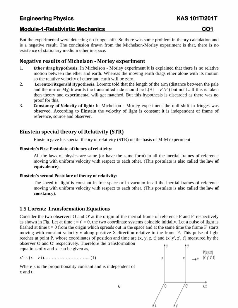
Engineering Physics KAS 101T201T
Module-1-Relativistic Mechanics CO1
6
But the experimental were detecting no fringe shift So there was some problem in theory calculation and
is a negative result The conclusion drawn from the Michelson-Morley experiment is that there is no
existence of stationary medium ether in space
Negative results of Michelson - Morley experiment 1 Ether drag hypothesis In Michelson - Morley experiment it is explained that there is no relative
motion between the ether and earth Whereas the moving earth drags ether alone with its motion
so the relative velocity of ether and earth will be zero
2 Lorentz-Fitzgerald Hypothesis Lorentz told that the length of the arm (distance between the pale
and the mirror M2) towards the transmitted side should be L(radic1 ndash v2c
2) but not L If this is taken
then theory and experimental will get matched But this hypothesis is discarded as there was no
proof for this
3 Constancy of Velocity of light In Michelson - Morley experiment the null shift in fringes was
observed According to Einstein the velocity of light is constant it is independent of frame of
reference source and observer
Einstein special theory of Relativity (STR)
Einstein gave his special theory of relativity (STR) on the basis of M-M experiment
Einsteinrsquos First Postulate of theory of relativity
All the laws of physics are same (or have the same form) in all the inertial frames of reference
moving with uniform velocity with respect to each other (This postulate is also called the law of
equivalence)
Einsteinrsquos second Postulate of theory of relativity
The speed of light is constant in free space or in vacuum in all the inertial frames of reference
moving with uniform velocity with respect to each other (This postulate is also called the law of
constancy)
15 Lorentz Transformation Equations
Consider the two observers O and O at the origin of the inertial frame of reference F and F respectively
as shown in Fig Let at time t = t = 0 the two coordinate systems coincide initially Let a pulse of light is
flashed at time t = 0 from the origin which spreads out in the space and at the same time the frame F starts
moving with constant velocity v along positive X-direction relative to the frame F This pulse of light
reaches at point P whose coordinates of position and time are (x y z t) and (xy z t) measured by the
observer O and O respectively Therefore the transformation
equations of x and x can be given as
x=k (x ndash v t)helliphelliphelliphelliphelliphelliphelliphelliphellip(1)
Where k is the proportionality constant and is independent of
x and t
Engineering Physics KAS 101T201T
Module-1-Relativistic Mechanics CO1
7
The inverse relation can be given as
x=k (x + v t) helliphelliphelliphelliphelliphelliphellip (2)
As t and t are not equal substitute the value of x from Equation (1) in Equation (2)
x=k [k (x ndash vt) + vt] or
=( )
t=
or t=
(
) helliphelliphelliphelliphelliphelliphelliphelliphellip(3)
According to second postulate of special theory of relativity the speed of light c remains constant
Therefore the velocity of pulse of light which spreads out from the common origin observed by observer
O and O should be same
there4 x=c t and x = cthelliphelliphelliphelliphelliphelliphelliphelliphelliphelliphelliphelliphelliphelliphellip(4)
Substitute the values of x and x from Equation (4) in Equation (1) and (2) we get
ct=k (x ndash v t) = k (ct ndash v t) or ct=kt (c ndash v) (5)
and similarly ct=k t (c + v) (6)
Multiplying Equation (5) and (6) we get
c2 t t=k
2t t (c
2 ndash v
2) hence
after solving k=
radic
(7)
Hence equation (7) substitute in equation (1) then Lorentz transformation in position will be
x=
radic
y=y z=z
Calculation of Time equation (7) substitute in equation (3)
t=
(
)
From equation ( 7)
or
then above equation becomes
t=
=
or t= (
)
Engineering Physics KAS 101T201T
Module-1-Relativistic Mechanics CO1
8
Therefore t=
radic
Hence the Lorentz transformation equations becomes
x=
radic
y=y z=z and t=
radic
Under the condition Lorentz transformation equation can be converted in to Galilean
Transformation
x=x -vt y=y z=z and t=t
16 Applications of Lorentz Transformation
161 Length contraction Consider a rod at rest in a moving frame of reference F moving along x-direction with constant velocity
v relative to the fixed frame of reference F as shown in Fig
The observer in the frame F measures the length
of rod AB at any instant of time t This length Lo
measured in the system in which the rod is at rest
is called proper length therefore Lo is given as
Lo= x2- x1 helliphelliphelliphelliphelliphelliphelliphelliphelliphelliphellip(1)
Where x1 and x2 are the coordinates of the two
ends of the rod at any instant At the same time
the length of the rod is measured by an observer
O in his frame say L then
L= x2- x1 helliphelliphelliphelliphelliphelliphelliphelliphelliphelliphellip(2)
Where x1 and x2 are the coordinates of the rod AB
respectively with respect to the frame F According to Lorentz transformation equation
x1=
radic
and x2=
radic
Hence x2- x1=
radic
By using Equations (1) and (2) we can write
Lo=
radic
Engineering Physics KAS 101T201T
Module-1-Relativistic Mechanics CO1
9
Hence L=Lo radic
helliphelliphelliphelliphelliphelliphellip(3)
From this equation Thus the length of the rod is contracted by a factor radic
as measured by observer in
stationary frame F
Special Case
If v ltltlt c then v2c
2 will be negligible in Loradic
and it can be neglected
Then equation (3) becomes L = LO
Percentage of length contraction=
162 Time dilation Let there are two inertial frames of references F and F F is the stationary frame of reference and F is the
moving frame of reference At time t=trsquo=0 that is in the start they are at the same position that is
Observers O and Orsquo coincides After that F frame starts moving with a uniform velocity v along x axis
Let a clock is placed in the frame F The time coordinate of the initial time of the clock will be t1
according to the observer in S and the time coordinate of the final tick (time) will be will be t2 according
to same observer
The time coordinate of the initial time of the clock will be t1 according to the observer in F and the time
coordinate of the final tick (time) will be will be t2 according to same observer
Therefore the time of the object as seen by
observer O in F at the position xrsquo will be
to = trsquo2 ndash trsquo1 helliphelliphelliphelliphelliphelliphelliphelliphelliphelliphelliphellip(1)
The time trsquo is called the proper time of the event
The apparent or dilated time of the same event
from frame S at the same position x will be
t = t2 ndash t1 helliphelliphelliphelliphelliphelliphelliphelliphelliphelliphelliphellip(2)
Now use Lorentz inverse transformation
equations for that is
t1 =
radic
helliphelliphelliphelliphelliphelliphelliphellip (3)
t2 =
radic
helliphelliphelliphelliphelliphelliphelliphellip (3)
Engineering Physics KAS 101T201T
Module-1-Relativistic Mechanics CO1
10
By putting equations (3) and (4) in equation (2) and solving we get
t =
radic
Substitute equation (1) in above equation
t =
radic
This is the relation of the time dilation
Special Case
If v ltltlt c then v2c
2 will be negligible in
radic
and it can be neglected
Then t = to
Experimental evidence The time dilation is real effect can be verified by the following experiment In
1971 NASA conducted one experiment in which JC Hafele as astronomer and RF Keating a physicist
circled the earth twice in a jet plane once from east to west for two days and then from west to east for
two days carrying two cesium-beam atomic clocks capable of measuring time to a nanosecond After the
trip the clocks were compared with identical clocks The clocks on the plane lost 59 10 ns during their
eastward trip and gained 273 7 ns during the westward tripThis results shows that time dilation is real
effect
163 Relativistic Addition of Velocities One of the consequences of the Lorentz transformation equations is the counter-intuitive ldquovelocity
addition theoremrdquo Consider an inertial frame Srsquo moving with uniform velocity v relative to stationary
observer S along the positive direction of X- axis Suppose a particle is also moving along the positive
direction of X-axis If the particle moves through a distance dx in time interval dt in frame S then
velocity of the particle as measured by an observer in this frame is given by
(1)
To an observer in Srsquo frame let the velocity be (by definition)
(2)
Now we have the Lorentz transformation equations
radic(
)
and
radic(
)
(3)
Taking differentials of above equations we get
Engineering Physics KAS 101T201T
Module-1-Relativistic Mechanics CO1
11
and
radic( ) (4)
Using eq (4) in eq(2) we get
(
)
( ) (5)
Or
( ) (6)
This is the the relativistic velocity addition formula If the speeds u and v are small compared to the speed
of light above formula reduces to Newtonian velocity addition formula
Inverse of the formula (6) enables us to find velocity of a particle in S frame if it is given in Srsquo frame
(6)
17 Variation of Mass with Velocity In Newtonian physics mass of an object used to be an absolute entity same in all frames One of the
major unusual consequences of relativity was relativity of mass In the framework of relativity it can be
shown that mass of an object increases with its velocity We have the following equation expressing the
variation of mass with velocity
radic( ) (1)
Where is the mass of the object at rest known as rest mass and is its velocity relative to observer
As it is clear from above equation if in agreement with common experience
Derivation
We use relativistic law of momentum conservation to arrive at eq (1) Consider two inertial frames S and
Srsquo Srsquo moving with respect to S with velocity v along positive X-axis Let two masses and are
moving with velocities ursquo and ndashursquo with respect to moving frame Srsquo
Now let us analyse the collision between two bodies with respect to frame S If u1 and u2
are velocities of two masses with respect to frame S then from velocity addition theorem
and
(2)
Engineering Physics KAS 101T201T
Module-1-Relativistic Mechanics CO1
12
At the time of collision two masses are momentarily at rest relative to frame Srsquo but as seen from frame S
they are still moving with velocity v Since we assume momentum to be conserved even in relativity
theory as seen from S frame
Momentum before collision = momentum after collision
( ) (3)
Substituting the values of u1 and u2 from equation (2) eq(3) becomes
(
) + (
) = ( )
Rearranging the terms
(
) = (
)
( ( )
) ) = (
( )
)
Or ( ( )
) ) = (
( )
)
(4)
Now using set of equations (2) we can find RHS of equation to be equal to
radic
If u2 = 0 ie m2(= m0say) is at rest with respect to S frame above equation reduces to
radic
We could have chosen two masses to be identical In that case m0 will also be the rest mass of So
we can apply above formula to a single with rest mass and moving mass m related by
radic
Engineering Physics KAS 101T201T
Module-1-Relativistic Mechanics CO1
13
This shows that mass of a body increases with its velocity
18 Mass- Energy Equivalence In Newtonian Physics mass and energy are assumed to be quite different entities There is no mechanism
in Newtonian set up how mass and energy can be converted into each other Like many other it is one of
unusual consequences of special relativity that mass and energy are inter-convertible into each other and
hence are equivalent
Einsteinrsquos Mass- energy relation ( ) (Derivation)
Consider a particle of mass m acted upon by a force F in the same direction as its velocity v If F
displaces the particle through distance ds then work done dW is stored as kinetic energy of the particle
dK therefore
(1)
But from Newtonrsquos law
( )
(2)
Using (2) in (1)
Or (3)
Now we have
radic
(
) (4)
Taking the differential
( )(
) (
)
(
)
But ( )
( )
(
)
Or
( )
or ( ) (5)
Using eq (5) in eq (3)
Engineering Physics KAS 101T201T
Module-1-Relativistic Mechanics CO1
14
( )
Let the change in kinetic energy of the particle be K as its mass changes from rest mass to to
effective mass m then
int int
( ) = (
radic
)
This is the relativistic expression for kinetic energy of a particle It says that kinetic energy of a particle is
due to the increase in mass of the particle on account of its relative motion and is equal to the product of
the gain in mass and square of the velocity of light can be regarded as the rest energy of the
particle of rest mass The total energy E of a moving particle is the sum of kinetic energy and its rest
mass energy
( )
Or
This is the celebrated mass- energy equivalence relation This equation is so famous that even common
men identify Einstein with it
Significance This equation represents that energy can neither be created nor be destroyed but it can
change its form
Evidence show its validity
First verification of the was made by Cock-croft and Walton
(70166 amu) (10076 amu) (40026 amu)
Mass defect = (70166 amu+10076 amu) -2x (40028 amu)
=00186 amu
= 00186 x 166 X 10-27
kg
= 00186 x 166 X 10-27
x ( )
=
=( )
( )
=
Engineering Physics KAS 101T201T
Module-1-Relativistic Mechanics CO1
15
( a huge amount of energy release)
19 Relation between Energy and Momentum
a) Relation between total Energy and Momentum
Sconce we know that
radic
Squaring both side
(
)=
=
Science =
substitute in above equation
(
)
= after solving
This is the relation between relativistic total energy and momentum of the particle
b) Relation between Kinetic Energy and Momentum
Science we know that ------------------------(1)
Also we know that
Squaring both side
( ) -----------------------(2)
From equation (1) and (2) we get
= (
)
=
After solving
Engineering Physics KAS 101T201T
Module-1-Relativistic Mechanics CO1
16
radic
Where = kinetic energy
110 Mass-less Particle Zero Rest Mass Particles A particle which has zero rest mass( ) is called massless particle
We have the energy-momentum relation
radic ( ) (1)
For a massless particle
Therefore or (2)
But therefore
Which implies
This says that a massless particles always move with the speed of light Energy and momentum of a
massless particle is given by equation (2) Massless particles can exist only as long as the move at the
speed of light Examples are photon neutrinos and theoretically predicted gravitons
Numerical Problems
Question 1 Show that the distance between any two points in two inertial frame is invariant under
Galilean transformation
Answer Consider two frame of reference S and frame moving with constant velocity relative
to frame S in positive X-direction
Point A and B placed in frame S and their co-ordinate relative O are ( ) and ( )
After time the coordinate of A and B relative to observer from frame will be ( )
and( )
Using Galilean Transformation
and
and
Engineering Physics KAS 101T201T
Module-1-Relativistic Mechanics CO1
17
Now distance between two points from frame will be
=radic( ) ( ) ( )
Substitute all values then
=radic( ) ( ) ( )
After simplification
=radic( ) ( ) ( ) ie
=
This show that distance between two points is invariant under Galilean Transformation
Question 2 Show that the relativistic form of Newtonrsquos second law when is parallel to
=
(
)
Answer Science we know that
=
(
radic
)=[ ( (
)
)]
= [
(
)
(
) (
)
(
)]
=
[(
)
(
)
]
=
(
)
+
=
(
)
it is relativistic Newtonrsquos second law
Engineering Physics KAS 101T201T
Module-1-Relativistic Mechanics CO1
18
If then
=
= (because at )
So it can also be written as =
Question 3 A particle of rest mass moves with speed
radic Calculate its mass momentum total energy
and kinetic energy
Answer Science we know that
radic
=
radic
= radic =141
The momentum of the particle is given by
radic =
Total energy of the particle
=
Kinetic energy
= -
=
Question 4 A man weight 50 kg on the earth when he is in a rocket ship in flight his mass is 505 kg ass
measured by an observer on earth What is the speed of rocket
Answer Given that
=50 kg
radic(
)
substitute all values and after solving
ms
Question 5 Compute the mass m and speed of an electron having kinetic energy Given rest
mass of electron
Answer Given that
Engineering Physics KAS 101T201T
Module-1-Relativistic Mechanics CO1
19
Kinetic energy( ) ( )
Kinetic energy( ) ( )
hence
substitute all values and after solving
=
Using the relation
radic(
)
where = and
Then after solving
Question 6 Calculate the amount of work to be done to increase the speed of an electron from 06c to
08c Given that rest mass energy of electron ( )
Answer
Kinetic energy( ) ( ) =(
radic(
)
)
Where
For speed 06c For speed 08c
=(
radic( ( )
)
) =(
radic( ( )
)
)
= =
Hence The amount of work to be done(electron increase the speed 06c to 08c)=
=
Engineering Physics KAS 101T201T
Module-2-Electromagnetic Field Theory CO2
20
21 Continuity equation for current density Statement Equation of continuity represents the law of conservation of charge The charge flowing out
through a closed surface from some volume is equal to the rate of decrease of charge within the volume
hellip (1)
Where I is current flowing out through the surface of a volume and
is the rate of decrease of charge
within the volume
Again we know ∯ and q= intintintρdv
where J is the Conduction current density an ρ is the volume charge density
Substituting the expression of I and q in equation (1)
∯ ∭
hellip (2)
Now applying Gaussrsquos Divergence Theorem to LHS of above equation
∭ ∭
As the two volume integrals are equal so their integrands are also equal
Thus
This is continuity equation for time varying fields
Equation of Continuity for Steady Currents As ρ does not vary with time for steady currents that is
So
This is the continuity equation for steady currents
Engineering Physics KAS 101T201T
Module-2-Electromagnetic Field Theory CO2
21
22 Differential form of Maxwellrsquos equations
221 First equation (Gauss Law of Electrostatic)
Gauss law of electrostatic states that the total electric flux E coming out from a closed surface is equal to
1ε0 times the net charge enclosed by the surface ie ∯
∯ =intintintρdv hellip (1)
Applying Gaussrsquos Divergence theorem to change LHS of equation (1) ∯ =intv (nablaD) dv
Using this equation in equation (1) we will get
intintint (nablaD)dv=intintintρdv
As two volume integrals are equal so their integrands are also equal
Thus nablaD=ρ hellip (2)
The above equation is the Differential form of Maxwellrsquos first equation
222 Second equation(Gauss Law of Magnetostatic)
Gauss law of magnetostatic states that the total magnetic flux φm coming out through surface of a volume
is always equal to zero
φm=∯ hellip(3)
Applying Gaussrsquos Divergence theorem ∯ =intintint(nablaB)dv
Putting this in equation (3) intintint (nablaB)dv =0
Thus nablaB=0 hellip(4)
This equation (4) is differential form of Maxwellrsquos second equation
223 Third Equation(Faradayrsquos Law of Electromagnetic Induction)
1 It states that if there is a change of magnetic flux linked with a circuit then electromotive force (emf) is
induced in the circuit This induced emf lasts as long as the change in magnetic flux continues
Engineering Physics KAS 101T201T
Module-2-Electromagnetic Field Theory CO2
22
2 The magnitude of induced emf is equal to the rate of change of magnetic flux linked with the circuit
Therefore induced emf
hellip(5)
Where φm= intintBds hellip(6)
Here negative sign indicates the induced emf set up a current in such a direction that the magnetic effect
produced by it opposes the cause producing it
Again we know emf is the closed line integral of the non-conservative electric field generated by the
battery
That is emf=∮ hellip(7)
Putting equations (6) and (7) in equation (5) we get
∮ = ndash intint
ds hellip(8)
Using Stokersquos theorem to the LHS of equations (8) ∮ = intint (nabla x E)ds
Substituting above equation in equation (8) we get
intint (nabla x E)dS = -intint
ds
Two surface integral are equal only when their integrands are equal
Thus nabla x E = ndash
hellip(9)
This is the differential form of Maxwellrsquos 3rd
equation
224 Forth Equation (Modified Amperersquos Circuital Law)
To come to the Maxwellrsquos 4th
equation let us first discuss Amperersquos circuital law
Amperersquos circuital law This law states that the line integral of the magnetic field H around any closed
path or circuit is equal to the current enclosed by that path
That is ∮ =I
Engineering Physics KAS 101T201T
Module-2-Electromagnetic Field Theory CO2
23
If J is the current density then I=intintJds
This implies that ∮ =intintJds hellip(10)
Applying Stokersquos theorem to LHS of above equation ∮ =intint(nablaxH)ds
Substituting above equation in equation (10) we will get intint(nablaxH)ds =intintJds
Two surface integrals are equal only if their integrands are equal
Thus nablax H=J hellip(11)
This is the differential form of Amperersquos circuital Law for steady currents
Now taking divergence on both side of equation (10) nabla(nablaxH)= nablaJ
As divergence of the curl of a vector is always zero therefore nabla(nablaxH)=0
It means nablaJ=0
Now this is continuity equation for steady current but not for time varying fields as equation of
continuity for time varying fields is
So Amperersquos circuital law is incomplete valid only for steady state current This is the reason that led
Maxwell to modify Amperersquos circuital law
Modification of Amperersquos circuital law Maxwell modified Amperersquos law by giving the concept of
displacement current and displacement current density for time varying fields
He considered that equation (10) for time varying fields can be written as nablaxH=J + Jd hellip (12)
By taking divergence on both side of equation (12) we will get nabla (nabla xH)= nablaJ+ nablaJd
As the divergence of curl of a vector is always zero therefore nabla (nabla xH)= 0
So nabla (J+Jd)=0 Or nabla J= -nablaJd
But from equation of continuity for time varying fields
Engineering Physics KAS 101T201T
Module-2-Electromagnetic Field Theory CO2
24
From the above two equations of j we get
nabla Jd = ( )
hellip (13)
As from Maxwellrsquos first equation nablaD=ρ
Now from equation (13) we can write
Using the above equation in equation (12) we get
nabla x H=J +
hellip(14)
Here
=Displacement current density
The equation (14) is the Differential form of Maxwellrsquos fourth equation or Modified Amperersquos circuital
law
23 Integral form of Maxwellrsquos equations
231 First Equation
Gauss law of electrostatic states that the total electric flux E coming out from a closed surface is
equal to 1ε0 times the net charge enclosed by the surface ie
∯ hellip(1)
Let ρ is the volume charge density distributed over a volume V
Therefore q=int ρ dv
So ∯
hellip(2)
This equation is the integral form of Maxwellrsquos first equation or Gaussrsquos law in electrostatics
232 Second equation
Gauss law of magnetostatic states that the total magnetic flux φm coming out through surface of a volume
is always equal to zero ie
φm=∯ hellip(3)
Engineering Physics KAS 101T201T
Module-2-Electromagnetic Field Theory CO2
25
The above equation is the intergal form of Maxwellrsquos second equation
The above equation also suggest that magnetic monopole does not exist
233 Third Equation
1 It states that if there is a change of magnetic flux linked with a circuit then electromotive force (emf) is
induced in the circuit This induced emf lasts as long as the change in magnetic flux continues
2 The magnitude of induced emf is equal to the rate of change of magnetic flux linked with the circuit
Therefore induced emf
hellip(4)
Where φm= intintBds hellip(5)
Here negative sign indicates the induced emf set up a current in such a direction that the magnetic effect
produced by it opposes the cause producing it
Again we know emf is the closed line integral of the non-conservative electric field generated by the
battery
That is emf=∮ hellip(6)
Using equations (5) and (6) in equation (4) we get
∮ = ndash intint
ds hellip(7)
The above equation is the integral form of Maxwellrsquos third Equation or Faradayrsquos law of
electromagnetic induction
234 Fourth equation
The line integration of the magnetic field H around a closed path or circuit is equal to the conductions
current plus the time derivative of electric displacement through the surface bounded by the closed path
ie
∮ =∬(
) (8)
The above equation is the integral form of Maxwellrsquos fourth equation
Engineering Physics KAS 101T201T
Module-2-Electromagnetic Field Theory CO2
26
25 Displacement Current
According to Maxwell not only conduction current produces magnetic field but also time varying electric
field produces magnetic field This means that a changing electric field is equivalent to a current which
flows as long as electric filed is changing This is current only in the sense that it produces same magnetic
effect as conduction current does there is no actual flow of electron
If E is the electric field developed between the plates of surface area A Then the displacement current is
given by
26 Electromagnetic wave Equation in Free Space
Now in free space there is no charge so charge density ρ=0 and current will also be zero Thus current
density J is also equal to zero
Hence Maxwellrsquos equation in free space is given by
hellip(1) where ( )
hellip(2)
hellip(3) where ( )
hellip(4) where ( )
261 Maxwellrsquos Electromagnetic wave Equation in Free Space for the field vector E
we take curl on both side of Maxwellrsquos 3rd
equation represented in equation (3)
( )
( ) ( )
[(using vector identity ( ) ( ) ]
Now from equation (1) and (4) in the above equation
Engineering Physics KAS 101T201T
Module-2-Electromagnetic Field Theory CO2
27
(
)
Or
hellip(5)
Similarly we can find an equation for the field vector B when we take the Maxwellrsquos 4th
and repeat the
process of field vector E
hellip(6)
Equation (5) and (6) is the guiding equation for field vector E and B respectively in free space
Thus we can see that time varying electric field produces magnetic field and time varying magnetic field
produces electric filed and follow the above guiding equation Comparing the above equation with the
standard wave equation
-------(7)
Compare equation (6) and (7) we get
radic radic
radic
Because
Hence = c
Hence this field vectors propagates in free space with the speed of light So from here Maxwell
concluded that light is an electromagnetic wave
27 Electromagnetic wave Equation in non-conducting medium
Now in non-conducting medium there is no free charge so current density J and total charge inside the
material is zero so charge density ρ is also equal to zero Maxwellrsquos equation in a non-conducting
medium of permittivity and permeability is reduces to
Engineering Physics KAS 101T201T
Module-2-Electromagnetic Field Theory CO2
28
hellip(1) where ( )
hellip(2)
hellip(3) where ( )
hellip(4) where ( )
271 Maxwellrsquos Electromagnetic wave Equation in Free Space for the field vector E
we take curl on both side of Maxwellrsquos 3rd
equation represented in equation (3)
( )
( ) ( )
[(using vector identity ( ) ( ) ]
Now using equation (1) and (4) in the above equation
(
)
Or
hellip(5)
Similarly we can find an equation for the field vector B when we take the Maxwellrsquos 4th
and repeat the
process of field vector E
hellip(6)
Equation (5) and (6) is the guiding equation for field vector E and B respectively in non-conducting
medium
Comparing the above equation with the standard wave equation
----------(7)
Engineering Physics KAS 101T201T
Module-2-Electromagnetic Field Theory CO2
29
we can see that this field vectors propagate in non-conducting medium with a speed
radic
radic
radic As 119888
radic
For non-magnetic medium 119903=1
So
radic
here radic 119903 119899 is the refractive index of the medium
Hence electromagnetic wave propagate in non-conducting medium with a speed
times the speed of
electromagnetic wave in free space
28 Transverse nature of electromagnetic wave
Science we know that the plane electromagnetic wave equation are
---(1)
---(2)
Solution of these wave equation considering the propagation of the wave in any arbitrary direction of
three dimensional space is given by
( 119903 ) (3)
( 119903 ) hellip(4)
Where E0 and B0 are the amplitudes of electric and magnetic field respectively and is propagation vector
given by = 2πλ = 2πνc = ωc
Now Maxwellrsquos first and second equation in free space is
nabla =0 hellip(5)
nabla hellip(6)
Engineering Physics KAS 101T201T
Module-2-Electromagnetic Field Theory CO2
30
Where nabla
and = 119910 119911
Putting the above expressions in L H S of equation (5)
nabla = (
) ( 119903 ) ------ (7)
Where k ky kz
and 119903 = y
So 119903 = k yky kz
Thus equation (7) can be written as
= (
)( 119910 119911
) exp ί( k yky kz )- +
=
[ exp ί ( k yky k
z )
- +]+
[ 119910exp ί ( k yky k
z )
- +]+
[ 119911
exp ί ( k yky kz )
- +]
=(ί k ) exp ί ( k yky kz )
- + +(ίky) 119910exp ί ( k yky k
z) - + +(ίk
z )
119911 exp ί ( k yky k
z )
- +
= ί[ k + 119910ky+ 119911 k
z] exp ί ( k yky k
z) - +
= ί[( k ky kz )( 119910 119911
)] exp ί ( k yky k
z )
- +
= ί( )exp(( 119903 )= ί
= ί using equation (3)
Now putting the value of in equation (5)
= ί
Or helliphellip (8)
Similarly putting equation (4) in equation (6) we will get hellip(9)
Equation (8) amp (9) suggest that electric and magnetic field vectors are perpendicular to propagation
vector So we can say that electromagnetic waves are transverse in nature
Again using Maxwellrsquos 3rd
and 4th
equations in free space are
hellip(10)
Engineering Physics KAS 101T201T
Module-2-Electromagnetic Field Theory CO2
31
hellip(11)
Now if we put the expression of from equation (3) in above Maxwellrsquos equation (equation No 10) then
we can write
ί [ ] =
( 119903 )]
= -(- ) ( 119903 )
= hellip(12)
Similarly putting the expression of from equation (4) in equation (12) we will get
= - -----(13)
From equation (12) we can say magnetic field vector is perpendicular to both amp and from (13) we
can say Electric field vector is perpendicular to both Thus electric field vector magnetic field
vector and propagation vector are mutually perpendicular to each other
Characteristic Impedance
As amp are perpendicular to each other and amp are mutually perpendicular so from
equation (12)
=
Or
Or
=
νλ = c
Thus
= c
Or
= micro
0 c and 119888
radic
Or
=
radic
= radic
= 37672 Ω
The quantity
= Z
0 = 37672Ω is known as characteristic Impedance or Intrinsic Impedance of free
space
Engineering Physics KAS 101T201T
Module-2-Electromagnetic Field Theory CO2
32
29 Energy in an electromagnetic field
The Energy of electromagnetic Wave is the sum of electric (E) and magnetic (B) field energy
The electric energy per unit volume is given by UE
The magnetic energy per unit volume is given by UB
So the total energy per unit volume in electromagnetic wave is
U =
As
and
radic So U =
+
=
+
= Ɛ0E
2
Therefore energy per unit volume in electromagnetic wave is U = Ɛ0E2
210 Skin Depth
Skin depth or depth of penetration is defined as the depth in which the strength of electric field associated
with electromagnetic wave reduces to 1e times of its initial value The figure below shows the variation
of field vector E with distance of electromagnetic wave inside a conducting medium and the value of skin
depth inside a good conductor is given by radic
Here is the conductivity of the medium and
is angular frequency of the electromagnetic wave
Engineering Physics KAS 101T201T
Module-2-Electromagnetic Field Theory CO2
33
211 Poynting vector and Poynting Theorem
Poynting vector When electromagnetic wave propagates through space it carries energy with it The
amount of energy passing through unit area in the perpendicular to direction of propagation of the
electromagnetic wave per second is given by S = E x H
This quantity S is called Poynting vector E electric field vector and H is magnetic field vector of the
electromagnetic wave The direction of S is perpendicular to E and H and in the direction of vector E x H
Theorem Consider Maxwellrsquos fourth equation (Modified Amperersquos Circuital Law) that is
nabla x H = J + ε dEdt
or J = (nabla x H) ndash ε dEdt
The above equation has the dimensions of current density Now to convert the dimensions into rate of
energy flow per unit volume take dot product of both sides of above equation by E that is
E J = E (nabla x H) ndash εE dEdt (1)
Now using vector Identity
nabla (E x H) = H (nabla x E) ndash E (nabla x H)
or E (nabla x H) = H (nabla x E) ndash nabla ( E x H )
By substituting value of E (del x H) in equation (1) we get
Engineering Physics KAS 101T201T
Module-2-Electromagnetic Field Theory CO2
34
E J =H(nabla x E) ndash nabla(E x H) ndash εEdEdt (2)
Also from Maxwellrsquos third equation (Faradayrsquos law of electromagnetic induction)
nabla x E = μdHdt
By substituting value of nabla x E in equation (2) we get
E J =μHdHdt ndash εE dEdt ndash nabla (E x H) (3)
We can write
H dHdt = 12 dH2dt (4a)
E dEdt = 12 dE2dt (4b)
By substituting equations 4a and 4b in equation 3 we get
E J = -μ2 dH2dt ndash ε2 dE
2dt ndash nabla (E x H)
E J = -d(μH22 + εE
2 2)dt ndash nabla (E x H)
By taking volume integral on both sides we get
intintintE JdV = -d[intintint (μH22 + εE
2 2)dV]dt ndash intintint nabla (E H) dV (5)
Applying Gaussrsquos Divergence theorem to second term of RHS to change volume integral into surface
integral that is
intintint nabla(E H) dV = ∯( )
Substitute above equation in equation (5)
intintintE JdV = -d[intintint (μH22 + εE
2 2)dV]dt ndash ∯ (6)
Engineering Physics KAS 101T201T
Module-2-Electromagnetic Field Theory CO2
35
or ∯ = -intintint[d(μH22 + εE
2 2)dt] dV ndashintintintE J dV
Interpretation of above equation
LHS Term
∯ rarr It represents the rate of outward flow of energy through the surface of a volume V and
the integral is over the closed surface surrounding the volume This rate of outward flow of power from a
volume V is represented by
∯ ∯
where Poynting vector S = E H
Inward flow of power is represented by ∯ ∯
RHS First Term
-intintint[d(μH22 + εE
2 2)dt] dV rarr If the energy is flowing out of the region there must be a
corresponding decrease of electromagnetic energy So here negative sign indicates decrease
Electromagnetic energy is the sum of magnetic energy μH22 and electric energy εE
2 2 So first term of
RHS represents rate of decrease of stored electromagnetic energy
RHS Second Term
ndashintintintE J dV rarrTotal ohmic power dissipated within the volume
So from the law of conservation of energy equation (6) can be written in words as
Rate of energy dissipation in volume V = Rate at which stored electromagnetic energy is decreasing in V
+ Inward rate of flow of energy through the surface of the volume
212 Radiation Pressure
The electromagnetic waves exert a ldquoRadiation Pressurerdquo on a surface due to absorption and reflection of
the electromagnetic wave An object absorbing an electromagnetic wave would experience a force in the
direction of propagation of the wave During these processes momentum is exchanged between the
surface and the electromagnetic wave
Engineering Physics KAS 101T201T
Module-2-Electromagnetic Field Theory CO2
36
Consider an em wave of average energy density ltugt and average poynting vector ltSgt be incident
normally on a surface then the radiation pressure P exerted by em waves on this surface is
hellip (1)
where ltFgt is the average force exerted by the em waves
Now using Newtonrsquos Second Law
hellip(2)
Where ltPgt is the momentum of incident em waves
For electromagnetic wave we know that
hellip(3)
Putting equation ( 3 ) in ( 2 )
hellip(4)
Since S= PowerArea and Power = EnergyTime
Therefore S=
So we can write
hellip(5)
Now using equation ( 5 ) in ( 4 )
119888 hellip(6)
Using equation ( 6 ) in ( 1 ) radiation pressure due to absorption of electromagnetic wave is
Engineering Physics KAS 101T201T
Unit-III-Quantum Mechanics CO3
BLACKBODY RADIATION SPECTRUM
A blackbody is an object that absorbs all of the radiation that it receives (that is it does not reflect any light nor does it allow any light to pass through it and out the other side) The energy that the blackbody absorbs heats it up and then it will emit its own radiation The only parameter that determines how much light the blackbody gives off and at what wavelengths is its temperature There is no object that is an ideal blackbody but many objects (stars included) behave approximately like blackbodies Other common examples are the filament in an incandescent light bulb or the burner element on an electric stove As you increase the setting on the stove from low to high you can observe it produce blackbody radiation the element will go from nearly black to glowing red hot
Plot of the spectrum of a blackbody with different temperatures
The spectrum of a blackbody is continuous (it gives off some light at all wavelengths) and it has a peak at a specific wavelength The peak of the blackbody curve in a spectrum moves to shorter wavelengths for hotter objects
Rayleigh-Jeans radiation law
The Rayleigh-Jeans Radiation Law was a useful but not completely successful attempt at establishing the functional form of the spectra of thermal radiation The energy density uν per unit frequency interval at a frequency ν is according to the The Rayleigh-Jeans Radiation
(1) dνuν = c38πν kT2
where k is Boltzmanns constant T is the absolute temperature of the radiating body and c is the speed of light in a vacuum This formula fits the empirical measurements for low frequencies but fails increasingly for higher frequencies The failure of the formula to match the new data was called the ultraviolet catastrophe The significance of this inadequate so-called law is that it provides an asymptotic condition which other proposed formulas such as Plancks need to satisfy It gives a value to an otherwise arbitrary constant in Plancks thermal radiation formula
1
user
Textbox
37
Engineering Physics KAS 101T201T
Unit-III-Quantum Mechanics CO3
Stefanrsquos Law
The spectrum of radiation emitted by a solid material is a continuous spectrum unlike the line spectrum emitted by the same material in gaseous form The peak frequency of the emitted spectrum increases with the temperature of the solid body as does the total power radiated
Definition According to the Stefan-Boltzmann law the total power radiated by an ideal emitter (perfect blackbody) is proportional to the fourth power of the absolute temperature
P = AσT4
Where P = total power radiated from the blackbody
A = surface area of the blackbody σ = Stefan-Boltzmann constant
T = Absolute temperature of the blackbody To generalize
P = 120692AσT4
Where 120692 is the emissivity And
120692 = 1 for black body 120692 lt 1 for grey bodies (not perfect blackbody
Wienrsquos Displacement Law
When the temperature of a blackbody radiator increases the overall radiated energy increases and the peak of the radiation curve moves to shorter wavelengths When the maximum is evaluated from the Planck radiation formula the product of the peak wavelength and the temperature is found to be a constant
λmT = 2898 x 10-3mK (2)
This relationship is called Wiens displacement law and is useful for the determining the temperatures of hot radiant objects such as stars and indeed for a determination of the temperature of any radiant object whose temperature is far above that of its surroundings
Refhttphyperphysicsphy-astrgsueduhbasewienhtml
2
user
Textbox
38
Engineering Physics KAS 101T201T
Unit-III-Quantum Mechanics CO3
Wienrsquos Distribution law
William Wien used thermodynamics to show that the spectral energy density of a blackbody between the wavelength range 120524 and 120524+d120524 is given by
E120582119889120582 = 119860 119891(120582119931) 119889120582 hellip (1)
1205825
Wien found using the Maxwell-Boltzmann distribution law for the speed of atoms (or molecules) in a gas that the form of the function f (120524T) was
119891(120582119931) = 119942 -120572 120582119931 hellip (2) And therefore
E120582119889120582 = 119860 120582-5 119942 -120572 120582119931119889120582 hellip (3) Where A and 120514 are constants to be determined Equation (3) is known as Wienrsquos Distribution Law Assumption of Quantum Theory of Radiation
The distribution of energy in the spectrum of radiations of a hot body cannot be explained by applying the classical concepts of physics Max Planck gave an explanation to this observation by his Quantum Theory of Radiation His theory says
a) The radiant energy is always in the form of tiny bundles of light called quanta ie the energy is absorbed or emitted discontinuously
b) Each quantum has some definite energy E=hν which depends upon the frequency (ν) of the radiations where h = Planckrsquos constant = 6626 x10-34Js
c) The energy emitted or absorbed by a body is always a whole multiple of a quantum ie nhνThis concept is known as quantization of energy
Planckrsquos Law(or Planckrsquos Radiation Law)
Plancks radiation law is derived by assuming that each radiation mode can be described by a quantized harmonic oscillator with energy En = nhν
Let N0 be the number of oscillators with zero energy ie E0 (in the so-called ground-state) then the numbers in the 1st 2nd 3rd etc levels (N1 N2 N3hellip) are given by
N exp N 1 = 0 ( kTminusE1 ) N exp N exp N 2 = 0 ( kT
minusE2 )N 3 = 0 ( kTminusE3 )
3
user
Textbox
39
Engineering Physics KAS 101T201T
Unit-III-Quantum Mechanics CO3
But since En = nhν
N exp N 1 = 0 ( kTminushν) N exp N exp N 2 = 0 ( kT
minus2hν) N 3 = 0 ( kTminus3hν)
The total number of oscillators N = N0 + N1 + N2 + N3helliphelliphelliphelliphellip
The total energy E = + + +hellipνN xp h 0 exp e ( kTminushν) exp 2hνN 0 ( kT
minus2hν) exp 3hνN 0 ( kTminus3hν)
The avg energy lt E gt = EN
lt E gt = N 1+exp xp ( ) +exp xp ( ) +hellip0[ e kTminushν e kT
minus2hν ]hνN exp xp ( ) + ( ) + ( ) +hellip0[ e kT
minushνkT
minus2hνkT
minus3hν ]
lt E gt = hν xp ( ) exp e kTminushν
1minusexp xp ( ) [ e kTminushν ]
(4)lt E gt = hν exp xp ( )minus1 [ e hν
kT ]
According to Rayleigh-Jeans law using classical physics the energy density uνper frequency interval was given by
(5)dνuν = c38πν kT 2
where kT was the energy of each mode of the electromagnetic radiation We need to replace the kT in this equation with the average energy for the harmonic oscillators that we have just derived above So we re-write the energy density as
(6)dνuν = c38πν2 hν
exp xp ( )minus1 [ e hνkT ]
Comparison of Rayleigh Jeans Wienrsquos amp Planckrsquos Radiation Laws for the blackbody radiation spectrum
4
user
Textbox
40
Engineering Physics KAS 101T201T
Unit-III-Quantum Mechanics CO3
WAVE PARTICLE DUALITY
In physics and chemistry wave-particle duality holds that light and matter exhibit properties of both waves and of particlesA central concept of quantum mechanics duality addresses the inadequacy of conventional concepts like particle and wave to meaningfully describe the behaviour of quantum objects
Publicized early in the debate about whether light was composed of particles or waves a wave-particle dual nature soon was found to be characteristic of electrons as well The evidence for the description of light as waves was well established at the turn of the century when the photoelectric effect introduced firm evidence of a particle nature of light as well On the other hand the particle properties of electron was well documented when the DeBroglie hypothesis and the subsequent experiments by Davisson and Germer established the wave nature of the electron
Refhttphyperphysicsphy-astrgsueduhbasemod1html
De Broglie Matter Waves
De Broglie Hypothesis
In 1924 Lewis de-Broglie proposed that matter has dual characteristic just like radiation His concept about the dual nature of matter was based on the following observations-
(a) The whole universe is composed of matter and electromagnetic radiations Since both are forms of energy so can be transformed into each other
(b) The matter loves symmetry As the radiation has dual nature matter should also possess dual character
5
user
Textbox
41
Engineering Physics KAS 101T201T
Unit-III-Quantum Mechanics CO3
According to the de Broglie concept of matter waves the matter has dual nature It means when the matter is moving it shows the wave properties (like interference diffraction etc) are associated with it and when it is in the state of rest then it shows particle properties Thus the matter has dual nature The waves associated with moving particles are matter waves or de-Broglie waves
(7)λ = hmv
where λ = de Broglie wavelength associated with the particle h = Planckrsquos constant m = relativistic mass of the particle and v = velocity of the particle
Phase velocityGroup Velocity (MATTER WAVES) The phase velocity of a wave is the rate at which the phase of the wave propagates in space This is the velocity at which the phase of any one frequency component of the wave travels Let P be a phase point located on a travelling wave represented by the equation Asin(kx t) y = minus ω where πλ is the wave number k = 2 ω πν is the angular f requency = 2
then the phase velocity is given by = vp λ ν = k
ω (8) Also and E=mc2ν = h
E (9) and λ = p
h v p = m (10)
Substituting (9) and (10) in (8) we obtain = = vp pE
vctimesc
The velocity of the phase point will be the same as the wave velocity As already mentioned v = velocity of the particle associated with the waveTherefore For Photon v = c so in vacuum vp = c For other particles v lt c but vpgt c which has no physical significance For a physically significant representation of matter waves we require a wave packet to be associated with the moving particle(or body)
6
user
Textbox
42
Engineering Physics KAS 101T201T
Unit-III-Quantum Mechanics CO3
The velocity of the wave packet is called Group Velocity 119907119892 = 119889120596 = 119889119864 (11)
119889119896 119889119901
BORN INTERPRETATION OF THE WAVE FUNCTION AND ITS SIGNIFICANCE Matter waves are represented by a complex function Ψ (xt) which is called a wave function The wave function is not directly associated with any physical quantity but the square of the wave function represents the probability density in a given region The wave function should satisfy the following conditions (i) Ψ should be finite (ii)Ψ should be single valued (iii) Ψ and its first derivative should be continuous (iv) Ψ should be normalizable
2 dV = 1 where V = volume in which the particle is expected to be foundint
VΨ| |
SCHRODINGERrsquoS WAVE EQUATION
TIME INDEPENDENT SCHRODINGERrsquoS EQUATION
The classical wave equation that describes any type of wave motion can be given as
= partx2part y(xt) 2 1
v2 partt2part y(xt)2
Where y is a variable quantity that propagates in lsquox lsquo direction with a velocity lsquovrsquo Matter waves should also satisfy a similar equation and we can write the equation for matter waves as
= (17)partx2part ψ(xt) 2 1
v2 partt2part ψ(xt)2
We can eliminate the time dependence from the above equation by assuming a suitable form of the wave function and making appropriate substitutions
7
user
Textbox
43
Engineering Physics KAS 101T201T
Unit-III-Quantum Mechanics CO3
(x ) ψ (x)e ψ t = 0minusiωt (18)
Differentiate eqn (18) wrt lsquoxrsquo successively to obtain
= (19)partx2part ψ(xt) 2
partx2part ψ (x) 2
0 eminusiωt
Differentiate eqn (18) wrt lsquotrsquo successively to obtain
= (20)partt2part ψ(xt) 2
minus ω) ψ (x)( i 20 eminusiωt
Substituting (19) and (20) in equation (17)
= = (21)partx2part ψ (x) 2
0 minus v2ω2 (x) ψ0 ψ (x) minus k2
0
= 0partx2part ψ (x) 2
0 ψ (x) + k20 (22)
Now we know the total energy lsquoE of the particle is the sum of its kinetic energy and potential energy
ie + V rArr (23)E = 2mp2
2m(E ) p2 = minus V
Also and rArr (24)k = λ2π λ = p
h k2 = h24π p2 2
Substituting (23) in (24) in then substituting result in (22) we get
= 0partx2part ψ (x) 2
0 ψ (x)+ h28mπ (EminusV )2
0 (25)
Replacing Ψ0(x )by Ψ (x) in eqn(vii) we obtain the Schrodingerrsquos time independent wave equation in one dimension as
= 0partx2part ψ(x) 2
ψ(x)+ h28mπ (EminusV )2
(26)
The above equation can be solved for different cases to obtain the allowed values of energy and the allowed wave functions
TIME DEPENDENT SCHRODINGERrsquoS EQUATION
In the discussion of the particle in an infinite potential well it was observed that the wave function of a particle of fixed energy E could most naturally be written as a linear combination of wave functions of the form
(x ) Ae ψ t = i(kxminusωt)
8
user
Textbox
44
Engineering Physics KAS 101T201T
Unit-III-Quantum Mechanics CO3
representing a wave travelling in the positive x direction and a corresponding wave travelling in the opposite direction so giving rise to a standing wave this being necessary in order to satisfy the boundary conditions This corresponds intuitively to our classical notion of a particle bouncing back and forth between the walls of the potential well which suggests that we adopt the wave function above as being the appropriate wave function for a free particle of momentum p = ℏk and energy E = ℏω With this in mind we can then note that
(27)partx2part ψ(x) 2
ψ(x) = minus k2
which can be written using = (28)E = p2
2m 2mℏ k2 2
From (28) and (27) we get
= (29) 2mminus ℏ 2
partx2 part ψ(x) 2
2m p ψ(x) 2
Similarly
= parttpartψ ωψ minus i (30)
which can be written using ω E = ℏ (31)
From (30) and (31)
= ℏ i parttpartψ ψ E (32)
We now generalize this to the situation in which there is both a kinetic energy and a potential energy present then E = p22m + V (x) so that
+ ψ E = 2mp ψ 2
(x)ψ V (33)
where Ψ is now the wave function of a particle moving in the presence of a potential V (x) But if we assume that the results above still apply in this case then we have by substituting (29) and (32) in (33)
+ 2mminus ℏ2
partx2 part ψ(x) 2
(x)ψ ℏ V = i parttpartψ (34)
which is the famous time dependent Schrodinger wave equation It is setting up and solving this equation then analyzing the physical contents of its solutions that form the basis of that branch of quantum mechanics known as wave mechanicsEven though this equation does not look like the familiar wave equation that describes for instance waves on a stretched string it is nevertheless referred to as a lsquowave equationrsquoas it can have solutions that represent waves propagating through space We have seen an example of this the harmonic wave function for a free particle of energy E and momentum p ieis a solution of this equation with as appropriate for a free particle V (x) = 0 But this equation can have distinctly non-wave like solutions whose form depends amongst other things on the nature of the potential V (x) experienced by the particle
9
user
Textbox
45
Engineering Physics KAS 101T201T
Unit-III-Quantum Mechanics CO3
(x ) Ae ψ t = i(pxminusEt)ℏ
In general the solutions to the time dependent Schrodinger equation will describe the dynamical behaviour of the particle in some sense similar to the way that Newtonrsquos equation F = ma describes the dynamics of a particle in classical physics However there is an important difference By solving Newtonrsquos equation we can determine the position of a particle as a function of time whereas by solving Schrodingerrsquos equation what we get is a wave function Ψ(x t) which tells us (after we square the wave function) how the probability of finding the particle in some region in space varies as a function of time
PARTICLE IN AN INFINITE POTENTIAL BOX
Consider a particle of mass lsquomrsquo confined to a one dimensional potential well of dimension lsquoLrsquo The potential energy V = infin at x=0 and x= L and V = 0 for 0le x le L The walls are perfectly rigid and the probability of finding the particle is zero at the wallsHence the boundary conditions are Ψ(x ) = 0 at x=0 and x= L The one dimensional time independent wave equation is
ψ(x) 0partx2part ψ(x) 2
+ℏ2
2m(EminusV ) = (35)
We can substitute V=0 since the particle is free to move inside the potential well
ψ(x) 0partx 2part ψ(x) 2
+ℏ2
2mE = (36)
Let and the wave equation (36) can be written isℏ2
2mE
= k2
ψ(x) 0 partx2part ψ(x) 2
+ k2 =
The above equation represents simple harmonic motion and the general solution is
(x) A sin kx B cos kx ψ = +
Applying the condition we get rArr B=0(x) at x ψ = 0 = 0 0 B 0 = A +
Applying the condition we get rArr k=(n120587) L(x) at x ψ = 0 = L sin kL 0 = A
where n = 0123hellip positive integer
Eigen values of energy
= = En = 2mk ℏ 2 2 n π h2 2 2
8π mL2 2n h2 2
8mL2 (37)
10
user
Textbox
46
Engineering Physics KAS 101T201T
Unit-III-Quantum Mechanics CO3
lsquonrsquo is the quantum number corresponding to a given energy level n=1 corresponds to the ground state n=2 corresponds to the first excited state and so on
Eigen functions
The allowed wavefunctions are
(x) ψn = A in (nπxL) s (38)
The constant A can be evaluated from normalization condition
sin (nπxL) intx=L
x=0A2 2 = 1
A = radic2L (39)
hence the eigen functions from(38) and (39) are
(x) ψn = radic2L in (nπxL) s (40)
Graphical representation of En Pn(x) and Ψn(x)for n = 12 and 3 quantum states
11
user
Textbox
47
Engineering Physics KAS 101T201T
Unit-III-Quantum Mechanics CO3
COMPTON EFFECT
When X-rays are incident on a target rich in free electrons then the X-rays are scattered by these electrons In this interaction the electron gains some kinetic energy and the X-ray photon loses some energy This loss of energy results in the lowering of the wavelength of the incident X-raysHence the scattered X-rays have a lower wavelength as compared to the incident X-rays The change in the wavelength of the incident X-rays is known as Compton Shift and this entire phenomena is called Compton Effect
DERIVATION
Consider a X-ray photon of energy119916 119946=ℎ120526119946 incident on an electron at rest After the interaction the photon is scattered at an angle 120659 and the electron recoils at an angle 120521 wrt the direction of the incident photon The scattered photon has energy 119916 119943=ℎ120526119943 The recoil electron gains kinetic energy and has total energy E = 119916 119942119943 and momentum 119953119942
Using law of Conservation of Momentum in the direction parallel to the direction of incident photon
119953 119946 + 0 = 119953 119943 cos120521 + 119953119942cos120659
119953 119946 - 119953 119943 cos120521 = 119953 119942cos120659 hellip ( 41 )
12
user
Textbox
48
Engineering Physics KAS 101T201T
Unit-III-Quantum Mechanics CO3
Using law of Conservation of Momentum in the direction perpendicular to the direction of incident photon
0 + 0 = 119953 119943 sin120521 - 119953 119942sin120659
119953 119943 sin120521 = 119953 119942sin120659 hellip ( 42 )
Squaring and adding eq( 41 ) and ( 42 ) we get
119953 119946 2 + 119953 1199432 cos2120521 - 2119953119946 119953119943 cos120521 + 119953 1199432 sin2120521 = 119953 1199422 (cos2120659 + sin2120659) hellip( 43 )
Simplifying eq(43) we get
119953 119946 2 + 119953 1199432 - 2119953 119946 119953 119943 cos120521 = 119953 1199422 hellip( 44 )
Using law of Conservation of Energy
119916 119946 + 119916 119942119946 =119916 119943 + 119916 119942119943
ℎ120526 119946 + 119950 0119940 2 = ℎ120526 119943 + 119916 119942119943 hellip( 45 )
Rearranging and squaring eq (45) we get
(ℎ120526 119946- ℎ120526 119943)2 + 119950 02119940 4 + 2(ℎ120526 119946-ℎ120526 119943)119950 01199402 = 119916 1199421199432 hellip( 46 )
We know that
119916 1199421199432 = 119953 1199422 119940 2 + 119950 02119940 4 hellip(47 )
Putting (47) in (46) we get
(ℎ120526 119946- ℎ120526 119943)2 + 119950 02119940 4 + 2(ℎ120526 119946-ℎ120526 119943)119950 01199402 = 1199531199422 1199402 + 119950 02119940 4
(ℎ120526 119946)2+ (ℎ120526 119943)2 - 2ℎ120526 119946ℎ120526 119943 + 2(ℎ120526 119946-ℎ120526119943)119950 01199402 = 119953 1199422 119940 2 hellip( 47a )
Putting (44) in (47a) (ℎ120526 119946)2+ (ℎ120526 119943)2 - 2ℎ120526 119946ℎ120526 119943 + 2(ℎ120526 119946-ℎ120526119943)119950 01199402 = ( 119953 1199462 + 1199531199432 - 2119953119946 119953119943 cos120521 )119940 2 hellip( 48 )
13
user
Textbox
49
Engineering Physics KAS 101T201T
Unit-III-Quantum Mechanics CO3
We know that
120526 119946 = 119940 120526 119943 = 119940 119953 119946 = ℎ 119953119943 = ℎ hellip( 49 )
120524 119946 120524 119943 120524119946 120524119943 Putting the eq(49) in eq(48 )
(ℎ119940)2 + (ℎ119940)2 - 2ℎ119940ℎ119940 + 2 (ℎ119940 - ℎ119940)119950 01199402 = (ℎ119940)2 + (ℎ119940)2 - 2ℎℎ cos120521 1199402
(120524 119946)2 (120524 119943)2 120524 119946120524 119943 120524 119946 120524119943 (120524119946)2 (120524119943)2 120524119946120524119943
-2ℎ119940ℎ119940 + 2ℎ119940(1 -1) 119950 01199402 = -119940 2 2ℎℎ cos120521 120524 119946 120524 119943 120524 119946 120524 119943 120524119946 120524119943 - ℎ + 119940(1 -1) 119950 0 = - ℎ cos120521
120524 119946120524 119943 120524 119946 120524 119943 120524 119946 120524119943
ℎ ( 1 - cos120521 ) = 119940 (1 -1) 119950 0
120524 119946120524 119943 120524 119946 120524119943
ℎ ( 1 - cos120521 ) = 119940 (120524119943 - 120524119946) 119950 0
120524 119946120524 119943 120524 119946120524119943
120524 119943 - 120524 119946 = ℎ ( 1 - cos120521 ) (50) 119950 0119940 Compton Shift ie Change in wavelength ∆120524 = 120524119943 - 120524119946 = ℎ ( 1 - cos120521 ) 119950 0119940 Maximum Compton Shift In eq(50) if 120521 = 180o then
∆120524 = ℎ ( 1 - (-1)) ) = 2ℎ = 2x663x10-34 = 00485Å (51) 119950 0119940 119950 0119940 91x10-31x3x108
14
user
Textbox
50
Engineering Physics KAS 101T201T
Unit-III-Quantum Mechanics CO3
Presence of Unmodified Radiation at non-zero scattering angles At times it happens that the X-ray photon interacts with bound electrons rather than with loosely held outer shell electrons In this case the photon does not have enough energy to knock out the tightly bound electron therefore the whole atom absorbs the energy transferred by the photon and then re-emits a photon of the same energy but in a different direction Hence we see a scattered photon having the same energy as that of the incident photon but travelling in a different direction Mathematically this means that in the equation for Compton Shift the mass of the electron m0 should be replaced by the mass of the atom M0 ie ∆120524 = 120524 119943 - 120524 119946 = ℎ ( 1 - cos120521 ) (52) M0119940 For example in case of Aluminium whose mass number is 27 M0 = 27x1836xm0 Maximum compton shift will be ∆120524 = 2ℎ = 00485Å = 98 x 10-17m which is negligible 27x1836xm0119940 27x1836 Kinetic Energy of recoil electron
The amount of energy lost by the photon equals the kinetic energy gained by the electron
KE of recoil electron = ℎ120526119946 - ℎ120526119943 (53)
KE of recoil electron = ℎc - ℎc 120524119946 120524119943
= ℎc( 120524 119943 - 120524 119946) 120524119943120524 i From (50)
= ℎc ℎ( 1 - cos120521) 119950 0119940 120524 119943120524i
15
user
Textbox
51
Engineering Physics KAS 101T201T
Unit-III-Quantum Mechanics CO3
= ℎ2( 1 - cos120521) (54) 119950 0120524 119943120524 i
Absence of Compton Scattering in the visible range of electromagnetic radiation The wavelength of visible light lies between 3800 Å - 7400 Å and the maximum compton shift is 00485Å Therefore as compared to the visible range this shift is negligible Hence if visible light is scattered from an electron-rich target the wavelength of the scattered light is the same as that of the incident For Your Information If a photon of wavelength 3800Å is scattered by a free election then a maximum compton shift of 00485Å can occur If we calculate then we see that 00485Å is just 0001 of 3800Å and such a small change can be neglected Whereas in the case of X-rays whose range lies between (01 Å - 10 Å) a change of 00485 Å is significant For example 00485 is 485 of 01Å and 0485 of 10Å and hence will be prominently observed
16
user
Textbox
52
Engineering Physics KAS 101T201T
Module-4-Wave Optics CO4
53
INTERFERENCE
41 Coherent Sources
It is found that it is not possible to show interference due to two independent sources of light because a
large number of difficulties are involved Two sources may emit light wave of different amplitude and
wavelength and the phase difference between the two may change with time The fundamental
requirement to get will defined interference pattern is that the phase difference between the two waves
should be constant The two sources are said to be coherent if they emit light waves of same
frequency nearly the same amplitude and are always in phase with each other
There are two type of coherence
1 Temporal coherence (Coherence in time) Longitudinal coherence is also known as temporal
coherence It is a measure of phase relation of a wave reaching at given points at two different
times Example- In Michelson-Morley experiment waves reaching at a given point at the same
time
2 Spatial coherence (Coherence in space) Transverse coherence or lateral coherence is also known
as spatial coherence It is a measure of phase relation between the waves reaching at two different
points in space at same time Example- In Young double slit experiment waves reaching at two
different points in space at the same time
In actual practice it is not possible to have two independent sources which are coherent But for
experimental purpose two virtual sources formed from a single source can act as coherent sources
A coherent source forms sustained interference patterns when superimposition of waves occur and the
positions of maxima and minima are fixed
Methods for producing interference pattern It is divided in following two classes for obtaining
interference
Division of wave front interference of light take place between waves from two sources formed due to
single source Example ndash interference by Young double slit
Division of amplitude interference takes place between the waves from the real source and virtual
source Example ndash interference by thin film
42 Interference in thin film An optical medium of thickness in the range of 05 to 10 may be considered as thin film
Interference can take place in a thin film by
i) Interference due to reflected light
ii) Interference due to transmitted light
Engineering Physics KAS 101T201T
Module-4-Wave Optics CO4
54
43 Interference in a Thin Film Due to Reflected Light Consider a ray SA of monochromatic light of wavelength λ be incident on the upper surface of a thin
transparent film of uniform thickness t as shown in the fig The ray SA is partly reflected along AB and
partly refracted along AC at an angle r The refracted ray AC is reflected from point C on the lower
surface of the film along CD and finally emerges out along DE To evaluate the path difference between
AB amp DE draw perpendiculars DL amp CN on AB amp DE respectively As the paths of the rays AB amp DE
beyond DL are equal so the optical path difference between these two rays is given by
Δ= micro(AC+CD)-AL -------------- (1)
In right angled triangle CNA we have
= cos r or
Ac =
=
-------------- (2)
angACN =r and CN =t
similarly in another right-angled triangle CND
we have
= cos r or CD =
=
-- --(3)
where angNCD =r
In right angled triangle ADL sin i =
or AL = AD Sin i = (AN+ND)Sin i ------- (4)
Again in triangles CNA amp CND
= tan r and
= tan r
AN = NC tan r and ND= NC tan r
AN = t tanr and ND = t tan r
From equation (4) AL= 2t tan r (Sin i)
AL = 2t tan r (micro Sin r ) [from Snellrsquos Law]
AL = 2 microt
------------ (5)
Substituting the values in equation (1)
Δ= micro (
+
) - 2 microt
Hence Δ= 2 micro t Cos r -------------------- (6)
As the ray AB is reflected from the denser medium therefore there occurs an additional path difference of
λ2 or a phase change of π between AB and DE
Total Path difference Δ= 2 micro t Cos r - λ2 ------------------- (7)
Engineering Physics KAS 101T201T
Module-4-Wave Optics CO4
55
This is the actual path difference produced between interfering reflected rays AB and DE
Condition for constructive interference and destructive interference
Constructive interference (Condition of Maxima )
In the case of maxima the path difference will be even multiple of λ2 ie
2 microt cos r- λ 2) =2 n( λ2)
2 microt cos r- λ 2) = n λ
2 microt cos r = (2n + 1) λ 2 where n= 0 1 2hellip
This is the condition for constructive interference and the film will appear bright
Destructive interference (Condition of Minima )
In the case of maxima the path difference will be odd multiple of λ2 ie
2 microt cos r- λ 2 = (2n + 1) λ 2
2 microt cos r = n λ n= 12 3helliphellip
This is the condition for destructive interference and the film will appear dark
44 Interference in a Thin Film Due to Transmitted Light Let a ray of light of wavelength λ be incident on the upper surface of a thin transparent film of uniform
thickness t and refractive index micro at an angle i as shown in fig The ray SA is refracted along AB at an
angle r The refracted part AB is partly reflected along BC and partly refracted along BP at an angle i The
reflected part BC is again reflected from point C on the upper surface of the film along CD and finally
emerges out along DQ which are derived from the same incident ray and hence are coherent To evaluate
the path difference between BP amp DQ the
perpendiculars DN amp CM are drawn on BP amp BD
respectively
Δ= micro(BC+CD) - BN --- (1)
In right angled triangle CBM we have
= cos r or
BC =
=
----(2)
angBCM =r and MC =t
similarly in another right-angled triangle MDC
Engineering Physics KAS 101T201T
Module-4-Wave Optics CO4
56
we have
= cos r or CD =
=
-- --(3) where angMCD =r
In right angled triangle BND sin i =
or BN = BD Sin i = (BM+MD) Sin i ---- (4)
Again in triangles BMC amp CDM
= tan r and
= tan r
BM = CM tan r and MD= CM tan r
BM = t tan r and MD = t tan r
From equation (4) BN= 2t tan r (Sin i)
BN = 2t tan r (micro Sin r) [from Snellrsquos Law]
BN = 2 microt
---- (5)
Substituting the values in equation (1)
Δ= micro (
+
) - 2 microt
Δ= 2 micro t Cos r ------ (6)
This is the path difference produced between interfering refracted rays BP and DQ
Condition for constructive interference and destructive interference
Constructive interference (Condition of Maxima )
In the case of maxima the path difference will be even multiple of λ2 ie
2 microt cos r =2 n( λ2)
2 microt cos r = n λ where n= 0 1 2hellip
This is the condition for constructive interference and the film will appear bright
Destructive interference (Condition of Minima )
In the case of maxima the path difference will be odd multiple of λ2 ie
2 microt cos r = (2n + 1) λ 2
2 microt cos r = (2n + 1) λ 2 n= 12 3helliphellip
This is the condition for destructive interference and the film will appear dark Hence the conditions of
maxima and minima in transmitted light are just opposite to the reflected light
Engineering Physics KAS 101T201T
Module-4-Wave Optics CO4
57
Colours of thin films When white light is incident on a thin film only few wavelengths will satisfy
the condition of maxima and therefore corresponding colours will seen in the pattern For other
wavelengths condition of minima is satisfied and so corresponding colours will be missing in the pattern
The coloration of film varies with t and r Therefore if one varies either t or r a different set of colours
will be observed Since the condition for maxima and minima are opposite in case of reflected and
transmitted pattern So the colours found in two patterns will be complimentary to each other
45 Necessity of broad source or extended Source When point source is used only a small
portion of the film can be seen through eye and as a result the whole interference pattern cannot be seen
But when a broad source is used rays of light are incident at different angles and reflected parallel beam
reach the eye and whole beam and complete pattern is
visible
46 Interference Due to non-uniform Thin film (Wedge shaped thin film)
The wedge-shaped film as shown in Figure 45 Let a ray
from S is falling on the film and after deflections produce
interference pattern The path difference between PQ and EH
∆= [(PF + FE)film - (PK)air]
= micro (PF + FE) ndash (PK)
= micro (PN + NF + FE) ndash PK
= micro (PN + NF + FE ndash PN)
= micro (NF +FE)
∆ = micro (NF + FL)
∆ = micro (NL)
In Triangle ENL
= Cos(r+Ɵ)
NL = EL Cos(r+Ɵ) = 2t Cos(r+Ɵ)
Therefore ∆ = 2 micro t cos (r +θ)
Then total path difference considering refraction from denser medium is taking place
∆ = 2 microt cos (r+θ) ndash λ2
In triangle PKE 119878119894119899 119894 =119875119870
119875119864
In triangle PNE 119878119894119899 119903 =119875119873
119875119864
119878119894119899 119894
119878119894119899 119903 = micro
119875119870
119875119864119875119864
119875119873 = micro then PK = microPN
In triangles EFR amp FRL FR is common ER= RL=t
angFER=angFLR =r+Ɵ
So both are congruent triangles therefore EF=FL
Engineering Physics KAS 101T201T
Module-4-Wave Optics CO4
58
Condition for maxima
2microcos (r + θ) = (2n + 1) λ2 where n = 0 1 2 hellip
This is the condition for constructive interference and the film will appear bright
Condition for minima
2microcos (r + θ) = nλ where n = 0 1 2 hellip
This is the condition for destructive interference and the film will appear dark
47 Newtonrsquos Ring Experiment
Newtonrsquos rings It is a special case of interference in a film of variable thickness such as that formed
between a plane glass plate and a convex lens in contact with it When monochromatic light falls over it
normally we get a central dark spot surrounded by alternatively bright and dark circular rings When
white light is used the rings would be coloured
Experimental Arrangement Let S be the extended
source of light rays from which after passing through a
lens L falls upon a glass plate Gat 45deg After partial
reflection these rays fall on a plano convex lens P placed
on the glass plate E The interference occurs between the
rays reflected from the two surfaces of the air film and
viewed through microscope M as shown Figure
Theory The air film formed is of wedge shape so the
path difference produced will be
∆= 2 microt cos (r+θ) ndash λ2
For normal incident r = 0 and θ is very small because of large radius of curvature So neglecting r and θ
the path difference will be
So ∆= 2 microt-λ2
At the point of contact t = 0
So ∆=λ2 The central fringe will be dark
Condition for maxima
2 microt = (2n + 1) λ2 where n = 0 1 2
Engineering Physics KAS 101T201T
Module-4-Wave Optics CO4
59
This is the condition for constructive interference and the film will appear bright
Condition for minima
2 microt = nλ where n = 0 1 2
This is the condition for constructive interference and the film will appear bright we get alternatively
bright and dark rings
Diameter of the rings
NP x NQ = ND x NO
NP= NQ= r radius of ring under consideration
NO =t ND= OD-ON OD= 2R
Then r2= t (2R- t) = 2Rt- t
2 = 2Rt
t = r22R
Diameter of bright rings From the condition of maxima put the
value of t we get
=
( )
r2
n = ( )
= (
)
Dn2
= ( )
Dn2 =
2(2n + 1) λR (For air micro = 1)
Dn =radic(2λR) radic(2n + 1)
Dn radic( + )
Thus the diameter of bright rings are proportional to the square root of the odd natural numbers
Diameter of dark ring Using the condition for minimum and put the value of t
= nλ
Engineering Physics KAS 101T201T
Module-4-Wave Optics CO4
60
which gives
(Dn)2 = 4nλR
Or Dn = radic R
Dn radic
Thus the diameter of dark rings are proportional to the square root of natural numbers
48 Application of Newtonrsquos Ring
481 Measurement of Wavelength of sodium light by Newtonrsquos Rings
For dark rings we know that
=
To avoid any mistake one can consider two clear fringes nth
and (n + p)th
So (Dn)2 = 4nλR --------(1)
(Dn+p)2 = 4(n+p) λR ------(2)
Subtracting these two equation we get ((Dn+p)2 - (Dn)
2) = 4p λR
Or λ =( )
( )
Wavelength can be calculated if you know diameters of the rings order of the ring and radius of curvature
(R)
482 Measurement of Refractive Index of Liquid by Newtonrsquos Rings
For this purpose liquid film is formed between the lens and glass plate
For dark rings we know that =
To avoid any mistake one can consider two clear fringes nth
and (n + p)th
So (Dn)2 =
and (Dn+p)
2 =
( )
Engineering Physics KAS 101T201T
Module-4-Wave Optics CO4
61
Subtracting these two we get [(Dn+p)2 - (Dn)
2)]liquid =
-----(1)
For air micro=1 equation (1) can be written as [(Dn+p)2 - (Dn)
2)]air = 4pλR -----(2)
Divide equation (2) by equation (1)
= ( )
( )
( ) ( )
One can see that rings contract with the introduction of liquid
Engineering Physics KAS 101T201T
Module-4-Wave Optics CO4
62
DIFFRACTION
The phenomenon of bending of light round the corners of an obstacle and their spreading into the
geometrical shadow (of an object) is called diffraction and the distribution of light intensity resulting in
dark and bright fringes (that is with alternate maxima and minima) is called a diffraction pattern
This phenomenon was first discovered in 1665 by an Italian scientist named Grimaldi and was studied by
Newton Fresnel was able to explain successfully the phenomenon of diffraction by considering that the
diffraction phenomenon is caused by the interference of innumerable secondary wavelets produced by the
unobstructed portions of the same wave front
The diffraction phenomenon is usually divided into two categories
(i) Fresnelrsquos diffraction In this class either the source of light or screen or both are in general at a finite
distance from the diffracting element but no lenses are needed for rendering the rays parallel or
convergent Therefore the incident wave front is either spherical or cylindrical instead of being plane
(ii) Fraunhoferrsquos diffraction In this class both the source and the screen are effectively at infinite
distance from the diffracting element It is observed by employing two convergent lenses one to render
the incoming light parallel and the other to focus the parallel diffracted rays on the screen Therefore the
incident wave front is plane
49 Fraunhofer diffraction at a single Slit
Let S is a source of monochromatic light of wavelength lsquoλrsquo L is collimating lens AB is a slit of width a
Lrsquo is another converging lens and XY is the screen light coming out from source and passing through slit
is focused at the screen A diffraction pattern is obtained on the screen which consists of central bright
band having alternate dark and bright bands of decreasing intensity on both the sides The complete
arrangement is shown in Figure
Analysis and Explanation According to
Huygenrsquos theory a point in AB send out secondary
waves in all directions The diffracted ray along
the direction of incident ray is focussed at C and
those at an angle θ are focused at P and Prsquo Being
at equidistant from all slits points secondary wave
will reach in same phase at point C and so the
intensity will be maximum there For the intensity
at P let AN is normal to BN then path difference
between the rays emanating from extreme points
A and B of the slit AB is given by
Engineering Physics KAS 101T201T
Module-4-Wave Optics CO4
63
∆ = BN = AN sin θ = a sin θ
Corresponding phase difference is
sin
2a
which is zero for the ray from A and maximum for the ray from B Let AB consists of n secondary
sources then the phase difference between any two consecutive source will be
sin
21a
n = δ (say)
According to the theory of composition of n simple harmonic motions of equal amplitude (a) and
common phase difference between successive vibrations the resultant amplitude at P is given by
na
a
a
n
aRsinsin
sinsin
2sin
2sin
)1(sin
sin
sin
sin
sin
AR
naR
n
a
n
aR
The resultant intensity at P which is the square of the resultant amplitude R is given by
I = R2 = A
2 sin
2 α α
2 (2)
Condition of Maxima and Minima
Principal Maximum(central maxima)
The resultant amplitude given by equation (1) can be expanded as
1206
sin 53
AAR
Where α = πa sinθ λ
Where A= nα
Engineering Physics KAS 101T201T
Module-4-Wave Optics CO4
64
R will be maximum if the negative term vanish This is possible only when α= πa sinθ λ =0 or θ=0 Thus
the maximum value of resultant amplitude R at C is A and the corresponding maximum intensity is
proportional to 2A
Positions of Minima
From equation (2) it is clear that the intensity is minimum when sinα=0
Then
na
na
n
sin
sin
32
Where n=123 gives the directions of first second third minima
Secondary Maxima
from equation (2) secondary maxima will be
= 0 =gt
[A
2 sin
2 α α
2] = 0
A2
( )
ie either ( )
the equation gives the value of (except ) for which the
intensity is zero on the screen Hence position of secondary maxima are given by the roots of the equation
The value of satisfying the above equation are obtained
graphically by plotting the curves
The point of intersection of two curves give the value of
which satisfy the above equation
The point of intersection will give
α = 0 plusmn 3π2 plusmn 5 π 2 plusmn 7 π 2
Engineering Physics KAS 101T201T
Module-4-Wave Optics CO4
65
=0 plusmn 143 π plusmn 2462 π plusmn 3471 π
The first value α = 0 correspond point to central maximum The remaining value of α gives secondary
maxima
α = plusmn 3π2 plusmn 5 π 2 plusmn 7 π 2hellip
α = ( )
where n= 1 23hellip
Intensity Distribution
a) Intensity of Central Maxima at α = 0
I= Lt A2 [ sin
2 α α
2 ]= A
2 = I0
b) Intensity of First Secondary Maxima for first(n=1) secondary maxima α = 3π2 Then equation
(2) will be
I1 = A 2 (sin 3π2)
2(3π2)
2= 4 I0 9π
2 = I0 22
c) Intensity of second Secondary Maxima for second(n=1) secondary maxima α = 5π2 Then
equation (2) will be
I2 = A 2 (sin 5π2)
2(5π2)
2= 4 I0 25π
2 = I0 62
The diffraction pattern consists of a bright central maximum surrounded by minima and the intensity of
secondary maxima goes on decreasing very rapidly
410 Fraunhoferrsquos diffraction at a double slit
Let us suppose two parallel slits AB and DE each of width lsquoarsquo and separated by opaque distance lsquobrsquo Let a
plane wave front of monochromatic light of wavelength λ be incident normally upon the slits Suppose the
light diffracted by the slits be focused by a convex lens L on the screen XY situated in the focal plane of
the lens The diffraction pattern obtained on the screen is characterized by a number of equally spaced
interference maxima and minima in the region normally occupied by the central maximum in the single
slit diffraction
Engineering Physics KAS 101T201T
Module-4-Wave Optics CO4
66
Explanation According to the theory of diffraction at a single slit the resultant amplitude due to all the
wavelets from each slit is given by
sinAR (1)
where α = πa sinθ λ (2)
We can replace all secondary waves from the slit AB by a
single wave of amplitude R and phase α originating from its
middle point S1 Similarly all the secondary wavelets in the
second slit DE can also be replaced by the similar wave originating from its middle point S2 Hence the
resultant amplitude at a point P on the screen will be due to
the interference between the two waves of same amplitude
R and a phase difference φ originating from S1 and S2
Let us drop a perpendicular S1M on S2M The path
difference between the two wave originating from S1 and
S2 and reaching at P after travelling in the direction θ will
be
S2M= (a+b) sin θ (3)
Therefore the corresponding phase difference between
them is
sin
2ba (4)
The resultant amplitude at P can be obtained by the vector amplitude diagram QR and RS represent the
amplitude of the two waves originating from S1 and S2 and angle φ as phase difference between them
2cos4
)cos1(2
cos2
cos))((2
22
2
222
222
R
R
RRRRR
RSQRRSQRQS
(5)
Substituting the values of R and φ from equations (1) and (4) in equation (5) we get
Engineering Physics KAS 101T201T
Module-4-Wave Optics CO4
67
)7(sin)2
)6(cossin
4 2
2
222
ba
AR
Therefore the resultant intensity at P is
2
2
222 cos
sin4ARI (8)
This is the required expression for the intensity distribution due to a Fraunhoferrsquos diffraction at a double
slit
It is clear from equation (8) that the resultant intensity at any point on the screen depends on two factors
1 2
2sin
which gives diffraction pattern due to each single slit
2 2cos which gives the interference pattern due to two waves of same amplitude (R) originating
from the mid-points of their respective slits
Hence the resultant intensity due to double slit of equal width at any point on the screen is given by
the product of 2
2sin
and 2cos If either of these factor is zero the resultant intensity will also be
zero Let us now consider the effect of each factor
(i) Principal maxima is given by 2
22 sin
A θ=0
Position of minima are given by
Sinα=0 α is non-zero
m m=123
a
m
ma
sin
sin
m=123
Position of secondary maxima approach to
Engineering Physics KAS 101T201T
Module-4-Wave Optics CO4
68
2
7
2
5
2
3
(ii) According to interference term 2cos I is maximum when 2cos =1
n n=0123
nba
nba
sin
sin
n=0123
Intensity is minimum when 2cos =0 β=(2n+1)π2
sinba =(2n+1)π2
Thus the entire pattern due to double slit may be considered as consisting of interference fringes due
to light from both slits The intensities of these fringes being governed by diffraction occurring at the
individual slits
Engineering Physics KAS 101T201T
Module-4-Wave Optics CO4
69
411 Plane Transmission Diffraction Grating (N-Slits DiffractionDiffraction due
to double slits)
A plane diffraction grating is an arrangement consisting of a large number of close parallel straight
transparent and equidistant slits each of equal width a with neighbouring slits being separated by an
opaque region of width b A grating is made by drawing a series of very fine equidistant and parallel lines
on an optically plane glass plate by means of a fine diamond pen The light cannot pass through the lines
drawn by diamond while the spacing between the lines is transparent to the light There can be 15000
lines per inch or more is such a grating to produce a diffraction of visible light The spacing (a + b)
between adjacent slits is called the diffraction element or
grating element If the lines are drawn on a silvered surface of
the mirror (plane or concave) then light is reflected from the
positions of mirrors in between any two lines and it forms a
plane concave reflection grating Since the original gratings
are quite expensive for practical purposes their photographic
reproductions are generally used
The commercial gratings are produced by taking the
cast of an actual grating on a transparent film such as cellulose
acetate A thin layer of collodin solution (celluloid dissolved in a volatile solvent) is poured on the surface
of ruled grating and allowed to dry Thin colluding film is stripped off from grating surface This film
which retains the impressions of the original grating is preserved by mounting the film between two glass
sheets Now-a-days holographic gratings are also produced Holograpic gratings have a much large
number of lines per cm than a ruled grating Theory of Grating Suppose a plane diffraction grating
consisting of large number of N parallel slits each of width a and separation b is illuminated normally by
a plane wave front of monochromatic light of wavelength A as shown in Figure The light diffracted
through N slits is focused by a convex lens on screen XY placed in the focal plane of the lens L The
diffraction pattern obtained on the screen with very large number of slit consists of extremely sharp
principle interference maximum while the intensity of secondary maxima becomes negligibly small so
that these are not visible in the diffraction pattern Thus if we increase the number of slits (N) the
intensity of principal maxima increases
Explanation
According to Huygenrsquos principle all points within each slit become the source of secondary wavelets
which spread out in all directions From the theory of Fraunhofer diffraction at a single slit the resultant
amplitude R due to all waves diffracted from each slit in the direction θ is given by
sinAR where A
is a constant and α = πa sinθ λ Thus the resultant of all secondary waves may be treated as a single wave
of amplitude R and phase α starting from the middle point of each slit and travelling at an angle θ with
the normal Thus the waves diffracted from all the N slits in direction θ are equivalent to N parallel
waves each starting from the middle points S1 S2 S3 Sn-1 Sn of slits Draw perpendicular S1Kn-1 from
S1 on SnKn-1 then the path difference between the waves originating from the slits S1 and S2 is
Engineering Physics KAS 101T201T
Module-4-Wave Optics CO4
70
S2K1=S1S2 sin θ= (a+b) sin θ
Similarly between rays from S2 and S3 will be
S3K2=S2S3 sin θ=(a+b) sin θ
Thus the path difference between the waves from any two consecutive slits is (a+b) sin θ Therefore the
corresponding phase difference is 2πλ(a+b) sin θ=2β Therefore as we pass from one vibration to another
the path goes on increasing by an amount (a+b) sin θ and corresponding phase goes on increasing by an
amount 2πλ(a+b) sin θ Thus phase increases in arithmetical progression therefor the problem reduces to
find the resultant amplitude of N waves of equal amplitude
sinAR and period but the phase
increasing in AP In this case the resultant amplitude in the direction θ is given by
sin
sin
sin
sin
sin NA
NRR
The corresponding intensity at P is given by
2
2
2
222
sin
sin
sin NARI (1)
The first factor of equation (1) that is 2
22 sin
A represents intensity distribution due to diffraction at a
single slit whereas the second factor That is
2
2
sin
sin N gives the distribution of intensity in the
diffraction pattern due to the interference in the waves from all the N slits
Principal maxima
The condition for principal maxima is
sin β = 0 ie β = plusmn nπ where n = 0 1 2 3 hellip middot
πλ (a + b) sin θ = plusmn nπ =gt (a + b) sin θ = plusmn n λ hellip (1)
If we put n = 0 in equation (1) we get θ = 0 and equation (1) gives the direction of zero
order principal maximum The first second third hellip order principal maxima may be obtained
by putting n = 1 2 3 in equation (1)
Minima The intensity is minimum when
Engineering Physics KAS 101T201T
Module-4-Wave Optics CO4
71
sin Nβ = 0 but sin β 0
Therefore Nβ = plusmn mπ
N πλ (a + b) sin θ = plusmn mπ
N (a + b) sin θ = plusmn mλ (2)
Here can have all integral values except 0 N 2N 3N hellip because for these values of m sin 13 = 0 which
gives the positions of principal maxima Positive and negative signs show that the minima lie
symmetrically on both sides of the central principal maximum It is clear from equation (2) that form= 0
we get zero order principal maximum m = 1 2 34 = (N -1) gives minima governed by equation (2) and
then at m = N we get principal maxima of first order This indicates that there are (N -1) equispaced
minima between zero and first orders maxima Thus there are (N ndash 1) minimum between two successive
principal maxima
Secondary Maxima The above study reveals that there are (N- 1) minima between two successive
principal maxima Hence there are (N -2) other maxima coming alternatively with the minima between
two successive principal maxima These maxima are called secondary maxima To find the positions of
the secondary maxima we first differentiate equation with respect to β and equating to zero
dIdβ = A 2
sin2 a a
2 2 [sin Nβsin β ] N cos Nβ sin β- sin N cos βsin 2β =0
N cos Nβ sin β = sin Nβ cos β = 0
tan Nβ N tan β
To find the intensity of secondary maximum we make
these of the triangle shown in Figure We have sin Nβ = N
tan βradic (1+N 2 tan
2 β)
Therefore sin 2β sin
2β =(n
2 tan
2β sin
2β (1+n
2 tan
2β )
sin 2Nβ sin
2β =(n
2 tan
2β(1+N tan
2) sin
2β
= N 2(1+n
2 sin
2β )
Putting this value of sin 2 Nβ sin
2 β we get
IS =A2 sin
2α α
2 =N
2[1+(N
2-1) SIN
2 β
This indicates the intensity of secondary maxima is
proportional to
N 2 [1+(N2-1) sin 2 β] whereas the intensity of principal maxima is proportional to N2
Engineering Physics KAS 101T201T
Module-4-Wave Optics CO4
72
412 Absent Spectra with a Diffraction Grating
It may be possible that while the first order spectra is clearly visible second order may be not be visible at
all and the third order may again be visible It happen when for again angle of diffraction 0 the path
difference between the diffracted ray from the two extreme ends of one slit is equal to an integral multiple
of A if the path difference between the secondary waves from the corresponding point in the two halves
will be A2 and they will can all one another effect resulting is zero intensity Thus the mining of single
slit pattern are obtained in the direction given by
a sin θ= mλ hellip(1 )
where m = 1 2 3 helliphellip excluding zero but the condition for nth order principles maximum in
the grating spectrum is (a + b) sin θ = nλ hellip (2)
If the two conditions given by equation (2) are simultaneously satisfied then the direction in which the
grating spectrum should give us a maximum every slit by itself will produce darkness in that direction and
hence the most favourable phase for reinforcement will not be able to produce an illumination ie the
resultant intensity will be zero and hence the absent spectrum Therefore dividing equation (2) by
equation (1)
(a+ b) sine θa sin θ =n m
(a+ b) a =nm
This is the condition for the absent spectra in the diffraction pattern
If a= b ie the width of transparent portion is equal to the width of opaque portion then
from equation (3) n = 2m ie 2nd 4th 6th etc orders of the spectra will be absent corresponds to the
minima due to single slit given by m = 1 2 3 etc
b = 2a amp n=3m
ie 3rd 6th 9th etc order of the spectra will be absent corresponding to a minima due to a
single slit given by m = 1 2 3 etc
413 Number of Orders of Spectra with a Grating
The number of spectra that are visible in a given grating can be easily calculated with the help
of the equation
Engineering Physics KAS 101T201T
Module-4-Wave Optics CO4
73
(a + b) sin θ = n λ
n=(a+b) sin θλ
Here (a+ b) is the grating element and is equal to 1N = 254 N cm N being number of lines per inch in
the grating Maximum possible value of the angle of diffraction e is 90deg Therefore sin θ = 1 and the
maximum possible order of spectra
N max=(a+b)λ
If (a + b) is between λ and 2 λ ie grating element (a + b) lt 2 λ then
n maxlt2 λ λ lt 2
and hence only the first order of spectrum is seen
414 Dispersive Power of a plane diffraction grating
The dispersive power of a diffraction grating is defined as the rate of change of the angle of diffraction
with the change in the wavelength of light used
Thus if the wavelength changes from λ to (λ+dλ) and corresponding angle of diffraction changes from θ
to (θ+dθ) then the ratio dθdλ is called the dispersive power of the grating
For plane diffraction grating we have the grating equation for normal incidence as
(a + b) sin θ = n λ (10
Where (a+b) is the grating element and θ the angle of diffraction for nth
order spectrum
Differentiating eqn (1) with respect to λ we get nd
dba
cos)(
Therefore the dispersive power
cosba
n
d
d
(2)
Engineering Physics KAS 101T201T
Module-4-Wave Optics CO4
74
2
2
21
21
1
1
sin1
n
bad
d
ba
nba
n
ba
n
d
d
In the above equation dθ is the angular separation between two spectral lines with difference in
wavelengths as dλ
415 Resolving Power of Optical Instruments
When two objects are very class to each other it may not be possible for our eye to see them separately If
we wish to see them separately then we will have to make use of some optical instruments like
microscope telescope grating prism etc The ability of an optical instrument to form distinctly separate
images of two objects very close to each other is called the resolving power of instrument A lens system
like microscope and telescope gives us a geometrical resolution while a grating or a prism gives a spectral
resolution In fact the image of a point object or line is not simply a point or line but what we get is a
diffraction pattern of decreasing intensity For a two point system two diffraction patterns are obtained
which may and may not overlap depending upon their separation The minimum separation between two
objects that can be resolved by an optical instrument is called resolving limit of that instrument The
resolving power is inversely proportional to the resolving limit
4151 Rayleigh Criterion of Resolution
According to Lord Rayleighrsquos arbitrary criterion two nearby images are said to be resolved if (i) the
position of central maximum of one coincides with the first minima of the other or vice versa
Engineering Physics KAS 101T201T
Module-4-Wave Optics CO4
75
To illustrate this let us consider the diffraction patterns due to two wavelengths λ1and λ 2 There may be
three possibilities First let the difference (λ1 -λ 2) is sufficiently large so that central maximum are quite
separate this situation is called well resolved Secondly consider that (λ) is such that central maximum
due to one falls on the first minima of the other The resultant intensity curve shows a distinct dip in the
middle of two central maxima This situation is called just resolved as the intensity of the dip can be
resolved by our eyes
ldip = 081 Imax hellip (1)
Thirdly let the (λ1-λ2) is very small such that they come still closes as shown in Figure The intensity
curves have sufficient overlapping and two images cannot be distinguished separately The resultant curve
almost appears as one maxima This case is known as unsolved Thus the minimum limit of resolution is
that when two patterns are just resolved
4152 Resolving Power of Plane Diffraction Grating
We know that the diffraction grating has ability to produce spectrum ie to separate the lines of nearly
equal wavelengths and therefore it has resolving capability The resolving power of a grating may be
defined as its ability to form separate diffraction maxima of two wavelengths which are very close to each
other If A is the mean value of the two wavelengths and dλ is the difference between two then resolving
power may be defined as resolving power = λ dλ
Expression for resolving power Let a beam of light having two wavelengths λ1 and λ2 is falling
normally on a grating AB which has (a + b) grating element and N number of slits as shown in Figuremiddot
After passing through grating rays forms the diffraction patterns which can be seen through telescope
Now if these patterns are very close together they overlap and cannot be seen separately However if
they satisfy the Rayleigh criterion that is the wavelengths can be just resolved when central maxima due
to one falls on the first minima of the other
Let the direction of nth principal maxima for wavelength
A1 is given by
(a + b) sin θn = nλl Or N (a + b) sin θn = Nnλ1
and the first minima will be in the direction given by
N (a+b)sin (θn +dθn) =mλ1
where m is an integer except 0 N 2N hellip because at
these values condition of maxima will be
satisfied The first minima adjacent to the nth maxima will be in the direction (θn +dθn ) only
when m = (nN + 1) Thus
Engineering Physics KAS 101T201T
Module-4-Wave Optics CO4
76
N (a + b) sin (θn + dθn) = (nN + 1) λ1
Therefore (a +b) sin (θn + dθn) = nλ2 or N (a + b) sin (θn + dθn) = Nnλ2
Now equating the two equations
(nN + 1) λ1 = Nn λ2 or (nN + 1) λ =Nn (λ + dλ)
λ = Nndλ
λ1 = λ λ2 -λ1 = dλ λ2 = λ + dλ
Thus resolving power of grating is found as
RP = λdλ = nN
Resolving power = order of spectrum x total number of lines on grating which can also be written as
N (a+ b) sin θλ = w sin θnλ
where m= N(a +b) is the total width of lined space in grating
R P MAX =N (a+b)λ wλ when θn= 90deg
Relation between Resolving Power and Dispersive Power of a Grating
We know that resolving power RP = λd λ nN
and dispersive power Dpdθ D λ =n (a+b) cos θ n
Therefore λ d λ= nN= N (a+b ) cos θn n (a+b) cos θn
λ d λ =Axdθ d λ
Resolving power = total aperture of telescope objective x dispersive power
The resolving power of a grating can be increased by
(i) Increasing the number of lines on the grating N
(ii) Increasing the sides of spectrum n
(iii) Increasing the total width of grating lsquowrsquo for which one has to make use of whole aperture of
telescopes objective
Engineering Physics KAS 101201
Unit-V-Fiber Optics and Laser CO5
77
51 Introduction to fiber optics
An optical fiber is a hair thin cylindrical fiber made of glass or any transparent dielectric material It is
used for optical communication as a waveguide It transmits signals in form of light The optical fiber
optical communication system is shown in Fig 51
Fig51 optical fiber optical communication system
Optical fiber is backbone of communication system it carry a signal with a speed up to 1Tbitsec or 100
million conversation simultaneously
511 Structure of optical fiber
Core- Central tube of very thin size made up of optically transparent dielectric medium and carries the
light form transmitter to receiver
Cladding- Outer optical material surrounding the core having refractive index lower than core It helps to
keep the light within the core throughout the phenomena of total internal reflection
Fig 51 Structure of optical fiber
Engineering Physics KAS 101201
Unit-V-Fiber Optics and Laser CO5
78
Jacket- Plastic coating that protects the fiber from external interference is made of silicon rubber
512 Propagation Mechanism and communication in optical fiber
Optical fiber is a wave guide used for optical communication It is made of transparent dielectric materials
whose function is to guide the light wave An optical fiber consists of an inner cylindrical portion of glass
called core The function of core is to carry the light from one end to another end by the principle of total
internal reflection When an ray of light travels from a denser to a rarer medium such that the angle of
incidence is greater than the critical angle the ray reflects back into the same medium this phenomena is
called TIR The core is surrounded by another cylindrical covering called cladding The refractive index
of core is greater than the refractive index of cladding Cladding helps to keep the light within the core In
the optical fiber the rays undergo repeated total number of reflections until it emerges out of the other end
of the fiber even if fiber is bending The propagation of light inside the optical fiber is shown in Fig52
Fig 52 Propagation Mechanism in optical fiber
Let i be the angle of incidence of the light ray with the axis and r the angle of refraction If θ be the angle
at which the ray is incident on the fiber boundary then θ = (90 ndash r)
Let n1 and n2 be the refractive index of the core and clad of fiber If θ θc critical angle
then the ray is totally internally reflected where
52 Acceptance angle acceptance cone and numerical aperture
521 Acceptance angle
The acceptance angle is the maximum angle from the fiber axis at which light may enter the fiber so that
it will propagate in the core by total internal reflection If a ray is rotated around the fibre axis keeping i
acceptance angle same then it describes a conical surface called cone as shown in Fig2 Now only those
1
21sinn
nc
Engineering Physics KAS 101201
Unit-V-Fiber Optics and Laser CO5
79
rays which are coming into the fiber within this cone having a full angle 2 i will only be totally internally
reflected and this confined within the fiber for propagations Therefore this cone is called as acceptance
cone Consider a cylindrical optical fiber wire which consists of inner core of refractive index n1 and an
outer cladding of refractive index n2 where n1gt n2 The typical propagations of light in optical fiber are
shown in figure 53
Fig 53 Propagation Mechanism in optical fiber
Now we will calculate the angle of incidence i for which θgtθc (critical angle) so that the light rebounds
within the fiber Applying Snell‟s law of refraction at entry point of the ray AB
rnin sinsin 10 helliphelliphelliphelliphelliphelliphelliphelliphelliphelliphelliphelliphelliphelliphelliphelliphelliphelliphellip(1)
Where n0 is the refractive index of medium from which the light enters in the fiber From triangle BCE
)90( r
there4 )90sin(sin r
cossin r helliphelliphelliphelliphelliphelliphelliphelliphelliphelliphelliphelliphelliphelliphelliphelliphelliphelliphellip (2)
Substituting the value of sin r from Equation (2) in Equation (1) We get
cossin 10 nin
cossin0
1
n
ni helliphelliphelliphelliphelliphelliphelliphelliphelliphelliphelliphelliphelliphelliphelliphelliphelliphelliphellip (3)
If i is increased beyond a limit θ will drop below the critical value θc and the ray will escape from the
side walls of the fiber The largest value of i which is imax occurs when θ = θc Applying this condition in
Equation (3)
Engineering Physics KAS 101201
Unit-V-Fiber Optics and Laser CO5
80
cn
ni cossin
0
1max helliphelliphelliphelliphelliphelliphelliphelliphelliphelliphelliphelliphelliphelliphelliphelliphelliphelliphellip (4)
where 1
21sincosn
nc
1
22
212sin1cosn
nncc
there4 Equation (4) we have
1
22
21
0
1maxsin
n
nn
n
ni
0
22
21
maxsinn
nni
helliphelliphelliphelliphelliphelliphelliphelliphelliphelliphelliphelliphelliphelliphelliphelliphelliphelliphellip (5)
Almost all the time the ray is launched from air medium then n0 = 1 and imax = i
sin i = radic(
)
Where i is called acceptance angle of the fiber
there4 )sin( 22
21 nni Hence the acceptance angle is defined as the maximum angle from the fiber axis at
which light may enter the fiber so that it will propagate in the core by total internal reflection
Now the light contained within the cone having a full angle 2i are accepted and transmitted through fiber
The cone associated with the angle 2i is called acceptance cone as shown in Fig52
522 Numerical aperture Numerical aperture (NA) is a measure of the amount of light rays that
can be accepted by the fiber and is more generally used term in optical fiber Numerical aperture bdquoNA‟
determines the light gathering ability of the fiber So it is a measure of the amount of light that can be
accepted by the fiber This is also defined as
NA=sin i
there4 22
21 nnNA helliphelliphelliphelliphelliphelliphelliphelliphelliphelliphelliphelliphelliphelliphelliphelliphelliphelliphellip (6)
The NA may also be derived in terms of relative refractive index difference Δ as
1
21
n
nn
Engineering Physics KAS 101201
Unit-V-Fiber Optics and Laser CO5
81
1
21n
n
Hence 11
2
n
n Now From Equation (6)
there4
2
1
222
21 1
n
nnnNA
Now substitute the value of 1
2
n
nthen after solving above equation will be
there4 21nNA
Hence the numerical aperture is depends upon the relative refractive index
523 ParameterV-Number
The number of modes of multimode fiber cable depends on the wavelength of light core diameter and
material composition This can be determined by the normalized frequency parameter (V) express as
)(22
21 NA
dnn
dV
Where d is diameter of fiber core diameter and is wavelength of light and NA is numerical aperture For
a single mode fiber V less than 204 and for multimode it is greater than 204Mathematically the numbers
of modes are related to V-number
(a)For steps index optical fiber
2
2VN si
(b) Graded index optical fiber is
4
2VN di
53 Classification of optical fiber
Optical fiber is classified into two categories based on-
1) The number of modes-
bull Single mode fiber(SMF) and
bull Multi-mode fiber(MMF)
2) The refractive index-
Engineering Physics KAS 101201
Unit-V-Fiber Optics and Laser CO5
82
bull Step index optical fiber
bull Graded- index optical fiber
531 Types of optical fiber on basis of number of modes
i) Single mode fiber-
In single mode fiber only one mode can propagate through the fiber shown in fig54 It has small core
diameter (5um) and cladding diameter is up to 70um The difference in refractive index between the core
and clad are very small Because of this the number of light reflections created as the light passes through
the core decreases lowering attenuation and creating the ability for the signal to travel further Due to
negligible dispersion it is typically used in long distance higher bandwidth applications
Fig 54 Single mode optical fiber
(ii) Multi-mode fiber
It allows a large number of modes for light ray travelling through it The core diameter is 40um and that
of cladding is 70um The relative refractive index difference is also large than single mode fiber shown in
fig55
Fig 55 Multi mode fiber
Engineering Physics KAS 101201
Unit-V-Fiber Optics and Laser CO5
83
532 Types of optical fiber on the basis of refractive index
bull There are two type of optical fiber-
1) Step index optical fiber
bull Single Mode
bull Multi Mode
2) Graded- index optical fiber
i) Step Index fiber- Step-index optical fiber-the refractive index of core and cladding are constant These
types of fibers have sharp boundaries between core and cladding with defined indices of refraction shown
in fig56 a The entire core uses single index of refraction The light ray propagates through it in the form
of Zig Zag path which cross the fiber axis during every reflection at the core cladding boundary
Fig 56 (a)Multi mode step index fiber (b)graded index multimode optical fiber (c)single mode step
index optical fiber
ii) Multimode graded Index Fiber
Engineering Physics KAS 101201
Unit-V-Fiber Optics and Laser CO5
84
In this type of fiber core has a non uniform refractive index that gradually decrease from the center
towards the core cladding interface The cladding has a uniform refractive index The light rays propagate
through it in the form of helical rays They never cross the fiber axis In Graded-index fiber‟s refractive
index decreases gradually away from its center finally dropping to the same value as the cladding at the
edge of the core the propagation mechanism are shown in Fig 56 b
Fig 56 Propagation in graded index multimode optical fiber
The rays in graded index light signals travels helical path instead of zigzag The ray near to the core axis
travels small distance with less velocity as compared to those who are far away from the core axis The
higher refractive index of core reduced the velocity of signal as compare to the other region away from
the core Therefore arrival timing at output end of different signals are almost equal Hence the model
dispersion minimizes
54 Losses in optical fiber
The information carrying capacity of optical fiber are dependents upon the losses in the optical fiber A
beam of light carrying signals travels through the core of fiber optics and the strength of the light will
become lower leads to signal strength becomes weaker This loss of light power is generally called fiber
optic loss It is basically comes in the form of
1) Attenuation
2) Dispersion
541 Attenuation
The reduction in amplitude of signal as it is guided through the fiber known as attenuation It is expressed
in decibel (dB)
Engineering Physics KAS 101201
Unit-V-Fiber Optics and Laser CO5
85
in
out
in
out
P
P
LL
dB
P
PdB
10
10
log101
log10
Where L=in Km
α=attenuation coefficients of fiber in dBKm Since attenuation is lossthere for it is expressed as
10log10
L
inout PP
Attenuation in optical fiber communication is due to following way
i) Absorption
Absorption is the most prominent factor causing the attenuation in optical fiber The absorption of light
may be because of interaction of light with one or more major components of glass or caused by
impurities within the glass Following are the three main sources of absorption of light
a)Impurities in fiber material
from transition metal ions amp particularly from OH ions with absorption peaks at wavelengths 2700 nm
400 nm 950 nm amp 725nm
b)Intrinsic absorption
Electronic absorption band (UV region) amp atomic bond vibration band (IR region) in basic SiO2
Radiation defects
ii) Scattering Losses
The variation in material density chemical composition and structural inhomogeneity scatter light in
other directions and absorb energy from guided optical wave The random variation of molecular position
of glass create the random inhomogenties of refractive index that act as a tiny center of scattering The
amplitude of scattering field is proportional to the square of frequency The essential mechanism is the
Rayleigh scattering
iii) Bending Loss (Macro bending amp Micro bending)
Bending losses occur due to imperfection and deformation present in the fiber structure These are of two
types
Engineering Physics KAS 101201
Unit-V-Fiber Optics and Laser CO5
86
a)Micro bending If microscopic bends of the fiber axis that can arise when the fibers are incorporated
into cables The power is dissipated through the micro bended fiber There is repetitive coupling of energy
between guided modes amp the leaky or radiation modes in the fiber
b)Macrobending Loss These types of loss are due to excessive bending and crushing of fiber The
curvature of the bend is much larger than fiber diameter Light wave suffers sever loss due to radiation of
the evanescent field in the cladding region As the radius of the curvature decreases the loss increases
exponentially until it reaches at a certain critical radius For any radius a bit smaller than this point the
losses suddenly become extremely large The higher order modes radiate away faster than lower order
modes
55 Dispersion
When an optical signal or pulse is sent into the fiber the pulse spreads broadens as it propagates through
the fiber called dispersion It is also defined as the distortion of light wave or pulse as it travels from one
end of the fiber to the other end of fiber The data or information to be transmitted through fiber is first
coded in the forms of pulse after these pulses are transmitted through the optical fiber Finally these
pulses are received at the receiver and decoded The light pulses entering at different angles at input of
fiber take different times to reach at the output end Consequently the pulses are broadening at the output
end The pulses at input end output ends are shown in Fig 57 ldquoThe deformation in the pulse is called
pulse dispersionrdquo
Fig 57 Dispersion in optical fiber
In communication dispersion is used to describe any process by which any electromagnetic signal
propagating in a physical medium is degraded because the various wave characteristics (ie frequencies)
of the signal have different propagation velocities within the physical medium The pulse dispersion is of
following types
Engineering Physics KAS 101201
Unit-V-Fiber Optics and Laser CO5
87
(1)Intermodal dispersion or modal dispersion
(2)Interamodal dispersion or chromatic dispersion
511 Intermodal dispersion or modal dispersion
Modal dispersion exists in multimode fibers When a ray of light is launched into the fiber the pulse is
dispersed in all possible paths through the core so called different modes Each mode will be different
wavelength and has different velocity as shown in the figure Hence they reach the end of the fiber at
different time This results in the elongation or stretching of data in the pulse The higher order modes
travel a long distance and arrive at the receiver end later than the lower order modes In this way one
mode travel more slowly than other mode shown in Fig 58 Thus causes the distorted pulse This is
called intermodal dispersion The mechanism of modal dispersion is when light incident the fiber it
propagates in different mode
Fig 58 Intermodal dispersion or modal dispersion in optical fiber
Hence in multi mode fiber many signals travel at same time These signals enter the fiber with different
angles to the fiber axis these signals travels different distance with same velocity A ray of light OA be
incident at angle i on the entrance aperture of the fiber The rays is refracted in to core along AB and
makes an angle r with the axis of core and make an angle θ with the axis of core Now the ray is strike at
the upper core cladding at B After the ray is totally internally reflected back inside the core and strikes
at C and DLet t be the time taken by the light ray to cover the distance B to C and than C to D with
velocity v
v
CDBCt
Engineering Physics KAS 101201
Unit-V-Fiber Optics and Laser CO5
88
Fig 59 signal propagation in step index multimode optical fiber
If n1 be the core and c is the speed of light in vacuum
r
l
r
GDBGCDBC
r
GDCD
r
BGBC
coscos
cos
cos
c
n
r
lt 1
cos
When the angle of incident in core clad interface is equal to the critical angle than the maximum time
taken by the ray to reach is equal to the
c
n
n
lt
c
nlt
nn
r
C
C
C
2
1
2
max1
max
12
cos
sin
The minimum time to reach the signal to come outside when the incident angle at the core air
interface is
The total time differences between two rays are minmax ttt
c
lnt
r
1min
0
Engineering Physics KAS 101201
Unit-V-Fiber Optics and Laser CO5
89
c
ln
n
n
c
lnt
c
ln
c
n
n
lt
1
2
11
1
2
1
2
]1[
The relative refractive index between core and clad are related to numerical aperture are
cn
NAlt
nNA
1
2
1
2
)(
2
From Fig The arrival timing are different for different signals As a result output pulse broadens The
broadening of output pulse by travelling in multimode fiber is called model dispersion It is not suitable
for long distance communication due to large dispersion
(2)Material dispersion or spectral dispersion This is wavelength based effect Also we know the
refractive index of core depends upon wavelength or frequency of light when a input pulse with different
components travels with different velocities inside the fiber the pulse broadens This is known as material
dispersion shown in Fig59
Fig 59 Material dispersion in step index multimode optical fiber
(3)Wave guide dispersion Due to wave guide structure the light rays in the fiber follow different paths
Therefore they take different time interval to travel these paths This dispersion is called as waveguide
dispersion
56 Applications of optical fiber
The important applications of optical fiber are
(1)Optical fibre communication has large bandwidth it is capable of handling a number of channels
Hence it has wide applications in communication
(2)The optical fibre system is used in defence services because high security is maintained
Engineering Physics KAS 101201
Unit-V-Fiber Optics and Laser CO5
90
(3)Optical fibre systems are particularly suitable for transmission of digital data generated by computers
(4)It is used for signaling purpose
(5)Optical fibres are used in medical endoscopy
Engineering Physics KAS 101201
Unit-V-Fiber Optics and Laser CO5
91
57 LASER
A laser is a device that emits light through a process of optical amplification based on the stimulated
emission of electromagnetic radiation Laser is light amplification by stimulated emission of
radiation
571 Laser Characteristics
The light emitted from a laser has a very high degree of coherence whereas the light emitted from
conventional light source is incoherent because the radiation emitted from different atoms do not
bear any definite phase relationship with each other
The light emitted from a laser is highly monochromatic
Degree of non-monochromaticity is 0
Lasers emit light that is highly directional that is laser light is emitted as a relatively narrow beam
in a specific direction Ordinary light such as from a light bulb is emitted in many directions
away from the source
The intensity of Laser light is tremendously high as the energy is concentrated in a very narrow
region and stays nearly constant with distance The intensity of light from conventional source
decreases rapidly with distance
572 Einsteinrsquos AB Coefficients
In 1916 Einstein considered the various transition rates between molecular states (say 1 amp 2)
a) Absorption When an atom encounters a photon of light it can absorb the photon‟s energy and jump
to an excited state An atom in a lower level absorbs a photon of frequency hν and moves to an upper
level
Energy
1E
2E
Engineering Physics KAS 101201
Unit-V-Fiber Optics and Laser CO5
92
Fig 510 Stimulated Absorption
Number of Absorption per unit time per unit volume is B12 N1 u(ν) where Ni is the number of atoms (per
unit volume) in the ith
state U(ν) dν radiation energy per unit volume within frequency range ν and ν+dν
B12 the coefficient of proportionality and is a characteristic of the energy levels
b) Spontaneous emission Spontaneous emission is the process in which a quantum mechanical system
(such as a molecule an atom or a subatomic particle) transits from an excited energy state to a lower
energy state (eg its ground state) and emits a quantized amount of energy in the form of a photon An
atom in an upper level can decay spontaneously to the lower level and emit a photon of frequency hν if
the transition between E2 and E1 is radiative This photon has a random direction and phase The rate of
Spontaneous emission (per unit volume) = A21 N2 where A21 is the proportionality constant
Fig 511 Spontaneous emission
Molecules typically remain excited for no longer than a few nanoseconds
c)Stimulated Emission
When a photon encounters an atom in an excited state the photon can induce the atom to emit its energy
as another photon of light resulting in two photons An incident photon causes an upper level atom to
decay emitting a ldquostimulatedrdquo photon whose properties are identical to those of the incident photon The
term ldquostimulatedrdquo underlines the fact that this kind of radiation only occurs if an incident photon is
present The schematic diagram of process is shown in fig512The amplification arises due to the
similarities between the incident and emitted photons
Ground level
Excited level
2E
1E
Engineering Physics KAS 101201
Unit-V-Fiber Optics and Laser CO5
93
Fig 512 Stimulated emission
The rate of stimulated emission are B21 N2 u(ν)
573 Relation between Einsteinrsquos A B Coefficient Einstein first proposed stimulated
emission in 1916 In thermal equilibrium the rate of upward transitions equals the rate of downward
transitions
B12 N1 u(ν) = A21 N2 + B21 N2 u(ν)
)1(
1
)(
2
1
21
12
2121
212121
212
N
N
B
B
BA
BNBN
ANu
In equilibrium the ratio of the populations of two states is given by the Maxwell- Boltzman distribution
N2 N1 = exp(-ΔEkT ) where ΔE = E2 ndash E1 = hv k is the Boltzmann Constant As a result higher-
energy states are always less populated than the ground state Acc to Planckrsquos blackbody radiation
formula
)2(
1
18)(
3
3
TK
h
ec
hu
Comparing equation 1 and (2)
)4(8
)3(
21213
3
2112
ABc
h
BB
Energy
Gro
un
d le
ve
l
Excited level
2E
2E
Engineering Physics KAS 101201
Unit-V-Fiber Optics and Laser CO5
94
The number of spontaneous emission to the number of stimulated emission can be written as
Case 1 If TKh
The number of spontaneous emission to the number of stimulated emission KT
h
Case 2 If TKh The number of spontaneous emission to the number of stimulated emission 1 KT
h
e
For normal source at 23Aring600010~ 3 kT
hKT
The number of spontaneous emission to the number of stimulated emission ~ 1010
The spontaneous emission are
dominant
574 Components of Lasers
1) Active Medium
The active medium may be solid crystals such as ruby or NdYAG liquid dyes gases like CO2 or
HeliumNeon or semiconductors such as GaAs Active mediums contain atoms whose electrons may be
excited to a metastable energy level by an energy source shown in Fig 513
Fig 513 Component of Laser
2 ExcitationPumping Mechanism
Excitation of the lasing atoms or molecules by an external source of light (such as a lamp) or another
laserExcitation mechanisms pump energy into the active medium by one or more of three basic methods
optical electrical or chemical
1)(21
21 KT
h
euB
A
Engineering Physics KAS 101201
Unit-V-Fiber Optics and Laser CO5
95
3 Optical resonator cavity
a)High Reflectance Mirror
A mirror which reflects essentially 100 of the laser light
b) Partially Transmissive Mirror
A mirror which reflects less than 100 of the laser light and transmits the remainder
Gas lasers consist of a gas filled tube placed in the laser cavity A voltage (the external pump source) is
applied to the tube to excite the atoms in the gas to a population inversion The number of atoms in any
level at a given time is called the population of that level Normally when the material is not excited
externally the population of the lower level or ground state is greater than that of the upper level When
the population of the upper level exceeds that of the lower level which is a reversal of the normal
occupancy the process is called population inversion The light emitted from this type of laser is
normally continuous wave (CW)
Lasing Action
1 Energy is applied to a medium raising electrons to an unstable energy level
2 These atoms spontaneously decay to a relatively long-lived lower energy metastable state
3 A population inversion is achieved when the majority of atoms have reached this metastable state
4 Lasing action occurs when an electron spontaneously returns to its ground state and produces a
photon
58 Population Inversion
In physics the redistribution of atomic energy levels that takes place in a system so that Laser action can
occur Normally a system of atoms is in temperature equilibrium and there are always more atoms in low
energy states(E1) than in higher ones(E2) Although absorption and emission of energy is a continuous
process the statistical distribution (population) of atoms in the various energy states is constant When
this distribution is disturbed by pumping energy into the system a population inversion will take place in
which more atoms will exist in the higher energy states than in the lower Normally when the material is
not excited externally the population of the lower level or ground state (N1) is greater than that of the
upper level (N2)When the population of the upper level exceeds that of the lower level which is a
reversal of the normal occupancy the process is called Population inversion shown in Fig 513
Engineering Physics KAS 101201
Unit-V-Fiber Optics and Laser CO5
96
Fig 513 Population Inversion
To understand the concept of a population inversion it is necessary to understand
some thermodynamics and the way that light interacts with matter To do so it is useful to consider a very
simple assembly of atoms forming a laser medium Assume there are a group of N atoms each of which
is capable of being in one of two energy state either
1 The ground state with energy E1 or
2 The excited state with energy E2 with E2 gt E1
3 The number of these atoms which are in the ground state is given by N1 and the number in the
excited N2 Since there are N atoms in total ie N=N1+N2
4 The energy difference between the two states given by 1212 EEE
5 which determines the characteristic frequency 12 of light which will interact with the atoms
This is given by the relation 121212 hEEE
where h being Plank‟s constant If the group of atoms is in thermal equlibrium the ratio of the number of
atoms in each state is given by Maxwell Boltzman
))12exp((1
2 KTEEN
N
where T is the thermodynamic temperature of the group of atoms and k is Boltzmanns constant
59 Three-level Laser
In a three-level system the laser transition ends on the ground state The unpumped gain medium
exhibits strong absorption on the laser transition A population inversion and consequently net
laser gain result only when more than half of the ions (or atoms) are pumped into the upper laser level
the threshold pump power is thus fairly high The schematic diagram of three levels laser are shown as
Fig 514
Engineering Physics KAS 101201
Unit-V-Fiber Optics and Laser CO5
97
Fig 514 Diagram of Three Level Laser
The population inversion can be achieved only by pumping into a higher-lying level followed by
a rapid radiative or non-radiative transfer into the upper laser level
Avoids stimulated emission caused by the pump wave (For transitions between only two levels
simultaneous pump absorption and signal amplification cannot occur) hence we can say in three
level laser
Initially excited to a short-lived high-energy state
Then quickly decay to the intermediate metastable level
Population inversion is created between lower ground state and a higher-energy metastable state An
example of a three-level laser medium is ruby (Cr3+
Al2O3) as used by Maiman for the first laser
510 Four-level laser
A lower threshold pump power can be achieved with a four-level laser medium where the lower laser
level is well above the ground state and is quickly depopulated eg by multi-phonon transitions Ideally
no appreciable population density in the lower laser level can occur even during laser operation
Reabsorption of the laser radiation is avoided (provided that there is no absorption on other transitions)
This means that there is no absorption of the gain medium in the unpumped state and the gain usually
rises linearly with the absorbed pump power
Engineering Physics KAS 101201
Unit-V-Fiber Optics and Laser CO5
98
Fig 515 Diagram of Four Level Laser
The most popular four-level solid-state gain medium is NdYAG All lasers based on neodymium-doped
gain media except those operated on the ground-state transition around 09ndash095 μm are four-level
lasersNeodymium ions can also be directly pumped into the upper laser level eg with pump light
around 880 nm for NdYAG Even though effectively only three levels are involved the term three-level
system would not be used here
511 Types of Laser
The Laser are classified
According to the state of laser medium solid liquid or gas
According to the wavelength Infra-red visible ultra-violet (UV) or x-ray lasers
According to the nature of output Pulsed or Continuous (direct) wave lasers
According to the energy level system Two level lasers(eg semi-conductor lasers) three level
lasers(eg Ruby laser) four level lasers(Nd YAG He-Ne CO2 lasers)
According to the manner of pumping eg electric discharge optical pumping chemical reaction
direct conversion
5111 Ruby laser
First laser to be operated successfully
Lasing medium Matrix of Aluminum oxide doped with chromium ions
Energy levels of the chromium ions take part in lasing action
A three level laser system
Engineering Physics KAS 101201
Unit-V-Fiber Optics and Laser CO5
99
The construction of ruby Laser is shown in Fig 516
Fig 516 Construction of Ruby Laser
Working Ruby is pumped optically by an intense flash lamp This causes Chromium ions to be excited
by absorption of radiation around 055 microm and 040microm
Fig 517 Energy level Diagram of chromium ions in Ruby Laser
Chromium ions are excited from ground levels to energy levels E1 and E2 shown in Fig517Than the
excited ions decay non-radiatively to the level M ndash upper lasing level M- metastable level with a lifetime
of ~ 3msThe Laser emission occurs between level M and ground state G at an output wavelength of
6943 nmRuby laser is one of the important practical lasers which has long lifetime and narrow linewidth
(Linewidth ndash width of the optical spectrum or width of the power Spectral density ) The output lies in the
visible region where photographic emulsions and photodetectors are much more sensitive than they are in
infrared region It has applications in holography and laser ranging Due to flash lamp operation leads to a
Engineering Physics KAS 101201
Unit-V-Fiber Optics and Laser CO5
100
pulsed output of the laser In between flashes the lasing action stops then the output is highly irregular
function of time leads to Laser spiking The Intensity of Ruby Laser has random amplitude fluctuations of
varying duration
5112 He-Ne laser
A heliumndashneon laser or HeNe laser is a type of gas laser whose gain medium consists of a mixture of
helium and neon(101) inside of a small bore capillary tube usually excited by a DC electrical discharge
It is four level laser give the continuous laser output The construction of He-Ne Laser is shown in
Fig518 The best-known and most widely used He-Ne laser operates at a wavelength of 6328 nm in the
red part of the visible spectrum The first He-Ne lasers emitted light at 115 μm in the infrared spectrum
and were the first gas lasers
Schematic diagram of a HeliumndashNeon laser
Fig 518 Construction of He-Ne Laser
The gain medium of the laser is a mixture of helium and neon gases in approximately a 101 ratio
contained at low pressure in a glass envelope The gas mixture is mostly helium so that helium atoms can
be excited The excited helium atoms collide with neon atoms exciting some of them to the state that
radiates 6328 nm Without helium the neon atoms would be excited mostly to lower excited states
responsible for non-laser lines A neon laser with no helium can be constructed but it is much more
difficult without this means of energy coupling Therefore a HeNe laser that has lost enough of its helium
(eg due to diffusion through the seals or glass) will lose its laser functionality since the pumping
efficiency will be too low The energy or pump source of the laser is provided by a high
voltage electrical discharge passed through the gas between electrodes (anode and cathode) within the
tube A DC current of 3 to 20 mA is typically required for CW operation The optical cavity of the laser
Engineering Physics KAS 101201
Unit-V-Fiber Optics and Laser CO5
101
usually consists of two concave mirrors or one plane and one concave mirror one having very high
(typically 999) reflectance and the output coupler mirror allowing approximately 1 transmission
Commercial HeNe lasers are relatively small devices among gas lasers having cavity lengths usually
ranging from 15 cm to 50 cm (but sometimes up to about 1 metre to achieve the highest powers) and
optical output power levels ranging from 05 to 50 mW
Fig 519 Energy level Diagram of He-Ne Laser
The mechanism producing population inversion and light amplification in a He-Ne laser plasma originates
with inelastic collision of energetic electrons with ground state helium atoms in the gas mixture As
shown in the accompanying energy level diagram in Fig519 these collisions excite helium atoms from
the ground state to higher energy excited states among them the 23S1 and 2
1S0 long-lived metastable
states Because of a fortuitous near coincidence between the energy levels of the two He metastable states
and the 3s2 and 2s
2 (Paschen notation ) levels of neon collisions between these helium metastable atoms
and ground state neon atoms results in a selective and efficient transfer of excitation energy from the
helium to neon
Applications of laser
1 Scientific aSpectroscopy bLunar laser ranging
cPhotochemistry d Laser cooling
e Nuclear fusion
Engineering Physics KAS 101201
Unit-V-Fiber Optics and Laser CO5
102
2 Military a Death ray b Defensive applications
c Strategic defense initiative d Laser sight
e Illuminator f Target designator
- 11 Introduction of Newtonian Mechanics
- 12 Frames of Reference
- 13 Galilean Transformations
-
- b) Transformation in velocities components
- Failures of Galilean transformation
-
- 14 Michelson-Morley Experiment
-
- Negative results of Michelson - Morley experiment
-
- Einstein special theory of Relativity (STR)
-
- Einsteinrsquos First Postulate of theory of relativity
- Einsteinrsquos second Postulate of theory of relativity
-
- 15 Lorentz Transformation Equations
- 16 Applications of Lorentz Transformation
-
- 161 Length contraction
-
- From this equation LltltLo Thus the length of the rod is contracted by a factor 1minusv-2-c-2 as measured by observer in stationary frame F
-
- 162 Time dilation
-
- The time coordinate of the initial time of the clock will be t1 according to the observer in F and the time coordinate of the final tick (time) will be will be t2 according to same observer
- Therefore the time of the object as seen by observer O in F at the position xrsquo will be
-
- 163 Relativistic Addition of Velocities
-
- 17 Variation of Mass with Velocity
- 18 Mass- Energy Equivalence
-
- Einsteinrsquos Mass- energy relation (119812=119846119836-120784) (Derivation)
- Evidence show its validity
-
- 110 Mass-less Particle Zero Rest Mass Particles
- Numerical Problems
- Question 1 Show that the distance between any two points in two inertial frame is invariant under Galilean transformation
- Question 2 Show that the relativistic form of Newtonrsquos second law when 119813 is parallel to 119855 119842119852
- Answer Science we know that
- F=dp-dt=dmv-dt
- F=d-dtm0 v-1minusv-2-c-2=m-0v1minusv-2-c-2-minus12-
- =m-0dv-dt1minusv-2-c-2-minus12+minus1-21minusv-2-c-2-minus320minus2v-c-2dv-dt
- =m-0dv-dt1minusv-2-c-2-minus12+v-2-c-21minusv-2-c-2-minus32
- 21 Continuity equation for current density
- 22 Differential form of Maxwellrsquos equations
-
- 222 Second equation(Gauss Law of Magnetostatic)
-
- 25 Displacement Current
- 26 Electromagnetic wave Equation in Free Space
- 27 Electromagnetic wave Equation in non-conducting medium
- 28 Transverse nature of electromagnetic wave
-
- Characteristic Impedance
-
- 29 Energy in an electromagnetic field
- 210 Skin Depth
- 211 Poynting vector and Poynting Theorem
-
- Interpretation of above equation
-
- 212 Radiation Pressure
- INTERFERENCE
- 41 Coherent Sources
-
- 1 Temporal coherence (Coherence in time) Longitudinal coherence is also known as temporal coherence It is a measure of phase relation of a wave reaching at given points at two different times Example- In Michelson-Morley experiment waves reaching at a
- 2 Spatial coherence (Coherence in space) Transverse coherence or lateral coherence is also known as spatial coherence It is a measure of phase relation between the waves reaching at two different points in space at same time Example- In Young double s
- Methods for producing interference pattern It is divided in following two classes for obtaining interference
-
- 42 Interference in thin film
- 43 Interference in a Thin Film Due to Reflected Light
-
- Condition for constructive interference and destructive interference
- Constructive interference (Condition of Maxima )
- 2 microt cos r = (2n + 1) λ 2 where n= 0 1 2hellip
- Destructive interference (Condition of Minima )
- 2 microt cos r = n λ n= 12 3helliphellip
-
- 44 Interference in a Thin Film Due to Transmitted Light
-
- Condition for constructive interference and destructive interference
- Constructive interference (Condition of Maxima )
- 2 microt cos r = n λ where n= 0 1 2hellip
- Destructive interference (Condition of Minima )
- 2 microt cos r = (2n + 1) λ 2 n= 12 3helliphellip
-
- 46 Interference Due to non-uniform Thin film (Wedge shaped thin film)
- 47 Newtonrsquos Ring Experiment
-
- Condition for maxima
- Condition for minima
- Diameter of the rings
-
- 48 Application of Newtonrsquos Ring
-
- 481 Measurement of Wavelength of sodium light by Newtonrsquos Rings
- 482 Measurement of Refractive Index of Liquid by Newtonrsquos Rings
-
- DIFFRACTION
- 49 Fraunhofer diffraction at a single Slit
-
- Condition of Maxima and Minima
- Secondary Maxima
- from equation (2) secondary maxima will be
- Intensity Distribution
-
- 410 Fraunhoferrsquos diffraction at a double slit
- 411 Plane Transmission Diffraction Grating (N-Slits DiffractionDiffraction due to double slits)
-
- Explanation
- Principal maxima
-
- 412 Absent Spectra with a Diffraction Grating
- 413 Number of Orders of Spectra with a Grating
- 414 Dispersive Power of a plane diffraction grating
- 415 Resolving Power of Optical Instruments
- 4151 Rayleigh Criterion of Resolution
- 4152 Resolving Power of Plane Diffraction Grating
-
- Relation between Resolving Power and Dispersive Power of a Grating
-
Engineering Physics KAS 101T201T
Module-1-Relativistic Mechanics CO1
7
The inverse relation can be given as
x=k (x + v t) helliphelliphelliphelliphelliphelliphellip (2)
As t and t are not equal substitute the value of x from Equation (1) in Equation (2)
x=k [k (x ndash vt) + vt] or
=( )
t=
or t=
(
) helliphelliphelliphelliphelliphelliphelliphelliphellip(3)
According to second postulate of special theory of relativity the speed of light c remains constant
Therefore the velocity of pulse of light which spreads out from the common origin observed by observer
O and O should be same
there4 x=c t and x = cthelliphelliphelliphelliphelliphelliphelliphelliphelliphelliphelliphelliphelliphelliphellip(4)
Substitute the values of x and x from Equation (4) in Equation (1) and (2) we get
ct=k (x ndash v t) = k (ct ndash v t) or ct=kt (c ndash v) (5)
and similarly ct=k t (c + v) (6)
Multiplying Equation (5) and (6) we get
c2 t t=k
2t t (c
2 ndash v
2) hence
after solving k=
radic
(7)
Hence equation (7) substitute in equation (1) then Lorentz transformation in position will be
x=
radic
y=y z=z
Calculation of Time equation (7) substitute in equation (3)
t=
(
)
From equation ( 7)
or
then above equation becomes
t=
=
or t= (
)
Engineering Physics KAS 101T201T
Module-1-Relativistic Mechanics CO1
8
Therefore t=
radic
Hence the Lorentz transformation equations becomes
x=
radic
y=y z=z and t=
radic
Under the condition Lorentz transformation equation can be converted in to Galilean
Transformation
x=x -vt y=y z=z and t=t
16 Applications of Lorentz Transformation
161 Length contraction Consider a rod at rest in a moving frame of reference F moving along x-direction with constant velocity
v relative to the fixed frame of reference F as shown in Fig
The observer in the frame F measures the length
of rod AB at any instant of time t This length Lo
measured in the system in which the rod is at rest
is called proper length therefore Lo is given as
Lo= x2- x1 helliphelliphelliphelliphelliphelliphelliphelliphelliphelliphellip(1)
Where x1 and x2 are the coordinates of the two
ends of the rod at any instant At the same time
the length of the rod is measured by an observer
O in his frame say L then
L= x2- x1 helliphelliphelliphelliphelliphelliphelliphelliphelliphelliphellip(2)
Where x1 and x2 are the coordinates of the rod AB
respectively with respect to the frame F According to Lorentz transformation equation
x1=
radic
and x2=
radic
Hence x2- x1=
radic
By using Equations (1) and (2) we can write
Lo=
radic
Engineering Physics KAS 101T201T
Module-1-Relativistic Mechanics CO1
9
Hence L=Lo radic
helliphelliphelliphelliphelliphelliphellip(3)
From this equation Thus the length of the rod is contracted by a factor radic
as measured by observer in
stationary frame F
Special Case
If v ltltlt c then v2c
2 will be negligible in Loradic
and it can be neglected
Then equation (3) becomes L = LO
Percentage of length contraction=
162 Time dilation Let there are two inertial frames of references F and F F is the stationary frame of reference and F is the
moving frame of reference At time t=trsquo=0 that is in the start they are at the same position that is
Observers O and Orsquo coincides After that F frame starts moving with a uniform velocity v along x axis
Let a clock is placed in the frame F The time coordinate of the initial time of the clock will be t1
according to the observer in S and the time coordinate of the final tick (time) will be will be t2 according
to same observer
The time coordinate of the initial time of the clock will be t1 according to the observer in F and the time
coordinate of the final tick (time) will be will be t2 according to same observer
Therefore the time of the object as seen by
observer O in F at the position xrsquo will be
to = trsquo2 ndash trsquo1 helliphelliphelliphelliphelliphelliphelliphelliphelliphelliphelliphellip(1)
The time trsquo is called the proper time of the event
The apparent or dilated time of the same event
from frame S at the same position x will be
t = t2 ndash t1 helliphelliphelliphelliphelliphelliphelliphelliphelliphelliphelliphellip(2)
Now use Lorentz inverse transformation
equations for that is
t1 =
radic
helliphelliphelliphelliphelliphelliphelliphellip (3)
t2 =
radic
helliphelliphelliphelliphelliphelliphelliphellip (3)
Engineering Physics KAS 101T201T
Module-1-Relativistic Mechanics CO1
10
By putting equations (3) and (4) in equation (2) and solving we get
t =
radic
Substitute equation (1) in above equation
t =
radic
This is the relation of the time dilation
Special Case
If v ltltlt c then v2c
2 will be negligible in
radic
and it can be neglected
Then t = to
Experimental evidence The time dilation is real effect can be verified by the following experiment In
1971 NASA conducted one experiment in which JC Hafele as astronomer and RF Keating a physicist
circled the earth twice in a jet plane once from east to west for two days and then from west to east for
two days carrying two cesium-beam atomic clocks capable of measuring time to a nanosecond After the
trip the clocks were compared with identical clocks The clocks on the plane lost 59 10 ns during their
eastward trip and gained 273 7 ns during the westward tripThis results shows that time dilation is real
effect
163 Relativistic Addition of Velocities One of the consequences of the Lorentz transformation equations is the counter-intuitive ldquovelocity
addition theoremrdquo Consider an inertial frame Srsquo moving with uniform velocity v relative to stationary
observer S along the positive direction of X- axis Suppose a particle is also moving along the positive
direction of X-axis If the particle moves through a distance dx in time interval dt in frame S then
velocity of the particle as measured by an observer in this frame is given by
(1)
To an observer in Srsquo frame let the velocity be (by definition)
(2)
Now we have the Lorentz transformation equations
radic(
)
and
radic(
)
(3)
Taking differentials of above equations we get
Engineering Physics KAS 101T201T
Module-1-Relativistic Mechanics CO1
11
and
radic( ) (4)
Using eq (4) in eq(2) we get
(
)
( ) (5)
Or
( ) (6)
This is the the relativistic velocity addition formula If the speeds u and v are small compared to the speed
of light above formula reduces to Newtonian velocity addition formula
Inverse of the formula (6) enables us to find velocity of a particle in S frame if it is given in Srsquo frame
(6)
17 Variation of Mass with Velocity In Newtonian physics mass of an object used to be an absolute entity same in all frames One of the
major unusual consequences of relativity was relativity of mass In the framework of relativity it can be
shown that mass of an object increases with its velocity We have the following equation expressing the
variation of mass with velocity
radic( ) (1)
Where is the mass of the object at rest known as rest mass and is its velocity relative to observer
As it is clear from above equation if in agreement with common experience
Derivation
We use relativistic law of momentum conservation to arrive at eq (1) Consider two inertial frames S and
Srsquo Srsquo moving with respect to S with velocity v along positive X-axis Let two masses and are
moving with velocities ursquo and ndashursquo with respect to moving frame Srsquo
Now let us analyse the collision between two bodies with respect to frame S If u1 and u2
are velocities of two masses with respect to frame S then from velocity addition theorem
and
(2)
Engineering Physics KAS 101T201T
Module-1-Relativistic Mechanics CO1
12
At the time of collision two masses are momentarily at rest relative to frame Srsquo but as seen from frame S
they are still moving with velocity v Since we assume momentum to be conserved even in relativity
theory as seen from S frame
Momentum before collision = momentum after collision
( ) (3)
Substituting the values of u1 and u2 from equation (2) eq(3) becomes
(
) + (
) = ( )
Rearranging the terms
(
) = (
)
( ( )
) ) = (
( )
)
Or ( ( )
) ) = (
( )
)
(4)
Now using set of equations (2) we can find RHS of equation to be equal to
radic
If u2 = 0 ie m2(= m0say) is at rest with respect to S frame above equation reduces to
radic
We could have chosen two masses to be identical In that case m0 will also be the rest mass of So
we can apply above formula to a single with rest mass and moving mass m related by
radic
Engineering Physics KAS 101T201T
Module-1-Relativistic Mechanics CO1
13
This shows that mass of a body increases with its velocity
18 Mass- Energy Equivalence In Newtonian Physics mass and energy are assumed to be quite different entities There is no mechanism
in Newtonian set up how mass and energy can be converted into each other Like many other it is one of
unusual consequences of special relativity that mass and energy are inter-convertible into each other and
hence are equivalent
Einsteinrsquos Mass- energy relation ( ) (Derivation)
Consider a particle of mass m acted upon by a force F in the same direction as its velocity v If F
displaces the particle through distance ds then work done dW is stored as kinetic energy of the particle
dK therefore
(1)
But from Newtonrsquos law
( )
(2)
Using (2) in (1)
Or (3)
Now we have
radic
(
) (4)
Taking the differential
( )(
) (
)
(
)
But ( )
( )
(
)
Or
( )
or ( ) (5)
Using eq (5) in eq (3)
Engineering Physics KAS 101T201T
Module-1-Relativistic Mechanics CO1
14
( )
Let the change in kinetic energy of the particle be K as its mass changes from rest mass to to
effective mass m then
int int
( ) = (
radic
)
This is the relativistic expression for kinetic energy of a particle It says that kinetic energy of a particle is
due to the increase in mass of the particle on account of its relative motion and is equal to the product of
the gain in mass and square of the velocity of light can be regarded as the rest energy of the
particle of rest mass The total energy E of a moving particle is the sum of kinetic energy and its rest
mass energy
( )
Or
This is the celebrated mass- energy equivalence relation This equation is so famous that even common
men identify Einstein with it
Significance This equation represents that energy can neither be created nor be destroyed but it can
change its form
Evidence show its validity
First verification of the was made by Cock-croft and Walton
(70166 amu) (10076 amu) (40026 amu)
Mass defect = (70166 amu+10076 amu) -2x (40028 amu)
=00186 amu
= 00186 x 166 X 10-27
kg
= 00186 x 166 X 10-27
x ( )
=
=( )
( )
=
Engineering Physics KAS 101T201T
Module-1-Relativistic Mechanics CO1
15
( a huge amount of energy release)
19 Relation between Energy and Momentum
a) Relation between total Energy and Momentum
Sconce we know that
radic
Squaring both side
(
)=
=
Science =
substitute in above equation
(
)
= after solving
This is the relation between relativistic total energy and momentum of the particle
b) Relation between Kinetic Energy and Momentum
Science we know that ------------------------(1)
Also we know that
Squaring both side
( ) -----------------------(2)
From equation (1) and (2) we get
= (
)
=
After solving
Engineering Physics KAS 101T201T
Module-1-Relativistic Mechanics CO1
16
radic
Where = kinetic energy
110 Mass-less Particle Zero Rest Mass Particles A particle which has zero rest mass( ) is called massless particle
We have the energy-momentum relation
radic ( ) (1)
For a massless particle
Therefore or (2)
But therefore
Which implies
This says that a massless particles always move with the speed of light Energy and momentum of a
massless particle is given by equation (2) Massless particles can exist only as long as the move at the
speed of light Examples are photon neutrinos and theoretically predicted gravitons
Numerical Problems
Question 1 Show that the distance between any two points in two inertial frame is invariant under
Galilean transformation
Answer Consider two frame of reference S and frame moving with constant velocity relative
to frame S in positive X-direction
Point A and B placed in frame S and their co-ordinate relative O are ( ) and ( )
After time the coordinate of A and B relative to observer from frame will be ( )
and( )
Using Galilean Transformation
and
and
Engineering Physics KAS 101T201T
Module-1-Relativistic Mechanics CO1
17
Now distance between two points from frame will be
=radic( ) ( ) ( )
Substitute all values then
=radic( ) ( ) ( )
After simplification
=radic( ) ( ) ( ) ie
=
This show that distance between two points is invariant under Galilean Transformation
Question 2 Show that the relativistic form of Newtonrsquos second law when is parallel to
=
(
)
Answer Science we know that
=
(
radic
)=[ ( (
)
)]
= [
(
)
(
) (
)
(
)]
=
[(
)
(
)
]
=
(
)
+
=
(
)
it is relativistic Newtonrsquos second law
Engineering Physics KAS 101T201T
Module-1-Relativistic Mechanics CO1
18
If then
=
= (because at )
So it can also be written as =
Question 3 A particle of rest mass moves with speed
radic Calculate its mass momentum total energy
and kinetic energy
Answer Science we know that
radic
=
radic
= radic =141
The momentum of the particle is given by
radic =
Total energy of the particle
=
Kinetic energy
= -
=
Question 4 A man weight 50 kg on the earth when he is in a rocket ship in flight his mass is 505 kg ass
measured by an observer on earth What is the speed of rocket
Answer Given that
=50 kg
radic(
)
substitute all values and after solving
ms
Question 5 Compute the mass m and speed of an electron having kinetic energy Given rest
mass of electron
Answer Given that
Engineering Physics KAS 101T201T
Module-1-Relativistic Mechanics CO1
19
Kinetic energy( ) ( )
Kinetic energy( ) ( )
hence
substitute all values and after solving
=
Using the relation
radic(
)
where = and
Then after solving
Question 6 Calculate the amount of work to be done to increase the speed of an electron from 06c to
08c Given that rest mass energy of electron ( )
Answer
Kinetic energy( ) ( ) =(
radic(
)
)
Where
For speed 06c For speed 08c
=(
radic( ( )
)
) =(
radic( ( )
)
)
= =
Hence The amount of work to be done(electron increase the speed 06c to 08c)=
=
Engineering Physics KAS 101T201T
Module-2-Electromagnetic Field Theory CO2
20
21 Continuity equation for current density Statement Equation of continuity represents the law of conservation of charge The charge flowing out
through a closed surface from some volume is equal to the rate of decrease of charge within the volume
hellip (1)
Where I is current flowing out through the surface of a volume and
is the rate of decrease of charge
within the volume
Again we know ∯ and q= intintintρdv
where J is the Conduction current density an ρ is the volume charge density
Substituting the expression of I and q in equation (1)
∯ ∭
hellip (2)
Now applying Gaussrsquos Divergence Theorem to LHS of above equation
∭ ∭
As the two volume integrals are equal so their integrands are also equal
Thus
This is continuity equation for time varying fields
Equation of Continuity for Steady Currents As ρ does not vary with time for steady currents that is
So
This is the continuity equation for steady currents
Engineering Physics KAS 101T201T
Module-2-Electromagnetic Field Theory CO2
21
22 Differential form of Maxwellrsquos equations
221 First equation (Gauss Law of Electrostatic)
Gauss law of electrostatic states that the total electric flux E coming out from a closed surface is equal to
1ε0 times the net charge enclosed by the surface ie ∯
∯ =intintintρdv hellip (1)
Applying Gaussrsquos Divergence theorem to change LHS of equation (1) ∯ =intv (nablaD) dv
Using this equation in equation (1) we will get
intintint (nablaD)dv=intintintρdv
As two volume integrals are equal so their integrands are also equal
Thus nablaD=ρ hellip (2)
The above equation is the Differential form of Maxwellrsquos first equation
222 Second equation(Gauss Law of Magnetostatic)
Gauss law of magnetostatic states that the total magnetic flux φm coming out through surface of a volume
is always equal to zero
φm=∯ hellip(3)
Applying Gaussrsquos Divergence theorem ∯ =intintint(nablaB)dv
Putting this in equation (3) intintint (nablaB)dv =0
Thus nablaB=0 hellip(4)
This equation (4) is differential form of Maxwellrsquos second equation
223 Third Equation(Faradayrsquos Law of Electromagnetic Induction)
1 It states that if there is a change of magnetic flux linked with a circuit then electromotive force (emf) is
induced in the circuit This induced emf lasts as long as the change in magnetic flux continues
Engineering Physics KAS 101T201T
Module-2-Electromagnetic Field Theory CO2
22
2 The magnitude of induced emf is equal to the rate of change of magnetic flux linked with the circuit
Therefore induced emf
hellip(5)
Where φm= intintBds hellip(6)
Here negative sign indicates the induced emf set up a current in such a direction that the magnetic effect
produced by it opposes the cause producing it
Again we know emf is the closed line integral of the non-conservative electric field generated by the
battery
That is emf=∮ hellip(7)
Putting equations (6) and (7) in equation (5) we get
∮ = ndash intint
ds hellip(8)
Using Stokersquos theorem to the LHS of equations (8) ∮ = intint (nabla x E)ds
Substituting above equation in equation (8) we get
intint (nabla x E)dS = -intint
ds
Two surface integral are equal only when their integrands are equal
Thus nabla x E = ndash
hellip(9)
This is the differential form of Maxwellrsquos 3rd
equation
224 Forth Equation (Modified Amperersquos Circuital Law)
To come to the Maxwellrsquos 4th
equation let us first discuss Amperersquos circuital law
Amperersquos circuital law This law states that the line integral of the magnetic field H around any closed
path or circuit is equal to the current enclosed by that path
That is ∮ =I
Engineering Physics KAS 101T201T
Module-2-Electromagnetic Field Theory CO2
23
If J is the current density then I=intintJds
This implies that ∮ =intintJds hellip(10)
Applying Stokersquos theorem to LHS of above equation ∮ =intint(nablaxH)ds
Substituting above equation in equation (10) we will get intint(nablaxH)ds =intintJds
Two surface integrals are equal only if their integrands are equal
Thus nablax H=J hellip(11)
This is the differential form of Amperersquos circuital Law for steady currents
Now taking divergence on both side of equation (10) nabla(nablaxH)= nablaJ
As divergence of the curl of a vector is always zero therefore nabla(nablaxH)=0
It means nablaJ=0
Now this is continuity equation for steady current but not for time varying fields as equation of
continuity for time varying fields is
So Amperersquos circuital law is incomplete valid only for steady state current This is the reason that led
Maxwell to modify Amperersquos circuital law
Modification of Amperersquos circuital law Maxwell modified Amperersquos law by giving the concept of
displacement current and displacement current density for time varying fields
He considered that equation (10) for time varying fields can be written as nablaxH=J + Jd hellip (12)
By taking divergence on both side of equation (12) we will get nabla (nabla xH)= nablaJ+ nablaJd
As the divergence of curl of a vector is always zero therefore nabla (nabla xH)= 0
So nabla (J+Jd)=0 Or nabla J= -nablaJd
But from equation of continuity for time varying fields
Engineering Physics KAS 101T201T
Module-2-Electromagnetic Field Theory CO2
24
From the above two equations of j we get
nabla Jd = ( )
hellip (13)
As from Maxwellrsquos first equation nablaD=ρ
Now from equation (13) we can write
Using the above equation in equation (12) we get
nabla x H=J +
hellip(14)
Here
=Displacement current density
The equation (14) is the Differential form of Maxwellrsquos fourth equation or Modified Amperersquos circuital
law
23 Integral form of Maxwellrsquos equations
231 First Equation
Gauss law of electrostatic states that the total electric flux E coming out from a closed surface is
equal to 1ε0 times the net charge enclosed by the surface ie
∯ hellip(1)
Let ρ is the volume charge density distributed over a volume V
Therefore q=int ρ dv
So ∯
hellip(2)
This equation is the integral form of Maxwellrsquos first equation or Gaussrsquos law in electrostatics
232 Second equation
Gauss law of magnetostatic states that the total magnetic flux φm coming out through surface of a volume
is always equal to zero ie
φm=∯ hellip(3)
Engineering Physics KAS 101T201T
Module-2-Electromagnetic Field Theory CO2
25
The above equation is the intergal form of Maxwellrsquos second equation
The above equation also suggest that magnetic monopole does not exist
233 Third Equation
1 It states that if there is a change of magnetic flux linked with a circuit then electromotive force (emf) is
induced in the circuit This induced emf lasts as long as the change in magnetic flux continues
2 The magnitude of induced emf is equal to the rate of change of magnetic flux linked with the circuit
Therefore induced emf
hellip(4)
Where φm= intintBds hellip(5)
Here negative sign indicates the induced emf set up a current in such a direction that the magnetic effect
produced by it opposes the cause producing it
Again we know emf is the closed line integral of the non-conservative electric field generated by the
battery
That is emf=∮ hellip(6)
Using equations (5) and (6) in equation (4) we get
∮ = ndash intint
ds hellip(7)
The above equation is the integral form of Maxwellrsquos third Equation or Faradayrsquos law of
electromagnetic induction
234 Fourth equation
The line integration of the magnetic field H around a closed path or circuit is equal to the conductions
current plus the time derivative of electric displacement through the surface bounded by the closed path
ie
∮ =∬(
) (8)
The above equation is the integral form of Maxwellrsquos fourth equation
Engineering Physics KAS 101T201T
Module-2-Electromagnetic Field Theory CO2
26
25 Displacement Current
According to Maxwell not only conduction current produces magnetic field but also time varying electric
field produces magnetic field This means that a changing electric field is equivalent to a current which
flows as long as electric filed is changing This is current only in the sense that it produces same magnetic
effect as conduction current does there is no actual flow of electron
If E is the electric field developed between the plates of surface area A Then the displacement current is
given by
26 Electromagnetic wave Equation in Free Space
Now in free space there is no charge so charge density ρ=0 and current will also be zero Thus current
density J is also equal to zero
Hence Maxwellrsquos equation in free space is given by
hellip(1) where ( )
hellip(2)
hellip(3) where ( )
hellip(4) where ( )
261 Maxwellrsquos Electromagnetic wave Equation in Free Space for the field vector E
we take curl on both side of Maxwellrsquos 3rd
equation represented in equation (3)
( )
( ) ( )
[(using vector identity ( ) ( ) ]
Now from equation (1) and (4) in the above equation
Engineering Physics KAS 101T201T
Module-2-Electromagnetic Field Theory CO2
27
(
)
Or
hellip(5)
Similarly we can find an equation for the field vector B when we take the Maxwellrsquos 4th
and repeat the
process of field vector E
hellip(6)
Equation (5) and (6) is the guiding equation for field vector E and B respectively in free space
Thus we can see that time varying electric field produces magnetic field and time varying magnetic field
produces electric filed and follow the above guiding equation Comparing the above equation with the
standard wave equation
-------(7)
Compare equation (6) and (7) we get
radic radic
radic
Because
Hence = c
Hence this field vectors propagates in free space with the speed of light So from here Maxwell
concluded that light is an electromagnetic wave
27 Electromagnetic wave Equation in non-conducting medium
Now in non-conducting medium there is no free charge so current density J and total charge inside the
material is zero so charge density ρ is also equal to zero Maxwellrsquos equation in a non-conducting
medium of permittivity and permeability is reduces to
Engineering Physics KAS 101T201T
Module-2-Electromagnetic Field Theory CO2
28
hellip(1) where ( )
hellip(2)
hellip(3) where ( )
hellip(4) where ( )
271 Maxwellrsquos Electromagnetic wave Equation in Free Space for the field vector E
we take curl on both side of Maxwellrsquos 3rd
equation represented in equation (3)
( )
( ) ( )
[(using vector identity ( ) ( ) ]
Now using equation (1) and (4) in the above equation
(
)
Or
hellip(5)
Similarly we can find an equation for the field vector B when we take the Maxwellrsquos 4th
and repeat the
process of field vector E
hellip(6)
Equation (5) and (6) is the guiding equation for field vector E and B respectively in non-conducting
medium
Comparing the above equation with the standard wave equation
----------(7)
Engineering Physics KAS 101T201T
Module-2-Electromagnetic Field Theory CO2
29
we can see that this field vectors propagate in non-conducting medium with a speed
radic
radic
radic As 119888
radic
For non-magnetic medium 119903=1
So
radic
here radic 119903 119899 is the refractive index of the medium
Hence electromagnetic wave propagate in non-conducting medium with a speed
times the speed of
electromagnetic wave in free space
28 Transverse nature of electromagnetic wave
Science we know that the plane electromagnetic wave equation are
---(1)
---(2)
Solution of these wave equation considering the propagation of the wave in any arbitrary direction of
three dimensional space is given by
( 119903 ) (3)
( 119903 ) hellip(4)
Where E0 and B0 are the amplitudes of electric and magnetic field respectively and is propagation vector
given by = 2πλ = 2πνc = ωc
Now Maxwellrsquos first and second equation in free space is
nabla =0 hellip(5)
nabla hellip(6)
Engineering Physics KAS 101T201T
Module-2-Electromagnetic Field Theory CO2
30
Where nabla
and = 119910 119911
Putting the above expressions in L H S of equation (5)
nabla = (
) ( 119903 ) ------ (7)
Where k ky kz
and 119903 = y
So 119903 = k yky kz
Thus equation (7) can be written as
= (
)( 119910 119911
) exp ί( k yky kz )- +
=
[ exp ί ( k yky k
z )
- +]+
[ 119910exp ί ( k yky k
z )
- +]+
[ 119911
exp ί ( k yky kz )
- +]
=(ί k ) exp ί ( k yky kz )
- + +(ίky) 119910exp ί ( k yky k
z) - + +(ίk
z )
119911 exp ί ( k yky k
z )
- +
= ί[ k + 119910ky+ 119911 k
z] exp ί ( k yky k
z) - +
= ί[( k ky kz )( 119910 119911
)] exp ί ( k yky k
z )
- +
= ί( )exp(( 119903 )= ί
= ί using equation (3)
Now putting the value of in equation (5)
= ί
Or helliphellip (8)
Similarly putting equation (4) in equation (6) we will get hellip(9)
Equation (8) amp (9) suggest that electric and magnetic field vectors are perpendicular to propagation
vector So we can say that electromagnetic waves are transverse in nature
Again using Maxwellrsquos 3rd
and 4th
equations in free space are
hellip(10)
Engineering Physics KAS 101T201T
Module-2-Electromagnetic Field Theory CO2
31
hellip(11)
Now if we put the expression of from equation (3) in above Maxwellrsquos equation (equation No 10) then
we can write
ί [ ] =
( 119903 )]
= -(- ) ( 119903 )
= hellip(12)
Similarly putting the expression of from equation (4) in equation (12) we will get
= - -----(13)
From equation (12) we can say magnetic field vector is perpendicular to both amp and from (13) we
can say Electric field vector is perpendicular to both Thus electric field vector magnetic field
vector and propagation vector are mutually perpendicular to each other
Characteristic Impedance
As amp are perpendicular to each other and amp are mutually perpendicular so from
equation (12)
=
Or
Or
=
νλ = c
Thus
= c
Or
= micro
0 c and 119888
radic
Or
=
radic
= radic
= 37672 Ω
The quantity
= Z
0 = 37672Ω is known as characteristic Impedance or Intrinsic Impedance of free
space
Engineering Physics KAS 101T201T
Module-2-Electromagnetic Field Theory CO2
32
29 Energy in an electromagnetic field
The Energy of electromagnetic Wave is the sum of electric (E) and magnetic (B) field energy
The electric energy per unit volume is given by UE
The magnetic energy per unit volume is given by UB
So the total energy per unit volume in electromagnetic wave is
U =
As
and
radic So U =
+
=
+
= Ɛ0E
2
Therefore energy per unit volume in electromagnetic wave is U = Ɛ0E2
210 Skin Depth
Skin depth or depth of penetration is defined as the depth in which the strength of electric field associated
with electromagnetic wave reduces to 1e times of its initial value The figure below shows the variation
of field vector E with distance of electromagnetic wave inside a conducting medium and the value of skin
depth inside a good conductor is given by radic
Here is the conductivity of the medium and
is angular frequency of the electromagnetic wave
Engineering Physics KAS 101T201T
Module-2-Electromagnetic Field Theory CO2
33
211 Poynting vector and Poynting Theorem
Poynting vector When electromagnetic wave propagates through space it carries energy with it The
amount of energy passing through unit area in the perpendicular to direction of propagation of the
electromagnetic wave per second is given by S = E x H
This quantity S is called Poynting vector E electric field vector and H is magnetic field vector of the
electromagnetic wave The direction of S is perpendicular to E and H and in the direction of vector E x H
Theorem Consider Maxwellrsquos fourth equation (Modified Amperersquos Circuital Law) that is
nabla x H = J + ε dEdt
or J = (nabla x H) ndash ε dEdt
The above equation has the dimensions of current density Now to convert the dimensions into rate of
energy flow per unit volume take dot product of both sides of above equation by E that is
E J = E (nabla x H) ndash εE dEdt (1)
Now using vector Identity
nabla (E x H) = H (nabla x E) ndash E (nabla x H)
or E (nabla x H) = H (nabla x E) ndash nabla ( E x H )
By substituting value of E (del x H) in equation (1) we get
Engineering Physics KAS 101T201T
Module-2-Electromagnetic Field Theory CO2
34
E J =H(nabla x E) ndash nabla(E x H) ndash εEdEdt (2)
Also from Maxwellrsquos third equation (Faradayrsquos law of electromagnetic induction)
nabla x E = μdHdt
By substituting value of nabla x E in equation (2) we get
E J =μHdHdt ndash εE dEdt ndash nabla (E x H) (3)
We can write
H dHdt = 12 dH2dt (4a)
E dEdt = 12 dE2dt (4b)
By substituting equations 4a and 4b in equation 3 we get
E J = -μ2 dH2dt ndash ε2 dE
2dt ndash nabla (E x H)
E J = -d(μH22 + εE
2 2)dt ndash nabla (E x H)
By taking volume integral on both sides we get
intintintE JdV = -d[intintint (μH22 + εE
2 2)dV]dt ndash intintint nabla (E H) dV (5)
Applying Gaussrsquos Divergence theorem to second term of RHS to change volume integral into surface
integral that is
intintint nabla(E H) dV = ∯( )
Substitute above equation in equation (5)
intintintE JdV = -d[intintint (μH22 + εE
2 2)dV]dt ndash ∯ (6)
Engineering Physics KAS 101T201T
Module-2-Electromagnetic Field Theory CO2
35
or ∯ = -intintint[d(μH22 + εE
2 2)dt] dV ndashintintintE J dV
Interpretation of above equation
LHS Term
∯ rarr It represents the rate of outward flow of energy through the surface of a volume V and
the integral is over the closed surface surrounding the volume This rate of outward flow of power from a
volume V is represented by
∯ ∯
where Poynting vector S = E H
Inward flow of power is represented by ∯ ∯
RHS First Term
-intintint[d(μH22 + εE
2 2)dt] dV rarr If the energy is flowing out of the region there must be a
corresponding decrease of electromagnetic energy So here negative sign indicates decrease
Electromagnetic energy is the sum of magnetic energy μH22 and electric energy εE
2 2 So first term of
RHS represents rate of decrease of stored electromagnetic energy
RHS Second Term
ndashintintintE J dV rarrTotal ohmic power dissipated within the volume
So from the law of conservation of energy equation (6) can be written in words as
Rate of energy dissipation in volume V = Rate at which stored electromagnetic energy is decreasing in V
+ Inward rate of flow of energy through the surface of the volume
212 Radiation Pressure
The electromagnetic waves exert a ldquoRadiation Pressurerdquo on a surface due to absorption and reflection of
the electromagnetic wave An object absorbing an electromagnetic wave would experience a force in the
direction of propagation of the wave During these processes momentum is exchanged between the
surface and the electromagnetic wave
Engineering Physics KAS 101T201T
Module-2-Electromagnetic Field Theory CO2
36
Consider an em wave of average energy density ltugt and average poynting vector ltSgt be incident
normally on a surface then the radiation pressure P exerted by em waves on this surface is
hellip (1)
where ltFgt is the average force exerted by the em waves
Now using Newtonrsquos Second Law
hellip(2)
Where ltPgt is the momentum of incident em waves
For electromagnetic wave we know that
hellip(3)
Putting equation ( 3 ) in ( 2 )
hellip(4)
Since S= PowerArea and Power = EnergyTime
Therefore S=
So we can write
hellip(5)
Now using equation ( 5 ) in ( 4 )
119888 hellip(6)
Using equation ( 6 ) in ( 1 ) radiation pressure due to absorption of electromagnetic wave is
Engineering Physics KAS 101T201T
Unit-III-Quantum Mechanics CO3
BLACKBODY RADIATION SPECTRUM
A blackbody is an object that absorbs all of the radiation that it receives (that is it does not reflect any light nor does it allow any light to pass through it and out the other side) The energy that the blackbody absorbs heats it up and then it will emit its own radiation The only parameter that determines how much light the blackbody gives off and at what wavelengths is its temperature There is no object that is an ideal blackbody but many objects (stars included) behave approximately like blackbodies Other common examples are the filament in an incandescent light bulb or the burner element on an electric stove As you increase the setting on the stove from low to high you can observe it produce blackbody radiation the element will go from nearly black to glowing red hot
Plot of the spectrum of a blackbody with different temperatures
The spectrum of a blackbody is continuous (it gives off some light at all wavelengths) and it has a peak at a specific wavelength The peak of the blackbody curve in a spectrum moves to shorter wavelengths for hotter objects
Rayleigh-Jeans radiation law
The Rayleigh-Jeans Radiation Law was a useful but not completely successful attempt at establishing the functional form of the spectra of thermal radiation The energy density uν per unit frequency interval at a frequency ν is according to the The Rayleigh-Jeans Radiation
(1) dνuν = c38πν kT2
where k is Boltzmanns constant T is the absolute temperature of the radiating body and c is the speed of light in a vacuum This formula fits the empirical measurements for low frequencies but fails increasingly for higher frequencies The failure of the formula to match the new data was called the ultraviolet catastrophe The significance of this inadequate so-called law is that it provides an asymptotic condition which other proposed formulas such as Plancks need to satisfy It gives a value to an otherwise arbitrary constant in Plancks thermal radiation formula
1
user
Textbox
37
Engineering Physics KAS 101T201T
Unit-III-Quantum Mechanics CO3
Stefanrsquos Law
The spectrum of radiation emitted by a solid material is a continuous spectrum unlike the line spectrum emitted by the same material in gaseous form The peak frequency of the emitted spectrum increases with the temperature of the solid body as does the total power radiated
Definition According to the Stefan-Boltzmann law the total power radiated by an ideal emitter (perfect blackbody) is proportional to the fourth power of the absolute temperature
P = AσT4
Where P = total power radiated from the blackbody
A = surface area of the blackbody σ = Stefan-Boltzmann constant
T = Absolute temperature of the blackbody To generalize
P = 120692AσT4
Where 120692 is the emissivity And
120692 = 1 for black body 120692 lt 1 for grey bodies (not perfect blackbody
Wienrsquos Displacement Law
When the temperature of a blackbody radiator increases the overall radiated energy increases and the peak of the radiation curve moves to shorter wavelengths When the maximum is evaluated from the Planck radiation formula the product of the peak wavelength and the temperature is found to be a constant
λmT = 2898 x 10-3mK (2)
This relationship is called Wiens displacement law and is useful for the determining the temperatures of hot radiant objects such as stars and indeed for a determination of the temperature of any radiant object whose temperature is far above that of its surroundings
Refhttphyperphysicsphy-astrgsueduhbasewienhtml
2
user
Textbox
38
Engineering Physics KAS 101T201T
Unit-III-Quantum Mechanics CO3
Wienrsquos Distribution law
William Wien used thermodynamics to show that the spectral energy density of a blackbody between the wavelength range 120524 and 120524+d120524 is given by
E120582119889120582 = 119860 119891(120582119931) 119889120582 hellip (1)
1205825
Wien found using the Maxwell-Boltzmann distribution law for the speed of atoms (or molecules) in a gas that the form of the function f (120524T) was
119891(120582119931) = 119942 -120572 120582119931 hellip (2) And therefore
E120582119889120582 = 119860 120582-5 119942 -120572 120582119931119889120582 hellip (3) Where A and 120514 are constants to be determined Equation (3) is known as Wienrsquos Distribution Law Assumption of Quantum Theory of Radiation
The distribution of energy in the spectrum of radiations of a hot body cannot be explained by applying the classical concepts of physics Max Planck gave an explanation to this observation by his Quantum Theory of Radiation His theory says
a) The radiant energy is always in the form of tiny bundles of light called quanta ie the energy is absorbed or emitted discontinuously
b) Each quantum has some definite energy E=hν which depends upon the frequency (ν) of the radiations where h = Planckrsquos constant = 6626 x10-34Js
c) The energy emitted or absorbed by a body is always a whole multiple of a quantum ie nhνThis concept is known as quantization of energy
Planckrsquos Law(or Planckrsquos Radiation Law)
Plancks radiation law is derived by assuming that each radiation mode can be described by a quantized harmonic oscillator with energy En = nhν
Let N0 be the number of oscillators with zero energy ie E0 (in the so-called ground-state) then the numbers in the 1st 2nd 3rd etc levels (N1 N2 N3hellip) are given by
N exp N 1 = 0 ( kTminusE1 ) N exp N exp N 2 = 0 ( kT
minusE2 )N 3 = 0 ( kTminusE3 )
3
user
Textbox
39
Engineering Physics KAS 101T201T
Unit-III-Quantum Mechanics CO3
But since En = nhν
N exp N 1 = 0 ( kTminushν) N exp N exp N 2 = 0 ( kT
minus2hν) N 3 = 0 ( kTminus3hν)
The total number of oscillators N = N0 + N1 + N2 + N3helliphelliphelliphelliphellip
The total energy E = + + +hellipνN xp h 0 exp e ( kTminushν) exp 2hνN 0 ( kT
minus2hν) exp 3hνN 0 ( kTminus3hν)
The avg energy lt E gt = EN
lt E gt = N 1+exp xp ( ) +exp xp ( ) +hellip0[ e kTminushν e kT
minus2hν ]hνN exp xp ( ) + ( ) + ( ) +hellip0[ e kT
minushνkT
minus2hνkT
minus3hν ]
lt E gt = hν xp ( ) exp e kTminushν
1minusexp xp ( ) [ e kTminushν ]
(4)lt E gt = hν exp xp ( )minus1 [ e hν
kT ]
According to Rayleigh-Jeans law using classical physics the energy density uνper frequency interval was given by
(5)dνuν = c38πν kT 2
where kT was the energy of each mode of the electromagnetic radiation We need to replace the kT in this equation with the average energy for the harmonic oscillators that we have just derived above So we re-write the energy density as
(6)dνuν = c38πν2 hν
exp xp ( )minus1 [ e hνkT ]
Comparison of Rayleigh Jeans Wienrsquos amp Planckrsquos Radiation Laws for the blackbody radiation spectrum
4
user
Textbox
40
Engineering Physics KAS 101T201T
Unit-III-Quantum Mechanics CO3
WAVE PARTICLE DUALITY
In physics and chemistry wave-particle duality holds that light and matter exhibit properties of both waves and of particlesA central concept of quantum mechanics duality addresses the inadequacy of conventional concepts like particle and wave to meaningfully describe the behaviour of quantum objects
Publicized early in the debate about whether light was composed of particles or waves a wave-particle dual nature soon was found to be characteristic of electrons as well The evidence for the description of light as waves was well established at the turn of the century when the photoelectric effect introduced firm evidence of a particle nature of light as well On the other hand the particle properties of electron was well documented when the DeBroglie hypothesis and the subsequent experiments by Davisson and Germer established the wave nature of the electron
Refhttphyperphysicsphy-astrgsueduhbasemod1html
De Broglie Matter Waves
De Broglie Hypothesis
In 1924 Lewis de-Broglie proposed that matter has dual characteristic just like radiation His concept about the dual nature of matter was based on the following observations-
(a) The whole universe is composed of matter and electromagnetic radiations Since both are forms of energy so can be transformed into each other
(b) The matter loves symmetry As the radiation has dual nature matter should also possess dual character
5
user
Textbox
41
Engineering Physics KAS 101T201T
Unit-III-Quantum Mechanics CO3
According to the de Broglie concept of matter waves the matter has dual nature It means when the matter is moving it shows the wave properties (like interference diffraction etc) are associated with it and when it is in the state of rest then it shows particle properties Thus the matter has dual nature The waves associated with moving particles are matter waves or de-Broglie waves
(7)λ = hmv
where λ = de Broglie wavelength associated with the particle h = Planckrsquos constant m = relativistic mass of the particle and v = velocity of the particle
Phase velocityGroup Velocity (MATTER WAVES) The phase velocity of a wave is the rate at which the phase of the wave propagates in space This is the velocity at which the phase of any one frequency component of the wave travels Let P be a phase point located on a travelling wave represented by the equation Asin(kx t) y = minus ω where πλ is the wave number k = 2 ω πν is the angular f requency = 2
then the phase velocity is given by = vp λ ν = k
ω (8) Also and E=mc2ν = h
E (9) and λ = p
h v p = m (10)
Substituting (9) and (10) in (8) we obtain = = vp pE
vctimesc
The velocity of the phase point will be the same as the wave velocity As already mentioned v = velocity of the particle associated with the waveTherefore For Photon v = c so in vacuum vp = c For other particles v lt c but vpgt c which has no physical significance For a physically significant representation of matter waves we require a wave packet to be associated with the moving particle(or body)
6
user
Textbox
42
Engineering Physics KAS 101T201T
Unit-III-Quantum Mechanics CO3
The velocity of the wave packet is called Group Velocity 119907119892 = 119889120596 = 119889119864 (11)
119889119896 119889119901
BORN INTERPRETATION OF THE WAVE FUNCTION AND ITS SIGNIFICANCE Matter waves are represented by a complex function Ψ (xt) which is called a wave function The wave function is not directly associated with any physical quantity but the square of the wave function represents the probability density in a given region The wave function should satisfy the following conditions (i) Ψ should be finite (ii)Ψ should be single valued (iii) Ψ and its first derivative should be continuous (iv) Ψ should be normalizable
2 dV = 1 where V = volume in which the particle is expected to be foundint
VΨ| |
SCHRODINGERrsquoS WAVE EQUATION
TIME INDEPENDENT SCHRODINGERrsquoS EQUATION
The classical wave equation that describes any type of wave motion can be given as
= partx2part y(xt) 2 1
v2 partt2part y(xt)2
Where y is a variable quantity that propagates in lsquox lsquo direction with a velocity lsquovrsquo Matter waves should also satisfy a similar equation and we can write the equation for matter waves as
= (17)partx2part ψ(xt) 2 1
v2 partt2part ψ(xt)2
We can eliminate the time dependence from the above equation by assuming a suitable form of the wave function and making appropriate substitutions
7
user
Textbox
43
Engineering Physics KAS 101T201T
Unit-III-Quantum Mechanics CO3
(x ) ψ (x)e ψ t = 0minusiωt (18)
Differentiate eqn (18) wrt lsquoxrsquo successively to obtain
= (19)partx2part ψ(xt) 2
partx2part ψ (x) 2
0 eminusiωt
Differentiate eqn (18) wrt lsquotrsquo successively to obtain
= (20)partt2part ψ(xt) 2
minus ω) ψ (x)( i 20 eminusiωt
Substituting (19) and (20) in equation (17)
= = (21)partx2part ψ (x) 2
0 minus v2ω2 (x) ψ0 ψ (x) minus k2
0
= 0partx2part ψ (x) 2
0 ψ (x) + k20 (22)
Now we know the total energy lsquoE of the particle is the sum of its kinetic energy and potential energy
ie + V rArr (23)E = 2mp2
2m(E ) p2 = minus V
Also and rArr (24)k = λ2π λ = p
h k2 = h24π p2 2
Substituting (23) in (24) in then substituting result in (22) we get
= 0partx2part ψ (x) 2
0 ψ (x)+ h28mπ (EminusV )2
0 (25)
Replacing Ψ0(x )by Ψ (x) in eqn(vii) we obtain the Schrodingerrsquos time independent wave equation in one dimension as
= 0partx2part ψ(x) 2
ψ(x)+ h28mπ (EminusV )2
(26)
The above equation can be solved for different cases to obtain the allowed values of energy and the allowed wave functions
TIME DEPENDENT SCHRODINGERrsquoS EQUATION
In the discussion of the particle in an infinite potential well it was observed that the wave function of a particle of fixed energy E could most naturally be written as a linear combination of wave functions of the form
(x ) Ae ψ t = i(kxminusωt)
8
user
Textbox
44
Engineering Physics KAS 101T201T
Unit-III-Quantum Mechanics CO3
representing a wave travelling in the positive x direction and a corresponding wave travelling in the opposite direction so giving rise to a standing wave this being necessary in order to satisfy the boundary conditions This corresponds intuitively to our classical notion of a particle bouncing back and forth between the walls of the potential well which suggests that we adopt the wave function above as being the appropriate wave function for a free particle of momentum p = ℏk and energy E = ℏω With this in mind we can then note that
(27)partx2part ψ(x) 2
ψ(x) = minus k2
which can be written using = (28)E = p2
2m 2mℏ k2 2
From (28) and (27) we get
= (29) 2mminus ℏ 2
partx2 part ψ(x) 2
2m p ψ(x) 2
Similarly
= parttpartψ ωψ minus i (30)
which can be written using ω E = ℏ (31)
From (30) and (31)
= ℏ i parttpartψ ψ E (32)
We now generalize this to the situation in which there is both a kinetic energy and a potential energy present then E = p22m + V (x) so that
+ ψ E = 2mp ψ 2
(x)ψ V (33)
where Ψ is now the wave function of a particle moving in the presence of a potential V (x) But if we assume that the results above still apply in this case then we have by substituting (29) and (32) in (33)
+ 2mminus ℏ2
partx2 part ψ(x) 2
(x)ψ ℏ V = i parttpartψ (34)
which is the famous time dependent Schrodinger wave equation It is setting up and solving this equation then analyzing the physical contents of its solutions that form the basis of that branch of quantum mechanics known as wave mechanicsEven though this equation does not look like the familiar wave equation that describes for instance waves on a stretched string it is nevertheless referred to as a lsquowave equationrsquoas it can have solutions that represent waves propagating through space We have seen an example of this the harmonic wave function for a free particle of energy E and momentum p ieis a solution of this equation with as appropriate for a free particle V (x) = 0 But this equation can have distinctly non-wave like solutions whose form depends amongst other things on the nature of the potential V (x) experienced by the particle
9
user
Textbox
45
Engineering Physics KAS 101T201T
Unit-III-Quantum Mechanics CO3
(x ) Ae ψ t = i(pxminusEt)ℏ
In general the solutions to the time dependent Schrodinger equation will describe the dynamical behaviour of the particle in some sense similar to the way that Newtonrsquos equation F = ma describes the dynamics of a particle in classical physics However there is an important difference By solving Newtonrsquos equation we can determine the position of a particle as a function of time whereas by solving Schrodingerrsquos equation what we get is a wave function Ψ(x t) which tells us (after we square the wave function) how the probability of finding the particle in some region in space varies as a function of time
PARTICLE IN AN INFINITE POTENTIAL BOX
Consider a particle of mass lsquomrsquo confined to a one dimensional potential well of dimension lsquoLrsquo The potential energy V = infin at x=0 and x= L and V = 0 for 0le x le L The walls are perfectly rigid and the probability of finding the particle is zero at the wallsHence the boundary conditions are Ψ(x ) = 0 at x=0 and x= L The one dimensional time independent wave equation is
ψ(x) 0partx2part ψ(x) 2
+ℏ2
2m(EminusV ) = (35)
We can substitute V=0 since the particle is free to move inside the potential well
ψ(x) 0partx 2part ψ(x) 2
+ℏ2
2mE = (36)
Let and the wave equation (36) can be written isℏ2
2mE
= k2
ψ(x) 0 partx2part ψ(x) 2
+ k2 =
The above equation represents simple harmonic motion and the general solution is
(x) A sin kx B cos kx ψ = +
Applying the condition we get rArr B=0(x) at x ψ = 0 = 0 0 B 0 = A +
Applying the condition we get rArr k=(n120587) L(x) at x ψ = 0 = L sin kL 0 = A
where n = 0123hellip positive integer
Eigen values of energy
= = En = 2mk ℏ 2 2 n π h2 2 2
8π mL2 2n h2 2
8mL2 (37)
10
user
Textbox
46
Engineering Physics KAS 101T201T
Unit-III-Quantum Mechanics CO3
lsquonrsquo is the quantum number corresponding to a given energy level n=1 corresponds to the ground state n=2 corresponds to the first excited state and so on
Eigen functions
The allowed wavefunctions are
(x) ψn = A in (nπxL) s (38)
The constant A can be evaluated from normalization condition
sin (nπxL) intx=L
x=0A2 2 = 1
A = radic2L (39)
hence the eigen functions from(38) and (39) are
(x) ψn = radic2L in (nπxL) s (40)
Graphical representation of En Pn(x) and Ψn(x)for n = 12 and 3 quantum states
11
user
Textbox
47
Engineering Physics KAS 101T201T
Unit-III-Quantum Mechanics CO3
COMPTON EFFECT
When X-rays are incident on a target rich in free electrons then the X-rays are scattered by these electrons In this interaction the electron gains some kinetic energy and the X-ray photon loses some energy This loss of energy results in the lowering of the wavelength of the incident X-raysHence the scattered X-rays have a lower wavelength as compared to the incident X-rays The change in the wavelength of the incident X-rays is known as Compton Shift and this entire phenomena is called Compton Effect
DERIVATION
Consider a X-ray photon of energy119916 119946=ℎ120526119946 incident on an electron at rest After the interaction the photon is scattered at an angle 120659 and the electron recoils at an angle 120521 wrt the direction of the incident photon The scattered photon has energy 119916 119943=ℎ120526119943 The recoil electron gains kinetic energy and has total energy E = 119916 119942119943 and momentum 119953119942
Using law of Conservation of Momentum in the direction parallel to the direction of incident photon
119953 119946 + 0 = 119953 119943 cos120521 + 119953119942cos120659
119953 119946 - 119953 119943 cos120521 = 119953 119942cos120659 hellip ( 41 )
12
user
Textbox
48
Engineering Physics KAS 101T201T
Unit-III-Quantum Mechanics CO3
Using law of Conservation of Momentum in the direction perpendicular to the direction of incident photon
0 + 0 = 119953 119943 sin120521 - 119953 119942sin120659
119953 119943 sin120521 = 119953 119942sin120659 hellip ( 42 )
Squaring and adding eq( 41 ) and ( 42 ) we get
119953 119946 2 + 119953 1199432 cos2120521 - 2119953119946 119953119943 cos120521 + 119953 1199432 sin2120521 = 119953 1199422 (cos2120659 + sin2120659) hellip( 43 )
Simplifying eq(43) we get
119953 119946 2 + 119953 1199432 - 2119953 119946 119953 119943 cos120521 = 119953 1199422 hellip( 44 )
Using law of Conservation of Energy
119916 119946 + 119916 119942119946 =119916 119943 + 119916 119942119943
ℎ120526 119946 + 119950 0119940 2 = ℎ120526 119943 + 119916 119942119943 hellip( 45 )
Rearranging and squaring eq (45) we get
(ℎ120526 119946- ℎ120526 119943)2 + 119950 02119940 4 + 2(ℎ120526 119946-ℎ120526 119943)119950 01199402 = 119916 1199421199432 hellip( 46 )
We know that
119916 1199421199432 = 119953 1199422 119940 2 + 119950 02119940 4 hellip(47 )
Putting (47) in (46) we get
(ℎ120526 119946- ℎ120526 119943)2 + 119950 02119940 4 + 2(ℎ120526 119946-ℎ120526 119943)119950 01199402 = 1199531199422 1199402 + 119950 02119940 4
(ℎ120526 119946)2+ (ℎ120526 119943)2 - 2ℎ120526 119946ℎ120526 119943 + 2(ℎ120526 119946-ℎ120526119943)119950 01199402 = 119953 1199422 119940 2 hellip( 47a )
Putting (44) in (47a) (ℎ120526 119946)2+ (ℎ120526 119943)2 - 2ℎ120526 119946ℎ120526 119943 + 2(ℎ120526 119946-ℎ120526119943)119950 01199402 = ( 119953 1199462 + 1199531199432 - 2119953119946 119953119943 cos120521 )119940 2 hellip( 48 )
13
user
Textbox
49
Engineering Physics KAS 101T201T
Unit-III-Quantum Mechanics CO3
We know that
120526 119946 = 119940 120526 119943 = 119940 119953 119946 = ℎ 119953119943 = ℎ hellip( 49 )
120524 119946 120524 119943 120524119946 120524119943 Putting the eq(49) in eq(48 )
(ℎ119940)2 + (ℎ119940)2 - 2ℎ119940ℎ119940 + 2 (ℎ119940 - ℎ119940)119950 01199402 = (ℎ119940)2 + (ℎ119940)2 - 2ℎℎ cos120521 1199402
(120524 119946)2 (120524 119943)2 120524 119946120524 119943 120524 119946 120524119943 (120524119946)2 (120524119943)2 120524119946120524119943
-2ℎ119940ℎ119940 + 2ℎ119940(1 -1) 119950 01199402 = -119940 2 2ℎℎ cos120521 120524 119946 120524 119943 120524 119946 120524 119943 120524119946 120524119943 - ℎ + 119940(1 -1) 119950 0 = - ℎ cos120521
120524 119946120524 119943 120524 119946 120524 119943 120524 119946 120524119943
ℎ ( 1 - cos120521 ) = 119940 (1 -1) 119950 0
120524 119946120524 119943 120524 119946 120524119943
ℎ ( 1 - cos120521 ) = 119940 (120524119943 - 120524119946) 119950 0
120524 119946120524 119943 120524 119946120524119943
120524 119943 - 120524 119946 = ℎ ( 1 - cos120521 ) (50) 119950 0119940 Compton Shift ie Change in wavelength ∆120524 = 120524119943 - 120524119946 = ℎ ( 1 - cos120521 ) 119950 0119940 Maximum Compton Shift In eq(50) if 120521 = 180o then
∆120524 = ℎ ( 1 - (-1)) ) = 2ℎ = 2x663x10-34 = 00485Å (51) 119950 0119940 119950 0119940 91x10-31x3x108
14
user
Textbox
50
Engineering Physics KAS 101T201T
Unit-III-Quantum Mechanics CO3
Presence of Unmodified Radiation at non-zero scattering angles At times it happens that the X-ray photon interacts with bound electrons rather than with loosely held outer shell electrons In this case the photon does not have enough energy to knock out the tightly bound electron therefore the whole atom absorbs the energy transferred by the photon and then re-emits a photon of the same energy but in a different direction Hence we see a scattered photon having the same energy as that of the incident photon but travelling in a different direction Mathematically this means that in the equation for Compton Shift the mass of the electron m0 should be replaced by the mass of the atom M0 ie ∆120524 = 120524 119943 - 120524 119946 = ℎ ( 1 - cos120521 ) (52) M0119940 For example in case of Aluminium whose mass number is 27 M0 = 27x1836xm0 Maximum compton shift will be ∆120524 = 2ℎ = 00485Å = 98 x 10-17m which is negligible 27x1836xm0119940 27x1836 Kinetic Energy of recoil electron
The amount of energy lost by the photon equals the kinetic energy gained by the electron
KE of recoil electron = ℎ120526119946 - ℎ120526119943 (53)
KE of recoil electron = ℎc - ℎc 120524119946 120524119943
= ℎc( 120524 119943 - 120524 119946) 120524119943120524 i From (50)
= ℎc ℎ( 1 - cos120521) 119950 0119940 120524 119943120524i
15
user
Textbox
51
Engineering Physics KAS 101T201T
Unit-III-Quantum Mechanics CO3
= ℎ2( 1 - cos120521) (54) 119950 0120524 119943120524 i
Absence of Compton Scattering in the visible range of electromagnetic radiation The wavelength of visible light lies between 3800 Å - 7400 Å and the maximum compton shift is 00485Å Therefore as compared to the visible range this shift is negligible Hence if visible light is scattered from an electron-rich target the wavelength of the scattered light is the same as that of the incident For Your Information If a photon of wavelength 3800Å is scattered by a free election then a maximum compton shift of 00485Å can occur If we calculate then we see that 00485Å is just 0001 of 3800Å and such a small change can be neglected Whereas in the case of X-rays whose range lies between (01 Å - 10 Å) a change of 00485 Å is significant For example 00485 is 485 of 01Å and 0485 of 10Å and hence will be prominently observed
16
user
Textbox
52
Engineering Physics KAS 101T201T
Module-4-Wave Optics CO4
53
INTERFERENCE
41 Coherent Sources
It is found that it is not possible to show interference due to two independent sources of light because a
large number of difficulties are involved Two sources may emit light wave of different amplitude and
wavelength and the phase difference between the two may change with time The fundamental
requirement to get will defined interference pattern is that the phase difference between the two waves
should be constant The two sources are said to be coherent if they emit light waves of same
frequency nearly the same amplitude and are always in phase with each other
There are two type of coherence
1 Temporal coherence (Coherence in time) Longitudinal coherence is also known as temporal
coherence It is a measure of phase relation of a wave reaching at given points at two different
times Example- In Michelson-Morley experiment waves reaching at a given point at the same
time
2 Spatial coherence (Coherence in space) Transverse coherence or lateral coherence is also known
as spatial coherence It is a measure of phase relation between the waves reaching at two different
points in space at same time Example- In Young double slit experiment waves reaching at two
different points in space at the same time
In actual practice it is not possible to have two independent sources which are coherent But for
experimental purpose two virtual sources formed from a single source can act as coherent sources
A coherent source forms sustained interference patterns when superimposition of waves occur and the
positions of maxima and minima are fixed
Methods for producing interference pattern It is divided in following two classes for obtaining
interference
Division of wave front interference of light take place between waves from two sources formed due to
single source Example ndash interference by Young double slit
Division of amplitude interference takes place between the waves from the real source and virtual
source Example ndash interference by thin film
42 Interference in thin film An optical medium of thickness in the range of 05 to 10 may be considered as thin film
Interference can take place in a thin film by
i) Interference due to reflected light
ii) Interference due to transmitted light
Engineering Physics KAS 101T201T
Module-4-Wave Optics CO4
54
43 Interference in a Thin Film Due to Reflected Light Consider a ray SA of monochromatic light of wavelength λ be incident on the upper surface of a thin
transparent film of uniform thickness t as shown in the fig The ray SA is partly reflected along AB and
partly refracted along AC at an angle r The refracted ray AC is reflected from point C on the lower
surface of the film along CD and finally emerges out along DE To evaluate the path difference between
AB amp DE draw perpendiculars DL amp CN on AB amp DE respectively As the paths of the rays AB amp DE
beyond DL are equal so the optical path difference between these two rays is given by
Δ= micro(AC+CD)-AL -------------- (1)
In right angled triangle CNA we have
= cos r or
Ac =
=
-------------- (2)
angACN =r and CN =t
similarly in another right-angled triangle CND
we have
= cos r or CD =
=
-- --(3)
where angNCD =r
In right angled triangle ADL sin i =
or AL = AD Sin i = (AN+ND)Sin i ------- (4)
Again in triangles CNA amp CND
= tan r and
= tan r
AN = NC tan r and ND= NC tan r
AN = t tanr and ND = t tan r
From equation (4) AL= 2t tan r (Sin i)
AL = 2t tan r (micro Sin r ) [from Snellrsquos Law]
AL = 2 microt
------------ (5)
Substituting the values in equation (1)
Δ= micro (
+
) - 2 microt
Hence Δ= 2 micro t Cos r -------------------- (6)
As the ray AB is reflected from the denser medium therefore there occurs an additional path difference of
λ2 or a phase change of π between AB and DE
Total Path difference Δ= 2 micro t Cos r - λ2 ------------------- (7)
Engineering Physics KAS 101T201T
Module-4-Wave Optics CO4
55
This is the actual path difference produced between interfering reflected rays AB and DE
Condition for constructive interference and destructive interference
Constructive interference (Condition of Maxima )
In the case of maxima the path difference will be even multiple of λ2 ie
2 microt cos r- λ 2) =2 n( λ2)
2 microt cos r- λ 2) = n λ
2 microt cos r = (2n + 1) λ 2 where n= 0 1 2hellip
This is the condition for constructive interference and the film will appear bright
Destructive interference (Condition of Minima )
In the case of maxima the path difference will be odd multiple of λ2 ie
2 microt cos r- λ 2 = (2n + 1) λ 2
2 microt cos r = n λ n= 12 3helliphellip
This is the condition for destructive interference and the film will appear dark
44 Interference in a Thin Film Due to Transmitted Light Let a ray of light of wavelength λ be incident on the upper surface of a thin transparent film of uniform
thickness t and refractive index micro at an angle i as shown in fig The ray SA is refracted along AB at an
angle r The refracted part AB is partly reflected along BC and partly refracted along BP at an angle i The
reflected part BC is again reflected from point C on the upper surface of the film along CD and finally
emerges out along DQ which are derived from the same incident ray and hence are coherent To evaluate
the path difference between BP amp DQ the
perpendiculars DN amp CM are drawn on BP amp BD
respectively
Δ= micro(BC+CD) - BN --- (1)
In right angled triangle CBM we have
= cos r or
BC =
=
----(2)
angBCM =r and MC =t
similarly in another right-angled triangle MDC
Engineering Physics KAS 101T201T
Module-4-Wave Optics CO4
56
we have
= cos r or CD =
=
-- --(3) where angMCD =r
In right angled triangle BND sin i =
or BN = BD Sin i = (BM+MD) Sin i ---- (4)
Again in triangles BMC amp CDM
= tan r and
= tan r
BM = CM tan r and MD= CM tan r
BM = t tan r and MD = t tan r
From equation (4) BN= 2t tan r (Sin i)
BN = 2t tan r (micro Sin r) [from Snellrsquos Law]
BN = 2 microt
---- (5)
Substituting the values in equation (1)
Δ= micro (
+
) - 2 microt
Δ= 2 micro t Cos r ------ (6)
This is the path difference produced between interfering refracted rays BP and DQ
Condition for constructive interference and destructive interference
Constructive interference (Condition of Maxima )
In the case of maxima the path difference will be even multiple of λ2 ie
2 microt cos r =2 n( λ2)
2 microt cos r = n λ where n= 0 1 2hellip
This is the condition for constructive interference and the film will appear bright
Destructive interference (Condition of Minima )
In the case of maxima the path difference will be odd multiple of λ2 ie
2 microt cos r = (2n + 1) λ 2
2 microt cos r = (2n + 1) λ 2 n= 12 3helliphellip
This is the condition for destructive interference and the film will appear dark Hence the conditions of
maxima and minima in transmitted light are just opposite to the reflected light
Engineering Physics KAS 101T201T
Module-4-Wave Optics CO4
57
Colours of thin films When white light is incident on a thin film only few wavelengths will satisfy
the condition of maxima and therefore corresponding colours will seen in the pattern For other
wavelengths condition of minima is satisfied and so corresponding colours will be missing in the pattern
The coloration of film varies with t and r Therefore if one varies either t or r a different set of colours
will be observed Since the condition for maxima and minima are opposite in case of reflected and
transmitted pattern So the colours found in two patterns will be complimentary to each other
45 Necessity of broad source or extended Source When point source is used only a small
portion of the film can be seen through eye and as a result the whole interference pattern cannot be seen
But when a broad source is used rays of light are incident at different angles and reflected parallel beam
reach the eye and whole beam and complete pattern is
visible
46 Interference Due to non-uniform Thin film (Wedge shaped thin film)
The wedge-shaped film as shown in Figure 45 Let a ray
from S is falling on the film and after deflections produce
interference pattern The path difference between PQ and EH
∆= [(PF + FE)film - (PK)air]
= micro (PF + FE) ndash (PK)
= micro (PN + NF + FE) ndash PK
= micro (PN + NF + FE ndash PN)
= micro (NF +FE)
∆ = micro (NF + FL)
∆ = micro (NL)
In Triangle ENL
= Cos(r+Ɵ)
NL = EL Cos(r+Ɵ) = 2t Cos(r+Ɵ)
Therefore ∆ = 2 micro t cos (r +θ)
Then total path difference considering refraction from denser medium is taking place
∆ = 2 microt cos (r+θ) ndash λ2
In triangle PKE 119878119894119899 119894 =119875119870
119875119864
In triangle PNE 119878119894119899 119903 =119875119873
119875119864
119878119894119899 119894
119878119894119899 119903 = micro
119875119870
119875119864119875119864
119875119873 = micro then PK = microPN
In triangles EFR amp FRL FR is common ER= RL=t
angFER=angFLR =r+Ɵ
So both are congruent triangles therefore EF=FL
Engineering Physics KAS 101T201T
Module-4-Wave Optics CO4
58
Condition for maxima
2microcos (r + θ) = (2n + 1) λ2 where n = 0 1 2 hellip
This is the condition for constructive interference and the film will appear bright
Condition for minima
2microcos (r + θ) = nλ where n = 0 1 2 hellip
This is the condition for destructive interference and the film will appear dark
47 Newtonrsquos Ring Experiment
Newtonrsquos rings It is a special case of interference in a film of variable thickness such as that formed
between a plane glass plate and a convex lens in contact with it When monochromatic light falls over it
normally we get a central dark spot surrounded by alternatively bright and dark circular rings When
white light is used the rings would be coloured
Experimental Arrangement Let S be the extended
source of light rays from which after passing through a
lens L falls upon a glass plate Gat 45deg After partial
reflection these rays fall on a plano convex lens P placed
on the glass plate E The interference occurs between the
rays reflected from the two surfaces of the air film and
viewed through microscope M as shown Figure
Theory The air film formed is of wedge shape so the
path difference produced will be
∆= 2 microt cos (r+θ) ndash λ2
For normal incident r = 0 and θ is very small because of large radius of curvature So neglecting r and θ
the path difference will be
So ∆= 2 microt-λ2
At the point of contact t = 0
So ∆=λ2 The central fringe will be dark
Condition for maxima
2 microt = (2n + 1) λ2 where n = 0 1 2
Engineering Physics KAS 101T201T
Module-4-Wave Optics CO4
59
This is the condition for constructive interference and the film will appear bright
Condition for minima
2 microt = nλ where n = 0 1 2
This is the condition for constructive interference and the film will appear bright we get alternatively
bright and dark rings
Diameter of the rings
NP x NQ = ND x NO
NP= NQ= r radius of ring under consideration
NO =t ND= OD-ON OD= 2R
Then r2= t (2R- t) = 2Rt- t
2 = 2Rt
t = r22R
Diameter of bright rings From the condition of maxima put the
value of t we get
=
( )
r2
n = ( )
= (
)
Dn2
= ( )
Dn2 =
2(2n + 1) λR (For air micro = 1)
Dn =radic(2λR) radic(2n + 1)
Dn radic( + )
Thus the diameter of bright rings are proportional to the square root of the odd natural numbers
Diameter of dark ring Using the condition for minimum and put the value of t
= nλ
Engineering Physics KAS 101T201T
Module-4-Wave Optics CO4
60
which gives
(Dn)2 = 4nλR
Or Dn = radic R
Dn radic
Thus the diameter of dark rings are proportional to the square root of natural numbers
48 Application of Newtonrsquos Ring
481 Measurement of Wavelength of sodium light by Newtonrsquos Rings
For dark rings we know that
=
To avoid any mistake one can consider two clear fringes nth
and (n + p)th
So (Dn)2 = 4nλR --------(1)
(Dn+p)2 = 4(n+p) λR ------(2)
Subtracting these two equation we get ((Dn+p)2 - (Dn)
2) = 4p λR
Or λ =( )
( )
Wavelength can be calculated if you know diameters of the rings order of the ring and radius of curvature
(R)
482 Measurement of Refractive Index of Liquid by Newtonrsquos Rings
For this purpose liquid film is formed between the lens and glass plate
For dark rings we know that =
To avoid any mistake one can consider two clear fringes nth
and (n + p)th
So (Dn)2 =
and (Dn+p)
2 =
( )
Engineering Physics KAS 101T201T
Module-4-Wave Optics CO4
61
Subtracting these two we get [(Dn+p)2 - (Dn)
2)]liquid =
-----(1)
For air micro=1 equation (1) can be written as [(Dn+p)2 - (Dn)
2)]air = 4pλR -----(2)
Divide equation (2) by equation (1)
= ( )
( )
( ) ( )
One can see that rings contract with the introduction of liquid
Engineering Physics KAS 101T201T
Module-4-Wave Optics CO4
62
DIFFRACTION
The phenomenon of bending of light round the corners of an obstacle and their spreading into the
geometrical shadow (of an object) is called diffraction and the distribution of light intensity resulting in
dark and bright fringes (that is with alternate maxima and minima) is called a diffraction pattern
This phenomenon was first discovered in 1665 by an Italian scientist named Grimaldi and was studied by
Newton Fresnel was able to explain successfully the phenomenon of diffraction by considering that the
diffraction phenomenon is caused by the interference of innumerable secondary wavelets produced by the
unobstructed portions of the same wave front
The diffraction phenomenon is usually divided into two categories
(i) Fresnelrsquos diffraction In this class either the source of light or screen or both are in general at a finite
distance from the diffracting element but no lenses are needed for rendering the rays parallel or
convergent Therefore the incident wave front is either spherical or cylindrical instead of being plane
(ii) Fraunhoferrsquos diffraction In this class both the source and the screen are effectively at infinite
distance from the diffracting element It is observed by employing two convergent lenses one to render
the incoming light parallel and the other to focus the parallel diffracted rays on the screen Therefore the
incident wave front is plane
49 Fraunhofer diffraction at a single Slit
Let S is a source of monochromatic light of wavelength lsquoλrsquo L is collimating lens AB is a slit of width a
Lrsquo is another converging lens and XY is the screen light coming out from source and passing through slit
is focused at the screen A diffraction pattern is obtained on the screen which consists of central bright
band having alternate dark and bright bands of decreasing intensity on both the sides The complete
arrangement is shown in Figure
Analysis and Explanation According to
Huygenrsquos theory a point in AB send out secondary
waves in all directions The diffracted ray along
the direction of incident ray is focussed at C and
those at an angle θ are focused at P and Prsquo Being
at equidistant from all slits points secondary wave
will reach in same phase at point C and so the
intensity will be maximum there For the intensity
at P let AN is normal to BN then path difference
between the rays emanating from extreme points
A and B of the slit AB is given by
Engineering Physics KAS 101T201T
Module-4-Wave Optics CO4
63
∆ = BN = AN sin θ = a sin θ
Corresponding phase difference is
sin
2a
which is zero for the ray from A and maximum for the ray from B Let AB consists of n secondary
sources then the phase difference between any two consecutive source will be
sin
21a
n = δ (say)
According to the theory of composition of n simple harmonic motions of equal amplitude (a) and
common phase difference between successive vibrations the resultant amplitude at P is given by
na
a
a
n
aRsinsin
sinsin
2sin
2sin
)1(sin
sin
sin
sin
sin
AR
naR
n
a
n
aR
The resultant intensity at P which is the square of the resultant amplitude R is given by
I = R2 = A
2 sin
2 α α
2 (2)
Condition of Maxima and Minima
Principal Maximum(central maxima)
The resultant amplitude given by equation (1) can be expanded as
1206
sin 53
AAR
Where α = πa sinθ λ
Where A= nα
Engineering Physics KAS 101T201T
Module-4-Wave Optics CO4
64
R will be maximum if the negative term vanish This is possible only when α= πa sinθ λ =0 or θ=0 Thus
the maximum value of resultant amplitude R at C is A and the corresponding maximum intensity is
proportional to 2A
Positions of Minima
From equation (2) it is clear that the intensity is minimum when sinα=0
Then
na
na
n
sin
sin
32
Where n=123 gives the directions of first second third minima
Secondary Maxima
from equation (2) secondary maxima will be
= 0 =gt
[A
2 sin
2 α α
2] = 0
A2
( )
ie either ( )
the equation gives the value of (except ) for which the
intensity is zero on the screen Hence position of secondary maxima are given by the roots of the equation
The value of satisfying the above equation are obtained
graphically by plotting the curves
The point of intersection of two curves give the value of
which satisfy the above equation
The point of intersection will give
α = 0 plusmn 3π2 plusmn 5 π 2 plusmn 7 π 2
Engineering Physics KAS 101T201T
Module-4-Wave Optics CO4
65
=0 plusmn 143 π plusmn 2462 π plusmn 3471 π
The first value α = 0 correspond point to central maximum The remaining value of α gives secondary
maxima
α = plusmn 3π2 plusmn 5 π 2 plusmn 7 π 2hellip
α = ( )
where n= 1 23hellip
Intensity Distribution
a) Intensity of Central Maxima at α = 0
I= Lt A2 [ sin
2 α α
2 ]= A
2 = I0
b) Intensity of First Secondary Maxima for first(n=1) secondary maxima α = 3π2 Then equation
(2) will be
I1 = A 2 (sin 3π2)
2(3π2)
2= 4 I0 9π
2 = I0 22
c) Intensity of second Secondary Maxima for second(n=1) secondary maxima α = 5π2 Then
equation (2) will be
I2 = A 2 (sin 5π2)
2(5π2)
2= 4 I0 25π
2 = I0 62
The diffraction pattern consists of a bright central maximum surrounded by minima and the intensity of
secondary maxima goes on decreasing very rapidly
410 Fraunhoferrsquos diffraction at a double slit
Let us suppose two parallel slits AB and DE each of width lsquoarsquo and separated by opaque distance lsquobrsquo Let a
plane wave front of monochromatic light of wavelength λ be incident normally upon the slits Suppose the
light diffracted by the slits be focused by a convex lens L on the screen XY situated in the focal plane of
the lens The diffraction pattern obtained on the screen is characterized by a number of equally spaced
interference maxima and minima in the region normally occupied by the central maximum in the single
slit diffraction
Engineering Physics KAS 101T201T
Module-4-Wave Optics CO4
66
Explanation According to the theory of diffraction at a single slit the resultant amplitude due to all the
wavelets from each slit is given by
sinAR (1)
where α = πa sinθ λ (2)
We can replace all secondary waves from the slit AB by a
single wave of amplitude R and phase α originating from its
middle point S1 Similarly all the secondary wavelets in the
second slit DE can also be replaced by the similar wave originating from its middle point S2 Hence the
resultant amplitude at a point P on the screen will be due to
the interference between the two waves of same amplitude
R and a phase difference φ originating from S1 and S2
Let us drop a perpendicular S1M on S2M The path
difference between the two wave originating from S1 and
S2 and reaching at P after travelling in the direction θ will
be
S2M= (a+b) sin θ (3)
Therefore the corresponding phase difference between
them is
sin
2ba (4)
The resultant amplitude at P can be obtained by the vector amplitude diagram QR and RS represent the
amplitude of the two waves originating from S1 and S2 and angle φ as phase difference between them
2cos4
)cos1(2
cos2
cos))((2
22
2
222
222
R
R
RRRRR
RSQRRSQRQS
(5)
Substituting the values of R and φ from equations (1) and (4) in equation (5) we get
Engineering Physics KAS 101T201T
Module-4-Wave Optics CO4
67
)7(sin)2
)6(cossin
4 2
2
222
ba
AR
Therefore the resultant intensity at P is
2
2
222 cos
sin4ARI (8)
This is the required expression for the intensity distribution due to a Fraunhoferrsquos diffraction at a double
slit
It is clear from equation (8) that the resultant intensity at any point on the screen depends on two factors
1 2
2sin
which gives diffraction pattern due to each single slit
2 2cos which gives the interference pattern due to two waves of same amplitude (R) originating
from the mid-points of their respective slits
Hence the resultant intensity due to double slit of equal width at any point on the screen is given by
the product of 2
2sin
and 2cos If either of these factor is zero the resultant intensity will also be
zero Let us now consider the effect of each factor
(i) Principal maxima is given by 2
22 sin
A θ=0
Position of minima are given by
Sinα=0 α is non-zero
m m=123
a
m
ma
sin
sin
m=123
Position of secondary maxima approach to
Engineering Physics KAS 101T201T
Module-4-Wave Optics CO4
68
2
7
2
5
2
3
(ii) According to interference term 2cos I is maximum when 2cos =1
n n=0123
nba
nba
sin
sin
n=0123
Intensity is minimum when 2cos =0 β=(2n+1)π2
sinba =(2n+1)π2
Thus the entire pattern due to double slit may be considered as consisting of interference fringes due
to light from both slits The intensities of these fringes being governed by diffraction occurring at the
individual slits
Engineering Physics KAS 101T201T
Module-4-Wave Optics CO4
69
411 Plane Transmission Diffraction Grating (N-Slits DiffractionDiffraction due
to double slits)
A plane diffraction grating is an arrangement consisting of a large number of close parallel straight
transparent and equidistant slits each of equal width a with neighbouring slits being separated by an
opaque region of width b A grating is made by drawing a series of very fine equidistant and parallel lines
on an optically plane glass plate by means of a fine diamond pen The light cannot pass through the lines
drawn by diamond while the spacing between the lines is transparent to the light There can be 15000
lines per inch or more is such a grating to produce a diffraction of visible light The spacing (a + b)
between adjacent slits is called the diffraction element or
grating element If the lines are drawn on a silvered surface of
the mirror (plane or concave) then light is reflected from the
positions of mirrors in between any two lines and it forms a
plane concave reflection grating Since the original gratings
are quite expensive for practical purposes their photographic
reproductions are generally used
The commercial gratings are produced by taking the
cast of an actual grating on a transparent film such as cellulose
acetate A thin layer of collodin solution (celluloid dissolved in a volatile solvent) is poured on the surface
of ruled grating and allowed to dry Thin colluding film is stripped off from grating surface This film
which retains the impressions of the original grating is preserved by mounting the film between two glass
sheets Now-a-days holographic gratings are also produced Holograpic gratings have a much large
number of lines per cm than a ruled grating Theory of Grating Suppose a plane diffraction grating
consisting of large number of N parallel slits each of width a and separation b is illuminated normally by
a plane wave front of monochromatic light of wavelength A as shown in Figure The light diffracted
through N slits is focused by a convex lens on screen XY placed in the focal plane of the lens L The
diffraction pattern obtained on the screen with very large number of slit consists of extremely sharp
principle interference maximum while the intensity of secondary maxima becomes negligibly small so
that these are not visible in the diffraction pattern Thus if we increase the number of slits (N) the
intensity of principal maxima increases
Explanation
According to Huygenrsquos principle all points within each slit become the source of secondary wavelets
which spread out in all directions From the theory of Fraunhofer diffraction at a single slit the resultant
amplitude R due to all waves diffracted from each slit in the direction θ is given by
sinAR where A
is a constant and α = πa sinθ λ Thus the resultant of all secondary waves may be treated as a single wave
of amplitude R and phase α starting from the middle point of each slit and travelling at an angle θ with
the normal Thus the waves diffracted from all the N slits in direction θ are equivalent to N parallel
waves each starting from the middle points S1 S2 S3 Sn-1 Sn of slits Draw perpendicular S1Kn-1 from
S1 on SnKn-1 then the path difference between the waves originating from the slits S1 and S2 is
Engineering Physics KAS 101T201T
Module-4-Wave Optics CO4
70
S2K1=S1S2 sin θ= (a+b) sin θ
Similarly between rays from S2 and S3 will be
S3K2=S2S3 sin θ=(a+b) sin θ
Thus the path difference between the waves from any two consecutive slits is (a+b) sin θ Therefore the
corresponding phase difference is 2πλ(a+b) sin θ=2β Therefore as we pass from one vibration to another
the path goes on increasing by an amount (a+b) sin θ and corresponding phase goes on increasing by an
amount 2πλ(a+b) sin θ Thus phase increases in arithmetical progression therefor the problem reduces to
find the resultant amplitude of N waves of equal amplitude
sinAR and period but the phase
increasing in AP In this case the resultant amplitude in the direction θ is given by
sin
sin
sin
sin
sin NA
NRR
The corresponding intensity at P is given by
2
2
2
222
sin
sin
sin NARI (1)
The first factor of equation (1) that is 2
22 sin
A represents intensity distribution due to diffraction at a
single slit whereas the second factor That is
2
2
sin
sin N gives the distribution of intensity in the
diffraction pattern due to the interference in the waves from all the N slits
Principal maxima
The condition for principal maxima is
sin β = 0 ie β = plusmn nπ where n = 0 1 2 3 hellip middot
πλ (a + b) sin θ = plusmn nπ =gt (a + b) sin θ = plusmn n λ hellip (1)
If we put n = 0 in equation (1) we get θ = 0 and equation (1) gives the direction of zero
order principal maximum The first second third hellip order principal maxima may be obtained
by putting n = 1 2 3 in equation (1)
Minima The intensity is minimum when
Engineering Physics KAS 101T201T
Module-4-Wave Optics CO4
71
sin Nβ = 0 but sin β 0
Therefore Nβ = plusmn mπ
N πλ (a + b) sin θ = plusmn mπ
N (a + b) sin θ = plusmn mλ (2)
Here can have all integral values except 0 N 2N 3N hellip because for these values of m sin 13 = 0 which
gives the positions of principal maxima Positive and negative signs show that the minima lie
symmetrically on both sides of the central principal maximum It is clear from equation (2) that form= 0
we get zero order principal maximum m = 1 2 34 = (N -1) gives minima governed by equation (2) and
then at m = N we get principal maxima of first order This indicates that there are (N -1) equispaced
minima between zero and first orders maxima Thus there are (N ndash 1) minimum between two successive
principal maxima
Secondary Maxima The above study reveals that there are (N- 1) minima between two successive
principal maxima Hence there are (N -2) other maxima coming alternatively with the minima between
two successive principal maxima These maxima are called secondary maxima To find the positions of
the secondary maxima we first differentiate equation with respect to β and equating to zero
dIdβ = A 2
sin2 a a
2 2 [sin Nβsin β ] N cos Nβ sin β- sin N cos βsin 2β =0
N cos Nβ sin β = sin Nβ cos β = 0
tan Nβ N tan β
To find the intensity of secondary maximum we make
these of the triangle shown in Figure We have sin Nβ = N
tan βradic (1+N 2 tan
2 β)
Therefore sin 2β sin
2β =(n
2 tan
2β sin
2β (1+n
2 tan
2β )
sin 2Nβ sin
2β =(n
2 tan
2β(1+N tan
2) sin
2β
= N 2(1+n
2 sin
2β )
Putting this value of sin 2 Nβ sin
2 β we get
IS =A2 sin
2α α
2 =N
2[1+(N
2-1) SIN
2 β
This indicates the intensity of secondary maxima is
proportional to
N 2 [1+(N2-1) sin 2 β] whereas the intensity of principal maxima is proportional to N2
Engineering Physics KAS 101T201T
Module-4-Wave Optics CO4
72
412 Absent Spectra with a Diffraction Grating
It may be possible that while the first order spectra is clearly visible second order may be not be visible at
all and the third order may again be visible It happen when for again angle of diffraction 0 the path
difference between the diffracted ray from the two extreme ends of one slit is equal to an integral multiple
of A if the path difference between the secondary waves from the corresponding point in the two halves
will be A2 and they will can all one another effect resulting is zero intensity Thus the mining of single
slit pattern are obtained in the direction given by
a sin θ= mλ hellip(1 )
where m = 1 2 3 helliphellip excluding zero but the condition for nth order principles maximum in
the grating spectrum is (a + b) sin θ = nλ hellip (2)
If the two conditions given by equation (2) are simultaneously satisfied then the direction in which the
grating spectrum should give us a maximum every slit by itself will produce darkness in that direction and
hence the most favourable phase for reinforcement will not be able to produce an illumination ie the
resultant intensity will be zero and hence the absent spectrum Therefore dividing equation (2) by
equation (1)
(a+ b) sine θa sin θ =n m
(a+ b) a =nm
This is the condition for the absent spectra in the diffraction pattern
If a= b ie the width of transparent portion is equal to the width of opaque portion then
from equation (3) n = 2m ie 2nd 4th 6th etc orders of the spectra will be absent corresponds to the
minima due to single slit given by m = 1 2 3 etc
b = 2a amp n=3m
ie 3rd 6th 9th etc order of the spectra will be absent corresponding to a minima due to a
single slit given by m = 1 2 3 etc
413 Number of Orders of Spectra with a Grating
The number of spectra that are visible in a given grating can be easily calculated with the help
of the equation
Engineering Physics KAS 101T201T
Module-4-Wave Optics CO4
73
(a + b) sin θ = n λ
n=(a+b) sin θλ
Here (a+ b) is the grating element and is equal to 1N = 254 N cm N being number of lines per inch in
the grating Maximum possible value of the angle of diffraction e is 90deg Therefore sin θ = 1 and the
maximum possible order of spectra
N max=(a+b)λ
If (a + b) is between λ and 2 λ ie grating element (a + b) lt 2 λ then
n maxlt2 λ λ lt 2
and hence only the first order of spectrum is seen
414 Dispersive Power of a plane diffraction grating
The dispersive power of a diffraction grating is defined as the rate of change of the angle of diffraction
with the change in the wavelength of light used
Thus if the wavelength changes from λ to (λ+dλ) and corresponding angle of diffraction changes from θ
to (θ+dθ) then the ratio dθdλ is called the dispersive power of the grating
For plane diffraction grating we have the grating equation for normal incidence as
(a + b) sin θ = n λ (10
Where (a+b) is the grating element and θ the angle of diffraction for nth
order spectrum
Differentiating eqn (1) with respect to λ we get nd
dba
cos)(
Therefore the dispersive power
cosba
n
d
d
(2)
Engineering Physics KAS 101T201T
Module-4-Wave Optics CO4
74
2
2
21
21
1
1
sin1
n
bad
d
ba
nba
n
ba
n
d
d
In the above equation dθ is the angular separation between two spectral lines with difference in
wavelengths as dλ
415 Resolving Power of Optical Instruments
When two objects are very class to each other it may not be possible for our eye to see them separately If
we wish to see them separately then we will have to make use of some optical instruments like
microscope telescope grating prism etc The ability of an optical instrument to form distinctly separate
images of two objects very close to each other is called the resolving power of instrument A lens system
like microscope and telescope gives us a geometrical resolution while a grating or a prism gives a spectral
resolution In fact the image of a point object or line is not simply a point or line but what we get is a
diffraction pattern of decreasing intensity For a two point system two diffraction patterns are obtained
which may and may not overlap depending upon their separation The minimum separation between two
objects that can be resolved by an optical instrument is called resolving limit of that instrument The
resolving power is inversely proportional to the resolving limit
4151 Rayleigh Criterion of Resolution
According to Lord Rayleighrsquos arbitrary criterion two nearby images are said to be resolved if (i) the
position of central maximum of one coincides with the first minima of the other or vice versa
Engineering Physics KAS 101T201T
Module-4-Wave Optics CO4
75
To illustrate this let us consider the diffraction patterns due to two wavelengths λ1and λ 2 There may be
three possibilities First let the difference (λ1 -λ 2) is sufficiently large so that central maximum are quite
separate this situation is called well resolved Secondly consider that (λ) is such that central maximum
due to one falls on the first minima of the other The resultant intensity curve shows a distinct dip in the
middle of two central maxima This situation is called just resolved as the intensity of the dip can be
resolved by our eyes
ldip = 081 Imax hellip (1)
Thirdly let the (λ1-λ2) is very small such that they come still closes as shown in Figure The intensity
curves have sufficient overlapping and two images cannot be distinguished separately The resultant curve
almost appears as one maxima This case is known as unsolved Thus the minimum limit of resolution is
that when two patterns are just resolved
4152 Resolving Power of Plane Diffraction Grating
We know that the diffraction grating has ability to produce spectrum ie to separate the lines of nearly
equal wavelengths and therefore it has resolving capability The resolving power of a grating may be
defined as its ability to form separate diffraction maxima of two wavelengths which are very close to each
other If A is the mean value of the two wavelengths and dλ is the difference between two then resolving
power may be defined as resolving power = λ dλ
Expression for resolving power Let a beam of light having two wavelengths λ1 and λ2 is falling
normally on a grating AB which has (a + b) grating element and N number of slits as shown in Figuremiddot
After passing through grating rays forms the diffraction patterns which can be seen through telescope
Now if these patterns are very close together they overlap and cannot be seen separately However if
they satisfy the Rayleigh criterion that is the wavelengths can be just resolved when central maxima due
to one falls on the first minima of the other
Let the direction of nth principal maxima for wavelength
A1 is given by
(a + b) sin θn = nλl Or N (a + b) sin θn = Nnλ1
and the first minima will be in the direction given by
N (a+b)sin (θn +dθn) =mλ1
where m is an integer except 0 N 2N hellip because at
these values condition of maxima will be
satisfied The first minima adjacent to the nth maxima will be in the direction (θn +dθn ) only
when m = (nN + 1) Thus
Engineering Physics KAS 101T201T
Module-4-Wave Optics CO4
76
N (a + b) sin (θn + dθn) = (nN + 1) λ1
Therefore (a +b) sin (θn + dθn) = nλ2 or N (a + b) sin (θn + dθn) = Nnλ2
Now equating the two equations
(nN + 1) λ1 = Nn λ2 or (nN + 1) λ =Nn (λ + dλ)
λ = Nndλ
λ1 = λ λ2 -λ1 = dλ λ2 = λ + dλ
Thus resolving power of grating is found as
RP = λdλ = nN
Resolving power = order of spectrum x total number of lines on grating which can also be written as
N (a+ b) sin θλ = w sin θnλ
where m= N(a +b) is the total width of lined space in grating
R P MAX =N (a+b)λ wλ when θn= 90deg
Relation between Resolving Power and Dispersive Power of a Grating
We know that resolving power RP = λd λ nN
and dispersive power Dpdθ D λ =n (a+b) cos θ n
Therefore λ d λ= nN= N (a+b ) cos θn n (a+b) cos θn
λ d λ =Axdθ d λ
Resolving power = total aperture of telescope objective x dispersive power
The resolving power of a grating can be increased by
(i) Increasing the number of lines on the grating N
(ii) Increasing the sides of spectrum n
(iii) Increasing the total width of grating lsquowrsquo for which one has to make use of whole aperture of
telescopes objective
Engineering Physics KAS 101201
Unit-V-Fiber Optics and Laser CO5
77
51 Introduction to fiber optics
An optical fiber is a hair thin cylindrical fiber made of glass or any transparent dielectric material It is
used for optical communication as a waveguide It transmits signals in form of light The optical fiber
optical communication system is shown in Fig 51
Fig51 optical fiber optical communication system
Optical fiber is backbone of communication system it carry a signal with a speed up to 1Tbitsec or 100
million conversation simultaneously
511 Structure of optical fiber
Core- Central tube of very thin size made up of optically transparent dielectric medium and carries the
light form transmitter to receiver
Cladding- Outer optical material surrounding the core having refractive index lower than core It helps to
keep the light within the core throughout the phenomena of total internal reflection
Fig 51 Structure of optical fiber
Engineering Physics KAS 101201
Unit-V-Fiber Optics and Laser CO5
78
Jacket- Plastic coating that protects the fiber from external interference is made of silicon rubber
512 Propagation Mechanism and communication in optical fiber
Optical fiber is a wave guide used for optical communication It is made of transparent dielectric materials
whose function is to guide the light wave An optical fiber consists of an inner cylindrical portion of glass
called core The function of core is to carry the light from one end to another end by the principle of total
internal reflection When an ray of light travels from a denser to a rarer medium such that the angle of
incidence is greater than the critical angle the ray reflects back into the same medium this phenomena is
called TIR The core is surrounded by another cylindrical covering called cladding The refractive index
of core is greater than the refractive index of cladding Cladding helps to keep the light within the core In
the optical fiber the rays undergo repeated total number of reflections until it emerges out of the other end
of the fiber even if fiber is bending The propagation of light inside the optical fiber is shown in Fig52
Fig 52 Propagation Mechanism in optical fiber
Let i be the angle of incidence of the light ray with the axis and r the angle of refraction If θ be the angle
at which the ray is incident on the fiber boundary then θ = (90 ndash r)
Let n1 and n2 be the refractive index of the core and clad of fiber If θ θc critical angle
then the ray is totally internally reflected where
52 Acceptance angle acceptance cone and numerical aperture
521 Acceptance angle
The acceptance angle is the maximum angle from the fiber axis at which light may enter the fiber so that
it will propagate in the core by total internal reflection If a ray is rotated around the fibre axis keeping i
acceptance angle same then it describes a conical surface called cone as shown in Fig2 Now only those
1
21sinn
nc
Engineering Physics KAS 101201
Unit-V-Fiber Optics and Laser CO5
79
rays which are coming into the fiber within this cone having a full angle 2 i will only be totally internally
reflected and this confined within the fiber for propagations Therefore this cone is called as acceptance
cone Consider a cylindrical optical fiber wire which consists of inner core of refractive index n1 and an
outer cladding of refractive index n2 where n1gt n2 The typical propagations of light in optical fiber are
shown in figure 53
Fig 53 Propagation Mechanism in optical fiber
Now we will calculate the angle of incidence i for which θgtθc (critical angle) so that the light rebounds
within the fiber Applying Snell‟s law of refraction at entry point of the ray AB
rnin sinsin 10 helliphelliphelliphelliphelliphelliphelliphelliphelliphelliphelliphelliphelliphelliphelliphelliphelliphelliphellip(1)
Where n0 is the refractive index of medium from which the light enters in the fiber From triangle BCE
)90( r
there4 )90sin(sin r
cossin r helliphelliphelliphelliphelliphelliphelliphelliphelliphelliphelliphelliphelliphelliphelliphelliphelliphelliphellip (2)
Substituting the value of sin r from Equation (2) in Equation (1) We get
cossin 10 nin
cossin0
1
n
ni helliphelliphelliphelliphelliphelliphelliphelliphelliphelliphelliphelliphelliphelliphelliphelliphelliphelliphellip (3)
If i is increased beyond a limit θ will drop below the critical value θc and the ray will escape from the
side walls of the fiber The largest value of i which is imax occurs when θ = θc Applying this condition in
Equation (3)
Engineering Physics KAS 101201
Unit-V-Fiber Optics and Laser CO5
80
cn
ni cossin
0
1max helliphelliphelliphelliphelliphelliphelliphelliphelliphelliphelliphelliphelliphelliphelliphelliphelliphelliphellip (4)
where 1
21sincosn
nc
1
22
212sin1cosn
nncc
there4 Equation (4) we have
1
22
21
0
1maxsin
n
nn
n
ni
0
22
21
maxsinn
nni
helliphelliphelliphelliphelliphelliphelliphelliphelliphelliphelliphelliphelliphelliphelliphelliphelliphelliphellip (5)
Almost all the time the ray is launched from air medium then n0 = 1 and imax = i
sin i = radic(
)
Where i is called acceptance angle of the fiber
there4 )sin( 22
21 nni Hence the acceptance angle is defined as the maximum angle from the fiber axis at
which light may enter the fiber so that it will propagate in the core by total internal reflection
Now the light contained within the cone having a full angle 2i are accepted and transmitted through fiber
The cone associated with the angle 2i is called acceptance cone as shown in Fig52
522 Numerical aperture Numerical aperture (NA) is a measure of the amount of light rays that
can be accepted by the fiber and is more generally used term in optical fiber Numerical aperture bdquoNA‟
determines the light gathering ability of the fiber So it is a measure of the amount of light that can be
accepted by the fiber This is also defined as
NA=sin i
there4 22
21 nnNA helliphelliphelliphelliphelliphelliphelliphelliphelliphelliphelliphelliphelliphelliphelliphelliphelliphelliphellip (6)
The NA may also be derived in terms of relative refractive index difference Δ as
1
21
n
nn
Engineering Physics KAS 101201
Unit-V-Fiber Optics and Laser CO5
81
1
21n
n
Hence 11
2
n
n Now From Equation (6)
there4
2
1
222
21 1
n
nnnNA
Now substitute the value of 1
2
n
nthen after solving above equation will be
there4 21nNA
Hence the numerical aperture is depends upon the relative refractive index
523 ParameterV-Number
The number of modes of multimode fiber cable depends on the wavelength of light core diameter and
material composition This can be determined by the normalized frequency parameter (V) express as
)(22
21 NA
dnn
dV
Where d is diameter of fiber core diameter and is wavelength of light and NA is numerical aperture For
a single mode fiber V less than 204 and for multimode it is greater than 204Mathematically the numbers
of modes are related to V-number
(a)For steps index optical fiber
2
2VN si
(b) Graded index optical fiber is
4
2VN di
53 Classification of optical fiber
Optical fiber is classified into two categories based on-
1) The number of modes-
bull Single mode fiber(SMF) and
bull Multi-mode fiber(MMF)
2) The refractive index-
Engineering Physics KAS 101201
Unit-V-Fiber Optics and Laser CO5
82
bull Step index optical fiber
bull Graded- index optical fiber
531 Types of optical fiber on basis of number of modes
i) Single mode fiber-
In single mode fiber only one mode can propagate through the fiber shown in fig54 It has small core
diameter (5um) and cladding diameter is up to 70um The difference in refractive index between the core
and clad are very small Because of this the number of light reflections created as the light passes through
the core decreases lowering attenuation and creating the ability for the signal to travel further Due to
negligible dispersion it is typically used in long distance higher bandwidth applications
Fig 54 Single mode optical fiber
(ii) Multi-mode fiber
It allows a large number of modes for light ray travelling through it The core diameter is 40um and that
of cladding is 70um The relative refractive index difference is also large than single mode fiber shown in
fig55
Fig 55 Multi mode fiber
Engineering Physics KAS 101201
Unit-V-Fiber Optics and Laser CO5
83
532 Types of optical fiber on the basis of refractive index
bull There are two type of optical fiber-
1) Step index optical fiber
bull Single Mode
bull Multi Mode
2) Graded- index optical fiber
i) Step Index fiber- Step-index optical fiber-the refractive index of core and cladding are constant These
types of fibers have sharp boundaries between core and cladding with defined indices of refraction shown
in fig56 a The entire core uses single index of refraction The light ray propagates through it in the form
of Zig Zag path which cross the fiber axis during every reflection at the core cladding boundary
Fig 56 (a)Multi mode step index fiber (b)graded index multimode optical fiber (c)single mode step
index optical fiber
ii) Multimode graded Index Fiber
Engineering Physics KAS 101201
Unit-V-Fiber Optics and Laser CO5
84
In this type of fiber core has a non uniform refractive index that gradually decrease from the center
towards the core cladding interface The cladding has a uniform refractive index The light rays propagate
through it in the form of helical rays They never cross the fiber axis In Graded-index fiber‟s refractive
index decreases gradually away from its center finally dropping to the same value as the cladding at the
edge of the core the propagation mechanism are shown in Fig 56 b
Fig 56 Propagation in graded index multimode optical fiber
The rays in graded index light signals travels helical path instead of zigzag The ray near to the core axis
travels small distance with less velocity as compared to those who are far away from the core axis The
higher refractive index of core reduced the velocity of signal as compare to the other region away from
the core Therefore arrival timing at output end of different signals are almost equal Hence the model
dispersion minimizes
54 Losses in optical fiber
The information carrying capacity of optical fiber are dependents upon the losses in the optical fiber A
beam of light carrying signals travels through the core of fiber optics and the strength of the light will
become lower leads to signal strength becomes weaker This loss of light power is generally called fiber
optic loss It is basically comes in the form of
1) Attenuation
2) Dispersion
541 Attenuation
The reduction in amplitude of signal as it is guided through the fiber known as attenuation It is expressed
in decibel (dB)
Engineering Physics KAS 101201
Unit-V-Fiber Optics and Laser CO5
85
in
out
in
out
P
P
LL
dB
P
PdB
10
10
log101
log10
Where L=in Km
α=attenuation coefficients of fiber in dBKm Since attenuation is lossthere for it is expressed as
10log10
L
inout PP
Attenuation in optical fiber communication is due to following way
i) Absorption
Absorption is the most prominent factor causing the attenuation in optical fiber The absorption of light
may be because of interaction of light with one or more major components of glass or caused by
impurities within the glass Following are the three main sources of absorption of light
a)Impurities in fiber material
from transition metal ions amp particularly from OH ions with absorption peaks at wavelengths 2700 nm
400 nm 950 nm amp 725nm
b)Intrinsic absorption
Electronic absorption band (UV region) amp atomic bond vibration band (IR region) in basic SiO2
Radiation defects
ii) Scattering Losses
The variation in material density chemical composition and structural inhomogeneity scatter light in
other directions and absorb energy from guided optical wave The random variation of molecular position
of glass create the random inhomogenties of refractive index that act as a tiny center of scattering The
amplitude of scattering field is proportional to the square of frequency The essential mechanism is the
Rayleigh scattering
iii) Bending Loss (Macro bending amp Micro bending)
Bending losses occur due to imperfection and deformation present in the fiber structure These are of two
types
Engineering Physics KAS 101201
Unit-V-Fiber Optics and Laser CO5
86
a)Micro bending If microscopic bends of the fiber axis that can arise when the fibers are incorporated
into cables The power is dissipated through the micro bended fiber There is repetitive coupling of energy
between guided modes amp the leaky or radiation modes in the fiber
b)Macrobending Loss These types of loss are due to excessive bending and crushing of fiber The
curvature of the bend is much larger than fiber diameter Light wave suffers sever loss due to radiation of
the evanescent field in the cladding region As the radius of the curvature decreases the loss increases
exponentially until it reaches at a certain critical radius For any radius a bit smaller than this point the
losses suddenly become extremely large The higher order modes radiate away faster than lower order
modes
55 Dispersion
When an optical signal or pulse is sent into the fiber the pulse spreads broadens as it propagates through
the fiber called dispersion It is also defined as the distortion of light wave or pulse as it travels from one
end of the fiber to the other end of fiber The data or information to be transmitted through fiber is first
coded in the forms of pulse after these pulses are transmitted through the optical fiber Finally these
pulses are received at the receiver and decoded The light pulses entering at different angles at input of
fiber take different times to reach at the output end Consequently the pulses are broadening at the output
end The pulses at input end output ends are shown in Fig 57 ldquoThe deformation in the pulse is called
pulse dispersionrdquo
Fig 57 Dispersion in optical fiber
In communication dispersion is used to describe any process by which any electromagnetic signal
propagating in a physical medium is degraded because the various wave characteristics (ie frequencies)
of the signal have different propagation velocities within the physical medium The pulse dispersion is of
following types
Engineering Physics KAS 101201
Unit-V-Fiber Optics and Laser CO5
87
(1)Intermodal dispersion or modal dispersion
(2)Interamodal dispersion or chromatic dispersion
511 Intermodal dispersion or modal dispersion
Modal dispersion exists in multimode fibers When a ray of light is launched into the fiber the pulse is
dispersed in all possible paths through the core so called different modes Each mode will be different
wavelength and has different velocity as shown in the figure Hence they reach the end of the fiber at
different time This results in the elongation or stretching of data in the pulse The higher order modes
travel a long distance and arrive at the receiver end later than the lower order modes In this way one
mode travel more slowly than other mode shown in Fig 58 Thus causes the distorted pulse This is
called intermodal dispersion The mechanism of modal dispersion is when light incident the fiber it
propagates in different mode
Fig 58 Intermodal dispersion or modal dispersion in optical fiber
Hence in multi mode fiber many signals travel at same time These signals enter the fiber with different
angles to the fiber axis these signals travels different distance with same velocity A ray of light OA be
incident at angle i on the entrance aperture of the fiber The rays is refracted in to core along AB and
makes an angle r with the axis of core and make an angle θ with the axis of core Now the ray is strike at
the upper core cladding at B After the ray is totally internally reflected back inside the core and strikes
at C and DLet t be the time taken by the light ray to cover the distance B to C and than C to D with
velocity v
v
CDBCt
Engineering Physics KAS 101201
Unit-V-Fiber Optics and Laser CO5
88
Fig 59 signal propagation in step index multimode optical fiber
If n1 be the core and c is the speed of light in vacuum
r
l
r
GDBGCDBC
r
GDCD
r
BGBC
coscos
cos
cos
c
n
r
lt 1
cos
When the angle of incident in core clad interface is equal to the critical angle than the maximum time
taken by the ray to reach is equal to the
c
n
n
lt
c
nlt
nn
r
C
C
C
2
1
2
max1
max
12
cos
sin
The minimum time to reach the signal to come outside when the incident angle at the core air
interface is
The total time differences between two rays are minmax ttt
c
lnt
r
1min
0
Engineering Physics KAS 101201
Unit-V-Fiber Optics and Laser CO5
89
c
ln
n
n
c
lnt
c
ln
c
n
n
lt
1
2
11
1
2
1
2
]1[
The relative refractive index between core and clad are related to numerical aperture are
cn
NAlt
nNA
1
2
1
2
)(
2
From Fig The arrival timing are different for different signals As a result output pulse broadens The
broadening of output pulse by travelling in multimode fiber is called model dispersion It is not suitable
for long distance communication due to large dispersion
(2)Material dispersion or spectral dispersion This is wavelength based effect Also we know the
refractive index of core depends upon wavelength or frequency of light when a input pulse with different
components travels with different velocities inside the fiber the pulse broadens This is known as material
dispersion shown in Fig59
Fig 59 Material dispersion in step index multimode optical fiber
(3)Wave guide dispersion Due to wave guide structure the light rays in the fiber follow different paths
Therefore they take different time interval to travel these paths This dispersion is called as waveguide
dispersion
56 Applications of optical fiber
The important applications of optical fiber are
(1)Optical fibre communication has large bandwidth it is capable of handling a number of channels
Hence it has wide applications in communication
(2)The optical fibre system is used in defence services because high security is maintained
Engineering Physics KAS 101201
Unit-V-Fiber Optics and Laser CO5
90
(3)Optical fibre systems are particularly suitable for transmission of digital data generated by computers
(4)It is used for signaling purpose
(5)Optical fibres are used in medical endoscopy
Engineering Physics KAS 101201
Unit-V-Fiber Optics and Laser CO5
91
57 LASER
A laser is a device that emits light through a process of optical amplification based on the stimulated
emission of electromagnetic radiation Laser is light amplification by stimulated emission of
radiation
571 Laser Characteristics
The light emitted from a laser has a very high degree of coherence whereas the light emitted from
conventional light source is incoherent because the radiation emitted from different atoms do not
bear any definite phase relationship with each other
The light emitted from a laser is highly monochromatic
Degree of non-monochromaticity is 0
Lasers emit light that is highly directional that is laser light is emitted as a relatively narrow beam
in a specific direction Ordinary light such as from a light bulb is emitted in many directions
away from the source
The intensity of Laser light is tremendously high as the energy is concentrated in a very narrow
region and stays nearly constant with distance The intensity of light from conventional source
decreases rapidly with distance
572 Einsteinrsquos AB Coefficients
In 1916 Einstein considered the various transition rates between molecular states (say 1 amp 2)
a) Absorption When an atom encounters a photon of light it can absorb the photon‟s energy and jump
to an excited state An atom in a lower level absorbs a photon of frequency hν and moves to an upper
level
Energy
1E
2E
Engineering Physics KAS 101201
Unit-V-Fiber Optics and Laser CO5
92
Fig 510 Stimulated Absorption
Number of Absorption per unit time per unit volume is B12 N1 u(ν) where Ni is the number of atoms (per
unit volume) in the ith
state U(ν) dν radiation energy per unit volume within frequency range ν and ν+dν
B12 the coefficient of proportionality and is a characteristic of the energy levels
b) Spontaneous emission Spontaneous emission is the process in which a quantum mechanical system
(such as a molecule an atom or a subatomic particle) transits from an excited energy state to a lower
energy state (eg its ground state) and emits a quantized amount of energy in the form of a photon An
atom in an upper level can decay spontaneously to the lower level and emit a photon of frequency hν if
the transition between E2 and E1 is radiative This photon has a random direction and phase The rate of
Spontaneous emission (per unit volume) = A21 N2 where A21 is the proportionality constant
Fig 511 Spontaneous emission
Molecules typically remain excited for no longer than a few nanoseconds
c)Stimulated Emission
When a photon encounters an atom in an excited state the photon can induce the atom to emit its energy
as another photon of light resulting in two photons An incident photon causes an upper level atom to
decay emitting a ldquostimulatedrdquo photon whose properties are identical to those of the incident photon The
term ldquostimulatedrdquo underlines the fact that this kind of radiation only occurs if an incident photon is
present The schematic diagram of process is shown in fig512The amplification arises due to the
similarities between the incident and emitted photons
Ground level
Excited level
2E
1E
Engineering Physics KAS 101201
Unit-V-Fiber Optics and Laser CO5
93
Fig 512 Stimulated emission
The rate of stimulated emission are B21 N2 u(ν)
573 Relation between Einsteinrsquos A B Coefficient Einstein first proposed stimulated
emission in 1916 In thermal equilibrium the rate of upward transitions equals the rate of downward
transitions
B12 N1 u(ν) = A21 N2 + B21 N2 u(ν)
)1(
1
)(
2
1
21
12
2121
212121
212
N
N
B
B
BA
BNBN
ANu
In equilibrium the ratio of the populations of two states is given by the Maxwell- Boltzman distribution
N2 N1 = exp(-ΔEkT ) where ΔE = E2 ndash E1 = hv k is the Boltzmann Constant As a result higher-
energy states are always less populated than the ground state Acc to Planckrsquos blackbody radiation
formula
)2(
1
18)(
3
3
TK
h
ec
hu
Comparing equation 1 and (2)
)4(8
)3(
21213
3
2112
ABc
h
BB
Energy
Gro
un
d le
ve
l
Excited level
2E
2E
Engineering Physics KAS 101201
Unit-V-Fiber Optics and Laser CO5
94
The number of spontaneous emission to the number of stimulated emission can be written as
Case 1 If TKh
The number of spontaneous emission to the number of stimulated emission KT
h
Case 2 If TKh The number of spontaneous emission to the number of stimulated emission 1 KT
h
e
For normal source at 23Aring600010~ 3 kT
hKT
The number of spontaneous emission to the number of stimulated emission ~ 1010
The spontaneous emission are
dominant
574 Components of Lasers
1) Active Medium
The active medium may be solid crystals such as ruby or NdYAG liquid dyes gases like CO2 or
HeliumNeon or semiconductors such as GaAs Active mediums contain atoms whose electrons may be
excited to a metastable energy level by an energy source shown in Fig 513
Fig 513 Component of Laser
2 ExcitationPumping Mechanism
Excitation of the lasing atoms or molecules by an external source of light (such as a lamp) or another
laserExcitation mechanisms pump energy into the active medium by one or more of three basic methods
optical electrical or chemical
1)(21
21 KT
h
euB
A
Engineering Physics KAS 101201
Unit-V-Fiber Optics and Laser CO5
95
3 Optical resonator cavity
a)High Reflectance Mirror
A mirror which reflects essentially 100 of the laser light
b) Partially Transmissive Mirror
A mirror which reflects less than 100 of the laser light and transmits the remainder
Gas lasers consist of a gas filled tube placed in the laser cavity A voltage (the external pump source) is
applied to the tube to excite the atoms in the gas to a population inversion The number of atoms in any
level at a given time is called the population of that level Normally when the material is not excited
externally the population of the lower level or ground state is greater than that of the upper level When
the population of the upper level exceeds that of the lower level which is a reversal of the normal
occupancy the process is called population inversion The light emitted from this type of laser is
normally continuous wave (CW)
Lasing Action
1 Energy is applied to a medium raising electrons to an unstable energy level
2 These atoms spontaneously decay to a relatively long-lived lower energy metastable state
3 A population inversion is achieved when the majority of atoms have reached this metastable state
4 Lasing action occurs when an electron spontaneously returns to its ground state and produces a
photon
58 Population Inversion
In physics the redistribution of atomic energy levels that takes place in a system so that Laser action can
occur Normally a system of atoms is in temperature equilibrium and there are always more atoms in low
energy states(E1) than in higher ones(E2) Although absorption and emission of energy is a continuous
process the statistical distribution (population) of atoms in the various energy states is constant When
this distribution is disturbed by pumping energy into the system a population inversion will take place in
which more atoms will exist in the higher energy states than in the lower Normally when the material is
not excited externally the population of the lower level or ground state (N1) is greater than that of the
upper level (N2)When the population of the upper level exceeds that of the lower level which is a
reversal of the normal occupancy the process is called Population inversion shown in Fig 513
Engineering Physics KAS 101201
Unit-V-Fiber Optics and Laser CO5
96
Fig 513 Population Inversion
To understand the concept of a population inversion it is necessary to understand
some thermodynamics and the way that light interacts with matter To do so it is useful to consider a very
simple assembly of atoms forming a laser medium Assume there are a group of N atoms each of which
is capable of being in one of two energy state either
1 The ground state with energy E1 or
2 The excited state with energy E2 with E2 gt E1
3 The number of these atoms which are in the ground state is given by N1 and the number in the
excited N2 Since there are N atoms in total ie N=N1+N2
4 The energy difference between the two states given by 1212 EEE
5 which determines the characteristic frequency 12 of light which will interact with the atoms
This is given by the relation 121212 hEEE
where h being Plank‟s constant If the group of atoms is in thermal equlibrium the ratio of the number of
atoms in each state is given by Maxwell Boltzman
))12exp((1
2 KTEEN
N
where T is the thermodynamic temperature of the group of atoms and k is Boltzmanns constant
59 Three-level Laser
In a three-level system the laser transition ends on the ground state The unpumped gain medium
exhibits strong absorption on the laser transition A population inversion and consequently net
laser gain result only when more than half of the ions (or atoms) are pumped into the upper laser level
the threshold pump power is thus fairly high The schematic diagram of three levels laser are shown as
Fig 514
Engineering Physics KAS 101201
Unit-V-Fiber Optics and Laser CO5
97
Fig 514 Diagram of Three Level Laser
The population inversion can be achieved only by pumping into a higher-lying level followed by
a rapid radiative or non-radiative transfer into the upper laser level
Avoids stimulated emission caused by the pump wave (For transitions between only two levels
simultaneous pump absorption and signal amplification cannot occur) hence we can say in three
level laser
Initially excited to a short-lived high-energy state
Then quickly decay to the intermediate metastable level
Population inversion is created between lower ground state and a higher-energy metastable state An
example of a three-level laser medium is ruby (Cr3+
Al2O3) as used by Maiman for the first laser
510 Four-level laser
A lower threshold pump power can be achieved with a four-level laser medium where the lower laser
level is well above the ground state and is quickly depopulated eg by multi-phonon transitions Ideally
no appreciable population density in the lower laser level can occur even during laser operation
Reabsorption of the laser radiation is avoided (provided that there is no absorption on other transitions)
This means that there is no absorption of the gain medium in the unpumped state and the gain usually
rises linearly with the absorbed pump power
Engineering Physics KAS 101201
Unit-V-Fiber Optics and Laser CO5
98
Fig 515 Diagram of Four Level Laser
The most popular four-level solid-state gain medium is NdYAG All lasers based on neodymium-doped
gain media except those operated on the ground-state transition around 09ndash095 μm are four-level
lasersNeodymium ions can also be directly pumped into the upper laser level eg with pump light
around 880 nm for NdYAG Even though effectively only three levels are involved the term three-level
system would not be used here
511 Types of Laser
The Laser are classified
According to the state of laser medium solid liquid or gas
According to the wavelength Infra-red visible ultra-violet (UV) or x-ray lasers
According to the nature of output Pulsed or Continuous (direct) wave lasers
According to the energy level system Two level lasers(eg semi-conductor lasers) three level
lasers(eg Ruby laser) four level lasers(Nd YAG He-Ne CO2 lasers)
According to the manner of pumping eg electric discharge optical pumping chemical reaction
direct conversion
5111 Ruby laser
First laser to be operated successfully
Lasing medium Matrix of Aluminum oxide doped with chromium ions
Energy levels of the chromium ions take part in lasing action
A three level laser system
Engineering Physics KAS 101201
Unit-V-Fiber Optics and Laser CO5
99
The construction of ruby Laser is shown in Fig 516
Fig 516 Construction of Ruby Laser
Working Ruby is pumped optically by an intense flash lamp This causes Chromium ions to be excited
by absorption of radiation around 055 microm and 040microm
Fig 517 Energy level Diagram of chromium ions in Ruby Laser
Chromium ions are excited from ground levels to energy levels E1 and E2 shown in Fig517Than the
excited ions decay non-radiatively to the level M ndash upper lasing level M- metastable level with a lifetime
of ~ 3msThe Laser emission occurs between level M and ground state G at an output wavelength of
6943 nmRuby laser is one of the important practical lasers which has long lifetime and narrow linewidth
(Linewidth ndash width of the optical spectrum or width of the power Spectral density ) The output lies in the
visible region where photographic emulsions and photodetectors are much more sensitive than they are in
infrared region It has applications in holography and laser ranging Due to flash lamp operation leads to a
Engineering Physics KAS 101201
Unit-V-Fiber Optics and Laser CO5
100
pulsed output of the laser In between flashes the lasing action stops then the output is highly irregular
function of time leads to Laser spiking The Intensity of Ruby Laser has random amplitude fluctuations of
varying duration
5112 He-Ne laser
A heliumndashneon laser or HeNe laser is a type of gas laser whose gain medium consists of a mixture of
helium and neon(101) inside of a small bore capillary tube usually excited by a DC electrical discharge
It is four level laser give the continuous laser output The construction of He-Ne Laser is shown in
Fig518 The best-known and most widely used He-Ne laser operates at a wavelength of 6328 nm in the
red part of the visible spectrum The first He-Ne lasers emitted light at 115 μm in the infrared spectrum
and were the first gas lasers
Schematic diagram of a HeliumndashNeon laser
Fig 518 Construction of He-Ne Laser
The gain medium of the laser is a mixture of helium and neon gases in approximately a 101 ratio
contained at low pressure in a glass envelope The gas mixture is mostly helium so that helium atoms can
be excited The excited helium atoms collide with neon atoms exciting some of them to the state that
radiates 6328 nm Without helium the neon atoms would be excited mostly to lower excited states
responsible for non-laser lines A neon laser with no helium can be constructed but it is much more
difficult without this means of energy coupling Therefore a HeNe laser that has lost enough of its helium
(eg due to diffusion through the seals or glass) will lose its laser functionality since the pumping
efficiency will be too low The energy or pump source of the laser is provided by a high
voltage electrical discharge passed through the gas between electrodes (anode and cathode) within the
tube A DC current of 3 to 20 mA is typically required for CW operation The optical cavity of the laser
Engineering Physics KAS 101201
Unit-V-Fiber Optics and Laser CO5
101
usually consists of two concave mirrors or one plane and one concave mirror one having very high
(typically 999) reflectance and the output coupler mirror allowing approximately 1 transmission
Commercial HeNe lasers are relatively small devices among gas lasers having cavity lengths usually
ranging from 15 cm to 50 cm (but sometimes up to about 1 metre to achieve the highest powers) and
optical output power levels ranging from 05 to 50 mW
Fig 519 Energy level Diagram of He-Ne Laser
The mechanism producing population inversion and light amplification in a He-Ne laser plasma originates
with inelastic collision of energetic electrons with ground state helium atoms in the gas mixture As
shown in the accompanying energy level diagram in Fig519 these collisions excite helium atoms from
the ground state to higher energy excited states among them the 23S1 and 2
1S0 long-lived metastable
states Because of a fortuitous near coincidence between the energy levels of the two He metastable states
and the 3s2 and 2s
2 (Paschen notation ) levels of neon collisions between these helium metastable atoms
and ground state neon atoms results in a selective and efficient transfer of excitation energy from the
helium to neon
Applications of laser
1 Scientific aSpectroscopy bLunar laser ranging
cPhotochemistry d Laser cooling
e Nuclear fusion
Engineering Physics KAS 101201
Unit-V-Fiber Optics and Laser CO5
102
2 Military a Death ray b Defensive applications
c Strategic defense initiative d Laser sight
e Illuminator f Target designator
- 11 Introduction of Newtonian Mechanics
- 12 Frames of Reference
- 13 Galilean Transformations
-
- b) Transformation in velocities components
- Failures of Galilean transformation
-
- 14 Michelson-Morley Experiment
-
- Negative results of Michelson - Morley experiment
-
- Einstein special theory of Relativity (STR)
-
- Einsteinrsquos First Postulate of theory of relativity
- Einsteinrsquos second Postulate of theory of relativity
-
- 15 Lorentz Transformation Equations
- 16 Applications of Lorentz Transformation
-
- 161 Length contraction
-
- From this equation LltltLo Thus the length of the rod is contracted by a factor 1minusv-2-c-2 as measured by observer in stationary frame F
-
- 162 Time dilation
-
- The time coordinate of the initial time of the clock will be t1 according to the observer in F and the time coordinate of the final tick (time) will be will be t2 according to same observer
- Therefore the time of the object as seen by observer O in F at the position xrsquo will be
-
- 163 Relativistic Addition of Velocities
-
- 17 Variation of Mass with Velocity
- 18 Mass- Energy Equivalence
-
- Einsteinrsquos Mass- energy relation (119812=119846119836-120784) (Derivation)
- Evidence show its validity
-
- 110 Mass-less Particle Zero Rest Mass Particles
- Numerical Problems
- Question 1 Show that the distance between any two points in two inertial frame is invariant under Galilean transformation
- Question 2 Show that the relativistic form of Newtonrsquos second law when 119813 is parallel to 119855 119842119852
- Answer Science we know that
- F=dp-dt=dmv-dt
- F=d-dtm0 v-1minusv-2-c-2=m-0v1minusv-2-c-2-minus12-
- =m-0dv-dt1minusv-2-c-2-minus12+minus1-21minusv-2-c-2-minus320minus2v-c-2dv-dt
- =m-0dv-dt1minusv-2-c-2-minus12+v-2-c-21minusv-2-c-2-minus32
- 21 Continuity equation for current density
- 22 Differential form of Maxwellrsquos equations
-
- 222 Second equation(Gauss Law of Magnetostatic)
-
- 25 Displacement Current
- 26 Electromagnetic wave Equation in Free Space
- 27 Electromagnetic wave Equation in non-conducting medium
- 28 Transverse nature of electromagnetic wave
-
- Characteristic Impedance
-
- 29 Energy in an electromagnetic field
- 210 Skin Depth
- 211 Poynting vector and Poynting Theorem
-
- Interpretation of above equation
-
- 212 Radiation Pressure
- INTERFERENCE
- 41 Coherent Sources
-
- 1 Temporal coherence (Coherence in time) Longitudinal coherence is also known as temporal coherence It is a measure of phase relation of a wave reaching at given points at two different times Example- In Michelson-Morley experiment waves reaching at a
- 2 Spatial coherence (Coherence in space) Transverse coherence or lateral coherence is also known as spatial coherence It is a measure of phase relation between the waves reaching at two different points in space at same time Example- In Young double s
- Methods for producing interference pattern It is divided in following two classes for obtaining interference
-
- 42 Interference in thin film
- 43 Interference in a Thin Film Due to Reflected Light
-
- Condition for constructive interference and destructive interference
- Constructive interference (Condition of Maxima )
- 2 microt cos r = (2n + 1) λ 2 where n= 0 1 2hellip
- Destructive interference (Condition of Minima )
- 2 microt cos r = n λ n= 12 3helliphellip
-
- 44 Interference in a Thin Film Due to Transmitted Light
-
- Condition for constructive interference and destructive interference
- Constructive interference (Condition of Maxima )
- 2 microt cos r = n λ where n= 0 1 2hellip
- Destructive interference (Condition of Minima )
- 2 microt cos r = (2n + 1) λ 2 n= 12 3helliphellip
-
- 46 Interference Due to non-uniform Thin film (Wedge shaped thin film)
- 47 Newtonrsquos Ring Experiment
-
- Condition for maxima
- Condition for minima
- Diameter of the rings
-
- 48 Application of Newtonrsquos Ring
-
- 481 Measurement of Wavelength of sodium light by Newtonrsquos Rings
- 482 Measurement of Refractive Index of Liquid by Newtonrsquos Rings
-
- DIFFRACTION
- 49 Fraunhofer diffraction at a single Slit
-
- Condition of Maxima and Minima
- Secondary Maxima
- from equation (2) secondary maxima will be
- Intensity Distribution
-
- 410 Fraunhoferrsquos diffraction at a double slit
- 411 Plane Transmission Diffraction Grating (N-Slits DiffractionDiffraction due to double slits)
-
- Explanation
- Principal maxima
-
- 412 Absent Spectra with a Diffraction Grating
- 413 Number of Orders of Spectra with a Grating
- 414 Dispersive Power of a plane diffraction grating
- 415 Resolving Power of Optical Instruments
- 4151 Rayleigh Criterion of Resolution
- 4152 Resolving Power of Plane Diffraction Grating
-
- Relation between Resolving Power and Dispersive Power of a Grating
-

Engineering Physics KAS 101T201T
Module-1-Relativistic Mechanics CO1
8
Therefore t=
radic
Hence the Lorentz transformation equations becomes
x=
radic
y=y z=z and t=
radic
Under the condition Lorentz transformation equation can be converted in to Galilean
Transformation
x=x -vt y=y z=z and t=t
16 Applications of Lorentz Transformation
161 Length contraction Consider a rod at rest in a moving frame of reference F moving along x-direction with constant velocity
v relative to the fixed frame of reference F as shown in Fig
The observer in the frame F measures the length
of rod AB at any instant of time t This length Lo
measured in the system in which the rod is at rest
is called proper length therefore Lo is given as
Lo= x2- x1 helliphelliphelliphelliphelliphelliphelliphelliphelliphelliphellip(1)
Where x1 and x2 are the coordinates of the two
ends of the rod at any instant At the same time
the length of the rod is measured by an observer
O in his frame say L then
L= x2- x1 helliphelliphelliphelliphelliphelliphelliphelliphelliphelliphellip(2)
Where x1 and x2 are the coordinates of the rod AB
respectively with respect to the frame F According to Lorentz transformation equation
x1=
radic
and x2=
radic
Hence x2- x1=
radic
By using Equations (1) and (2) we can write
Lo=
radic
Engineering Physics KAS 101T201T
Module-1-Relativistic Mechanics CO1
9
Hence L=Lo radic
helliphelliphelliphelliphelliphelliphellip(3)
From this equation Thus the length of the rod is contracted by a factor radic
as measured by observer in
stationary frame F
Special Case
If v ltltlt c then v2c
2 will be negligible in Loradic
and it can be neglected
Then equation (3) becomes L = LO
Percentage of length contraction=
162 Time dilation Let there are two inertial frames of references F and F F is the stationary frame of reference and F is the
moving frame of reference At time t=trsquo=0 that is in the start they are at the same position that is
Observers O and Orsquo coincides After that F frame starts moving with a uniform velocity v along x axis
Let a clock is placed in the frame F The time coordinate of the initial time of the clock will be t1
according to the observer in S and the time coordinate of the final tick (time) will be will be t2 according
to same observer
The time coordinate of the initial time of the clock will be t1 according to the observer in F and the time
coordinate of the final tick (time) will be will be t2 according to same observer
Therefore the time of the object as seen by
observer O in F at the position xrsquo will be
to = trsquo2 ndash trsquo1 helliphelliphelliphelliphelliphelliphelliphelliphelliphelliphelliphellip(1)
The time trsquo is called the proper time of the event
The apparent or dilated time of the same event
from frame S at the same position x will be
t = t2 ndash t1 helliphelliphelliphelliphelliphelliphelliphelliphelliphelliphelliphellip(2)
Now use Lorentz inverse transformation
equations for that is
t1 =
radic
helliphelliphelliphelliphelliphelliphelliphellip (3)
t2 =
radic
helliphelliphelliphelliphelliphelliphelliphellip (3)
Engineering Physics KAS 101T201T
Module-1-Relativistic Mechanics CO1
10
By putting equations (3) and (4) in equation (2) and solving we get
t =
radic
Substitute equation (1) in above equation
t =
radic
This is the relation of the time dilation
Special Case
If v ltltlt c then v2c
2 will be negligible in
radic
and it can be neglected
Then t = to
Experimental evidence The time dilation is real effect can be verified by the following experiment In
1971 NASA conducted one experiment in which JC Hafele as astronomer and RF Keating a physicist
circled the earth twice in a jet plane once from east to west for two days and then from west to east for
two days carrying two cesium-beam atomic clocks capable of measuring time to a nanosecond After the
trip the clocks were compared with identical clocks The clocks on the plane lost 59 10 ns during their
eastward trip and gained 273 7 ns during the westward tripThis results shows that time dilation is real
effect
163 Relativistic Addition of Velocities One of the consequences of the Lorentz transformation equations is the counter-intuitive ldquovelocity
addition theoremrdquo Consider an inertial frame Srsquo moving with uniform velocity v relative to stationary
observer S along the positive direction of X- axis Suppose a particle is also moving along the positive
direction of X-axis If the particle moves through a distance dx in time interval dt in frame S then
velocity of the particle as measured by an observer in this frame is given by
(1)
To an observer in Srsquo frame let the velocity be (by definition)
(2)
Now we have the Lorentz transformation equations
radic(
)
and
radic(
)
(3)
Taking differentials of above equations we get
Engineering Physics KAS 101T201T
Module-1-Relativistic Mechanics CO1
11
and
radic( ) (4)
Using eq (4) in eq(2) we get
(
)
( ) (5)
Or
( ) (6)
This is the the relativistic velocity addition formula If the speeds u and v are small compared to the speed
of light above formula reduces to Newtonian velocity addition formula
Inverse of the formula (6) enables us to find velocity of a particle in S frame if it is given in Srsquo frame
(6)
17 Variation of Mass with Velocity In Newtonian physics mass of an object used to be an absolute entity same in all frames One of the
major unusual consequences of relativity was relativity of mass In the framework of relativity it can be
shown that mass of an object increases with its velocity We have the following equation expressing the
variation of mass with velocity
radic( ) (1)
Where is the mass of the object at rest known as rest mass and is its velocity relative to observer
As it is clear from above equation if in agreement with common experience
Derivation
We use relativistic law of momentum conservation to arrive at eq (1) Consider two inertial frames S and
Srsquo Srsquo moving with respect to S with velocity v along positive X-axis Let two masses and are
moving with velocities ursquo and ndashursquo with respect to moving frame Srsquo
Now let us analyse the collision between two bodies with respect to frame S If u1 and u2
are velocities of two masses with respect to frame S then from velocity addition theorem
and
(2)
Engineering Physics KAS 101T201T
Module-1-Relativistic Mechanics CO1
12
At the time of collision two masses are momentarily at rest relative to frame Srsquo but as seen from frame S
they are still moving with velocity v Since we assume momentum to be conserved even in relativity
theory as seen from S frame
Momentum before collision = momentum after collision
( ) (3)
Substituting the values of u1 and u2 from equation (2) eq(3) becomes
(
) + (
) = ( )
Rearranging the terms
(
) = (
)
( ( )
) ) = (
( )
)
Or ( ( )
) ) = (
( )
)
(4)
Now using set of equations (2) we can find RHS of equation to be equal to
radic
If u2 = 0 ie m2(= m0say) is at rest with respect to S frame above equation reduces to
radic
We could have chosen two masses to be identical In that case m0 will also be the rest mass of So
we can apply above formula to a single with rest mass and moving mass m related by
radic
Engineering Physics KAS 101T201T
Module-1-Relativistic Mechanics CO1
13
This shows that mass of a body increases with its velocity
18 Mass- Energy Equivalence In Newtonian Physics mass and energy are assumed to be quite different entities There is no mechanism
in Newtonian set up how mass and energy can be converted into each other Like many other it is one of
unusual consequences of special relativity that mass and energy are inter-convertible into each other and
hence are equivalent
Einsteinrsquos Mass- energy relation ( ) (Derivation)
Consider a particle of mass m acted upon by a force F in the same direction as its velocity v If F
displaces the particle through distance ds then work done dW is stored as kinetic energy of the particle
dK therefore
(1)
But from Newtonrsquos law
( )
(2)
Using (2) in (1)
Or (3)
Now we have
radic
(
) (4)
Taking the differential
( )(
) (
)
(
)
But ( )
( )
(
)
Or
( )
or ( ) (5)
Using eq (5) in eq (3)
Engineering Physics KAS 101T201T
Module-1-Relativistic Mechanics CO1
14
( )
Let the change in kinetic energy of the particle be K as its mass changes from rest mass to to
effective mass m then
int int
( ) = (
radic
)
This is the relativistic expression for kinetic energy of a particle It says that kinetic energy of a particle is
due to the increase in mass of the particle on account of its relative motion and is equal to the product of
the gain in mass and square of the velocity of light can be regarded as the rest energy of the
particle of rest mass The total energy E of a moving particle is the sum of kinetic energy and its rest
mass energy
( )
Or
This is the celebrated mass- energy equivalence relation This equation is so famous that even common
men identify Einstein with it
Significance This equation represents that energy can neither be created nor be destroyed but it can
change its form
Evidence show its validity
First verification of the was made by Cock-croft and Walton
(70166 amu) (10076 amu) (40026 amu)
Mass defect = (70166 amu+10076 amu) -2x (40028 amu)
=00186 amu
= 00186 x 166 X 10-27
kg
= 00186 x 166 X 10-27
x ( )
=
=( )
( )
=
Engineering Physics KAS 101T201T
Module-1-Relativistic Mechanics CO1
15
( a huge amount of energy release)
19 Relation between Energy and Momentum
a) Relation between total Energy and Momentum
Sconce we know that
radic
Squaring both side
(
)=
=
Science =
substitute in above equation
(
)
= after solving
This is the relation between relativistic total energy and momentum of the particle
b) Relation between Kinetic Energy and Momentum
Science we know that ------------------------(1)
Also we know that
Squaring both side
( ) -----------------------(2)
From equation (1) and (2) we get
= (
)
=
After solving
Engineering Physics KAS 101T201T
Module-1-Relativistic Mechanics CO1
16
radic
Where = kinetic energy
110 Mass-less Particle Zero Rest Mass Particles A particle which has zero rest mass( ) is called massless particle
We have the energy-momentum relation
radic ( ) (1)
For a massless particle
Therefore or (2)
But therefore
Which implies
This says that a massless particles always move with the speed of light Energy and momentum of a
massless particle is given by equation (2) Massless particles can exist only as long as the move at the
speed of light Examples are photon neutrinos and theoretically predicted gravitons
Numerical Problems
Question 1 Show that the distance between any two points in two inertial frame is invariant under
Galilean transformation
Answer Consider two frame of reference S and frame moving with constant velocity relative
to frame S in positive X-direction
Point A and B placed in frame S and their co-ordinate relative O are ( ) and ( )
After time the coordinate of A and B relative to observer from frame will be ( )
and( )
Using Galilean Transformation
and
and
Engineering Physics KAS 101T201T
Module-1-Relativistic Mechanics CO1
17
Now distance between two points from frame will be
=radic( ) ( ) ( )
Substitute all values then
=radic( ) ( ) ( )
After simplification
=radic( ) ( ) ( ) ie
=
This show that distance between two points is invariant under Galilean Transformation
Question 2 Show that the relativistic form of Newtonrsquos second law when is parallel to
=
(
)
Answer Science we know that
=
(
radic
)=[ ( (
)
)]
= [
(
)
(
) (
)
(
)]
=
[(
)
(
)
]
=
(
)
+
=
(
)
it is relativistic Newtonrsquos second law
Engineering Physics KAS 101T201T
Module-1-Relativistic Mechanics CO1
18
If then
=
= (because at )
So it can also be written as =
Question 3 A particle of rest mass moves with speed
radic Calculate its mass momentum total energy
and kinetic energy
Answer Science we know that
radic
=
radic
= radic =141
The momentum of the particle is given by
radic =
Total energy of the particle
=
Kinetic energy
= -
=
Question 4 A man weight 50 kg on the earth when he is in a rocket ship in flight his mass is 505 kg ass
measured by an observer on earth What is the speed of rocket
Answer Given that
=50 kg
radic(
)
substitute all values and after solving
ms
Question 5 Compute the mass m and speed of an electron having kinetic energy Given rest
mass of electron
Answer Given that
Engineering Physics KAS 101T201T
Module-1-Relativistic Mechanics CO1
19
Kinetic energy( ) ( )
Kinetic energy( ) ( )
hence
substitute all values and after solving
=
Using the relation
radic(
)
where = and
Then after solving
Question 6 Calculate the amount of work to be done to increase the speed of an electron from 06c to
08c Given that rest mass energy of electron ( )
Answer
Kinetic energy( ) ( ) =(
radic(
)
)
Where
For speed 06c For speed 08c
=(
radic( ( )
)
) =(
radic( ( )
)
)
= =
Hence The amount of work to be done(electron increase the speed 06c to 08c)=
=
Engineering Physics KAS 101T201T
Module-2-Electromagnetic Field Theory CO2
20
21 Continuity equation for current density Statement Equation of continuity represents the law of conservation of charge The charge flowing out
through a closed surface from some volume is equal to the rate of decrease of charge within the volume
hellip (1)
Where I is current flowing out through the surface of a volume and
is the rate of decrease of charge
within the volume
Again we know ∯ and q= intintintρdv
where J is the Conduction current density an ρ is the volume charge density
Substituting the expression of I and q in equation (1)
∯ ∭
hellip (2)
Now applying Gaussrsquos Divergence Theorem to LHS of above equation
∭ ∭
As the two volume integrals are equal so their integrands are also equal
Thus
This is continuity equation for time varying fields
Equation of Continuity for Steady Currents As ρ does not vary with time for steady currents that is
So
This is the continuity equation for steady currents
Engineering Physics KAS 101T201T
Module-2-Electromagnetic Field Theory CO2
21
22 Differential form of Maxwellrsquos equations
221 First equation (Gauss Law of Electrostatic)
Gauss law of electrostatic states that the total electric flux E coming out from a closed surface is equal to
1ε0 times the net charge enclosed by the surface ie ∯
∯ =intintintρdv hellip (1)
Applying Gaussrsquos Divergence theorem to change LHS of equation (1) ∯ =intv (nablaD) dv
Using this equation in equation (1) we will get
intintint (nablaD)dv=intintintρdv
As two volume integrals are equal so their integrands are also equal
Thus nablaD=ρ hellip (2)
The above equation is the Differential form of Maxwellrsquos first equation
222 Second equation(Gauss Law of Magnetostatic)
Gauss law of magnetostatic states that the total magnetic flux φm coming out through surface of a volume
is always equal to zero
φm=∯ hellip(3)
Applying Gaussrsquos Divergence theorem ∯ =intintint(nablaB)dv
Putting this in equation (3) intintint (nablaB)dv =0
Thus nablaB=0 hellip(4)
This equation (4) is differential form of Maxwellrsquos second equation
223 Third Equation(Faradayrsquos Law of Electromagnetic Induction)
1 It states that if there is a change of magnetic flux linked with a circuit then electromotive force (emf) is
induced in the circuit This induced emf lasts as long as the change in magnetic flux continues
Engineering Physics KAS 101T201T
Module-2-Electromagnetic Field Theory CO2
22
2 The magnitude of induced emf is equal to the rate of change of magnetic flux linked with the circuit
Therefore induced emf
hellip(5)
Where φm= intintBds hellip(6)
Here negative sign indicates the induced emf set up a current in such a direction that the magnetic effect
produced by it opposes the cause producing it
Again we know emf is the closed line integral of the non-conservative electric field generated by the
battery
That is emf=∮ hellip(7)
Putting equations (6) and (7) in equation (5) we get
∮ = ndash intint
ds hellip(8)
Using Stokersquos theorem to the LHS of equations (8) ∮ = intint (nabla x E)ds
Substituting above equation in equation (8) we get
intint (nabla x E)dS = -intint
ds
Two surface integral are equal only when their integrands are equal
Thus nabla x E = ndash
hellip(9)
This is the differential form of Maxwellrsquos 3rd
equation
224 Forth Equation (Modified Amperersquos Circuital Law)
To come to the Maxwellrsquos 4th
equation let us first discuss Amperersquos circuital law
Amperersquos circuital law This law states that the line integral of the magnetic field H around any closed
path or circuit is equal to the current enclosed by that path
That is ∮ =I
Engineering Physics KAS 101T201T
Module-2-Electromagnetic Field Theory CO2
23
If J is the current density then I=intintJds
This implies that ∮ =intintJds hellip(10)
Applying Stokersquos theorem to LHS of above equation ∮ =intint(nablaxH)ds
Substituting above equation in equation (10) we will get intint(nablaxH)ds =intintJds
Two surface integrals are equal only if their integrands are equal
Thus nablax H=J hellip(11)
This is the differential form of Amperersquos circuital Law for steady currents
Now taking divergence on both side of equation (10) nabla(nablaxH)= nablaJ
As divergence of the curl of a vector is always zero therefore nabla(nablaxH)=0
It means nablaJ=0
Now this is continuity equation for steady current but not for time varying fields as equation of
continuity for time varying fields is
So Amperersquos circuital law is incomplete valid only for steady state current This is the reason that led
Maxwell to modify Amperersquos circuital law
Modification of Amperersquos circuital law Maxwell modified Amperersquos law by giving the concept of
displacement current and displacement current density for time varying fields
He considered that equation (10) for time varying fields can be written as nablaxH=J + Jd hellip (12)
By taking divergence on both side of equation (12) we will get nabla (nabla xH)= nablaJ+ nablaJd
As the divergence of curl of a vector is always zero therefore nabla (nabla xH)= 0
So nabla (J+Jd)=0 Or nabla J= -nablaJd
But from equation of continuity for time varying fields
Engineering Physics KAS 101T201T
Module-2-Electromagnetic Field Theory CO2
24
From the above two equations of j we get
nabla Jd = ( )
hellip (13)
As from Maxwellrsquos first equation nablaD=ρ
Now from equation (13) we can write
Using the above equation in equation (12) we get
nabla x H=J +
hellip(14)
Here
=Displacement current density
The equation (14) is the Differential form of Maxwellrsquos fourth equation or Modified Amperersquos circuital
law
23 Integral form of Maxwellrsquos equations
231 First Equation
Gauss law of electrostatic states that the total electric flux E coming out from a closed surface is
equal to 1ε0 times the net charge enclosed by the surface ie
∯ hellip(1)
Let ρ is the volume charge density distributed over a volume V
Therefore q=int ρ dv
So ∯
hellip(2)
This equation is the integral form of Maxwellrsquos first equation or Gaussrsquos law in electrostatics
232 Second equation
Gauss law of magnetostatic states that the total magnetic flux φm coming out through surface of a volume
is always equal to zero ie
φm=∯ hellip(3)
Engineering Physics KAS 101T201T
Module-2-Electromagnetic Field Theory CO2
25
The above equation is the intergal form of Maxwellrsquos second equation
The above equation also suggest that magnetic monopole does not exist
233 Third Equation
1 It states that if there is a change of magnetic flux linked with a circuit then electromotive force (emf) is
induced in the circuit This induced emf lasts as long as the change in magnetic flux continues
2 The magnitude of induced emf is equal to the rate of change of magnetic flux linked with the circuit
Therefore induced emf
hellip(4)
Where φm= intintBds hellip(5)
Here negative sign indicates the induced emf set up a current in such a direction that the magnetic effect
produced by it opposes the cause producing it
Again we know emf is the closed line integral of the non-conservative electric field generated by the
battery
That is emf=∮ hellip(6)
Using equations (5) and (6) in equation (4) we get
∮ = ndash intint
ds hellip(7)
The above equation is the integral form of Maxwellrsquos third Equation or Faradayrsquos law of
electromagnetic induction
234 Fourth equation
The line integration of the magnetic field H around a closed path or circuit is equal to the conductions
current plus the time derivative of electric displacement through the surface bounded by the closed path
ie
∮ =∬(
) (8)
The above equation is the integral form of Maxwellrsquos fourth equation
Engineering Physics KAS 101T201T
Module-2-Electromagnetic Field Theory CO2
26
25 Displacement Current
According to Maxwell not only conduction current produces magnetic field but also time varying electric
field produces magnetic field This means that a changing electric field is equivalent to a current which
flows as long as electric filed is changing This is current only in the sense that it produces same magnetic
effect as conduction current does there is no actual flow of electron
If E is the electric field developed between the plates of surface area A Then the displacement current is
given by
26 Electromagnetic wave Equation in Free Space
Now in free space there is no charge so charge density ρ=0 and current will also be zero Thus current
density J is also equal to zero
Hence Maxwellrsquos equation in free space is given by
hellip(1) where ( )
hellip(2)
hellip(3) where ( )
hellip(4) where ( )
261 Maxwellrsquos Electromagnetic wave Equation in Free Space for the field vector E
we take curl on both side of Maxwellrsquos 3rd
equation represented in equation (3)
( )
( ) ( )
[(using vector identity ( ) ( ) ]
Now from equation (1) and (4) in the above equation
Engineering Physics KAS 101T201T
Module-2-Electromagnetic Field Theory CO2
27
(
)
Or
hellip(5)
Similarly we can find an equation for the field vector B when we take the Maxwellrsquos 4th
and repeat the
process of field vector E
hellip(6)
Equation (5) and (6) is the guiding equation for field vector E and B respectively in free space
Thus we can see that time varying electric field produces magnetic field and time varying magnetic field
produces electric filed and follow the above guiding equation Comparing the above equation with the
standard wave equation
-------(7)
Compare equation (6) and (7) we get
radic radic
radic
Because
Hence = c
Hence this field vectors propagates in free space with the speed of light So from here Maxwell
concluded that light is an electromagnetic wave
27 Electromagnetic wave Equation in non-conducting medium
Now in non-conducting medium there is no free charge so current density J and total charge inside the
material is zero so charge density ρ is also equal to zero Maxwellrsquos equation in a non-conducting
medium of permittivity and permeability is reduces to
Engineering Physics KAS 101T201T
Module-2-Electromagnetic Field Theory CO2
28
hellip(1) where ( )
hellip(2)
hellip(3) where ( )
hellip(4) where ( )
271 Maxwellrsquos Electromagnetic wave Equation in Free Space for the field vector E
we take curl on both side of Maxwellrsquos 3rd
equation represented in equation (3)
( )
( ) ( )
[(using vector identity ( ) ( ) ]
Now using equation (1) and (4) in the above equation
(
)
Or
hellip(5)
Similarly we can find an equation for the field vector B when we take the Maxwellrsquos 4th
and repeat the
process of field vector E
hellip(6)
Equation (5) and (6) is the guiding equation for field vector E and B respectively in non-conducting
medium
Comparing the above equation with the standard wave equation
----------(7)
Engineering Physics KAS 101T201T
Module-2-Electromagnetic Field Theory CO2
29
we can see that this field vectors propagate in non-conducting medium with a speed
radic
radic
radic As 119888
radic
For non-magnetic medium 119903=1
So
radic
here radic 119903 119899 is the refractive index of the medium
Hence electromagnetic wave propagate in non-conducting medium with a speed
times the speed of
electromagnetic wave in free space
28 Transverse nature of electromagnetic wave
Science we know that the plane electromagnetic wave equation are
---(1)
---(2)
Solution of these wave equation considering the propagation of the wave in any arbitrary direction of
three dimensional space is given by
( 119903 ) (3)
( 119903 ) hellip(4)
Where E0 and B0 are the amplitudes of electric and magnetic field respectively and is propagation vector
given by = 2πλ = 2πνc = ωc
Now Maxwellrsquos first and second equation in free space is
nabla =0 hellip(5)
nabla hellip(6)
Engineering Physics KAS 101T201T
Module-2-Electromagnetic Field Theory CO2
30
Where nabla
and = 119910 119911
Putting the above expressions in L H S of equation (5)
nabla = (
) ( 119903 ) ------ (7)
Where k ky kz
and 119903 = y
So 119903 = k yky kz
Thus equation (7) can be written as
= (
)( 119910 119911
) exp ί( k yky kz )- +
=
[ exp ί ( k yky k
z )
- +]+
[ 119910exp ί ( k yky k
z )
- +]+
[ 119911
exp ί ( k yky kz )
- +]
=(ί k ) exp ί ( k yky kz )
- + +(ίky) 119910exp ί ( k yky k
z) - + +(ίk
z )
119911 exp ί ( k yky k
z )
- +
= ί[ k + 119910ky+ 119911 k
z] exp ί ( k yky k
z) - +
= ί[( k ky kz )( 119910 119911
)] exp ί ( k yky k
z )
- +
= ί( )exp(( 119903 )= ί
= ί using equation (3)
Now putting the value of in equation (5)
= ί
Or helliphellip (8)
Similarly putting equation (4) in equation (6) we will get hellip(9)
Equation (8) amp (9) suggest that electric and magnetic field vectors are perpendicular to propagation
vector So we can say that electromagnetic waves are transverse in nature
Again using Maxwellrsquos 3rd
and 4th
equations in free space are
hellip(10)
Engineering Physics KAS 101T201T
Module-2-Electromagnetic Field Theory CO2
31
hellip(11)
Now if we put the expression of from equation (3) in above Maxwellrsquos equation (equation No 10) then
we can write
ί [ ] =
( 119903 )]
= -(- ) ( 119903 )
= hellip(12)
Similarly putting the expression of from equation (4) in equation (12) we will get
= - -----(13)
From equation (12) we can say magnetic field vector is perpendicular to both amp and from (13) we
can say Electric field vector is perpendicular to both Thus electric field vector magnetic field
vector and propagation vector are mutually perpendicular to each other
Characteristic Impedance
As amp are perpendicular to each other and amp are mutually perpendicular so from
equation (12)
=
Or
Or
=
νλ = c
Thus
= c
Or
= micro
0 c and 119888
radic
Or
=
radic
= radic
= 37672 Ω
The quantity
= Z
0 = 37672Ω is known as characteristic Impedance or Intrinsic Impedance of free
space
Engineering Physics KAS 101T201T
Module-2-Electromagnetic Field Theory CO2
32
29 Energy in an electromagnetic field
The Energy of electromagnetic Wave is the sum of electric (E) and magnetic (B) field energy
The electric energy per unit volume is given by UE
The magnetic energy per unit volume is given by UB
So the total energy per unit volume in electromagnetic wave is
U =
As
and
radic So U =
+
=
+
= Ɛ0E
2
Therefore energy per unit volume in electromagnetic wave is U = Ɛ0E2
210 Skin Depth
Skin depth or depth of penetration is defined as the depth in which the strength of electric field associated
with electromagnetic wave reduces to 1e times of its initial value The figure below shows the variation
of field vector E with distance of electromagnetic wave inside a conducting medium and the value of skin
depth inside a good conductor is given by radic
Here is the conductivity of the medium and
is angular frequency of the electromagnetic wave
Engineering Physics KAS 101T201T
Module-2-Electromagnetic Field Theory CO2
33
211 Poynting vector and Poynting Theorem
Poynting vector When electromagnetic wave propagates through space it carries energy with it The
amount of energy passing through unit area in the perpendicular to direction of propagation of the
electromagnetic wave per second is given by S = E x H
This quantity S is called Poynting vector E electric field vector and H is magnetic field vector of the
electromagnetic wave The direction of S is perpendicular to E and H and in the direction of vector E x H
Theorem Consider Maxwellrsquos fourth equation (Modified Amperersquos Circuital Law) that is
nabla x H = J + ε dEdt
or J = (nabla x H) ndash ε dEdt
The above equation has the dimensions of current density Now to convert the dimensions into rate of
energy flow per unit volume take dot product of both sides of above equation by E that is
E J = E (nabla x H) ndash εE dEdt (1)
Now using vector Identity
nabla (E x H) = H (nabla x E) ndash E (nabla x H)
or E (nabla x H) = H (nabla x E) ndash nabla ( E x H )
By substituting value of E (del x H) in equation (1) we get
Engineering Physics KAS 101T201T
Module-2-Electromagnetic Field Theory CO2
34
E J =H(nabla x E) ndash nabla(E x H) ndash εEdEdt (2)
Also from Maxwellrsquos third equation (Faradayrsquos law of electromagnetic induction)
nabla x E = μdHdt
By substituting value of nabla x E in equation (2) we get
E J =μHdHdt ndash εE dEdt ndash nabla (E x H) (3)
We can write
H dHdt = 12 dH2dt (4a)
E dEdt = 12 dE2dt (4b)
By substituting equations 4a and 4b in equation 3 we get
E J = -μ2 dH2dt ndash ε2 dE
2dt ndash nabla (E x H)
E J = -d(μH22 + εE
2 2)dt ndash nabla (E x H)
By taking volume integral on both sides we get
intintintE JdV = -d[intintint (μH22 + εE
2 2)dV]dt ndash intintint nabla (E H) dV (5)
Applying Gaussrsquos Divergence theorem to second term of RHS to change volume integral into surface
integral that is
intintint nabla(E H) dV = ∯( )
Substitute above equation in equation (5)
intintintE JdV = -d[intintint (μH22 + εE
2 2)dV]dt ndash ∯ (6)
Engineering Physics KAS 101T201T
Module-2-Electromagnetic Field Theory CO2
35
or ∯ = -intintint[d(μH22 + εE
2 2)dt] dV ndashintintintE J dV
Interpretation of above equation
LHS Term
∯ rarr It represents the rate of outward flow of energy through the surface of a volume V and
the integral is over the closed surface surrounding the volume This rate of outward flow of power from a
volume V is represented by
∯ ∯
where Poynting vector S = E H
Inward flow of power is represented by ∯ ∯
RHS First Term
-intintint[d(μH22 + εE
2 2)dt] dV rarr If the energy is flowing out of the region there must be a
corresponding decrease of electromagnetic energy So here negative sign indicates decrease
Electromagnetic energy is the sum of magnetic energy μH22 and electric energy εE
2 2 So first term of
RHS represents rate of decrease of stored electromagnetic energy
RHS Second Term
ndashintintintE J dV rarrTotal ohmic power dissipated within the volume
So from the law of conservation of energy equation (6) can be written in words as
Rate of energy dissipation in volume V = Rate at which stored electromagnetic energy is decreasing in V
+ Inward rate of flow of energy through the surface of the volume
212 Radiation Pressure
The electromagnetic waves exert a ldquoRadiation Pressurerdquo on a surface due to absorption and reflection of
the electromagnetic wave An object absorbing an electromagnetic wave would experience a force in the
direction of propagation of the wave During these processes momentum is exchanged between the
surface and the electromagnetic wave
Engineering Physics KAS 101T201T
Module-2-Electromagnetic Field Theory CO2
36
Consider an em wave of average energy density ltugt and average poynting vector ltSgt be incident
normally on a surface then the radiation pressure P exerted by em waves on this surface is
hellip (1)
where ltFgt is the average force exerted by the em waves
Now using Newtonrsquos Second Law
hellip(2)
Where ltPgt is the momentum of incident em waves
For electromagnetic wave we know that
hellip(3)
Putting equation ( 3 ) in ( 2 )
hellip(4)
Since S= PowerArea and Power = EnergyTime
Therefore S=
So we can write
hellip(5)
Now using equation ( 5 ) in ( 4 )
119888 hellip(6)
Using equation ( 6 ) in ( 1 ) radiation pressure due to absorption of electromagnetic wave is
Engineering Physics KAS 101T201T
Unit-III-Quantum Mechanics CO3
BLACKBODY RADIATION SPECTRUM
A blackbody is an object that absorbs all of the radiation that it receives (that is it does not reflect any light nor does it allow any light to pass through it and out the other side) The energy that the blackbody absorbs heats it up and then it will emit its own radiation The only parameter that determines how much light the blackbody gives off and at what wavelengths is its temperature There is no object that is an ideal blackbody but many objects (stars included) behave approximately like blackbodies Other common examples are the filament in an incandescent light bulb or the burner element on an electric stove As you increase the setting on the stove from low to high you can observe it produce blackbody radiation the element will go from nearly black to glowing red hot
Plot of the spectrum of a blackbody with different temperatures
The spectrum of a blackbody is continuous (it gives off some light at all wavelengths) and it has a peak at a specific wavelength The peak of the blackbody curve in a spectrum moves to shorter wavelengths for hotter objects
Rayleigh-Jeans radiation law
The Rayleigh-Jeans Radiation Law was a useful but not completely successful attempt at establishing the functional form of the spectra of thermal radiation The energy density uν per unit frequency interval at a frequency ν is according to the The Rayleigh-Jeans Radiation
(1) dνuν = c38πν kT2
where k is Boltzmanns constant T is the absolute temperature of the radiating body and c is the speed of light in a vacuum This formula fits the empirical measurements for low frequencies but fails increasingly for higher frequencies The failure of the formula to match the new data was called the ultraviolet catastrophe The significance of this inadequate so-called law is that it provides an asymptotic condition which other proposed formulas such as Plancks need to satisfy It gives a value to an otherwise arbitrary constant in Plancks thermal radiation formula
1
user
Textbox
37
Engineering Physics KAS 101T201T
Unit-III-Quantum Mechanics CO3
Stefanrsquos Law
The spectrum of radiation emitted by a solid material is a continuous spectrum unlike the line spectrum emitted by the same material in gaseous form The peak frequency of the emitted spectrum increases with the temperature of the solid body as does the total power radiated
Definition According to the Stefan-Boltzmann law the total power radiated by an ideal emitter (perfect blackbody) is proportional to the fourth power of the absolute temperature
P = AσT4
Where P = total power radiated from the blackbody
A = surface area of the blackbody σ = Stefan-Boltzmann constant
T = Absolute temperature of the blackbody To generalize
P = 120692AσT4
Where 120692 is the emissivity And
120692 = 1 for black body 120692 lt 1 for grey bodies (not perfect blackbody
Wienrsquos Displacement Law
When the temperature of a blackbody radiator increases the overall radiated energy increases and the peak of the radiation curve moves to shorter wavelengths When the maximum is evaluated from the Planck radiation formula the product of the peak wavelength and the temperature is found to be a constant
λmT = 2898 x 10-3mK (2)
This relationship is called Wiens displacement law and is useful for the determining the temperatures of hot radiant objects such as stars and indeed for a determination of the temperature of any radiant object whose temperature is far above that of its surroundings
Refhttphyperphysicsphy-astrgsueduhbasewienhtml
2
user
Textbox
38
Engineering Physics KAS 101T201T
Unit-III-Quantum Mechanics CO3
Wienrsquos Distribution law
William Wien used thermodynamics to show that the spectral energy density of a blackbody between the wavelength range 120524 and 120524+d120524 is given by
E120582119889120582 = 119860 119891(120582119931) 119889120582 hellip (1)
1205825
Wien found using the Maxwell-Boltzmann distribution law for the speed of atoms (or molecules) in a gas that the form of the function f (120524T) was
119891(120582119931) = 119942 -120572 120582119931 hellip (2) And therefore
E120582119889120582 = 119860 120582-5 119942 -120572 120582119931119889120582 hellip (3) Where A and 120514 are constants to be determined Equation (3) is known as Wienrsquos Distribution Law Assumption of Quantum Theory of Radiation
The distribution of energy in the spectrum of radiations of a hot body cannot be explained by applying the classical concepts of physics Max Planck gave an explanation to this observation by his Quantum Theory of Radiation His theory says
a) The radiant energy is always in the form of tiny bundles of light called quanta ie the energy is absorbed or emitted discontinuously
b) Each quantum has some definite energy E=hν which depends upon the frequency (ν) of the radiations where h = Planckrsquos constant = 6626 x10-34Js
c) The energy emitted or absorbed by a body is always a whole multiple of a quantum ie nhνThis concept is known as quantization of energy
Planckrsquos Law(or Planckrsquos Radiation Law)
Plancks radiation law is derived by assuming that each radiation mode can be described by a quantized harmonic oscillator with energy En = nhν
Let N0 be the number of oscillators with zero energy ie E0 (in the so-called ground-state) then the numbers in the 1st 2nd 3rd etc levels (N1 N2 N3hellip) are given by
N exp N 1 = 0 ( kTminusE1 ) N exp N exp N 2 = 0 ( kT
minusE2 )N 3 = 0 ( kTminusE3 )
3
user
Textbox
39
Engineering Physics KAS 101T201T
Unit-III-Quantum Mechanics CO3
But since En = nhν
N exp N 1 = 0 ( kTminushν) N exp N exp N 2 = 0 ( kT
minus2hν) N 3 = 0 ( kTminus3hν)
The total number of oscillators N = N0 + N1 + N2 + N3helliphelliphelliphelliphellip
The total energy E = + + +hellipνN xp h 0 exp e ( kTminushν) exp 2hνN 0 ( kT
minus2hν) exp 3hνN 0 ( kTminus3hν)
The avg energy lt E gt = EN
lt E gt = N 1+exp xp ( ) +exp xp ( ) +hellip0[ e kTminushν e kT
minus2hν ]hνN exp xp ( ) + ( ) + ( ) +hellip0[ e kT
minushνkT
minus2hνkT
minus3hν ]
lt E gt = hν xp ( ) exp e kTminushν
1minusexp xp ( ) [ e kTminushν ]
(4)lt E gt = hν exp xp ( )minus1 [ e hν
kT ]
According to Rayleigh-Jeans law using classical physics the energy density uνper frequency interval was given by
(5)dνuν = c38πν kT 2
where kT was the energy of each mode of the electromagnetic radiation We need to replace the kT in this equation with the average energy for the harmonic oscillators that we have just derived above So we re-write the energy density as
(6)dνuν = c38πν2 hν
exp xp ( )minus1 [ e hνkT ]
Comparison of Rayleigh Jeans Wienrsquos amp Planckrsquos Radiation Laws for the blackbody radiation spectrum
4
user
Textbox
40
Engineering Physics KAS 101T201T
Unit-III-Quantum Mechanics CO3
WAVE PARTICLE DUALITY
In physics and chemistry wave-particle duality holds that light and matter exhibit properties of both waves and of particlesA central concept of quantum mechanics duality addresses the inadequacy of conventional concepts like particle and wave to meaningfully describe the behaviour of quantum objects
Publicized early in the debate about whether light was composed of particles or waves a wave-particle dual nature soon was found to be characteristic of electrons as well The evidence for the description of light as waves was well established at the turn of the century when the photoelectric effect introduced firm evidence of a particle nature of light as well On the other hand the particle properties of electron was well documented when the DeBroglie hypothesis and the subsequent experiments by Davisson and Germer established the wave nature of the electron
Refhttphyperphysicsphy-astrgsueduhbasemod1html
De Broglie Matter Waves
De Broglie Hypothesis
In 1924 Lewis de-Broglie proposed that matter has dual characteristic just like radiation His concept about the dual nature of matter was based on the following observations-
(a) The whole universe is composed of matter and electromagnetic radiations Since both are forms of energy so can be transformed into each other
(b) The matter loves symmetry As the radiation has dual nature matter should also possess dual character
5
user
Textbox
41
Engineering Physics KAS 101T201T
Unit-III-Quantum Mechanics CO3
According to the de Broglie concept of matter waves the matter has dual nature It means when the matter is moving it shows the wave properties (like interference diffraction etc) are associated with it and when it is in the state of rest then it shows particle properties Thus the matter has dual nature The waves associated with moving particles are matter waves or de-Broglie waves
(7)λ = hmv
where λ = de Broglie wavelength associated with the particle h = Planckrsquos constant m = relativistic mass of the particle and v = velocity of the particle
Phase velocityGroup Velocity (MATTER WAVES) The phase velocity of a wave is the rate at which the phase of the wave propagates in space This is the velocity at which the phase of any one frequency component of the wave travels Let P be a phase point located on a travelling wave represented by the equation Asin(kx t) y = minus ω where πλ is the wave number k = 2 ω πν is the angular f requency = 2
then the phase velocity is given by = vp λ ν = k
ω (8) Also and E=mc2ν = h
E (9) and λ = p
h v p = m (10)
Substituting (9) and (10) in (8) we obtain = = vp pE
vctimesc
The velocity of the phase point will be the same as the wave velocity As already mentioned v = velocity of the particle associated with the waveTherefore For Photon v = c so in vacuum vp = c For other particles v lt c but vpgt c which has no physical significance For a physically significant representation of matter waves we require a wave packet to be associated with the moving particle(or body)
6
user
Textbox
42
Engineering Physics KAS 101T201T
Unit-III-Quantum Mechanics CO3
The velocity of the wave packet is called Group Velocity 119907119892 = 119889120596 = 119889119864 (11)
119889119896 119889119901
BORN INTERPRETATION OF THE WAVE FUNCTION AND ITS SIGNIFICANCE Matter waves are represented by a complex function Ψ (xt) which is called a wave function The wave function is not directly associated with any physical quantity but the square of the wave function represents the probability density in a given region The wave function should satisfy the following conditions (i) Ψ should be finite (ii)Ψ should be single valued (iii) Ψ and its first derivative should be continuous (iv) Ψ should be normalizable
2 dV = 1 where V = volume in which the particle is expected to be foundint
VΨ| |
SCHRODINGERrsquoS WAVE EQUATION
TIME INDEPENDENT SCHRODINGERrsquoS EQUATION
The classical wave equation that describes any type of wave motion can be given as
= partx2part y(xt) 2 1
v2 partt2part y(xt)2
Where y is a variable quantity that propagates in lsquox lsquo direction with a velocity lsquovrsquo Matter waves should also satisfy a similar equation and we can write the equation for matter waves as
= (17)partx2part ψ(xt) 2 1
v2 partt2part ψ(xt)2
We can eliminate the time dependence from the above equation by assuming a suitable form of the wave function and making appropriate substitutions
7
user
Textbox
43
Engineering Physics KAS 101T201T
Unit-III-Quantum Mechanics CO3
(x ) ψ (x)e ψ t = 0minusiωt (18)
Differentiate eqn (18) wrt lsquoxrsquo successively to obtain
= (19)partx2part ψ(xt) 2
partx2part ψ (x) 2
0 eminusiωt
Differentiate eqn (18) wrt lsquotrsquo successively to obtain
= (20)partt2part ψ(xt) 2
minus ω) ψ (x)( i 20 eminusiωt
Substituting (19) and (20) in equation (17)
= = (21)partx2part ψ (x) 2
0 minus v2ω2 (x) ψ0 ψ (x) minus k2
0
= 0partx2part ψ (x) 2
0 ψ (x) + k20 (22)
Now we know the total energy lsquoE of the particle is the sum of its kinetic energy and potential energy
ie + V rArr (23)E = 2mp2
2m(E ) p2 = minus V
Also and rArr (24)k = λ2π λ = p
h k2 = h24π p2 2
Substituting (23) in (24) in then substituting result in (22) we get
= 0partx2part ψ (x) 2
0 ψ (x)+ h28mπ (EminusV )2
0 (25)
Replacing Ψ0(x )by Ψ (x) in eqn(vii) we obtain the Schrodingerrsquos time independent wave equation in one dimension as
= 0partx2part ψ(x) 2
ψ(x)+ h28mπ (EminusV )2
(26)
The above equation can be solved for different cases to obtain the allowed values of energy and the allowed wave functions
TIME DEPENDENT SCHRODINGERrsquoS EQUATION
In the discussion of the particle in an infinite potential well it was observed that the wave function of a particle of fixed energy E could most naturally be written as a linear combination of wave functions of the form
(x ) Ae ψ t = i(kxminusωt)
8
user
Textbox
44
Engineering Physics KAS 101T201T
Unit-III-Quantum Mechanics CO3
representing a wave travelling in the positive x direction and a corresponding wave travelling in the opposite direction so giving rise to a standing wave this being necessary in order to satisfy the boundary conditions This corresponds intuitively to our classical notion of a particle bouncing back and forth between the walls of the potential well which suggests that we adopt the wave function above as being the appropriate wave function for a free particle of momentum p = ℏk and energy E = ℏω With this in mind we can then note that
(27)partx2part ψ(x) 2
ψ(x) = minus k2
which can be written using = (28)E = p2
2m 2mℏ k2 2
From (28) and (27) we get
= (29) 2mminus ℏ 2
partx2 part ψ(x) 2
2m p ψ(x) 2
Similarly
= parttpartψ ωψ minus i (30)
which can be written using ω E = ℏ (31)
From (30) and (31)
= ℏ i parttpartψ ψ E (32)
We now generalize this to the situation in which there is both a kinetic energy and a potential energy present then E = p22m + V (x) so that
+ ψ E = 2mp ψ 2
(x)ψ V (33)
where Ψ is now the wave function of a particle moving in the presence of a potential V (x) But if we assume that the results above still apply in this case then we have by substituting (29) and (32) in (33)
+ 2mminus ℏ2
partx2 part ψ(x) 2
(x)ψ ℏ V = i parttpartψ (34)
which is the famous time dependent Schrodinger wave equation It is setting up and solving this equation then analyzing the physical contents of its solutions that form the basis of that branch of quantum mechanics known as wave mechanicsEven though this equation does not look like the familiar wave equation that describes for instance waves on a stretched string it is nevertheless referred to as a lsquowave equationrsquoas it can have solutions that represent waves propagating through space We have seen an example of this the harmonic wave function for a free particle of energy E and momentum p ieis a solution of this equation with as appropriate for a free particle V (x) = 0 But this equation can have distinctly non-wave like solutions whose form depends amongst other things on the nature of the potential V (x) experienced by the particle
9
user
Textbox
45
Engineering Physics KAS 101T201T
Unit-III-Quantum Mechanics CO3
(x ) Ae ψ t = i(pxminusEt)ℏ
In general the solutions to the time dependent Schrodinger equation will describe the dynamical behaviour of the particle in some sense similar to the way that Newtonrsquos equation F = ma describes the dynamics of a particle in classical physics However there is an important difference By solving Newtonrsquos equation we can determine the position of a particle as a function of time whereas by solving Schrodingerrsquos equation what we get is a wave function Ψ(x t) which tells us (after we square the wave function) how the probability of finding the particle in some region in space varies as a function of time
PARTICLE IN AN INFINITE POTENTIAL BOX
Consider a particle of mass lsquomrsquo confined to a one dimensional potential well of dimension lsquoLrsquo The potential energy V = infin at x=0 and x= L and V = 0 for 0le x le L The walls are perfectly rigid and the probability of finding the particle is zero at the wallsHence the boundary conditions are Ψ(x ) = 0 at x=0 and x= L The one dimensional time independent wave equation is
ψ(x) 0partx2part ψ(x) 2
+ℏ2
2m(EminusV ) = (35)
We can substitute V=0 since the particle is free to move inside the potential well
ψ(x) 0partx 2part ψ(x) 2
+ℏ2
2mE = (36)
Let and the wave equation (36) can be written isℏ2
2mE
= k2
ψ(x) 0 partx2part ψ(x) 2
+ k2 =
The above equation represents simple harmonic motion and the general solution is
(x) A sin kx B cos kx ψ = +
Applying the condition we get rArr B=0(x) at x ψ = 0 = 0 0 B 0 = A +
Applying the condition we get rArr k=(n120587) L(x) at x ψ = 0 = L sin kL 0 = A
where n = 0123hellip positive integer
Eigen values of energy
= = En = 2mk ℏ 2 2 n π h2 2 2
8π mL2 2n h2 2
8mL2 (37)
10
user
Textbox
46
Engineering Physics KAS 101T201T
Unit-III-Quantum Mechanics CO3
lsquonrsquo is the quantum number corresponding to a given energy level n=1 corresponds to the ground state n=2 corresponds to the first excited state and so on
Eigen functions
The allowed wavefunctions are
(x) ψn = A in (nπxL) s (38)
The constant A can be evaluated from normalization condition
sin (nπxL) intx=L
x=0A2 2 = 1
A = radic2L (39)
hence the eigen functions from(38) and (39) are
(x) ψn = radic2L in (nπxL) s (40)
Graphical representation of En Pn(x) and Ψn(x)for n = 12 and 3 quantum states
11
user
Textbox
47
Engineering Physics KAS 101T201T
Unit-III-Quantum Mechanics CO3
COMPTON EFFECT
When X-rays are incident on a target rich in free electrons then the X-rays are scattered by these electrons In this interaction the electron gains some kinetic energy and the X-ray photon loses some energy This loss of energy results in the lowering of the wavelength of the incident X-raysHence the scattered X-rays have a lower wavelength as compared to the incident X-rays The change in the wavelength of the incident X-rays is known as Compton Shift and this entire phenomena is called Compton Effect
DERIVATION
Consider a X-ray photon of energy119916 119946=ℎ120526119946 incident on an electron at rest After the interaction the photon is scattered at an angle 120659 and the electron recoils at an angle 120521 wrt the direction of the incident photon The scattered photon has energy 119916 119943=ℎ120526119943 The recoil electron gains kinetic energy and has total energy E = 119916 119942119943 and momentum 119953119942
Using law of Conservation of Momentum in the direction parallel to the direction of incident photon
119953 119946 + 0 = 119953 119943 cos120521 + 119953119942cos120659
119953 119946 - 119953 119943 cos120521 = 119953 119942cos120659 hellip ( 41 )
12
user
Textbox
48
Engineering Physics KAS 101T201T
Unit-III-Quantum Mechanics CO3
Using law of Conservation of Momentum in the direction perpendicular to the direction of incident photon
0 + 0 = 119953 119943 sin120521 - 119953 119942sin120659
119953 119943 sin120521 = 119953 119942sin120659 hellip ( 42 )
Squaring and adding eq( 41 ) and ( 42 ) we get
119953 119946 2 + 119953 1199432 cos2120521 - 2119953119946 119953119943 cos120521 + 119953 1199432 sin2120521 = 119953 1199422 (cos2120659 + sin2120659) hellip( 43 )
Simplifying eq(43) we get
119953 119946 2 + 119953 1199432 - 2119953 119946 119953 119943 cos120521 = 119953 1199422 hellip( 44 )
Using law of Conservation of Energy
119916 119946 + 119916 119942119946 =119916 119943 + 119916 119942119943
ℎ120526 119946 + 119950 0119940 2 = ℎ120526 119943 + 119916 119942119943 hellip( 45 )
Rearranging and squaring eq (45) we get
(ℎ120526 119946- ℎ120526 119943)2 + 119950 02119940 4 + 2(ℎ120526 119946-ℎ120526 119943)119950 01199402 = 119916 1199421199432 hellip( 46 )
We know that
119916 1199421199432 = 119953 1199422 119940 2 + 119950 02119940 4 hellip(47 )
Putting (47) in (46) we get
(ℎ120526 119946- ℎ120526 119943)2 + 119950 02119940 4 + 2(ℎ120526 119946-ℎ120526 119943)119950 01199402 = 1199531199422 1199402 + 119950 02119940 4
(ℎ120526 119946)2+ (ℎ120526 119943)2 - 2ℎ120526 119946ℎ120526 119943 + 2(ℎ120526 119946-ℎ120526119943)119950 01199402 = 119953 1199422 119940 2 hellip( 47a )
Putting (44) in (47a) (ℎ120526 119946)2+ (ℎ120526 119943)2 - 2ℎ120526 119946ℎ120526 119943 + 2(ℎ120526 119946-ℎ120526119943)119950 01199402 = ( 119953 1199462 + 1199531199432 - 2119953119946 119953119943 cos120521 )119940 2 hellip( 48 )
13
user
Textbox
49
Engineering Physics KAS 101T201T
Unit-III-Quantum Mechanics CO3
We know that
120526 119946 = 119940 120526 119943 = 119940 119953 119946 = ℎ 119953119943 = ℎ hellip( 49 )
120524 119946 120524 119943 120524119946 120524119943 Putting the eq(49) in eq(48 )
(ℎ119940)2 + (ℎ119940)2 - 2ℎ119940ℎ119940 + 2 (ℎ119940 - ℎ119940)119950 01199402 = (ℎ119940)2 + (ℎ119940)2 - 2ℎℎ cos120521 1199402
(120524 119946)2 (120524 119943)2 120524 119946120524 119943 120524 119946 120524119943 (120524119946)2 (120524119943)2 120524119946120524119943
-2ℎ119940ℎ119940 + 2ℎ119940(1 -1) 119950 01199402 = -119940 2 2ℎℎ cos120521 120524 119946 120524 119943 120524 119946 120524 119943 120524119946 120524119943 - ℎ + 119940(1 -1) 119950 0 = - ℎ cos120521
120524 119946120524 119943 120524 119946 120524 119943 120524 119946 120524119943
ℎ ( 1 - cos120521 ) = 119940 (1 -1) 119950 0
120524 119946120524 119943 120524 119946 120524119943
ℎ ( 1 - cos120521 ) = 119940 (120524119943 - 120524119946) 119950 0
120524 119946120524 119943 120524 119946120524119943
120524 119943 - 120524 119946 = ℎ ( 1 - cos120521 ) (50) 119950 0119940 Compton Shift ie Change in wavelength ∆120524 = 120524119943 - 120524119946 = ℎ ( 1 - cos120521 ) 119950 0119940 Maximum Compton Shift In eq(50) if 120521 = 180o then
∆120524 = ℎ ( 1 - (-1)) ) = 2ℎ = 2x663x10-34 = 00485Å (51) 119950 0119940 119950 0119940 91x10-31x3x108
14
user
Textbox
50
Engineering Physics KAS 101T201T
Unit-III-Quantum Mechanics CO3
Presence of Unmodified Radiation at non-zero scattering angles At times it happens that the X-ray photon interacts with bound electrons rather than with loosely held outer shell electrons In this case the photon does not have enough energy to knock out the tightly bound electron therefore the whole atom absorbs the energy transferred by the photon and then re-emits a photon of the same energy but in a different direction Hence we see a scattered photon having the same energy as that of the incident photon but travelling in a different direction Mathematically this means that in the equation for Compton Shift the mass of the electron m0 should be replaced by the mass of the atom M0 ie ∆120524 = 120524 119943 - 120524 119946 = ℎ ( 1 - cos120521 ) (52) M0119940 For example in case of Aluminium whose mass number is 27 M0 = 27x1836xm0 Maximum compton shift will be ∆120524 = 2ℎ = 00485Å = 98 x 10-17m which is negligible 27x1836xm0119940 27x1836 Kinetic Energy of recoil electron
The amount of energy lost by the photon equals the kinetic energy gained by the electron
KE of recoil electron = ℎ120526119946 - ℎ120526119943 (53)
KE of recoil electron = ℎc - ℎc 120524119946 120524119943
= ℎc( 120524 119943 - 120524 119946) 120524119943120524 i From (50)
= ℎc ℎ( 1 - cos120521) 119950 0119940 120524 119943120524i
15
user
Textbox
51
Engineering Physics KAS 101T201T
Unit-III-Quantum Mechanics CO3
= ℎ2( 1 - cos120521) (54) 119950 0120524 119943120524 i
Absence of Compton Scattering in the visible range of electromagnetic radiation The wavelength of visible light lies between 3800 Å - 7400 Å and the maximum compton shift is 00485Å Therefore as compared to the visible range this shift is negligible Hence if visible light is scattered from an electron-rich target the wavelength of the scattered light is the same as that of the incident For Your Information If a photon of wavelength 3800Å is scattered by a free election then a maximum compton shift of 00485Å can occur If we calculate then we see that 00485Å is just 0001 of 3800Å and such a small change can be neglected Whereas in the case of X-rays whose range lies between (01 Å - 10 Å) a change of 00485 Å is significant For example 00485 is 485 of 01Å and 0485 of 10Å and hence will be prominently observed
16
user
Textbox
52
Engineering Physics KAS 101T201T
Module-4-Wave Optics CO4
53
INTERFERENCE
41 Coherent Sources
It is found that it is not possible to show interference due to two independent sources of light because a
large number of difficulties are involved Two sources may emit light wave of different amplitude and
wavelength and the phase difference between the two may change with time The fundamental
requirement to get will defined interference pattern is that the phase difference between the two waves
should be constant The two sources are said to be coherent if they emit light waves of same
frequency nearly the same amplitude and are always in phase with each other
There are two type of coherence
1 Temporal coherence (Coherence in time) Longitudinal coherence is also known as temporal
coherence It is a measure of phase relation of a wave reaching at given points at two different
times Example- In Michelson-Morley experiment waves reaching at a given point at the same
time
2 Spatial coherence (Coherence in space) Transverse coherence or lateral coherence is also known
as spatial coherence It is a measure of phase relation between the waves reaching at two different
points in space at same time Example- In Young double slit experiment waves reaching at two
different points in space at the same time
In actual practice it is not possible to have two independent sources which are coherent But for
experimental purpose two virtual sources formed from a single source can act as coherent sources
A coherent source forms sustained interference patterns when superimposition of waves occur and the
positions of maxima and minima are fixed
Methods for producing interference pattern It is divided in following two classes for obtaining
interference
Division of wave front interference of light take place between waves from two sources formed due to
single source Example ndash interference by Young double slit
Division of amplitude interference takes place between the waves from the real source and virtual
source Example ndash interference by thin film
42 Interference in thin film An optical medium of thickness in the range of 05 to 10 may be considered as thin film
Interference can take place in a thin film by
i) Interference due to reflected light
ii) Interference due to transmitted light
Engineering Physics KAS 101T201T
Module-4-Wave Optics CO4
54
43 Interference in a Thin Film Due to Reflected Light Consider a ray SA of monochromatic light of wavelength λ be incident on the upper surface of a thin
transparent film of uniform thickness t as shown in the fig The ray SA is partly reflected along AB and
partly refracted along AC at an angle r The refracted ray AC is reflected from point C on the lower
surface of the film along CD and finally emerges out along DE To evaluate the path difference between
AB amp DE draw perpendiculars DL amp CN on AB amp DE respectively As the paths of the rays AB amp DE
beyond DL are equal so the optical path difference between these two rays is given by
Δ= micro(AC+CD)-AL -------------- (1)
In right angled triangle CNA we have
= cos r or
Ac =
=
-------------- (2)
angACN =r and CN =t
similarly in another right-angled triangle CND
we have
= cos r or CD =
=
-- --(3)
where angNCD =r
In right angled triangle ADL sin i =
or AL = AD Sin i = (AN+ND)Sin i ------- (4)
Again in triangles CNA amp CND
= tan r and
= tan r
AN = NC tan r and ND= NC tan r
AN = t tanr and ND = t tan r
From equation (4) AL= 2t tan r (Sin i)
AL = 2t tan r (micro Sin r ) [from Snellrsquos Law]
AL = 2 microt
------------ (5)
Substituting the values in equation (1)
Δ= micro (
+
) - 2 microt
Hence Δ= 2 micro t Cos r -------------------- (6)
As the ray AB is reflected from the denser medium therefore there occurs an additional path difference of
λ2 or a phase change of π between AB and DE
Total Path difference Δ= 2 micro t Cos r - λ2 ------------------- (7)
Engineering Physics KAS 101T201T
Module-4-Wave Optics CO4
55
This is the actual path difference produced between interfering reflected rays AB and DE
Condition for constructive interference and destructive interference
Constructive interference (Condition of Maxima )
In the case of maxima the path difference will be even multiple of λ2 ie
2 microt cos r- λ 2) =2 n( λ2)
2 microt cos r- λ 2) = n λ
2 microt cos r = (2n + 1) λ 2 where n= 0 1 2hellip
This is the condition for constructive interference and the film will appear bright
Destructive interference (Condition of Minima )
In the case of maxima the path difference will be odd multiple of λ2 ie
2 microt cos r- λ 2 = (2n + 1) λ 2
2 microt cos r = n λ n= 12 3helliphellip
This is the condition for destructive interference and the film will appear dark
44 Interference in a Thin Film Due to Transmitted Light Let a ray of light of wavelength λ be incident on the upper surface of a thin transparent film of uniform
thickness t and refractive index micro at an angle i as shown in fig The ray SA is refracted along AB at an
angle r The refracted part AB is partly reflected along BC and partly refracted along BP at an angle i The
reflected part BC is again reflected from point C on the upper surface of the film along CD and finally
emerges out along DQ which are derived from the same incident ray and hence are coherent To evaluate
the path difference between BP amp DQ the
perpendiculars DN amp CM are drawn on BP amp BD
respectively
Δ= micro(BC+CD) - BN --- (1)
In right angled triangle CBM we have
= cos r or
BC =
=
----(2)
angBCM =r and MC =t
similarly in another right-angled triangle MDC
Engineering Physics KAS 101T201T
Module-4-Wave Optics CO4
56
we have
= cos r or CD =
=
-- --(3) where angMCD =r
In right angled triangle BND sin i =
or BN = BD Sin i = (BM+MD) Sin i ---- (4)
Again in triangles BMC amp CDM
= tan r and
= tan r
BM = CM tan r and MD= CM tan r
BM = t tan r and MD = t tan r
From equation (4) BN= 2t tan r (Sin i)
BN = 2t tan r (micro Sin r) [from Snellrsquos Law]
BN = 2 microt
---- (5)
Substituting the values in equation (1)
Δ= micro (
+
) - 2 microt
Δ= 2 micro t Cos r ------ (6)
This is the path difference produced between interfering refracted rays BP and DQ
Condition for constructive interference and destructive interference
Constructive interference (Condition of Maxima )
In the case of maxima the path difference will be even multiple of λ2 ie
2 microt cos r =2 n( λ2)
2 microt cos r = n λ where n= 0 1 2hellip
This is the condition for constructive interference and the film will appear bright
Destructive interference (Condition of Minima )
In the case of maxima the path difference will be odd multiple of λ2 ie
2 microt cos r = (2n + 1) λ 2
2 microt cos r = (2n + 1) λ 2 n= 12 3helliphellip
This is the condition for destructive interference and the film will appear dark Hence the conditions of
maxima and minima in transmitted light are just opposite to the reflected light
Engineering Physics KAS 101T201T
Module-4-Wave Optics CO4
57
Colours of thin films When white light is incident on a thin film only few wavelengths will satisfy
the condition of maxima and therefore corresponding colours will seen in the pattern For other
wavelengths condition of minima is satisfied and so corresponding colours will be missing in the pattern
The coloration of film varies with t and r Therefore if one varies either t or r a different set of colours
will be observed Since the condition for maxima and minima are opposite in case of reflected and
transmitted pattern So the colours found in two patterns will be complimentary to each other
45 Necessity of broad source or extended Source When point source is used only a small
portion of the film can be seen through eye and as a result the whole interference pattern cannot be seen
But when a broad source is used rays of light are incident at different angles and reflected parallel beam
reach the eye and whole beam and complete pattern is
visible
46 Interference Due to non-uniform Thin film (Wedge shaped thin film)
The wedge-shaped film as shown in Figure 45 Let a ray
from S is falling on the film and after deflections produce
interference pattern The path difference between PQ and EH
∆= [(PF + FE)film - (PK)air]
= micro (PF + FE) ndash (PK)
= micro (PN + NF + FE) ndash PK
= micro (PN + NF + FE ndash PN)
= micro (NF +FE)
∆ = micro (NF + FL)
∆ = micro (NL)
In Triangle ENL
= Cos(r+Ɵ)
NL = EL Cos(r+Ɵ) = 2t Cos(r+Ɵ)
Therefore ∆ = 2 micro t cos (r +θ)
Then total path difference considering refraction from denser medium is taking place
∆ = 2 microt cos (r+θ) ndash λ2
In triangle PKE 119878119894119899 119894 =119875119870
119875119864
In triangle PNE 119878119894119899 119903 =119875119873
119875119864
119878119894119899 119894
119878119894119899 119903 = micro
119875119870
119875119864119875119864
119875119873 = micro then PK = microPN
In triangles EFR amp FRL FR is common ER= RL=t
angFER=angFLR =r+Ɵ
So both are congruent triangles therefore EF=FL
Engineering Physics KAS 101T201T
Module-4-Wave Optics CO4
58
Condition for maxima
2microcos (r + θ) = (2n + 1) λ2 where n = 0 1 2 hellip
This is the condition for constructive interference and the film will appear bright
Condition for minima
2microcos (r + θ) = nλ where n = 0 1 2 hellip
This is the condition for destructive interference and the film will appear dark
47 Newtonrsquos Ring Experiment
Newtonrsquos rings It is a special case of interference in a film of variable thickness such as that formed
between a plane glass plate and a convex lens in contact with it When monochromatic light falls over it
normally we get a central dark spot surrounded by alternatively bright and dark circular rings When
white light is used the rings would be coloured
Experimental Arrangement Let S be the extended
source of light rays from which after passing through a
lens L falls upon a glass plate Gat 45deg After partial
reflection these rays fall on a plano convex lens P placed
on the glass plate E The interference occurs between the
rays reflected from the two surfaces of the air film and
viewed through microscope M as shown Figure
Theory The air film formed is of wedge shape so the
path difference produced will be
∆= 2 microt cos (r+θ) ndash λ2
For normal incident r = 0 and θ is very small because of large radius of curvature So neglecting r and θ
the path difference will be
So ∆= 2 microt-λ2
At the point of contact t = 0
So ∆=λ2 The central fringe will be dark
Condition for maxima
2 microt = (2n + 1) λ2 where n = 0 1 2
Engineering Physics KAS 101T201T
Module-4-Wave Optics CO4
59
This is the condition for constructive interference and the film will appear bright
Condition for minima
2 microt = nλ where n = 0 1 2
This is the condition for constructive interference and the film will appear bright we get alternatively
bright and dark rings
Diameter of the rings
NP x NQ = ND x NO
NP= NQ= r radius of ring under consideration
NO =t ND= OD-ON OD= 2R
Then r2= t (2R- t) = 2Rt- t
2 = 2Rt
t = r22R
Diameter of bright rings From the condition of maxima put the
value of t we get
=
( )
r2
n = ( )
= (
)
Dn2
= ( )
Dn2 =
2(2n + 1) λR (For air micro = 1)
Dn =radic(2λR) radic(2n + 1)
Dn radic( + )
Thus the diameter of bright rings are proportional to the square root of the odd natural numbers
Diameter of dark ring Using the condition for minimum and put the value of t
= nλ
Engineering Physics KAS 101T201T
Module-4-Wave Optics CO4
60
which gives
(Dn)2 = 4nλR
Or Dn = radic R
Dn radic
Thus the diameter of dark rings are proportional to the square root of natural numbers
48 Application of Newtonrsquos Ring
481 Measurement of Wavelength of sodium light by Newtonrsquos Rings
For dark rings we know that
=
To avoid any mistake one can consider two clear fringes nth
and (n + p)th
So (Dn)2 = 4nλR --------(1)
(Dn+p)2 = 4(n+p) λR ------(2)
Subtracting these two equation we get ((Dn+p)2 - (Dn)
2) = 4p λR
Or λ =( )
( )
Wavelength can be calculated if you know diameters of the rings order of the ring and radius of curvature
(R)
482 Measurement of Refractive Index of Liquid by Newtonrsquos Rings
For this purpose liquid film is formed between the lens and glass plate
For dark rings we know that =
To avoid any mistake one can consider two clear fringes nth
and (n + p)th
So (Dn)2 =
and (Dn+p)
2 =
( )
Engineering Physics KAS 101T201T
Module-4-Wave Optics CO4
61
Subtracting these two we get [(Dn+p)2 - (Dn)
2)]liquid =
-----(1)
For air micro=1 equation (1) can be written as [(Dn+p)2 - (Dn)
2)]air = 4pλR -----(2)
Divide equation (2) by equation (1)
= ( )
( )
( ) ( )
One can see that rings contract with the introduction of liquid
Engineering Physics KAS 101T201T
Module-4-Wave Optics CO4
62
DIFFRACTION
The phenomenon of bending of light round the corners of an obstacle and their spreading into the
geometrical shadow (of an object) is called diffraction and the distribution of light intensity resulting in
dark and bright fringes (that is with alternate maxima and minima) is called a diffraction pattern
This phenomenon was first discovered in 1665 by an Italian scientist named Grimaldi and was studied by
Newton Fresnel was able to explain successfully the phenomenon of diffraction by considering that the
diffraction phenomenon is caused by the interference of innumerable secondary wavelets produced by the
unobstructed portions of the same wave front
The diffraction phenomenon is usually divided into two categories
(i) Fresnelrsquos diffraction In this class either the source of light or screen or both are in general at a finite
distance from the diffracting element but no lenses are needed for rendering the rays parallel or
convergent Therefore the incident wave front is either spherical or cylindrical instead of being plane
(ii) Fraunhoferrsquos diffraction In this class both the source and the screen are effectively at infinite
distance from the diffracting element It is observed by employing two convergent lenses one to render
the incoming light parallel and the other to focus the parallel diffracted rays on the screen Therefore the
incident wave front is plane
49 Fraunhofer diffraction at a single Slit
Let S is a source of monochromatic light of wavelength lsquoλrsquo L is collimating lens AB is a slit of width a
Lrsquo is another converging lens and XY is the screen light coming out from source and passing through slit
is focused at the screen A diffraction pattern is obtained on the screen which consists of central bright
band having alternate dark and bright bands of decreasing intensity on both the sides The complete
arrangement is shown in Figure
Analysis and Explanation According to
Huygenrsquos theory a point in AB send out secondary
waves in all directions The diffracted ray along
the direction of incident ray is focussed at C and
those at an angle θ are focused at P and Prsquo Being
at equidistant from all slits points secondary wave
will reach in same phase at point C and so the
intensity will be maximum there For the intensity
at P let AN is normal to BN then path difference
between the rays emanating from extreme points
A and B of the slit AB is given by
Engineering Physics KAS 101T201T
Module-4-Wave Optics CO4
63
∆ = BN = AN sin θ = a sin θ
Corresponding phase difference is
sin
2a
which is zero for the ray from A and maximum for the ray from B Let AB consists of n secondary
sources then the phase difference between any two consecutive source will be
sin
21a
n = δ (say)
According to the theory of composition of n simple harmonic motions of equal amplitude (a) and
common phase difference between successive vibrations the resultant amplitude at P is given by
na
a
a
n
aRsinsin
sinsin
2sin
2sin
)1(sin
sin
sin
sin
sin
AR
naR
n
a
n
aR
The resultant intensity at P which is the square of the resultant amplitude R is given by
I = R2 = A
2 sin
2 α α
2 (2)
Condition of Maxima and Minima
Principal Maximum(central maxima)
The resultant amplitude given by equation (1) can be expanded as
1206
sin 53
AAR
Where α = πa sinθ λ
Where A= nα
Engineering Physics KAS 101T201T
Module-4-Wave Optics CO4
64
R will be maximum if the negative term vanish This is possible only when α= πa sinθ λ =0 or θ=0 Thus
the maximum value of resultant amplitude R at C is A and the corresponding maximum intensity is
proportional to 2A
Positions of Minima
From equation (2) it is clear that the intensity is minimum when sinα=0
Then
na
na
n
sin
sin
32
Where n=123 gives the directions of first second third minima
Secondary Maxima
from equation (2) secondary maxima will be
= 0 =gt
[A
2 sin
2 α α
2] = 0
A2
( )
ie either ( )
the equation gives the value of (except ) for which the
intensity is zero on the screen Hence position of secondary maxima are given by the roots of the equation
The value of satisfying the above equation are obtained
graphically by plotting the curves
The point of intersection of two curves give the value of
which satisfy the above equation
The point of intersection will give
α = 0 plusmn 3π2 plusmn 5 π 2 plusmn 7 π 2
Engineering Physics KAS 101T201T
Module-4-Wave Optics CO4
65
=0 plusmn 143 π plusmn 2462 π plusmn 3471 π
The first value α = 0 correspond point to central maximum The remaining value of α gives secondary
maxima
α = plusmn 3π2 plusmn 5 π 2 plusmn 7 π 2hellip
α = ( )
where n= 1 23hellip
Intensity Distribution
a) Intensity of Central Maxima at α = 0
I= Lt A2 [ sin
2 α α
2 ]= A
2 = I0
b) Intensity of First Secondary Maxima for first(n=1) secondary maxima α = 3π2 Then equation
(2) will be
I1 = A 2 (sin 3π2)
2(3π2)
2= 4 I0 9π
2 = I0 22
c) Intensity of second Secondary Maxima for second(n=1) secondary maxima α = 5π2 Then
equation (2) will be
I2 = A 2 (sin 5π2)
2(5π2)
2= 4 I0 25π
2 = I0 62
The diffraction pattern consists of a bright central maximum surrounded by minima and the intensity of
secondary maxima goes on decreasing very rapidly
410 Fraunhoferrsquos diffraction at a double slit
Let us suppose two parallel slits AB and DE each of width lsquoarsquo and separated by opaque distance lsquobrsquo Let a
plane wave front of monochromatic light of wavelength λ be incident normally upon the slits Suppose the
light diffracted by the slits be focused by a convex lens L on the screen XY situated in the focal plane of
the lens The diffraction pattern obtained on the screen is characterized by a number of equally spaced
interference maxima and minima in the region normally occupied by the central maximum in the single
slit diffraction
Engineering Physics KAS 101T201T
Module-4-Wave Optics CO4
66
Explanation According to the theory of diffraction at a single slit the resultant amplitude due to all the
wavelets from each slit is given by
sinAR (1)
where α = πa sinθ λ (2)
We can replace all secondary waves from the slit AB by a
single wave of amplitude R and phase α originating from its
middle point S1 Similarly all the secondary wavelets in the
second slit DE can also be replaced by the similar wave originating from its middle point S2 Hence the
resultant amplitude at a point P on the screen will be due to
the interference between the two waves of same amplitude
R and a phase difference φ originating from S1 and S2
Let us drop a perpendicular S1M on S2M The path
difference between the two wave originating from S1 and
S2 and reaching at P after travelling in the direction θ will
be
S2M= (a+b) sin θ (3)
Therefore the corresponding phase difference between
them is
sin
2ba (4)
The resultant amplitude at P can be obtained by the vector amplitude diagram QR and RS represent the
amplitude of the two waves originating from S1 and S2 and angle φ as phase difference between them
2cos4
)cos1(2
cos2
cos))((2
22
2
222
222
R
R
RRRRR
RSQRRSQRQS
(5)
Substituting the values of R and φ from equations (1) and (4) in equation (5) we get
Engineering Physics KAS 101T201T
Module-4-Wave Optics CO4
67
)7(sin)2
)6(cossin
4 2
2
222
ba
AR
Therefore the resultant intensity at P is
2
2
222 cos
sin4ARI (8)
This is the required expression for the intensity distribution due to a Fraunhoferrsquos diffraction at a double
slit
It is clear from equation (8) that the resultant intensity at any point on the screen depends on two factors
1 2
2sin
which gives diffraction pattern due to each single slit
2 2cos which gives the interference pattern due to two waves of same amplitude (R) originating
from the mid-points of their respective slits
Hence the resultant intensity due to double slit of equal width at any point on the screen is given by
the product of 2
2sin
and 2cos If either of these factor is zero the resultant intensity will also be
zero Let us now consider the effect of each factor
(i) Principal maxima is given by 2
22 sin
A θ=0
Position of minima are given by
Sinα=0 α is non-zero
m m=123
a
m
ma
sin
sin
m=123
Position of secondary maxima approach to
Engineering Physics KAS 101T201T
Module-4-Wave Optics CO4
68
2
7
2
5
2
3
(ii) According to interference term 2cos I is maximum when 2cos =1
n n=0123
nba
nba
sin
sin
n=0123
Intensity is minimum when 2cos =0 β=(2n+1)π2
sinba =(2n+1)π2
Thus the entire pattern due to double slit may be considered as consisting of interference fringes due
to light from both slits The intensities of these fringes being governed by diffraction occurring at the
individual slits
Engineering Physics KAS 101T201T
Module-4-Wave Optics CO4
69
411 Plane Transmission Diffraction Grating (N-Slits DiffractionDiffraction due
to double slits)
A plane diffraction grating is an arrangement consisting of a large number of close parallel straight
transparent and equidistant slits each of equal width a with neighbouring slits being separated by an
opaque region of width b A grating is made by drawing a series of very fine equidistant and parallel lines
on an optically plane glass plate by means of a fine diamond pen The light cannot pass through the lines
drawn by diamond while the spacing between the lines is transparent to the light There can be 15000
lines per inch or more is such a grating to produce a diffraction of visible light The spacing (a + b)
between adjacent slits is called the diffraction element or
grating element If the lines are drawn on a silvered surface of
the mirror (plane or concave) then light is reflected from the
positions of mirrors in between any two lines and it forms a
plane concave reflection grating Since the original gratings
are quite expensive for practical purposes their photographic
reproductions are generally used
The commercial gratings are produced by taking the
cast of an actual grating on a transparent film such as cellulose
acetate A thin layer of collodin solution (celluloid dissolved in a volatile solvent) is poured on the surface
of ruled grating and allowed to dry Thin colluding film is stripped off from grating surface This film
which retains the impressions of the original grating is preserved by mounting the film between two glass
sheets Now-a-days holographic gratings are also produced Holograpic gratings have a much large
number of lines per cm than a ruled grating Theory of Grating Suppose a plane diffraction grating
consisting of large number of N parallel slits each of width a and separation b is illuminated normally by
a plane wave front of monochromatic light of wavelength A as shown in Figure The light diffracted
through N slits is focused by a convex lens on screen XY placed in the focal plane of the lens L The
diffraction pattern obtained on the screen with very large number of slit consists of extremely sharp
principle interference maximum while the intensity of secondary maxima becomes negligibly small so
that these are not visible in the diffraction pattern Thus if we increase the number of slits (N) the
intensity of principal maxima increases
Explanation
According to Huygenrsquos principle all points within each slit become the source of secondary wavelets
which spread out in all directions From the theory of Fraunhofer diffraction at a single slit the resultant
amplitude R due to all waves diffracted from each slit in the direction θ is given by
sinAR where A
is a constant and α = πa sinθ λ Thus the resultant of all secondary waves may be treated as a single wave
of amplitude R and phase α starting from the middle point of each slit and travelling at an angle θ with
the normal Thus the waves diffracted from all the N slits in direction θ are equivalent to N parallel
waves each starting from the middle points S1 S2 S3 Sn-1 Sn of slits Draw perpendicular S1Kn-1 from
S1 on SnKn-1 then the path difference between the waves originating from the slits S1 and S2 is
Engineering Physics KAS 101T201T
Module-4-Wave Optics CO4
70
S2K1=S1S2 sin θ= (a+b) sin θ
Similarly between rays from S2 and S3 will be
S3K2=S2S3 sin θ=(a+b) sin θ
Thus the path difference between the waves from any two consecutive slits is (a+b) sin θ Therefore the
corresponding phase difference is 2πλ(a+b) sin θ=2β Therefore as we pass from one vibration to another
the path goes on increasing by an amount (a+b) sin θ and corresponding phase goes on increasing by an
amount 2πλ(a+b) sin θ Thus phase increases in arithmetical progression therefor the problem reduces to
find the resultant amplitude of N waves of equal amplitude
sinAR and period but the phase
increasing in AP In this case the resultant amplitude in the direction θ is given by
sin
sin
sin
sin
sin NA
NRR
The corresponding intensity at P is given by
2
2
2
222
sin
sin
sin NARI (1)
The first factor of equation (1) that is 2
22 sin
A represents intensity distribution due to diffraction at a
single slit whereas the second factor That is
2
2
sin
sin N gives the distribution of intensity in the
diffraction pattern due to the interference in the waves from all the N slits
Principal maxima
The condition for principal maxima is
sin β = 0 ie β = plusmn nπ where n = 0 1 2 3 hellip middot
πλ (a + b) sin θ = plusmn nπ =gt (a + b) sin θ = plusmn n λ hellip (1)
If we put n = 0 in equation (1) we get θ = 0 and equation (1) gives the direction of zero
order principal maximum The first second third hellip order principal maxima may be obtained
by putting n = 1 2 3 in equation (1)
Minima The intensity is minimum when
Engineering Physics KAS 101T201T
Module-4-Wave Optics CO4
71
sin Nβ = 0 but sin β 0
Therefore Nβ = plusmn mπ
N πλ (a + b) sin θ = plusmn mπ
N (a + b) sin θ = plusmn mλ (2)
Here can have all integral values except 0 N 2N 3N hellip because for these values of m sin 13 = 0 which
gives the positions of principal maxima Positive and negative signs show that the minima lie
symmetrically on both sides of the central principal maximum It is clear from equation (2) that form= 0
we get zero order principal maximum m = 1 2 34 = (N -1) gives minima governed by equation (2) and
then at m = N we get principal maxima of first order This indicates that there are (N -1) equispaced
minima between zero and first orders maxima Thus there are (N ndash 1) minimum between two successive
principal maxima
Secondary Maxima The above study reveals that there are (N- 1) minima between two successive
principal maxima Hence there are (N -2) other maxima coming alternatively with the minima between
two successive principal maxima These maxima are called secondary maxima To find the positions of
the secondary maxima we first differentiate equation with respect to β and equating to zero
dIdβ = A 2
sin2 a a
2 2 [sin Nβsin β ] N cos Nβ sin β- sin N cos βsin 2β =0
N cos Nβ sin β = sin Nβ cos β = 0
tan Nβ N tan β
To find the intensity of secondary maximum we make
these of the triangle shown in Figure We have sin Nβ = N
tan βradic (1+N 2 tan
2 β)
Therefore sin 2β sin
2β =(n
2 tan
2β sin
2β (1+n
2 tan
2β )
sin 2Nβ sin
2β =(n
2 tan
2β(1+N tan
2) sin
2β
= N 2(1+n
2 sin
2β )
Putting this value of sin 2 Nβ sin
2 β we get
IS =A2 sin
2α α
2 =N
2[1+(N
2-1) SIN
2 β
This indicates the intensity of secondary maxima is
proportional to
N 2 [1+(N2-1) sin 2 β] whereas the intensity of principal maxima is proportional to N2
Engineering Physics KAS 101T201T
Module-4-Wave Optics CO4
72
412 Absent Spectra with a Diffraction Grating
It may be possible that while the first order spectra is clearly visible second order may be not be visible at
all and the third order may again be visible It happen when for again angle of diffraction 0 the path
difference between the diffracted ray from the two extreme ends of one slit is equal to an integral multiple
of A if the path difference between the secondary waves from the corresponding point in the two halves
will be A2 and they will can all one another effect resulting is zero intensity Thus the mining of single
slit pattern are obtained in the direction given by
a sin θ= mλ hellip(1 )
where m = 1 2 3 helliphellip excluding zero but the condition for nth order principles maximum in
the grating spectrum is (a + b) sin θ = nλ hellip (2)
If the two conditions given by equation (2) are simultaneously satisfied then the direction in which the
grating spectrum should give us a maximum every slit by itself will produce darkness in that direction and
hence the most favourable phase for reinforcement will not be able to produce an illumination ie the
resultant intensity will be zero and hence the absent spectrum Therefore dividing equation (2) by
equation (1)
(a+ b) sine θa sin θ =n m
(a+ b) a =nm
This is the condition for the absent spectra in the diffraction pattern
If a= b ie the width of transparent portion is equal to the width of opaque portion then
from equation (3) n = 2m ie 2nd 4th 6th etc orders of the spectra will be absent corresponds to the
minima due to single slit given by m = 1 2 3 etc
b = 2a amp n=3m
ie 3rd 6th 9th etc order of the spectra will be absent corresponding to a minima due to a
single slit given by m = 1 2 3 etc
413 Number of Orders of Spectra with a Grating
The number of spectra that are visible in a given grating can be easily calculated with the help
of the equation
Engineering Physics KAS 101T201T
Module-4-Wave Optics CO4
73
(a + b) sin θ = n λ
n=(a+b) sin θλ
Here (a+ b) is the grating element and is equal to 1N = 254 N cm N being number of lines per inch in
the grating Maximum possible value of the angle of diffraction e is 90deg Therefore sin θ = 1 and the
maximum possible order of spectra
N max=(a+b)λ
If (a + b) is between λ and 2 λ ie grating element (a + b) lt 2 λ then
n maxlt2 λ λ lt 2
and hence only the first order of spectrum is seen
414 Dispersive Power of a plane diffraction grating
The dispersive power of a diffraction grating is defined as the rate of change of the angle of diffraction
with the change in the wavelength of light used
Thus if the wavelength changes from λ to (λ+dλ) and corresponding angle of diffraction changes from θ
to (θ+dθ) then the ratio dθdλ is called the dispersive power of the grating
For plane diffraction grating we have the grating equation for normal incidence as
(a + b) sin θ = n λ (10
Where (a+b) is the grating element and θ the angle of diffraction for nth
order spectrum
Differentiating eqn (1) with respect to λ we get nd
dba
cos)(
Therefore the dispersive power
cosba
n
d
d
(2)
Engineering Physics KAS 101T201T
Module-4-Wave Optics CO4
74
2
2
21
21
1
1
sin1
n
bad
d
ba
nba
n
ba
n
d
d
In the above equation dθ is the angular separation between two spectral lines with difference in
wavelengths as dλ
415 Resolving Power of Optical Instruments
When two objects are very class to each other it may not be possible for our eye to see them separately If
we wish to see them separately then we will have to make use of some optical instruments like
microscope telescope grating prism etc The ability of an optical instrument to form distinctly separate
images of two objects very close to each other is called the resolving power of instrument A lens system
like microscope and telescope gives us a geometrical resolution while a grating or a prism gives a spectral
resolution In fact the image of a point object or line is not simply a point or line but what we get is a
diffraction pattern of decreasing intensity For a two point system two diffraction patterns are obtained
which may and may not overlap depending upon their separation The minimum separation between two
objects that can be resolved by an optical instrument is called resolving limit of that instrument The
resolving power is inversely proportional to the resolving limit
4151 Rayleigh Criterion of Resolution
According to Lord Rayleighrsquos arbitrary criterion two nearby images are said to be resolved if (i) the
position of central maximum of one coincides with the first minima of the other or vice versa
Engineering Physics KAS 101T201T
Module-4-Wave Optics CO4
75
To illustrate this let us consider the diffraction patterns due to two wavelengths λ1and λ 2 There may be
three possibilities First let the difference (λ1 -λ 2) is sufficiently large so that central maximum are quite
separate this situation is called well resolved Secondly consider that (λ) is such that central maximum
due to one falls on the first minima of the other The resultant intensity curve shows a distinct dip in the
middle of two central maxima This situation is called just resolved as the intensity of the dip can be
resolved by our eyes
ldip = 081 Imax hellip (1)
Thirdly let the (λ1-λ2) is very small such that they come still closes as shown in Figure The intensity
curves have sufficient overlapping and two images cannot be distinguished separately The resultant curve
almost appears as one maxima This case is known as unsolved Thus the minimum limit of resolution is
that when two patterns are just resolved
4152 Resolving Power of Plane Diffraction Grating
We know that the diffraction grating has ability to produce spectrum ie to separate the lines of nearly
equal wavelengths and therefore it has resolving capability The resolving power of a grating may be
defined as its ability to form separate diffraction maxima of two wavelengths which are very close to each
other If A is the mean value of the two wavelengths and dλ is the difference between two then resolving
power may be defined as resolving power = λ dλ
Expression for resolving power Let a beam of light having two wavelengths λ1 and λ2 is falling
normally on a grating AB which has (a + b) grating element and N number of slits as shown in Figuremiddot
After passing through grating rays forms the diffraction patterns which can be seen through telescope
Now if these patterns are very close together they overlap and cannot be seen separately However if
they satisfy the Rayleigh criterion that is the wavelengths can be just resolved when central maxima due
to one falls on the first minima of the other
Let the direction of nth principal maxima for wavelength
A1 is given by
(a + b) sin θn = nλl Or N (a + b) sin θn = Nnλ1
and the first minima will be in the direction given by
N (a+b)sin (θn +dθn) =mλ1
where m is an integer except 0 N 2N hellip because at
these values condition of maxima will be
satisfied The first minima adjacent to the nth maxima will be in the direction (θn +dθn ) only
when m = (nN + 1) Thus
Engineering Physics KAS 101T201T
Module-4-Wave Optics CO4
76
N (a + b) sin (θn + dθn) = (nN + 1) λ1
Therefore (a +b) sin (θn + dθn) = nλ2 or N (a + b) sin (θn + dθn) = Nnλ2
Now equating the two equations
(nN + 1) λ1 = Nn λ2 or (nN + 1) λ =Nn (λ + dλ)
λ = Nndλ
λ1 = λ λ2 -λ1 = dλ λ2 = λ + dλ
Thus resolving power of grating is found as
RP = λdλ = nN
Resolving power = order of spectrum x total number of lines on grating which can also be written as
N (a+ b) sin θλ = w sin θnλ
where m= N(a +b) is the total width of lined space in grating
R P MAX =N (a+b)λ wλ when θn= 90deg
Relation between Resolving Power and Dispersive Power of a Grating
We know that resolving power RP = λd λ nN
and dispersive power Dpdθ D λ =n (a+b) cos θ n
Therefore λ d λ= nN= N (a+b ) cos θn n (a+b) cos θn
λ d λ =Axdθ d λ
Resolving power = total aperture of telescope objective x dispersive power
The resolving power of a grating can be increased by
(i) Increasing the number of lines on the grating N
(ii) Increasing the sides of spectrum n
(iii) Increasing the total width of grating lsquowrsquo for which one has to make use of whole aperture of
telescopes objective
Engineering Physics KAS 101201
Unit-V-Fiber Optics and Laser CO5
77
51 Introduction to fiber optics
An optical fiber is a hair thin cylindrical fiber made of glass or any transparent dielectric material It is
used for optical communication as a waveguide It transmits signals in form of light The optical fiber
optical communication system is shown in Fig 51
Fig51 optical fiber optical communication system
Optical fiber is backbone of communication system it carry a signal with a speed up to 1Tbitsec or 100
million conversation simultaneously
511 Structure of optical fiber
Core- Central tube of very thin size made up of optically transparent dielectric medium and carries the
light form transmitter to receiver
Cladding- Outer optical material surrounding the core having refractive index lower than core It helps to
keep the light within the core throughout the phenomena of total internal reflection
Fig 51 Structure of optical fiber
Engineering Physics KAS 101201
Unit-V-Fiber Optics and Laser CO5
78
Jacket- Plastic coating that protects the fiber from external interference is made of silicon rubber
512 Propagation Mechanism and communication in optical fiber
Optical fiber is a wave guide used for optical communication It is made of transparent dielectric materials
whose function is to guide the light wave An optical fiber consists of an inner cylindrical portion of glass
called core The function of core is to carry the light from one end to another end by the principle of total
internal reflection When an ray of light travels from a denser to a rarer medium such that the angle of
incidence is greater than the critical angle the ray reflects back into the same medium this phenomena is
called TIR The core is surrounded by another cylindrical covering called cladding The refractive index
of core is greater than the refractive index of cladding Cladding helps to keep the light within the core In
the optical fiber the rays undergo repeated total number of reflections until it emerges out of the other end
of the fiber even if fiber is bending The propagation of light inside the optical fiber is shown in Fig52
Fig 52 Propagation Mechanism in optical fiber
Let i be the angle of incidence of the light ray with the axis and r the angle of refraction If θ be the angle
at which the ray is incident on the fiber boundary then θ = (90 ndash r)
Let n1 and n2 be the refractive index of the core and clad of fiber If θ θc critical angle
then the ray is totally internally reflected where
52 Acceptance angle acceptance cone and numerical aperture
521 Acceptance angle
The acceptance angle is the maximum angle from the fiber axis at which light may enter the fiber so that
it will propagate in the core by total internal reflection If a ray is rotated around the fibre axis keeping i
acceptance angle same then it describes a conical surface called cone as shown in Fig2 Now only those
1
21sinn
nc
Engineering Physics KAS 101201
Unit-V-Fiber Optics and Laser CO5
79
rays which are coming into the fiber within this cone having a full angle 2 i will only be totally internally
reflected and this confined within the fiber for propagations Therefore this cone is called as acceptance
cone Consider a cylindrical optical fiber wire which consists of inner core of refractive index n1 and an
outer cladding of refractive index n2 where n1gt n2 The typical propagations of light in optical fiber are
shown in figure 53
Fig 53 Propagation Mechanism in optical fiber
Now we will calculate the angle of incidence i for which θgtθc (critical angle) so that the light rebounds
within the fiber Applying Snell‟s law of refraction at entry point of the ray AB
rnin sinsin 10 helliphelliphelliphelliphelliphelliphelliphelliphelliphelliphelliphelliphelliphelliphelliphelliphelliphelliphellip(1)
Where n0 is the refractive index of medium from which the light enters in the fiber From triangle BCE
)90( r
there4 )90sin(sin r
cossin r helliphelliphelliphelliphelliphelliphelliphelliphelliphelliphelliphelliphelliphelliphelliphelliphelliphelliphellip (2)
Substituting the value of sin r from Equation (2) in Equation (1) We get
cossin 10 nin
cossin0
1
n
ni helliphelliphelliphelliphelliphelliphelliphelliphelliphelliphelliphelliphelliphelliphelliphelliphelliphelliphellip (3)
If i is increased beyond a limit θ will drop below the critical value θc and the ray will escape from the
side walls of the fiber The largest value of i which is imax occurs when θ = θc Applying this condition in
Equation (3)
Engineering Physics KAS 101201
Unit-V-Fiber Optics and Laser CO5
80
cn
ni cossin
0
1max helliphelliphelliphelliphelliphelliphelliphelliphelliphelliphelliphelliphelliphelliphelliphelliphelliphelliphellip (4)
where 1
21sincosn
nc
1
22
212sin1cosn
nncc
there4 Equation (4) we have
1
22
21
0
1maxsin
n
nn
n
ni
0
22
21
maxsinn
nni
helliphelliphelliphelliphelliphelliphelliphelliphelliphelliphelliphelliphelliphelliphelliphelliphelliphelliphellip (5)
Almost all the time the ray is launched from air medium then n0 = 1 and imax = i
sin i = radic(
)
Where i is called acceptance angle of the fiber
there4 )sin( 22
21 nni Hence the acceptance angle is defined as the maximum angle from the fiber axis at
which light may enter the fiber so that it will propagate in the core by total internal reflection
Now the light contained within the cone having a full angle 2i are accepted and transmitted through fiber
The cone associated with the angle 2i is called acceptance cone as shown in Fig52
522 Numerical aperture Numerical aperture (NA) is a measure of the amount of light rays that
can be accepted by the fiber and is more generally used term in optical fiber Numerical aperture bdquoNA‟
determines the light gathering ability of the fiber So it is a measure of the amount of light that can be
accepted by the fiber This is also defined as
NA=sin i
there4 22
21 nnNA helliphelliphelliphelliphelliphelliphelliphelliphelliphelliphelliphelliphelliphelliphelliphelliphelliphelliphellip (6)
The NA may also be derived in terms of relative refractive index difference Δ as
1
21
n
nn
Engineering Physics KAS 101201
Unit-V-Fiber Optics and Laser CO5
81
1
21n
n
Hence 11
2
n
n Now From Equation (6)
there4
2
1
222
21 1
n
nnnNA
Now substitute the value of 1
2
n
nthen after solving above equation will be
there4 21nNA
Hence the numerical aperture is depends upon the relative refractive index
523 ParameterV-Number
The number of modes of multimode fiber cable depends on the wavelength of light core diameter and
material composition This can be determined by the normalized frequency parameter (V) express as
)(22
21 NA
dnn
dV
Where d is diameter of fiber core diameter and is wavelength of light and NA is numerical aperture For
a single mode fiber V less than 204 and for multimode it is greater than 204Mathematically the numbers
of modes are related to V-number
(a)For steps index optical fiber
2
2VN si
(b) Graded index optical fiber is
4
2VN di
53 Classification of optical fiber
Optical fiber is classified into two categories based on-
1) The number of modes-
bull Single mode fiber(SMF) and
bull Multi-mode fiber(MMF)
2) The refractive index-
Engineering Physics KAS 101201
Unit-V-Fiber Optics and Laser CO5
82
bull Step index optical fiber
bull Graded- index optical fiber
531 Types of optical fiber on basis of number of modes
i) Single mode fiber-
In single mode fiber only one mode can propagate through the fiber shown in fig54 It has small core
diameter (5um) and cladding diameter is up to 70um The difference in refractive index between the core
and clad are very small Because of this the number of light reflections created as the light passes through
the core decreases lowering attenuation and creating the ability for the signal to travel further Due to
negligible dispersion it is typically used in long distance higher bandwidth applications
Fig 54 Single mode optical fiber
(ii) Multi-mode fiber
It allows a large number of modes for light ray travelling through it The core diameter is 40um and that
of cladding is 70um The relative refractive index difference is also large than single mode fiber shown in
fig55
Fig 55 Multi mode fiber
Engineering Physics KAS 101201
Unit-V-Fiber Optics and Laser CO5
83
532 Types of optical fiber on the basis of refractive index
bull There are two type of optical fiber-
1) Step index optical fiber
bull Single Mode
bull Multi Mode
2) Graded- index optical fiber
i) Step Index fiber- Step-index optical fiber-the refractive index of core and cladding are constant These
types of fibers have sharp boundaries between core and cladding with defined indices of refraction shown
in fig56 a The entire core uses single index of refraction The light ray propagates through it in the form
of Zig Zag path which cross the fiber axis during every reflection at the core cladding boundary
Fig 56 (a)Multi mode step index fiber (b)graded index multimode optical fiber (c)single mode step
index optical fiber
ii) Multimode graded Index Fiber
Engineering Physics KAS 101201
Unit-V-Fiber Optics and Laser CO5
84
In this type of fiber core has a non uniform refractive index that gradually decrease from the center
towards the core cladding interface The cladding has a uniform refractive index The light rays propagate
through it in the form of helical rays They never cross the fiber axis In Graded-index fiber‟s refractive
index decreases gradually away from its center finally dropping to the same value as the cladding at the
edge of the core the propagation mechanism are shown in Fig 56 b
Fig 56 Propagation in graded index multimode optical fiber
The rays in graded index light signals travels helical path instead of zigzag The ray near to the core axis
travels small distance with less velocity as compared to those who are far away from the core axis The
higher refractive index of core reduced the velocity of signal as compare to the other region away from
the core Therefore arrival timing at output end of different signals are almost equal Hence the model
dispersion minimizes
54 Losses in optical fiber
The information carrying capacity of optical fiber are dependents upon the losses in the optical fiber A
beam of light carrying signals travels through the core of fiber optics and the strength of the light will
become lower leads to signal strength becomes weaker This loss of light power is generally called fiber
optic loss It is basically comes in the form of
1) Attenuation
2) Dispersion
541 Attenuation
The reduction in amplitude of signal as it is guided through the fiber known as attenuation It is expressed
in decibel (dB)
Engineering Physics KAS 101201
Unit-V-Fiber Optics and Laser CO5
85
in
out
in
out
P
P
LL
dB
P
PdB
10
10
log101
log10
Where L=in Km
α=attenuation coefficients of fiber in dBKm Since attenuation is lossthere for it is expressed as
10log10
L
inout PP
Attenuation in optical fiber communication is due to following way
i) Absorption
Absorption is the most prominent factor causing the attenuation in optical fiber The absorption of light
may be because of interaction of light with one or more major components of glass or caused by
impurities within the glass Following are the three main sources of absorption of light
a)Impurities in fiber material
from transition metal ions amp particularly from OH ions with absorption peaks at wavelengths 2700 nm
400 nm 950 nm amp 725nm
b)Intrinsic absorption
Electronic absorption band (UV region) amp atomic bond vibration band (IR region) in basic SiO2
Radiation defects
ii) Scattering Losses
The variation in material density chemical composition and structural inhomogeneity scatter light in
other directions and absorb energy from guided optical wave The random variation of molecular position
of glass create the random inhomogenties of refractive index that act as a tiny center of scattering The
amplitude of scattering field is proportional to the square of frequency The essential mechanism is the
Rayleigh scattering
iii) Bending Loss (Macro bending amp Micro bending)
Bending losses occur due to imperfection and deformation present in the fiber structure These are of two
types
Engineering Physics KAS 101201
Unit-V-Fiber Optics and Laser CO5
86
a)Micro bending If microscopic bends of the fiber axis that can arise when the fibers are incorporated
into cables The power is dissipated through the micro bended fiber There is repetitive coupling of energy
between guided modes amp the leaky or radiation modes in the fiber
b)Macrobending Loss These types of loss are due to excessive bending and crushing of fiber The
curvature of the bend is much larger than fiber diameter Light wave suffers sever loss due to radiation of
the evanescent field in the cladding region As the radius of the curvature decreases the loss increases
exponentially until it reaches at a certain critical radius For any radius a bit smaller than this point the
losses suddenly become extremely large The higher order modes radiate away faster than lower order
modes
55 Dispersion
When an optical signal or pulse is sent into the fiber the pulse spreads broadens as it propagates through
the fiber called dispersion It is also defined as the distortion of light wave or pulse as it travels from one
end of the fiber to the other end of fiber The data or information to be transmitted through fiber is first
coded in the forms of pulse after these pulses are transmitted through the optical fiber Finally these
pulses are received at the receiver and decoded The light pulses entering at different angles at input of
fiber take different times to reach at the output end Consequently the pulses are broadening at the output
end The pulses at input end output ends are shown in Fig 57 ldquoThe deformation in the pulse is called
pulse dispersionrdquo
Fig 57 Dispersion in optical fiber
In communication dispersion is used to describe any process by which any electromagnetic signal
propagating in a physical medium is degraded because the various wave characteristics (ie frequencies)
of the signal have different propagation velocities within the physical medium The pulse dispersion is of
following types
Engineering Physics KAS 101201
Unit-V-Fiber Optics and Laser CO5
87
(1)Intermodal dispersion or modal dispersion
(2)Interamodal dispersion or chromatic dispersion
511 Intermodal dispersion or modal dispersion
Modal dispersion exists in multimode fibers When a ray of light is launched into the fiber the pulse is
dispersed in all possible paths through the core so called different modes Each mode will be different
wavelength and has different velocity as shown in the figure Hence they reach the end of the fiber at
different time This results in the elongation or stretching of data in the pulse The higher order modes
travel a long distance and arrive at the receiver end later than the lower order modes In this way one
mode travel more slowly than other mode shown in Fig 58 Thus causes the distorted pulse This is
called intermodal dispersion The mechanism of modal dispersion is when light incident the fiber it
propagates in different mode
Fig 58 Intermodal dispersion or modal dispersion in optical fiber
Hence in multi mode fiber many signals travel at same time These signals enter the fiber with different
angles to the fiber axis these signals travels different distance with same velocity A ray of light OA be
incident at angle i on the entrance aperture of the fiber The rays is refracted in to core along AB and
makes an angle r with the axis of core and make an angle θ with the axis of core Now the ray is strike at
the upper core cladding at B After the ray is totally internally reflected back inside the core and strikes
at C and DLet t be the time taken by the light ray to cover the distance B to C and than C to D with
velocity v
v
CDBCt
Engineering Physics KAS 101201
Unit-V-Fiber Optics and Laser CO5
88
Fig 59 signal propagation in step index multimode optical fiber
If n1 be the core and c is the speed of light in vacuum
r
l
r
GDBGCDBC
r
GDCD
r
BGBC
coscos
cos
cos
c
n
r
lt 1
cos
When the angle of incident in core clad interface is equal to the critical angle than the maximum time
taken by the ray to reach is equal to the
c
n
n
lt
c
nlt
nn
r
C
C
C
2
1
2
max1
max
12
cos
sin
The minimum time to reach the signal to come outside when the incident angle at the core air
interface is
The total time differences between two rays are minmax ttt
c
lnt
r
1min
0
Engineering Physics KAS 101201
Unit-V-Fiber Optics and Laser CO5
89
c
ln
n
n
c
lnt
c
ln
c
n
n
lt
1
2
11
1
2
1
2
]1[
The relative refractive index between core and clad are related to numerical aperture are
cn
NAlt
nNA
1
2
1
2
)(
2
From Fig The arrival timing are different for different signals As a result output pulse broadens The
broadening of output pulse by travelling in multimode fiber is called model dispersion It is not suitable
for long distance communication due to large dispersion
(2)Material dispersion or spectral dispersion This is wavelength based effect Also we know the
refractive index of core depends upon wavelength or frequency of light when a input pulse with different
components travels with different velocities inside the fiber the pulse broadens This is known as material
dispersion shown in Fig59
Fig 59 Material dispersion in step index multimode optical fiber
(3)Wave guide dispersion Due to wave guide structure the light rays in the fiber follow different paths
Therefore they take different time interval to travel these paths This dispersion is called as waveguide
dispersion
56 Applications of optical fiber
The important applications of optical fiber are
(1)Optical fibre communication has large bandwidth it is capable of handling a number of channels
Hence it has wide applications in communication
(2)The optical fibre system is used in defence services because high security is maintained
Engineering Physics KAS 101201
Unit-V-Fiber Optics and Laser CO5
90
(3)Optical fibre systems are particularly suitable for transmission of digital data generated by computers
(4)It is used for signaling purpose
(5)Optical fibres are used in medical endoscopy
Engineering Physics KAS 101201
Unit-V-Fiber Optics and Laser CO5
91
57 LASER
A laser is a device that emits light through a process of optical amplification based on the stimulated
emission of electromagnetic radiation Laser is light amplification by stimulated emission of
radiation
571 Laser Characteristics
The light emitted from a laser has a very high degree of coherence whereas the light emitted from
conventional light source is incoherent because the radiation emitted from different atoms do not
bear any definite phase relationship with each other
The light emitted from a laser is highly monochromatic
Degree of non-monochromaticity is 0
Lasers emit light that is highly directional that is laser light is emitted as a relatively narrow beam
in a specific direction Ordinary light such as from a light bulb is emitted in many directions
away from the source
The intensity of Laser light is tremendously high as the energy is concentrated in a very narrow
region and stays nearly constant with distance The intensity of light from conventional source
decreases rapidly with distance
572 Einsteinrsquos AB Coefficients
In 1916 Einstein considered the various transition rates between molecular states (say 1 amp 2)
a) Absorption When an atom encounters a photon of light it can absorb the photon‟s energy and jump
to an excited state An atom in a lower level absorbs a photon of frequency hν and moves to an upper
level
Energy
1E
2E
Engineering Physics KAS 101201
Unit-V-Fiber Optics and Laser CO5
92
Fig 510 Stimulated Absorption
Number of Absorption per unit time per unit volume is B12 N1 u(ν) where Ni is the number of atoms (per
unit volume) in the ith
state U(ν) dν radiation energy per unit volume within frequency range ν and ν+dν
B12 the coefficient of proportionality and is a characteristic of the energy levels
b) Spontaneous emission Spontaneous emission is the process in which a quantum mechanical system
(such as a molecule an atom or a subatomic particle) transits from an excited energy state to a lower
energy state (eg its ground state) and emits a quantized amount of energy in the form of a photon An
atom in an upper level can decay spontaneously to the lower level and emit a photon of frequency hν if
the transition between E2 and E1 is radiative This photon has a random direction and phase The rate of
Spontaneous emission (per unit volume) = A21 N2 where A21 is the proportionality constant
Fig 511 Spontaneous emission
Molecules typically remain excited for no longer than a few nanoseconds
c)Stimulated Emission
When a photon encounters an atom in an excited state the photon can induce the atom to emit its energy
as another photon of light resulting in two photons An incident photon causes an upper level atom to
decay emitting a ldquostimulatedrdquo photon whose properties are identical to those of the incident photon The
term ldquostimulatedrdquo underlines the fact that this kind of radiation only occurs if an incident photon is
present The schematic diagram of process is shown in fig512The amplification arises due to the
similarities between the incident and emitted photons
Ground level
Excited level
2E
1E
Engineering Physics KAS 101201
Unit-V-Fiber Optics and Laser CO5
93
Fig 512 Stimulated emission
The rate of stimulated emission are B21 N2 u(ν)
573 Relation between Einsteinrsquos A B Coefficient Einstein first proposed stimulated
emission in 1916 In thermal equilibrium the rate of upward transitions equals the rate of downward
transitions
B12 N1 u(ν) = A21 N2 + B21 N2 u(ν)
)1(
1
)(
2
1
21
12
2121
212121
212
N
N
B
B
BA
BNBN
ANu
In equilibrium the ratio of the populations of two states is given by the Maxwell- Boltzman distribution
N2 N1 = exp(-ΔEkT ) where ΔE = E2 ndash E1 = hv k is the Boltzmann Constant As a result higher-
energy states are always less populated than the ground state Acc to Planckrsquos blackbody radiation
formula
)2(
1
18)(
3
3
TK
h
ec
hu
Comparing equation 1 and (2)
)4(8
)3(
21213
3
2112
ABc
h
BB
Energy
Gro
un
d le
ve
l
Excited level
2E
2E
Engineering Physics KAS 101201
Unit-V-Fiber Optics and Laser CO5
94
The number of spontaneous emission to the number of stimulated emission can be written as
Case 1 If TKh
The number of spontaneous emission to the number of stimulated emission KT
h
Case 2 If TKh The number of spontaneous emission to the number of stimulated emission 1 KT
h
e
For normal source at 23Aring600010~ 3 kT
hKT
The number of spontaneous emission to the number of stimulated emission ~ 1010
The spontaneous emission are
dominant
574 Components of Lasers
1) Active Medium
The active medium may be solid crystals such as ruby or NdYAG liquid dyes gases like CO2 or
HeliumNeon or semiconductors such as GaAs Active mediums contain atoms whose electrons may be
excited to a metastable energy level by an energy source shown in Fig 513
Fig 513 Component of Laser
2 ExcitationPumping Mechanism
Excitation of the lasing atoms or molecules by an external source of light (such as a lamp) or another
laserExcitation mechanisms pump energy into the active medium by one or more of three basic methods
optical electrical or chemical
1)(21
21 KT
h
euB
A
Engineering Physics KAS 101201
Unit-V-Fiber Optics and Laser CO5
95
3 Optical resonator cavity
a)High Reflectance Mirror
A mirror which reflects essentially 100 of the laser light
b) Partially Transmissive Mirror
A mirror which reflects less than 100 of the laser light and transmits the remainder
Gas lasers consist of a gas filled tube placed in the laser cavity A voltage (the external pump source) is
applied to the tube to excite the atoms in the gas to a population inversion The number of atoms in any
level at a given time is called the population of that level Normally when the material is not excited
externally the population of the lower level or ground state is greater than that of the upper level When
the population of the upper level exceeds that of the lower level which is a reversal of the normal
occupancy the process is called population inversion The light emitted from this type of laser is
normally continuous wave (CW)
Lasing Action
1 Energy is applied to a medium raising electrons to an unstable energy level
2 These atoms spontaneously decay to a relatively long-lived lower energy metastable state
3 A population inversion is achieved when the majority of atoms have reached this metastable state
4 Lasing action occurs when an electron spontaneously returns to its ground state and produces a
photon
58 Population Inversion
In physics the redistribution of atomic energy levels that takes place in a system so that Laser action can
occur Normally a system of atoms is in temperature equilibrium and there are always more atoms in low
energy states(E1) than in higher ones(E2) Although absorption and emission of energy is a continuous
process the statistical distribution (population) of atoms in the various energy states is constant When
this distribution is disturbed by pumping energy into the system a population inversion will take place in
which more atoms will exist in the higher energy states than in the lower Normally when the material is
not excited externally the population of the lower level or ground state (N1) is greater than that of the
upper level (N2)When the population of the upper level exceeds that of the lower level which is a
reversal of the normal occupancy the process is called Population inversion shown in Fig 513
Engineering Physics KAS 101201
Unit-V-Fiber Optics and Laser CO5
96
Fig 513 Population Inversion
To understand the concept of a population inversion it is necessary to understand
some thermodynamics and the way that light interacts with matter To do so it is useful to consider a very
simple assembly of atoms forming a laser medium Assume there are a group of N atoms each of which
is capable of being in one of two energy state either
1 The ground state with energy E1 or
2 The excited state with energy E2 with E2 gt E1
3 The number of these atoms which are in the ground state is given by N1 and the number in the
excited N2 Since there are N atoms in total ie N=N1+N2
4 The energy difference between the two states given by 1212 EEE
5 which determines the characteristic frequency 12 of light which will interact with the atoms
This is given by the relation 121212 hEEE
where h being Plank‟s constant If the group of atoms is in thermal equlibrium the ratio of the number of
atoms in each state is given by Maxwell Boltzman
))12exp((1
2 KTEEN
N
where T is the thermodynamic temperature of the group of atoms and k is Boltzmanns constant
59 Three-level Laser
In a three-level system the laser transition ends on the ground state The unpumped gain medium
exhibits strong absorption on the laser transition A population inversion and consequently net
laser gain result only when more than half of the ions (or atoms) are pumped into the upper laser level
the threshold pump power is thus fairly high The schematic diagram of three levels laser are shown as
Fig 514
Engineering Physics KAS 101201
Unit-V-Fiber Optics and Laser CO5
97
Fig 514 Diagram of Three Level Laser
The population inversion can be achieved only by pumping into a higher-lying level followed by
a rapid radiative or non-radiative transfer into the upper laser level
Avoids stimulated emission caused by the pump wave (For transitions between only two levels
simultaneous pump absorption and signal amplification cannot occur) hence we can say in three
level laser
Initially excited to a short-lived high-energy state
Then quickly decay to the intermediate metastable level
Population inversion is created between lower ground state and a higher-energy metastable state An
example of a three-level laser medium is ruby (Cr3+
Al2O3) as used by Maiman for the first laser
510 Four-level laser
A lower threshold pump power can be achieved with a four-level laser medium where the lower laser
level is well above the ground state and is quickly depopulated eg by multi-phonon transitions Ideally
no appreciable population density in the lower laser level can occur even during laser operation
Reabsorption of the laser radiation is avoided (provided that there is no absorption on other transitions)
This means that there is no absorption of the gain medium in the unpumped state and the gain usually
rises linearly with the absorbed pump power
Engineering Physics KAS 101201
Unit-V-Fiber Optics and Laser CO5
98
Fig 515 Diagram of Four Level Laser
The most popular four-level solid-state gain medium is NdYAG All lasers based on neodymium-doped
gain media except those operated on the ground-state transition around 09ndash095 μm are four-level
lasersNeodymium ions can also be directly pumped into the upper laser level eg with pump light
around 880 nm for NdYAG Even though effectively only three levels are involved the term three-level
system would not be used here
511 Types of Laser
The Laser are classified
According to the state of laser medium solid liquid or gas
According to the wavelength Infra-red visible ultra-violet (UV) or x-ray lasers
According to the nature of output Pulsed or Continuous (direct) wave lasers
According to the energy level system Two level lasers(eg semi-conductor lasers) three level
lasers(eg Ruby laser) four level lasers(Nd YAG He-Ne CO2 lasers)
According to the manner of pumping eg electric discharge optical pumping chemical reaction
direct conversion
5111 Ruby laser
First laser to be operated successfully
Lasing medium Matrix of Aluminum oxide doped with chromium ions
Energy levels of the chromium ions take part in lasing action
A three level laser system
Engineering Physics KAS 101201
Unit-V-Fiber Optics and Laser CO5
99
The construction of ruby Laser is shown in Fig 516
Fig 516 Construction of Ruby Laser
Working Ruby is pumped optically by an intense flash lamp This causes Chromium ions to be excited
by absorption of radiation around 055 microm and 040microm
Fig 517 Energy level Diagram of chromium ions in Ruby Laser
Chromium ions are excited from ground levels to energy levels E1 and E2 shown in Fig517Than the
excited ions decay non-radiatively to the level M ndash upper lasing level M- metastable level with a lifetime
of ~ 3msThe Laser emission occurs between level M and ground state G at an output wavelength of
6943 nmRuby laser is one of the important practical lasers which has long lifetime and narrow linewidth
(Linewidth ndash width of the optical spectrum or width of the power Spectral density ) The output lies in the
visible region where photographic emulsions and photodetectors are much more sensitive than they are in
infrared region It has applications in holography and laser ranging Due to flash lamp operation leads to a
Engineering Physics KAS 101201
Unit-V-Fiber Optics and Laser CO5
100
pulsed output of the laser In between flashes the lasing action stops then the output is highly irregular
function of time leads to Laser spiking The Intensity of Ruby Laser has random amplitude fluctuations of
varying duration
5112 He-Ne laser
A heliumndashneon laser or HeNe laser is a type of gas laser whose gain medium consists of a mixture of
helium and neon(101) inside of a small bore capillary tube usually excited by a DC electrical discharge
It is four level laser give the continuous laser output The construction of He-Ne Laser is shown in
Fig518 The best-known and most widely used He-Ne laser operates at a wavelength of 6328 nm in the
red part of the visible spectrum The first He-Ne lasers emitted light at 115 μm in the infrared spectrum
and were the first gas lasers
Schematic diagram of a HeliumndashNeon laser
Fig 518 Construction of He-Ne Laser
The gain medium of the laser is a mixture of helium and neon gases in approximately a 101 ratio
contained at low pressure in a glass envelope The gas mixture is mostly helium so that helium atoms can
be excited The excited helium atoms collide with neon atoms exciting some of them to the state that
radiates 6328 nm Without helium the neon atoms would be excited mostly to lower excited states
responsible for non-laser lines A neon laser with no helium can be constructed but it is much more
difficult without this means of energy coupling Therefore a HeNe laser that has lost enough of its helium
(eg due to diffusion through the seals or glass) will lose its laser functionality since the pumping
efficiency will be too low The energy or pump source of the laser is provided by a high
voltage electrical discharge passed through the gas between electrodes (anode and cathode) within the
tube A DC current of 3 to 20 mA is typically required for CW operation The optical cavity of the laser
Engineering Physics KAS 101201
Unit-V-Fiber Optics and Laser CO5
101
usually consists of two concave mirrors or one plane and one concave mirror one having very high
(typically 999) reflectance and the output coupler mirror allowing approximately 1 transmission
Commercial HeNe lasers are relatively small devices among gas lasers having cavity lengths usually
ranging from 15 cm to 50 cm (but sometimes up to about 1 metre to achieve the highest powers) and
optical output power levels ranging from 05 to 50 mW
Fig 519 Energy level Diagram of He-Ne Laser
The mechanism producing population inversion and light amplification in a He-Ne laser plasma originates
with inelastic collision of energetic electrons with ground state helium atoms in the gas mixture As
shown in the accompanying energy level diagram in Fig519 these collisions excite helium atoms from
the ground state to higher energy excited states among them the 23S1 and 2
1S0 long-lived metastable
states Because of a fortuitous near coincidence between the energy levels of the two He metastable states
and the 3s2 and 2s
2 (Paschen notation ) levels of neon collisions between these helium metastable atoms
and ground state neon atoms results in a selective and efficient transfer of excitation energy from the
helium to neon
Applications of laser
1 Scientific aSpectroscopy bLunar laser ranging
cPhotochemistry d Laser cooling
e Nuclear fusion
Engineering Physics KAS 101201
Unit-V-Fiber Optics and Laser CO5
102
2 Military a Death ray b Defensive applications
c Strategic defense initiative d Laser sight
e Illuminator f Target designator
- 11 Introduction of Newtonian Mechanics
- 12 Frames of Reference
- 13 Galilean Transformations
-
- b) Transformation in velocities components
- Failures of Galilean transformation
-
- 14 Michelson-Morley Experiment
-
- Negative results of Michelson - Morley experiment
-
- Einstein special theory of Relativity (STR)
-
- Einsteinrsquos First Postulate of theory of relativity
- Einsteinrsquos second Postulate of theory of relativity
-
- 15 Lorentz Transformation Equations
- 16 Applications of Lorentz Transformation
-
- 161 Length contraction
-
- From this equation LltltLo Thus the length of the rod is contracted by a factor 1minusv-2-c-2 as measured by observer in stationary frame F
-
- 162 Time dilation
-
- The time coordinate of the initial time of the clock will be t1 according to the observer in F and the time coordinate of the final tick (time) will be will be t2 according to same observer
- Therefore the time of the object as seen by observer O in F at the position xrsquo will be
-
- 163 Relativistic Addition of Velocities
-
- 17 Variation of Mass with Velocity
- 18 Mass- Energy Equivalence
-
- Einsteinrsquos Mass- energy relation (119812=119846119836-120784) (Derivation)
- Evidence show its validity
-
- 110 Mass-less Particle Zero Rest Mass Particles
- Numerical Problems
- Question 1 Show that the distance between any two points in two inertial frame is invariant under Galilean transformation
- Question 2 Show that the relativistic form of Newtonrsquos second law when 119813 is parallel to 119855 119842119852
- Answer Science we know that
- F=dp-dt=dmv-dt
- F=d-dtm0 v-1minusv-2-c-2=m-0v1minusv-2-c-2-minus12-
- =m-0dv-dt1minusv-2-c-2-minus12+minus1-21minusv-2-c-2-minus320minus2v-c-2dv-dt
- =m-0dv-dt1minusv-2-c-2-minus12+v-2-c-21minusv-2-c-2-minus32
- 21 Continuity equation for current density
- 22 Differential form of Maxwellrsquos equations
-
- 222 Second equation(Gauss Law of Magnetostatic)
-
- 25 Displacement Current
- 26 Electromagnetic wave Equation in Free Space
- 27 Electromagnetic wave Equation in non-conducting medium
- 28 Transverse nature of electromagnetic wave
-
- Characteristic Impedance
-
- 29 Energy in an electromagnetic field
- 210 Skin Depth
- 211 Poynting vector and Poynting Theorem
-
- Interpretation of above equation
-
- 212 Radiation Pressure
- INTERFERENCE
- 41 Coherent Sources
-
- 1 Temporal coherence (Coherence in time) Longitudinal coherence is also known as temporal coherence It is a measure of phase relation of a wave reaching at given points at two different times Example- In Michelson-Morley experiment waves reaching at a
- 2 Spatial coherence (Coherence in space) Transverse coherence or lateral coherence is also known as spatial coherence It is a measure of phase relation between the waves reaching at two different points in space at same time Example- In Young double s
- Methods for producing interference pattern It is divided in following two classes for obtaining interference
-
- 42 Interference in thin film
- 43 Interference in a Thin Film Due to Reflected Light
-
- Condition for constructive interference and destructive interference
- Constructive interference (Condition of Maxima )
- 2 microt cos r = (2n + 1) λ 2 where n= 0 1 2hellip
- Destructive interference (Condition of Minima )
- 2 microt cos r = n λ n= 12 3helliphellip
-
- 44 Interference in a Thin Film Due to Transmitted Light
-
- Condition for constructive interference and destructive interference
- Constructive interference (Condition of Maxima )
- 2 microt cos r = n λ where n= 0 1 2hellip
- Destructive interference (Condition of Minima )
- 2 microt cos r = (2n + 1) λ 2 n= 12 3helliphellip
-
- 46 Interference Due to non-uniform Thin film (Wedge shaped thin film)
- 47 Newtonrsquos Ring Experiment
-
- Condition for maxima
- Condition for minima
- Diameter of the rings
-
- 48 Application of Newtonrsquos Ring
-
- 481 Measurement of Wavelength of sodium light by Newtonrsquos Rings
- 482 Measurement of Refractive Index of Liquid by Newtonrsquos Rings
-
- DIFFRACTION
- 49 Fraunhofer diffraction at a single Slit
-
- Condition of Maxima and Minima
- Secondary Maxima
- from equation (2) secondary maxima will be
- Intensity Distribution
-
- 410 Fraunhoferrsquos diffraction at a double slit
- 411 Plane Transmission Diffraction Grating (N-Slits DiffractionDiffraction due to double slits)
-
- Explanation
- Principal maxima
-
- 412 Absent Spectra with a Diffraction Grating
- 413 Number of Orders of Spectra with a Grating
- 414 Dispersive Power of a plane diffraction grating
- 415 Resolving Power of Optical Instruments
- 4151 Rayleigh Criterion of Resolution
- 4152 Resolving Power of Plane Diffraction Grating
-
- Relation between Resolving Power and Dispersive Power of a Grating
-

Engineering Physics KAS 101T201T
Module-1-Relativistic Mechanics CO1
9
Hence L=Lo radic
helliphelliphelliphelliphelliphelliphellip(3)
From this equation Thus the length of the rod is contracted by a factor radic
as measured by observer in
stationary frame F
Special Case
If v ltltlt c then v2c
2 will be negligible in Loradic
and it can be neglected
Then equation (3) becomes L = LO
Percentage of length contraction=
162 Time dilation Let there are two inertial frames of references F and F F is the stationary frame of reference and F is the
moving frame of reference At time t=trsquo=0 that is in the start they are at the same position that is
Observers O and Orsquo coincides After that F frame starts moving with a uniform velocity v along x axis
Let a clock is placed in the frame F The time coordinate of the initial time of the clock will be t1
according to the observer in S and the time coordinate of the final tick (time) will be will be t2 according
to same observer
The time coordinate of the initial time of the clock will be t1 according to the observer in F and the time
coordinate of the final tick (time) will be will be t2 according to same observer
Therefore the time of the object as seen by
observer O in F at the position xrsquo will be
to = trsquo2 ndash trsquo1 helliphelliphelliphelliphelliphelliphelliphelliphelliphelliphelliphellip(1)
The time trsquo is called the proper time of the event
The apparent or dilated time of the same event
from frame S at the same position x will be
t = t2 ndash t1 helliphelliphelliphelliphelliphelliphelliphelliphelliphelliphelliphellip(2)
Now use Lorentz inverse transformation
equations for that is
t1 =
radic
helliphelliphelliphelliphelliphelliphelliphellip (3)
t2 =
radic
helliphelliphelliphelliphelliphelliphelliphellip (3)
Engineering Physics KAS 101T201T
Module-1-Relativistic Mechanics CO1
10
By putting equations (3) and (4) in equation (2) and solving we get
t =
radic
Substitute equation (1) in above equation
t =
radic
This is the relation of the time dilation
Special Case
If v ltltlt c then v2c
2 will be negligible in
radic
and it can be neglected
Then t = to
Experimental evidence The time dilation is real effect can be verified by the following experiment In
1971 NASA conducted one experiment in which JC Hafele as astronomer and RF Keating a physicist
circled the earth twice in a jet plane once from east to west for two days and then from west to east for
two days carrying two cesium-beam atomic clocks capable of measuring time to a nanosecond After the
trip the clocks were compared with identical clocks The clocks on the plane lost 59 10 ns during their
eastward trip and gained 273 7 ns during the westward tripThis results shows that time dilation is real
effect
163 Relativistic Addition of Velocities One of the consequences of the Lorentz transformation equations is the counter-intuitive ldquovelocity
addition theoremrdquo Consider an inertial frame Srsquo moving with uniform velocity v relative to stationary
observer S along the positive direction of X- axis Suppose a particle is also moving along the positive
direction of X-axis If the particle moves through a distance dx in time interval dt in frame S then
velocity of the particle as measured by an observer in this frame is given by
(1)
To an observer in Srsquo frame let the velocity be (by definition)
(2)
Now we have the Lorentz transformation equations
radic(
)
and
radic(
)
(3)
Taking differentials of above equations we get
Engineering Physics KAS 101T201T
Module-1-Relativistic Mechanics CO1
11
and
radic( ) (4)
Using eq (4) in eq(2) we get
(
)
( ) (5)
Or
( ) (6)
This is the the relativistic velocity addition formula If the speeds u and v are small compared to the speed
of light above formula reduces to Newtonian velocity addition formula
Inverse of the formula (6) enables us to find velocity of a particle in S frame if it is given in Srsquo frame
(6)
17 Variation of Mass with Velocity In Newtonian physics mass of an object used to be an absolute entity same in all frames One of the
major unusual consequences of relativity was relativity of mass In the framework of relativity it can be
shown that mass of an object increases with its velocity We have the following equation expressing the
variation of mass with velocity
radic( ) (1)
Where is the mass of the object at rest known as rest mass and is its velocity relative to observer
As it is clear from above equation if in agreement with common experience
Derivation
We use relativistic law of momentum conservation to arrive at eq (1) Consider two inertial frames S and
Srsquo Srsquo moving with respect to S with velocity v along positive X-axis Let two masses and are
moving with velocities ursquo and ndashursquo with respect to moving frame Srsquo
Now let us analyse the collision between two bodies with respect to frame S If u1 and u2
are velocities of two masses with respect to frame S then from velocity addition theorem
and
(2)
Engineering Physics KAS 101T201T
Module-1-Relativistic Mechanics CO1
12
At the time of collision two masses are momentarily at rest relative to frame Srsquo but as seen from frame S
they are still moving with velocity v Since we assume momentum to be conserved even in relativity
theory as seen from S frame
Momentum before collision = momentum after collision
( ) (3)
Substituting the values of u1 and u2 from equation (2) eq(3) becomes
(
) + (
) = ( )
Rearranging the terms
(
) = (
)
( ( )
) ) = (
( )
)
Or ( ( )
) ) = (
( )
)
(4)
Now using set of equations (2) we can find RHS of equation to be equal to
radic
If u2 = 0 ie m2(= m0say) is at rest with respect to S frame above equation reduces to
radic
We could have chosen two masses to be identical In that case m0 will also be the rest mass of So
we can apply above formula to a single with rest mass and moving mass m related by
radic
Engineering Physics KAS 101T201T
Module-1-Relativistic Mechanics CO1
13
This shows that mass of a body increases with its velocity
18 Mass- Energy Equivalence In Newtonian Physics mass and energy are assumed to be quite different entities There is no mechanism
in Newtonian set up how mass and energy can be converted into each other Like many other it is one of
unusual consequences of special relativity that mass and energy are inter-convertible into each other and
hence are equivalent
Einsteinrsquos Mass- energy relation ( ) (Derivation)
Consider a particle of mass m acted upon by a force F in the same direction as its velocity v If F
displaces the particle through distance ds then work done dW is stored as kinetic energy of the particle
dK therefore
(1)
But from Newtonrsquos law
( )
(2)
Using (2) in (1)
Or (3)
Now we have
radic
(
) (4)
Taking the differential
( )(
) (
)
(
)
But ( )
( )
(
)
Or
( )
or ( ) (5)
Using eq (5) in eq (3)
Engineering Physics KAS 101T201T
Module-1-Relativistic Mechanics CO1
14
( )
Let the change in kinetic energy of the particle be K as its mass changes from rest mass to to
effective mass m then
int int
( ) = (
radic
)
This is the relativistic expression for kinetic energy of a particle It says that kinetic energy of a particle is
due to the increase in mass of the particle on account of its relative motion and is equal to the product of
the gain in mass and square of the velocity of light can be regarded as the rest energy of the
particle of rest mass The total energy E of a moving particle is the sum of kinetic energy and its rest
mass energy
( )
Or
This is the celebrated mass- energy equivalence relation This equation is so famous that even common
men identify Einstein with it
Significance This equation represents that energy can neither be created nor be destroyed but it can
change its form
Evidence show its validity
First verification of the was made by Cock-croft and Walton
(70166 amu) (10076 amu) (40026 amu)
Mass defect = (70166 amu+10076 amu) -2x (40028 amu)
=00186 amu
= 00186 x 166 X 10-27
kg
= 00186 x 166 X 10-27
x ( )
=
=( )
( )
=
Engineering Physics KAS 101T201T
Module-1-Relativistic Mechanics CO1
15
( a huge amount of energy release)
19 Relation between Energy and Momentum
a) Relation between total Energy and Momentum
Sconce we know that
radic
Squaring both side
(
)=
=
Science =
substitute in above equation
(
)
= after solving
This is the relation between relativistic total energy and momentum of the particle
b) Relation between Kinetic Energy and Momentum
Science we know that ------------------------(1)
Also we know that
Squaring both side
( ) -----------------------(2)
From equation (1) and (2) we get
= (
)
=
After solving
Engineering Physics KAS 101T201T
Module-1-Relativistic Mechanics CO1
16
radic
Where = kinetic energy
110 Mass-less Particle Zero Rest Mass Particles A particle which has zero rest mass( ) is called massless particle
We have the energy-momentum relation
radic ( ) (1)
For a massless particle
Therefore or (2)
But therefore
Which implies
This says that a massless particles always move with the speed of light Energy and momentum of a
massless particle is given by equation (2) Massless particles can exist only as long as the move at the
speed of light Examples are photon neutrinos and theoretically predicted gravitons
Numerical Problems
Question 1 Show that the distance between any two points in two inertial frame is invariant under
Galilean transformation
Answer Consider two frame of reference S and frame moving with constant velocity relative
to frame S in positive X-direction
Point A and B placed in frame S and their co-ordinate relative O are ( ) and ( )
After time the coordinate of A and B relative to observer from frame will be ( )
and( )
Using Galilean Transformation
and
and
Engineering Physics KAS 101T201T
Module-1-Relativistic Mechanics CO1
17
Now distance between two points from frame will be
=radic( ) ( ) ( )
Substitute all values then
=radic( ) ( ) ( )
After simplification
=radic( ) ( ) ( ) ie
=
This show that distance between two points is invariant under Galilean Transformation
Question 2 Show that the relativistic form of Newtonrsquos second law when is parallel to
=
(
)
Answer Science we know that
=
(
radic
)=[ ( (
)
)]
= [
(
)
(
) (
)
(
)]
=
[(
)
(
)
]
=
(
)
+
=
(
)
it is relativistic Newtonrsquos second law
Engineering Physics KAS 101T201T
Module-1-Relativistic Mechanics CO1
18
If then
=
= (because at )
So it can also be written as =
Question 3 A particle of rest mass moves with speed
radic Calculate its mass momentum total energy
and kinetic energy
Answer Science we know that
radic
=
radic
= radic =141
The momentum of the particle is given by
radic =
Total energy of the particle
=
Kinetic energy
= -
=
Question 4 A man weight 50 kg on the earth when he is in a rocket ship in flight his mass is 505 kg ass
measured by an observer on earth What is the speed of rocket
Answer Given that
=50 kg
radic(
)
substitute all values and after solving
ms
Question 5 Compute the mass m and speed of an electron having kinetic energy Given rest
mass of electron
Answer Given that
Engineering Physics KAS 101T201T
Module-1-Relativistic Mechanics CO1
19
Kinetic energy( ) ( )
Kinetic energy( ) ( )
hence
substitute all values and after solving
=
Using the relation
radic(
)
where = and
Then after solving
Question 6 Calculate the amount of work to be done to increase the speed of an electron from 06c to
08c Given that rest mass energy of electron ( )
Answer
Kinetic energy( ) ( ) =(
radic(
)
)
Where
For speed 06c For speed 08c
=(
radic( ( )
)
) =(
radic( ( )
)
)
= =
Hence The amount of work to be done(electron increase the speed 06c to 08c)=
=
Engineering Physics KAS 101T201T
Module-2-Electromagnetic Field Theory CO2
20
21 Continuity equation for current density Statement Equation of continuity represents the law of conservation of charge The charge flowing out
through a closed surface from some volume is equal to the rate of decrease of charge within the volume
hellip (1)
Where I is current flowing out through the surface of a volume and
is the rate of decrease of charge
within the volume
Again we know ∯ and q= intintintρdv
where J is the Conduction current density an ρ is the volume charge density
Substituting the expression of I and q in equation (1)
∯ ∭
hellip (2)
Now applying Gaussrsquos Divergence Theorem to LHS of above equation
∭ ∭
As the two volume integrals are equal so their integrands are also equal
Thus
This is continuity equation for time varying fields
Equation of Continuity for Steady Currents As ρ does not vary with time for steady currents that is
So
This is the continuity equation for steady currents
Engineering Physics KAS 101T201T
Module-2-Electromagnetic Field Theory CO2
21
22 Differential form of Maxwellrsquos equations
221 First equation (Gauss Law of Electrostatic)
Gauss law of electrostatic states that the total electric flux E coming out from a closed surface is equal to
1ε0 times the net charge enclosed by the surface ie ∯
∯ =intintintρdv hellip (1)
Applying Gaussrsquos Divergence theorem to change LHS of equation (1) ∯ =intv (nablaD) dv
Using this equation in equation (1) we will get
intintint (nablaD)dv=intintintρdv
As two volume integrals are equal so their integrands are also equal
Thus nablaD=ρ hellip (2)
The above equation is the Differential form of Maxwellrsquos first equation
222 Second equation(Gauss Law of Magnetostatic)
Gauss law of magnetostatic states that the total magnetic flux φm coming out through surface of a volume
is always equal to zero
φm=∯ hellip(3)
Applying Gaussrsquos Divergence theorem ∯ =intintint(nablaB)dv
Putting this in equation (3) intintint (nablaB)dv =0
Thus nablaB=0 hellip(4)
This equation (4) is differential form of Maxwellrsquos second equation
223 Third Equation(Faradayrsquos Law of Electromagnetic Induction)
1 It states that if there is a change of magnetic flux linked with a circuit then electromotive force (emf) is
induced in the circuit This induced emf lasts as long as the change in magnetic flux continues
Engineering Physics KAS 101T201T
Module-2-Electromagnetic Field Theory CO2
22
2 The magnitude of induced emf is equal to the rate of change of magnetic flux linked with the circuit
Therefore induced emf
hellip(5)
Where φm= intintBds hellip(6)
Here negative sign indicates the induced emf set up a current in such a direction that the magnetic effect
produced by it opposes the cause producing it
Again we know emf is the closed line integral of the non-conservative electric field generated by the
battery
That is emf=∮ hellip(7)
Putting equations (6) and (7) in equation (5) we get
∮ = ndash intint
ds hellip(8)
Using Stokersquos theorem to the LHS of equations (8) ∮ = intint (nabla x E)ds
Substituting above equation in equation (8) we get
intint (nabla x E)dS = -intint
ds
Two surface integral are equal only when their integrands are equal
Thus nabla x E = ndash
hellip(9)
This is the differential form of Maxwellrsquos 3rd
equation
224 Forth Equation (Modified Amperersquos Circuital Law)
To come to the Maxwellrsquos 4th
equation let us first discuss Amperersquos circuital law
Amperersquos circuital law This law states that the line integral of the magnetic field H around any closed
path or circuit is equal to the current enclosed by that path
That is ∮ =I
Engineering Physics KAS 101T201T
Module-2-Electromagnetic Field Theory CO2
23
If J is the current density then I=intintJds
This implies that ∮ =intintJds hellip(10)
Applying Stokersquos theorem to LHS of above equation ∮ =intint(nablaxH)ds
Substituting above equation in equation (10) we will get intint(nablaxH)ds =intintJds
Two surface integrals are equal only if their integrands are equal
Thus nablax H=J hellip(11)
This is the differential form of Amperersquos circuital Law for steady currents
Now taking divergence on both side of equation (10) nabla(nablaxH)= nablaJ
As divergence of the curl of a vector is always zero therefore nabla(nablaxH)=0
It means nablaJ=0
Now this is continuity equation for steady current but not for time varying fields as equation of
continuity for time varying fields is
So Amperersquos circuital law is incomplete valid only for steady state current This is the reason that led
Maxwell to modify Amperersquos circuital law
Modification of Amperersquos circuital law Maxwell modified Amperersquos law by giving the concept of
displacement current and displacement current density for time varying fields
He considered that equation (10) for time varying fields can be written as nablaxH=J + Jd hellip (12)
By taking divergence on both side of equation (12) we will get nabla (nabla xH)= nablaJ+ nablaJd
As the divergence of curl of a vector is always zero therefore nabla (nabla xH)= 0
So nabla (J+Jd)=0 Or nabla J= -nablaJd
But from equation of continuity for time varying fields
Engineering Physics KAS 101T201T
Module-2-Electromagnetic Field Theory CO2
24
From the above two equations of j we get
nabla Jd = ( )
hellip (13)
As from Maxwellrsquos first equation nablaD=ρ
Now from equation (13) we can write
Using the above equation in equation (12) we get
nabla x H=J +
hellip(14)
Here
=Displacement current density
The equation (14) is the Differential form of Maxwellrsquos fourth equation or Modified Amperersquos circuital
law
23 Integral form of Maxwellrsquos equations
231 First Equation
Gauss law of electrostatic states that the total electric flux E coming out from a closed surface is
equal to 1ε0 times the net charge enclosed by the surface ie
∯ hellip(1)
Let ρ is the volume charge density distributed over a volume V
Therefore q=int ρ dv
So ∯
hellip(2)
This equation is the integral form of Maxwellrsquos first equation or Gaussrsquos law in electrostatics
232 Second equation
Gauss law of magnetostatic states that the total magnetic flux φm coming out through surface of a volume
is always equal to zero ie
φm=∯ hellip(3)
Engineering Physics KAS 101T201T
Module-2-Electromagnetic Field Theory CO2
25
The above equation is the intergal form of Maxwellrsquos second equation
The above equation also suggest that magnetic monopole does not exist
233 Third Equation
1 It states that if there is a change of magnetic flux linked with a circuit then electromotive force (emf) is
induced in the circuit This induced emf lasts as long as the change in magnetic flux continues
2 The magnitude of induced emf is equal to the rate of change of magnetic flux linked with the circuit
Therefore induced emf
hellip(4)
Where φm= intintBds hellip(5)
Here negative sign indicates the induced emf set up a current in such a direction that the magnetic effect
produced by it opposes the cause producing it
Again we know emf is the closed line integral of the non-conservative electric field generated by the
battery
That is emf=∮ hellip(6)
Using equations (5) and (6) in equation (4) we get
∮ = ndash intint
ds hellip(7)
The above equation is the integral form of Maxwellrsquos third Equation or Faradayrsquos law of
electromagnetic induction
234 Fourth equation
The line integration of the magnetic field H around a closed path or circuit is equal to the conductions
current plus the time derivative of electric displacement through the surface bounded by the closed path
ie
∮ =∬(
) (8)
The above equation is the integral form of Maxwellrsquos fourth equation
Engineering Physics KAS 101T201T
Module-2-Electromagnetic Field Theory CO2
26
25 Displacement Current
According to Maxwell not only conduction current produces magnetic field but also time varying electric
field produces magnetic field This means that a changing electric field is equivalent to a current which
flows as long as electric filed is changing This is current only in the sense that it produces same magnetic
effect as conduction current does there is no actual flow of electron
If E is the electric field developed between the plates of surface area A Then the displacement current is
given by
26 Electromagnetic wave Equation in Free Space
Now in free space there is no charge so charge density ρ=0 and current will also be zero Thus current
density J is also equal to zero
Hence Maxwellrsquos equation in free space is given by
hellip(1) where ( )
hellip(2)
hellip(3) where ( )
hellip(4) where ( )
261 Maxwellrsquos Electromagnetic wave Equation in Free Space for the field vector E
we take curl on both side of Maxwellrsquos 3rd
equation represented in equation (3)
( )
( ) ( )
[(using vector identity ( ) ( ) ]
Now from equation (1) and (4) in the above equation
Engineering Physics KAS 101T201T
Module-2-Electromagnetic Field Theory CO2
27
(
)
Or
hellip(5)
Similarly we can find an equation for the field vector B when we take the Maxwellrsquos 4th
and repeat the
process of field vector E
hellip(6)
Equation (5) and (6) is the guiding equation for field vector E and B respectively in free space
Thus we can see that time varying electric field produces magnetic field and time varying magnetic field
produces electric filed and follow the above guiding equation Comparing the above equation with the
standard wave equation
-------(7)
Compare equation (6) and (7) we get
radic radic
radic
Because
Hence = c
Hence this field vectors propagates in free space with the speed of light So from here Maxwell
concluded that light is an electromagnetic wave
27 Electromagnetic wave Equation in non-conducting medium
Now in non-conducting medium there is no free charge so current density J and total charge inside the
material is zero so charge density ρ is also equal to zero Maxwellrsquos equation in a non-conducting
medium of permittivity and permeability is reduces to
Engineering Physics KAS 101T201T
Module-2-Electromagnetic Field Theory CO2
28
hellip(1) where ( )
hellip(2)
hellip(3) where ( )
hellip(4) where ( )
271 Maxwellrsquos Electromagnetic wave Equation in Free Space for the field vector E
we take curl on both side of Maxwellrsquos 3rd
equation represented in equation (3)
( )
( ) ( )
[(using vector identity ( ) ( ) ]
Now using equation (1) and (4) in the above equation
(
)
Or
hellip(5)
Similarly we can find an equation for the field vector B when we take the Maxwellrsquos 4th
and repeat the
process of field vector E
hellip(6)
Equation (5) and (6) is the guiding equation for field vector E and B respectively in non-conducting
medium
Comparing the above equation with the standard wave equation
----------(7)
Engineering Physics KAS 101T201T
Module-2-Electromagnetic Field Theory CO2
29
we can see that this field vectors propagate in non-conducting medium with a speed
radic
radic
radic As 119888
radic
For non-magnetic medium 119903=1
So
radic
here radic 119903 119899 is the refractive index of the medium
Hence electromagnetic wave propagate in non-conducting medium with a speed
times the speed of
electromagnetic wave in free space
28 Transverse nature of electromagnetic wave
Science we know that the plane electromagnetic wave equation are
---(1)
---(2)
Solution of these wave equation considering the propagation of the wave in any arbitrary direction of
three dimensional space is given by
( 119903 ) (3)
( 119903 ) hellip(4)
Where E0 and B0 are the amplitudes of electric and magnetic field respectively and is propagation vector
given by = 2πλ = 2πνc = ωc
Now Maxwellrsquos first and second equation in free space is
nabla =0 hellip(5)
nabla hellip(6)
Engineering Physics KAS 101T201T
Module-2-Electromagnetic Field Theory CO2
30
Where nabla
and = 119910 119911
Putting the above expressions in L H S of equation (5)
nabla = (
) ( 119903 ) ------ (7)
Where k ky kz
and 119903 = y
So 119903 = k yky kz
Thus equation (7) can be written as
= (
)( 119910 119911
) exp ί( k yky kz )- +
=
[ exp ί ( k yky k
z )
- +]+
[ 119910exp ί ( k yky k
z )
- +]+
[ 119911
exp ί ( k yky kz )
- +]
=(ί k ) exp ί ( k yky kz )
- + +(ίky) 119910exp ί ( k yky k
z) - + +(ίk
z )
119911 exp ί ( k yky k
z )
- +
= ί[ k + 119910ky+ 119911 k
z] exp ί ( k yky k
z) - +
= ί[( k ky kz )( 119910 119911
)] exp ί ( k yky k
z )
- +
= ί( )exp(( 119903 )= ί
= ί using equation (3)
Now putting the value of in equation (5)
= ί
Or helliphellip (8)
Similarly putting equation (4) in equation (6) we will get hellip(9)
Equation (8) amp (9) suggest that electric and magnetic field vectors are perpendicular to propagation
vector So we can say that electromagnetic waves are transverse in nature
Again using Maxwellrsquos 3rd
and 4th
equations in free space are
hellip(10)
Engineering Physics KAS 101T201T
Module-2-Electromagnetic Field Theory CO2
31
hellip(11)
Now if we put the expression of from equation (3) in above Maxwellrsquos equation (equation No 10) then
we can write
ί [ ] =
( 119903 )]
= -(- ) ( 119903 )
= hellip(12)
Similarly putting the expression of from equation (4) in equation (12) we will get
= - -----(13)
From equation (12) we can say magnetic field vector is perpendicular to both amp and from (13) we
can say Electric field vector is perpendicular to both Thus electric field vector magnetic field
vector and propagation vector are mutually perpendicular to each other
Characteristic Impedance
As amp are perpendicular to each other and amp are mutually perpendicular so from
equation (12)
=
Or
Or
=
νλ = c
Thus
= c
Or
= micro
0 c and 119888
radic
Or
=
radic
= radic
= 37672 Ω
The quantity
= Z
0 = 37672Ω is known as characteristic Impedance or Intrinsic Impedance of free
space
Engineering Physics KAS 101T201T
Module-2-Electromagnetic Field Theory CO2
32
29 Energy in an electromagnetic field
The Energy of electromagnetic Wave is the sum of electric (E) and magnetic (B) field energy
The electric energy per unit volume is given by UE
The magnetic energy per unit volume is given by UB
So the total energy per unit volume in electromagnetic wave is
U =
As
and
radic So U =
+
=
+
= Ɛ0E
2
Therefore energy per unit volume in electromagnetic wave is U = Ɛ0E2
210 Skin Depth
Skin depth or depth of penetration is defined as the depth in which the strength of electric field associated
with electromagnetic wave reduces to 1e times of its initial value The figure below shows the variation
of field vector E with distance of electromagnetic wave inside a conducting medium and the value of skin
depth inside a good conductor is given by radic
Here is the conductivity of the medium and
is angular frequency of the electromagnetic wave
Engineering Physics KAS 101T201T
Module-2-Electromagnetic Field Theory CO2
33
211 Poynting vector and Poynting Theorem
Poynting vector When electromagnetic wave propagates through space it carries energy with it The
amount of energy passing through unit area in the perpendicular to direction of propagation of the
electromagnetic wave per second is given by S = E x H
This quantity S is called Poynting vector E electric field vector and H is magnetic field vector of the
electromagnetic wave The direction of S is perpendicular to E and H and in the direction of vector E x H
Theorem Consider Maxwellrsquos fourth equation (Modified Amperersquos Circuital Law) that is
nabla x H = J + ε dEdt
or J = (nabla x H) ndash ε dEdt
The above equation has the dimensions of current density Now to convert the dimensions into rate of
energy flow per unit volume take dot product of both sides of above equation by E that is
E J = E (nabla x H) ndash εE dEdt (1)
Now using vector Identity
nabla (E x H) = H (nabla x E) ndash E (nabla x H)
or E (nabla x H) = H (nabla x E) ndash nabla ( E x H )
By substituting value of E (del x H) in equation (1) we get
Engineering Physics KAS 101T201T
Module-2-Electromagnetic Field Theory CO2
34
E J =H(nabla x E) ndash nabla(E x H) ndash εEdEdt (2)
Also from Maxwellrsquos third equation (Faradayrsquos law of electromagnetic induction)
nabla x E = μdHdt
By substituting value of nabla x E in equation (2) we get
E J =μHdHdt ndash εE dEdt ndash nabla (E x H) (3)
We can write
H dHdt = 12 dH2dt (4a)
E dEdt = 12 dE2dt (4b)
By substituting equations 4a and 4b in equation 3 we get
E J = -μ2 dH2dt ndash ε2 dE
2dt ndash nabla (E x H)
E J = -d(μH22 + εE
2 2)dt ndash nabla (E x H)
By taking volume integral on both sides we get
intintintE JdV = -d[intintint (μH22 + εE
2 2)dV]dt ndash intintint nabla (E H) dV (5)
Applying Gaussrsquos Divergence theorem to second term of RHS to change volume integral into surface
integral that is
intintint nabla(E H) dV = ∯( )
Substitute above equation in equation (5)
intintintE JdV = -d[intintint (μH22 + εE
2 2)dV]dt ndash ∯ (6)
Engineering Physics KAS 101T201T
Module-2-Electromagnetic Field Theory CO2
35
or ∯ = -intintint[d(μH22 + εE
2 2)dt] dV ndashintintintE J dV
Interpretation of above equation
LHS Term
∯ rarr It represents the rate of outward flow of energy through the surface of a volume V and
the integral is over the closed surface surrounding the volume This rate of outward flow of power from a
volume V is represented by
∯ ∯
where Poynting vector S = E H
Inward flow of power is represented by ∯ ∯
RHS First Term
-intintint[d(μH22 + εE
2 2)dt] dV rarr If the energy is flowing out of the region there must be a
corresponding decrease of electromagnetic energy So here negative sign indicates decrease
Electromagnetic energy is the sum of magnetic energy μH22 and electric energy εE
2 2 So first term of
RHS represents rate of decrease of stored electromagnetic energy
RHS Second Term
ndashintintintE J dV rarrTotal ohmic power dissipated within the volume
So from the law of conservation of energy equation (6) can be written in words as
Rate of energy dissipation in volume V = Rate at which stored electromagnetic energy is decreasing in V
+ Inward rate of flow of energy through the surface of the volume
212 Radiation Pressure
The electromagnetic waves exert a ldquoRadiation Pressurerdquo on a surface due to absorption and reflection of
the electromagnetic wave An object absorbing an electromagnetic wave would experience a force in the
direction of propagation of the wave During these processes momentum is exchanged between the
surface and the electromagnetic wave
Engineering Physics KAS 101T201T
Module-2-Electromagnetic Field Theory CO2
36
Consider an em wave of average energy density ltugt and average poynting vector ltSgt be incident
normally on a surface then the radiation pressure P exerted by em waves on this surface is
hellip (1)
where ltFgt is the average force exerted by the em waves
Now using Newtonrsquos Second Law
hellip(2)
Where ltPgt is the momentum of incident em waves
For electromagnetic wave we know that
hellip(3)
Putting equation ( 3 ) in ( 2 )
hellip(4)
Since S= PowerArea and Power = EnergyTime
Therefore S=
So we can write
hellip(5)
Now using equation ( 5 ) in ( 4 )
119888 hellip(6)
Using equation ( 6 ) in ( 1 ) radiation pressure due to absorption of electromagnetic wave is
Engineering Physics KAS 101T201T
Unit-III-Quantum Mechanics CO3
BLACKBODY RADIATION SPECTRUM
A blackbody is an object that absorbs all of the radiation that it receives (that is it does not reflect any light nor does it allow any light to pass through it and out the other side) The energy that the blackbody absorbs heats it up and then it will emit its own radiation The only parameter that determines how much light the blackbody gives off and at what wavelengths is its temperature There is no object that is an ideal blackbody but many objects (stars included) behave approximately like blackbodies Other common examples are the filament in an incandescent light bulb or the burner element on an electric stove As you increase the setting on the stove from low to high you can observe it produce blackbody radiation the element will go from nearly black to glowing red hot
Plot of the spectrum of a blackbody with different temperatures
The spectrum of a blackbody is continuous (it gives off some light at all wavelengths) and it has a peak at a specific wavelength The peak of the blackbody curve in a spectrum moves to shorter wavelengths for hotter objects
Rayleigh-Jeans radiation law
The Rayleigh-Jeans Radiation Law was a useful but not completely successful attempt at establishing the functional form of the spectra of thermal radiation The energy density uν per unit frequency interval at a frequency ν is according to the The Rayleigh-Jeans Radiation
(1) dνuν = c38πν kT2
where k is Boltzmanns constant T is the absolute temperature of the radiating body and c is the speed of light in a vacuum This formula fits the empirical measurements for low frequencies but fails increasingly for higher frequencies The failure of the formula to match the new data was called the ultraviolet catastrophe The significance of this inadequate so-called law is that it provides an asymptotic condition which other proposed formulas such as Plancks need to satisfy It gives a value to an otherwise arbitrary constant in Plancks thermal radiation formula
1
user
Textbox
37
Engineering Physics KAS 101T201T
Unit-III-Quantum Mechanics CO3
Stefanrsquos Law
The spectrum of radiation emitted by a solid material is a continuous spectrum unlike the line spectrum emitted by the same material in gaseous form The peak frequency of the emitted spectrum increases with the temperature of the solid body as does the total power radiated
Definition According to the Stefan-Boltzmann law the total power radiated by an ideal emitter (perfect blackbody) is proportional to the fourth power of the absolute temperature
P = AσT4
Where P = total power radiated from the blackbody
A = surface area of the blackbody σ = Stefan-Boltzmann constant
T = Absolute temperature of the blackbody To generalize
P = 120692AσT4
Where 120692 is the emissivity And
120692 = 1 for black body 120692 lt 1 for grey bodies (not perfect blackbody
Wienrsquos Displacement Law
When the temperature of a blackbody radiator increases the overall radiated energy increases and the peak of the radiation curve moves to shorter wavelengths When the maximum is evaluated from the Planck radiation formula the product of the peak wavelength and the temperature is found to be a constant
λmT = 2898 x 10-3mK (2)
This relationship is called Wiens displacement law and is useful for the determining the temperatures of hot radiant objects such as stars and indeed for a determination of the temperature of any radiant object whose temperature is far above that of its surroundings
Refhttphyperphysicsphy-astrgsueduhbasewienhtml
2
user
Textbox
38
Engineering Physics KAS 101T201T
Unit-III-Quantum Mechanics CO3
Wienrsquos Distribution law
William Wien used thermodynamics to show that the spectral energy density of a blackbody between the wavelength range 120524 and 120524+d120524 is given by
E120582119889120582 = 119860 119891(120582119931) 119889120582 hellip (1)
1205825
Wien found using the Maxwell-Boltzmann distribution law for the speed of atoms (or molecules) in a gas that the form of the function f (120524T) was
119891(120582119931) = 119942 -120572 120582119931 hellip (2) And therefore
E120582119889120582 = 119860 120582-5 119942 -120572 120582119931119889120582 hellip (3) Where A and 120514 are constants to be determined Equation (3) is known as Wienrsquos Distribution Law Assumption of Quantum Theory of Radiation
The distribution of energy in the spectrum of radiations of a hot body cannot be explained by applying the classical concepts of physics Max Planck gave an explanation to this observation by his Quantum Theory of Radiation His theory says
a) The radiant energy is always in the form of tiny bundles of light called quanta ie the energy is absorbed or emitted discontinuously
b) Each quantum has some definite energy E=hν which depends upon the frequency (ν) of the radiations where h = Planckrsquos constant = 6626 x10-34Js
c) The energy emitted or absorbed by a body is always a whole multiple of a quantum ie nhνThis concept is known as quantization of energy
Planckrsquos Law(or Planckrsquos Radiation Law)
Plancks radiation law is derived by assuming that each radiation mode can be described by a quantized harmonic oscillator with energy En = nhν
Let N0 be the number of oscillators with zero energy ie E0 (in the so-called ground-state) then the numbers in the 1st 2nd 3rd etc levels (N1 N2 N3hellip) are given by
N exp N 1 = 0 ( kTminusE1 ) N exp N exp N 2 = 0 ( kT
minusE2 )N 3 = 0 ( kTminusE3 )
3
user
Textbox
39
Engineering Physics KAS 101T201T
Unit-III-Quantum Mechanics CO3
But since En = nhν
N exp N 1 = 0 ( kTminushν) N exp N exp N 2 = 0 ( kT
minus2hν) N 3 = 0 ( kTminus3hν)
The total number of oscillators N = N0 + N1 + N2 + N3helliphelliphelliphelliphellip
The total energy E = + + +hellipνN xp h 0 exp e ( kTminushν) exp 2hνN 0 ( kT
minus2hν) exp 3hνN 0 ( kTminus3hν)
The avg energy lt E gt = EN
lt E gt = N 1+exp xp ( ) +exp xp ( ) +hellip0[ e kTminushν e kT
minus2hν ]hνN exp xp ( ) + ( ) + ( ) +hellip0[ e kT
minushνkT
minus2hνkT
minus3hν ]
lt E gt = hν xp ( ) exp e kTminushν
1minusexp xp ( ) [ e kTminushν ]
(4)lt E gt = hν exp xp ( )minus1 [ e hν
kT ]
According to Rayleigh-Jeans law using classical physics the energy density uνper frequency interval was given by
(5)dνuν = c38πν kT 2
where kT was the energy of each mode of the electromagnetic radiation We need to replace the kT in this equation with the average energy for the harmonic oscillators that we have just derived above So we re-write the energy density as
(6)dνuν = c38πν2 hν
exp xp ( )minus1 [ e hνkT ]
Comparison of Rayleigh Jeans Wienrsquos amp Planckrsquos Radiation Laws for the blackbody radiation spectrum
4
user
Textbox
40
Engineering Physics KAS 101T201T
Unit-III-Quantum Mechanics CO3
WAVE PARTICLE DUALITY
In physics and chemistry wave-particle duality holds that light and matter exhibit properties of both waves and of particlesA central concept of quantum mechanics duality addresses the inadequacy of conventional concepts like particle and wave to meaningfully describe the behaviour of quantum objects
Publicized early in the debate about whether light was composed of particles or waves a wave-particle dual nature soon was found to be characteristic of electrons as well The evidence for the description of light as waves was well established at the turn of the century when the photoelectric effect introduced firm evidence of a particle nature of light as well On the other hand the particle properties of electron was well documented when the DeBroglie hypothesis and the subsequent experiments by Davisson and Germer established the wave nature of the electron
Refhttphyperphysicsphy-astrgsueduhbasemod1html
De Broglie Matter Waves
De Broglie Hypothesis
In 1924 Lewis de-Broglie proposed that matter has dual characteristic just like radiation His concept about the dual nature of matter was based on the following observations-
(a) The whole universe is composed of matter and electromagnetic radiations Since both are forms of energy so can be transformed into each other
(b) The matter loves symmetry As the radiation has dual nature matter should also possess dual character
5
user
Textbox
41
Engineering Physics KAS 101T201T
Unit-III-Quantum Mechanics CO3
According to the de Broglie concept of matter waves the matter has dual nature It means when the matter is moving it shows the wave properties (like interference diffraction etc) are associated with it and when it is in the state of rest then it shows particle properties Thus the matter has dual nature The waves associated with moving particles are matter waves or de-Broglie waves
(7)λ = hmv
where λ = de Broglie wavelength associated with the particle h = Planckrsquos constant m = relativistic mass of the particle and v = velocity of the particle
Phase velocityGroup Velocity (MATTER WAVES) The phase velocity of a wave is the rate at which the phase of the wave propagates in space This is the velocity at which the phase of any one frequency component of the wave travels Let P be a phase point located on a travelling wave represented by the equation Asin(kx t) y = minus ω where πλ is the wave number k = 2 ω πν is the angular f requency = 2
then the phase velocity is given by = vp λ ν = k
ω (8) Also and E=mc2ν = h
E (9) and λ = p
h v p = m (10)
Substituting (9) and (10) in (8) we obtain = = vp pE
vctimesc
The velocity of the phase point will be the same as the wave velocity As already mentioned v = velocity of the particle associated with the waveTherefore For Photon v = c so in vacuum vp = c For other particles v lt c but vpgt c which has no physical significance For a physically significant representation of matter waves we require a wave packet to be associated with the moving particle(or body)
6
user
Textbox
42
Engineering Physics KAS 101T201T
Unit-III-Quantum Mechanics CO3
The velocity of the wave packet is called Group Velocity 119907119892 = 119889120596 = 119889119864 (11)
119889119896 119889119901
BORN INTERPRETATION OF THE WAVE FUNCTION AND ITS SIGNIFICANCE Matter waves are represented by a complex function Ψ (xt) which is called a wave function The wave function is not directly associated with any physical quantity but the square of the wave function represents the probability density in a given region The wave function should satisfy the following conditions (i) Ψ should be finite (ii)Ψ should be single valued (iii) Ψ and its first derivative should be continuous (iv) Ψ should be normalizable
2 dV = 1 where V = volume in which the particle is expected to be foundint
VΨ| |
SCHRODINGERrsquoS WAVE EQUATION
TIME INDEPENDENT SCHRODINGERrsquoS EQUATION
The classical wave equation that describes any type of wave motion can be given as
= partx2part y(xt) 2 1
v2 partt2part y(xt)2
Where y is a variable quantity that propagates in lsquox lsquo direction with a velocity lsquovrsquo Matter waves should also satisfy a similar equation and we can write the equation for matter waves as
= (17)partx2part ψ(xt) 2 1
v2 partt2part ψ(xt)2
We can eliminate the time dependence from the above equation by assuming a suitable form of the wave function and making appropriate substitutions
7
user
Textbox
43
Engineering Physics KAS 101T201T
Unit-III-Quantum Mechanics CO3
(x ) ψ (x)e ψ t = 0minusiωt (18)
Differentiate eqn (18) wrt lsquoxrsquo successively to obtain
= (19)partx2part ψ(xt) 2
partx2part ψ (x) 2
0 eminusiωt
Differentiate eqn (18) wrt lsquotrsquo successively to obtain
= (20)partt2part ψ(xt) 2
minus ω) ψ (x)( i 20 eminusiωt
Substituting (19) and (20) in equation (17)
= = (21)partx2part ψ (x) 2
0 minus v2ω2 (x) ψ0 ψ (x) minus k2
0
= 0partx2part ψ (x) 2
0 ψ (x) + k20 (22)
Now we know the total energy lsquoE of the particle is the sum of its kinetic energy and potential energy
ie + V rArr (23)E = 2mp2
2m(E ) p2 = minus V
Also and rArr (24)k = λ2π λ = p
h k2 = h24π p2 2
Substituting (23) in (24) in then substituting result in (22) we get
= 0partx2part ψ (x) 2
0 ψ (x)+ h28mπ (EminusV )2
0 (25)
Replacing Ψ0(x )by Ψ (x) in eqn(vii) we obtain the Schrodingerrsquos time independent wave equation in one dimension as
= 0partx2part ψ(x) 2
ψ(x)+ h28mπ (EminusV )2
(26)
The above equation can be solved for different cases to obtain the allowed values of energy and the allowed wave functions
TIME DEPENDENT SCHRODINGERrsquoS EQUATION
In the discussion of the particle in an infinite potential well it was observed that the wave function of a particle of fixed energy E could most naturally be written as a linear combination of wave functions of the form
(x ) Ae ψ t = i(kxminusωt)
8
user
Textbox
44
Engineering Physics KAS 101T201T
Unit-III-Quantum Mechanics CO3
representing a wave travelling in the positive x direction and a corresponding wave travelling in the opposite direction so giving rise to a standing wave this being necessary in order to satisfy the boundary conditions This corresponds intuitively to our classical notion of a particle bouncing back and forth between the walls of the potential well which suggests that we adopt the wave function above as being the appropriate wave function for a free particle of momentum p = ℏk and energy E = ℏω With this in mind we can then note that
(27)partx2part ψ(x) 2
ψ(x) = minus k2
which can be written using = (28)E = p2
2m 2mℏ k2 2
From (28) and (27) we get
= (29) 2mminus ℏ 2
partx2 part ψ(x) 2
2m p ψ(x) 2
Similarly
= parttpartψ ωψ minus i (30)
which can be written using ω E = ℏ (31)
From (30) and (31)
= ℏ i parttpartψ ψ E (32)
We now generalize this to the situation in which there is both a kinetic energy and a potential energy present then E = p22m + V (x) so that
+ ψ E = 2mp ψ 2
(x)ψ V (33)
where Ψ is now the wave function of a particle moving in the presence of a potential V (x) But if we assume that the results above still apply in this case then we have by substituting (29) and (32) in (33)
+ 2mminus ℏ2
partx2 part ψ(x) 2
(x)ψ ℏ V = i parttpartψ (34)
which is the famous time dependent Schrodinger wave equation It is setting up and solving this equation then analyzing the physical contents of its solutions that form the basis of that branch of quantum mechanics known as wave mechanicsEven though this equation does not look like the familiar wave equation that describes for instance waves on a stretched string it is nevertheless referred to as a lsquowave equationrsquoas it can have solutions that represent waves propagating through space We have seen an example of this the harmonic wave function for a free particle of energy E and momentum p ieis a solution of this equation with as appropriate for a free particle V (x) = 0 But this equation can have distinctly non-wave like solutions whose form depends amongst other things on the nature of the potential V (x) experienced by the particle
9
user
Textbox
45
Engineering Physics KAS 101T201T
Unit-III-Quantum Mechanics CO3
(x ) Ae ψ t = i(pxminusEt)ℏ
In general the solutions to the time dependent Schrodinger equation will describe the dynamical behaviour of the particle in some sense similar to the way that Newtonrsquos equation F = ma describes the dynamics of a particle in classical physics However there is an important difference By solving Newtonrsquos equation we can determine the position of a particle as a function of time whereas by solving Schrodingerrsquos equation what we get is a wave function Ψ(x t) which tells us (after we square the wave function) how the probability of finding the particle in some region in space varies as a function of time
PARTICLE IN AN INFINITE POTENTIAL BOX
Consider a particle of mass lsquomrsquo confined to a one dimensional potential well of dimension lsquoLrsquo The potential energy V = infin at x=0 and x= L and V = 0 for 0le x le L The walls are perfectly rigid and the probability of finding the particle is zero at the wallsHence the boundary conditions are Ψ(x ) = 0 at x=0 and x= L The one dimensional time independent wave equation is
ψ(x) 0partx2part ψ(x) 2
+ℏ2
2m(EminusV ) = (35)
We can substitute V=0 since the particle is free to move inside the potential well
ψ(x) 0partx 2part ψ(x) 2
+ℏ2
2mE = (36)
Let and the wave equation (36) can be written isℏ2
2mE
= k2
ψ(x) 0 partx2part ψ(x) 2
+ k2 =
The above equation represents simple harmonic motion and the general solution is
(x) A sin kx B cos kx ψ = +
Applying the condition we get rArr B=0(x) at x ψ = 0 = 0 0 B 0 = A +
Applying the condition we get rArr k=(n120587) L(x) at x ψ = 0 = L sin kL 0 = A
where n = 0123hellip positive integer
Eigen values of energy
= = En = 2mk ℏ 2 2 n π h2 2 2
8π mL2 2n h2 2
8mL2 (37)
10
user
Textbox
46
Engineering Physics KAS 101T201T
Unit-III-Quantum Mechanics CO3
lsquonrsquo is the quantum number corresponding to a given energy level n=1 corresponds to the ground state n=2 corresponds to the first excited state and so on
Eigen functions
The allowed wavefunctions are
(x) ψn = A in (nπxL) s (38)
The constant A can be evaluated from normalization condition
sin (nπxL) intx=L
x=0A2 2 = 1
A = radic2L (39)
hence the eigen functions from(38) and (39) are
(x) ψn = radic2L in (nπxL) s (40)
Graphical representation of En Pn(x) and Ψn(x)for n = 12 and 3 quantum states
11
user
Textbox
47
Engineering Physics KAS 101T201T
Unit-III-Quantum Mechanics CO3
COMPTON EFFECT
When X-rays are incident on a target rich in free electrons then the X-rays are scattered by these electrons In this interaction the electron gains some kinetic energy and the X-ray photon loses some energy This loss of energy results in the lowering of the wavelength of the incident X-raysHence the scattered X-rays have a lower wavelength as compared to the incident X-rays The change in the wavelength of the incident X-rays is known as Compton Shift and this entire phenomena is called Compton Effect
DERIVATION
Consider a X-ray photon of energy119916 119946=ℎ120526119946 incident on an electron at rest After the interaction the photon is scattered at an angle 120659 and the electron recoils at an angle 120521 wrt the direction of the incident photon The scattered photon has energy 119916 119943=ℎ120526119943 The recoil electron gains kinetic energy and has total energy E = 119916 119942119943 and momentum 119953119942
Using law of Conservation of Momentum in the direction parallel to the direction of incident photon
119953 119946 + 0 = 119953 119943 cos120521 + 119953119942cos120659
119953 119946 - 119953 119943 cos120521 = 119953 119942cos120659 hellip ( 41 )
12
user
Textbox
48
Engineering Physics KAS 101T201T
Unit-III-Quantum Mechanics CO3
Using law of Conservation of Momentum in the direction perpendicular to the direction of incident photon
0 + 0 = 119953 119943 sin120521 - 119953 119942sin120659
119953 119943 sin120521 = 119953 119942sin120659 hellip ( 42 )
Squaring and adding eq( 41 ) and ( 42 ) we get
119953 119946 2 + 119953 1199432 cos2120521 - 2119953119946 119953119943 cos120521 + 119953 1199432 sin2120521 = 119953 1199422 (cos2120659 + sin2120659) hellip( 43 )
Simplifying eq(43) we get
119953 119946 2 + 119953 1199432 - 2119953 119946 119953 119943 cos120521 = 119953 1199422 hellip( 44 )
Using law of Conservation of Energy
119916 119946 + 119916 119942119946 =119916 119943 + 119916 119942119943
ℎ120526 119946 + 119950 0119940 2 = ℎ120526 119943 + 119916 119942119943 hellip( 45 )
Rearranging and squaring eq (45) we get
(ℎ120526 119946- ℎ120526 119943)2 + 119950 02119940 4 + 2(ℎ120526 119946-ℎ120526 119943)119950 01199402 = 119916 1199421199432 hellip( 46 )
We know that
119916 1199421199432 = 119953 1199422 119940 2 + 119950 02119940 4 hellip(47 )
Putting (47) in (46) we get
(ℎ120526 119946- ℎ120526 119943)2 + 119950 02119940 4 + 2(ℎ120526 119946-ℎ120526 119943)119950 01199402 = 1199531199422 1199402 + 119950 02119940 4
(ℎ120526 119946)2+ (ℎ120526 119943)2 - 2ℎ120526 119946ℎ120526 119943 + 2(ℎ120526 119946-ℎ120526119943)119950 01199402 = 119953 1199422 119940 2 hellip( 47a )
Putting (44) in (47a) (ℎ120526 119946)2+ (ℎ120526 119943)2 - 2ℎ120526 119946ℎ120526 119943 + 2(ℎ120526 119946-ℎ120526119943)119950 01199402 = ( 119953 1199462 + 1199531199432 - 2119953119946 119953119943 cos120521 )119940 2 hellip( 48 )
13
user
Textbox
49
Engineering Physics KAS 101T201T
Unit-III-Quantum Mechanics CO3
We know that
120526 119946 = 119940 120526 119943 = 119940 119953 119946 = ℎ 119953119943 = ℎ hellip( 49 )
120524 119946 120524 119943 120524119946 120524119943 Putting the eq(49) in eq(48 )
(ℎ119940)2 + (ℎ119940)2 - 2ℎ119940ℎ119940 + 2 (ℎ119940 - ℎ119940)119950 01199402 = (ℎ119940)2 + (ℎ119940)2 - 2ℎℎ cos120521 1199402
(120524 119946)2 (120524 119943)2 120524 119946120524 119943 120524 119946 120524119943 (120524119946)2 (120524119943)2 120524119946120524119943
-2ℎ119940ℎ119940 + 2ℎ119940(1 -1) 119950 01199402 = -119940 2 2ℎℎ cos120521 120524 119946 120524 119943 120524 119946 120524 119943 120524119946 120524119943 - ℎ + 119940(1 -1) 119950 0 = - ℎ cos120521
120524 119946120524 119943 120524 119946 120524 119943 120524 119946 120524119943
ℎ ( 1 - cos120521 ) = 119940 (1 -1) 119950 0
120524 119946120524 119943 120524 119946 120524119943
ℎ ( 1 - cos120521 ) = 119940 (120524119943 - 120524119946) 119950 0
120524 119946120524 119943 120524 119946120524119943
120524 119943 - 120524 119946 = ℎ ( 1 - cos120521 ) (50) 119950 0119940 Compton Shift ie Change in wavelength ∆120524 = 120524119943 - 120524119946 = ℎ ( 1 - cos120521 ) 119950 0119940 Maximum Compton Shift In eq(50) if 120521 = 180o then
∆120524 = ℎ ( 1 - (-1)) ) = 2ℎ = 2x663x10-34 = 00485Å (51) 119950 0119940 119950 0119940 91x10-31x3x108
14
user
Textbox
50
Engineering Physics KAS 101T201T
Unit-III-Quantum Mechanics CO3
Presence of Unmodified Radiation at non-zero scattering angles At times it happens that the X-ray photon interacts with bound electrons rather than with loosely held outer shell electrons In this case the photon does not have enough energy to knock out the tightly bound electron therefore the whole atom absorbs the energy transferred by the photon and then re-emits a photon of the same energy but in a different direction Hence we see a scattered photon having the same energy as that of the incident photon but travelling in a different direction Mathematically this means that in the equation for Compton Shift the mass of the electron m0 should be replaced by the mass of the atom M0 ie ∆120524 = 120524 119943 - 120524 119946 = ℎ ( 1 - cos120521 ) (52) M0119940 For example in case of Aluminium whose mass number is 27 M0 = 27x1836xm0 Maximum compton shift will be ∆120524 = 2ℎ = 00485Å = 98 x 10-17m which is negligible 27x1836xm0119940 27x1836 Kinetic Energy of recoil electron
The amount of energy lost by the photon equals the kinetic energy gained by the electron
KE of recoil electron = ℎ120526119946 - ℎ120526119943 (53)
KE of recoil electron = ℎc - ℎc 120524119946 120524119943
= ℎc( 120524 119943 - 120524 119946) 120524119943120524 i From (50)
= ℎc ℎ( 1 - cos120521) 119950 0119940 120524 119943120524i
15
user
Textbox
51
Engineering Physics KAS 101T201T
Unit-III-Quantum Mechanics CO3
= ℎ2( 1 - cos120521) (54) 119950 0120524 119943120524 i
Absence of Compton Scattering in the visible range of electromagnetic radiation The wavelength of visible light lies between 3800 Å - 7400 Å and the maximum compton shift is 00485Å Therefore as compared to the visible range this shift is negligible Hence if visible light is scattered from an electron-rich target the wavelength of the scattered light is the same as that of the incident For Your Information If a photon of wavelength 3800Å is scattered by a free election then a maximum compton shift of 00485Å can occur If we calculate then we see that 00485Å is just 0001 of 3800Å and such a small change can be neglected Whereas in the case of X-rays whose range lies between (01 Å - 10 Å) a change of 00485 Å is significant For example 00485 is 485 of 01Å and 0485 of 10Å and hence will be prominently observed
16
user
Textbox
52
Engineering Physics KAS 101T201T
Module-4-Wave Optics CO4
53
INTERFERENCE
41 Coherent Sources
It is found that it is not possible to show interference due to two independent sources of light because a
large number of difficulties are involved Two sources may emit light wave of different amplitude and
wavelength and the phase difference between the two may change with time The fundamental
requirement to get will defined interference pattern is that the phase difference between the two waves
should be constant The two sources are said to be coherent if they emit light waves of same
frequency nearly the same amplitude and are always in phase with each other
There are two type of coherence
1 Temporal coherence (Coherence in time) Longitudinal coherence is also known as temporal
coherence It is a measure of phase relation of a wave reaching at given points at two different
times Example- In Michelson-Morley experiment waves reaching at a given point at the same
time
2 Spatial coherence (Coherence in space) Transverse coherence or lateral coherence is also known
as spatial coherence It is a measure of phase relation between the waves reaching at two different
points in space at same time Example- In Young double slit experiment waves reaching at two
different points in space at the same time
In actual practice it is not possible to have two independent sources which are coherent But for
experimental purpose two virtual sources formed from a single source can act as coherent sources
A coherent source forms sustained interference patterns when superimposition of waves occur and the
positions of maxima and minima are fixed
Methods for producing interference pattern It is divided in following two classes for obtaining
interference
Division of wave front interference of light take place between waves from two sources formed due to
single source Example ndash interference by Young double slit
Division of amplitude interference takes place between the waves from the real source and virtual
source Example ndash interference by thin film
42 Interference in thin film An optical medium of thickness in the range of 05 to 10 may be considered as thin film
Interference can take place in a thin film by
i) Interference due to reflected light
ii) Interference due to transmitted light
Engineering Physics KAS 101T201T
Module-4-Wave Optics CO4
54
43 Interference in a Thin Film Due to Reflected Light Consider a ray SA of monochromatic light of wavelength λ be incident on the upper surface of a thin
transparent film of uniform thickness t as shown in the fig The ray SA is partly reflected along AB and
partly refracted along AC at an angle r The refracted ray AC is reflected from point C on the lower
surface of the film along CD and finally emerges out along DE To evaluate the path difference between
AB amp DE draw perpendiculars DL amp CN on AB amp DE respectively As the paths of the rays AB amp DE
beyond DL are equal so the optical path difference between these two rays is given by
Δ= micro(AC+CD)-AL -------------- (1)
In right angled triangle CNA we have
= cos r or
Ac =
=
-------------- (2)
angACN =r and CN =t
similarly in another right-angled triangle CND
we have
= cos r or CD =
=
-- --(3)
where angNCD =r
In right angled triangle ADL sin i =
or AL = AD Sin i = (AN+ND)Sin i ------- (4)
Again in triangles CNA amp CND
= tan r and
= tan r
AN = NC tan r and ND= NC tan r
AN = t tanr and ND = t tan r
From equation (4) AL= 2t tan r (Sin i)
AL = 2t tan r (micro Sin r ) [from Snellrsquos Law]
AL = 2 microt
------------ (5)
Substituting the values in equation (1)
Δ= micro (
+
) - 2 microt
Hence Δ= 2 micro t Cos r -------------------- (6)
As the ray AB is reflected from the denser medium therefore there occurs an additional path difference of
λ2 or a phase change of π between AB and DE
Total Path difference Δ= 2 micro t Cos r - λ2 ------------------- (7)
Engineering Physics KAS 101T201T
Module-4-Wave Optics CO4
55
This is the actual path difference produced between interfering reflected rays AB and DE
Condition for constructive interference and destructive interference
Constructive interference (Condition of Maxima )
In the case of maxima the path difference will be even multiple of λ2 ie
2 microt cos r- λ 2) =2 n( λ2)
2 microt cos r- λ 2) = n λ
2 microt cos r = (2n + 1) λ 2 where n= 0 1 2hellip
This is the condition for constructive interference and the film will appear bright
Destructive interference (Condition of Minima )
In the case of maxima the path difference will be odd multiple of λ2 ie
2 microt cos r- λ 2 = (2n + 1) λ 2
2 microt cos r = n λ n= 12 3helliphellip
This is the condition for destructive interference and the film will appear dark
44 Interference in a Thin Film Due to Transmitted Light Let a ray of light of wavelength λ be incident on the upper surface of a thin transparent film of uniform
thickness t and refractive index micro at an angle i as shown in fig The ray SA is refracted along AB at an
angle r The refracted part AB is partly reflected along BC and partly refracted along BP at an angle i The
reflected part BC is again reflected from point C on the upper surface of the film along CD and finally
emerges out along DQ which are derived from the same incident ray and hence are coherent To evaluate
the path difference between BP amp DQ the
perpendiculars DN amp CM are drawn on BP amp BD
respectively
Δ= micro(BC+CD) - BN --- (1)
In right angled triangle CBM we have
= cos r or
BC =
=
----(2)
angBCM =r and MC =t
similarly in another right-angled triangle MDC
Engineering Physics KAS 101T201T
Module-4-Wave Optics CO4
56
we have
= cos r or CD =
=
-- --(3) where angMCD =r
In right angled triangle BND sin i =
or BN = BD Sin i = (BM+MD) Sin i ---- (4)
Again in triangles BMC amp CDM
= tan r and
= tan r
BM = CM tan r and MD= CM tan r
BM = t tan r and MD = t tan r
From equation (4) BN= 2t tan r (Sin i)
BN = 2t tan r (micro Sin r) [from Snellrsquos Law]
BN = 2 microt
---- (5)
Substituting the values in equation (1)
Δ= micro (
+
) - 2 microt
Δ= 2 micro t Cos r ------ (6)
This is the path difference produced between interfering refracted rays BP and DQ
Condition for constructive interference and destructive interference
Constructive interference (Condition of Maxima )
In the case of maxima the path difference will be even multiple of λ2 ie
2 microt cos r =2 n( λ2)
2 microt cos r = n λ where n= 0 1 2hellip
This is the condition for constructive interference and the film will appear bright
Destructive interference (Condition of Minima )
In the case of maxima the path difference will be odd multiple of λ2 ie
2 microt cos r = (2n + 1) λ 2
2 microt cos r = (2n + 1) λ 2 n= 12 3helliphellip
This is the condition for destructive interference and the film will appear dark Hence the conditions of
maxima and minima in transmitted light are just opposite to the reflected light
Engineering Physics KAS 101T201T
Module-4-Wave Optics CO4
57
Colours of thin films When white light is incident on a thin film only few wavelengths will satisfy
the condition of maxima and therefore corresponding colours will seen in the pattern For other
wavelengths condition of minima is satisfied and so corresponding colours will be missing in the pattern
The coloration of film varies with t and r Therefore if one varies either t or r a different set of colours
will be observed Since the condition for maxima and minima are opposite in case of reflected and
transmitted pattern So the colours found in two patterns will be complimentary to each other
45 Necessity of broad source or extended Source When point source is used only a small
portion of the film can be seen through eye and as a result the whole interference pattern cannot be seen
But when a broad source is used rays of light are incident at different angles and reflected parallel beam
reach the eye and whole beam and complete pattern is
visible
46 Interference Due to non-uniform Thin film (Wedge shaped thin film)
The wedge-shaped film as shown in Figure 45 Let a ray
from S is falling on the film and after deflections produce
interference pattern The path difference between PQ and EH
∆= [(PF + FE)film - (PK)air]
= micro (PF + FE) ndash (PK)
= micro (PN + NF + FE) ndash PK
= micro (PN + NF + FE ndash PN)
= micro (NF +FE)
∆ = micro (NF + FL)
∆ = micro (NL)
In Triangle ENL
= Cos(r+Ɵ)
NL = EL Cos(r+Ɵ) = 2t Cos(r+Ɵ)
Therefore ∆ = 2 micro t cos (r +θ)
Then total path difference considering refraction from denser medium is taking place
∆ = 2 microt cos (r+θ) ndash λ2
In triangle PKE 119878119894119899 119894 =119875119870
119875119864
In triangle PNE 119878119894119899 119903 =119875119873
119875119864
119878119894119899 119894
119878119894119899 119903 = micro
119875119870
119875119864119875119864
119875119873 = micro then PK = microPN
In triangles EFR amp FRL FR is common ER= RL=t
angFER=angFLR =r+Ɵ
So both are congruent triangles therefore EF=FL
Engineering Physics KAS 101T201T
Module-4-Wave Optics CO4
58
Condition for maxima
2microcos (r + θ) = (2n + 1) λ2 where n = 0 1 2 hellip
This is the condition for constructive interference and the film will appear bright
Condition for minima
2microcos (r + θ) = nλ where n = 0 1 2 hellip
This is the condition for destructive interference and the film will appear dark
47 Newtonrsquos Ring Experiment
Newtonrsquos rings It is a special case of interference in a film of variable thickness such as that formed
between a plane glass plate and a convex lens in contact with it When monochromatic light falls over it
normally we get a central dark spot surrounded by alternatively bright and dark circular rings When
white light is used the rings would be coloured
Experimental Arrangement Let S be the extended
source of light rays from which after passing through a
lens L falls upon a glass plate Gat 45deg After partial
reflection these rays fall on a plano convex lens P placed
on the glass plate E The interference occurs between the
rays reflected from the two surfaces of the air film and
viewed through microscope M as shown Figure
Theory The air film formed is of wedge shape so the
path difference produced will be
∆= 2 microt cos (r+θ) ndash λ2
For normal incident r = 0 and θ is very small because of large radius of curvature So neglecting r and θ
the path difference will be
So ∆= 2 microt-λ2
At the point of contact t = 0
So ∆=λ2 The central fringe will be dark
Condition for maxima
2 microt = (2n + 1) λ2 where n = 0 1 2
Engineering Physics KAS 101T201T
Module-4-Wave Optics CO4
59
This is the condition for constructive interference and the film will appear bright
Condition for minima
2 microt = nλ where n = 0 1 2
This is the condition for constructive interference and the film will appear bright we get alternatively
bright and dark rings
Diameter of the rings
NP x NQ = ND x NO
NP= NQ= r radius of ring under consideration
NO =t ND= OD-ON OD= 2R
Then r2= t (2R- t) = 2Rt- t
2 = 2Rt
t = r22R
Diameter of bright rings From the condition of maxima put the
value of t we get
=
( )
r2
n = ( )
= (
)
Dn2
= ( )
Dn2 =
2(2n + 1) λR (For air micro = 1)
Dn =radic(2λR) radic(2n + 1)
Dn radic( + )
Thus the diameter of bright rings are proportional to the square root of the odd natural numbers
Diameter of dark ring Using the condition for minimum and put the value of t
= nλ
Engineering Physics KAS 101T201T
Module-4-Wave Optics CO4
60
which gives
(Dn)2 = 4nλR
Or Dn = radic R
Dn radic
Thus the diameter of dark rings are proportional to the square root of natural numbers
48 Application of Newtonrsquos Ring
481 Measurement of Wavelength of sodium light by Newtonrsquos Rings
For dark rings we know that
=
To avoid any mistake one can consider two clear fringes nth
and (n + p)th
So (Dn)2 = 4nλR --------(1)
(Dn+p)2 = 4(n+p) λR ------(2)
Subtracting these two equation we get ((Dn+p)2 - (Dn)
2) = 4p λR
Or λ =( )
( )
Wavelength can be calculated if you know diameters of the rings order of the ring and radius of curvature
(R)
482 Measurement of Refractive Index of Liquid by Newtonrsquos Rings
For this purpose liquid film is formed between the lens and glass plate
For dark rings we know that =
To avoid any mistake one can consider two clear fringes nth
and (n + p)th
So (Dn)2 =
and (Dn+p)
2 =
( )
Engineering Physics KAS 101T201T
Module-4-Wave Optics CO4
61
Subtracting these two we get [(Dn+p)2 - (Dn)
2)]liquid =
-----(1)
For air micro=1 equation (1) can be written as [(Dn+p)2 - (Dn)
2)]air = 4pλR -----(2)
Divide equation (2) by equation (1)
= ( )
( )
( ) ( )
One can see that rings contract with the introduction of liquid
Engineering Physics KAS 101T201T
Module-4-Wave Optics CO4
62
DIFFRACTION
The phenomenon of bending of light round the corners of an obstacle and their spreading into the
geometrical shadow (of an object) is called diffraction and the distribution of light intensity resulting in
dark and bright fringes (that is with alternate maxima and minima) is called a diffraction pattern
This phenomenon was first discovered in 1665 by an Italian scientist named Grimaldi and was studied by
Newton Fresnel was able to explain successfully the phenomenon of diffraction by considering that the
diffraction phenomenon is caused by the interference of innumerable secondary wavelets produced by the
unobstructed portions of the same wave front
The diffraction phenomenon is usually divided into two categories
(i) Fresnelrsquos diffraction In this class either the source of light or screen or both are in general at a finite
distance from the diffracting element but no lenses are needed for rendering the rays parallel or
convergent Therefore the incident wave front is either spherical or cylindrical instead of being plane
(ii) Fraunhoferrsquos diffraction In this class both the source and the screen are effectively at infinite
distance from the diffracting element It is observed by employing two convergent lenses one to render
the incoming light parallel and the other to focus the parallel diffracted rays on the screen Therefore the
incident wave front is plane
49 Fraunhofer diffraction at a single Slit
Let S is a source of monochromatic light of wavelength lsquoλrsquo L is collimating lens AB is a slit of width a
Lrsquo is another converging lens and XY is the screen light coming out from source and passing through slit
is focused at the screen A diffraction pattern is obtained on the screen which consists of central bright
band having alternate dark and bright bands of decreasing intensity on both the sides The complete
arrangement is shown in Figure
Analysis and Explanation According to
Huygenrsquos theory a point in AB send out secondary
waves in all directions The diffracted ray along
the direction of incident ray is focussed at C and
those at an angle θ are focused at P and Prsquo Being
at equidistant from all slits points secondary wave
will reach in same phase at point C and so the
intensity will be maximum there For the intensity
at P let AN is normal to BN then path difference
between the rays emanating from extreme points
A and B of the slit AB is given by
Engineering Physics KAS 101T201T
Module-4-Wave Optics CO4
63
∆ = BN = AN sin θ = a sin θ
Corresponding phase difference is
sin
2a
which is zero for the ray from A and maximum for the ray from B Let AB consists of n secondary
sources then the phase difference between any two consecutive source will be
sin
21a
n = δ (say)
According to the theory of composition of n simple harmonic motions of equal amplitude (a) and
common phase difference between successive vibrations the resultant amplitude at P is given by
na
a
a
n
aRsinsin
sinsin
2sin
2sin
)1(sin
sin
sin
sin
sin
AR
naR
n
a
n
aR
The resultant intensity at P which is the square of the resultant amplitude R is given by
I = R2 = A
2 sin
2 α α
2 (2)
Condition of Maxima and Minima
Principal Maximum(central maxima)
The resultant amplitude given by equation (1) can be expanded as
1206
sin 53
AAR
Where α = πa sinθ λ
Where A= nα
Engineering Physics KAS 101T201T
Module-4-Wave Optics CO4
64
R will be maximum if the negative term vanish This is possible only when α= πa sinθ λ =0 or θ=0 Thus
the maximum value of resultant amplitude R at C is A and the corresponding maximum intensity is
proportional to 2A
Positions of Minima
From equation (2) it is clear that the intensity is minimum when sinα=0
Then
na
na
n
sin
sin
32
Where n=123 gives the directions of first second third minima
Secondary Maxima
from equation (2) secondary maxima will be
= 0 =gt
[A
2 sin
2 α α
2] = 0
A2
( )
ie either ( )
the equation gives the value of (except ) for which the
intensity is zero on the screen Hence position of secondary maxima are given by the roots of the equation
The value of satisfying the above equation are obtained
graphically by plotting the curves
The point of intersection of two curves give the value of
which satisfy the above equation
The point of intersection will give
α = 0 plusmn 3π2 plusmn 5 π 2 plusmn 7 π 2
Engineering Physics KAS 101T201T
Module-4-Wave Optics CO4
65
=0 plusmn 143 π plusmn 2462 π plusmn 3471 π
The first value α = 0 correspond point to central maximum The remaining value of α gives secondary
maxima
α = plusmn 3π2 plusmn 5 π 2 plusmn 7 π 2hellip
α = ( )
where n= 1 23hellip
Intensity Distribution
a) Intensity of Central Maxima at α = 0
I= Lt A2 [ sin
2 α α
2 ]= A
2 = I0
b) Intensity of First Secondary Maxima for first(n=1) secondary maxima α = 3π2 Then equation
(2) will be
I1 = A 2 (sin 3π2)
2(3π2)
2= 4 I0 9π
2 = I0 22
c) Intensity of second Secondary Maxima for second(n=1) secondary maxima α = 5π2 Then
equation (2) will be
I2 = A 2 (sin 5π2)
2(5π2)
2= 4 I0 25π
2 = I0 62
The diffraction pattern consists of a bright central maximum surrounded by minima and the intensity of
secondary maxima goes on decreasing very rapidly
410 Fraunhoferrsquos diffraction at a double slit
Let us suppose two parallel slits AB and DE each of width lsquoarsquo and separated by opaque distance lsquobrsquo Let a
plane wave front of monochromatic light of wavelength λ be incident normally upon the slits Suppose the
light diffracted by the slits be focused by a convex lens L on the screen XY situated in the focal plane of
the lens The diffraction pattern obtained on the screen is characterized by a number of equally spaced
interference maxima and minima in the region normally occupied by the central maximum in the single
slit diffraction
Engineering Physics KAS 101T201T
Module-4-Wave Optics CO4
66
Explanation According to the theory of diffraction at a single slit the resultant amplitude due to all the
wavelets from each slit is given by
sinAR (1)
where α = πa sinθ λ (2)
We can replace all secondary waves from the slit AB by a
single wave of amplitude R and phase α originating from its
middle point S1 Similarly all the secondary wavelets in the
second slit DE can also be replaced by the similar wave originating from its middle point S2 Hence the
resultant amplitude at a point P on the screen will be due to
the interference between the two waves of same amplitude
R and a phase difference φ originating from S1 and S2
Let us drop a perpendicular S1M on S2M The path
difference between the two wave originating from S1 and
S2 and reaching at P after travelling in the direction θ will
be
S2M= (a+b) sin θ (3)
Therefore the corresponding phase difference between
them is
sin
2ba (4)
The resultant amplitude at P can be obtained by the vector amplitude diagram QR and RS represent the
amplitude of the two waves originating from S1 and S2 and angle φ as phase difference between them
2cos4
)cos1(2
cos2
cos))((2
22
2
222
222
R
R
RRRRR
RSQRRSQRQS
(5)
Substituting the values of R and φ from equations (1) and (4) in equation (5) we get
Engineering Physics KAS 101T201T
Module-4-Wave Optics CO4
67
)7(sin)2
)6(cossin
4 2
2
222
ba
AR
Therefore the resultant intensity at P is
2
2
222 cos
sin4ARI (8)
This is the required expression for the intensity distribution due to a Fraunhoferrsquos diffraction at a double
slit
It is clear from equation (8) that the resultant intensity at any point on the screen depends on two factors
1 2
2sin
which gives diffraction pattern due to each single slit
2 2cos which gives the interference pattern due to two waves of same amplitude (R) originating
from the mid-points of their respective slits
Hence the resultant intensity due to double slit of equal width at any point on the screen is given by
the product of 2
2sin
and 2cos If either of these factor is zero the resultant intensity will also be
zero Let us now consider the effect of each factor
(i) Principal maxima is given by 2
22 sin
A θ=0
Position of minima are given by
Sinα=0 α is non-zero
m m=123
a
m
ma
sin
sin
m=123
Position of secondary maxima approach to
Engineering Physics KAS 101T201T
Module-4-Wave Optics CO4
68
2
7
2
5
2
3
(ii) According to interference term 2cos I is maximum when 2cos =1
n n=0123
nba
nba
sin
sin
n=0123
Intensity is minimum when 2cos =0 β=(2n+1)π2
sinba =(2n+1)π2
Thus the entire pattern due to double slit may be considered as consisting of interference fringes due
to light from both slits The intensities of these fringes being governed by diffraction occurring at the
individual slits
Engineering Physics KAS 101T201T
Module-4-Wave Optics CO4
69
411 Plane Transmission Diffraction Grating (N-Slits DiffractionDiffraction due
to double slits)
A plane diffraction grating is an arrangement consisting of a large number of close parallel straight
transparent and equidistant slits each of equal width a with neighbouring slits being separated by an
opaque region of width b A grating is made by drawing a series of very fine equidistant and parallel lines
on an optically plane glass plate by means of a fine diamond pen The light cannot pass through the lines
drawn by diamond while the spacing between the lines is transparent to the light There can be 15000
lines per inch or more is such a grating to produce a diffraction of visible light The spacing (a + b)
between adjacent slits is called the diffraction element or
grating element If the lines are drawn on a silvered surface of
the mirror (plane or concave) then light is reflected from the
positions of mirrors in between any two lines and it forms a
plane concave reflection grating Since the original gratings
are quite expensive for practical purposes their photographic
reproductions are generally used
The commercial gratings are produced by taking the
cast of an actual grating on a transparent film such as cellulose
acetate A thin layer of collodin solution (celluloid dissolved in a volatile solvent) is poured on the surface
of ruled grating and allowed to dry Thin colluding film is stripped off from grating surface This film
which retains the impressions of the original grating is preserved by mounting the film between two glass
sheets Now-a-days holographic gratings are also produced Holograpic gratings have a much large
number of lines per cm than a ruled grating Theory of Grating Suppose a plane diffraction grating
consisting of large number of N parallel slits each of width a and separation b is illuminated normally by
a plane wave front of monochromatic light of wavelength A as shown in Figure The light diffracted
through N slits is focused by a convex lens on screen XY placed in the focal plane of the lens L The
diffraction pattern obtained on the screen with very large number of slit consists of extremely sharp
principle interference maximum while the intensity of secondary maxima becomes negligibly small so
that these are not visible in the diffraction pattern Thus if we increase the number of slits (N) the
intensity of principal maxima increases
Explanation
According to Huygenrsquos principle all points within each slit become the source of secondary wavelets
which spread out in all directions From the theory of Fraunhofer diffraction at a single slit the resultant
amplitude R due to all waves diffracted from each slit in the direction θ is given by
sinAR where A
is a constant and α = πa sinθ λ Thus the resultant of all secondary waves may be treated as a single wave
of amplitude R and phase α starting from the middle point of each slit and travelling at an angle θ with
the normal Thus the waves diffracted from all the N slits in direction θ are equivalent to N parallel
waves each starting from the middle points S1 S2 S3 Sn-1 Sn of slits Draw perpendicular S1Kn-1 from
S1 on SnKn-1 then the path difference between the waves originating from the slits S1 and S2 is
Engineering Physics KAS 101T201T
Module-4-Wave Optics CO4
70
S2K1=S1S2 sin θ= (a+b) sin θ
Similarly between rays from S2 and S3 will be
S3K2=S2S3 sin θ=(a+b) sin θ
Thus the path difference between the waves from any two consecutive slits is (a+b) sin θ Therefore the
corresponding phase difference is 2πλ(a+b) sin θ=2β Therefore as we pass from one vibration to another
the path goes on increasing by an amount (a+b) sin θ and corresponding phase goes on increasing by an
amount 2πλ(a+b) sin θ Thus phase increases in arithmetical progression therefor the problem reduces to
find the resultant amplitude of N waves of equal amplitude
sinAR and period but the phase
increasing in AP In this case the resultant amplitude in the direction θ is given by
sin
sin
sin
sin
sin NA
NRR
The corresponding intensity at P is given by
2
2
2
222
sin
sin
sin NARI (1)
The first factor of equation (1) that is 2
22 sin
A represents intensity distribution due to diffraction at a
single slit whereas the second factor That is
2
2
sin
sin N gives the distribution of intensity in the
diffraction pattern due to the interference in the waves from all the N slits
Principal maxima
The condition for principal maxima is
sin β = 0 ie β = plusmn nπ where n = 0 1 2 3 hellip middot
πλ (a + b) sin θ = plusmn nπ =gt (a + b) sin θ = plusmn n λ hellip (1)
If we put n = 0 in equation (1) we get θ = 0 and equation (1) gives the direction of zero
order principal maximum The first second third hellip order principal maxima may be obtained
by putting n = 1 2 3 in equation (1)
Minima The intensity is minimum when
Engineering Physics KAS 101T201T
Module-4-Wave Optics CO4
71
sin Nβ = 0 but sin β 0
Therefore Nβ = plusmn mπ
N πλ (a + b) sin θ = plusmn mπ
N (a + b) sin θ = plusmn mλ (2)
Here can have all integral values except 0 N 2N 3N hellip because for these values of m sin 13 = 0 which
gives the positions of principal maxima Positive and negative signs show that the minima lie
symmetrically on both sides of the central principal maximum It is clear from equation (2) that form= 0
we get zero order principal maximum m = 1 2 34 = (N -1) gives minima governed by equation (2) and
then at m = N we get principal maxima of first order This indicates that there are (N -1) equispaced
minima between zero and first orders maxima Thus there are (N ndash 1) minimum between two successive
principal maxima
Secondary Maxima The above study reveals that there are (N- 1) minima between two successive
principal maxima Hence there are (N -2) other maxima coming alternatively with the minima between
two successive principal maxima These maxima are called secondary maxima To find the positions of
the secondary maxima we first differentiate equation with respect to β and equating to zero
dIdβ = A 2
sin2 a a
2 2 [sin Nβsin β ] N cos Nβ sin β- sin N cos βsin 2β =0
N cos Nβ sin β = sin Nβ cos β = 0
tan Nβ N tan β
To find the intensity of secondary maximum we make
these of the triangle shown in Figure We have sin Nβ = N
tan βradic (1+N 2 tan
2 β)
Therefore sin 2β sin
2β =(n
2 tan
2β sin
2β (1+n
2 tan
2β )
sin 2Nβ sin
2β =(n
2 tan
2β(1+N tan
2) sin
2β
= N 2(1+n
2 sin
2β )
Putting this value of sin 2 Nβ sin
2 β we get
IS =A2 sin
2α α
2 =N
2[1+(N
2-1) SIN
2 β
This indicates the intensity of secondary maxima is
proportional to
N 2 [1+(N2-1) sin 2 β] whereas the intensity of principal maxima is proportional to N2
Engineering Physics KAS 101T201T
Module-4-Wave Optics CO4
72
412 Absent Spectra with a Diffraction Grating
It may be possible that while the first order spectra is clearly visible second order may be not be visible at
all and the third order may again be visible It happen when for again angle of diffraction 0 the path
difference between the diffracted ray from the two extreme ends of one slit is equal to an integral multiple
of A if the path difference between the secondary waves from the corresponding point in the two halves
will be A2 and they will can all one another effect resulting is zero intensity Thus the mining of single
slit pattern are obtained in the direction given by
a sin θ= mλ hellip(1 )
where m = 1 2 3 helliphellip excluding zero but the condition for nth order principles maximum in
the grating spectrum is (a + b) sin θ = nλ hellip (2)
If the two conditions given by equation (2) are simultaneously satisfied then the direction in which the
grating spectrum should give us a maximum every slit by itself will produce darkness in that direction and
hence the most favourable phase for reinforcement will not be able to produce an illumination ie the
resultant intensity will be zero and hence the absent spectrum Therefore dividing equation (2) by
equation (1)
(a+ b) sine θa sin θ =n m
(a+ b) a =nm
This is the condition for the absent spectra in the diffraction pattern
If a= b ie the width of transparent portion is equal to the width of opaque portion then
from equation (3) n = 2m ie 2nd 4th 6th etc orders of the spectra will be absent corresponds to the
minima due to single slit given by m = 1 2 3 etc
b = 2a amp n=3m
ie 3rd 6th 9th etc order of the spectra will be absent corresponding to a minima due to a
single slit given by m = 1 2 3 etc
413 Number of Orders of Spectra with a Grating
The number of spectra that are visible in a given grating can be easily calculated with the help
of the equation
Engineering Physics KAS 101T201T
Module-4-Wave Optics CO4
73
(a + b) sin θ = n λ
n=(a+b) sin θλ
Here (a+ b) is the grating element and is equal to 1N = 254 N cm N being number of lines per inch in
the grating Maximum possible value of the angle of diffraction e is 90deg Therefore sin θ = 1 and the
maximum possible order of spectra
N max=(a+b)λ
If (a + b) is between λ and 2 λ ie grating element (a + b) lt 2 λ then
n maxlt2 λ λ lt 2
and hence only the first order of spectrum is seen
414 Dispersive Power of a plane diffraction grating
The dispersive power of a diffraction grating is defined as the rate of change of the angle of diffraction
with the change in the wavelength of light used
Thus if the wavelength changes from λ to (λ+dλ) and corresponding angle of diffraction changes from θ
to (θ+dθ) then the ratio dθdλ is called the dispersive power of the grating
For plane diffraction grating we have the grating equation for normal incidence as
(a + b) sin θ = n λ (10
Where (a+b) is the grating element and θ the angle of diffraction for nth
order spectrum
Differentiating eqn (1) with respect to λ we get nd
dba
cos)(
Therefore the dispersive power
cosba
n
d
d
(2)
Engineering Physics KAS 101T201T
Module-4-Wave Optics CO4
74
2
2
21
21
1
1
sin1
n
bad
d
ba
nba
n
ba
n
d
d
In the above equation dθ is the angular separation between two spectral lines with difference in
wavelengths as dλ
415 Resolving Power of Optical Instruments
When two objects are very class to each other it may not be possible for our eye to see them separately If
we wish to see them separately then we will have to make use of some optical instruments like
microscope telescope grating prism etc The ability of an optical instrument to form distinctly separate
images of two objects very close to each other is called the resolving power of instrument A lens system
like microscope and telescope gives us a geometrical resolution while a grating or a prism gives a spectral
resolution In fact the image of a point object or line is not simply a point or line but what we get is a
diffraction pattern of decreasing intensity For a two point system two diffraction patterns are obtained
which may and may not overlap depending upon their separation The minimum separation between two
objects that can be resolved by an optical instrument is called resolving limit of that instrument The
resolving power is inversely proportional to the resolving limit
4151 Rayleigh Criterion of Resolution
According to Lord Rayleighrsquos arbitrary criterion two nearby images are said to be resolved if (i) the
position of central maximum of one coincides with the first minima of the other or vice versa
Engineering Physics KAS 101T201T
Module-4-Wave Optics CO4
75
To illustrate this let us consider the diffraction patterns due to two wavelengths λ1and λ 2 There may be
three possibilities First let the difference (λ1 -λ 2) is sufficiently large so that central maximum are quite
separate this situation is called well resolved Secondly consider that (λ) is such that central maximum
due to one falls on the first minima of the other The resultant intensity curve shows a distinct dip in the
middle of two central maxima This situation is called just resolved as the intensity of the dip can be
resolved by our eyes
ldip = 081 Imax hellip (1)
Thirdly let the (λ1-λ2) is very small such that they come still closes as shown in Figure The intensity
curves have sufficient overlapping and two images cannot be distinguished separately The resultant curve
almost appears as one maxima This case is known as unsolved Thus the minimum limit of resolution is
that when two patterns are just resolved
4152 Resolving Power of Plane Diffraction Grating
We know that the diffraction grating has ability to produce spectrum ie to separate the lines of nearly
equal wavelengths and therefore it has resolving capability The resolving power of a grating may be
defined as its ability to form separate diffraction maxima of two wavelengths which are very close to each
other If A is the mean value of the two wavelengths and dλ is the difference between two then resolving
power may be defined as resolving power = λ dλ
Expression for resolving power Let a beam of light having two wavelengths λ1 and λ2 is falling
normally on a grating AB which has (a + b) grating element and N number of slits as shown in Figuremiddot
After passing through grating rays forms the diffraction patterns which can be seen through telescope
Now if these patterns are very close together they overlap and cannot be seen separately However if
they satisfy the Rayleigh criterion that is the wavelengths can be just resolved when central maxima due
to one falls on the first minima of the other
Let the direction of nth principal maxima for wavelength
A1 is given by
(a + b) sin θn = nλl Or N (a + b) sin θn = Nnλ1
and the first minima will be in the direction given by
N (a+b)sin (θn +dθn) =mλ1
where m is an integer except 0 N 2N hellip because at
these values condition of maxima will be
satisfied The first minima adjacent to the nth maxima will be in the direction (θn +dθn ) only
when m = (nN + 1) Thus
Engineering Physics KAS 101T201T
Module-4-Wave Optics CO4
76
N (a + b) sin (θn + dθn) = (nN + 1) λ1
Therefore (a +b) sin (θn + dθn) = nλ2 or N (a + b) sin (θn + dθn) = Nnλ2
Now equating the two equations
(nN + 1) λ1 = Nn λ2 or (nN + 1) λ =Nn (λ + dλ)
λ = Nndλ
λ1 = λ λ2 -λ1 = dλ λ2 = λ + dλ
Thus resolving power of grating is found as
RP = λdλ = nN
Resolving power = order of spectrum x total number of lines on grating which can also be written as
N (a+ b) sin θλ = w sin θnλ
where m= N(a +b) is the total width of lined space in grating
R P MAX =N (a+b)λ wλ when θn= 90deg
Relation between Resolving Power and Dispersive Power of a Grating
We know that resolving power RP = λd λ nN
and dispersive power Dpdθ D λ =n (a+b) cos θ n
Therefore λ d λ= nN= N (a+b ) cos θn n (a+b) cos θn
λ d λ =Axdθ d λ
Resolving power = total aperture of telescope objective x dispersive power
The resolving power of a grating can be increased by
(i) Increasing the number of lines on the grating N
(ii) Increasing the sides of spectrum n
(iii) Increasing the total width of grating lsquowrsquo for which one has to make use of whole aperture of
telescopes objective
Engineering Physics KAS 101201
Unit-V-Fiber Optics and Laser CO5
77
51 Introduction to fiber optics
An optical fiber is a hair thin cylindrical fiber made of glass or any transparent dielectric material It is
used for optical communication as a waveguide It transmits signals in form of light The optical fiber
optical communication system is shown in Fig 51
Fig51 optical fiber optical communication system
Optical fiber is backbone of communication system it carry a signal with a speed up to 1Tbitsec or 100
million conversation simultaneously
511 Structure of optical fiber
Core- Central tube of very thin size made up of optically transparent dielectric medium and carries the
light form transmitter to receiver
Cladding- Outer optical material surrounding the core having refractive index lower than core It helps to
keep the light within the core throughout the phenomena of total internal reflection
Fig 51 Structure of optical fiber
Engineering Physics KAS 101201
Unit-V-Fiber Optics and Laser CO5
78
Jacket- Plastic coating that protects the fiber from external interference is made of silicon rubber
512 Propagation Mechanism and communication in optical fiber
Optical fiber is a wave guide used for optical communication It is made of transparent dielectric materials
whose function is to guide the light wave An optical fiber consists of an inner cylindrical portion of glass
called core The function of core is to carry the light from one end to another end by the principle of total
internal reflection When an ray of light travels from a denser to a rarer medium such that the angle of
incidence is greater than the critical angle the ray reflects back into the same medium this phenomena is
called TIR The core is surrounded by another cylindrical covering called cladding The refractive index
of core is greater than the refractive index of cladding Cladding helps to keep the light within the core In
the optical fiber the rays undergo repeated total number of reflections until it emerges out of the other end
of the fiber even if fiber is bending The propagation of light inside the optical fiber is shown in Fig52
Fig 52 Propagation Mechanism in optical fiber
Let i be the angle of incidence of the light ray with the axis and r the angle of refraction If θ be the angle
at which the ray is incident on the fiber boundary then θ = (90 ndash r)
Let n1 and n2 be the refractive index of the core and clad of fiber If θ θc critical angle
then the ray is totally internally reflected where
52 Acceptance angle acceptance cone and numerical aperture
521 Acceptance angle
The acceptance angle is the maximum angle from the fiber axis at which light may enter the fiber so that
it will propagate in the core by total internal reflection If a ray is rotated around the fibre axis keeping i
acceptance angle same then it describes a conical surface called cone as shown in Fig2 Now only those
1
21sinn
nc
Engineering Physics KAS 101201
Unit-V-Fiber Optics and Laser CO5
79
rays which are coming into the fiber within this cone having a full angle 2 i will only be totally internally
reflected and this confined within the fiber for propagations Therefore this cone is called as acceptance
cone Consider a cylindrical optical fiber wire which consists of inner core of refractive index n1 and an
outer cladding of refractive index n2 where n1gt n2 The typical propagations of light in optical fiber are
shown in figure 53
Fig 53 Propagation Mechanism in optical fiber
Now we will calculate the angle of incidence i for which θgtθc (critical angle) so that the light rebounds
within the fiber Applying Snell‟s law of refraction at entry point of the ray AB
rnin sinsin 10 helliphelliphelliphelliphelliphelliphelliphelliphelliphelliphelliphelliphelliphelliphelliphelliphelliphelliphellip(1)
Where n0 is the refractive index of medium from which the light enters in the fiber From triangle BCE
)90( r
there4 )90sin(sin r
cossin r helliphelliphelliphelliphelliphelliphelliphelliphelliphelliphelliphelliphelliphelliphelliphelliphelliphelliphellip (2)
Substituting the value of sin r from Equation (2) in Equation (1) We get
cossin 10 nin
cossin0
1
n
ni helliphelliphelliphelliphelliphelliphelliphelliphelliphelliphelliphelliphelliphelliphelliphelliphelliphelliphellip (3)
If i is increased beyond a limit θ will drop below the critical value θc and the ray will escape from the
side walls of the fiber The largest value of i which is imax occurs when θ = θc Applying this condition in
Equation (3)
Engineering Physics KAS 101201
Unit-V-Fiber Optics and Laser CO5
80
cn
ni cossin
0
1max helliphelliphelliphelliphelliphelliphelliphelliphelliphelliphelliphelliphelliphelliphelliphelliphelliphelliphellip (4)
where 1
21sincosn
nc
1
22
212sin1cosn
nncc
there4 Equation (4) we have
1
22
21
0
1maxsin
n
nn
n
ni
0
22
21
maxsinn
nni
helliphelliphelliphelliphelliphelliphelliphelliphelliphelliphelliphelliphelliphelliphelliphelliphelliphelliphellip (5)
Almost all the time the ray is launched from air medium then n0 = 1 and imax = i
sin i = radic(
)
Where i is called acceptance angle of the fiber
there4 )sin( 22
21 nni Hence the acceptance angle is defined as the maximum angle from the fiber axis at
which light may enter the fiber so that it will propagate in the core by total internal reflection
Now the light contained within the cone having a full angle 2i are accepted and transmitted through fiber
The cone associated with the angle 2i is called acceptance cone as shown in Fig52
522 Numerical aperture Numerical aperture (NA) is a measure of the amount of light rays that
can be accepted by the fiber and is more generally used term in optical fiber Numerical aperture bdquoNA‟
determines the light gathering ability of the fiber So it is a measure of the amount of light that can be
accepted by the fiber This is also defined as
NA=sin i
there4 22
21 nnNA helliphelliphelliphelliphelliphelliphelliphelliphelliphelliphelliphelliphelliphelliphelliphelliphelliphelliphellip (6)
The NA may also be derived in terms of relative refractive index difference Δ as
1
21
n
nn
Engineering Physics KAS 101201
Unit-V-Fiber Optics and Laser CO5
81
1
21n
n
Hence 11
2
n
n Now From Equation (6)
there4
2
1
222
21 1
n
nnnNA
Now substitute the value of 1
2
n
nthen after solving above equation will be
there4 21nNA
Hence the numerical aperture is depends upon the relative refractive index
523 ParameterV-Number
The number of modes of multimode fiber cable depends on the wavelength of light core diameter and
material composition This can be determined by the normalized frequency parameter (V) express as
)(22
21 NA
dnn
dV
Where d is diameter of fiber core diameter and is wavelength of light and NA is numerical aperture For
a single mode fiber V less than 204 and for multimode it is greater than 204Mathematically the numbers
of modes are related to V-number
(a)For steps index optical fiber
2
2VN si
(b) Graded index optical fiber is
4
2VN di
53 Classification of optical fiber
Optical fiber is classified into two categories based on-
1) The number of modes-
bull Single mode fiber(SMF) and
bull Multi-mode fiber(MMF)
2) The refractive index-
Engineering Physics KAS 101201
Unit-V-Fiber Optics and Laser CO5
82
bull Step index optical fiber
bull Graded- index optical fiber
531 Types of optical fiber on basis of number of modes
i) Single mode fiber-
In single mode fiber only one mode can propagate through the fiber shown in fig54 It has small core
diameter (5um) and cladding diameter is up to 70um The difference in refractive index between the core
and clad are very small Because of this the number of light reflections created as the light passes through
the core decreases lowering attenuation and creating the ability for the signal to travel further Due to
negligible dispersion it is typically used in long distance higher bandwidth applications
Fig 54 Single mode optical fiber
(ii) Multi-mode fiber
It allows a large number of modes for light ray travelling through it The core diameter is 40um and that
of cladding is 70um The relative refractive index difference is also large than single mode fiber shown in
fig55
Fig 55 Multi mode fiber
Engineering Physics KAS 101201
Unit-V-Fiber Optics and Laser CO5
83
532 Types of optical fiber on the basis of refractive index
bull There are two type of optical fiber-
1) Step index optical fiber
bull Single Mode
bull Multi Mode
2) Graded- index optical fiber
i) Step Index fiber- Step-index optical fiber-the refractive index of core and cladding are constant These
types of fibers have sharp boundaries between core and cladding with defined indices of refraction shown
in fig56 a The entire core uses single index of refraction The light ray propagates through it in the form
of Zig Zag path which cross the fiber axis during every reflection at the core cladding boundary
Fig 56 (a)Multi mode step index fiber (b)graded index multimode optical fiber (c)single mode step
index optical fiber
ii) Multimode graded Index Fiber
Engineering Physics KAS 101201
Unit-V-Fiber Optics and Laser CO5
84
In this type of fiber core has a non uniform refractive index that gradually decrease from the center
towards the core cladding interface The cladding has a uniform refractive index The light rays propagate
through it in the form of helical rays They never cross the fiber axis In Graded-index fiber‟s refractive
index decreases gradually away from its center finally dropping to the same value as the cladding at the
edge of the core the propagation mechanism are shown in Fig 56 b
Fig 56 Propagation in graded index multimode optical fiber
The rays in graded index light signals travels helical path instead of zigzag The ray near to the core axis
travels small distance with less velocity as compared to those who are far away from the core axis The
higher refractive index of core reduced the velocity of signal as compare to the other region away from
the core Therefore arrival timing at output end of different signals are almost equal Hence the model
dispersion minimizes
54 Losses in optical fiber
The information carrying capacity of optical fiber are dependents upon the losses in the optical fiber A
beam of light carrying signals travels through the core of fiber optics and the strength of the light will
become lower leads to signal strength becomes weaker This loss of light power is generally called fiber
optic loss It is basically comes in the form of
1) Attenuation
2) Dispersion
541 Attenuation
The reduction in amplitude of signal as it is guided through the fiber known as attenuation It is expressed
in decibel (dB)
Engineering Physics KAS 101201
Unit-V-Fiber Optics and Laser CO5
85
in
out
in
out
P
P
LL
dB
P
PdB
10
10
log101
log10
Where L=in Km
α=attenuation coefficients of fiber in dBKm Since attenuation is lossthere for it is expressed as
10log10
L
inout PP
Attenuation in optical fiber communication is due to following way
i) Absorption
Absorption is the most prominent factor causing the attenuation in optical fiber The absorption of light
may be because of interaction of light with one or more major components of glass or caused by
impurities within the glass Following are the three main sources of absorption of light
a)Impurities in fiber material
from transition metal ions amp particularly from OH ions with absorption peaks at wavelengths 2700 nm
400 nm 950 nm amp 725nm
b)Intrinsic absorption
Electronic absorption band (UV region) amp atomic bond vibration band (IR region) in basic SiO2
Radiation defects
ii) Scattering Losses
The variation in material density chemical composition and structural inhomogeneity scatter light in
other directions and absorb energy from guided optical wave The random variation of molecular position
of glass create the random inhomogenties of refractive index that act as a tiny center of scattering The
amplitude of scattering field is proportional to the square of frequency The essential mechanism is the
Rayleigh scattering
iii) Bending Loss (Macro bending amp Micro bending)
Bending losses occur due to imperfection and deformation present in the fiber structure These are of two
types
Engineering Physics KAS 101201
Unit-V-Fiber Optics and Laser CO5
86
a)Micro bending If microscopic bends of the fiber axis that can arise when the fibers are incorporated
into cables The power is dissipated through the micro bended fiber There is repetitive coupling of energy
between guided modes amp the leaky or radiation modes in the fiber
b)Macrobending Loss These types of loss are due to excessive bending and crushing of fiber The
curvature of the bend is much larger than fiber diameter Light wave suffers sever loss due to radiation of
the evanescent field in the cladding region As the radius of the curvature decreases the loss increases
exponentially until it reaches at a certain critical radius For any radius a bit smaller than this point the
losses suddenly become extremely large The higher order modes radiate away faster than lower order
modes
55 Dispersion
When an optical signal or pulse is sent into the fiber the pulse spreads broadens as it propagates through
the fiber called dispersion It is also defined as the distortion of light wave or pulse as it travels from one
end of the fiber to the other end of fiber The data or information to be transmitted through fiber is first
coded in the forms of pulse after these pulses are transmitted through the optical fiber Finally these
pulses are received at the receiver and decoded The light pulses entering at different angles at input of
fiber take different times to reach at the output end Consequently the pulses are broadening at the output
end The pulses at input end output ends are shown in Fig 57 ldquoThe deformation in the pulse is called
pulse dispersionrdquo
Fig 57 Dispersion in optical fiber
In communication dispersion is used to describe any process by which any electromagnetic signal
propagating in a physical medium is degraded because the various wave characteristics (ie frequencies)
of the signal have different propagation velocities within the physical medium The pulse dispersion is of
following types
Engineering Physics KAS 101201
Unit-V-Fiber Optics and Laser CO5
87
(1)Intermodal dispersion or modal dispersion
(2)Interamodal dispersion or chromatic dispersion
511 Intermodal dispersion or modal dispersion
Modal dispersion exists in multimode fibers When a ray of light is launched into the fiber the pulse is
dispersed in all possible paths through the core so called different modes Each mode will be different
wavelength and has different velocity as shown in the figure Hence they reach the end of the fiber at
different time This results in the elongation or stretching of data in the pulse The higher order modes
travel a long distance and arrive at the receiver end later than the lower order modes In this way one
mode travel more slowly than other mode shown in Fig 58 Thus causes the distorted pulse This is
called intermodal dispersion The mechanism of modal dispersion is when light incident the fiber it
propagates in different mode
Fig 58 Intermodal dispersion or modal dispersion in optical fiber
Hence in multi mode fiber many signals travel at same time These signals enter the fiber with different
angles to the fiber axis these signals travels different distance with same velocity A ray of light OA be
incident at angle i on the entrance aperture of the fiber The rays is refracted in to core along AB and
makes an angle r with the axis of core and make an angle θ with the axis of core Now the ray is strike at
the upper core cladding at B After the ray is totally internally reflected back inside the core and strikes
at C and DLet t be the time taken by the light ray to cover the distance B to C and than C to D with
velocity v
v
CDBCt
Engineering Physics KAS 101201
Unit-V-Fiber Optics and Laser CO5
88
Fig 59 signal propagation in step index multimode optical fiber
If n1 be the core and c is the speed of light in vacuum
r
l
r
GDBGCDBC
r
GDCD
r
BGBC
coscos
cos
cos
c
n
r
lt 1
cos
When the angle of incident in core clad interface is equal to the critical angle than the maximum time
taken by the ray to reach is equal to the
c
n
n
lt
c
nlt
nn
r
C
C
C
2
1
2
max1
max
12
cos
sin
The minimum time to reach the signal to come outside when the incident angle at the core air
interface is
The total time differences between two rays are minmax ttt
c
lnt
r
1min
0
Engineering Physics KAS 101201
Unit-V-Fiber Optics and Laser CO5
89
c
ln
n
n
c
lnt
c
ln
c
n
n
lt
1
2
11
1
2
1
2
]1[
The relative refractive index between core and clad are related to numerical aperture are
cn
NAlt
nNA
1
2
1
2
)(
2
From Fig The arrival timing are different for different signals As a result output pulse broadens The
broadening of output pulse by travelling in multimode fiber is called model dispersion It is not suitable
for long distance communication due to large dispersion
(2)Material dispersion or spectral dispersion This is wavelength based effect Also we know the
refractive index of core depends upon wavelength or frequency of light when a input pulse with different
components travels with different velocities inside the fiber the pulse broadens This is known as material
dispersion shown in Fig59
Fig 59 Material dispersion in step index multimode optical fiber
(3)Wave guide dispersion Due to wave guide structure the light rays in the fiber follow different paths
Therefore they take different time interval to travel these paths This dispersion is called as waveguide
dispersion
56 Applications of optical fiber
The important applications of optical fiber are
(1)Optical fibre communication has large bandwidth it is capable of handling a number of channels
Hence it has wide applications in communication
(2)The optical fibre system is used in defence services because high security is maintained
Engineering Physics KAS 101201
Unit-V-Fiber Optics and Laser CO5
90
(3)Optical fibre systems are particularly suitable for transmission of digital data generated by computers
(4)It is used for signaling purpose
(5)Optical fibres are used in medical endoscopy
Engineering Physics KAS 101201
Unit-V-Fiber Optics and Laser CO5
91
57 LASER
A laser is a device that emits light through a process of optical amplification based on the stimulated
emission of electromagnetic radiation Laser is light amplification by stimulated emission of
radiation
571 Laser Characteristics
The light emitted from a laser has a very high degree of coherence whereas the light emitted from
conventional light source is incoherent because the radiation emitted from different atoms do not
bear any definite phase relationship with each other
The light emitted from a laser is highly monochromatic
Degree of non-monochromaticity is 0
Lasers emit light that is highly directional that is laser light is emitted as a relatively narrow beam
in a specific direction Ordinary light such as from a light bulb is emitted in many directions
away from the source
The intensity of Laser light is tremendously high as the energy is concentrated in a very narrow
region and stays nearly constant with distance The intensity of light from conventional source
decreases rapidly with distance
572 Einsteinrsquos AB Coefficients
In 1916 Einstein considered the various transition rates between molecular states (say 1 amp 2)
a) Absorption When an atom encounters a photon of light it can absorb the photon‟s energy and jump
to an excited state An atom in a lower level absorbs a photon of frequency hν and moves to an upper
level
Energy
1E
2E
Engineering Physics KAS 101201
Unit-V-Fiber Optics and Laser CO5
92
Fig 510 Stimulated Absorption
Number of Absorption per unit time per unit volume is B12 N1 u(ν) where Ni is the number of atoms (per
unit volume) in the ith
state U(ν) dν radiation energy per unit volume within frequency range ν and ν+dν
B12 the coefficient of proportionality and is a characteristic of the energy levels
b) Spontaneous emission Spontaneous emission is the process in which a quantum mechanical system
(such as a molecule an atom or a subatomic particle) transits from an excited energy state to a lower
energy state (eg its ground state) and emits a quantized amount of energy in the form of a photon An
atom in an upper level can decay spontaneously to the lower level and emit a photon of frequency hν if
the transition between E2 and E1 is radiative This photon has a random direction and phase The rate of
Spontaneous emission (per unit volume) = A21 N2 where A21 is the proportionality constant
Fig 511 Spontaneous emission
Molecules typically remain excited for no longer than a few nanoseconds
c)Stimulated Emission
When a photon encounters an atom in an excited state the photon can induce the atom to emit its energy
as another photon of light resulting in two photons An incident photon causes an upper level atom to
decay emitting a ldquostimulatedrdquo photon whose properties are identical to those of the incident photon The
term ldquostimulatedrdquo underlines the fact that this kind of radiation only occurs if an incident photon is
present The schematic diagram of process is shown in fig512The amplification arises due to the
similarities between the incident and emitted photons
Ground level
Excited level
2E
1E
Engineering Physics KAS 101201
Unit-V-Fiber Optics and Laser CO5
93
Fig 512 Stimulated emission
The rate of stimulated emission are B21 N2 u(ν)
573 Relation between Einsteinrsquos A B Coefficient Einstein first proposed stimulated
emission in 1916 In thermal equilibrium the rate of upward transitions equals the rate of downward
transitions
B12 N1 u(ν) = A21 N2 + B21 N2 u(ν)
)1(
1
)(
2
1
21
12
2121
212121
212
N
N
B
B
BA
BNBN
ANu
In equilibrium the ratio of the populations of two states is given by the Maxwell- Boltzman distribution
N2 N1 = exp(-ΔEkT ) where ΔE = E2 ndash E1 = hv k is the Boltzmann Constant As a result higher-
energy states are always less populated than the ground state Acc to Planckrsquos blackbody radiation
formula
)2(
1
18)(
3
3
TK
h
ec
hu
Comparing equation 1 and (2)
)4(8
)3(
21213
3
2112
ABc
h
BB
Energy
Gro
un
d le
ve
l
Excited level
2E
2E
Engineering Physics KAS 101201
Unit-V-Fiber Optics and Laser CO5
94
The number of spontaneous emission to the number of stimulated emission can be written as
Case 1 If TKh
The number of spontaneous emission to the number of stimulated emission KT
h
Case 2 If TKh The number of spontaneous emission to the number of stimulated emission 1 KT
h
e
For normal source at 23Aring600010~ 3 kT
hKT
The number of spontaneous emission to the number of stimulated emission ~ 1010
The spontaneous emission are
dominant
574 Components of Lasers
1) Active Medium
The active medium may be solid crystals such as ruby or NdYAG liquid dyes gases like CO2 or
HeliumNeon or semiconductors such as GaAs Active mediums contain atoms whose electrons may be
excited to a metastable energy level by an energy source shown in Fig 513
Fig 513 Component of Laser
2 ExcitationPumping Mechanism
Excitation of the lasing atoms or molecules by an external source of light (such as a lamp) or another
laserExcitation mechanisms pump energy into the active medium by one or more of three basic methods
optical electrical or chemical
1)(21
21 KT
h
euB
A
Engineering Physics KAS 101201
Unit-V-Fiber Optics and Laser CO5
95
3 Optical resonator cavity
a)High Reflectance Mirror
A mirror which reflects essentially 100 of the laser light
b) Partially Transmissive Mirror
A mirror which reflects less than 100 of the laser light and transmits the remainder
Gas lasers consist of a gas filled tube placed in the laser cavity A voltage (the external pump source) is
applied to the tube to excite the atoms in the gas to a population inversion The number of atoms in any
level at a given time is called the population of that level Normally when the material is not excited
externally the population of the lower level or ground state is greater than that of the upper level When
the population of the upper level exceeds that of the lower level which is a reversal of the normal
occupancy the process is called population inversion The light emitted from this type of laser is
normally continuous wave (CW)
Lasing Action
1 Energy is applied to a medium raising electrons to an unstable energy level
2 These atoms spontaneously decay to a relatively long-lived lower energy metastable state
3 A population inversion is achieved when the majority of atoms have reached this metastable state
4 Lasing action occurs when an electron spontaneously returns to its ground state and produces a
photon
58 Population Inversion
In physics the redistribution of atomic energy levels that takes place in a system so that Laser action can
occur Normally a system of atoms is in temperature equilibrium and there are always more atoms in low
energy states(E1) than in higher ones(E2) Although absorption and emission of energy is a continuous
process the statistical distribution (population) of atoms in the various energy states is constant When
this distribution is disturbed by pumping energy into the system a population inversion will take place in
which more atoms will exist in the higher energy states than in the lower Normally when the material is
not excited externally the population of the lower level or ground state (N1) is greater than that of the
upper level (N2)When the population of the upper level exceeds that of the lower level which is a
reversal of the normal occupancy the process is called Population inversion shown in Fig 513
Engineering Physics KAS 101201
Unit-V-Fiber Optics and Laser CO5
96
Fig 513 Population Inversion
To understand the concept of a population inversion it is necessary to understand
some thermodynamics and the way that light interacts with matter To do so it is useful to consider a very
simple assembly of atoms forming a laser medium Assume there are a group of N atoms each of which
is capable of being in one of two energy state either
1 The ground state with energy E1 or
2 The excited state with energy E2 with E2 gt E1
3 The number of these atoms which are in the ground state is given by N1 and the number in the
excited N2 Since there are N atoms in total ie N=N1+N2
4 The energy difference between the two states given by 1212 EEE
5 which determines the characteristic frequency 12 of light which will interact with the atoms
This is given by the relation 121212 hEEE
where h being Plank‟s constant If the group of atoms is in thermal equlibrium the ratio of the number of
atoms in each state is given by Maxwell Boltzman
))12exp((1
2 KTEEN
N
where T is the thermodynamic temperature of the group of atoms and k is Boltzmanns constant
59 Three-level Laser
In a three-level system the laser transition ends on the ground state The unpumped gain medium
exhibits strong absorption on the laser transition A population inversion and consequently net
laser gain result only when more than half of the ions (or atoms) are pumped into the upper laser level
the threshold pump power is thus fairly high The schematic diagram of three levels laser are shown as
Fig 514
Engineering Physics KAS 101201
Unit-V-Fiber Optics and Laser CO5
97
Fig 514 Diagram of Three Level Laser
The population inversion can be achieved only by pumping into a higher-lying level followed by
a rapid radiative or non-radiative transfer into the upper laser level
Avoids stimulated emission caused by the pump wave (For transitions between only two levels
simultaneous pump absorption and signal amplification cannot occur) hence we can say in three
level laser
Initially excited to a short-lived high-energy state
Then quickly decay to the intermediate metastable level
Population inversion is created between lower ground state and a higher-energy metastable state An
example of a three-level laser medium is ruby (Cr3+
Al2O3) as used by Maiman for the first laser
510 Four-level laser
A lower threshold pump power can be achieved with a four-level laser medium where the lower laser
level is well above the ground state and is quickly depopulated eg by multi-phonon transitions Ideally
no appreciable population density in the lower laser level can occur even during laser operation
Reabsorption of the laser radiation is avoided (provided that there is no absorption on other transitions)
This means that there is no absorption of the gain medium in the unpumped state and the gain usually
rises linearly with the absorbed pump power
Engineering Physics KAS 101201
Unit-V-Fiber Optics and Laser CO5
98
Fig 515 Diagram of Four Level Laser
The most popular four-level solid-state gain medium is NdYAG All lasers based on neodymium-doped
gain media except those operated on the ground-state transition around 09ndash095 μm are four-level
lasersNeodymium ions can also be directly pumped into the upper laser level eg with pump light
around 880 nm for NdYAG Even though effectively only three levels are involved the term three-level
system would not be used here
511 Types of Laser
The Laser are classified
According to the state of laser medium solid liquid or gas
According to the wavelength Infra-red visible ultra-violet (UV) or x-ray lasers
According to the nature of output Pulsed or Continuous (direct) wave lasers
According to the energy level system Two level lasers(eg semi-conductor lasers) three level
lasers(eg Ruby laser) four level lasers(Nd YAG He-Ne CO2 lasers)
According to the manner of pumping eg electric discharge optical pumping chemical reaction
direct conversion
5111 Ruby laser
First laser to be operated successfully
Lasing medium Matrix of Aluminum oxide doped with chromium ions
Energy levels of the chromium ions take part in lasing action
A three level laser system
Engineering Physics KAS 101201
Unit-V-Fiber Optics and Laser CO5
99
The construction of ruby Laser is shown in Fig 516
Fig 516 Construction of Ruby Laser
Working Ruby is pumped optically by an intense flash lamp This causes Chromium ions to be excited
by absorption of radiation around 055 microm and 040microm
Fig 517 Energy level Diagram of chromium ions in Ruby Laser
Chromium ions are excited from ground levels to energy levels E1 and E2 shown in Fig517Than the
excited ions decay non-radiatively to the level M ndash upper lasing level M- metastable level with a lifetime
of ~ 3msThe Laser emission occurs between level M and ground state G at an output wavelength of
6943 nmRuby laser is one of the important practical lasers which has long lifetime and narrow linewidth
(Linewidth ndash width of the optical spectrum or width of the power Spectral density ) The output lies in the
visible region where photographic emulsions and photodetectors are much more sensitive than they are in
infrared region It has applications in holography and laser ranging Due to flash lamp operation leads to a
Engineering Physics KAS 101201
Unit-V-Fiber Optics and Laser CO5
100
pulsed output of the laser In between flashes the lasing action stops then the output is highly irregular
function of time leads to Laser spiking The Intensity of Ruby Laser has random amplitude fluctuations of
varying duration
5112 He-Ne laser
A heliumndashneon laser or HeNe laser is a type of gas laser whose gain medium consists of a mixture of
helium and neon(101) inside of a small bore capillary tube usually excited by a DC electrical discharge
It is four level laser give the continuous laser output The construction of He-Ne Laser is shown in
Fig518 The best-known and most widely used He-Ne laser operates at a wavelength of 6328 nm in the
red part of the visible spectrum The first He-Ne lasers emitted light at 115 μm in the infrared spectrum
and were the first gas lasers
Schematic diagram of a HeliumndashNeon laser
Fig 518 Construction of He-Ne Laser
The gain medium of the laser is a mixture of helium and neon gases in approximately a 101 ratio
contained at low pressure in a glass envelope The gas mixture is mostly helium so that helium atoms can
be excited The excited helium atoms collide with neon atoms exciting some of them to the state that
radiates 6328 nm Without helium the neon atoms would be excited mostly to lower excited states
responsible for non-laser lines A neon laser with no helium can be constructed but it is much more
difficult without this means of energy coupling Therefore a HeNe laser that has lost enough of its helium
(eg due to diffusion through the seals or glass) will lose its laser functionality since the pumping
efficiency will be too low The energy or pump source of the laser is provided by a high
voltage electrical discharge passed through the gas between electrodes (anode and cathode) within the
tube A DC current of 3 to 20 mA is typically required for CW operation The optical cavity of the laser
Engineering Physics KAS 101201
Unit-V-Fiber Optics and Laser CO5
101
usually consists of two concave mirrors or one plane and one concave mirror one having very high
(typically 999) reflectance and the output coupler mirror allowing approximately 1 transmission
Commercial HeNe lasers are relatively small devices among gas lasers having cavity lengths usually
ranging from 15 cm to 50 cm (but sometimes up to about 1 metre to achieve the highest powers) and
optical output power levels ranging from 05 to 50 mW
Fig 519 Energy level Diagram of He-Ne Laser
The mechanism producing population inversion and light amplification in a He-Ne laser plasma originates
with inelastic collision of energetic electrons with ground state helium atoms in the gas mixture As
shown in the accompanying energy level diagram in Fig519 these collisions excite helium atoms from
the ground state to higher energy excited states among them the 23S1 and 2
1S0 long-lived metastable
states Because of a fortuitous near coincidence between the energy levels of the two He metastable states
and the 3s2 and 2s
2 (Paschen notation ) levels of neon collisions between these helium metastable atoms
and ground state neon atoms results in a selective and efficient transfer of excitation energy from the
helium to neon
Applications of laser
1 Scientific aSpectroscopy bLunar laser ranging
cPhotochemistry d Laser cooling
e Nuclear fusion
Engineering Physics KAS 101201
Unit-V-Fiber Optics and Laser CO5
102
2 Military a Death ray b Defensive applications
c Strategic defense initiative d Laser sight
e Illuminator f Target designator
- 11 Introduction of Newtonian Mechanics
- 12 Frames of Reference
- 13 Galilean Transformations
-
- b) Transformation in velocities components
- Failures of Galilean transformation
-
- 14 Michelson-Morley Experiment
-
- Negative results of Michelson - Morley experiment
-
- Einstein special theory of Relativity (STR)
-
- Einsteinrsquos First Postulate of theory of relativity
- Einsteinrsquos second Postulate of theory of relativity
-
- 15 Lorentz Transformation Equations
- 16 Applications of Lorentz Transformation
-
- 161 Length contraction
-
- From this equation LltltLo Thus the length of the rod is contracted by a factor 1minusv-2-c-2 as measured by observer in stationary frame F
-
- 162 Time dilation
-
- The time coordinate of the initial time of the clock will be t1 according to the observer in F and the time coordinate of the final tick (time) will be will be t2 according to same observer
- Therefore the time of the object as seen by observer O in F at the position xrsquo will be
-
- 163 Relativistic Addition of Velocities
-
- 17 Variation of Mass with Velocity
- 18 Mass- Energy Equivalence
-
- Einsteinrsquos Mass- energy relation (119812=119846119836-120784) (Derivation)
- Evidence show its validity
-
- 110 Mass-less Particle Zero Rest Mass Particles
- Numerical Problems
- Question 1 Show that the distance between any two points in two inertial frame is invariant under Galilean transformation
- Question 2 Show that the relativistic form of Newtonrsquos second law when 119813 is parallel to 119855 119842119852
- Answer Science we know that
- F=dp-dt=dmv-dt
- F=d-dtm0 v-1minusv-2-c-2=m-0v1minusv-2-c-2-minus12-
- =m-0dv-dt1minusv-2-c-2-minus12+minus1-21minusv-2-c-2-minus320minus2v-c-2dv-dt
- =m-0dv-dt1minusv-2-c-2-minus12+v-2-c-21minusv-2-c-2-minus32
- 21 Continuity equation for current density
- 22 Differential form of Maxwellrsquos equations
-
- 222 Second equation(Gauss Law of Magnetostatic)
-
- 25 Displacement Current
- 26 Electromagnetic wave Equation in Free Space
- 27 Electromagnetic wave Equation in non-conducting medium
- 28 Transverse nature of electromagnetic wave
-
- Characteristic Impedance
-
- 29 Energy in an electromagnetic field
- 210 Skin Depth
- 211 Poynting vector and Poynting Theorem
-
- Interpretation of above equation
-
- 212 Radiation Pressure
- INTERFERENCE
- 41 Coherent Sources
-
- 1 Temporal coherence (Coherence in time) Longitudinal coherence is also known as temporal coherence It is a measure of phase relation of a wave reaching at given points at two different times Example- In Michelson-Morley experiment waves reaching at a
- 2 Spatial coherence (Coherence in space) Transverse coherence or lateral coherence is also known as spatial coherence It is a measure of phase relation between the waves reaching at two different points in space at same time Example- In Young double s
- Methods for producing interference pattern It is divided in following two classes for obtaining interference
-
- 42 Interference in thin film
- 43 Interference in a Thin Film Due to Reflected Light
-
- Condition for constructive interference and destructive interference
- Constructive interference (Condition of Maxima )
- 2 microt cos r = (2n + 1) λ 2 where n= 0 1 2hellip
- Destructive interference (Condition of Minima )
- 2 microt cos r = n λ n= 12 3helliphellip
-
- 44 Interference in a Thin Film Due to Transmitted Light
-
- Condition for constructive interference and destructive interference
- Constructive interference (Condition of Maxima )
- 2 microt cos r = n λ where n= 0 1 2hellip
- Destructive interference (Condition of Minima )
- 2 microt cos r = (2n + 1) λ 2 n= 12 3helliphellip
-
- 46 Interference Due to non-uniform Thin film (Wedge shaped thin film)
- 47 Newtonrsquos Ring Experiment
-
- Condition for maxima
- Condition for minima
- Diameter of the rings
-
- 48 Application of Newtonrsquos Ring
-
- 481 Measurement of Wavelength of sodium light by Newtonrsquos Rings
- 482 Measurement of Refractive Index of Liquid by Newtonrsquos Rings
-
- DIFFRACTION
- 49 Fraunhofer diffraction at a single Slit
-
- Condition of Maxima and Minima
- Secondary Maxima
- from equation (2) secondary maxima will be
- Intensity Distribution
-
- 410 Fraunhoferrsquos diffraction at a double slit
- 411 Plane Transmission Diffraction Grating (N-Slits DiffractionDiffraction due to double slits)
-
- Explanation
- Principal maxima
-
- 412 Absent Spectra with a Diffraction Grating
- 413 Number of Orders of Spectra with a Grating
- 414 Dispersive Power of a plane diffraction grating
- 415 Resolving Power of Optical Instruments
- 4151 Rayleigh Criterion of Resolution
- 4152 Resolving Power of Plane Diffraction Grating
-
- Relation between Resolving Power and Dispersive Power of a Grating
-
Engineering Physics KAS 101T201T
Module-1-Relativistic Mechanics CO1
10
By putting equations (3) and (4) in equation (2) and solving we get
t =
radic
Substitute equation (1) in above equation
t =
radic
This is the relation of the time dilation
Special Case
If v ltltlt c then v2c
2 will be negligible in
radic
and it can be neglected
Then t = to
Experimental evidence The time dilation is real effect can be verified by the following experiment In
1971 NASA conducted one experiment in which JC Hafele as astronomer and RF Keating a physicist
circled the earth twice in a jet plane once from east to west for two days and then from west to east for
two days carrying two cesium-beam atomic clocks capable of measuring time to a nanosecond After the
trip the clocks were compared with identical clocks The clocks on the plane lost 59 10 ns during their
eastward trip and gained 273 7 ns during the westward tripThis results shows that time dilation is real
effect
163 Relativistic Addition of Velocities One of the consequences of the Lorentz transformation equations is the counter-intuitive ldquovelocity
addition theoremrdquo Consider an inertial frame Srsquo moving with uniform velocity v relative to stationary
observer S along the positive direction of X- axis Suppose a particle is also moving along the positive
direction of X-axis If the particle moves through a distance dx in time interval dt in frame S then
velocity of the particle as measured by an observer in this frame is given by
(1)
To an observer in Srsquo frame let the velocity be (by definition)
(2)
Now we have the Lorentz transformation equations
radic(
)
and
radic(
)
(3)
Taking differentials of above equations we get
Engineering Physics KAS 101T201T
Module-1-Relativistic Mechanics CO1
11
and
radic( ) (4)
Using eq (4) in eq(2) we get
(
)
( ) (5)
Or
( ) (6)
This is the the relativistic velocity addition formula If the speeds u and v are small compared to the speed
of light above formula reduces to Newtonian velocity addition formula
Inverse of the formula (6) enables us to find velocity of a particle in S frame if it is given in Srsquo frame
(6)
17 Variation of Mass with Velocity In Newtonian physics mass of an object used to be an absolute entity same in all frames One of the
major unusual consequences of relativity was relativity of mass In the framework of relativity it can be
shown that mass of an object increases with its velocity We have the following equation expressing the
variation of mass with velocity
radic( ) (1)
Where is the mass of the object at rest known as rest mass and is its velocity relative to observer
As it is clear from above equation if in agreement with common experience
Derivation
We use relativistic law of momentum conservation to arrive at eq (1) Consider two inertial frames S and
Srsquo Srsquo moving with respect to S with velocity v along positive X-axis Let two masses and are
moving with velocities ursquo and ndashursquo with respect to moving frame Srsquo
Now let us analyse the collision between two bodies with respect to frame S If u1 and u2
are velocities of two masses with respect to frame S then from velocity addition theorem
and
(2)
Engineering Physics KAS 101T201T
Module-1-Relativistic Mechanics CO1
12
At the time of collision two masses are momentarily at rest relative to frame Srsquo but as seen from frame S
they are still moving with velocity v Since we assume momentum to be conserved even in relativity
theory as seen from S frame
Momentum before collision = momentum after collision
( ) (3)
Substituting the values of u1 and u2 from equation (2) eq(3) becomes
(
) + (
) = ( )
Rearranging the terms
(
) = (
)
( ( )
) ) = (
( )
)
Or ( ( )
) ) = (
( )
)
(4)
Now using set of equations (2) we can find RHS of equation to be equal to
radic
If u2 = 0 ie m2(= m0say) is at rest with respect to S frame above equation reduces to
radic
We could have chosen two masses to be identical In that case m0 will also be the rest mass of So
we can apply above formula to a single with rest mass and moving mass m related by
radic
Engineering Physics KAS 101T201T
Module-1-Relativistic Mechanics CO1
13
This shows that mass of a body increases with its velocity
18 Mass- Energy Equivalence In Newtonian Physics mass and energy are assumed to be quite different entities There is no mechanism
in Newtonian set up how mass and energy can be converted into each other Like many other it is one of
unusual consequences of special relativity that mass and energy are inter-convertible into each other and
hence are equivalent
Einsteinrsquos Mass- energy relation ( ) (Derivation)
Consider a particle of mass m acted upon by a force F in the same direction as its velocity v If F
displaces the particle through distance ds then work done dW is stored as kinetic energy of the particle
dK therefore
(1)
But from Newtonrsquos law
( )
(2)
Using (2) in (1)
Or (3)
Now we have
radic
(
) (4)
Taking the differential
( )(
) (
)
(
)
But ( )
( )
(
)
Or
( )
or ( ) (5)
Using eq (5) in eq (3)
Engineering Physics KAS 101T201T
Module-1-Relativistic Mechanics CO1
14
( )
Let the change in kinetic energy of the particle be K as its mass changes from rest mass to to
effective mass m then
int int
( ) = (
radic
)
This is the relativistic expression for kinetic energy of a particle It says that kinetic energy of a particle is
due to the increase in mass of the particle on account of its relative motion and is equal to the product of
the gain in mass and square of the velocity of light can be regarded as the rest energy of the
particle of rest mass The total energy E of a moving particle is the sum of kinetic energy and its rest
mass energy
( )
Or
This is the celebrated mass- energy equivalence relation This equation is so famous that even common
men identify Einstein with it
Significance This equation represents that energy can neither be created nor be destroyed but it can
change its form
Evidence show its validity
First verification of the was made by Cock-croft and Walton
(70166 amu) (10076 amu) (40026 amu)
Mass defect = (70166 amu+10076 amu) -2x (40028 amu)
=00186 amu
= 00186 x 166 X 10-27
kg
= 00186 x 166 X 10-27
x ( )
=
=( )
( )
=
Engineering Physics KAS 101T201T
Module-1-Relativistic Mechanics CO1
15
( a huge amount of energy release)
19 Relation between Energy and Momentum
a) Relation between total Energy and Momentum
Sconce we know that
radic
Squaring both side
(
)=
=
Science =
substitute in above equation
(
)
= after solving
This is the relation between relativistic total energy and momentum of the particle
b) Relation between Kinetic Energy and Momentum
Science we know that ------------------------(1)
Also we know that
Squaring both side
( ) -----------------------(2)
From equation (1) and (2) we get
= (
)
=
After solving
Engineering Physics KAS 101T201T
Module-1-Relativistic Mechanics CO1
16
radic
Where = kinetic energy
110 Mass-less Particle Zero Rest Mass Particles A particle which has zero rest mass( ) is called massless particle
We have the energy-momentum relation
radic ( ) (1)
For a massless particle
Therefore or (2)
But therefore
Which implies
This says that a massless particles always move with the speed of light Energy and momentum of a
massless particle is given by equation (2) Massless particles can exist only as long as the move at the
speed of light Examples are photon neutrinos and theoretically predicted gravitons
Numerical Problems
Question 1 Show that the distance between any two points in two inertial frame is invariant under
Galilean transformation
Answer Consider two frame of reference S and frame moving with constant velocity relative
to frame S in positive X-direction
Point A and B placed in frame S and their co-ordinate relative O are ( ) and ( )
After time the coordinate of A and B relative to observer from frame will be ( )
and( )
Using Galilean Transformation
and
and
Engineering Physics KAS 101T201T
Module-1-Relativistic Mechanics CO1
17
Now distance between two points from frame will be
=radic( ) ( ) ( )
Substitute all values then
=radic( ) ( ) ( )
After simplification
=radic( ) ( ) ( ) ie
=
This show that distance between two points is invariant under Galilean Transformation
Question 2 Show that the relativistic form of Newtonrsquos second law when is parallel to
=
(
)
Answer Science we know that
=
(
radic
)=[ ( (
)
)]
= [
(
)
(
) (
)
(
)]
=
[(
)
(
)
]
=
(
)
+
=
(
)
it is relativistic Newtonrsquos second law
Engineering Physics KAS 101T201T
Module-1-Relativistic Mechanics CO1
18
If then
=
= (because at )
So it can also be written as =
Question 3 A particle of rest mass moves with speed
radic Calculate its mass momentum total energy
and kinetic energy
Answer Science we know that
radic
=
radic
= radic =141
The momentum of the particle is given by
radic =
Total energy of the particle
=
Kinetic energy
= -
=
Question 4 A man weight 50 kg on the earth when he is in a rocket ship in flight his mass is 505 kg ass
measured by an observer on earth What is the speed of rocket
Answer Given that
=50 kg
radic(
)
substitute all values and after solving
ms
Question 5 Compute the mass m and speed of an electron having kinetic energy Given rest
mass of electron
Answer Given that
Engineering Physics KAS 101T201T
Module-1-Relativistic Mechanics CO1
19
Kinetic energy( ) ( )
Kinetic energy( ) ( )
hence
substitute all values and after solving
=
Using the relation
radic(
)
where = and
Then after solving
Question 6 Calculate the amount of work to be done to increase the speed of an electron from 06c to
08c Given that rest mass energy of electron ( )
Answer
Kinetic energy( ) ( ) =(
radic(
)
)
Where
For speed 06c For speed 08c
=(
radic( ( )
)
) =(
radic( ( )
)
)
= =
Hence The amount of work to be done(electron increase the speed 06c to 08c)=
=
Engineering Physics KAS 101T201T
Module-2-Electromagnetic Field Theory CO2
20
21 Continuity equation for current density Statement Equation of continuity represents the law of conservation of charge The charge flowing out
through a closed surface from some volume is equal to the rate of decrease of charge within the volume
hellip (1)
Where I is current flowing out through the surface of a volume and
is the rate of decrease of charge
within the volume
Again we know ∯ and q= intintintρdv
where J is the Conduction current density an ρ is the volume charge density
Substituting the expression of I and q in equation (1)
∯ ∭
hellip (2)
Now applying Gaussrsquos Divergence Theorem to LHS of above equation
∭ ∭
As the two volume integrals are equal so their integrands are also equal
Thus
This is continuity equation for time varying fields
Equation of Continuity for Steady Currents As ρ does not vary with time for steady currents that is
So
This is the continuity equation for steady currents
Engineering Physics KAS 101T201T
Module-2-Electromagnetic Field Theory CO2
21
22 Differential form of Maxwellrsquos equations
221 First equation (Gauss Law of Electrostatic)
Gauss law of electrostatic states that the total electric flux E coming out from a closed surface is equal to
1ε0 times the net charge enclosed by the surface ie ∯
∯ =intintintρdv hellip (1)
Applying Gaussrsquos Divergence theorem to change LHS of equation (1) ∯ =intv (nablaD) dv
Using this equation in equation (1) we will get
intintint (nablaD)dv=intintintρdv
As two volume integrals are equal so their integrands are also equal
Thus nablaD=ρ hellip (2)
The above equation is the Differential form of Maxwellrsquos first equation
222 Second equation(Gauss Law of Magnetostatic)
Gauss law of magnetostatic states that the total magnetic flux φm coming out through surface of a volume
is always equal to zero
φm=∯ hellip(3)
Applying Gaussrsquos Divergence theorem ∯ =intintint(nablaB)dv
Putting this in equation (3) intintint (nablaB)dv =0
Thus nablaB=0 hellip(4)
This equation (4) is differential form of Maxwellrsquos second equation
223 Third Equation(Faradayrsquos Law of Electromagnetic Induction)
1 It states that if there is a change of magnetic flux linked with a circuit then electromotive force (emf) is
induced in the circuit This induced emf lasts as long as the change in magnetic flux continues
Engineering Physics KAS 101T201T
Module-2-Electromagnetic Field Theory CO2
22
2 The magnitude of induced emf is equal to the rate of change of magnetic flux linked with the circuit
Therefore induced emf
hellip(5)
Where φm= intintBds hellip(6)
Here negative sign indicates the induced emf set up a current in such a direction that the magnetic effect
produced by it opposes the cause producing it
Again we know emf is the closed line integral of the non-conservative electric field generated by the
battery
That is emf=∮ hellip(7)
Putting equations (6) and (7) in equation (5) we get
∮ = ndash intint
ds hellip(8)
Using Stokersquos theorem to the LHS of equations (8) ∮ = intint (nabla x E)ds
Substituting above equation in equation (8) we get
intint (nabla x E)dS = -intint
ds
Two surface integral are equal only when their integrands are equal
Thus nabla x E = ndash
hellip(9)
This is the differential form of Maxwellrsquos 3rd
equation
224 Forth Equation (Modified Amperersquos Circuital Law)
To come to the Maxwellrsquos 4th
equation let us first discuss Amperersquos circuital law
Amperersquos circuital law This law states that the line integral of the magnetic field H around any closed
path or circuit is equal to the current enclosed by that path
That is ∮ =I
Engineering Physics KAS 101T201T
Module-2-Electromagnetic Field Theory CO2
23
If J is the current density then I=intintJds
This implies that ∮ =intintJds hellip(10)
Applying Stokersquos theorem to LHS of above equation ∮ =intint(nablaxH)ds
Substituting above equation in equation (10) we will get intint(nablaxH)ds =intintJds
Two surface integrals are equal only if their integrands are equal
Thus nablax H=J hellip(11)
This is the differential form of Amperersquos circuital Law for steady currents
Now taking divergence on both side of equation (10) nabla(nablaxH)= nablaJ
As divergence of the curl of a vector is always zero therefore nabla(nablaxH)=0
It means nablaJ=0
Now this is continuity equation for steady current but not for time varying fields as equation of
continuity for time varying fields is
So Amperersquos circuital law is incomplete valid only for steady state current This is the reason that led
Maxwell to modify Amperersquos circuital law
Modification of Amperersquos circuital law Maxwell modified Amperersquos law by giving the concept of
displacement current and displacement current density for time varying fields
He considered that equation (10) for time varying fields can be written as nablaxH=J + Jd hellip (12)
By taking divergence on both side of equation (12) we will get nabla (nabla xH)= nablaJ+ nablaJd
As the divergence of curl of a vector is always zero therefore nabla (nabla xH)= 0
So nabla (J+Jd)=0 Or nabla J= -nablaJd
But from equation of continuity for time varying fields
Engineering Physics KAS 101T201T
Module-2-Electromagnetic Field Theory CO2
24
From the above two equations of j we get
nabla Jd = ( )
hellip (13)
As from Maxwellrsquos first equation nablaD=ρ
Now from equation (13) we can write
Using the above equation in equation (12) we get
nabla x H=J +
hellip(14)
Here
=Displacement current density
The equation (14) is the Differential form of Maxwellrsquos fourth equation or Modified Amperersquos circuital
law
23 Integral form of Maxwellrsquos equations
231 First Equation
Gauss law of electrostatic states that the total electric flux E coming out from a closed surface is
equal to 1ε0 times the net charge enclosed by the surface ie
∯ hellip(1)
Let ρ is the volume charge density distributed over a volume V
Therefore q=int ρ dv
So ∯
hellip(2)
This equation is the integral form of Maxwellrsquos first equation or Gaussrsquos law in electrostatics
232 Second equation
Gauss law of magnetostatic states that the total magnetic flux φm coming out through surface of a volume
is always equal to zero ie
φm=∯ hellip(3)
Engineering Physics KAS 101T201T
Module-2-Electromagnetic Field Theory CO2
25
The above equation is the intergal form of Maxwellrsquos second equation
The above equation also suggest that magnetic monopole does not exist
233 Third Equation
1 It states that if there is a change of magnetic flux linked with a circuit then electromotive force (emf) is
induced in the circuit This induced emf lasts as long as the change in magnetic flux continues
2 The magnitude of induced emf is equal to the rate of change of magnetic flux linked with the circuit
Therefore induced emf
hellip(4)
Where φm= intintBds hellip(5)
Here negative sign indicates the induced emf set up a current in such a direction that the magnetic effect
produced by it opposes the cause producing it
Again we know emf is the closed line integral of the non-conservative electric field generated by the
battery
That is emf=∮ hellip(6)
Using equations (5) and (6) in equation (4) we get
∮ = ndash intint
ds hellip(7)
The above equation is the integral form of Maxwellrsquos third Equation or Faradayrsquos law of
electromagnetic induction
234 Fourth equation
The line integration of the magnetic field H around a closed path or circuit is equal to the conductions
current plus the time derivative of electric displacement through the surface bounded by the closed path
ie
∮ =∬(
) (8)
The above equation is the integral form of Maxwellrsquos fourth equation
Engineering Physics KAS 101T201T
Module-2-Electromagnetic Field Theory CO2
26
25 Displacement Current
According to Maxwell not only conduction current produces magnetic field but also time varying electric
field produces magnetic field This means that a changing electric field is equivalent to a current which
flows as long as electric filed is changing This is current only in the sense that it produces same magnetic
effect as conduction current does there is no actual flow of electron
If E is the electric field developed between the plates of surface area A Then the displacement current is
given by
26 Electromagnetic wave Equation in Free Space
Now in free space there is no charge so charge density ρ=0 and current will also be zero Thus current
density J is also equal to zero
Hence Maxwellrsquos equation in free space is given by
hellip(1) where ( )
hellip(2)
hellip(3) where ( )
hellip(4) where ( )
261 Maxwellrsquos Electromagnetic wave Equation in Free Space for the field vector E
we take curl on both side of Maxwellrsquos 3rd
equation represented in equation (3)
( )
( ) ( )
[(using vector identity ( ) ( ) ]
Now from equation (1) and (4) in the above equation
Engineering Physics KAS 101T201T
Module-2-Electromagnetic Field Theory CO2
27
(
)
Or
hellip(5)
Similarly we can find an equation for the field vector B when we take the Maxwellrsquos 4th
and repeat the
process of field vector E
hellip(6)
Equation (5) and (6) is the guiding equation for field vector E and B respectively in free space
Thus we can see that time varying electric field produces magnetic field and time varying magnetic field
produces electric filed and follow the above guiding equation Comparing the above equation with the
standard wave equation
-------(7)
Compare equation (6) and (7) we get
radic radic
radic
Because
Hence = c
Hence this field vectors propagates in free space with the speed of light So from here Maxwell
concluded that light is an electromagnetic wave
27 Electromagnetic wave Equation in non-conducting medium
Now in non-conducting medium there is no free charge so current density J and total charge inside the
material is zero so charge density ρ is also equal to zero Maxwellrsquos equation in a non-conducting
medium of permittivity and permeability is reduces to
Engineering Physics KAS 101T201T
Module-2-Electromagnetic Field Theory CO2
28
hellip(1) where ( )
hellip(2)
hellip(3) where ( )
hellip(4) where ( )
271 Maxwellrsquos Electromagnetic wave Equation in Free Space for the field vector E
we take curl on both side of Maxwellrsquos 3rd
equation represented in equation (3)
( )
( ) ( )
[(using vector identity ( ) ( ) ]
Now using equation (1) and (4) in the above equation
(
)
Or
hellip(5)
Similarly we can find an equation for the field vector B when we take the Maxwellrsquos 4th
and repeat the
process of field vector E
hellip(6)
Equation (5) and (6) is the guiding equation for field vector E and B respectively in non-conducting
medium
Comparing the above equation with the standard wave equation
----------(7)
Engineering Physics KAS 101T201T
Module-2-Electromagnetic Field Theory CO2
29
we can see that this field vectors propagate in non-conducting medium with a speed
radic
radic
radic As 119888
radic
For non-magnetic medium 119903=1
So
radic
here radic 119903 119899 is the refractive index of the medium
Hence electromagnetic wave propagate in non-conducting medium with a speed
times the speed of
electromagnetic wave in free space
28 Transverse nature of electromagnetic wave
Science we know that the plane electromagnetic wave equation are
---(1)
---(2)
Solution of these wave equation considering the propagation of the wave in any arbitrary direction of
three dimensional space is given by
( 119903 ) (3)
( 119903 ) hellip(4)
Where E0 and B0 are the amplitudes of electric and magnetic field respectively and is propagation vector
given by = 2πλ = 2πνc = ωc
Now Maxwellrsquos first and second equation in free space is
nabla =0 hellip(5)
nabla hellip(6)
Engineering Physics KAS 101T201T
Module-2-Electromagnetic Field Theory CO2
30
Where nabla
and = 119910 119911
Putting the above expressions in L H S of equation (5)
nabla = (
) ( 119903 ) ------ (7)
Where k ky kz
and 119903 = y
So 119903 = k yky kz
Thus equation (7) can be written as
= (
)( 119910 119911
) exp ί( k yky kz )- +
=
[ exp ί ( k yky k
z )
- +]+
[ 119910exp ί ( k yky k
z )
- +]+
[ 119911
exp ί ( k yky kz )
- +]
=(ί k ) exp ί ( k yky kz )
- + +(ίky) 119910exp ί ( k yky k
z) - + +(ίk
z )
119911 exp ί ( k yky k
z )
- +
= ί[ k + 119910ky+ 119911 k
z] exp ί ( k yky k
z) - +
= ί[( k ky kz )( 119910 119911
)] exp ί ( k yky k
z )
- +
= ί( )exp(( 119903 )= ί
= ί using equation (3)
Now putting the value of in equation (5)
= ί
Or helliphellip (8)
Similarly putting equation (4) in equation (6) we will get hellip(9)
Equation (8) amp (9) suggest that electric and magnetic field vectors are perpendicular to propagation
vector So we can say that electromagnetic waves are transverse in nature
Again using Maxwellrsquos 3rd
and 4th
equations in free space are
hellip(10)
Engineering Physics KAS 101T201T
Module-2-Electromagnetic Field Theory CO2
31
hellip(11)
Now if we put the expression of from equation (3) in above Maxwellrsquos equation (equation No 10) then
we can write
ί [ ] =
( 119903 )]
= -(- ) ( 119903 )
= hellip(12)
Similarly putting the expression of from equation (4) in equation (12) we will get
= - -----(13)
From equation (12) we can say magnetic field vector is perpendicular to both amp and from (13) we
can say Electric field vector is perpendicular to both Thus electric field vector magnetic field
vector and propagation vector are mutually perpendicular to each other
Characteristic Impedance
As amp are perpendicular to each other and amp are mutually perpendicular so from
equation (12)
=
Or
Or
=
νλ = c
Thus
= c
Or
= micro
0 c and 119888
radic
Or
=
radic
= radic
= 37672 Ω
The quantity
= Z
0 = 37672Ω is known as characteristic Impedance or Intrinsic Impedance of free
space
Engineering Physics KAS 101T201T
Module-2-Electromagnetic Field Theory CO2
32
29 Energy in an electromagnetic field
The Energy of electromagnetic Wave is the sum of electric (E) and magnetic (B) field energy
The electric energy per unit volume is given by UE
The magnetic energy per unit volume is given by UB
So the total energy per unit volume in electromagnetic wave is
U =
As
and
radic So U =
+
=
+
= Ɛ0E
2
Therefore energy per unit volume in electromagnetic wave is U = Ɛ0E2
210 Skin Depth
Skin depth or depth of penetration is defined as the depth in which the strength of electric field associated
with electromagnetic wave reduces to 1e times of its initial value The figure below shows the variation
of field vector E with distance of electromagnetic wave inside a conducting medium and the value of skin
depth inside a good conductor is given by radic
Here is the conductivity of the medium and
is angular frequency of the electromagnetic wave
Engineering Physics KAS 101T201T
Module-2-Electromagnetic Field Theory CO2
33
211 Poynting vector and Poynting Theorem
Poynting vector When electromagnetic wave propagates through space it carries energy with it The
amount of energy passing through unit area in the perpendicular to direction of propagation of the
electromagnetic wave per second is given by S = E x H
This quantity S is called Poynting vector E electric field vector and H is magnetic field vector of the
electromagnetic wave The direction of S is perpendicular to E and H and in the direction of vector E x H
Theorem Consider Maxwellrsquos fourth equation (Modified Amperersquos Circuital Law) that is
nabla x H = J + ε dEdt
or J = (nabla x H) ndash ε dEdt
The above equation has the dimensions of current density Now to convert the dimensions into rate of
energy flow per unit volume take dot product of both sides of above equation by E that is
E J = E (nabla x H) ndash εE dEdt (1)
Now using vector Identity
nabla (E x H) = H (nabla x E) ndash E (nabla x H)
or E (nabla x H) = H (nabla x E) ndash nabla ( E x H )
By substituting value of E (del x H) in equation (1) we get
Engineering Physics KAS 101T201T
Module-2-Electromagnetic Field Theory CO2
34
E J =H(nabla x E) ndash nabla(E x H) ndash εEdEdt (2)
Also from Maxwellrsquos third equation (Faradayrsquos law of electromagnetic induction)
nabla x E = μdHdt
By substituting value of nabla x E in equation (2) we get
E J =μHdHdt ndash εE dEdt ndash nabla (E x H) (3)
We can write
H dHdt = 12 dH2dt (4a)
E dEdt = 12 dE2dt (4b)
By substituting equations 4a and 4b in equation 3 we get
E J = -μ2 dH2dt ndash ε2 dE
2dt ndash nabla (E x H)
E J = -d(μH22 + εE
2 2)dt ndash nabla (E x H)
By taking volume integral on both sides we get
intintintE JdV = -d[intintint (μH22 + εE
2 2)dV]dt ndash intintint nabla (E H) dV (5)
Applying Gaussrsquos Divergence theorem to second term of RHS to change volume integral into surface
integral that is
intintint nabla(E H) dV = ∯( )
Substitute above equation in equation (5)
intintintE JdV = -d[intintint (μH22 + εE
2 2)dV]dt ndash ∯ (6)
Engineering Physics KAS 101T201T
Module-2-Electromagnetic Field Theory CO2
35
or ∯ = -intintint[d(μH22 + εE
2 2)dt] dV ndashintintintE J dV
Interpretation of above equation
LHS Term
∯ rarr It represents the rate of outward flow of energy through the surface of a volume V and
the integral is over the closed surface surrounding the volume This rate of outward flow of power from a
volume V is represented by
∯ ∯
where Poynting vector S = E H
Inward flow of power is represented by ∯ ∯
RHS First Term
-intintint[d(μH22 + εE
2 2)dt] dV rarr If the energy is flowing out of the region there must be a
corresponding decrease of electromagnetic energy So here negative sign indicates decrease
Electromagnetic energy is the sum of magnetic energy μH22 and electric energy εE
2 2 So first term of
RHS represents rate of decrease of stored electromagnetic energy
RHS Second Term
ndashintintintE J dV rarrTotal ohmic power dissipated within the volume
So from the law of conservation of energy equation (6) can be written in words as
Rate of energy dissipation in volume V = Rate at which stored electromagnetic energy is decreasing in V
+ Inward rate of flow of energy through the surface of the volume
212 Radiation Pressure
The electromagnetic waves exert a ldquoRadiation Pressurerdquo on a surface due to absorption and reflection of
the electromagnetic wave An object absorbing an electromagnetic wave would experience a force in the
direction of propagation of the wave During these processes momentum is exchanged between the
surface and the electromagnetic wave
Engineering Physics KAS 101T201T
Module-2-Electromagnetic Field Theory CO2
36
Consider an em wave of average energy density ltugt and average poynting vector ltSgt be incident
normally on a surface then the radiation pressure P exerted by em waves on this surface is
hellip (1)
where ltFgt is the average force exerted by the em waves
Now using Newtonrsquos Second Law
hellip(2)
Where ltPgt is the momentum of incident em waves
For electromagnetic wave we know that
hellip(3)
Putting equation ( 3 ) in ( 2 )
hellip(4)
Since S= PowerArea and Power = EnergyTime
Therefore S=
So we can write
hellip(5)
Now using equation ( 5 ) in ( 4 )
119888 hellip(6)
Using equation ( 6 ) in ( 1 ) radiation pressure due to absorption of electromagnetic wave is
Engineering Physics KAS 101T201T
Unit-III-Quantum Mechanics CO3
BLACKBODY RADIATION SPECTRUM
A blackbody is an object that absorbs all of the radiation that it receives (that is it does not reflect any light nor does it allow any light to pass through it and out the other side) The energy that the blackbody absorbs heats it up and then it will emit its own radiation The only parameter that determines how much light the blackbody gives off and at what wavelengths is its temperature There is no object that is an ideal blackbody but many objects (stars included) behave approximately like blackbodies Other common examples are the filament in an incandescent light bulb or the burner element on an electric stove As you increase the setting on the stove from low to high you can observe it produce blackbody radiation the element will go from nearly black to glowing red hot
Plot of the spectrum of a blackbody with different temperatures
The spectrum of a blackbody is continuous (it gives off some light at all wavelengths) and it has a peak at a specific wavelength The peak of the blackbody curve in a spectrum moves to shorter wavelengths for hotter objects
Rayleigh-Jeans radiation law
The Rayleigh-Jeans Radiation Law was a useful but not completely successful attempt at establishing the functional form of the spectra of thermal radiation The energy density uν per unit frequency interval at a frequency ν is according to the The Rayleigh-Jeans Radiation
(1) dνuν = c38πν kT2
where k is Boltzmanns constant T is the absolute temperature of the radiating body and c is the speed of light in a vacuum This formula fits the empirical measurements for low frequencies but fails increasingly for higher frequencies The failure of the formula to match the new data was called the ultraviolet catastrophe The significance of this inadequate so-called law is that it provides an asymptotic condition which other proposed formulas such as Plancks need to satisfy It gives a value to an otherwise arbitrary constant in Plancks thermal radiation formula
1
user
Textbox
37
Engineering Physics KAS 101T201T
Unit-III-Quantum Mechanics CO3
Stefanrsquos Law
The spectrum of radiation emitted by a solid material is a continuous spectrum unlike the line spectrum emitted by the same material in gaseous form The peak frequency of the emitted spectrum increases with the temperature of the solid body as does the total power radiated
Definition According to the Stefan-Boltzmann law the total power radiated by an ideal emitter (perfect blackbody) is proportional to the fourth power of the absolute temperature
P = AσT4
Where P = total power radiated from the blackbody
A = surface area of the blackbody σ = Stefan-Boltzmann constant
T = Absolute temperature of the blackbody To generalize
P = 120692AσT4
Where 120692 is the emissivity And
120692 = 1 for black body 120692 lt 1 for grey bodies (not perfect blackbody
Wienrsquos Displacement Law
When the temperature of a blackbody radiator increases the overall radiated energy increases and the peak of the radiation curve moves to shorter wavelengths When the maximum is evaluated from the Planck radiation formula the product of the peak wavelength and the temperature is found to be a constant
λmT = 2898 x 10-3mK (2)
This relationship is called Wiens displacement law and is useful for the determining the temperatures of hot radiant objects such as stars and indeed for a determination of the temperature of any radiant object whose temperature is far above that of its surroundings
Refhttphyperphysicsphy-astrgsueduhbasewienhtml
2
user
Textbox
38
Engineering Physics KAS 101T201T
Unit-III-Quantum Mechanics CO3
Wienrsquos Distribution law
William Wien used thermodynamics to show that the spectral energy density of a blackbody between the wavelength range 120524 and 120524+d120524 is given by
E120582119889120582 = 119860 119891(120582119931) 119889120582 hellip (1)
1205825
Wien found using the Maxwell-Boltzmann distribution law for the speed of atoms (or molecules) in a gas that the form of the function f (120524T) was
119891(120582119931) = 119942 -120572 120582119931 hellip (2) And therefore
E120582119889120582 = 119860 120582-5 119942 -120572 120582119931119889120582 hellip (3) Where A and 120514 are constants to be determined Equation (3) is known as Wienrsquos Distribution Law Assumption of Quantum Theory of Radiation
The distribution of energy in the spectrum of radiations of a hot body cannot be explained by applying the classical concepts of physics Max Planck gave an explanation to this observation by his Quantum Theory of Radiation His theory says
a) The radiant energy is always in the form of tiny bundles of light called quanta ie the energy is absorbed or emitted discontinuously
b) Each quantum has some definite energy E=hν which depends upon the frequency (ν) of the radiations where h = Planckrsquos constant = 6626 x10-34Js
c) The energy emitted or absorbed by a body is always a whole multiple of a quantum ie nhνThis concept is known as quantization of energy
Planckrsquos Law(or Planckrsquos Radiation Law)
Plancks radiation law is derived by assuming that each radiation mode can be described by a quantized harmonic oscillator with energy En = nhν
Let N0 be the number of oscillators with zero energy ie E0 (in the so-called ground-state) then the numbers in the 1st 2nd 3rd etc levels (N1 N2 N3hellip) are given by
N exp N 1 = 0 ( kTminusE1 ) N exp N exp N 2 = 0 ( kT
minusE2 )N 3 = 0 ( kTminusE3 )
3
user
Textbox
39
Engineering Physics KAS 101T201T
Unit-III-Quantum Mechanics CO3
But since En = nhν
N exp N 1 = 0 ( kTminushν) N exp N exp N 2 = 0 ( kT
minus2hν) N 3 = 0 ( kTminus3hν)
The total number of oscillators N = N0 + N1 + N2 + N3helliphelliphelliphelliphellip
The total energy E = + + +hellipνN xp h 0 exp e ( kTminushν) exp 2hνN 0 ( kT
minus2hν) exp 3hνN 0 ( kTminus3hν)
The avg energy lt E gt = EN
lt E gt = N 1+exp xp ( ) +exp xp ( ) +hellip0[ e kTminushν e kT
minus2hν ]hνN exp xp ( ) + ( ) + ( ) +hellip0[ e kT
minushνkT
minus2hνkT
minus3hν ]
lt E gt = hν xp ( ) exp e kTminushν
1minusexp xp ( ) [ e kTminushν ]
(4)lt E gt = hν exp xp ( )minus1 [ e hν
kT ]
According to Rayleigh-Jeans law using classical physics the energy density uνper frequency interval was given by
(5)dνuν = c38πν kT 2
where kT was the energy of each mode of the electromagnetic radiation We need to replace the kT in this equation with the average energy for the harmonic oscillators that we have just derived above So we re-write the energy density as
(6)dνuν = c38πν2 hν
exp xp ( )minus1 [ e hνkT ]
Comparison of Rayleigh Jeans Wienrsquos amp Planckrsquos Radiation Laws for the blackbody radiation spectrum
4
user
Textbox
40
Engineering Physics KAS 101T201T
Unit-III-Quantum Mechanics CO3
WAVE PARTICLE DUALITY
In physics and chemistry wave-particle duality holds that light and matter exhibit properties of both waves and of particlesA central concept of quantum mechanics duality addresses the inadequacy of conventional concepts like particle and wave to meaningfully describe the behaviour of quantum objects
Publicized early in the debate about whether light was composed of particles or waves a wave-particle dual nature soon was found to be characteristic of electrons as well The evidence for the description of light as waves was well established at the turn of the century when the photoelectric effect introduced firm evidence of a particle nature of light as well On the other hand the particle properties of electron was well documented when the DeBroglie hypothesis and the subsequent experiments by Davisson and Germer established the wave nature of the electron
Refhttphyperphysicsphy-astrgsueduhbasemod1html
De Broglie Matter Waves
De Broglie Hypothesis
In 1924 Lewis de-Broglie proposed that matter has dual characteristic just like radiation His concept about the dual nature of matter was based on the following observations-
(a) The whole universe is composed of matter and electromagnetic radiations Since both are forms of energy so can be transformed into each other
(b) The matter loves symmetry As the radiation has dual nature matter should also possess dual character
5
user
Textbox
41
Engineering Physics KAS 101T201T
Unit-III-Quantum Mechanics CO3
According to the de Broglie concept of matter waves the matter has dual nature It means when the matter is moving it shows the wave properties (like interference diffraction etc) are associated with it and when it is in the state of rest then it shows particle properties Thus the matter has dual nature The waves associated with moving particles are matter waves or de-Broglie waves
(7)λ = hmv
where λ = de Broglie wavelength associated with the particle h = Planckrsquos constant m = relativistic mass of the particle and v = velocity of the particle
Phase velocityGroup Velocity (MATTER WAVES) The phase velocity of a wave is the rate at which the phase of the wave propagates in space This is the velocity at which the phase of any one frequency component of the wave travels Let P be a phase point located on a travelling wave represented by the equation Asin(kx t) y = minus ω where πλ is the wave number k = 2 ω πν is the angular f requency = 2
then the phase velocity is given by = vp λ ν = k
ω (8) Also and E=mc2ν = h
E (9) and λ = p
h v p = m (10)
Substituting (9) and (10) in (8) we obtain = = vp pE
vctimesc
The velocity of the phase point will be the same as the wave velocity As already mentioned v = velocity of the particle associated with the waveTherefore For Photon v = c so in vacuum vp = c For other particles v lt c but vpgt c which has no physical significance For a physically significant representation of matter waves we require a wave packet to be associated with the moving particle(or body)
6
user
Textbox
42
Engineering Physics KAS 101T201T
Unit-III-Quantum Mechanics CO3
The velocity of the wave packet is called Group Velocity 119907119892 = 119889120596 = 119889119864 (11)
119889119896 119889119901
BORN INTERPRETATION OF THE WAVE FUNCTION AND ITS SIGNIFICANCE Matter waves are represented by a complex function Ψ (xt) which is called a wave function The wave function is not directly associated with any physical quantity but the square of the wave function represents the probability density in a given region The wave function should satisfy the following conditions (i) Ψ should be finite (ii)Ψ should be single valued (iii) Ψ and its first derivative should be continuous (iv) Ψ should be normalizable
2 dV = 1 where V = volume in which the particle is expected to be foundint
VΨ| |
SCHRODINGERrsquoS WAVE EQUATION
TIME INDEPENDENT SCHRODINGERrsquoS EQUATION
The classical wave equation that describes any type of wave motion can be given as
= partx2part y(xt) 2 1
v2 partt2part y(xt)2
Where y is a variable quantity that propagates in lsquox lsquo direction with a velocity lsquovrsquo Matter waves should also satisfy a similar equation and we can write the equation for matter waves as
= (17)partx2part ψ(xt) 2 1
v2 partt2part ψ(xt)2
We can eliminate the time dependence from the above equation by assuming a suitable form of the wave function and making appropriate substitutions
7
user
Textbox
43
Engineering Physics KAS 101T201T
Unit-III-Quantum Mechanics CO3
(x ) ψ (x)e ψ t = 0minusiωt (18)
Differentiate eqn (18) wrt lsquoxrsquo successively to obtain
= (19)partx2part ψ(xt) 2
partx2part ψ (x) 2
0 eminusiωt
Differentiate eqn (18) wrt lsquotrsquo successively to obtain
= (20)partt2part ψ(xt) 2
minus ω) ψ (x)( i 20 eminusiωt
Substituting (19) and (20) in equation (17)
= = (21)partx2part ψ (x) 2
0 minus v2ω2 (x) ψ0 ψ (x) minus k2
0
= 0partx2part ψ (x) 2
0 ψ (x) + k20 (22)
Now we know the total energy lsquoE of the particle is the sum of its kinetic energy and potential energy
ie + V rArr (23)E = 2mp2
2m(E ) p2 = minus V
Also and rArr (24)k = λ2π λ = p
h k2 = h24π p2 2
Substituting (23) in (24) in then substituting result in (22) we get
= 0partx2part ψ (x) 2
0 ψ (x)+ h28mπ (EminusV )2
0 (25)
Replacing Ψ0(x )by Ψ (x) in eqn(vii) we obtain the Schrodingerrsquos time independent wave equation in one dimension as
= 0partx2part ψ(x) 2
ψ(x)+ h28mπ (EminusV )2
(26)
The above equation can be solved for different cases to obtain the allowed values of energy and the allowed wave functions
TIME DEPENDENT SCHRODINGERrsquoS EQUATION
In the discussion of the particle in an infinite potential well it was observed that the wave function of a particle of fixed energy E could most naturally be written as a linear combination of wave functions of the form
(x ) Ae ψ t = i(kxminusωt)
8
user
Textbox
44
Engineering Physics KAS 101T201T
Unit-III-Quantum Mechanics CO3
representing a wave travelling in the positive x direction and a corresponding wave travelling in the opposite direction so giving rise to a standing wave this being necessary in order to satisfy the boundary conditions This corresponds intuitively to our classical notion of a particle bouncing back and forth between the walls of the potential well which suggests that we adopt the wave function above as being the appropriate wave function for a free particle of momentum p = ℏk and energy E = ℏω With this in mind we can then note that
(27)partx2part ψ(x) 2
ψ(x) = minus k2
which can be written using = (28)E = p2
2m 2mℏ k2 2
From (28) and (27) we get
= (29) 2mminus ℏ 2
partx2 part ψ(x) 2
2m p ψ(x) 2
Similarly
= parttpartψ ωψ minus i (30)
which can be written using ω E = ℏ (31)
From (30) and (31)
= ℏ i parttpartψ ψ E (32)
We now generalize this to the situation in which there is both a kinetic energy and a potential energy present then E = p22m + V (x) so that
+ ψ E = 2mp ψ 2
(x)ψ V (33)
where Ψ is now the wave function of a particle moving in the presence of a potential V (x) But if we assume that the results above still apply in this case then we have by substituting (29) and (32) in (33)
+ 2mminus ℏ2
partx2 part ψ(x) 2
(x)ψ ℏ V = i parttpartψ (34)
which is the famous time dependent Schrodinger wave equation It is setting up and solving this equation then analyzing the physical contents of its solutions that form the basis of that branch of quantum mechanics known as wave mechanicsEven though this equation does not look like the familiar wave equation that describes for instance waves on a stretched string it is nevertheless referred to as a lsquowave equationrsquoas it can have solutions that represent waves propagating through space We have seen an example of this the harmonic wave function for a free particle of energy E and momentum p ieis a solution of this equation with as appropriate for a free particle V (x) = 0 But this equation can have distinctly non-wave like solutions whose form depends amongst other things on the nature of the potential V (x) experienced by the particle
9
user
Textbox
45
Engineering Physics KAS 101T201T
Unit-III-Quantum Mechanics CO3
(x ) Ae ψ t = i(pxminusEt)ℏ
In general the solutions to the time dependent Schrodinger equation will describe the dynamical behaviour of the particle in some sense similar to the way that Newtonrsquos equation F = ma describes the dynamics of a particle in classical physics However there is an important difference By solving Newtonrsquos equation we can determine the position of a particle as a function of time whereas by solving Schrodingerrsquos equation what we get is a wave function Ψ(x t) which tells us (after we square the wave function) how the probability of finding the particle in some region in space varies as a function of time
PARTICLE IN AN INFINITE POTENTIAL BOX
Consider a particle of mass lsquomrsquo confined to a one dimensional potential well of dimension lsquoLrsquo The potential energy V = infin at x=0 and x= L and V = 0 for 0le x le L The walls are perfectly rigid and the probability of finding the particle is zero at the wallsHence the boundary conditions are Ψ(x ) = 0 at x=0 and x= L The one dimensional time independent wave equation is
ψ(x) 0partx2part ψ(x) 2
+ℏ2
2m(EminusV ) = (35)
We can substitute V=0 since the particle is free to move inside the potential well
ψ(x) 0partx 2part ψ(x) 2
+ℏ2
2mE = (36)
Let and the wave equation (36) can be written isℏ2
2mE
= k2
ψ(x) 0 partx2part ψ(x) 2
+ k2 =
The above equation represents simple harmonic motion and the general solution is
(x) A sin kx B cos kx ψ = +
Applying the condition we get rArr B=0(x) at x ψ = 0 = 0 0 B 0 = A +
Applying the condition we get rArr k=(n120587) L(x) at x ψ = 0 = L sin kL 0 = A
where n = 0123hellip positive integer
Eigen values of energy
= = En = 2mk ℏ 2 2 n π h2 2 2
8π mL2 2n h2 2
8mL2 (37)
10
user
Textbox
46
Engineering Physics KAS 101T201T
Unit-III-Quantum Mechanics CO3
lsquonrsquo is the quantum number corresponding to a given energy level n=1 corresponds to the ground state n=2 corresponds to the first excited state and so on
Eigen functions
The allowed wavefunctions are
(x) ψn = A in (nπxL) s (38)
The constant A can be evaluated from normalization condition
sin (nπxL) intx=L
x=0A2 2 = 1
A = radic2L (39)
hence the eigen functions from(38) and (39) are
(x) ψn = radic2L in (nπxL) s (40)
Graphical representation of En Pn(x) and Ψn(x)for n = 12 and 3 quantum states
11
user
Textbox
47
Engineering Physics KAS 101T201T
Unit-III-Quantum Mechanics CO3
COMPTON EFFECT
When X-rays are incident on a target rich in free electrons then the X-rays are scattered by these electrons In this interaction the electron gains some kinetic energy and the X-ray photon loses some energy This loss of energy results in the lowering of the wavelength of the incident X-raysHence the scattered X-rays have a lower wavelength as compared to the incident X-rays The change in the wavelength of the incident X-rays is known as Compton Shift and this entire phenomena is called Compton Effect
DERIVATION
Consider a X-ray photon of energy119916 119946=ℎ120526119946 incident on an electron at rest After the interaction the photon is scattered at an angle 120659 and the electron recoils at an angle 120521 wrt the direction of the incident photon The scattered photon has energy 119916 119943=ℎ120526119943 The recoil electron gains kinetic energy and has total energy E = 119916 119942119943 and momentum 119953119942
Using law of Conservation of Momentum in the direction parallel to the direction of incident photon
119953 119946 + 0 = 119953 119943 cos120521 + 119953119942cos120659
119953 119946 - 119953 119943 cos120521 = 119953 119942cos120659 hellip ( 41 )
12
user
Textbox
48
Engineering Physics KAS 101T201T
Unit-III-Quantum Mechanics CO3
Using law of Conservation of Momentum in the direction perpendicular to the direction of incident photon
0 + 0 = 119953 119943 sin120521 - 119953 119942sin120659
119953 119943 sin120521 = 119953 119942sin120659 hellip ( 42 )
Squaring and adding eq( 41 ) and ( 42 ) we get
119953 119946 2 + 119953 1199432 cos2120521 - 2119953119946 119953119943 cos120521 + 119953 1199432 sin2120521 = 119953 1199422 (cos2120659 + sin2120659) hellip( 43 )
Simplifying eq(43) we get
119953 119946 2 + 119953 1199432 - 2119953 119946 119953 119943 cos120521 = 119953 1199422 hellip( 44 )
Using law of Conservation of Energy
119916 119946 + 119916 119942119946 =119916 119943 + 119916 119942119943
ℎ120526 119946 + 119950 0119940 2 = ℎ120526 119943 + 119916 119942119943 hellip( 45 )
Rearranging and squaring eq (45) we get
(ℎ120526 119946- ℎ120526 119943)2 + 119950 02119940 4 + 2(ℎ120526 119946-ℎ120526 119943)119950 01199402 = 119916 1199421199432 hellip( 46 )
We know that
119916 1199421199432 = 119953 1199422 119940 2 + 119950 02119940 4 hellip(47 )
Putting (47) in (46) we get
(ℎ120526 119946- ℎ120526 119943)2 + 119950 02119940 4 + 2(ℎ120526 119946-ℎ120526 119943)119950 01199402 = 1199531199422 1199402 + 119950 02119940 4
(ℎ120526 119946)2+ (ℎ120526 119943)2 - 2ℎ120526 119946ℎ120526 119943 + 2(ℎ120526 119946-ℎ120526119943)119950 01199402 = 119953 1199422 119940 2 hellip( 47a )
Putting (44) in (47a) (ℎ120526 119946)2+ (ℎ120526 119943)2 - 2ℎ120526 119946ℎ120526 119943 + 2(ℎ120526 119946-ℎ120526119943)119950 01199402 = ( 119953 1199462 + 1199531199432 - 2119953119946 119953119943 cos120521 )119940 2 hellip( 48 )
13
user
Textbox
49
Engineering Physics KAS 101T201T
Unit-III-Quantum Mechanics CO3
We know that
120526 119946 = 119940 120526 119943 = 119940 119953 119946 = ℎ 119953119943 = ℎ hellip( 49 )
120524 119946 120524 119943 120524119946 120524119943 Putting the eq(49) in eq(48 )
(ℎ119940)2 + (ℎ119940)2 - 2ℎ119940ℎ119940 + 2 (ℎ119940 - ℎ119940)119950 01199402 = (ℎ119940)2 + (ℎ119940)2 - 2ℎℎ cos120521 1199402
(120524 119946)2 (120524 119943)2 120524 119946120524 119943 120524 119946 120524119943 (120524119946)2 (120524119943)2 120524119946120524119943
-2ℎ119940ℎ119940 + 2ℎ119940(1 -1) 119950 01199402 = -119940 2 2ℎℎ cos120521 120524 119946 120524 119943 120524 119946 120524 119943 120524119946 120524119943 - ℎ + 119940(1 -1) 119950 0 = - ℎ cos120521
120524 119946120524 119943 120524 119946 120524 119943 120524 119946 120524119943
ℎ ( 1 - cos120521 ) = 119940 (1 -1) 119950 0
120524 119946120524 119943 120524 119946 120524119943
ℎ ( 1 - cos120521 ) = 119940 (120524119943 - 120524119946) 119950 0
120524 119946120524 119943 120524 119946120524119943
120524 119943 - 120524 119946 = ℎ ( 1 - cos120521 ) (50) 119950 0119940 Compton Shift ie Change in wavelength ∆120524 = 120524119943 - 120524119946 = ℎ ( 1 - cos120521 ) 119950 0119940 Maximum Compton Shift In eq(50) if 120521 = 180o then
∆120524 = ℎ ( 1 - (-1)) ) = 2ℎ = 2x663x10-34 = 00485Å (51) 119950 0119940 119950 0119940 91x10-31x3x108
14
user
Textbox
50
Engineering Physics KAS 101T201T
Unit-III-Quantum Mechanics CO3
Presence of Unmodified Radiation at non-zero scattering angles At times it happens that the X-ray photon interacts with bound electrons rather than with loosely held outer shell electrons In this case the photon does not have enough energy to knock out the tightly bound electron therefore the whole atom absorbs the energy transferred by the photon and then re-emits a photon of the same energy but in a different direction Hence we see a scattered photon having the same energy as that of the incident photon but travelling in a different direction Mathematically this means that in the equation for Compton Shift the mass of the electron m0 should be replaced by the mass of the atom M0 ie ∆120524 = 120524 119943 - 120524 119946 = ℎ ( 1 - cos120521 ) (52) M0119940 For example in case of Aluminium whose mass number is 27 M0 = 27x1836xm0 Maximum compton shift will be ∆120524 = 2ℎ = 00485Å = 98 x 10-17m which is negligible 27x1836xm0119940 27x1836 Kinetic Energy of recoil electron
The amount of energy lost by the photon equals the kinetic energy gained by the electron
KE of recoil electron = ℎ120526119946 - ℎ120526119943 (53)
KE of recoil electron = ℎc - ℎc 120524119946 120524119943
= ℎc( 120524 119943 - 120524 119946) 120524119943120524 i From (50)
= ℎc ℎ( 1 - cos120521) 119950 0119940 120524 119943120524i
15
user
Textbox
51
Engineering Physics KAS 101T201T
Unit-III-Quantum Mechanics CO3
= ℎ2( 1 - cos120521) (54) 119950 0120524 119943120524 i
Absence of Compton Scattering in the visible range of electromagnetic radiation The wavelength of visible light lies between 3800 Å - 7400 Å and the maximum compton shift is 00485Å Therefore as compared to the visible range this shift is negligible Hence if visible light is scattered from an electron-rich target the wavelength of the scattered light is the same as that of the incident For Your Information If a photon of wavelength 3800Å is scattered by a free election then a maximum compton shift of 00485Å can occur If we calculate then we see that 00485Å is just 0001 of 3800Å and such a small change can be neglected Whereas in the case of X-rays whose range lies between (01 Å - 10 Å) a change of 00485 Å is significant For example 00485 is 485 of 01Å and 0485 of 10Å and hence will be prominently observed
16
user
Textbox
52
Engineering Physics KAS 101T201T
Module-4-Wave Optics CO4
53
INTERFERENCE
41 Coherent Sources
It is found that it is not possible to show interference due to two independent sources of light because a
large number of difficulties are involved Two sources may emit light wave of different amplitude and
wavelength and the phase difference between the two may change with time The fundamental
requirement to get will defined interference pattern is that the phase difference between the two waves
should be constant The two sources are said to be coherent if they emit light waves of same
frequency nearly the same amplitude and are always in phase with each other
There are two type of coherence
1 Temporal coherence (Coherence in time) Longitudinal coherence is also known as temporal
coherence It is a measure of phase relation of a wave reaching at given points at two different
times Example- In Michelson-Morley experiment waves reaching at a given point at the same
time
2 Spatial coherence (Coherence in space) Transverse coherence or lateral coherence is also known
as spatial coherence It is a measure of phase relation between the waves reaching at two different
points in space at same time Example- In Young double slit experiment waves reaching at two
different points in space at the same time
In actual practice it is not possible to have two independent sources which are coherent But for
experimental purpose two virtual sources formed from a single source can act as coherent sources
A coherent source forms sustained interference patterns when superimposition of waves occur and the
positions of maxima and minima are fixed
Methods for producing interference pattern It is divided in following two classes for obtaining
interference
Division of wave front interference of light take place between waves from two sources formed due to
single source Example ndash interference by Young double slit
Division of amplitude interference takes place between the waves from the real source and virtual
source Example ndash interference by thin film
42 Interference in thin film An optical medium of thickness in the range of 05 to 10 may be considered as thin film
Interference can take place in a thin film by
i) Interference due to reflected light
ii) Interference due to transmitted light
Engineering Physics KAS 101T201T
Module-4-Wave Optics CO4
54
43 Interference in a Thin Film Due to Reflected Light Consider a ray SA of monochromatic light of wavelength λ be incident on the upper surface of a thin
transparent film of uniform thickness t as shown in the fig The ray SA is partly reflected along AB and
partly refracted along AC at an angle r The refracted ray AC is reflected from point C on the lower
surface of the film along CD and finally emerges out along DE To evaluate the path difference between
AB amp DE draw perpendiculars DL amp CN on AB amp DE respectively As the paths of the rays AB amp DE
beyond DL are equal so the optical path difference between these two rays is given by
Δ= micro(AC+CD)-AL -------------- (1)
In right angled triangle CNA we have
= cos r or
Ac =
=
-------------- (2)
angACN =r and CN =t
similarly in another right-angled triangle CND
we have
= cos r or CD =
=
-- --(3)
where angNCD =r
In right angled triangle ADL sin i =
or AL = AD Sin i = (AN+ND)Sin i ------- (4)
Again in triangles CNA amp CND
= tan r and
= tan r
AN = NC tan r and ND= NC tan r
AN = t tanr and ND = t tan r
From equation (4) AL= 2t tan r (Sin i)
AL = 2t tan r (micro Sin r ) [from Snellrsquos Law]
AL = 2 microt
------------ (5)
Substituting the values in equation (1)
Δ= micro (
+
) - 2 microt
Hence Δ= 2 micro t Cos r -------------------- (6)
As the ray AB is reflected from the denser medium therefore there occurs an additional path difference of
λ2 or a phase change of π between AB and DE
Total Path difference Δ= 2 micro t Cos r - λ2 ------------------- (7)
Engineering Physics KAS 101T201T
Module-4-Wave Optics CO4
55
This is the actual path difference produced between interfering reflected rays AB and DE
Condition for constructive interference and destructive interference
Constructive interference (Condition of Maxima )
In the case of maxima the path difference will be even multiple of λ2 ie
2 microt cos r- λ 2) =2 n( λ2)
2 microt cos r- λ 2) = n λ
2 microt cos r = (2n + 1) λ 2 where n= 0 1 2hellip
This is the condition for constructive interference and the film will appear bright
Destructive interference (Condition of Minima )
In the case of maxima the path difference will be odd multiple of λ2 ie
2 microt cos r- λ 2 = (2n + 1) λ 2
2 microt cos r = n λ n= 12 3helliphellip
This is the condition for destructive interference and the film will appear dark
44 Interference in a Thin Film Due to Transmitted Light Let a ray of light of wavelength λ be incident on the upper surface of a thin transparent film of uniform
thickness t and refractive index micro at an angle i as shown in fig The ray SA is refracted along AB at an
angle r The refracted part AB is partly reflected along BC and partly refracted along BP at an angle i The
reflected part BC is again reflected from point C on the upper surface of the film along CD and finally
emerges out along DQ which are derived from the same incident ray and hence are coherent To evaluate
the path difference between BP amp DQ the
perpendiculars DN amp CM are drawn on BP amp BD
respectively
Δ= micro(BC+CD) - BN --- (1)
In right angled triangle CBM we have
= cos r or
BC =
=
----(2)
angBCM =r and MC =t
similarly in another right-angled triangle MDC
Engineering Physics KAS 101T201T
Module-4-Wave Optics CO4
56
we have
= cos r or CD =
=
-- --(3) where angMCD =r
In right angled triangle BND sin i =
or BN = BD Sin i = (BM+MD) Sin i ---- (4)
Again in triangles BMC amp CDM
= tan r and
= tan r
BM = CM tan r and MD= CM tan r
BM = t tan r and MD = t tan r
From equation (4) BN= 2t tan r (Sin i)
BN = 2t tan r (micro Sin r) [from Snellrsquos Law]
BN = 2 microt
---- (5)
Substituting the values in equation (1)
Δ= micro (
+
) - 2 microt
Δ= 2 micro t Cos r ------ (6)
This is the path difference produced between interfering refracted rays BP and DQ
Condition for constructive interference and destructive interference
Constructive interference (Condition of Maxima )
In the case of maxima the path difference will be even multiple of λ2 ie
2 microt cos r =2 n( λ2)
2 microt cos r = n λ where n= 0 1 2hellip
This is the condition for constructive interference and the film will appear bright
Destructive interference (Condition of Minima )
In the case of maxima the path difference will be odd multiple of λ2 ie
2 microt cos r = (2n + 1) λ 2
2 microt cos r = (2n + 1) λ 2 n= 12 3helliphellip
This is the condition for destructive interference and the film will appear dark Hence the conditions of
maxima and minima in transmitted light are just opposite to the reflected light
Engineering Physics KAS 101T201T
Module-4-Wave Optics CO4
57
Colours of thin films When white light is incident on a thin film only few wavelengths will satisfy
the condition of maxima and therefore corresponding colours will seen in the pattern For other
wavelengths condition of minima is satisfied and so corresponding colours will be missing in the pattern
The coloration of film varies with t and r Therefore if one varies either t or r a different set of colours
will be observed Since the condition for maxima and minima are opposite in case of reflected and
transmitted pattern So the colours found in two patterns will be complimentary to each other
45 Necessity of broad source or extended Source When point source is used only a small
portion of the film can be seen through eye and as a result the whole interference pattern cannot be seen
But when a broad source is used rays of light are incident at different angles and reflected parallel beam
reach the eye and whole beam and complete pattern is
visible
46 Interference Due to non-uniform Thin film (Wedge shaped thin film)
The wedge-shaped film as shown in Figure 45 Let a ray
from S is falling on the film and after deflections produce
interference pattern The path difference between PQ and EH
∆= [(PF + FE)film - (PK)air]
= micro (PF + FE) ndash (PK)
= micro (PN + NF + FE) ndash PK
= micro (PN + NF + FE ndash PN)
= micro (NF +FE)
∆ = micro (NF + FL)
∆ = micro (NL)
In Triangle ENL
= Cos(r+Ɵ)
NL = EL Cos(r+Ɵ) = 2t Cos(r+Ɵ)
Therefore ∆ = 2 micro t cos (r +θ)
Then total path difference considering refraction from denser medium is taking place
∆ = 2 microt cos (r+θ) ndash λ2
In triangle PKE 119878119894119899 119894 =119875119870
119875119864
In triangle PNE 119878119894119899 119903 =119875119873
119875119864
119878119894119899 119894
119878119894119899 119903 = micro
119875119870
119875119864119875119864
119875119873 = micro then PK = microPN
In triangles EFR amp FRL FR is common ER= RL=t
angFER=angFLR =r+Ɵ
So both are congruent triangles therefore EF=FL
Engineering Physics KAS 101T201T
Module-4-Wave Optics CO4
58
Condition for maxima
2microcos (r + θ) = (2n + 1) λ2 where n = 0 1 2 hellip
This is the condition for constructive interference and the film will appear bright
Condition for minima
2microcos (r + θ) = nλ where n = 0 1 2 hellip
This is the condition for destructive interference and the film will appear dark
47 Newtonrsquos Ring Experiment
Newtonrsquos rings It is a special case of interference in a film of variable thickness such as that formed
between a plane glass plate and a convex lens in contact with it When monochromatic light falls over it
normally we get a central dark spot surrounded by alternatively bright and dark circular rings When
white light is used the rings would be coloured
Experimental Arrangement Let S be the extended
source of light rays from which after passing through a
lens L falls upon a glass plate Gat 45deg After partial
reflection these rays fall on a plano convex lens P placed
on the glass plate E The interference occurs between the
rays reflected from the two surfaces of the air film and
viewed through microscope M as shown Figure
Theory The air film formed is of wedge shape so the
path difference produced will be
∆= 2 microt cos (r+θ) ndash λ2
For normal incident r = 0 and θ is very small because of large radius of curvature So neglecting r and θ
the path difference will be
So ∆= 2 microt-λ2
At the point of contact t = 0
So ∆=λ2 The central fringe will be dark
Condition for maxima
2 microt = (2n + 1) λ2 where n = 0 1 2
Engineering Physics KAS 101T201T
Module-4-Wave Optics CO4
59
This is the condition for constructive interference and the film will appear bright
Condition for minima
2 microt = nλ where n = 0 1 2
This is the condition for constructive interference and the film will appear bright we get alternatively
bright and dark rings
Diameter of the rings
NP x NQ = ND x NO
NP= NQ= r radius of ring under consideration
NO =t ND= OD-ON OD= 2R
Then r2= t (2R- t) = 2Rt- t
2 = 2Rt
t = r22R
Diameter of bright rings From the condition of maxima put the
value of t we get
=
( )
r2
n = ( )
= (
)
Dn2
= ( )
Dn2 =
2(2n + 1) λR (For air micro = 1)
Dn =radic(2λR) radic(2n + 1)
Dn radic( + )
Thus the diameter of bright rings are proportional to the square root of the odd natural numbers
Diameter of dark ring Using the condition for minimum and put the value of t
= nλ
Engineering Physics KAS 101T201T
Module-4-Wave Optics CO4
60
which gives
(Dn)2 = 4nλR
Or Dn = radic R
Dn radic
Thus the diameter of dark rings are proportional to the square root of natural numbers
48 Application of Newtonrsquos Ring
481 Measurement of Wavelength of sodium light by Newtonrsquos Rings
For dark rings we know that
=
To avoid any mistake one can consider two clear fringes nth
and (n + p)th
So (Dn)2 = 4nλR --------(1)
(Dn+p)2 = 4(n+p) λR ------(2)
Subtracting these two equation we get ((Dn+p)2 - (Dn)
2) = 4p λR
Or λ =( )
( )
Wavelength can be calculated if you know diameters of the rings order of the ring and radius of curvature
(R)
482 Measurement of Refractive Index of Liquid by Newtonrsquos Rings
For this purpose liquid film is formed between the lens and glass plate
For dark rings we know that =
To avoid any mistake one can consider two clear fringes nth
and (n + p)th
So (Dn)2 =
and (Dn+p)
2 =
( )
Engineering Physics KAS 101T201T
Module-4-Wave Optics CO4
61
Subtracting these two we get [(Dn+p)2 - (Dn)
2)]liquid =
-----(1)
For air micro=1 equation (1) can be written as [(Dn+p)2 - (Dn)
2)]air = 4pλR -----(2)
Divide equation (2) by equation (1)
= ( )
( )
( ) ( )
One can see that rings contract with the introduction of liquid
Engineering Physics KAS 101T201T
Module-4-Wave Optics CO4
62
DIFFRACTION
The phenomenon of bending of light round the corners of an obstacle and their spreading into the
geometrical shadow (of an object) is called diffraction and the distribution of light intensity resulting in
dark and bright fringes (that is with alternate maxima and minima) is called a diffraction pattern
This phenomenon was first discovered in 1665 by an Italian scientist named Grimaldi and was studied by
Newton Fresnel was able to explain successfully the phenomenon of diffraction by considering that the
diffraction phenomenon is caused by the interference of innumerable secondary wavelets produced by the
unobstructed portions of the same wave front
The diffraction phenomenon is usually divided into two categories
(i) Fresnelrsquos diffraction In this class either the source of light or screen or both are in general at a finite
distance from the diffracting element but no lenses are needed for rendering the rays parallel or
convergent Therefore the incident wave front is either spherical or cylindrical instead of being plane
(ii) Fraunhoferrsquos diffraction In this class both the source and the screen are effectively at infinite
distance from the diffracting element It is observed by employing two convergent lenses one to render
the incoming light parallel and the other to focus the parallel diffracted rays on the screen Therefore the
incident wave front is plane
49 Fraunhofer diffraction at a single Slit
Let S is a source of monochromatic light of wavelength lsquoλrsquo L is collimating lens AB is a slit of width a
Lrsquo is another converging lens and XY is the screen light coming out from source and passing through slit
is focused at the screen A diffraction pattern is obtained on the screen which consists of central bright
band having alternate dark and bright bands of decreasing intensity on both the sides The complete
arrangement is shown in Figure
Analysis and Explanation According to
Huygenrsquos theory a point in AB send out secondary
waves in all directions The diffracted ray along
the direction of incident ray is focussed at C and
those at an angle θ are focused at P and Prsquo Being
at equidistant from all slits points secondary wave
will reach in same phase at point C and so the
intensity will be maximum there For the intensity
at P let AN is normal to BN then path difference
between the rays emanating from extreme points
A and B of the slit AB is given by
Engineering Physics KAS 101T201T
Module-4-Wave Optics CO4
63
∆ = BN = AN sin θ = a sin θ
Corresponding phase difference is
sin
2a
which is zero for the ray from A and maximum for the ray from B Let AB consists of n secondary
sources then the phase difference between any two consecutive source will be
sin
21a
n = δ (say)
According to the theory of composition of n simple harmonic motions of equal amplitude (a) and
common phase difference between successive vibrations the resultant amplitude at P is given by
na
a
a
n
aRsinsin
sinsin
2sin
2sin
)1(sin
sin
sin
sin
sin
AR
naR
n
a
n
aR
The resultant intensity at P which is the square of the resultant amplitude R is given by
I = R2 = A
2 sin
2 α α
2 (2)
Condition of Maxima and Minima
Principal Maximum(central maxima)
The resultant amplitude given by equation (1) can be expanded as
1206
sin 53
AAR
Where α = πa sinθ λ
Where A= nα
Engineering Physics KAS 101T201T
Module-4-Wave Optics CO4
64
R will be maximum if the negative term vanish This is possible only when α= πa sinθ λ =0 or θ=0 Thus
the maximum value of resultant amplitude R at C is A and the corresponding maximum intensity is
proportional to 2A
Positions of Minima
From equation (2) it is clear that the intensity is minimum when sinα=0
Then
na
na
n
sin
sin
32
Where n=123 gives the directions of first second third minima
Secondary Maxima
from equation (2) secondary maxima will be
= 0 =gt
[A
2 sin
2 α α
2] = 0
A2
( )
ie either ( )
the equation gives the value of (except ) for which the
intensity is zero on the screen Hence position of secondary maxima are given by the roots of the equation
The value of satisfying the above equation are obtained
graphically by plotting the curves
The point of intersection of two curves give the value of
which satisfy the above equation
The point of intersection will give
α = 0 plusmn 3π2 plusmn 5 π 2 plusmn 7 π 2
Engineering Physics KAS 101T201T
Module-4-Wave Optics CO4
65
=0 plusmn 143 π plusmn 2462 π plusmn 3471 π
The first value α = 0 correspond point to central maximum The remaining value of α gives secondary
maxima
α = plusmn 3π2 plusmn 5 π 2 plusmn 7 π 2hellip
α = ( )
where n= 1 23hellip
Intensity Distribution
a) Intensity of Central Maxima at α = 0
I= Lt A2 [ sin
2 α α
2 ]= A
2 = I0
b) Intensity of First Secondary Maxima for first(n=1) secondary maxima α = 3π2 Then equation
(2) will be
I1 = A 2 (sin 3π2)
2(3π2)
2= 4 I0 9π
2 = I0 22
c) Intensity of second Secondary Maxima for second(n=1) secondary maxima α = 5π2 Then
equation (2) will be
I2 = A 2 (sin 5π2)
2(5π2)
2= 4 I0 25π
2 = I0 62
The diffraction pattern consists of a bright central maximum surrounded by minima and the intensity of
secondary maxima goes on decreasing very rapidly
410 Fraunhoferrsquos diffraction at a double slit
Let us suppose two parallel slits AB and DE each of width lsquoarsquo and separated by opaque distance lsquobrsquo Let a
plane wave front of monochromatic light of wavelength λ be incident normally upon the slits Suppose the
light diffracted by the slits be focused by a convex lens L on the screen XY situated in the focal plane of
the lens The diffraction pattern obtained on the screen is characterized by a number of equally spaced
interference maxima and minima in the region normally occupied by the central maximum in the single
slit diffraction
Engineering Physics KAS 101T201T
Module-4-Wave Optics CO4
66
Explanation According to the theory of diffraction at a single slit the resultant amplitude due to all the
wavelets from each slit is given by
sinAR (1)
where α = πa sinθ λ (2)
We can replace all secondary waves from the slit AB by a
single wave of amplitude R and phase α originating from its
middle point S1 Similarly all the secondary wavelets in the
second slit DE can also be replaced by the similar wave originating from its middle point S2 Hence the
resultant amplitude at a point P on the screen will be due to
the interference between the two waves of same amplitude
R and a phase difference φ originating from S1 and S2
Let us drop a perpendicular S1M on S2M The path
difference between the two wave originating from S1 and
S2 and reaching at P after travelling in the direction θ will
be
S2M= (a+b) sin θ (3)
Therefore the corresponding phase difference between
them is
sin
2ba (4)
The resultant amplitude at P can be obtained by the vector amplitude diagram QR and RS represent the
amplitude of the two waves originating from S1 and S2 and angle φ as phase difference between them
2cos4
)cos1(2
cos2
cos))((2
22
2
222
222
R
R
RRRRR
RSQRRSQRQS
(5)
Substituting the values of R and φ from equations (1) and (4) in equation (5) we get
Engineering Physics KAS 101T201T
Module-4-Wave Optics CO4
67
)7(sin)2
)6(cossin
4 2
2
222
ba
AR
Therefore the resultant intensity at P is
2
2
222 cos
sin4ARI (8)
This is the required expression for the intensity distribution due to a Fraunhoferrsquos diffraction at a double
slit
It is clear from equation (8) that the resultant intensity at any point on the screen depends on two factors
1 2
2sin
which gives diffraction pattern due to each single slit
2 2cos which gives the interference pattern due to two waves of same amplitude (R) originating
from the mid-points of their respective slits
Hence the resultant intensity due to double slit of equal width at any point on the screen is given by
the product of 2
2sin
and 2cos If either of these factor is zero the resultant intensity will also be
zero Let us now consider the effect of each factor
(i) Principal maxima is given by 2
22 sin
A θ=0
Position of minima are given by
Sinα=0 α is non-zero
m m=123
a
m
ma
sin
sin
m=123
Position of secondary maxima approach to
Engineering Physics KAS 101T201T
Module-4-Wave Optics CO4
68
2
7
2
5
2
3
(ii) According to interference term 2cos I is maximum when 2cos =1
n n=0123
nba
nba
sin
sin
n=0123
Intensity is minimum when 2cos =0 β=(2n+1)π2
sinba =(2n+1)π2
Thus the entire pattern due to double slit may be considered as consisting of interference fringes due
to light from both slits The intensities of these fringes being governed by diffraction occurring at the
individual slits
Engineering Physics KAS 101T201T
Module-4-Wave Optics CO4
69
411 Plane Transmission Diffraction Grating (N-Slits DiffractionDiffraction due
to double slits)
A plane diffraction grating is an arrangement consisting of a large number of close parallel straight
transparent and equidistant slits each of equal width a with neighbouring slits being separated by an
opaque region of width b A grating is made by drawing a series of very fine equidistant and parallel lines
on an optically plane glass plate by means of a fine diamond pen The light cannot pass through the lines
drawn by diamond while the spacing between the lines is transparent to the light There can be 15000
lines per inch or more is such a grating to produce a diffraction of visible light The spacing (a + b)
between adjacent slits is called the diffraction element or
grating element If the lines are drawn on a silvered surface of
the mirror (plane or concave) then light is reflected from the
positions of mirrors in between any two lines and it forms a
plane concave reflection grating Since the original gratings
are quite expensive for practical purposes their photographic
reproductions are generally used
The commercial gratings are produced by taking the
cast of an actual grating on a transparent film such as cellulose
acetate A thin layer of collodin solution (celluloid dissolved in a volatile solvent) is poured on the surface
of ruled grating and allowed to dry Thin colluding film is stripped off from grating surface This film
which retains the impressions of the original grating is preserved by mounting the film between two glass
sheets Now-a-days holographic gratings are also produced Holograpic gratings have a much large
number of lines per cm than a ruled grating Theory of Grating Suppose a plane diffraction grating
consisting of large number of N parallel slits each of width a and separation b is illuminated normally by
a plane wave front of monochromatic light of wavelength A as shown in Figure The light diffracted
through N slits is focused by a convex lens on screen XY placed in the focal plane of the lens L The
diffraction pattern obtained on the screen with very large number of slit consists of extremely sharp
principle interference maximum while the intensity of secondary maxima becomes negligibly small so
that these are not visible in the diffraction pattern Thus if we increase the number of slits (N) the
intensity of principal maxima increases
Explanation
According to Huygenrsquos principle all points within each slit become the source of secondary wavelets
which spread out in all directions From the theory of Fraunhofer diffraction at a single slit the resultant
amplitude R due to all waves diffracted from each slit in the direction θ is given by
sinAR where A
is a constant and α = πa sinθ λ Thus the resultant of all secondary waves may be treated as a single wave
of amplitude R and phase α starting from the middle point of each slit and travelling at an angle θ with
the normal Thus the waves diffracted from all the N slits in direction θ are equivalent to N parallel
waves each starting from the middle points S1 S2 S3 Sn-1 Sn of slits Draw perpendicular S1Kn-1 from
S1 on SnKn-1 then the path difference between the waves originating from the slits S1 and S2 is
Engineering Physics KAS 101T201T
Module-4-Wave Optics CO4
70
S2K1=S1S2 sin θ= (a+b) sin θ
Similarly between rays from S2 and S3 will be
S3K2=S2S3 sin θ=(a+b) sin θ
Thus the path difference between the waves from any two consecutive slits is (a+b) sin θ Therefore the
corresponding phase difference is 2πλ(a+b) sin θ=2β Therefore as we pass from one vibration to another
the path goes on increasing by an amount (a+b) sin θ and corresponding phase goes on increasing by an
amount 2πλ(a+b) sin θ Thus phase increases in arithmetical progression therefor the problem reduces to
find the resultant amplitude of N waves of equal amplitude
sinAR and period but the phase
increasing in AP In this case the resultant amplitude in the direction θ is given by
sin
sin
sin
sin
sin NA
NRR
The corresponding intensity at P is given by
2
2
2
222
sin
sin
sin NARI (1)
The first factor of equation (1) that is 2
22 sin
A represents intensity distribution due to diffraction at a
single slit whereas the second factor That is
2
2
sin
sin N gives the distribution of intensity in the
diffraction pattern due to the interference in the waves from all the N slits
Principal maxima
The condition for principal maxima is
sin β = 0 ie β = plusmn nπ where n = 0 1 2 3 hellip middot
πλ (a + b) sin θ = plusmn nπ =gt (a + b) sin θ = plusmn n λ hellip (1)
If we put n = 0 in equation (1) we get θ = 0 and equation (1) gives the direction of zero
order principal maximum The first second third hellip order principal maxima may be obtained
by putting n = 1 2 3 in equation (1)
Minima The intensity is minimum when
Engineering Physics KAS 101T201T
Module-4-Wave Optics CO4
71
sin Nβ = 0 but sin β 0
Therefore Nβ = plusmn mπ
N πλ (a + b) sin θ = plusmn mπ
N (a + b) sin θ = plusmn mλ (2)
Here can have all integral values except 0 N 2N 3N hellip because for these values of m sin 13 = 0 which
gives the positions of principal maxima Positive and negative signs show that the minima lie
symmetrically on both sides of the central principal maximum It is clear from equation (2) that form= 0
we get zero order principal maximum m = 1 2 34 = (N -1) gives minima governed by equation (2) and
then at m = N we get principal maxima of first order This indicates that there are (N -1) equispaced
minima between zero and first orders maxima Thus there are (N ndash 1) minimum between two successive
principal maxima
Secondary Maxima The above study reveals that there are (N- 1) minima between two successive
principal maxima Hence there are (N -2) other maxima coming alternatively with the minima between
two successive principal maxima These maxima are called secondary maxima To find the positions of
the secondary maxima we first differentiate equation with respect to β and equating to zero
dIdβ = A 2
sin2 a a
2 2 [sin Nβsin β ] N cos Nβ sin β- sin N cos βsin 2β =0
N cos Nβ sin β = sin Nβ cos β = 0
tan Nβ N tan β
To find the intensity of secondary maximum we make
these of the triangle shown in Figure We have sin Nβ = N
tan βradic (1+N 2 tan
2 β)
Therefore sin 2β sin
2β =(n
2 tan
2β sin
2β (1+n
2 tan
2β )
sin 2Nβ sin
2β =(n
2 tan
2β(1+N tan
2) sin
2β
= N 2(1+n
2 sin
2β )
Putting this value of sin 2 Nβ sin
2 β we get
IS =A2 sin
2α α
2 =N
2[1+(N
2-1) SIN
2 β
This indicates the intensity of secondary maxima is
proportional to
N 2 [1+(N2-1) sin 2 β] whereas the intensity of principal maxima is proportional to N2
Engineering Physics KAS 101T201T
Module-4-Wave Optics CO4
72
412 Absent Spectra with a Diffraction Grating
It may be possible that while the first order spectra is clearly visible second order may be not be visible at
all and the third order may again be visible It happen when for again angle of diffraction 0 the path
difference between the diffracted ray from the two extreme ends of one slit is equal to an integral multiple
of A if the path difference between the secondary waves from the corresponding point in the two halves
will be A2 and they will can all one another effect resulting is zero intensity Thus the mining of single
slit pattern are obtained in the direction given by
a sin θ= mλ hellip(1 )
where m = 1 2 3 helliphellip excluding zero but the condition for nth order principles maximum in
the grating spectrum is (a + b) sin θ = nλ hellip (2)
If the two conditions given by equation (2) are simultaneously satisfied then the direction in which the
grating spectrum should give us a maximum every slit by itself will produce darkness in that direction and
hence the most favourable phase for reinforcement will not be able to produce an illumination ie the
resultant intensity will be zero and hence the absent spectrum Therefore dividing equation (2) by
equation (1)
(a+ b) sine θa sin θ =n m
(a+ b) a =nm
This is the condition for the absent spectra in the diffraction pattern
If a= b ie the width of transparent portion is equal to the width of opaque portion then
from equation (3) n = 2m ie 2nd 4th 6th etc orders of the spectra will be absent corresponds to the
minima due to single slit given by m = 1 2 3 etc
b = 2a amp n=3m
ie 3rd 6th 9th etc order of the spectra will be absent corresponding to a minima due to a
single slit given by m = 1 2 3 etc
413 Number of Orders of Spectra with a Grating
The number of spectra that are visible in a given grating can be easily calculated with the help
of the equation
Engineering Physics KAS 101T201T
Module-4-Wave Optics CO4
73
(a + b) sin θ = n λ
n=(a+b) sin θλ
Here (a+ b) is the grating element and is equal to 1N = 254 N cm N being number of lines per inch in
the grating Maximum possible value of the angle of diffraction e is 90deg Therefore sin θ = 1 and the
maximum possible order of spectra
N max=(a+b)λ
If (a + b) is between λ and 2 λ ie grating element (a + b) lt 2 λ then
n maxlt2 λ λ lt 2
and hence only the first order of spectrum is seen
414 Dispersive Power of a plane diffraction grating
The dispersive power of a diffraction grating is defined as the rate of change of the angle of diffraction
with the change in the wavelength of light used
Thus if the wavelength changes from λ to (λ+dλ) and corresponding angle of diffraction changes from θ
to (θ+dθ) then the ratio dθdλ is called the dispersive power of the grating
For plane diffraction grating we have the grating equation for normal incidence as
(a + b) sin θ = n λ (10
Where (a+b) is the grating element and θ the angle of diffraction for nth
order spectrum
Differentiating eqn (1) with respect to λ we get nd
dba
cos)(
Therefore the dispersive power
cosba
n
d
d
(2)
Engineering Physics KAS 101T201T
Module-4-Wave Optics CO4
74
2
2
21
21
1
1
sin1
n
bad
d
ba
nba
n
ba
n
d
d
In the above equation dθ is the angular separation between two spectral lines with difference in
wavelengths as dλ
415 Resolving Power of Optical Instruments
When two objects are very class to each other it may not be possible for our eye to see them separately If
we wish to see them separately then we will have to make use of some optical instruments like
microscope telescope grating prism etc The ability of an optical instrument to form distinctly separate
images of two objects very close to each other is called the resolving power of instrument A lens system
like microscope and telescope gives us a geometrical resolution while a grating or a prism gives a spectral
resolution In fact the image of a point object or line is not simply a point or line but what we get is a
diffraction pattern of decreasing intensity For a two point system two diffraction patterns are obtained
which may and may not overlap depending upon their separation The minimum separation between two
objects that can be resolved by an optical instrument is called resolving limit of that instrument The
resolving power is inversely proportional to the resolving limit
4151 Rayleigh Criterion of Resolution
According to Lord Rayleighrsquos arbitrary criterion two nearby images are said to be resolved if (i) the
position of central maximum of one coincides with the first minima of the other or vice versa
Engineering Physics KAS 101T201T
Module-4-Wave Optics CO4
75
To illustrate this let us consider the diffraction patterns due to two wavelengths λ1and λ 2 There may be
three possibilities First let the difference (λ1 -λ 2) is sufficiently large so that central maximum are quite
separate this situation is called well resolved Secondly consider that (λ) is such that central maximum
due to one falls on the first minima of the other The resultant intensity curve shows a distinct dip in the
middle of two central maxima This situation is called just resolved as the intensity of the dip can be
resolved by our eyes
ldip = 081 Imax hellip (1)
Thirdly let the (λ1-λ2) is very small such that they come still closes as shown in Figure The intensity
curves have sufficient overlapping and two images cannot be distinguished separately The resultant curve
almost appears as one maxima This case is known as unsolved Thus the minimum limit of resolution is
that when two patterns are just resolved
4152 Resolving Power of Plane Diffraction Grating
We know that the diffraction grating has ability to produce spectrum ie to separate the lines of nearly
equal wavelengths and therefore it has resolving capability The resolving power of a grating may be
defined as its ability to form separate diffraction maxima of two wavelengths which are very close to each
other If A is the mean value of the two wavelengths and dλ is the difference between two then resolving
power may be defined as resolving power = λ dλ
Expression for resolving power Let a beam of light having two wavelengths λ1 and λ2 is falling
normally on a grating AB which has (a + b) grating element and N number of slits as shown in Figuremiddot
After passing through grating rays forms the diffraction patterns which can be seen through telescope
Now if these patterns are very close together they overlap and cannot be seen separately However if
they satisfy the Rayleigh criterion that is the wavelengths can be just resolved when central maxima due
to one falls on the first minima of the other
Let the direction of nth principal maxima for wavelength
A1 is given by
(a + b) sin θn = nλl Or N (a + b) sin θn = Nnλ1
and the first minima will be in the direction given by
N (a+b)sin (θn +dθn) =mλ1
where m is an integer except 0 N 2N hellip because at
these values condition of maxima will be
satisfied The first minima adjacent to the nth maxima will be in the direction (θn +dθn ) only
when m = (nN + 1) Thus
Engineering Physics KAS 101T201T
Module-4-Wave Optics CO4
76
N (a + b) sin (θn + dθn) = (nN + 1) λ1
Therefore (a +b) sin (θn + dθn) = nλ2 or N (a + b) sin (θn + dθn) = Nnλ2
Now equating the two equations
(nN + 1) λ1 = Nn λ2 or (nN + 1) λ =Nn (λ + dλ)
λ = Nndλ
λ1 = λ λ2 -λ1 = dλ λ2 = λ + dλ
Thus resolving power of grating is found as
RP = λdλ = nN
Resolving power = order of spectrum x total number of lines on grating which can also be written as
N (a+ b) sin θλ = w sin θnλ
where m= N(a +b) is the total width of lined space in grating
R P MAX =N (a+b)λ wλ when θn= 90deg
Relation between Resolving Power and Dispersive Power of a Grating
We know that resolving power RP = λd λ nN
and dispersive power Dpdθ D λ =n (a+b) cos θ n
Therefore λ d λ= nN= N (a+b ) cos θn n (a+b) cos θn
λ d λ =Axdθ d λ
Resolving power = total aperture of telescope objective x dispersive power
The resolving power of a grating can be increased by
(i) Increasing the number of lines on the grating N
(ii) Increasing the sides of spectrum n
(iii) Increasing the total width of grating lsquowrsquo for which one has to make use of whole aperture of
telescopes objective
Engineering Physics KAS 101201
Unit-V-Fiber Optics and Laser CO5
77
51 Introduction to fiber optics
An optical fiber is a hair thin cylindrical fiber made of glass or any transparent dielectric material It is
used for optical communication as a waveguide It transmits signals in form of light The optical fiber
optical communication system is shown in Fig 51
Fig51 optical fiber optical communication system
Optical fiber is backbone of communication system it carry a signal with a speed up to 1Tbitsec or 100
million conversation simultaneously
511 Structure of optical fiber
Core- Central tube of very thin size made up of optically transparent dielectric medium and carries the
light form transmitter to receiver
Cladding- Outer optical material surrounding the core having refractive index lower than core It helps to
keep the light within the core throughout the phenomena of total internal reflection
Fig 51 Structure of optical fiber
Engineering Physics KAS 101201
Unit-V-Fiber Optics and Laser CO5
78
Jacket- Plastic coating that protects the fiber from external interference is made of silicon rubber
512 Propagation Mechanism and communication in optical fiber
Optical fiber is a wave guide used for optical communication It is made of transparent dielectric materials
whose function is to guide the light wave An optical fiber consists of an inner cylindrical portion of glass
called core The function of core is to carry the light from one end to another end by the principle of total
internal reflection When an ray of light travels from a denser to a rarer medium such that the angle of
incidence is greater than the critical angle the ray reflects back into the same medium this phenomena is
called TIR The core is surrounded by another cylindrical covering called cladding The refractive index
of core is greater than the refractive index of cladding Cladding helps to keep the light within the core In
the optical fiber the rays undergo repeated total number of reflections until it emerges out of the other end
of the fiber even if fiber is bending The propagation of light inside the optical fiber is shown in Fig52
Fig 52 Propagation Mechanism in optical fiber
Let i be the angle of incidence of the light ray with the axis and r the angle of refraction If θ be the angle
at which the ray is incident on the fiber boundary then θ = (90 ndash r)
Let n1 and n2 be the refractive index of the core and clad of fiber If θ θc critical angle
then the ray is totally internally reflected where
52 Acceptance angle acceptance cone and numerical aperture
521 Acceptance angle
The acceptance angle is the maximum angle from the fiber axis at which light may enter the fiber so that
it will propagate in the core by total internal reflection If a ray is rotated around the fibre axis keeping i
acceptance angle same then it describes a conical surface called cone as shown in Fig2 Now only those
1
21sinn
nc
Engineering Physics KAS 101201
Unit-V-Fiber Optics and Laser CO5
79
rays which are coming into the fiber within this cone having a full angle 2 i will only be totally internally
reflected and this confined within the fiber for propagations Therefore this cone is called as acceptance
cone Consider a cylindrical optical fiber wire which consists of inner core of refractive index n1 and an
outer cladding of refractive index n2 where n1gt n2 The typical propagations of light in optical fiber are
shown in figure 53
Fig 53 Propagation Mechanism in optical fiber
Now we will calculate the angle of incidence i for which θgtθc (critical angle) so that the light rebounds
within the fiber Applying Snell‟s law of refraction at entry point of the ray AB
rnin sinsin 10 helliphelliphelliphelliphelliphelliphelliphelliphelliphelliphelliphelliphelliphelliphelliphelliphelliphelliphellip(1)
Where n0 is the refractive index of medium from which the light enters in the fiber From triangle BCE
)90( r
there4 )90sin(sin r
cossin r helliphelliphelliphelliphelliphelliphelliphelliphelliphelliphelliphelliphelliphelliphelliphelliphelliphelliphellip (2)
Substituting the value of sin r from Equation (2) in Equation (1) We get
cossin 10 nin
cossin0
1
n
ni helliphelliphelliphelliphelliphelliphelliphelliphelliphelliphelliphelliphelliphelliphelliphelliphelliphelliphellip (3)
If i is increased beyond a limit θ will drop below the critical value θc and the ray will escape from the
side walls of the fiber The largest value of i which is imax occurs when θ = θc Applying this condition in
Equation (3)
Engineering Physics KAS 101201
Unit-V-Fiber Optics and Laser CO5
80
cn
ni cossin
0
1max helliphelliphelliphelliphelliphelliphelliphelliphelliphelliphelliphelliphelliphelliphelliphelliphelliphelliphellip (4)
where 1
21sincosn
nc
1
22
212sin1cosn
nncc
there4 Equation (4) we have
1
22
21
0
1maxsin
n
nn
n
ni
0
22
21
maxsinn
nni
helliphelliphelliphelliphelliphelliphelliphelliphelliphelliphelliphelliphelliphelliphelliphelliphelliphelliphellip (5)
Almost all the time the ray is launched from air medium then n0 = 1 and imax = i
sin i = radic(
)
Where i is called acceptance angle of the fiber
there4 )sin( 22
21 nni Hence the acceptance angle is defined as the maximum angle from the fiber axis at
which light may enter the fiber so that it will propagate in the core by total internal reflection
Now the light contained within the cone having a full angle 2i are accepted and transmitted through fiber
The cone associated with the angle 2i is called acceptance cone as shown in Fig52
522 Numerical aperture Numerical aperture (NA) is a measure of the amount of light rays that
can be accepted by the fiber and is more generally used term in optical fiber Numerical aperture bdquoNA‟
determines the light gathering ability of the fiber So it is a measure of the amount of light that can be
accepted by the fiber This is also defined as
NA=sin i
there4 22
21 nnNA helliphelliphelliphelliphelliphelliphelliphelliphelliphelliphelliphelliphelliphelliphelliphelliphelliphelliphellip (6)
The NA may also be derived in terms of relative refractive index difference Δ as
1
21
n
nn
Engineering Physics KAS 101201
Unit-V-Fiber Optics and Laser CO5
81
1
21n
n
Hence 11
2
n
n Now From Equation (6)
there4
2
1
222
21 1
n
nnnNA
Now substitute the value of 1
2
n
nthen after solving above equation will be
there4 21nNA
Hence the numerical aperture is depends upon the relative refractive index
523 ParameterV-Number
The number of modes of multimode fiber cable depends on the wavelength of light core diameter and
material composition This can be determined by the normalized frequency parameter (V) express as
)(22
21 NA
dnn
dV
Where d is diameter of fiber core diameter and is wavelength of light and NA is numerical aperture For
a single mode fiber V less than 204 and for multimode it is greater than 204Mathematically the numbers
of modes are related to V-number
(a)For steps index optical fiber
2
2VN si
(b) Graded index optical fiber is
4
2VN di
53 Classification of optical fiber
Optical fiber is classified into two categories based on-
1) The number of modes-
bull Single mode fiber(SMF) and
bull Multi-mode fiber(MMF)
2) The refractive index-
Engineering Physics KAS 101201
Unit-V-Fiber Optics and Laser CO5
82
bull Step index optical fiber
bull Graded- index optical fiber
531 Types of optical fiber on basis of number of modes
i) Single mode fiber-
In single mode fiber only one mode can propagate through the fiber shown in fig54 It has small core
diameter (5um) and cladding diameter is up to 70um The difference in refractive index between the core
and clad are very small Because of this the number of light reflections created as the light passes through
the core decreases lowering attenuation and creating the ability for the signal to travel further Due to
negligible dispersion it is typically used in long distance higher bandwidth applications
Fig 54 Single mode optical fiber
(ii) Multi-mode fiber
It allows a large number of modes for light ray travelling through it The core diameter is 40um and that
of cladding is 70um The relative refractive index difference is also large than single mode fiber shown in
fig55
Fig 55 Multi mode fiber
Engineering Physics KAS 101201
Unit-V-Fiber Optics and Laser CO5
83
532 Types of optical fiber on the basis of refractive index
bull There are two type of optical fiber-
1) Step index optical fiber
bull Single Mode
bull Multi Mode
2) Graded- index optical fiber
i) Step Index fiber- Step-index optical fiber-the refractive index of core and cladding are constant These
types of fibers have sharp boundaries between core and cladding with defined indices of refraction shown
in fig56 a The entire core uses single index of refraction The light ray propagates through it in the form
of Zig Zag path which cross the fiber axis during every reflection at the core cladding boundary
Fig 56 (a)Multi mode step index fiber (b)graded index multimode optical fiber (c)single mode step
index optical fiber
ii) Multimode graded Index Fiber
Engineering Physics KAS 101201
Unit-V-Fiber Optics and Laser CO5
84
In this type of fiber core has a non uniform refractive index that gradually decrease from the center
towards the core cladding interface The cladding has a uniform refractive index The light rays propagate
through it in the form of helical rays They never cross the fiber axis In Graded-index fiber‟s refractive
index decreases gradually away from its center finally dropping to the same value as the cladding at the
edge of the core the propagation mechanism are shown in Fig 56 b
Fig 56 Propagation in graded index multimode optical fiber
The rays in graded index light signals travels helical path instead of zigzag The ray near to the core axis
travels small distance with less velocity as compared to those who are far away from the core axis The
higher refractive index of core reduced the velocity of signal as compare to the other region away from
the core Therefore arrival timing at output end of different signals are almost equal Hence the model
dispersion minimizes
54 Losses in optical fiber
The information carrying capacity of optical fiber are dependents upon the losses in the optical fiber A
beam of light carrying signals travels through the core of fiber optics and the strength of the light will
become lower leads to signal strength becomes weaker This loss of light power is generally called fiber
optic loss It is basically comes in the form of
1) Attenuation
2) Dispersion
541 Attenuation
The reduction in amplitude of signal as it is guided through the fiber known as attenuation It is expressed
in decibel (dB)
Engineering Physics KAS 101201
Unit-V-Fiber Optics and Laser CO5
85
in
out
in
out
P
P
LL
dB
P
PdB
10
10
log101
log10
Where L=in Km
α=attenuation coefficients of fiber in dBKm Since attenuation is lossthere for it is expressed as
10log10
L
inout PP
Attenuation in optical fiber communication is due to following way
i) Absorption
Absorption is the most prominent factor causing the attenuation in optical fiber The absorption of light
may be because of interaction of light with one or more major components of glass or caused by
impurities within the glass Following are the three main sources of absorption of light
a)Impurities in fiber material
from transition metal ions amp particularly from OH ions with absorption peaks at wavelengths 2700 nm
400 nm 950 nm amp 725nm
b)Intrinsic absorption
Electronic absorption band (UV region) amp atomic bond vibration band (IR region) in basic SiO2
Radiation defects
ii) Scattering Losses
The variation in material density chemical composition and structural inhomogeneity scatter light in
other directions and absorb energy from guided optical wave The random variation of molecular position
of glass create the random inhomogenties of refractive index that act as a tiny center of scattering The
amplitude of scattering field is proportional to the square of frequency The essential mechanism is the
Rayleigh scattering
iii) Bending Loss (Macro bending amp Micro bending)
Bending losses occur due to imperfection and deformation present in the fiber structure These are of two
types
Engineering Physics KAS 101201
Unit-V-Fiber Optics and Laser CO5
86
a)Micro bending If microscopic bends of the fiber axis that can arise when the fibers are incorporated
into cables The power is dissipated through the micro bended fiber There is repetitive coupling of energy
between guided modes amp the leaky or radiation modes in the fiber
b)Macrobending Loss These types of loss are due to excessive bending and crushing of fiber The
curvature of the bend is much larger than fiber diameter Light wave suffers sever loss due to radiation of
the evanescent field in the cladding region As the radius of the curvature decreases the loss increases
exponentially until it reaches at a certain critical radius For any radius a bit smaller than this point the
losses suddenly become extremely large The higher order modes radiate away faster than lower order
modes
55 Dispersion
When an optical signal or pulse is sent into the fiber the pulse spreads broadens as it propagates through
the fiber called dispersion It is also defined as the distortion of light wave or pulse as it travels from one
end of the fiber to the other end of fiber The data or information to be transmitted through fiber is first
coded in the forms of pulse after these pulses are transmitted through the optical fiber Finally these
pulses are received at the receiver and decoded The light pulses entering at different angles at input of
fiber take different times to reach at the output end Consequently the pulses are broadening at the output
end The pulses at input end output ends are shown in Fig 57 ldquoThe deformation in the pulse is called
pulse dispersionrdquo
Fig 57 Dispersion in optical fiber
In communication dispersion is used to describe any process by which any electromagnetic signal
propagating in a physical medium is degraded because the various wave characteristics (ie frequencies)
of the signal have different propagation velocities within the physical medium The pulse dispersion is of
following types
Engineering Physics KAS 101201
Unit-V-Fiber Optics and Laser CO5
87
(1)Intermodal dispersion or modal dispersion
(2)Interamodal dispersion or chromatic dispersion
511 Intermodal dispersion or modal dispersion
Modal dispersion exists in multimode fibers When a ray of light is launched into the fiber the pulse is
dispersed in all possible paths through the core so called different modes Each mode will be different
wavelength and has different velocity as shown in the figure Hence they reach the end of the fiber at
different time This results in the elongation or stretching of data in the pulse The higher order modes
travel a long distance and arrive at the receiver end later than the lower order modes In this way one
mode travel more slowly than other mode shown in Fig 58 Thus causes the distorted pulse This is
called intermodal dispersion The mechanism of modal dispersion is when light incident the fiber it
propagates in different mode
Fig 58 Intermodal dispersion or modal dispersion in optical fiber
Hence in multi mode fiber many signals travel at same time These signals enter the fiber with different
angles to the fiber axis these signals travels different distance with same velocity A ray of light OA be
incident at angle i on the entrance aperture of the fiber The rays is refracted in to core along AB and
makes an angle r with the axis of core and make an angle θ with the axis of core Now the ray is strike at
the upper core cladding at B After the ray is totally internally reflected back inside the core and strikes
at C and DLet t be the time taken by the light ray to cover the distance B to C and than C to D with
velocity v
v
CDBCt
Engineering Physics KAS 101201
Unit-V-Fiber Optics and Laser CO5
88
Fig 59 signal propagation in step index multimode optical fiber
If n1 be the core and c is the speed of light in vacuum
r
l
r
GDBGCDBC
r
GDCD
r
BGBC
coscos
cos
cos
c
n
r
lt 1
cos
When the angle of incident in core clad interface is equal to the critical angle than the maximum time
taken by the ray to reach is equal to the
c
n
n
lt
c
nlt
nn
r
C
C
C
2
1
2
max1
max
12
cos
sin
The minimum time to reach the signal to come outside when the incident angle at the core air
interface is
The total time differences between two rays are minmax ttt
c
lnt
r
1min
0
Engineering Physics KAS 101201
Unit-V-Fiber Optics and Laser CO5
89
c
ln
n
n
c
lnt
c
ln
c
n
n
lt
1
2
11
1
2
1
2
]1[
The relative refractive index between core and clad are related to numerical aperture are
cn
NAlt
nNA
1
2
1
2
)(
2
From Fig The arrival timing are different for different signals As a result output pulse broadens The
broadening of output pulse by travelling in multimode fiber is called model dispersion It is not suitable
for long distance communication due to large dispersion
(2)Material dispersion or spectral dispersion This is wavelength based effect Also we know the
refractive index of core depends upon wavelength or frequency of light when a input pulse with different
components travels with different velocities inside the fiber the pulse broadens This is known as material
dispersion shown in Fig59
Fig 59 Material dispersion in step index multimode optical fiber
(3)Wave guide dispersion Due to wave guide structure the light rays in the fiber follow different paths
Therefore they take different time interval to travel these paths This dispersion is called as waveguide
dispersion
56 Applications of optical fiber
The important applications of optical fiber are
(1)Optical fibre communication has large bandwidth it is capable of handling a number of channels
Hence it has wide applications in communication
(2)The optical fibre system is used in defence services because high security is maintained
Engineering Physics KAS 101201
Unit-V-Fiber Optics and Laser CO5
90
(3)Optical fibre systems are particularly suitable for transmission of digital data generated by computers
(4)It is used for signaling purpose
(5)Optical fibres are used in medical endoscopy
Engineering Physics KAS 101201
Unit-V-Fiber Optics and Laser CO5
91
57 LASER
A laser is a device that emits light through a process of optical amplification based on the stimulated
emission of electromagnetic radiation Laser is light amplification by stimulated emission of
radiation
571 Laser Characteristics
The light emitted from a laser has a very high degree of coherence whereas the light emitted from
conventional light source is incoherent because the radiation emitted from different atoms do not
bear any definite phase relationship with each other
The light emitted from a laser is highly monochromatic
Degree of non-monochromaticity is 0
Lasers emit light that is highly directional that is laser light is emitted as a relatively narrow beam
in a specific direction Ordinary light such as from a light bulb is emitted in many directions
away from the source
The intensity of Laser light is tremendously high as the energy is concentrated in a very narrow
region and stays nearly constant with distance The intensity of light from conventional source
decreases rapidly with distance
572 Einsteinrsquos AB Coefficients
In 1916 Einstein considered the various transition rates between molecular states (say 1 amp 2)
a) Absorption When an atom encounters a photon of light it can absorb the photon‟s energy and jump
to an excited state An atom in a lower level absorbs a photon of frequency hν and moves to an upper
level
Energy
1E
2E
Engineering Physics KAS 101201
Unit-V-Fiber Optics and Laser CO5
92
Fig 510 Stimulated Absorption
Number of Absorption per unit time per unit volume is B12 N1 u(ν) where Ni is the number of atoms (per
unit volume) in the ith
state U(ν) dν radiation energy per unit volume within frequency range ν and ν+dν
B12 the coefficient of proportionality and is a characteristic of the energy levels
b) Spontaneous emission Spontaneous emission is the process in which a quantum mechanical system
(such as a molecule an atom or a subatomic particle) transits from an excited energy state to a lower
energy state (eg its ground state) and emits a quantized amount of energy in the form of a photon An
atom in an upper level can decay spontaneously to the lower level and emit a photon of frequency hν if
the transition between E2 and E1 is radiative This photon has a random direction and phase The rate of
Spontaneous emission (per unit volume) = A21 N2 where A21 is the proportionality constant
Fig 511 Spontaneous emission
Molecules typically remain excited for no longer than a few nanoseconds
c)Stimulated Emission
When a photon encounters an atom in an excited state the photon can induce the atom to emit its energy
as another photon of light resulting in two photons An incident photon causes an upper level atom to
decay emitting a ldquostimulatedrdquo photon whose properties are identical to those of the incident photon The
term ldquostimulatedrdquo underlines the fact that this kind of radiation only occurs if an incident photon is
present The schematic diagram of process is shown in fig512The amplification arises due to the
similarities between the incident and emitted photons
Ground level
Excited level
2E
1E
Engineering Physics KAS 101201
Unit-V-Fiber Optics and Laser CO5
93
Fig 512 Stimulated emission
The rate of stimulated emission are B21 N2 u(ν)
573 Relation between Einsteinrsquos A B Coefficient Einstein first proposed stimulated
emission in 1916 In thermal equilibrium the rate of upward transitions equals the rate of downward
transitions
B12 N1 u(ν) = A21 N2 + B21 N2 u(ν)
)1(
1
)(
2
1
21
12
2121
212121
212
N
N
B
B
BA
BNBN
ANu
In equilibrium the ratio of the populations of two states is given by the Maxwell- Boltzman distribution
N2 N1 = exp(-ΔEkT ) where ΔE = E2 ndash E1 = hv k is the Boltzmann Constant As a result higher-
energy states are always less populated than the ground state Acc to Planckrsquos blackbody radiation
formula
)2(
1
18)(
3
3
TK
h
ec
hu
Comparing equation 1 and (2)
)4(8
)3(
21213
3
2112
ABc
h
BB
Energy
Gro
un
d le
ve
l
Excited level
2E
2E
Engineering Physics KAS 101201
Unit-V-Fiber Optics and Laser CO5
94
The number of spontaneous emission to the number of stimulated emission can be written as
Case 1 If TKh
The number of spontaneous emission to the number of stimulated emission KT
h
Case 2 If TKh The number of spontaneous emission to the number of stimulated emission 1 KT
h
e
For normal source at 23Aring600010~ 3 kT
hKT
The number of spontaneous emission to the number of stimulated emission ~ 1010
The spontaneous emission are
dominant
574 Components of Lasers
1) Active Medium
The active medium may be solid crystals such as ruby or NdYAG liquid dyes gases like CO2 or
HeliumNeon or semiconductors such as GaAs Active mediums contain atoms whose electrons may be
excited to a metastable energy level by an energy source shown in Fig 513
Fig 513 Component of Laser
2 ExcitationPumping Mechanism
Excitation of the lasing atoms or molecules by an external source of light (such as a lamp) or another
laserExcitation mechanisms pump energy into the active medium by one or more of three basic methods
optical electrical or chemical
1)(21
21 KT
h
euB
A
Engineering Physics KAS 101201
Unit-V-Fiber Optics and Laser CO5
95
3 Optical resonator cavity
a)High Reflectance Mirror
A mirror which reflects essentially 100 of the laser light
b) Partially Transmissive Mirror
A mirror which reflects less than 100 of the laser light and transmits the remainder
Gas lasers consist of a gas filled tube placed in the laser cavity A voltage (the external pump source) is
applied to the tube to excite the atoms in the gas to a population inversion The number of atoms in any
level at a given time is called the population of that level Normally when the material is not excited
externally the population of the lower level or ground state is greater than that of the upper level When
the population of the upper level exceeds that of the lower level which is a reversal of the normal
occupancy the process is called population inversion The light emitted from this type of laser is
normally continuous wave (CW)
Lasing Action
1 Energy is applied to a medium raising electrons to an unstable energy level
2 These atoms spontaneously decay to a relatively long-lived lower energy metastable state
3 A population inversion is achieved when the majority of atoms have reached this metastable state
4 Lasing action occurs when an electron spontaneously returns to its ground state and produces a
photon
58 Population Inversion
In physics the redistribution of atomic energy levels that takes place in a system so that Laser action can
occur Normally a system of atoms is in temperature equilibrium and there are always more atoms in low
energy states(E1) than in higher ones(E2) Although absorption and emission of energy is a continuous
process the statistical distribution (population) of atoms in the various energy states is constant When
this distribution is disturbed by pumping energy into the system a population inversion will take place in
which more atoms will exist in the higher energy states than in the lower Normally when the material is
not excited externally the population of the lower level or ground state (N1) is greater than that of the
upper level (N2)When the population of the upper level exceeds that of the lower level which is a
reversal of the normal occupancy the process is called Population inversion shown in Fig 513
Engineering Physics KAS 101201
Unit-V-Fiber Optics and Laser CO5
96
Fig 513 Population Inversion
To understand the concept of a population inversion it is necessary to understand
some thermodynamics and the way that light interacts with matter To do so it is useful to consider a very
simple assembly of atoms forming a laser medium Assume there are a group of N atoms each of which
is capable of being in one of two energy state either
1 The ground state with energy E1 or
2 The excited state with energy E2 with E2 gt E1
3 The number of these atoms which are in the ground state is given by N1 and the number in the
excited N2 Since there are N atoms in total ie N=N1+N2
4 The energy difference between the two states given by 1212 EEE
5 which determines the characteristic frequency 12 of light which will interact with the atoms
This is given by the relation 121212 hEEE
where h being Plank‟s constant If the group of atoms is in thermal equlibrium the ratio of the number of
atoms in each state is given by Maxwell Boltzman
))12exp((1
2 KTEEN
N
where T is the thermodynamic temperature of the group of atoms and k is Boltzmanns constant
59 Three-level Laser
In a three-level system the laser transition ends on the ground state The unpumped gain medium
exhibits strong absorption on the laser transition A population inversion and consequently net
laser gain result only when more than half of the ions (or atoms) are pumped into the upper laser level
the threshold pump power is thus fairly high The schematic diagram of three levels laser are shown as
Fig 514
Engineering Physics KAS 101201
Unit-V-Fiber Optics and Laser CO5
97
Fig 514 Diagram of Three Level Laser
The population inversion can be achieved only by pumping into a higher-lying level followed by
a rapid radiative or non-radiative transfer into the upper laser level
Avoids stimulated emission caused by the pump wave (For transitions between only two levels
simultaneous pump absorption and signal amplification cannot occur) hence we can say in three
level laser
Initially excited to a short-lived high-energy state
Then quickly decay to the intermediate metastable level
Population inversion is created between lower ground state and a higher-energy metastable state An
example of a three-level laser medium is ruby (Cr3+
Al2O3) as used by Maiman for the first laser
510 Four-level laser
A lower threshold pump power can be achieved with a four-level laser medium where the lower laser
level is well above the ground state and is quickly depopulated eg by multi-phonon transitions Ideally
no appreciable population density in the lower laser level can occur even during laser operation
Reabsorption of the laser radiation is avoided (provided that there is no absorption on other transitions)
This means that there is no absorption of the gain medium in the unpumped state and the gain usually
rises linearly with the absorbed pump power
Engineering Physics KAS 101201
Unit-V-Fiber Optics and Laser CO5
98
Fig 515 Diagram of Four Level Laser
The most popular four-level solid-state gain medium is NdYAG All lasers based on neodymium-doped
gain media except those operated on the ground-state transition around 09ndash095 μm are four-level
lasersNeodymium ions can also be directly pumped into the upper laser level eg with pump light
around 880 nm for NdYAG Even though effectively only three levels are involved the term three-level
system would not be used here
511 Types of Laser
The Laser are classified
According to the state of laser medium solid liquid or gas
According to the wavelength Infra-red visible ultra-violet (UV) or x-ray lasers
According to the nature of output Pulsed or Continuous (direct) wave lasers
According to the energy level system Two level lasers(eg semi-conductor lasers) three level
lasers(eg Ruby laser) four level lasers(Nd YAG He-Ne CO2 lasers)
According to the manner of pumping eg electric discharge optical pumping chemical reaction
direct conversion
5111 Ruby laser
First laser to be operated successfully
Lasing medium Matrix of Aluminum oxide doped with chromium ions
Energy levels of the chromium ions take part in lasing action
A three level laser system
Engineering Physics KAS 101201
Unit-V-Fiber Optics and Laser CO5
99
The construction of ruby Laser is shown in Fig 516
Fig 516 Construction of Ruby Laser
Working Ruby is pumped optically by an intense flash lamp This causes Chromium ions to be excited
by absorption of radiation around 055 microm and 040microm
Fig 517 Energy level Diagram of chromium ions in Ruby Laser
Chromium ions are excited from ground levels to energy levels E1 and E2 shown in Fig517Than the
excited ions decay non-radiatively to the level M ndash upper lasing level M- metastable level with a lifetime
of ~ 3msThe Laser emission occurs between level M and ground state G at an output wavelength of
6943 nmRuby laser is one of the important practical lasers which has long lifetime and narrow linewidth
(Linewidth ndash width of the optical spectrum or width of the power Spectral density ) The output lies in the
visible region where photographic emulsions and photodetectors are much more sensitive than they are in
infrared region It has applications in holography and laser ranging Due to flash lamp operation leads to a
Engineering Physics KAS 101201
Unit-V-Fiber Optics and Laser CO5
100
pulsed output of the laser In between flashes the lasing action stops then the output is highly irregular
function of time leads to Laser spiking The Intensity of Ruby Laser has random amplitude fluctuations of
varying duration
5112 He-Ne laser
A heliumndashneon laser or HeNe laser is a type of gas laser whose gain medium consists of a mixture of
helium and neon(101) inside of a small bore capillary tube usually excited by a DC electrical discharge
It is four level laser give the continuous laser output The construction of He-Ne Laser is shown in
Fig518 The best-known and most widely used He-Ne laser operates at a wavelength of 6328 nm in the
red part of the visible spectrum The first He-Ne lasers emitted light at 115 μm in the infrared spectrum
and were the first gas lasers
Schematic diagram of a HeliumndashNeon laser
Fig 518 Construction of He-Ne Laser
The gain medium of the laser is a mixture of helium and neon gases in approximately a 101 ratio
contained at low pressure in a glass envelope The gas mixture is mostly helium so that helium atoms can
be excited The excited helium atoms collide with neon atoms exciting some of them to the state that
radiates 6328 nm Without helium the neon atoms would be excited mostly to lower excited states
responsible for non-laser lines A neon laser with no helium can be constructed but it is much more
difficult without this means of energy coupling Therefore a HeNe laser that has lost enough of its helium
(eg due to diffusion through the seals or glass) will lose its laser functionality since the pumping
efficiency will be too low The energy or pump source of the laser is provided by a high
voltage electrical discharge passed through the gas between electrodes (anode and cathode) within the
tube A DC current of 3 to 20 mA is typically required for CW operation The optical cavity of the laser
Engineering Physics KAS 101201
Unit-V-Fiber Optics and Laser CO5
101
usually consists of two concave mirrors or one plane and one concave mirror one having very high
(typically 999) reflectance and the output coupler mirror allowing approximately 1 transmission
Commercial HeNe lasers are relatively small devices among gas lasers having cavity lengths usually
ranging from 15 cm to 50 cm (but sometimes up to about 1 metre to achieve the highest powers) and
optical output power levels ranging from 05 to 50 mW
Fig 519 Energy level Diagram of He-Ne Laser
The mechanism producing population inversion and light amplification in a He-Ne laser plasma originates
with inelastic collision of energetic electrons with ground state helium atoms in the gas mixture As
shown in the accompanying energy level diagram in Fig519 these collisions excite helium atoms from
the ground state to higher energy excited states among them the 23S1 and 2
1S0 long-lived metastable
states Because of a fortuitous near coincidence between the energy levels of the two He metastable states
and the 3s2 and 2s
2 (Paschen notation ) levels of neon collisions between these helium metastable atoms
and ground state neon atoms results in a selective and efficient transfer of excitation energy from the
helium to neon
Applications of laser
1 Scientific aSpectroscopy bLunar laser ranging
cPhotochemistry d Laser cooling
e Nuclear fusion
Engineering Physics KAS 101201
Unit-V-Fiber Optics and Laser CO5
102
2 Military a Death ray b Defensive applications
c Strategic defense initiative d Laser sight
e Illuminator f Target designator
- 11 Introduction of Newtonian Mechanics
- 12 Frames of Reference
- 13 Galilean Transformations
-
- b) Transformation in velocities components
- Failures of Galilean transformation
-
- 14 Michelson-Morley Experiment
-
- Negative results of Michelson - Morley experiment
-
- Einstein special theory of Relativity (STR)
-
- Einsteinrsquos First Postulate of theory of relativity
- Einsteinrsquos second Postulate of theory of relativity
-
- 15 Lorentz Transformation Equations
- 16 Applications of Lorentz Transformation
-
- 161 Length contraction
-
- From this equation LltltLo Thus the length of the rod is contracted by a factor 1minusv-2-c-2 as measured by observer in stationary frame F
-
- 162 Time dilation
-
- The time coordinate of the initial time of the clock will be t1 according to the observer in F and the time coordinate of the final tick (time) will be will be t2 according to same observer
- Therefore the time of the object as seen by observer O in F at the position xrsquo will be
-
- 163 Relativistic Addition of Velocities
-
- 17 Variation of Mass with Velocity
- 18 Mass- Energy Equivalence
-
- Einsteinrsquos Mass- energy relation (119812=119846119836-120784) (Derivation)
- Evidence show its validity
-
- 110 Mass-less Particle Zero Rest Mass Particles
- Numerical Problems
- Question 1 Show that the distance between any two points in two inertial frame is invariant under Galilean transformation
- Question 2 Show that the relativistic form of Newtonrsquos second law when 119813 is parallel to 119855 119842119852
- Answer Science we know that
- F=dp-dt=dmv-dt
- F=d-dtm0 v-1minusv-2-c-2=m-0v1minusv-2-c-2-minus12-
- =m-0dv-dt1minusv-2-c-2-minus12+minus1-21minusv-2-c-2-minus320minus2v-c-2dv-dt
- =m-0dv-dt1minusv-2-c-2-minus12+v-2-c-21minusv-2-c-2-minus32
- 21 Continuity equation for current density
- 22 Differential form of Maxwellrsquos equations
-
- 222 Second equation(Gauss Law of Magnetostatic)
-
- 25 Displacement Current
- 26 Electromagnetic wave Equation in Free Space
- 27 Electromagnetic wave Equation in non-conducting medium
- 28 Transverse nature of electromagnetic wave
-
- Characteristic Impedance
-
- 29 Energy in an electromagnetic field
- 210 Skin Depth
- 211 Poynting vector and Poynting Theorem
-
- Interpretation of above equation
-
- 212 Radiation Pressure
- INTERFERENCE
- 41 Coherent Sources
-
- 1 Temporal coherence (Coherence in time) Longitudinal coherence is also known as temporal coherence It is a measure of phase relation of a wave reaching at given points at two different times Example- In Michelson-Morley experiment waves reaching at a
- 2 Spatial coherence (Coherence in space) Transverse coherence or lateral coherence is also known as spatial coherence It is a measure of phase relation between the waves reaching at two different points in space at same time Example- In Young double s
- Methods for producing interference pattern It is divided in following two classes for obtaining interference
-
- 42 Interference in thin film
- 43 Interference in a Thin Film Due to Reflected Light
-
- Condition for constructive interference and destructive interference
- Constructive interference (Condition of Maxima )
- 2 microt cos r = (2n + 1) λ 2 where n= 0 1 2hellip
- Destructive interference (Condition of Minima )
- 2 microt cos r = n λ n= 12 3helliphellip
-
- 44 Interference in a Thin Film Due to Transmitted Light
-
- Condition for constructive interference and destructive interference
- Constructive interference (Condition of Maxima )
- 2 microt cos r = n λ where n= 0 1 2hellip
- Destructive interference (Condition of Minima )
- 2 microt cos r = (2n + 1) λ 2 n= 12 3helliphellip
-
- 46 Interference Due to non-uniform Thin film (Wedge shaped thin film)
- 47 Newtonrsquos Ring Experiment
-
- Condition for maxima
- Condition for minima
- Diameter of the rings
-
- 48 Application of Newtonrsquos Ring
-
- 481 Measurement of Wavelength of sodium light by Newtonrsquos Rings
- 482 Measurement of Refractive Index of Liquid by Newtonrsquos Rings
-
- DIFFRACTION
- 49 Fraunhofer diffraction at a single Slit
-
- Condition of Maxima and Minima
- Secondary Maxima
- from equation (2) secondary maxima will be
- Intensity Distribution
-
- 410 Fraunhoferrsquos diffraction at a double slit
- 411 Plane Transmission Diffraction Grating (N-Slits DiffractionDiffraction due to double slits)
-
- Explanation
- Principal maxima
-
- 412 Absent Spectra with a Diffraction Grating
- 413 Number of Orders of Spectra with a Grating
- 414 Dispersive Power of a plane diffraction grating
- 415 Resolving Power of Optical Instruments
- 4151 Rayleigh Criterion of Resolution
- 4152 Resolving Power of Plane Diffraction Grating
-
- Relation between Resolving Power and Dispersive Power of a Grating
-