PHOTON CORRELATION SPECTROSCOPY WITH...
36
PHOTON CORRELATION SPECTROSCOPY WITH COHERENT X-RAYS Razib Obaid PHYS 570 : Introduction to Synchroton Radiation
Transcript of PHOTON CORRELATION SPECTROSCOPY WITH...

PHOTON CORRELATION
SPECTROSCOPY WITH
COHERENT X-RAYS
Razib Obaid
PHYS 570 : Introduction to Synchroton Radiation
Overview
Introduction : What is XPCS?
Content
Light scattering
Scattering with coherent X-rays
Disorder under coherent illumination
X-ray Photon Correlation Spectroscopy
Static and Dynamic Properties of Colloidal Suspensions
Slow Dynamics in Magnetic Systems
Conclusion

Introduction (as well as summary)
X-ray Photon Correlation Spectroscopy (XPCS) is a method to characterize the
equilibrium dynamics of condensed matter by determining the intensity
autocorrelation function, g2(Q,t), of the scattered X-ray intensity (x-ray speckle
pattern) versus delay time, t , and wavevector, Q.
Quantities to keep in mind while viewing this talk:
𝑓 𝑸, 𝑡 , normalized scattering function
𝐹(𝑄, 𝑡), structure factor given by:
𝐹 𝑸, 𝑡 =1
𝑁(𝑓(𝑄))2
𝑛
𝑚
𝑓𝑛 𝑸 𝑓𝑚 𝑸 exp{𝑖𝑸[𝑟𝑛 0 − 𝑟𝑚 𝑡 ]}
𝐿𝐿, longitudinal coherence length, and 𝐿𝑇 , transverse coherence length.
B, brilliance and undulator flux.
Interesting for any condensed matter system.
Dynamic Light scattering (Photon
Correlation Spectroscopy)
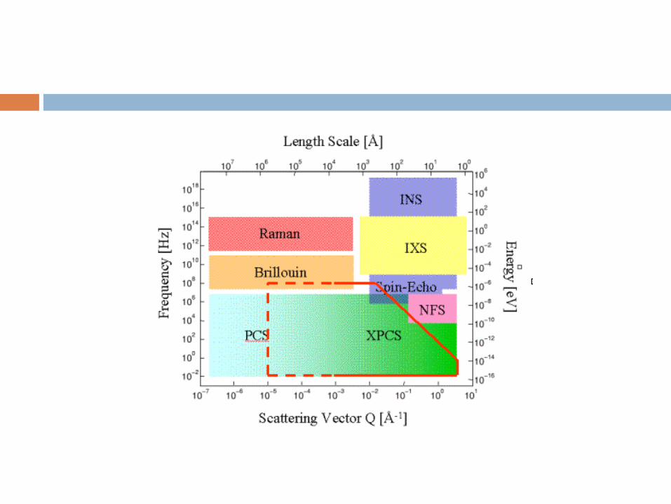
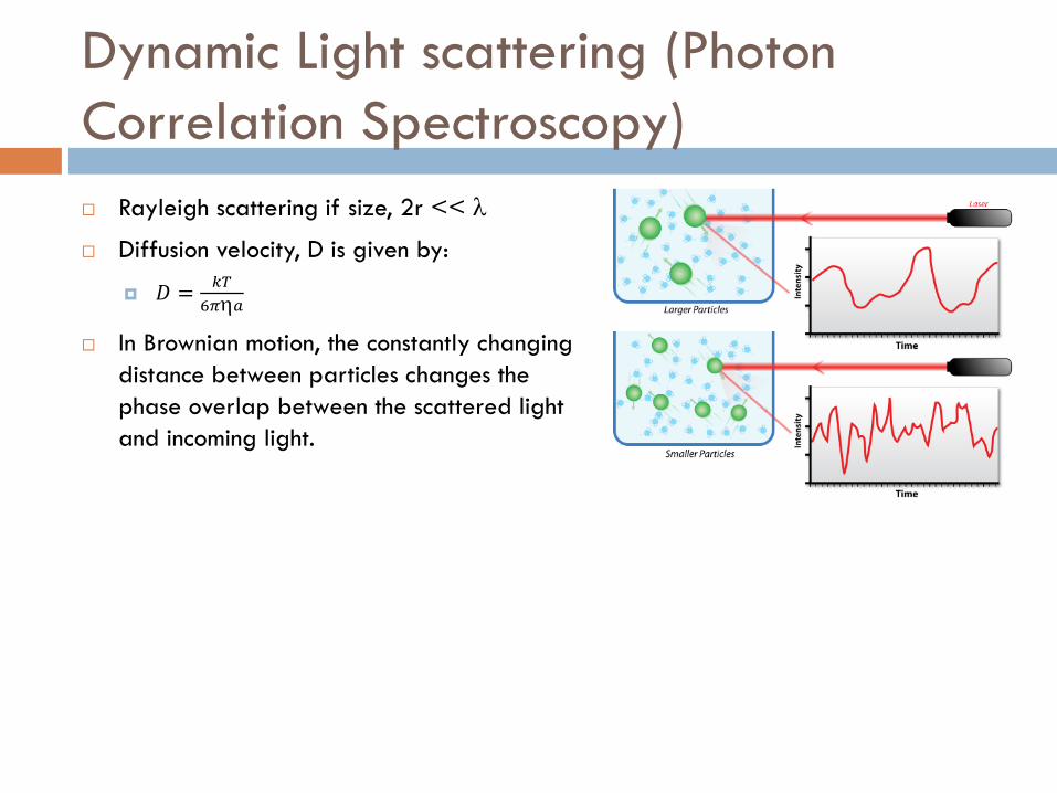
Rayleigh scattering if size, 2r <<

Dynamic Light scattering (Photon
Correlation Spectroscopy)
Rayleigh scattering if size, 2r <<
Diffusion velocity, D is given by:
𝐷 =𝑘𝑇
6𝜋𝑎
Dynamic Light scattering (Photon
Correlation Spectroscopy)
Rayleigh scattering if size, 2r <<
Diffusion velocity, D is given by:
𝐷 =𝑘𝑇
6𝜋𝑎
In Brownian motion, the constantly changing
distance between particles changes the
phase overlap between the scattered light
and incoming light.
Dynamic Light scattering (Photon
Correlation Spectroscopy)
Rayleigh scattering if size, 2r <<
Diffusion velocity, D is given by:
𝐷 =𝑘𝑇
6𝜋𝑎
In Brownian motion, the constantly changing
distance between particles changes the
phase overlap between the scattered light
and incoming light.
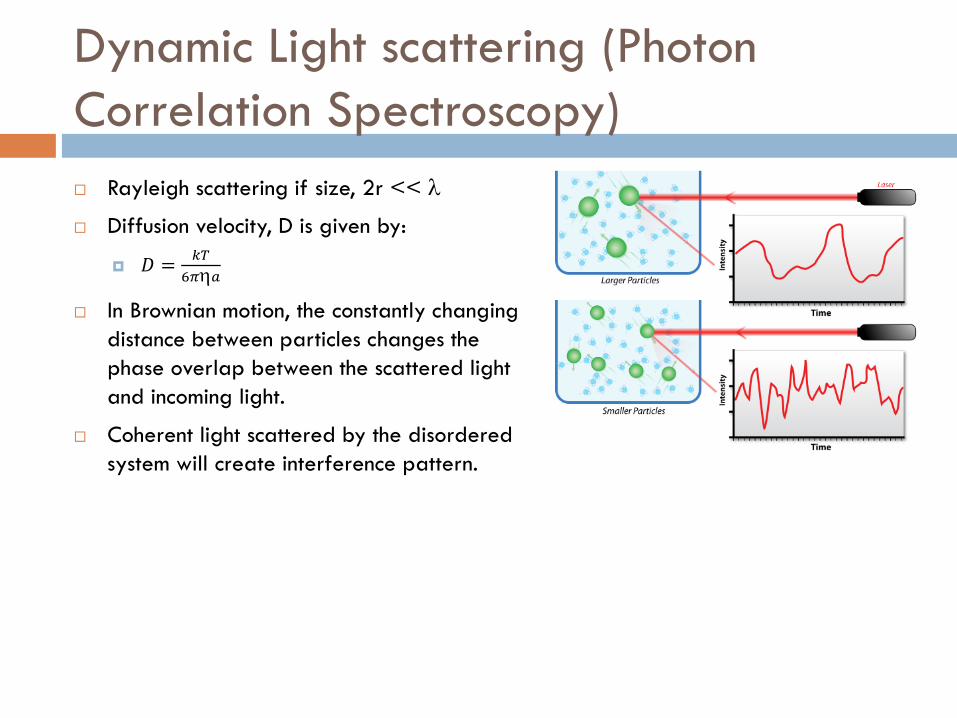
Coherent light scattered by the disordered
system will create interference pattern.

Dynamic Light scattering (Photon
Correlation Spectroscopy)
Rayleigh scattering if size, 2r <<
Diffusion velocity, D is given by:
𝐷 =𝑘𝑇
6𝜋𝑎
In Brownian motion, the constantly changing
distance between particles changes the
phase overlap between the scattered light
and incoming light.
Coherent light scattered by the disordered
system will create interference pattern.
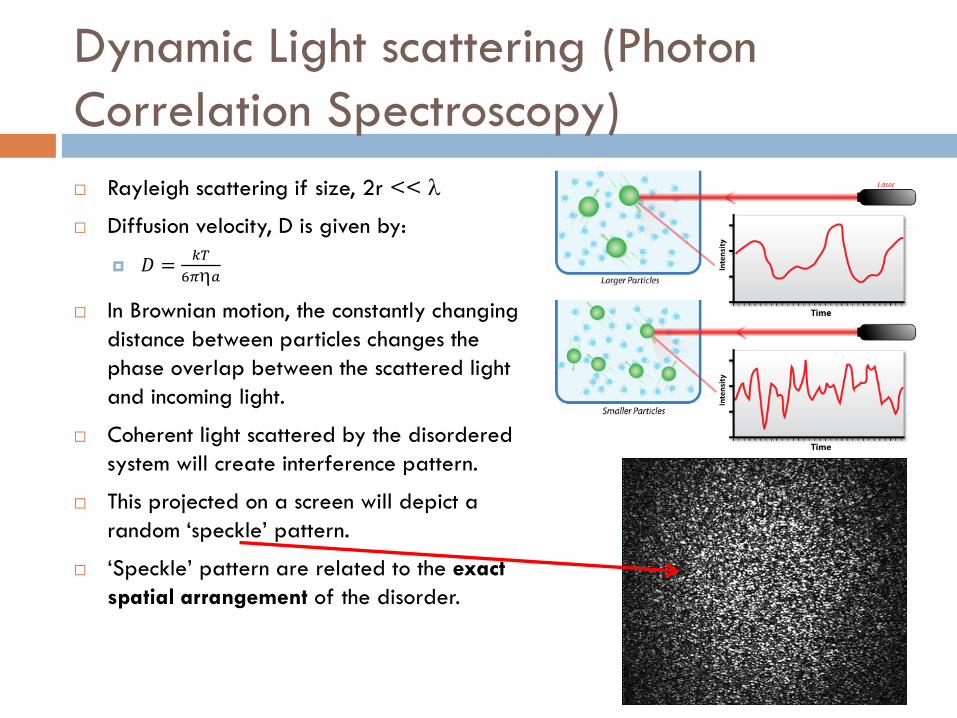
This projected on a screen will depict a
random ‘speckle’ pattern.
Dynamic Light scattering (Photon
Correlation Spectroscopy)
Rayleigh scattering if size, 2r <<
Diffusion velocity, D is given by:
𝐷 =𝑘𝑇
6𝜋𝑎
In Brownian motion, the constantly changing
distance between particles changes the
phase overlap between the scattered light
and incoming light.
Coherent light scattered by the disordered
system will create interference pattern.
This projected on a screen will depict a
random ‘speckle’ pattern.
‘Speckle’ pattern are related to the exact
spatial arrangement of the disorder.
If the spatial arrangement of the disorder changes as a function of time the
“speckle” pattern will also change.
A measurement of the temporal intensity fluctuations of a single or equivalent
speckle is thus a measure of the underlying dynamics.
The temporal intensity fluctuations can be characterized by: Correlation
Spectroscopy Techniques.
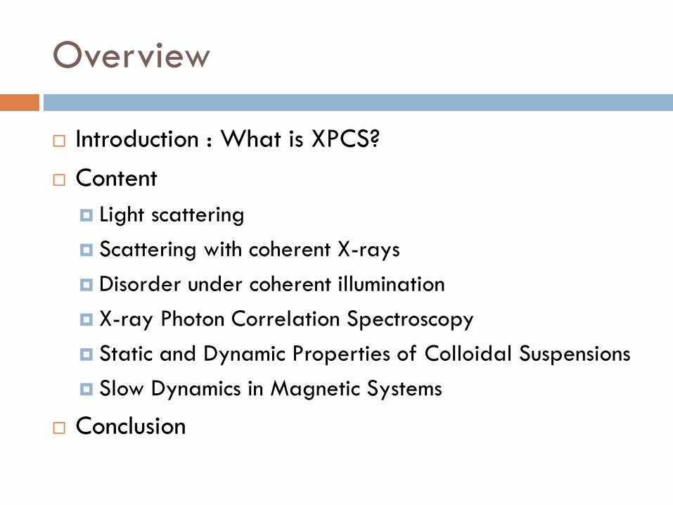
Coherent visible light from a laser source ( ~ 500 nm or 5000 Å ): Photon
Correlation Spectroscopy (PCS) or Dynamic Light Scattering (DLS)
Coherent light from a synchrotron source ( ~ 1Å): X-Ray Photon Correlation
Spectroscopy (XPCS)
Pop-Quiz
What is the order of magnitude of Brilliance in a
3rd generation synchrotron ?
Scattering with coherent X-rays
In a third generation synchrotron, the brilliance, B, is of the order of
1020ph/s/𝑚𝑟𝑎𝑑2/𝑚𝑚2/ 0.1% bandwidth.

Scattering with coherent X-rays
In a third generation synchrotron, the brilliance, B, is of the order of
1020ph/s/𝑚𝑟𝑎𝑑2/𝑚𝑚2/ 0.1% bandwidth.
Using undulators, a fraction of the flux is used as the source for the coherent beam.

Scattering with coherent X-rays
In a third generation synchrotron, the brilliance, B, is of the order of
1020ph/s/𝑚𝑟𝑎𝑑2/𝑚𝑚2/ 0.1% bandwidth.
Using undulators, a fraction of the flux is used as the source for the coherent beam.
The fraction of the ID flux transversely coherent is:
𝐹𝑐 =2
2
𝐵

Scattering with coherent X-rays
In a third generation synchrotron, the brilliance, B, is of the order of
1020ph/s/𝑚𝑟𝑎𝑑2/𝑚𝑚2/ 0.1% bandwidth.
Using undulators, a fraction of the flux is used as the source for the coherent beam.
The fraction of the ID flux transversely coherent is:
𝐹𝑐 =2
2
𝐵
From the textbook (Ch1), we know that:
𝐿𝑇 =2
1
∆where ∆ = 𝑠/𝑅 , is the angular source size
𝐿𝐿 =2
∆
Typically for a third generation sources, 𝐿𝑇 = 10𝜇𝑚 (horizontally) and 100𝜇𝑚(vertically).

Scattering with coherent X-rays
In a third generation synchrotron, the brilliance, B, is of the order of
1020ph/s/𝑚𝑟𝑎𝑑2/𝑚𝑚2/ 0.1% bandwidth.
Using undulators, a fraction of the flux is used as the source for the coherent beam.
The fraction of the ID flux transversely coherent is:
𝐹𝑐 =2
2
𝐵
From the textbook (Ch1), we know that:
𝐿𝑇 =2
1
∆where ∆ = 𝑠/𝑅
𝐿𝐿 =2
∆
Typically for a third generation sources, 𝐿𝑇 = 10𝜇𝑚 (horizontally) and 100𝜇𝑚(vertically).
𝐿𝐿 is also the measure of temporal coherence of the beam and thusly depends on
the monochoromaticity and for perfect crystal ~ 5𝜇𝑚 .
Scattering with coherent X-rays
(cont…)
Requirement of coherent illumination implies that there is a maximum path length
difference (PLD). For XPCS, the two important requirements are:
PLD ≤ 𝐿𝐿
Incident beam size, 𝑑 ≤ 𝐿𝑇
𝑃𝐿𝐷 = 2𝑊 sin2+ 𝑑 sin 2
Scattering with coherent X-rays
(cont…)
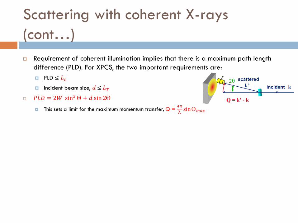
Requirement of coherent illumination implies that there is a maximum path length
difference (PLD). For XPCS, the two important requirements are:
PLD ≤ 𝐿𝐿
Incident beam size, 𝑑 ≤ 𝐿𝑇
𝑃𝐿𝐷 = 2𝑊 sin2+ 𝑑 sin 2
This sets a limit for the maximum momentum transfer, Q = 4𝜋
sin𝑚𝑎𝑥

Scattering with coherent X-rays
(cont…)
Requirement of coherent illumination implies that there is a maximum path length
difference (PLD). For XPCS, the two important requirements are:
PLD ≤ 𝐿𝐿
Incident beam size, 𝑑 ≤ 𝐿𝑇
𝑃𝐿𝐷 = 2𝑊 sin2+ 𝑑 sin 2
This sets a limit for the maximum momentum transfer, Q = 4𝜋
sin𝑚𝑎𝑥

Some details of the setup in ESRF
Slits-Mirror = 44.2 m, Mirror-Piezo mirror = 0.8 m, Piezo-Collimating aperture =
0.5 m, Collimator-sample = 0.1 m, sample-detector = 2m.
The integrated coherent flux through a 12m pinhole is ~ 109 photons/s for =1Å.
The sample distance, 𝑅𝑐 < 𝑑2/ .(?)
Angular size of the individual speckle, 𝐷𝑠 =𝑑
2
+ ∆21/2
Disorder under coherent illumination
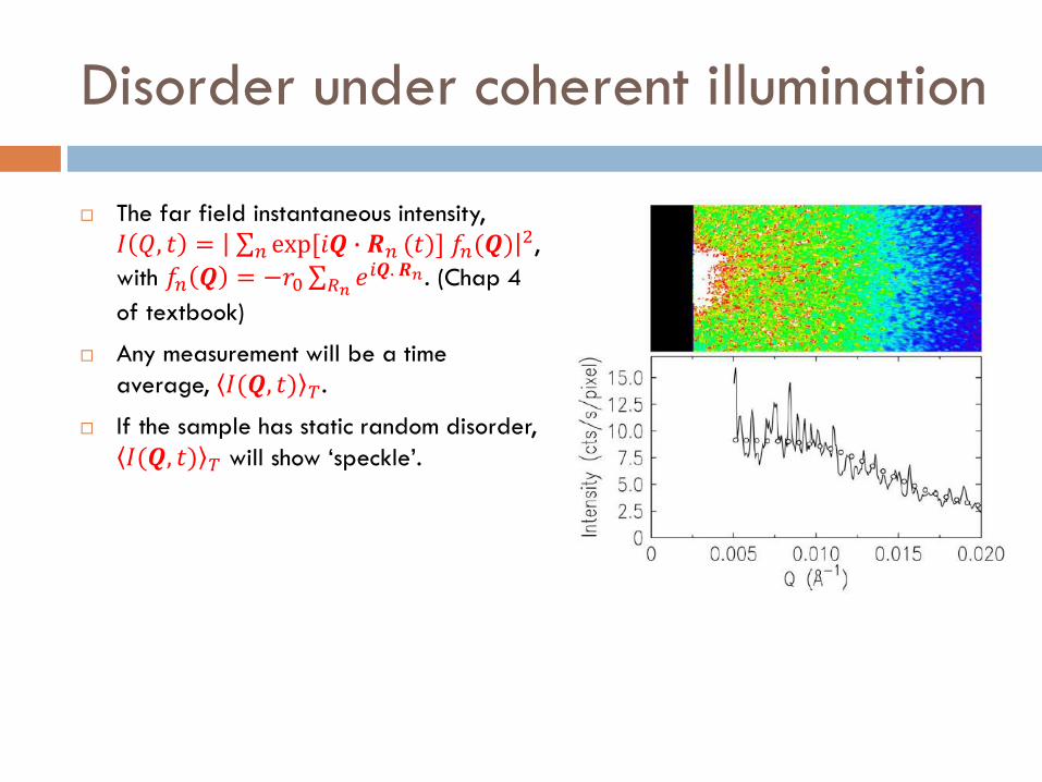
The far field instantaneous intensity,
𝐼 𝑄, 𝑡 = 𝑛 exp[𝑖𝑸 ∙ 𝑹𝑛 (𝑡)] 𝑓𝑛(𝑸)2,
with 𝑓𝑛 𝑸 = −𝑟0 𝑅𝑛 𝑒𝑖𝑸. 𝑹𝑛. (Chap 4
of textbook)
Any measurement will be a time
average, 𝐼(𝑸, 𝑡) 𝑇.
If the sample has static random disorder,
𝐼(𝑸, 𝑡) 𝑇 will show ‘speckle’.

Disorder under coherent illumination
The far field instantaneous intensity,
𝐼 𝑄, 𝑡 = 𝑛 exp[𝑖𝑸 ∙ 𝑹𝑛 (𝑡)] 𝑓𝑛(𝑸)2,
with 𝑓𝑛 𝑸 = −𝑟0 𝑅𝑛 𝑒𝑖𝑸. 𝑹𝑛. (Chap 4
of textbook)
Any measurement will be a time
average, 𝐼(𝑸, 𝑡) 𝑇.
If the sample has static random disorder,
𝐼(𝑸, 𝑡) 𝑇 will show ‘speckle’
Else, 𝐼(𝑸, 𝑡) 𝑇 will just show the envelop
(ensemble average).
X-ray photon correlation Spectroscopy
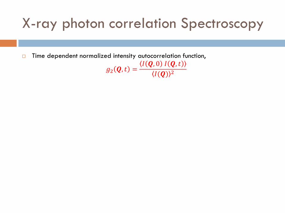
Time dependent normalized intensity autocorrelation function,
𝑔2 𝑸, 𝑡 =𝐼 𝑸, 0 𝐼 𝑸, 𝑡
𝐼(𝑸) 2

X-ray photon correlation Spectroscopy
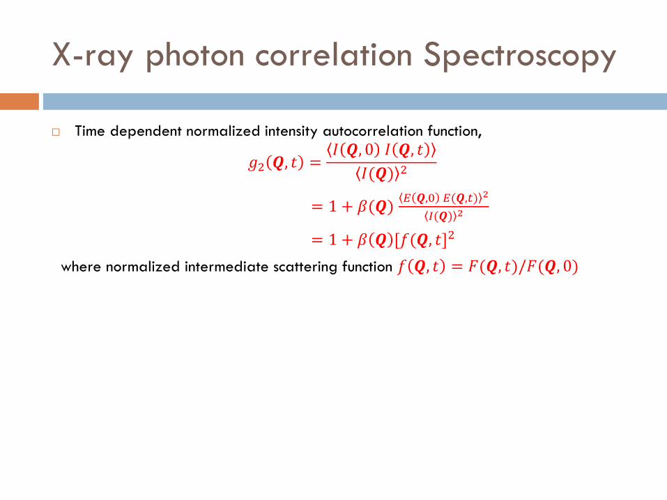
Time dependent normalized intensity autocorrelation function,
𝑔2 𝑸, 𝑡 =𝐼 𝑸, 0 𝐼 𝑸, 𝑡
𝐼(𝑸) 2
= 1 + 𝛽(𝑸)𝐸 𝑸,0 𝐸(𝑸,𝑡) 2
𝐼(𝑸) 2
= 1 + 𝛽 𝑸 [𝑓(𝑸, 𝑡]2
X-ray photon correlation Spectroscopy
Time dependent normalized intensity autocorrelation function,
𝑔2 𝑸, 𝑡 =𝐼 𝑸, 0 𝐼 𝑸, 𝑡
𝐼(𝑸) 2
= 1 + 𝛽(𝑸)𝐸 𝑸,0 𝐸(𝑸,𝑡) 2
𝐼(𝑸) 2
= 1 + 𝛽 𝑸 [𝑓(𝑸, 𝑡]2
where normalized intermediate scattering function 𝑓 𝑸, 𝑡 = 𝐹(𝑸, 𝑡)/𝐹(𝑸, 0)

X-ray photon correlation Spectroscopy
Time dependent normalized intensity autocorrelation function,
𝑔2 𝑸, 𝑡 =𝐼 𝑸, 0 𝐼 𝑸, 𝑡
𝐼(𝑸) 2
= 1 + 𝛽(𝑸)𝐸 𝑸,0 𝐸(𝑸,𝑡) 2
𝐼(𝑸) 2
= 1 + 𝛽 𝑸 [𝑓(𝑸, 𝑡]2
where normalized intermediate scattering function 𝑓 𝑸, 𝑡 = 𝐹(𝑸, 𝑡)/𝐹(𝑸, 0)
Revisiting the example of DLS, 𝑓 𝑸, 𝑡 = exp(−𝐷 𝑄2𝑡)
But, in the presence of particle interaction, 𝑓 𝑸, 𝑡 = exp(−𝐷(𝑄) 𝑄2𝑡)

A plot of ln f(Q,t) vs t.
A useful quantity is the slope of this graph
at t → 0 is . It is define by:
𝑄 = −𝐷 𝑄 𝑄2
Structure and Dynamics of Colloidal
Suspensions
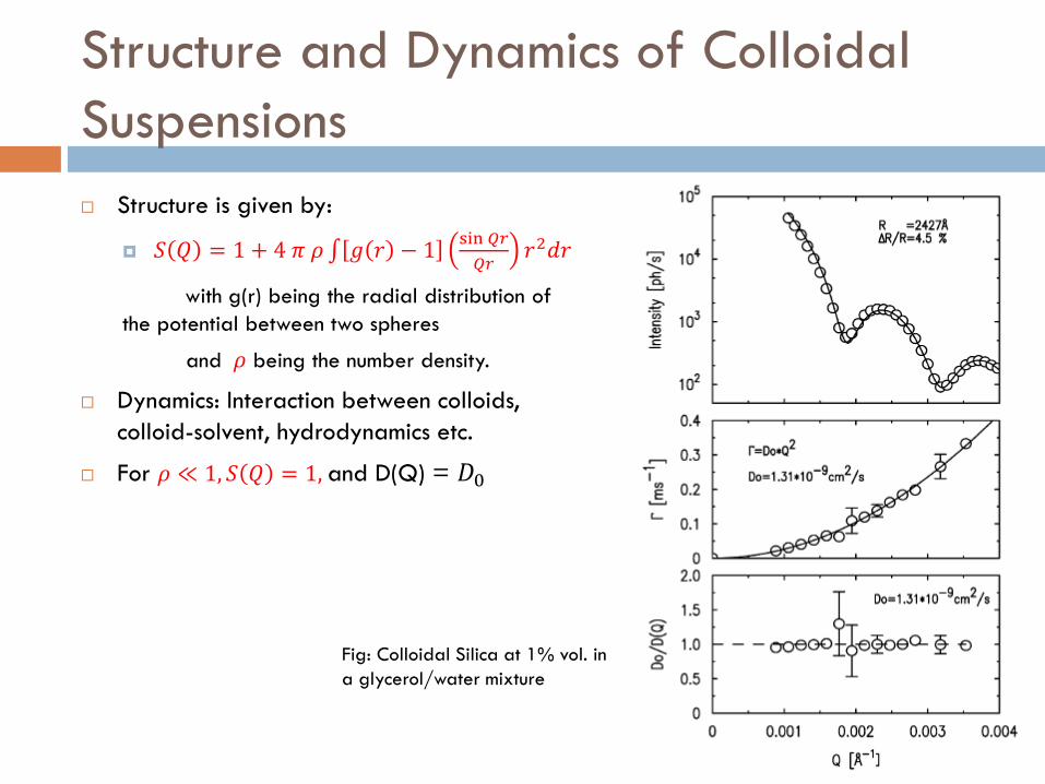
Structure is given by:
𝑆 𝑄 = 1 + 4 𝜋 𝜌 𝑔 𝑟 − 1sin 𝑄𝑟
𝑄𝑟𝑟2𝑑𝑟
with g(r) being the radial distribution of
the potential between two spheres
and 𝜌 being the number density.
Dynamics: Interaction between colloids,
colloid-solvent, hydrodynamics etc.
For 𝜌 ≪ 1, 𝑆 𝑄 = 1, and D(Q) = 𝐷0
Fig: Colloidal Silica at 1% vol. in
a glycerol/water mixture

Structure and Dynamics of Colloidal
Suspensions
Structure is given by:
𝑆 𝑄 = 1 + 4 𝜋 𝜌 𝑔 𝑟 − 1sin 𝑄𝑟
𝑄𝑟𝑟2𝑑𝑟
with g(r) being the radial distribution of
the potential between two spheres
and 𝜌 being the number density.
Dynamics: Interaction between colloids,
colloid-solvent, hydrodynamics etc.
For 𝜌 ≪ 1, 𝑆 𝑄 = 1, and D(Q) = 𝐷0
For higher concentration, D(Q) = 𝐷0 H(Q) /
S(Q)
Fig: Colloidal PMMA at 37%
vol. in cis-decalin mixture

Slow dynamics in Magnetic systems
Magnetic speckles were also
observed in resonant small angle
scattering with soft X-rays.
Soft-xrays were used because of
higher coherence length, thus
higher scattering cross-sections
associated with magnetic
contributions.
Fig: Magnetic speckles observed in resonant
SAXS with soft x-rays from magnetic domain
in 350 Angstrom film of GdFe2 .
Conclusion
Applications:
Condensed matter dynamics
Dynamics of complex fluids
Ultra-slow and non-equilibrium dynamics
2D systems

Conclusion
Applications:
Condensed matter dynamics
Dynamics of complex fluids
Ultra-slow and non-equilibrium dynamics
2D systems
XPCS – Cons:
Need (partially) coherent beam, thus lesser photons than DLS. Low SNRs.
Need fast detectors. Area detectors are too slow, ergo, the title ‘Slow’ dynamics.
X-ray scattering cross-sections are far smaller than laser.
XPCS – Pros:
X-ray wavelengths are much shorter, thus allows larger momentum transfers.
No multiple scattering effects since refractive index is very close to 1.

References
Grubel,G., Zontone, Z., “Correlation spectroscopy with Coherent X-rays”, J. Alloys. Comp. 362
(2004) 3-11.
Sutton, M., Mochrie S., et.el. “Observation of Speckle by Diffraction of X-rays”, Nature 352
(1991) 608.
Grubel,G., Als-Nielsen, J., J. Phys. IV C9(4) (1994) 27.
Als-Nielsen, J., McMorror, D., “Elements of Modern X-ray Physics”, Wiley (2001).
Berne, B., Pecora, R., “Dynamic Light Scattering with Applications”, Wiley (1976).

Questions and Discussion