Fluorescence Correlation Spectroscopy - German … · · 2013-12-03Fluorescence Correlation...
32
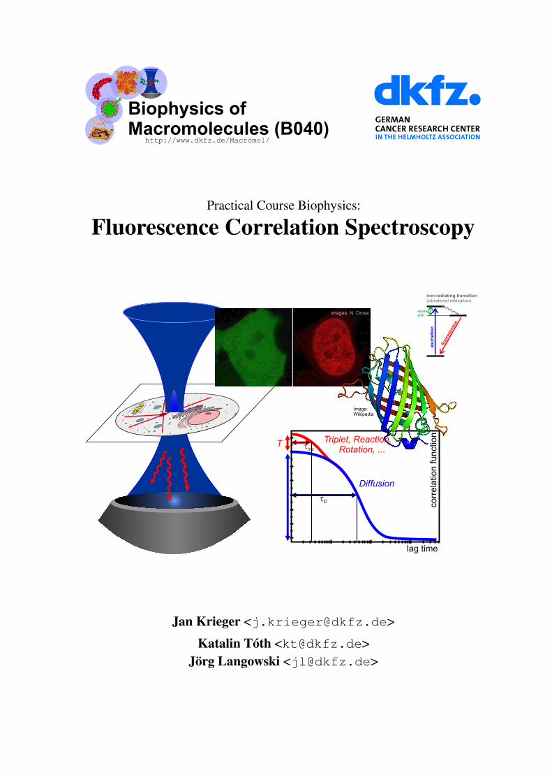
Practical Course Biophysics: Fluorescence Correlation Spectroscopy Jan Krieger <[email protected]> Katalin Tóth <[email protected]> Jörg Langowski <[email protected]>
Transcript of Fluorescence Correlation Spectroscopy - German … · · 2013-12-03Fluorescence Correlation...
Practical Course Biophysics:
Fluorescence Correlation Spectroscopy
Jan Krieger <[email protected]>
Katalin Tóth <[email protected]>Jörg Langowski <[email protected]>
Contents
1 Fluorescence Correlation Spectroscopy (FCS) 31.1 Introduction . . . . . . . . . . . . . . . . . . . . . . . . . . . . . . . . . . . . . 31.2 Theoretical Background . . . . . . . . . . . . . . . . . . . . . . . . . . . . . . . 3
1.2.1 Diffusion . . . . . . . . . . . . . . . . . . . . . . . . . . . . . . . . . . 31.2.2 Particle number fluctuation . . . . . . . . . . . . . . . . . . . . . . . . . 51.2.3 Confocal microscopy . . . . . . . . . . . . . . . . . . . . . . . . . . . . 6
1.3 Autocorrelation analysis . . . . . . . . . . . . . . . . . . . . . . . . . . . . . . 71.3.1 The autocorrelation function of diffusing particles . . . . . . . . . . . . . 81.3.2 The autocorrelation function for multiple diffusing species . . . . . . . . 101.3.3 Effect of triplet dynamics . . . . . . . . . . . . . . . . . . . . . . . . . . . 11
A Preparatory tasks 14
B Tasks during practical course 16
C Useful Data 17C.1 Constants . . . . . . . . . . . . . . . . . . . . . . . . . . . . . . . . . . . . . . 17C.2 Unit conversions . . . . . . . . . . . . . . . . . . . . . . . . . . . . . . . . . . 17C.3 Material properties . . . . . . . . . . . . . . . . . . . . . . . . . . . . . . . . . 18
C.3.1 Water . . . . . . . . . . . . . . . . . . . . . . . . . . . . . . . . . . . . 18C.3.2 Sucrose Solution . . . . . . . . . . . . . . . . . . . . . . . . . . . . . . 19
C.4 Electromagnetic Spectrum . . . . . . . . . . . . . . . . . . . . . . . . . . . . . 20C.5 Fluorophore data . . . . . . . . . . . . . . . . . . . . . . . . . . . . . . . . . . . 21
C.5.1 Alexa-488 . . . . . . . . . . . . . . . . . . . . . . . . . . . . . . . . . . . 21C.5.2 Alexa-594 . . . . . . . . . . . . . . . . . . . . . . . . . . . . . . . . . . 22C.5.3 Enhanced green fluorescing protein (EGFP) . . . . . . . . . . . . . . . . 23C.5.4 Rhodamine 6G . . . . . . . . . . . . . . . . . . . . . . . . . . . . . . . 24
D Mathematical definition of the autocorrelation function 25
E Data Fitting 27
F Anomalous Diffusion 29F.1 Introduction . . . . . . . . . . . . . . . . . . . . . . . . . . . . . . . . . . . . . 29F.2 The autocorrelation function of anomalous diffusion . . . . . . . . . . . . . . . . 30
2
Chapter 1
Fluorescence Correlation Spectroscopy(FCS)
1.1 Introduction
Fluorescence Correlation Spectroscopy (FCS) is a well established technique that allows themeasurement of diffusion coefficients and concentrations for fluorescing constructs. It is alsopossible to retrieve flow speeds and reaction rates. FCS is usually done on a confocal microscopeand may be applied to any fluorescently labeled molecules in solution (usually water or buffersolution), on membranes and even inside living cells.
If the particle of interest is not fluorescing by itself (e.g. autofluorescent proteins), multiplelabeling techniques are available. If proteins are observed one may either create fusion proteinswith autofluorescing molecules (GFP, mRFP, ...) or covalently label the protein with a dye molecule(Alexa dyes, Atto dyes, Rhodamine-6G, Fluoresceine ...) or a quantum dot. If measurements shouldtake place inside living cells fusion proteins come handy, as the cells produce them (stable/transienttransfection) and they are mostly non-toxic. On the other hand autofluorescent proteins are ratherlarge and may therefore influence the dynamic properties and reaction rates of the protein ofinterest. Chemical dyes may easily be attached to DNA and also proteins by linker systems (e.g.biotin/strepdavidin) or reactive side groups of the protein (amine or thiol groups).
The next section will give an introduction into the principle of diffusion (which we observe withFCS in this practical) and the FCS method itself. The most important things that you should knowafter reading these pages are the basic principle of FCS, a feeling for the orders of magnitude of thevariables involved and a rough idea of the setup we are going to use. To check your understandingof FCS, please also go through the questions in section A.
1.2 Theoretical Background
1.2.1 Diffusion
As already mentioned FCS may be used to measure dynamical properties of particles. One of themost important properties is the diffusion coefficient D, as it contains informations about the sizeand weight of the moving particle.
The diffusion coefficient D (units µm2/s) describes how far a particle may reach due to itsdiffusive motion. Diffusion can also be described as a random walk in the solution. While a proteinmoves in water the water molecules collide with the protein and it thus receives a series of smallkicks in random directions. This leads to a random trajectory~r(t) of the individual molecule (for
3
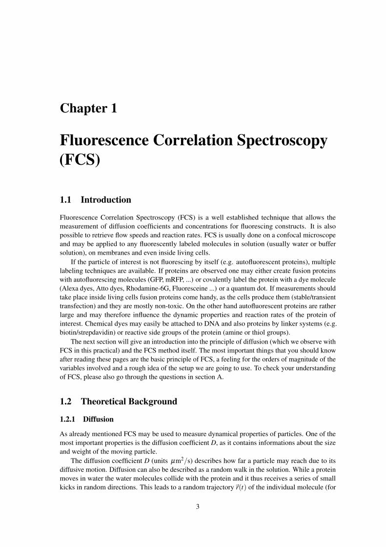
simulation examples, see Fig. 1.1). The larger the diffusion coefficient is, the faster the particlemoves. The trajectory may be characterized by its so called mean squared displacement (MSD)⟨r2⟩, which describes the area that the particle covers in a certain time1. It is linear in time and the
proportionality is given by the diffusion coefficient:⟨r2⟩= 6 ·D · τ. (1.2.1)
We will now show the meaning of this relation: We start with a protein that has a diffusioncoefficient of about D = 50 µm2/s inside the cytoplasm. So to have a good probability of reachingeach position inside the cell (diameter around 20 µm) we will have to let it diffuse for aboutτ ≈ (10 µm)2/(6 ·50 µm2s)≈ 0.3s. This rough estimate already shows that diffusion is sufficientlyfast to serve as a transport process inside cells (e.g. in signal transduction).
Fig. 1.1: Four trajectories of random walks with different diffusion coefficients that increase (red,green, blue, magenta) by a factor of five between two subsequent walks. The circles show the rootmean squared displacement
√〈r2(t)〉 of the particle from its origin, a measure of the area, the
particle covers during the simulation time.
Until the beginning of the 20th century, a macroscopic diffusion law (Fick’s law) was knownthat describes the effects of diffusion (equilibration of concentration gradients), but it could not bederived from microscopic observations (brownian motion). Albert Einstein succeeded in this task.He also derived a relation for the diffusion coefficient, which connects it with the properties of theparticles and the solution they move in. This Stokes-Einstein equation is:
D =kBT
6π ·η ·Rh(1.2.2)
where kB = 1.3806504 · 10−23 J/K is Boltzman’s constant, T is the absolute temperature and η
is the solutions viscosity (see appendix C.1). The particles are describes by their hydrodynamicradius Rh, which is the radius of an equivalent sphere that has the same diffusion coefficient as thegiven molecule. If the molecule is spherical, Rh and the real radius of the molecule will be nearly
1To be more exact, the MSD equals the variance⟨r2⟩ of the trajectory
equal. For molecules with different shape (like e.g. the rod-shaped EGFP), there will be deviations.The hydrodynamic radius will also usually be a bit larger than the real radius of a sphere, as italso takes into account effects like the solvent molecules that are dragged along with the molecule.Note that the temperature dependence of D is not linear, as also the viscosity η shows a strongtemperature dependence. If we assume that the volume Vp of a particle scales linearly with itsmass m, we get that Vp =
43 πR3
h ∝ m. From this we can easily derive the mass-dependence of thediffusion coefficient:
D ∝1
3√
m.
1.2.2 Particle number fluctuation
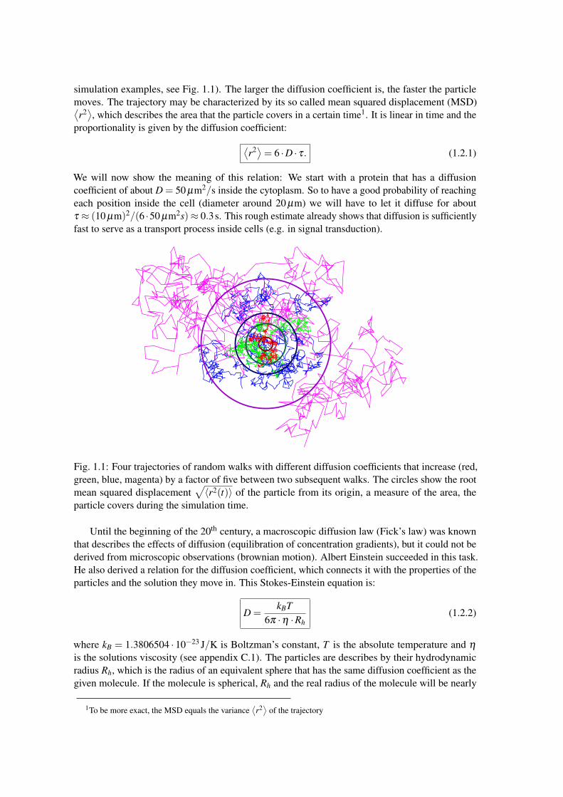
In the last section we have seen that particles move with different speeds. As their movementis not directed, its speed is described by the diffusion coefficient D. We will now discuss howthe diffusion coefficient can be measured experimentally. In this practical course we will use themethod called Fluorescence Correlation Spectroscopy (FCS), which derives the properties of thesample from fluctuations caused by the moving particles. As the name already states, the measuredsignal is the fluorescence intensity I(t) emitted by the observed particles. As we have already seenin section ?? each particle (if excited to the same level) adds the same amount of fluorescence tothe measured signal, so the overall intensity is proportional to the number of particles N we observe.For the further analysis, we will therefore look at the particle number N(t). In FCS we split up theoverall particle number N(t) over time, into an average value 〈N〉 and (small) fluctuations δN(t)around 〈N〉 (see Fig. 1.2, right):
N(t) = 〈N〉+δN(t). (1.2.3)
In FCS, only the fluctuations δN(t) are analyzed, the average 〈N〉 is mostly left out during the dataprocessing. These intensity fluctuations are caused by particles leaving and entering the observationvolume Vobs. If we know how long a particle stays inside the observation volume, we can alsodetermine its diffusion coefficient, which corresponds to its speed. So if we observe particleswith a large D, they will often enter and leave the observation volume in a fixed observation time,and thus show quick fluctuations δN(t). On the other hand these fluctuations will be slower forsmall diffusion coefficients. The correlation analysis performed in FCS extracts the characteristictimescale of these fluctuations which may subsequently be converted into a diffusion coefficient.Figure 1.2 depicts these findings.
Fig. 1.2: Particle number N(t) = 〈N〉+δN(t) in an observation volume for two groups of particles(red, blue) with different diffusion coefficients (Dblue > Dred). Observe the different timescales ofthe fluctuations δN(t).
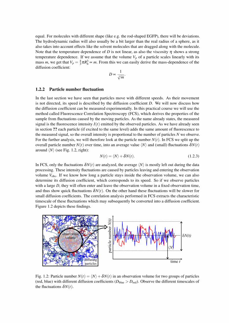
As we want to extract information about the movement of single particles, we have to be ableto detect the fluctuations δNsingle = 1 caused by a single particle entering or leaving the focus. It iseasy to detect this fluctuation caused by one particle if there are only few particles (small N) in theobservation volume. If the average particle number N increases, it becomes more and more difficultto see the fluctuation of one particle and therefore extract valid information about the movementof a single particle. Figure 1.3 shows two examples for this and gives a table with the relativefluctuations δNsingle/N = 1/N for different average particle numbers in the detection volume. ForN = 100 the relative fluctuation have already dropped to only 1%. For particle numbers above thisvalue they are hardly detectable.
Fig. 1.3: Relative particle number fluctuations δNsingle/N of one particle entering or leaving avolume with N particles on average.
Using these results we can estimate the typical volume Vsample and concentration csample of thesample, that we will have to use. In a typical fluorimeter the volume of the cuvette is Vsample =100 µl and the typical sample concentration is csample = 100nM (i.e. 〈N〉 = 100 · 10−9 · 6.022 ·1023 ·100 ·10−6 ≈ 6 ·1012 particles in the cuvette). Here the relative fluctuations are only about4 · 10−7 = 0.00004% which is way too low to give valid results. To come past these problemswe could either reduce the sample concentration, or the observation volume. If we stick to ourcuvette, we would have to go concentrations of 10−22 M which is impracticably low (for this valuewe would be left with about 20 molecules in the cuvette). So we will have to reduce the samplevolume. If we could go as low as Vsample1fl = 10−15 l = 1 µm3 we get around 10 particles in thisvolume for a reasonable concentration of csample18nM.
So far we have seen that we can extract information about the motion of particles in solution, ifwe observe their particle number fluctuations, while particles move in and out of a small volume.As the relative fluctuations get smaller with increasing particle number we have to use small particlenumbers. We have estimated that the volume has to be around Vsample1fl if we still want to workat reasonable concentration in the nano-molar range. Such volumes may be realized, if we use aconfocal microscope, which is a common instrument for biological imaging. The next section willbriefly explain the setup of such an instrument.
1.2.3 Confocal microscopy
In FCS the prerequisite of small system volumes is usually achieved by using a confocal microscopewith an objective of high numerical aperture (NA > 0.9). The focal volume obtained by this setup ison the order of 1fl = 10−15 l = 1 µm3. Figure 1.4 shows the optical setup of a confocal microscope.Incident excitation light (blue) is focused by an objective lens into the sample. The size d of thefocus may be approximated by Abbe’s law, which states that
d =λ
2 ·n ·NA(1.2.4)
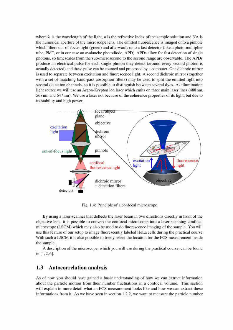
where λ is the wavelength of the light, n is the refractive index of the sample solution and NA isthe numerical aperture of the microscope lens. The emitted fluorescence is imaged onto a pinholewhich filters out-of-focus light (green) and afterwards onto a fast detector (like a photo-multipliertube, PMT, or in our case an avalanche photodiode, APD). APDs allow for fast detection of singlephotons, so timescales from the sub-microsecond to the second range are observable. The APDsproduce an electrical pulse for each single photon they detect (around every second photon isactually detected) and these pulse can be counted and processed by a computer. One dichroic mirroris used to separate between excitation and fluorescence light. A second dichroic mirror (togetherwith a set of matching band-pass absorption filters) may be used to split the emitted light intoseveral detection channels, so it is possible to distinguish between several dyes. As illuminationlight source we will use an Argon-Krypton ion laser which emits on three main laser lines (488nm,568nm and 647nm). We use a laser not because of the coherence properties of its light, but due toits stability and high power.
Fig. 1.4: Principle of a confocal microscope
By using a laser-scanner that deflects the laser beam in two directions directly in front of theobjective lens, it is possible to convert the confocal microscope into a laser-scanning confocalmicroscope (LSCM) which may also be used to do fluorescence imaging of the sample. You willuse this feature of our setup to image fluorescently labeled HeLa cells during the practical course.With such a LSCM it is also possible to freely select the location for the FCS measurement insidethe sample.
A description of the microscope, which you will use during the practical course, can be foundin [1, 2, 6].
1.3 Autocorrelation analysis
As of now you should have gained a basic understanding of how we can extract informationabout the particle motion from their number fluctuations in a confocal volume. This sectionwill explain in more detail what an FCS measurement looks like and how we can extract theseinformations from it. As we have seen in section 1.2.2, we want to measure the particle number
fluctuations N(t) = 〈N〉+ δN(t) of fluorescing molecules entering and leaving the focus of aconfocal microscope. As we cannot directly count the number of particles, we measure thefluorescence intensity I(t) emitted by the particles currently inside the focus and analyse this.While a particle is inside the focus, it is excited by the laser of the microscope and thereforeconstantly cycles between its ground and excited state (it stays around 1...10ns in the excited state,the fluorescence lifetime, see section ??). In each cycle a fluorescence photon is emitted in arandom spacial direction. A fraction of these photons is then collected by the objective lens andsubsequently detected on an APD. The output of the APD, we will call I(t). Therefore the intensityI(t) fluctuates in the same way, as the particle number N(t) and every property we derived for N(t)is also valid for I(t). We can also split it into a constant offset 〈I〉 and the fluctuations δ I(t) (seee.g. Fig. 1.5, left panels) :
I(t) = 〈I〉+δ I(t)
From this measured signal, we now have to extract how fast it fluctuates, in order to gain informationon how fast the particles move in the sample (see section 1.2.2 and especially 1.2). To do this,we use a mathematical tool, called autocorrelation analysis (therefore also the name fluorescencecorrelation spectroscopy, FCS). In FCS a special computer card calculates the autocorrelationfunction g(τ) from the intensity signal I(t) measured in the microscope. The autocorrelationfunction is mathematically defined as:
g(τ) =〈δ I(t) ·δ I(t + τ)〉t
〈I(t)〉2t, (1.3.1)
where 〈...〉t denotes a time average over the time variable t:
〈I(t)〉t =1T
T∫1
I(t)dt
It measures the self-similarity of the fluctuations δ I(t), if compared to itself, a time τ (lag time)later. If we look at the fluctuations δ I(t) and δ I(t + τ) with a long lag time τ , we do not detect anyself-similarity in the signal, as the fluctuations at time t + τ are caused by different particles than attime t, which are independent of each other. So the autocorrelation g(tτ) should be small (around0). In contrast, if the lag time τ is so small, that the same particles create the fluctuations at timet and t + τ (so smaller than the average retention time of the particles in the focus), we will havesome degree of self-similarity between δ I(t) and δ I(t + τ) (high autocorrelation g(τ > 0).
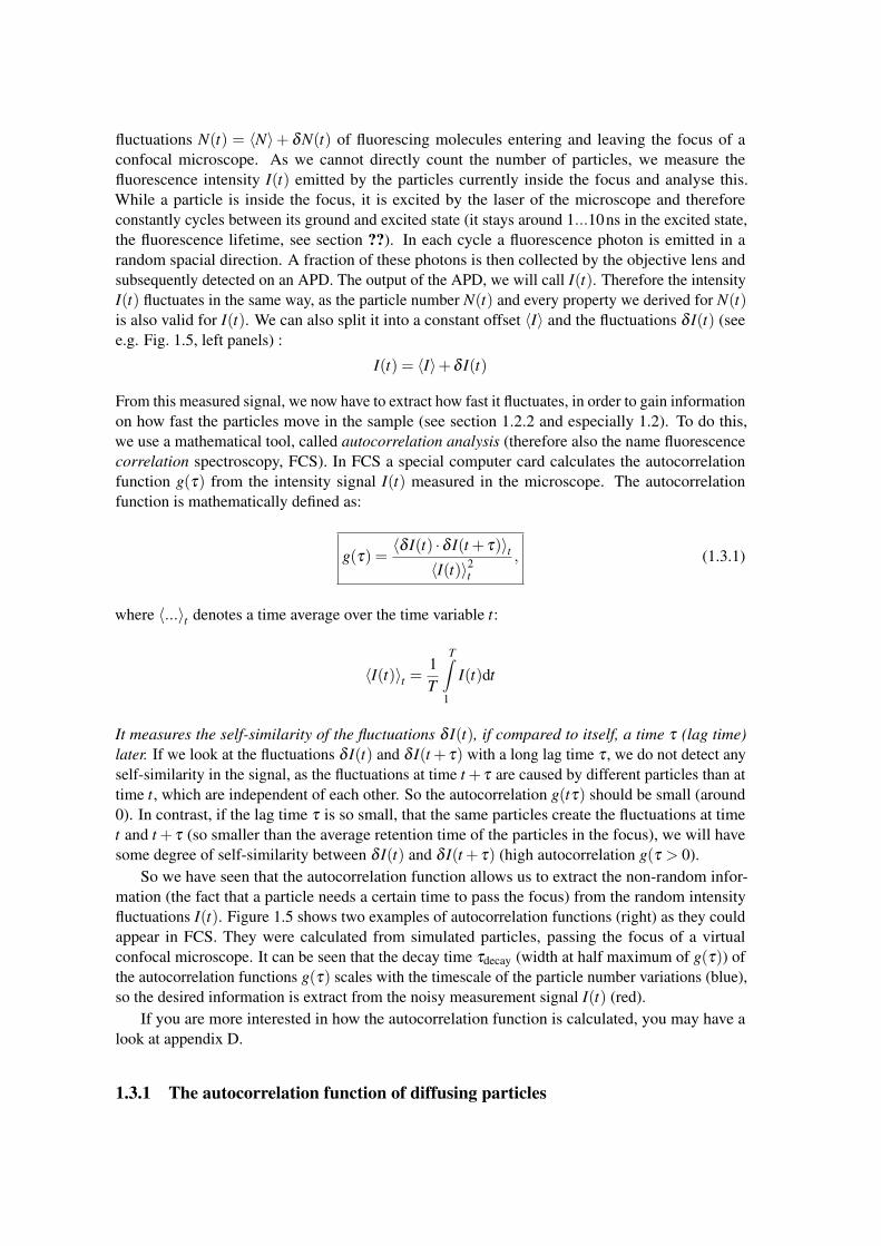
So we have seen that the autocorrelation function allows us to extract the non-random infor-mation (the fact that a particle needs a certain time to pass the focus) from the random intensityfluctuations I(t). Figure 1.5 shows two examples of autocorrelation functions (right) as they couldappear in FCS. They were calculated from simulated particles, passing the focus of a virtualconfocal microscope. It can be seen that the decay time τdecay (width at half maximum of g(τ)) ofthe autocorrelation functions g(τ) scales with the timescale of the particle number variations (blue),so the desired information is extract from the noisy measurement signal I(t) (red).
If you are more interested in how the autocorrelation function is calculated, you may have alook at appendix D.
1.3.1 The autocorrelation function of diffusing particles
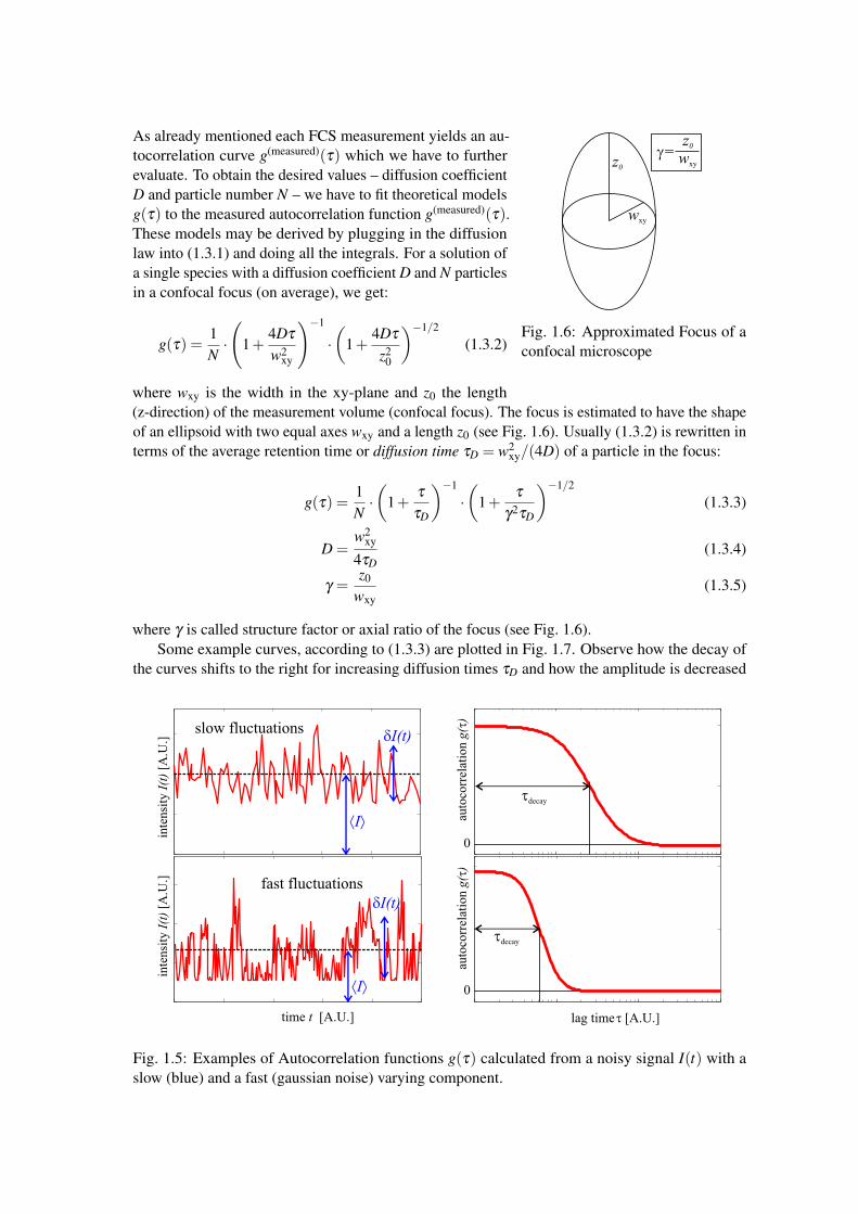
Fig. 1.6: Approximated Focus of aconfocal microscope
As already mentioned each FCS measurement yields an au-tocorrelation curve g(measured)(τ) which we have to furtherevaluate. To obtain the desired values – diffusion coefficientD and particle number N – we have to fit theoretical modelsg(τ) to the measured autocorrelation function g(measured)(τ).These models may be derived by plugging in the diffusionlaw into (1.3.1) and doing all the integrals. For a solution ofa single species with a diffusion coefficient D and N particlesin a confocal focus (on average), we get:
g(τ) =1N·
(1+
4Dτ
w2xy
)−1
·(
1+4Dτ
z20
)−1/2
(1.3.2)
where wxy is the width in the xy-plane and z0 the length(z-direction) of the measurement volume (confocal focus). The focus is estimated to have the shapeof an ellipsoid with two equal axes wxy and a length z0 (see Fig. 1.6). Usually (1.3.2) is rewritten interms of the average retention time or diffusion time τD = w2
xy/(4D) of a particle in the focus:
g(τ) =1N·(
1+τ
τD
)−1
·(
1+τ
γ2τD
)−1/2
(1.3.3)
D =w2
xy
4τD(1.3.4)
γ =z0
wxy(1.3.5)
where γ is called structure factor or axial ratio of the focus (see Fig. 1.6).Some example curves, according to (1.3.3) are plotted in Fig. 1.7. Observe how the decay of
the curves shifts to the right for increasing diffusion times τD and how the amplitude is decreased
Fig. 1.5: Examples of Autocorrelation functions g(τ) calculated from a noisy signal I(t) with aslow (blue) and a fast (gaussian noise) varying component.
for increasing particle numbers N. In fact the amplitude approaches the value g(0) = 1/N, so onecan read the inverse particle number directly from the extrapolated zero-lag correlation. This againshows that the correlation gets less and less pronounced (low amplitude) for large particle numbersN. Also the diffusion time can directly be estimated from the graphs, by reading the width of thecorrelation function at half its amplitude g(0).
Fig. 1.7: Autocorrelation function for simple diffusion. Left: N = 10 particles and increasingdiffusion time, Right: increasing particle number with diffusion times τD = 100 µs
In order to calculate the diffusion coefficient D we have to know the lateral size of the focuswxy and the structure factor γ . The latter one has been determined for our instrument from an imagestack of immobile particles to be γ ≈ 6. This value is not prone to large deviations due to slightmisalignment, so you can simply use the given value for the data evaluation. The size of the focuswxy is determined by a calibration measurement of a solution with known diffusion coefficient (inour lab usually Alexa-488), which has to be redone on a day-to-day basis, or when parts of thesetup change (sample chamber...). Knowing the size of the focus, we can also estimate its volumeVeff and therefore the concentration c of the solution:
Veff = π3/2 ·w2
xy · z0 = π3/2 · γ ·w3
xy (1.3.6)
c =N
Veff(1.3.7)
1.3.2 The autocorrelation function for multiple diffusing species
The autocorrelation function (1.3.3) can be extended to a case where k species with differentdiffusion times τD,i are present:
g(τ) =1N·
k
∑i=1
ρi ·(
1+τ
τD,i
)−1
·(
1+τ
γ2τD,i
)−1/2
(1.3.8)
k
∑i=1
ρi = 1, and 0≤ ρi ≤ 1
N is the overall particle number in the focus and the ρi characterize the fraction of particles ofspecies i. If all species have fluorophores of the same quantum yield φi ≡ φ (see section ??), ρi in(1.3.8) directly equals the fraction of particles of the i-th species. So Ni = ρi ·N particles of species
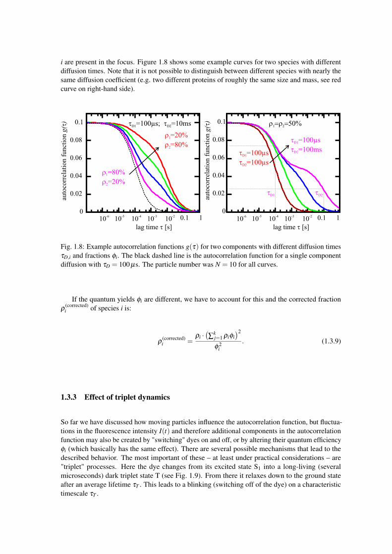
i are present in the focus. Figure 1.8 shows some example curves for two species with differentdiffusion times. Note that it is not possible to distinguish between different species with nearly thesame diffusion coefficient (e.g. two different proteins of roughly the same size and mass, see redcurve on right-hand side).
Fig. 1.8: Example autocorrelation functions g(τ) for two components with different diffusion timesτD,i and fractions φi. The black dashed line is the autocorrelation function for a single componentdiffusion with τD = 100 µs. The particle number was N = 10 for all curves.
If the quantum yields φi are different, we have to account for this and the corrected fractionρ
(corrected)i of species i is:
ρ(corrected)i =
ρi ·(∑
kj=1 ρiφi
)2
φ 2i
. (1.3.9)
1.3.3 Effect of triplet dynamics
So far we have discussed how moving particles influence the autocorrelation function, but fluctua-tions in the fluorescence intensity I(t) and therefore additional components in the autocorrelationfunction may also be created by "switching" dyes on and off, or by altering their quantum efficiencyφi (which basically has the same effect). There are several possible mechanisms that lead to thedescribed behavior. The most important of these – at least under practical considerations – are"triplet" processes. Here the dye changes from its excited state S1 into a long-living (severalmicroseconds) dark triplet state T (see Fig. 1.9). From there it relaxes down to the ground stateafter an average lifetime τT . This leads to a blinking (switching off of the dye) on a characteristictimescale τT .
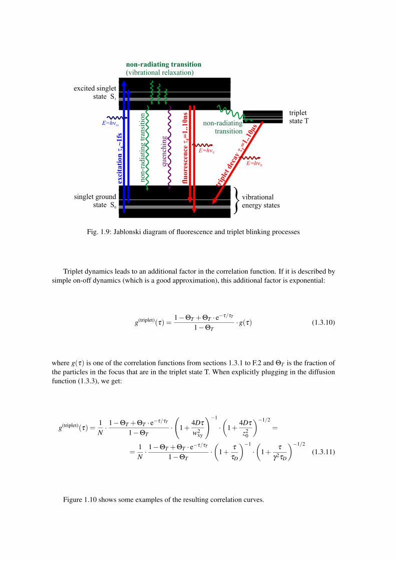
Fig. 1.9: Jablonski diagram of fluorescence and triplet blinking processes
Triplet dynamics leads to an additional factor in the correlation function. If it is described bysimple on-off dynamics (which is a good approximation), this additional factor is exponential:
g(triplet)(τ) =1−ΘT +ΘT · e−τ/τT
1−ΘT·g(τ) (1.3.10)
where g(τ) is one of the correlation functions from sections 1.3.1 to F.2 and ΘT is the fraction ofthe particles in the focus that are in the triplet state T. When explicitly plugging in the diffusionfunction (1.3.3), we get:
g(triplet)(τ) =1N· 1−ΘT +ΘT · e−τ/τT
1−ΘT·
(1+
4Dτ
w2xy
)−1
·(
1+4Dτ
z20
)−1/2
=
=1N· 1−ΘT +ΘT · e−τ/τT
1−ΘT·(
1+τ
τD
)−1
·(
1+τ
γ2τD
)−1/2
(1.3.11)
Figure 1.10 shows some examples of the resulting correlation curves.
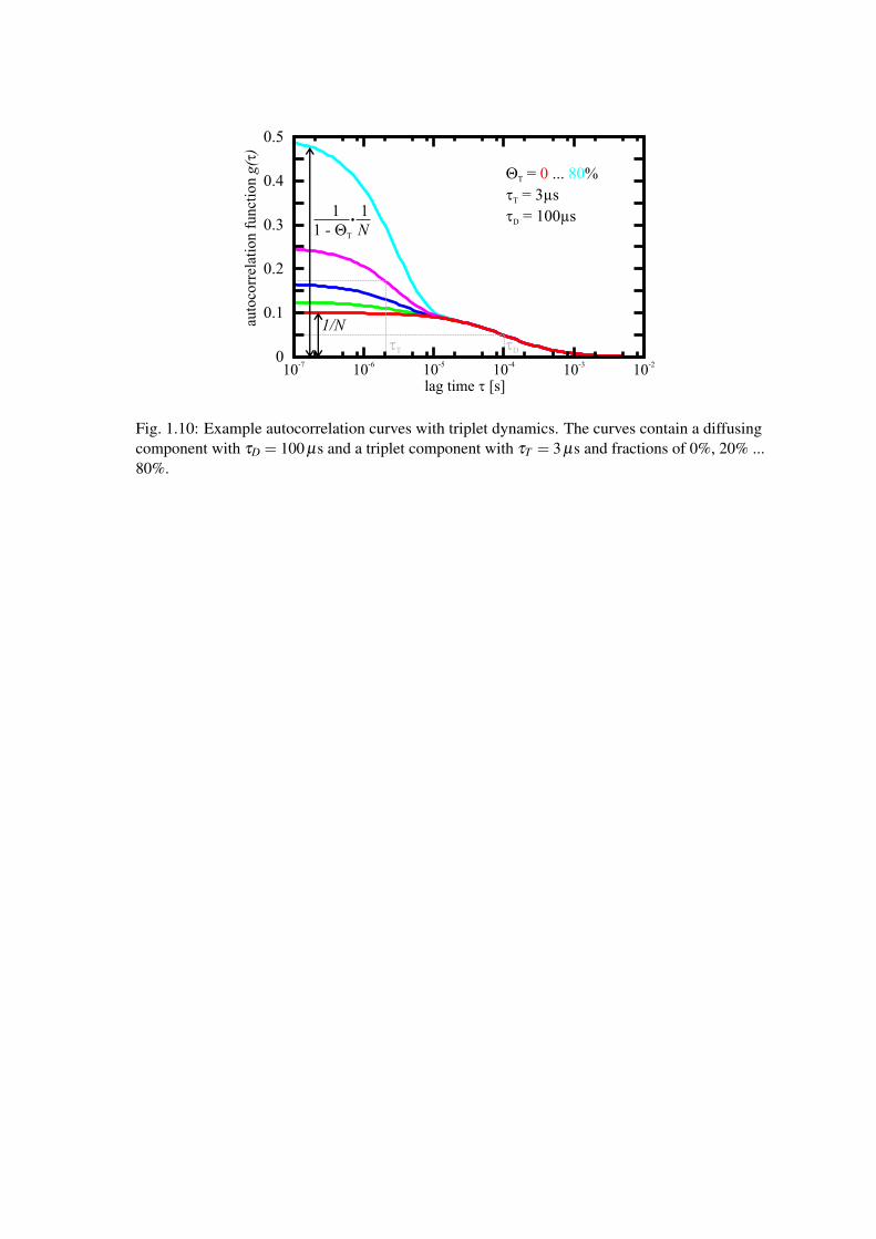
Fig. 1.10: Example autocorrelation curves with triplet dynamics. The curves contain a diffusingcomponent with τD = 100 µs and a triplet component with τT = 3 µs and fractions of 0%, 20% ...80%.
Appendix A
Preparatory tasks
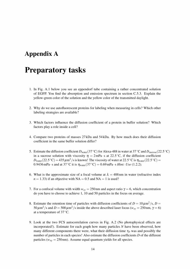
1. In Fig. A.1 below you see an eppendorf tube containing a rather concentrated solutionof EGFP. You find the absorption and emission spectrum in section C.5.3. Explain theyellow-green color of the solution and the yellow color of the transmitted daylight.
2. Why do we use autofluorescent proteins for labeling when measuring in cells? Which otherlabeling strategies are available?
3. Which factors influence the diffusion coefficient of a protein in buffer solution? Whichfactors play a role inside a cell?
4. Compare two proteins of masses 27kDa and 54kDa. By how much does their diffusioncoefficient in the same buffer solution differ?
5. Estimate the diffusion coefficient Dwater(37 ◦C) for Alexa-488 in water at 37 ◦C and Dsucrose(22.5 ◦C)in a sucrose solution with viscosity η = 2mPa · s at 22.5 ◦C, if the diffusion coefficientDwater(22.5 ◦C)= 435 µm2/s is known! The viscosity of water at 22.5 ◦C is ηwater(22.5 ◦C)=0.9436mPa · s and at 37 ◦C it is ηwater(37 ◦C) = 0.69mPa · s Hint: Use (1.2.2).
6. What is the approximate size of a focal volume at λ = 488nm in water (refractive indexn = 1.33) if an objective with NA = 0.5 and NA = 1 is used?
7. For a confocal volume with width wxy = 250nm and aspect ratio γ = 6, which concentrationdo you have to choose to achieve 1, 10 and 50 particles in the focus on average.
8. Estimate the retention time of particles with diffusion coefficients of D = 10 µm2/s, D =50 µm2/s and D = 500 µm2/s inside the above described laser focus (wxy = 250nm, γ = 6)at a temperature of 37 ◦C.
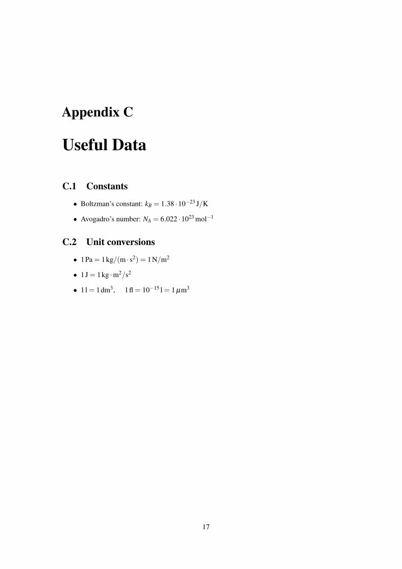
9. Look at the two FCS autocorrelation curves in Fig. A.2 (No photophysical effects areincorporated!). Estimate for each graph how many particles N have been observed, howmany different components there were, what their diffusion time τD was and possibly thenumber of particles in each species! Also estimate the diffusion coefficients D of the differentparticles (wxy = 250nm). Assume equal quantum yields for all species.
14
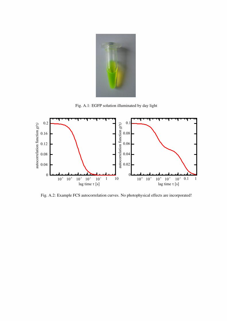
Fig. A.1: EGFP solution illuminated by day light
Fig. A.2: Example FCS autocorrelation curves. No photophysical effects are incorporated!

Appendix B
Tasks during practical course
• fluorescence correlation spectroscopy (FCS):
– Calibration measurement with 20nM Alexa-488 solution (every day and for every typeof sample chamber!)
– Dilution series with Alexa-488, using 500nM, 200nM, 50nM, 20nM, 2nM, 0.2nMsolutions. Determine the dependence of N and the diffusion coefficient D on thesample concentration. What do you observe? What is a good sample concentration toperform FCS? Does the amount of light in the lab change the results? Measure also thebackground inetnsity (measured intensity without sample).
– Determination of diffusion coefficient D and hydrodynamic radius Rh of differentsamples in solution (e.g.: EGFP-monomers, EGFP-tetramers, quantum dots, latexbeads, labeled DNA, ...). Also look at the molecular brightnes (average countratedivided by the number of particles) for different dyes and for the same dye free insolution and bound to a target molecule (e.g. Alexa-488, bound to DNA).
– Measure the diffusion of Alexa-488 in 20% sucrose solution. What changes? How canyou correct for artifacts? See also appendix C.3.2.
– Measurement of a mixture of two fluorescing molecules with different molecularweights. Can you recover the expected diffusion coefficients and particle numberfractions ρi?
– FCS measurement of EGFP mono- and tetramers (1xEGFP, 4xEGFP) in HeLa cells.Which fit model describes your data best? Which would you choose? How do theresults differ for different positions in the cells and mono- and tetramers? Compareyour results to the measurements of 1xEGFP/4xEGPF in solution!
16
Appendix C
Useful Data
C.1 Constants
• Boltzman’s constant: kB = 1.38 ·10−23 J/K
• Avogadro’s number: NA = 6.022 ·1023 mol−1
C.2 Unit conversions
• 1Pa = 1kg/(m · s2) = 1N/m2
• 1J = 1kg ·m2/s2
• 1l = 1dm3, 1fl = 10−15 l = 1 µm3
17
C.3 Material properties
C.3.1 Water
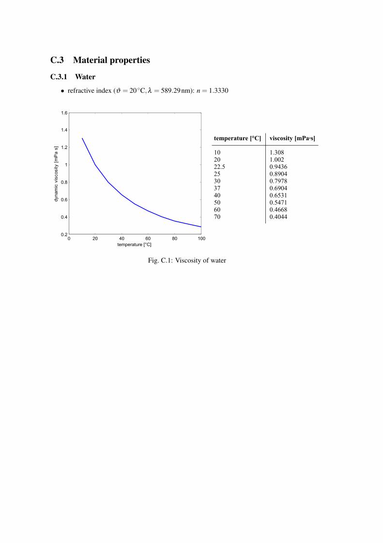
• refractive index (ϑ = 20 ◦C,λ = 589.29nm): n = 1.3330
Fig. C.1: Viscosity of water
C.3.2 Sucrose Solution
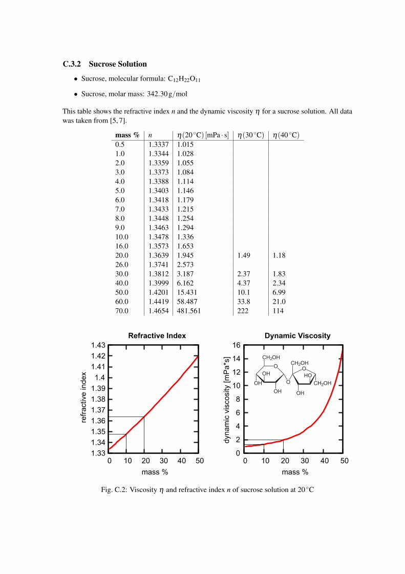
• Sucrose, molecular formula: C12H22O11
• Sucrose, molar mass: 342.30g/mol
This table shows the refractive index n and the dynamic viscosity η for a sucrose solution. All datawas taken from [5, 7].
mass % n η(20 ◦C) [mPa · s] η(30 ◦C) η(40 ◦C)0.5 1.3337 1.0151.0 1.3344 1.0282.0 1.3359 1.0553.0 1.3373 1.0844.0 1.3388 1.1145.0 1.3403 1.1466.0 1.3418 1.1797.0 1.3433 1.2158.0 1.3448 1.2549.0 1.3463 1.29410.0 1.3478 1.33616.0 1.3573 1.65320.0 1.3639 1.945 1.49 1.1826.0 1.3741 2.57330.0 1.3812 3.187 2.37 1.8340.0 1.3999 6.162 4.37 2.3450.0 1.4201 15.431 10.1 6.9960.0 1.4419 58.487 33.8 21.070.0 1.4654 481.561 222 114
Fig. C.2: Viscosity η and refractive index n of sucrose solution at 20 ◦C
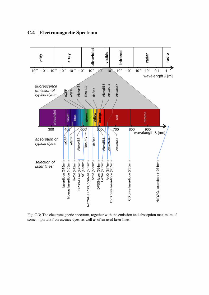
C.4 Electromagnetic Spectrum
Fig. C.3: The electromagnetic spectrum, together with the emission and absorption maximum ofsome important fluorescence dyes, as well as often used laser lines.
C.5 Fluorophore data
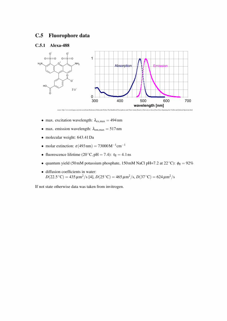
C.5.1 Alexa-488
• max. excitation wavelength: λex,max = 494nm
• max. emission wavelength: λem,max = 517nm
• molecular weight: 643.41Da
• molar extinction: ε(493nm) = 73000M−1cm−1
• fluorescence lifetime (20 ◦C,pH = 7.4): τfl = 4.1ns
• quantum yield (50mM potassium phosphate, 150mM NaCl pH=7.2 at 22 ◦C): φfl = 92%
• diffusion coefficients in water:D(22.5 ◦C) = 435 µm2/s [4], D(25 ◦C) = 465 µm2/s, D(37 ◦C) = 624 µm2/s
If not state otherwise data was taken from invitrogen.
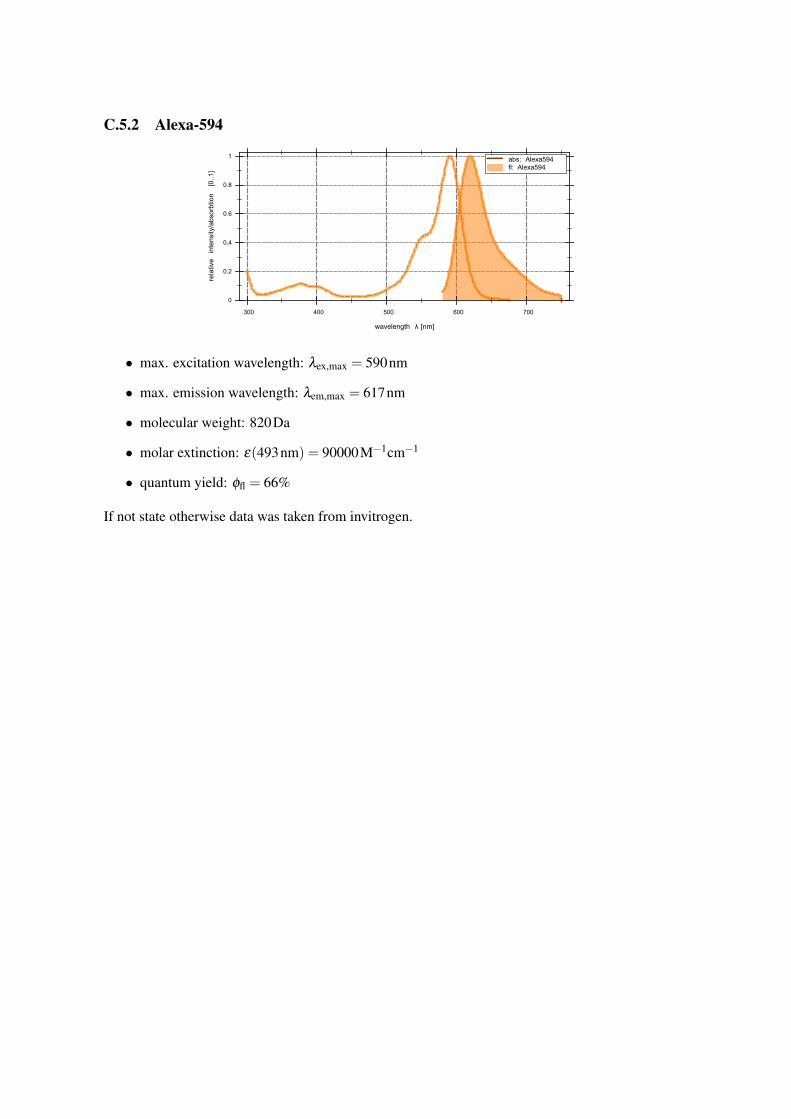
C.5.2 Alexa-594
300 400 500 600 700
wavelength λ [nm]
0
0.2
0.4
0.6
0.8
1
rela
tive
inte
nsi
ty/a
bso
rbtio
n
[0..1]
abs: Alexa594fl: Alexa594
• max. excitation wavelength: λex,max = 590nm
• max. emission wavelength: λem,max = 617nm
• molecular weight: 820Da
• molar extinction: ε(493nm) = 90000M−1cm−1
• quantum yield: φfl = 66%
If not state otherwise data was taken from invitrogen.
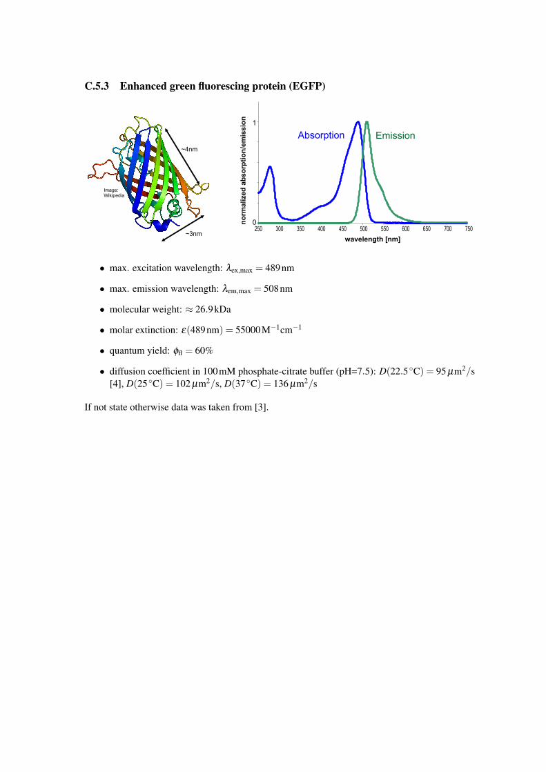
C.5.3 Enhanced green fluorescing protein (EGFP)
• max. excitation wavelength: λex,max = 489nm
• max. emission wavelength: λem,max = 508nm
• molecular weight: ≈ 26.9kDa
• molar extinction: ε(489nm) = 55000M−1cm−1
• quantum yield: φfl = 60%
• diffusion coefficient in 100mM phosphate-citrate buffer (pH=7.5): D(22.5 ◦C) = 95 µm2/s[4], D(25 ◦C) = 102 µm2/s, D(37 ◦C) = 136 µm2/s
If not state otherwise data was taken from [3].
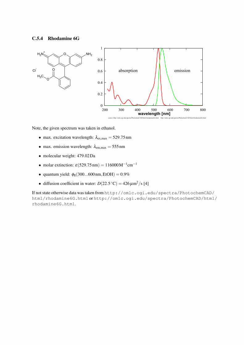
C.5.4 Rhodamine 6G
Note, the given spectrum was taken in ethanol.
• max. excitation wavelength: λex,max = 529.75nm
• max. emission wavelength: λem,max = 555nm
• molecular weight: 479.02Da
• molar extinction: ε(529.75nm) = 116000M−1cm−1
• quantum yield: φfl(300...600nm,EtOH) = 0.9%
• diffusion coefficient in water: D(22.5 ◦C) = 426 µm2/s [4]
If not state otherwise data was taken from http://omlc.ogi.edu/spectra/PhotochemCAD/html/rhodamine6G.html or http://omlc.ogi.edu/spectra/PhotochemCAD/html/rhodamine6G.html.
Appendix D
Mathematical definition of theautocorrelation function
This appendix gives a pictorial description of how autocorrelation works.
g(τ) =〈δ I(t) ·δ I(t + τ)〉t
〈I(t)〉2t=
T ·T∫
0
δ I(t) ·δ I(t + τ)dt
T∫0
I(t)dt
2 .
Figure D.1 illustrates the process of calculating the autocorrelation function g(τ). First have a lookat Fig. D.1(A). Here the signal (red curves) is a simple pulse between 0 and 1. When we shift (bluecurve) and multiply, we get a signal (green curve) which is also a pulse, but with a width, that isdecreasing with the shift τ . If we then integrate over this green signal (calculate the area below thecurve), we get the values depicted as curve in the right plot, which is already the autocorrelationfunction. It can easily be seen that the width of the triangle in g(τ) corresponds to the width ofthe pulse. Figure D.1(B) shows the same process, but for a train of pulses between 0 and 1. If theshift τ is approaching the inter pulse time ∆t, the area below the multiplied signals I(t) · I(t + τ) isincreasing again and as a result we obtain an autocorrelation curve with a series of triangles. FigureD.1(C) finally shows a more relevant example: The left graph shows a signal (red) which consistsof pulses (blue) with random length and an overlayed gaussian noise. The right graph displays theautocorrelation function of this signal on a semi-logarithmic scale. Also here we observe that thewidth τdecay of the decrease in correlation for small lags corresponds with the average length of thepulses (compare upper and lower curves).
25
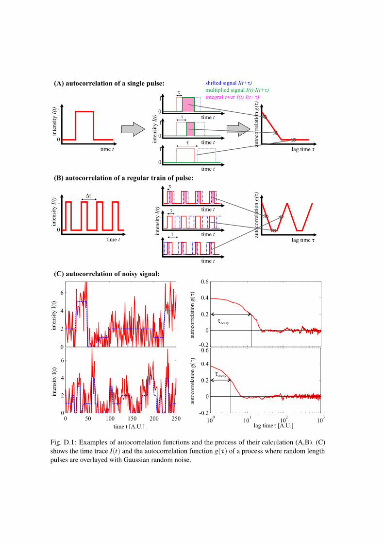
Fig. D.1: Examples of autocorrelation functions and the process of their calculation (A,B). (C)shows the time trace I(t) and the autocorrelation function g(τ) of a process where random lengthpulses are overlayed with Gaussian random noise.
Appendix E
Data Fitting
For FCS evaluations we will use a method called Least-Squares Fitting during this practicalcourse. As we have seen in section 1.3 there are a lot of known models for FCS data. So if we knewall the properties of a sample we could predict how the autocorrelation curve should look. Herewe have the opposite problem: We have a measurement of the autocorrelation curve and want toestimate the parameters that best describe our measurement (e.g. the diffusion coefficient D or theparticle number N).
First of all we have to define what we mean by "best describes the measurements": From the FCSexperiment we get a set of data pairs (τ̃i, g̃i), i = 1,2,3, ... that form the measured autocorrelationcurve, i.e. for some lag times τ̃1, τ̃2, τ̃3, ..., we get the value of the correlation curve g̃1, g̃2, g̃3, ...(see Fig. E.1(a) for an example). If we now assume that some model g(τ;N,τD) (e.g. from equation(1.3.2) with a fixed value for γ) describes the measurement, we can evaluate this model function fora given parameter set (N,τD) for every τ̃1. This gives us a set of estimates g(m)
i = g(τ̃i;N,τD) thatwe can compare to the measurements (see Fig. E.1(b) ). To determine how far the model lies awayfrom the measurement, we can simply calculate the squared distance (g̃i−g(m)
i )2 and sum over allthese values:
χ2(N,τD) =
K
∑i=1
(g̃i−g(m)i )2 =
K
∑i=1
(g̃i−g(τ̃i;N,τD))2 (E.0.1)
We use the square of the distance, so negative and positive distances do not cancel each other out.This function now only depends on the values for the two parameters N and τD and we are leftwith the problem to find the parameter combination (N̂, τ̂D) that minimizes χ2(N,τD), i.e. bestdescribes the data. To do so, we can look at the surface formed by evaluating χ2(N,τD) for differentcombinations of parameters (see Fig. E.1(c)). Then we have to find the deepest valley in this "searchlandscape". This is the same problem, as finding a protein configuration/structure with minimumenergy, in protein folding simulations/structure prediction. But in that case the parameter space ismuch larger (not only N and τD, but all the atoms positions in space).
27
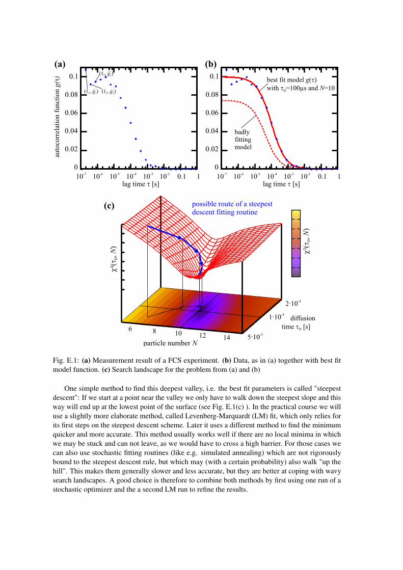
Fig. E.1: (a) Measurement result of a FCS experiment. (b) Data, as in (a) together with best fitmodel function. (c) Search landscape for the problem from (a) and (b)
One simple method to find this deepest valley, i.e. the best fit parameters is called "steepestdescent": If we start at a point near the valley we only have to walk down the steepest slope and thisway will end up at the lowest point of the surface (see Fig. E.1(c) ). In the practical course we willuse a slightly more elaborate method, called Levenberg-Marquardt (LM) fit, which only relies forits first steps on the steepest descent scheme. Later it uses a different method to find the minimumquicker and more accurate. This method usually works well if there are no local minima in whichwe may be stuck and can not leave, as we would have to cross a high barrier. For those cases wecan also use stochastic fitting routines (like e.g. simulated annealing) which are not rigorouslybound to the steepest descent rule, but which may (with a certain probability) also walk "up thehill". This makes them generally slower and less accurate, but they are better at coping with wavysearch landscapes. A good choice is therefore to combine both methods by first using one run of astochastic optimizer and the a second LM run to refine the results.
Appendix F
Anomalous Diffusion
F.1 Introduction
When looking at diffusion in cells the situation is a bit more complex than described above forthe simple case of diffusion in liquids. Cells are much more complicated objects than solutions.They are compartmentalized by membranes and the space in between is filled with different sizedorganelles, vesicles, (macro-)molecules and so forth. The cellular nucleus contains chromatinwhich fills about 10-20% of the available space, together with the protein machinery for the DNAtranscription. This already shows that diffusion may no longer be described by only small watermolecules bumping into the observed particle, but there is now a whole distribution of smaller andlarger sized particles which collide with each other (crowding). In addition the observed particle mayalso bind to certain structures in the cell (membranes, vesicles, DNA, ...), or it may be transportedactively along e.g. the cytoskeleton. Inside the nucleus the space is compartmentalized by thechromatin network which also hinders the diffusion. For this special case of hindered Brownianmotion, the diffusion may be described by a slightly modified mean squared displacement (compareequation (1.2.1) and Fig. F.1(A)):
⟨r2⟩= Γ · τα , 0 < α < 1 (F.1.1)
where α is called anomality parameter (for α = 1 (F.1.1) resembles (1.2.1)) and Γ is the propor-tionality constant. In this model the particles do not reach as far as normally diffusing particles inthe same time τ , as they may get stuck in cages or dead ends.
Figure F.1(B) once again summarizes the effects described above, which will influence yourdiffusion measurements inside living cells.
29
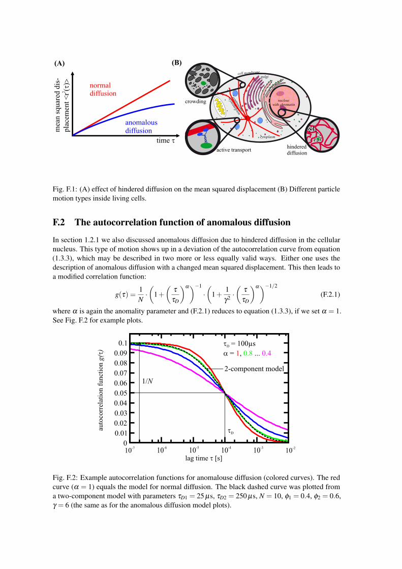
Fig. F.1: (A) effect of hindered diffusion on the mean squared displacement (B) Different particlemotion types inside living cells.
F.2 The autocorrelation function of anomalous diffusion
In section 1.2.1 we also discussed anomalous diffusion due to hindered diffusion in the cellularnucleus. This type of motion shows up in a deviation of the autocorrelation curve from equation(1.3.3), which may be described in two more or less equally valid ways. Either one uses thedescription of anomalous diffusion with a changed mean squared displacement. This then leads toa modified correlation function:
g(τ) =1N·(
1+(
τ
τD
)α)−1
·(
1+1γ2 ·(
τ
τD
)α)−1/2
(F.2.1)
where α is again the anomality parameter and (F.2.1) reduces to equation (1.3.3), if we set α = 1.See Fig. F.2 for example plots.
Fig. F.2: Example autocorrelation functions for anomalouse diffusion (colored curves). The redcurve (α = 1) equals the model for normal diffusion. The black dashed curve was plotted froma two-component model with parameters τD1 = 25 µs, τD2 = 250 µs, N = 10, φ1 = 0.4, φ2 = 0.6,γ = 6 (the same as for the anomalous diffusion model plots).
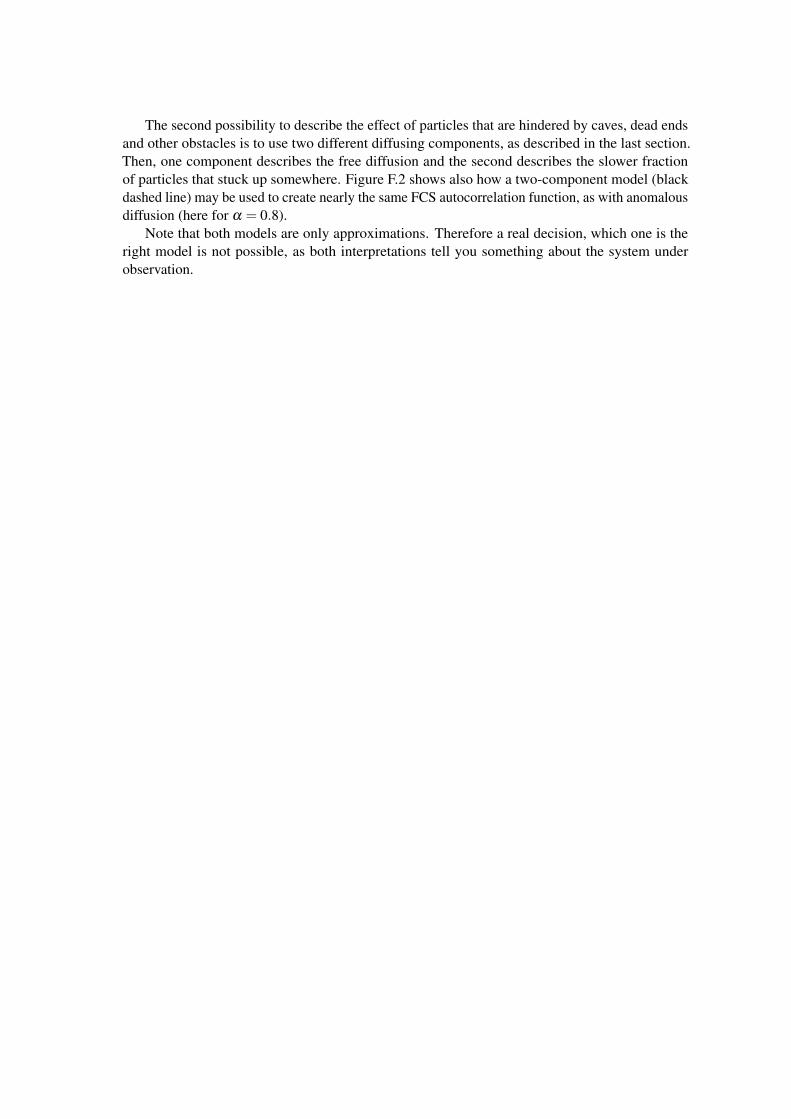
The second possibility to describe the effect of particles that are hindered by caves, dead endsand other obstacles is to use two different diffusing components, as described in the last section.Then, one component describes the free diffusion and the second describes the slower fractionof particles that stuck up somewhere. Figure F.2 shows also how a two-component model (blackdashed line) may be used to create nearly the same FCS autocorrelation function, as with anomalousdiffusion (here for α = 0.8).
Note that both models are only approximations. Therefore a real decision, which one is theright model is not possible, as both interpretations tell you something about the system underobservation.
References
[1] N. Dross. Mobilität von eGFP-Oligomeren in lebenden Zellkernen. dissertational the-sis, Universität Heidelberg, 2009. http://archiv.ub.uni-heidelberg.de/volltextserver/volltexte/2010/10470/pdf/Dross_Mobilitaet_von_eGFP_Oligomeren_in_lebenden_Zellkernen.pdf.
[2] N. Dross, C. Spriet, M. Zwerger, G. Müller, W. Waldeck, and J. Langowski. Mapping egfpoligomer mobility in living cell nuclei. PLoS ONE, 4(4):e5041, 2009. http://www.dkfz.de/Macromol/publications/files/Dross2009.pdf.
[3] G. Patterson, R. Day, and D. Piston. Fluorescent protein spectra. J Cell Sci, 114(5):837–838,2001.
[4] Z. Petrásek and P. Schwille. Precise measurement of diffusion coefficients us-ing scanning fluorescence correlation spectroscopy. Biophysical Journal, 94:1437–1448, 2008. http://www.pubmedcentral.nih.gov/picrender.fcgi?artid=2212689&blobtype=pdf.
[5] P. Reiser. Sucrose: properties and applications. Springer Netherlands, 1995.
[6] M. Wachsmuth, W. Waldeck, and J. Langowski. Anomalous diffusion of fluorescent probes in-side living cell nuclei investigated by spatially-resolved fluorescence correlation spectroscopy. J.Mol. Biol., 298:677–689, 2000. http://www.dkfz.de/Macromol/publications/files/Wachsmuth2000.pdf.
[7] R. Weast, M. Astle, and W. Beyer. CRC handbook of chemistry and physics, volume 69. CRCpress Boca Raton, FL, 1988.
32


![DOI:10.1002/cphc.200600589 ... · (FCS) andimage correlation spectroscopy.[10] Thesecond isto consider the photon-counting histogram[11,12] (PCH), as done, for example, in fluorescence](https://static.fdocuments.in/doc/165x107/5fdb3f5ac74261633f622a93/doi101002cphc200600589-fcs-andimage-correlation-spectroscopy10-thesecond.jpg)